Writing an Introduction / Personality & Risk Taking
Lab 6
PSY 395 Fall 2013
Descriptive Statistics and Histograms
• You should get in the habit of taking a peek at the data.
– Calculate relevant descriptive statistics and take a look at how a variable is distributed. Does it look normal?

You can get Descriptive statistics and a Plot with one function:
Descriptive Statistics Frequencies
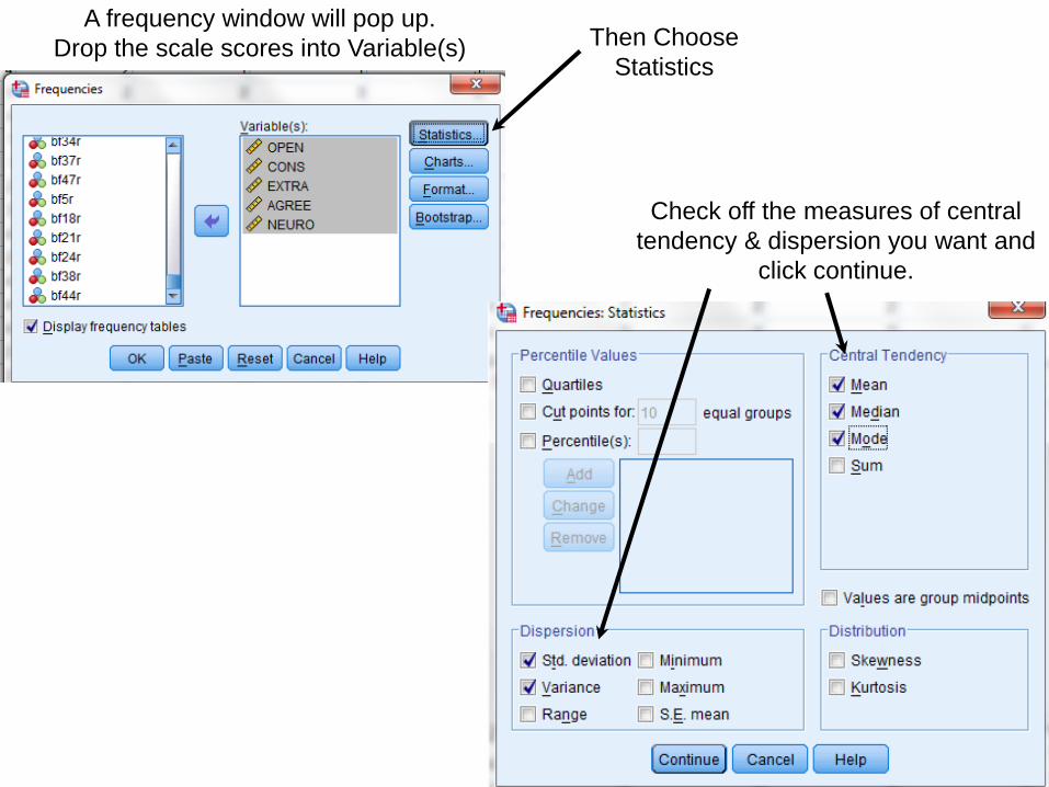
A frequency window will pop up.
Drop the scale scores into Variable(s) Then Choose
Statistics
Check off the measures of central
tendency & dispersion you want and
click continue.

Then choose Charts
Select
Histograms &
Check mark
“With normal
curve”

You will get the descriptive stats in
Output.
Ask yourself: Is this the mean and
standard deviation I would expect?
You will get a
histogram and
normal plot. Do the
data look normally
distributed?

• We often want to know if two variables go up and down together or if one goes up while the other goes down.
– Is alcohol consumption (Y) negatively related to heart disease (X)?
– Does the accuracy of performance (Y) decrease as speed of response (X) increases?
– Are people who are high in extraversion also high in openness?
Correlation
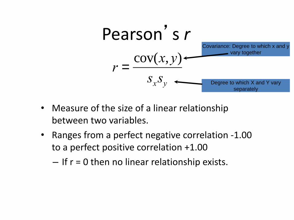
Pearson’s r
• Measure of the size of a linear relationship between two variables.
• Ranges from a perfect negative correlation -1.00 to a perfect positive correlation +1.00
– If r = 0 then no linear relationship exists.
r =cov(x, y)
sxsy
Covariance: Degree to which x and y
vary together
Degree to which X and Y vary
separately
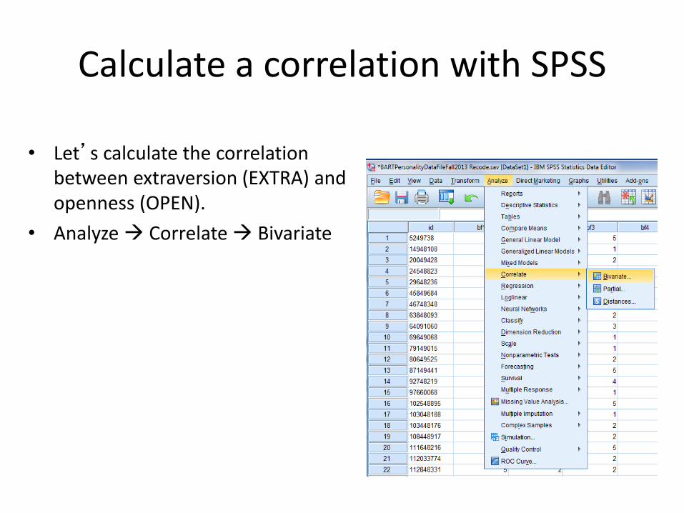
Calculate a correlation with SPSS
• Let’s calculate the correlation between extraversion (EXTRA) and openness (OPEN).
• Analyze Correlate Bivariate

Drop EXTRA and OPEN into the Variables window.
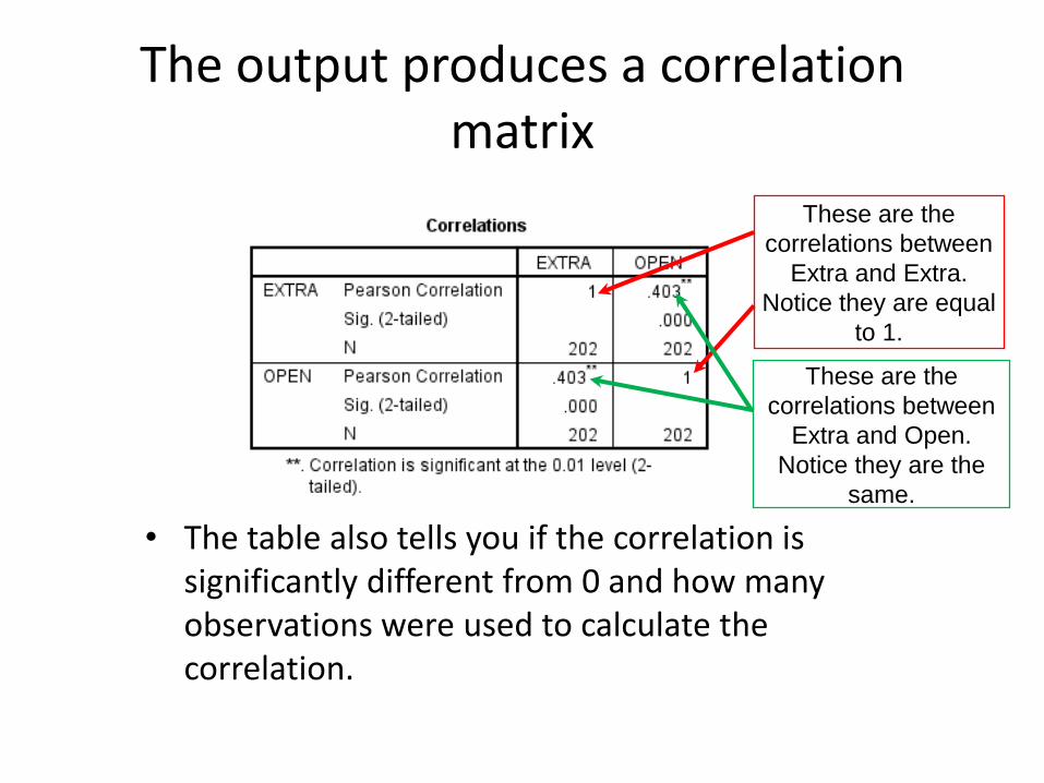
The output produces a correlation matrix
• The table also tells you if the correlation is significantly different from 0 and how many observations were used to calculate the correlation.
These are the
correlations between
Extra and Extra.
Notice they are equal
to 1.
These are the
correlations between
Extra and Open.
Notice they are the
same.

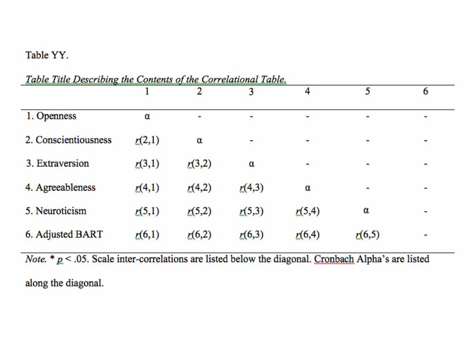
Tables
Note only horizontal lines are
used to organize the table.
Basically only a bottom and top
line around the column labels.
And a line at the bottom.
Make it easy for the reader to
compare the data you want
them to compare.

• Recall, reliability is a measure of how consistent a test score is. Different types of consistency:
•test-retest
•internal consistency (alpha)
•interobserver/interrater
Reliability

• Quantifies how much consistency there is between the items in a scale
–How well do the items “hang together”?
• If different items in a scale are consistently measuring the construct of interest, we should find associations between all of the items…
Internal Consistency

• The first step is to look at the Inter-item correlation Matrix
• For example, we can examine the associations between each of the items that comprise the Extraversion scale.
• Under Analyze
–Correlate Bivariate
–Select all items in the Time 1 Extra scale (11R, 23R, 2, 16, 17, 32, 41, 43, 45, 49)
–Click OK
Internal Consistency
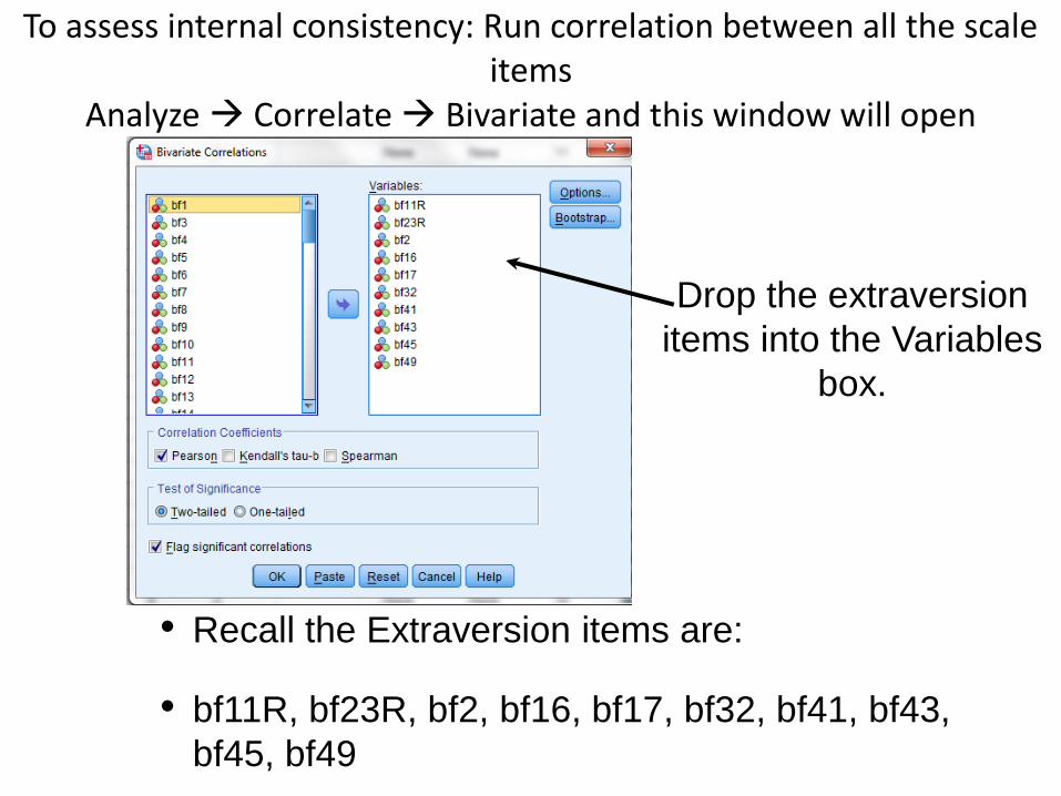
Drop the extraversion
items into the Variables
box.
• Recall the Extraversion items are:
• bf11R, bf23R, bf2, bf16, bf17, bf32, bf41, bf43,
bf45, bf49
To assess internal consistency: Run correlation between all the scale items
Analyze Correlate Bivariate and this window will open
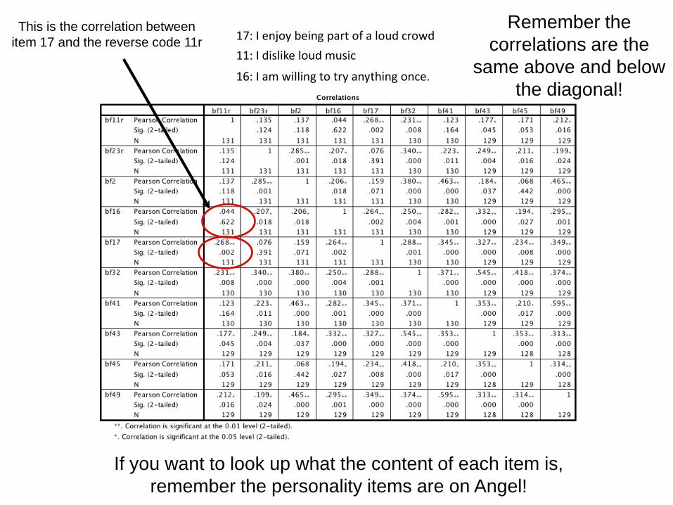
This is the correlation between
item 17 and the reverse code 11r 17: I enjoy being part of a loud crowd
11: I dislike loud music
If you want to look up what the content of each item is,
remember the personality items are on Angel!
16: I am willing to try anything once.
Remember the
correlations are the
same above and below
the diagonal!
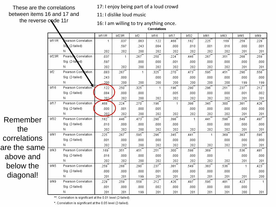
These are the correlations
between items 16 and 17 and
the reverse code 11r
17: I enjoy being part of a loud crowd
11: I dislike loud music
16: I am willing to try anything once.
Remember
the
correlations
are the same
above and
below the
diagonal!
• Examine the matrix carefully. What is the range of correlations? Are there any particularly low values? Any particularly high values?
• Download the excel sheet with the Personality Items and take a look at the individual items. Do the high inter-item correlations make sense? How about the low ones?

Calculating Alpha by Hand
a =kri, j
1+ k -1( )ri, j
k: number of items average inter-item
correlation
ri , j :

Calculate Alpha
• Say the average inter-item correlation for our extraversion scale was = .27. What is Alpha for k = 10?
• Now imagine we had the same inter-item correlation but now calculate Alpha for
– k = 20, k = 40, k = 80, k = 160 ri , j
ri , j
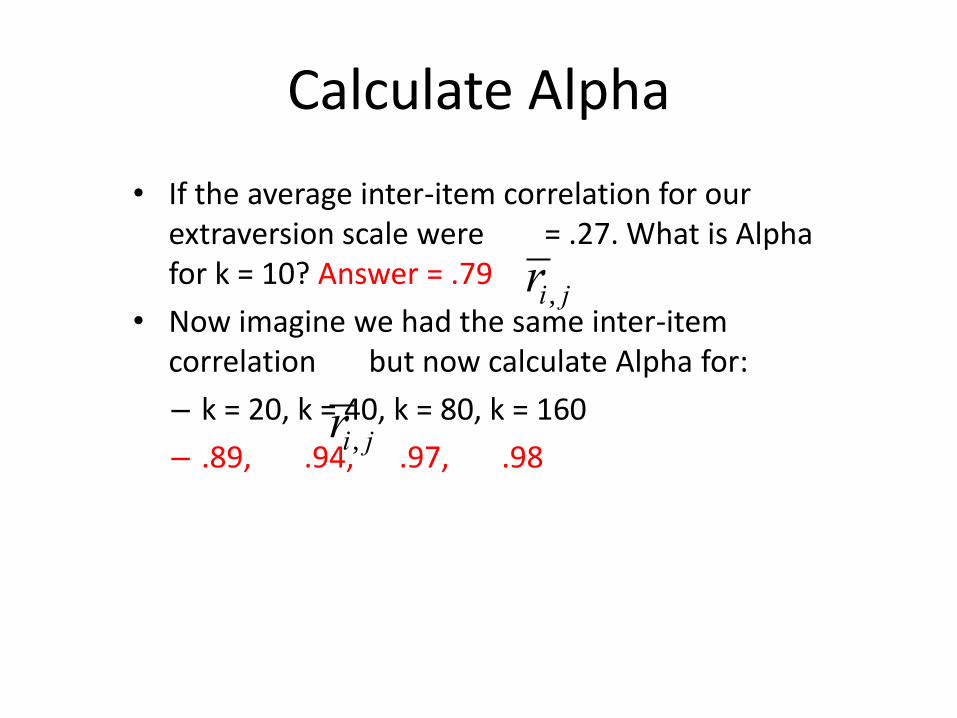
Calculate Alpha
• If the average inter-item correlation for our extraversion scale were = .27. What is Alpha for k = 10? Answer = .79
• Now imagine we had the same inter-item correlation but now calculate Alpha for:
– k = 20, k = 40, k = 80, k = 160
– .89, .94, .97, .98 ri , j
ri , j
Why does Alpha approach 1 as you add more unique items?
• Remember our measures of reliability are telling us how much measurement error there is. As we add more unique items then we reduce the impact of measurement error.
• But, no one wants to take a 1000 item inventory!
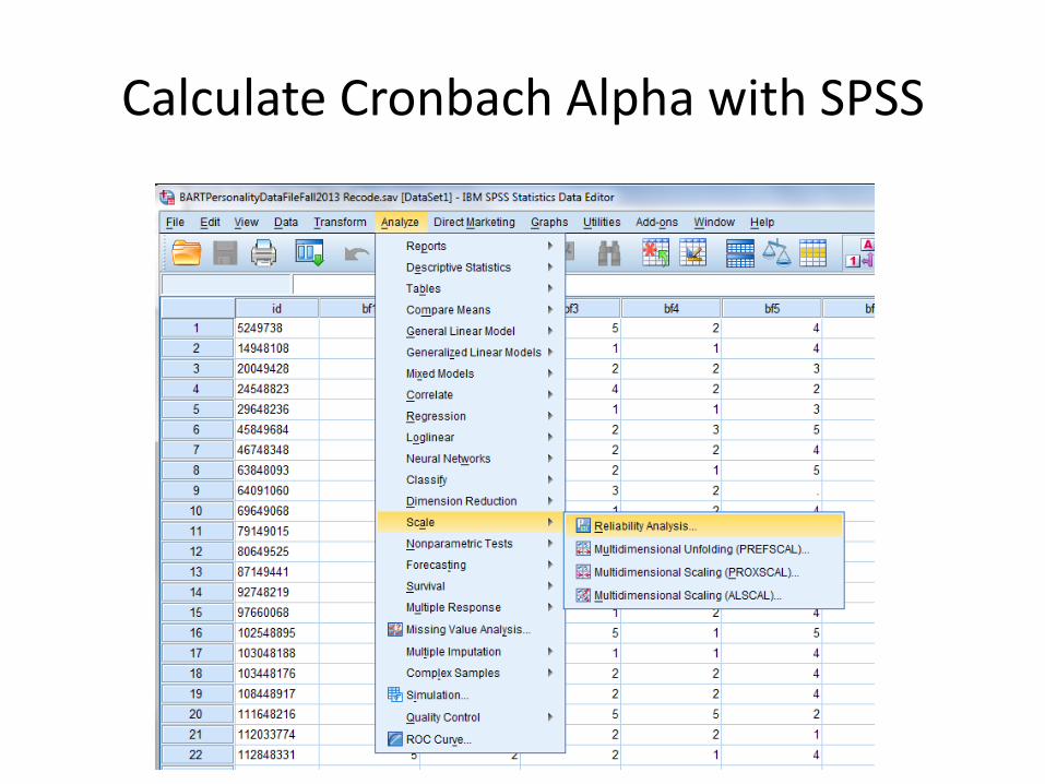
Calculate Cronbach Alpha with SPSS

Drop the items for the scale of
interest (e.g., extraversion) into
the item box.
Choose Alpha
And type in a
Scale Label
Want to know a trick?
You can get a lot of good stuff out of the statistics option. Click it
and take a look.
You can get:
inter-item correlation matrix
mean inter-item correlation
means and sd for each item
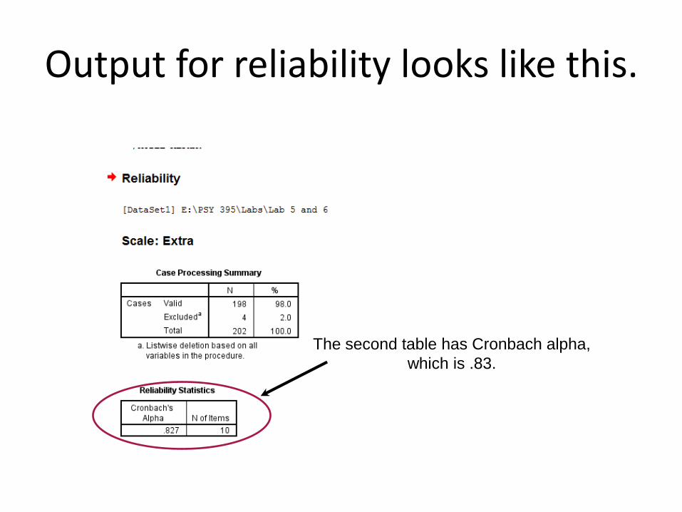
Output for reliability looks like this.
The second table has Cronbach alpha,
which is .83.

• Examine the inter-item correlation matrices for the other Time 1 Big Five scales. – Openness (bf9, bf35, bf39, bf50, bf5R, bf18R, bf21R, bf24R, bf38R, bf44R)
– Conscientiousness (bf19, bf25, bf40, bf10R, bf14R, bf20R, bf27R, bf29R, bf36R, bf42R)
– Extraversion (just performed in the slides above)
– Agreeableness (bf6, bf8, bf12, bf28, bf31, bf46, bf3R, bf4R, bf13R, bf15R)
– Neuroticism (bf7, bf22, bf30, bf33, bf48, bf1R, bf26R, bf34R, bf37R, bf47R)
Internal Consistency
You will need this for your table in your Lab Report 3!

Construct Validity
• Does a particular measurement truly measure the construct?
– THINK: OPERATIONAL DEFINITION.
• The extent to which the variables accurately reflect or measure the behavior of interest.
Assessing Construct Validity
• Correlate the measure with measurements of similar but distinct traits (divergent validity).
– Correlate extraversion with agreeableness, extraversion with openness, etc., they should not be strongly correlated.
• Could also compare the measurement with other measures with the same trait.
– Correlation extraversion from the Big 5 inventory with extraversion Eysenck’s personality scale.

In SPSS correlate the 5 scale scores

Drop the scale scores
into the variables box.
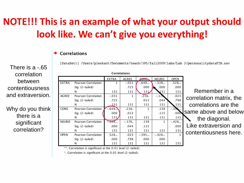
There is a -.65
correlation
between
contentiousness
and extraversion.
Why do you think
there is a
significant
correlation?
Remember in a
correlation matrix, the
correlations are the
same above and below
the diagonal.
Like extraversion and
contentiousness here.
NOTE!!! This is an example of what your output should look like. We can’t give you everything!

Criterion Validity
• Can a measure accurately forecast some future behavior, or
• Is a measure related to some other measure of behavior?
• In our study, our criterion is risky decision making in the BART.

For our criterion, we will use the BART
• Recall, we are going to use the average number of pumps taken on non-exploding balloons (adjusted BART score) as a measure of risk taking.
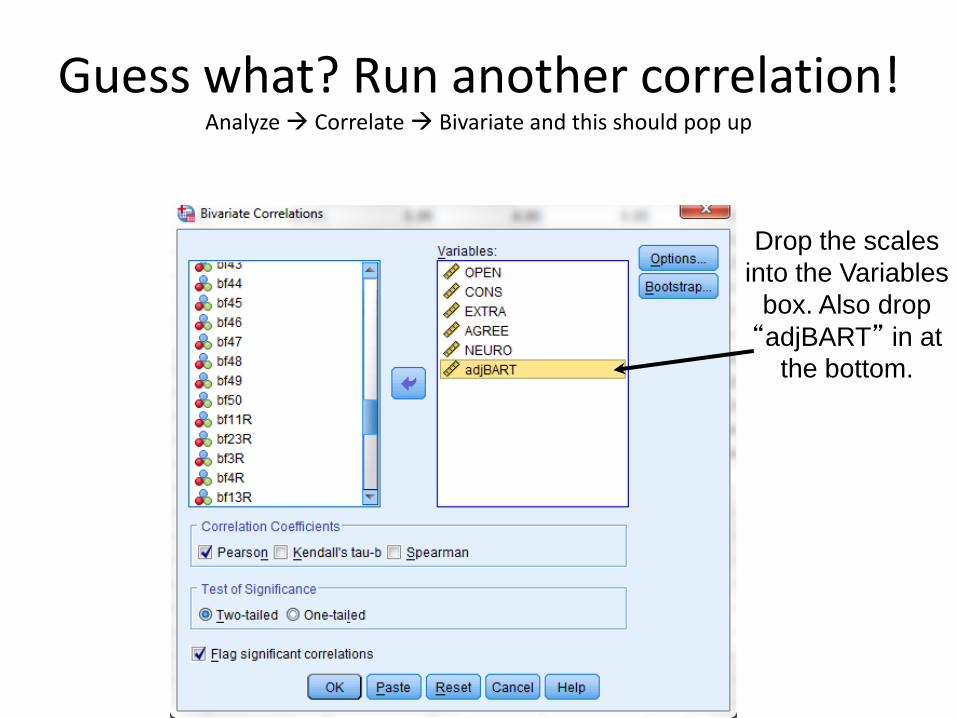
Guess what? Run another correlation! Analyze Correlate Bivariate and this should pop up
Drop the scales
into the Variables
box. Also drop
“adjBART” in at
the bottom.
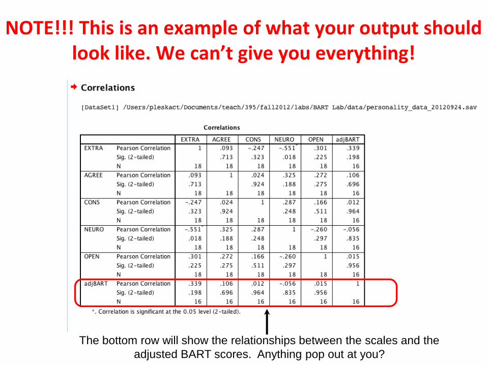
The bottom row will show the relationships between the scales and the
adjusted BART scores. Anything pop out at you?
NOTE!!! This is an example of what your output should look like. We can’t give you everything!

For Lab Report 3
• Do a lit search for three peer-reviewed articles to motivate your hypothesis about an association between a personality factor and risky decision making.

For your lab report
• Report in a correlation table the inter-correlations between the personality scales and the adjusted BART scores from the BART.
– List the correlations between the diagonal.
– List the reliability (Cronbach Alphas) of the scales along the diagonal.

Here is what the table should look like.

References and in text citations
• When you write a paper you need to cite the sources you are drawing your ideas from, using or adapting methods from, using or adapting analyses from, etc.
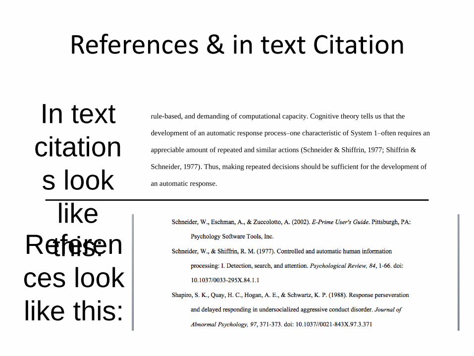
References & in text Citation
MAKING ASSESSMENTS WHILE TAKING REPEATED RISKS 3
Making Assessments While Taking Repeated Risks:
A Pattern of Multiple Response Pathways
Risks like texting while driving, eating unhealthy food for a quick lunch, or smoking a
cigarette, are typically not one-shot choices. Rather, these are choices that are made repeatedly
over the course of a day, a week, a month, and so on. Repeated decisions put different demands
on a cognitive system than one-shot choices. They, for example, allow for and even may require
learning (Busemeyer & Stout, 2002; Denrell, 2007; Pleskac, 2008; Wallsten, Pleskac, & Lejuez,
2005) as well as search and exploration (Daw, O'Doherty, Dayan, Seymour, & Dolan, 2006).
They also put different demands on attention and memory (Barron & Erev, 2003) and may even
change the decision process itself (Jessup, Bishara, & Busemeyer, 2008). In this paper, we
examine how multiple response pathways develop while people make repeated decisions.
Judgments and decisions under uncertainty are often described as being made with one of
two information-processing systems: System 1 or System 2 (Evans, 2008; Kahneman, 2003;
Mukherjee, 2010; Reyna, 2004; Sloman, 1996; Stanovich & West, 2000) (cf. Gigerenzer &
Regier, 1996; Keren & Schul, 2009; Kruglanski & Gigerenzer, 2011). System 1 makes
judgments that are fast, automatic, effortless, associative in nature, and undemanding on
computational capacity. System 2, in comparison, makes judgments that are slower, controlled,
rule-based, and demanding of computational capacity. Cognitive theory tells us that the
development of an automatic response process–one characteristic of System 1–often requires an
appreciable amount of repeated and similar actions (Schneider & Shiffrin, 1977; Shiffrin &
Schneider, 1977). Thus, making repeated decisions should be sufficient for the development of
an automatic response.
In text
citation
s look
like
this: Referen
ces look
like this:

References
• https://owl.english.purdue.edu/owl/resource/560/05/
• http://libguides.lib.msu.edu/citeinfo
• The format changes depending if you have: – A journal article with one author
– A journal article with more than one author
– A magazine
– A book
– Electronic sources
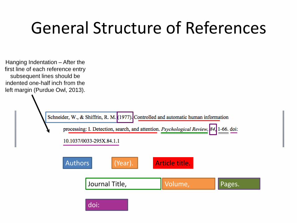
General Structure of References
Authors (Year). Article title.
Journal Title, Volume, Pages.
doi:
Hanging Indentation – After the
first line of each reference entry
subsequent lines should be
indented one-half inch from the
left margin (Purdue Owl, 2013).

DOI’s • Digital Object Identifiers: unique alphanumeric identifiers that lead
users to digital source material
– They are like a paper’s email address

Here is what a reference section looks like in an unpublished report
Lab Report 3
• Due by the start of Lab during the week of October 28th.
• READ ALL DIRECTIONS!
• Ask me – your amazing and friendly TA (Weaver, 2013) – if you have any questions.


