
VOL. 13, NO. 20, OCTOBER 2018 ISSN 1819-6608
ARPN Journal of Engineering and Applied Sciences ©2006-2018 Asian Research Publishing Network (ARPN). All rights reserved.
www.arpnjournals.com
8172
X-RAY DIFFRACTION LINE PROFILEANALYSIS OF CERIUM OXIDE
NANO PARTICLE BY USING DOUBLE VOIGT FUNCTION METHOD
Mustafa Mohammed Abdullah and Khalid Hellal Harbbi
Department of Physics, College of Education (Ibn Al-Haitham), University of Baghdad, Iraq
E-Mail: [email protected]
ABSTRACT
In this research, the double Voigt method was used to analyze the X-ray lines and then to use the Williamson-Hall
method for estimate the particle size and lattice strain of cerium oxide nanoparticle. The value of the crystallite size was
equal to (12.4964nm) and the emotion was equal to (0.006819). In addition, other methods have been used in addition to
the double Voigt method for the calculation of crystallite size and lattice strain. These methods are (Sherrer method, size-
strain plot (SSP) method and Halder-Wagner method) and their results are as follows Sherrer crystallite size (7.6386 nm)
and lattice strain (0.01039), SSP method crystallite size (59.8956 nm) and lattice strain (0.00157), and Halder-Wagner
method crystallite size (9.2287nm) and lattice strain (0.00267). The double Voigt method combined with Williamson Hall
method gave very accurate results in calculating both crystallite size and lattice strain by taking a full diffraction curve
during calculations.
Keywords: crystallite size, lattice strain, doubles Voigt method, Sherrer method, size-Strain plot method, Halder-Wagner method.
INTRODUCTION X-ray diffraction is a gadget for the investigation
of the particular magnificent structure associated with the
issue. This technique considered the precise origins in von
Laue's finding in 1912, that will deposit diffract x-rays.
The exclusive way with the diffraction exposing the
unique arrangement associated with the specific crystal.
At first, x-ray diffraction was utilized only for the
dedication of crystal structure. Other uses had been
developed; today the particular method is applied. Not
unique to the structure dedication, but two such diverse
problems as chemical evaluation and stress measurement
to the study of stage equilibria and the dimension of
particle size. In order to the determination of the particular
inclination of one amazingly or the ensemble associated
with directions in a polycrystalline aggregate [1]. The
investigation of the peaks developed by x-ray diffraction
their shapes is the well-developed and valuable technique
for the study associated with the magnificent structure of
crystalline materials. This method is identified as
Diffraction Peak profile Analysis (DPPA). It is usually a
statistical method since uses information via the single
diffraction style, which comprehends details through
many grains. From this particular pattern, a DPPA
technique quantifies the magnificent structure associated
with a sample [2]. A pure crystal would extend almost
everywhere to infinity; however, definitely, no crystals
are perfect because of their finite size. This change from
perfect crystalline the reason for broadening of the
particular diffraction peaks of components. You can find
two main characteristics extracted from peak width
analysis they are crystallite volume and lattice strain.
Crystallite dimension calculation is linked to the size of
the specification coherently diffracting domain. Since
well as the crystallite size of the exacting grains is not
genuinely usually the particular same as the specific
particle bulk due to the presence of polycrystalline
aggregates. Lattice strain is usually a measure of the
selective distribution of lattice constants as a result of
crystal imperfections, this rather as lattice dislocation [3].
One of diffraction peak profile analysis is Scherrer’s
formula it is the particular most of the known technique
for extracting size facts from powder designs (namely,
from Bragg peaks’ width). It is the particular
straightforward method, but accurate only to the order of
magnitude. Nevertheless, provided that Scherrer’s work
selection, profile analysis distributes made huge progress
[4]. In a variety of ways, Bragg peak will be influenced by
crystallite dimension and lattice stress. Usually raise the
peak width plus strength shifting the 2θ top position accordingly. The particular crystallite bulk changes
because 1/cos θ and strain vary as tan θ from the peak size. The scale and stress results on the peak increasing
are usually known from the difference of 2θ. W-H
analysis is emphatically an integral breadth method. Size-
induced and strain-induced increasing are intricate simply
by considering the peak size as a function associated with
2θ [5]. “Double Voigt” is a diffraction peak profile
analysis method, used the Voigt function that derived
equations by Langford to convolution the curves and
showed that the Cauchy broadened and Gaussian
broadened can be easily determined from the ratio of
FWHM of the broadened profile to the integral breadth
[6].
Theory
Double Voigt method The double Voigt method use a Voigt function
for fitting line profile, this function can find by
convolution of the Gaussian (G) and Lorentzian (L)
functions [6]. Additional to the line broadening there is a
source broadening called “instrument broadening” in this
broadening the correction can made by suppose that
experimental profile h(x) is involution of the sample
profile f(x) and instrumental assistance g(x).
h(x) = f(x) * g(x) (1)
VOL. 13, NO. 20, OCTOBER 2018 ISSN 1819-6608
ARPN Journal of Engineering and Applied Sciences ©2006-2018 Asian Research Publishing Network (ARPN). All rights reserved.
www.arpnjournals.com
8173
By assuming the (f,g,h) is a Voigt function the
information of the f(x) can find, from equation. (2.3) we
find:
βfL = βhL – βgL (2 a)
And
β2fG = β2
hG - β2gG (2 b)
βiG and βiL are the Gaussian (G) and the
Lorentzian (L) component of the profile i(x) of the
integral breadth [7].
The integral breadth β = A / Io (3)
Where A is the area of the peak and Io is the
height of the line profile, the two equations above the line
broadening is assigned to the action of the domain size.
β = K λ /<L>cosθ (4)
This equation showed that the finite size of the
crystal made the broadening of very small crystals, the β was the width must be in radian and the k is constant 0.89
and λ is the wave length which is 0.15406 nm, θ is the Bragg angle and <L> is the average column length it is
similar to the length of the circle but it was parallel to the
diffracted plane in this status therefor there is a relation of
the volume weighted crystal diameter and the volume
weighted column length which is
<D> = 4/3 <L> (5)
The strain can be estimated via equation:
β = η tanθ (6)
Where η is the strain and the 2θ dependence in this relation was deferent from that in the equation. (2.6)
it was the reason that allowed to separate the action of the
strain and the size on peak broadening.
β cos θ = (K λ/<L> ) + η sin θ (7)
This equation is similar to the form y=b +mx, the
η can obtain from the slope between sin θ and β cos θ and <L> can obtain from the intercept.
In the single line profile process the crystallite
size will give the Lorentz component and the strain can
appears the Gaussian component.
The equation. (4) can use to produce the apparent
domain size by replacing β by βL and use the equation. (6)
to gives the strain by replacing β by βG, βL for the
Gaussian and Lorentzian component of the integral
breadth.
To stop the “hook” effect accomplish the
conditions must be taken [8][9]:
βCS= (π/2)1/2 βGS (8)
2w/β ratio for both h and g profiles where 2w is the FWHM and β is the breadth, for Lorentz reflections the ratio [10] [11]:
2w/β = 2/π = 0.63662 for Lorentz profile (9)
And for Gaussian reflections the ratio can be:
2w/β = 2*(ln (2))1/2/ π1/2 = 0.93949 for Gaussian profile (10)
The crystallite size and the strain in this method
is calculated using the plot of W-h , additional also the
size and the strain is calculated but with separation which
is an analytical method that use equations and arithmetic
mean.
Sherrer method
The broadening of line diffraction profile can be
happen from the finite crystallite size, strain and the
defects of deflection from ideal crystallinity, the
crystallite size can be measure by the equation that
produce by Debye Sherrer in 1918:
Dv = (K λ /FWHM) cos θ (11)
Where K is a shape factor (0.89) and θ is the Bragg angle and λ is the wavelength (0.15406 nm) and Dv is the
volume weighted quantity and FWHM full width at half
maximum of the intensity of the peak
The strain ε can obtain from line broadening which measure by the equation [12]:
ε= β cot θ /4 = β/4 tan θ (12)
Where β is the integral breadth and ε is the strain
Williamson-Hall method
The crystallite size and lattice these two factors
additional to the instrumental broadening are responsible
for the total line broadening and the strain can estimate by
the equation. (2.14), the total broadening can obtain by
take the summation of these two factors in the material,
by assuming that the strain is in the uniform state in the
material so that by using the W-H equation we can
estimate the crystallite size and the strain [13]:
βh k l = βs + βD (13)
βh k l = (K λ /D cos θ) +4 ε tan θ (14)
And the equation. (2.16) is multiply by cos θ therefor the equation can be:
βh k l cos θ = (K λ /D) + 4 ε sin θ (15)
Where K is the shape factor (0.89) and βh k l is
integral breadth and λ is the wavelength (0.15406 nm) and D is the crystallite size in nm and ε is the lattice strain. The size can obtain by the intercept and the strain can
obtain by the slope [14].

VOL. 13, NO. 20, OCTOBER 2018 ISSN 1819-6608
ARPN Journal of Engineering and Applied Sciences ©2006-2018 Asian Research Publishing Network (ARPN). All rights reserved.
www.arpnjournals.com
8174
Size-strain plot method (SSP) The estimation of the size and the strain can be
done by observing the average “size-strain plot” (SSP),
the feature of this method that at high reflection angles
lower value was given, and less precision can be obtain,
the crystallite size was considering to be qualified by
Lorentz function and the strain was considering to be
qualified by Gaussian function:
(d βh k l cos θ)2 = (K/D) (d
2 βh k l cos θ) + (ε/2)2
(16)
K was the shape factor in the study the value was
0.89 and the plot was between (d βh k l cos θ)2and (d
2 βh k l
cos θ) for all peaks, and d was the spacing distance that can calculate from the Bragg law, the crystallite size D
could be estimated from the slope of the data that fitted,
and the root mean square (RMS) strain could be obtained
from the Y-intercept from the plot [15].
Halder-Wagner method
In this method the average crystallite size was
estimated and the Lorentz function and Gaussian function
could be used for qualified the integral breadth, the size
and the strain could be estimated by the equation:
(β cos θ/ sin θ)2 = (K λ/D) (β / tan θ * sin θ) + 16 ε2
(17)
Where β is the integral breadth and K is the Sherrer constant (0.89) and λ is the wavelength (0.15406 nm) and D is the crystallite size in nm and ε is the weighted average strain.
By the plotting between (β cos θ/ sin θ)2 against
(β / tan θ * sin θ) the slope could give the crystallite size
and the Y- intercept gives the strain [16].
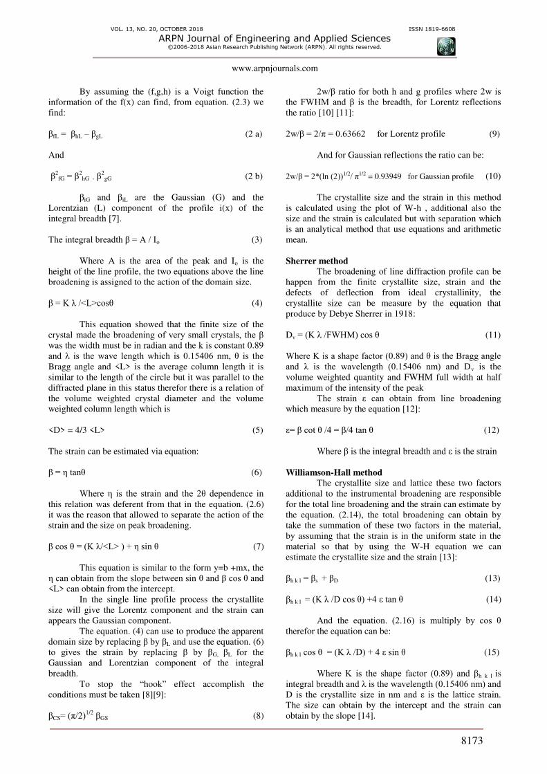
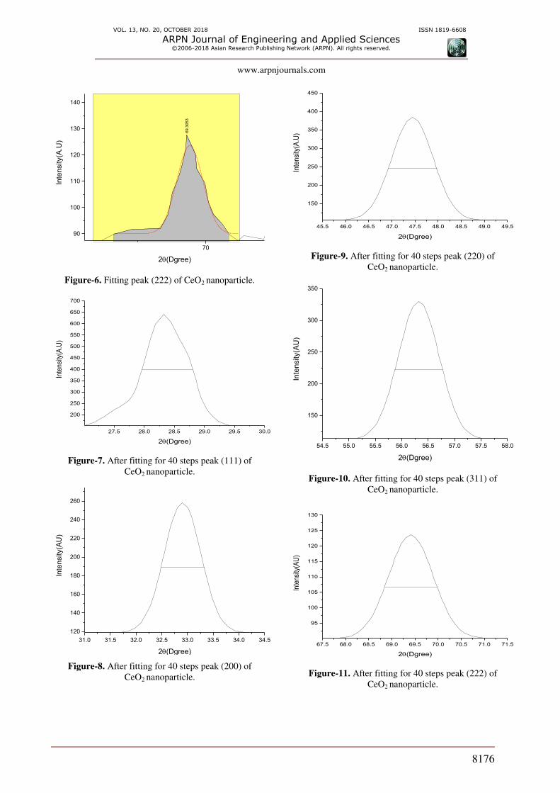
RESULTS AND DISCUSSIONS
Double Voigt method
The Voigt function was used to analysis the x-ray
diffraction line profile of the cerium oxide nanoparticle, at
first the values of the intensity and 2θ of CeO2
nanoparticle were calculated by using Get Data Graph
Digitizer program after getting the values therefor used
this values to plot the pattern of cerium oxide nanoparticle
by using Origin Pro Lab program, after that each peak in
the pattern was fitting to get the pure line of the peaks,
after fitting the peaks, 40 steps on the fitting line of each
peak was made additional to the high intensity step for
each peak to get most pure and accurate line of each peak
in the pattern, area under the curve was estimated after
subtracting intensity to get rid of background values for
each peak, after that FWHM was estimated and the
equation.(3) was used to calculate the integral breadth for
each peak.
20 30 40 50 60 70 80
0
100
200
300
400
500
600
700
inte
nsity
(AU)
2(dgree)
28.2
427
32.8
198
47.3
028
56.1
953
69.3
053
(111)
(200)
(220)
(311)
(222)
Figure-1. XRD pattern CeO2 nanoparticle by origin pro lab program.

VOL. 13, NO. 20, OCTOBER 2018 ISSN 1819-6608
ARPN Journal of Engineering and Applied Sciences ©2006-2018 Asian Research Publishing Network (ARPN). All rights reserved.
www.arpnjournals.com
8175
27.0 27.5 28.0 28.5 29.0 29.5
150
200
250
300
350
400
450
500
550
600
650
inte
nsi
ty (
AU
)
2(dgree)
28
.24
27
28
.32
332
8.3
233
Figure-2. Fitting peak (111) of CeO2 nanoparticle.
35
100
120
140
160
180
200
220
240
260
inte
nsity
(A.U
)
2(dgree)
32.8
198
Figure-3. Fitting peak (200) of CeO2 nanoparticle.
40 45 50
200
400
Intin
sity(A
.U)
2(Dgree)
47.3
028
Figure-4. Fitting peak (220) of CeO2 nanoparticle.
55 60
200
Inte
nsity
(A.U
)
2(Dgree)
56.1
953
Figure-5. Fitting peak (311) of CeO2 nanoparticle.
VOL. 13, NO. 20, OCTOBER 2018 ISSN 1819-6608
ARPN Journal of Engineering and Applied Sciences ©2006-2018 Asian Research Publishing Network (ARPN). All rights reserved.
www.arpnjournals.com
8176
70
90
100
110
120
130
140
Inte
nsity(A
.U)
2(Dgree)
69.3
053
Figure-6. Fitting peak (222) of CeO2 nanoparticle.
27.5 28.0 28.5 29.0 29.5 30.0
200
250
300
350
400
450
500
550
600
650
700
Inte
nsi
ty(A
.U)
2(Dgree)
Figure-7. After fitting for 40 steps peak (111) of
CeO2 nanoparticle.
31.0 31.5 32.0 32.5 33.0 33.5 34.0 34.5
120
140
160
180
200
220
240
260
Inte
nsity(A
U)
2(Dgree)
Figure-8. After fitting for 40 steps peak (200) of
CeO2 nanoparticle.
45.5 46.0 46.5 47.0 47.5 48.0 48.5 49.0 49.5
150
200
250
300
350
400
450
Inte
nsi
ty(A
.U)
2(Dgree)
Figure-9. After fitting for 40 steps peak (220) of
CeO2 nanoparticle.
54.5 55.0 55.5 56.0 56.5 57.0 57.5 58.0
150
200
250
300
350
Inte
nsity(A
U)
2(Dgree)
Figure-10. After fitting for 40 steps peak (311) of
CeO2 nanoparticle.
67.5 68.0 68.5 69.0 69.5 70.0 70.5 71.0 71.5
95
100
105
110
115
120
125
130
Inte
nsity
(AU
)
2(Dgree)
Figure-11. After fitting for 40 steps peak (222) of
CeO2 nanoparticle.

VOL. 13, NO. 20, OCTOBER 2018 ISSN 1819-6608
ARPN Journal of Engineering and Applied Sciences ©2006-2018 Asian Research Publishing Network (ARPN). All rights reserved.
www.arpnjournals.com
8177
Table-1. Results of CeO2 nanoparticle for peak (111).
2θ intensity intensity-
Background Area=(y1+y2)/2*(x2-x1)
27.01076 154.41055 0 0.3623782215
27.11041 161.68357 7.27302 0.8818764697
27.18728 170.08215 15.6716 1.4007745476
27.25562 179.73323 25.32268 2.2245809734
27.32679 191.60244 37.19189 2.1415301937
27.37804 200.79057 46.38002 3.255383574
27.44068 211.96998 57.55943 4.3175742013
27.50901 223.22531 68.81476 5.2698728707
27.58019 233.66752 79.25697 6.5408648408
27.65706 245.33349 90.92294 7.6411101192
27.73394 262.26779 107.85724 5.2604852325
27.77949 277.52961 123.11906 4.8601966868
27.8165 293.93384 139.52329 5.0883495217
27.85067 312.71281 158.30226 6.3111406128
27.88768 337.15885 182.7483 6.0978433284
27.919 361.05199 206.64144 12.4534507675
27.9731 408.15546 253.74491 16.8847731291
28.03289 465.46822 311.05767 24.5420023178
28.10406 533.02556 378.61501 33.9168032968
28.18663 597.32402 442.91347 63.5386838862
28.3233 641.3088 486.89825 58.9224913902
28.44857 608.24019 453.82964 51.3804301049
28.571 539.9247 385.51415 41.6200955076
28.68773 481.99664 327.58609 18.5464583039
28.74752 447.21109 292.80054 11.0590565528
28.78738 416.50497 262.09442 7.77001437
28.8187 388.48563 234.07508 5.0862972146
28.84148 366.89361 212.48306 4.0450353505
28.86141 347.85176 193.44121 3.6695914197
28.88134 329.21735 174.8068 3.7500533482
28.90411 308.9892 154.57865 3.3090898871
28.92689 290.35779 135.94724 3.242974476
28.95251 271.62291 117.21236 3.082005208
28.98099 253.63114 99.22059 3.3139525659
29.018 234.27413 79.86358 2.8500888528
29.05786 217.55193 63.14138 2.8025675562
29.10911 200.63766 46.22711 2.2200809202
29.16605 186.1631 31.75255 1.7277793973
29.23438 173.22962 18.81907 1.05707117
29.31126 163.09073 8.68018 0.4708190782
29.41945 154.43393 0.02338
Σ Area = 442.9156274657
Io/2 Area under the
curve FWHM B=Area/Io FWHM / B
442.9156274657 0.8477593557 0.9096677334 0.9319439666 2θ-1 2θ-2 Intensity
27.9601309353 28.807890291 397.8468697419

VOL. 13, NO. 20, OCTOBER 2018 ISSN 1819-6608
ARPN Journal of Engineering and Applied Sciences ©2006-2018 Asian Research Publishing Network (ARPN). All rights reserved.
www.arpnjournals.com
8178
Table-2. Results of CeO2 nanoparticle for peak (200).
2θ intensity intensity-
Background Area=(y1+y2)/2*(x2-x1)
31.69131 119.00487 0.01888 0.106341741
31.84751 120.32872 1.34273 0.3794994434
31.97838 123.4429 4.45691 0.8824039601
32.09659 129.45851 10.47252 1.0526282981
32.17258 136.21786 17.23187 1.1014687656
32.22746 141.89511 22.90912 1.2093976782
32.2739 148.16118 29.17519 1.3709795337
32.31611 154.77074 35.78475 1.48684025
32.35411 161.45599 42.47 1.5439557887
32.38788 167.95548 48.96949 1.5368922495
32.41743 174.03628 55.05029 1.983597069
32.45121 181.3778 62.39181 2.5347072362
32.4892 190.03494 71.04895 2.2019308088
32.51875 196.96789 77.9819 2.7688907774
32.55252 204.98933 86.00334 4.2482775618
32.59896 215.94034 96.95435 4.2954581558
32.64118 225.51142 106.52543 4.683819987
32.68339 234.38996 115.40397 5.5588538358
32.72983 242.98141 123.99542 8.6978855967
32.79738 252.51494 133.52895 14.4076300407
32.90292 258.48395 139.49796 13.8526988766
33.00424 252.93254 133.94655 8.7323752637
33.07178 243.62325 124.63726 5.5914126876
33.11822 235.15031 116.16432 4.7186902237
33.16044 226.35034 107.36435 4.3309002775
33.20265 216.82895 97.84296 4.6544698225
33.25331 204.89628 85.91029 2.434903452
33.28286 197.87458 78.88859 2.2292434564
33.31242 190.92578 71.93979 2.5678825735
33.35041 182.23349 63.2475 2.24608633
33.38841 173.95356 54.96757 1.534515543
33.41796 167.87734 48.89135 1.3603766543
33.44751 162.16751 43.18152 1.3562974183
33.48128 156.13005 37.14406 1.5530216346
33.52772 148.72486 29.73887 1.2335757354
33.57416 142.37269 23.3867 1.1134935224
33.62904 136.1785 17.19251 0.9637491974
33.69658 130.3321 11.34611 0.8033627736
33.78946 124.93882 5.95283 0.5300506067
33.92455 120.88053 1.89454 0.183959834
34.11875 118.98599 0
Σ Area = 124.0425246607
Io / 2 Area Under The
Curve FWHM B=Area/Io FWHM / B
2θ-1 2θ-2 intensity 124.0425246607 0.8409797823 0.8892067286 0.9457640785
32.4813374806 33.3223172628 188.7256587695
VOL. 13, NO. 20, OCTOBER 2018 ISSN 1819-6608
ARPN Journal of Engineering and Applied Sciences ©2006-2018 Asian Research Publishing Network (ARPN). All rights reserved.
www.arpnjournals.com
8179
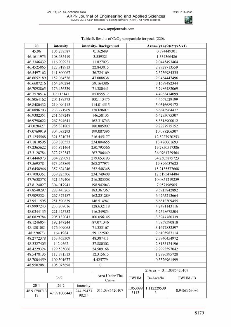
Table-3. Results of CeO2 nanoparticle for peak (220).
2θ intensity intensity- Background Area=(y1+y2)/2*(x2-x1)
45.96 105.238587 0.162689 0.374449301
46.1611973 108.635419 3.559521 1.334366486
46.3346432 116.902921 11.827023 2.0445493464
46.4525865 127.918913 22.843015 2.8928713559
46.5497162 141.800067 36.724169 2.3236984335
46.6052189 152.084536 47.008638 2.9464447496
46.6607216 164.240284 59.164386 3.1699482344
46.7092865 176.456339 71.380441 3.7986482069
46.7578514 190.13141 85.055512 4.4963474099
46.8064162 205.189373 100.113475 4.4567529199
46.8480432 219.090413 114.014515 5.0516689172
46.8896703 233.771969 128.696071 6.6843964477
46.9382351 251.657248 146.58135 6.4293075307
46.9798622 267.394641 162.318743 8.3318900012
47.028427 285.881805 180.805907 9.2227975152
47.0769919 304.083293 199.007395 10.088206307
47.1255568 321.521075 216.445177 12.5227920253
47.1810595 339.880553 234.804655 13.476061693
47.2365622 355.871464 250.795566 19.7850517386
47.3128784 372.782347 267.706449 36.0761729564
47.4446973 384.729091 279.653193 34.2505875723
47.5695784 373.953869 268.877971 19.896637623
47.6458946 357.624246 252.548348 15.2135577668
47.7083351 339.825306 234.749408 12.5195474484
47.7638378 321.459406 216.383508 10.0851219259
47.8124027 304.017941 198.942043 7.957196905
47.8540297 288.443265 183.367367 9.5913842892
47.9095324 267.327187 162.251289 6.4265213664
47.9511595 251.590839 146.514941 6.6812309455
47.9997243 233.708016 128.632118 4.2491143116
48.0344135 221.425752 116.349854 5.2548678504
48.0829784 205.132043 100.056145 3.8947780339
48.1246054 192.147244 87.071346 4.3959390818
48.1801081 176.409065 71.333167 3.1677832597
48.228673 164.1984 59.122502 2.6105987114
48.2772378 153.463309 48.387411 2.3940454972
48.3327405 142.9562 37.880302 2.8135124196
48.4229324 129.585066 24.509168 2.2993597042
48.5478135 117.391513 12.315615 1.2776395728
48.7004459 109.501677 4.425779 0.5526961499
48.9502081 105.075898 0
Σ Area = 311.0385420107
Io/2 Area Under The
Curve FWHM B=Area/Io FWHM / B
2θ-1 2θ-2 intensity
311.0385420107 1.053099
3113
1.112229539
3 0.9468363086 46.91790713
17 47.971006443
244.89473
98214

VOL. 13, NO. 20, OCTOBER 2018 ISSN 1819-6608
ARPN Journal of Engineering and Applied Sciences ©2006-2018 Asian Research Publishing Network (ARPN). All rights reserved.
www.arpnjournals.com
8180
Table-4. Results of CeO2 nanoparticle for peak (311).
2θ intensity intensity-Background Area=(y1+y2)/2*(x2-x1)
55.13721 114.31044 0.07067 0.1028394737
55.23146 116.35137 2.1116 0.2488311675
55.30371 119.01623 4.77646 0.5835202474
55.3854 123.74952 9.50975 1.073036286
55.46708 131.00417 16.7644 1.14322611
55.52363 137.90777 23.668 1.382093218
55.5739 145.55857 31.3188 1.4294008168
55.61474 152.92101 38.68124 1.4590072512
55.6493 159.99182 45.75205 2.0597680546
55.69014 169.35785 55.11808 2.4642741648
55.73098 179.80113 65.56136 2.4323096448
55.76554 189.43707 75.1973 3.0474005185
55.80324 200.70828 86.46851 3.796274032
55.84408 213.68086 99.44109 4.6952595006
55.88806 228.31662 114.07685 5.3474789424
55.93204 243.34068 129.10091 7.3822345961
55.98545 261.57528 147.33551 9.9005233271
56.04828 282.057 167.81723 13.462415148
56.12368 303.51578 189.27601 18.0892030751
56.21479 322.04867 207.8089 22.6194666761
56.32161 329.93708 215.69731 19.3615554245
56.41271 323.60405 209.36428 20.0600197985
56.51325 303.92104 189.68127 12.9677861925
56.5855 283.52836 169.28859 10.4632842367
56.65148 262.11651 147.87674 7.0028055449
56.70175 244.97077 130.731 5.4187093902
56.74573 229.92575 115.68598 5.3935785204
56.79599 213.18087 98.9411 2.9512620622
56.82741 203.15749 88.91772 3.6191071632
56.87139 189.90173 75.66196 2.4478046208
56.90595 180.23317 65.9934 2.304806088
56.94365 170.51725 56.27748 2.2512741882
56.98763 160.33947 46.0997 1.5925390455
57.02533 152.6249 38.38513 1.5160667411
57.06932 144.78243 30.54266 1.4194543366
57.12273 136.85024 22.61047 1.1408872026
57.18242 129.85638 15.61661 0.903721785
57.25467 123.63968 9.39991 0.5078771712
57.32379 119.53538 5.29561 0.3122495624
57.40861 116.3068 2.06703 0.100664361
57.50601 114.23977 0
Σ Area = 204.4540156863
Io/2 Area Under The
Curve FWHM B=Area/Io FWHM / B
2θ-1 2θ-2 intensity
204.4540156863 0.8993001555 0.9478746661 0.9487542897 55.869751166
4 56.7690513219
222.0738331
344

VOL. 13, NO. 20, OCTOBER 2018 ISSN 1819-6608
ARPN Journal of Engineering and Applied Sciences ©2006-2018 Asian Research Publishing Network (ARPN). All rights reserved.
www.arpnjournals.com
8181
Table-5. Results of CeO2 nanoparticle for peak (222).
2θ intensity intensity-background Area=(y1+y2)/2*(x2-x1)
67.8018922 90.1357243 0 0.0233960908
67.9759961 90.4044844 0.2687601 0.0789392671
68.1226099 90.9437969 0.8080726 0.1792136455
68.2600604 91.9353344 1.7996101 0.2701102251
68.3700207 93.2489823 3.113258 0.3138362526
68.452491 94.6333578 4.4976335 0.3592041266
68.5212162 96.0914362 5.9557119 0.399543292
68.5807781 97.5960818 7.4603575 0.5386915677
68.6449216 99.4718175 9.3360932 0.4620599058
68.6907384 100.969521 10.8337967 0.6494671761
68.7457186 102.927421 12.7916967 0.6933002219
68.7961171 104.85676 14.7210357 0.870393564
68.8510973 107.076762 16.9410377 0.8199709082
68.8969141 108.988147 18.8524227 1.1003395361
68.9518943 111.310058 21.1743337 1.227285904
69.0068745 113.606041 23.4703167 1.4688706857
69.0664363 115.987983 25.8522587 1.7334766335
69.1305799 118.333336 28.1976117 2.1502092325
69.2038868 120.601328 30.4656037 3.0314884782
69.3001021 122.684807 32.5490827 3.6270819723
69.4100625 123.557336 33.4216117 3.3324907119
69.5108595 122.836928 32.7012037 3.1911677237
69.6116565 120.753225 30.6175007 2.1627912256
69.6849634 118.524708 28.3889837 1.8652545165
69.7536886 116.028271 25.8925467 1.2544462683
69.8040871 114.024273 23.8885487 1.4466584516
69.8682306 111.354114 21.2183897 1.1027593522
69.9232108 109.032116 18.8963917 0.7436708926
69.9644459 107.309132 17.1734077 0.8828913057
70.0194261 105.079017 14.9432927 0.7635030934
70.0744063 102.966179 12.8304547 0.6011741831
70.1248048 101.162098 11.0263737 0.4705259249
70.1706216 99.6488001 9.5130758 0.5138483377
70.2301835 97.8769113 7.741187 0.4435297529
70.294327 96.2238342 6.0881099 0.4096338943
70.3722156 94.5660701 4.4303458 0.3511704457
70.4684309 93.0050584 2.8693341 0.2559442308
70.582973 91.7353886 1.5996643 0.1691793883
70.7341685 90.7739492 0.6382249 0.0642694818
70.8945273 90.2990704 0.1633461 0.0101599616
71.0182327 90.1366388 0.0009145
Σ Area = 40.0319478284
Io/2 Area Under
The Curve FWHM B=Area/Io FWHM / B
2θ-1 2θ-2 intensity 40.0319478284 1.1295267718 1.1977862764 0.9430119497
68.8468118196 69.9763385914 106.8480983669

VOL. 13, NO. 20, OCTOBER 2018 ISSN 1819-6608
ARPN Journal of Engineering and Applied Sciences ©2006-2018 Asian Research Publishing Network (ARPN). All rights reserved.
www.arpnjournals.com
8182
The silicon standard of x- ray diffraction pattern
was used as instrumental broadening for calibration with
the CeO2 nanoparticle pattern, the reason for chosen this
standard was the intensities values are more acceptable
with CeO2 intensities, also the integral breath of the
standard was estimated additional to the CeO2 integral
breaths for Voigt function calibration.
After calculate the FWHM and integral breadth
for all peaks as B h(x) and the standard pattern B g(x) from
the equation. (3) also testing these profiles for
clarification either Gaussian profiles or Lorentz profiles
by the equation. (9) and equation. (10) the results of
introduce that the peaks (111), (200), (220), (311) and
(222) were Gaussian profiles, after that for calibration the
Gaussian profile equation. (2b) used to determine the
integral breadth of sample profile B f(x), there for the
crystallite size <D> and the apparent strain η was estimating in this study according to the equation. (5) and
equation. (7) with the plot according to Williamson hall
equation. (15), the results included in the tables below:
Table-6. Results of silicon standard XRD pattern for the highest peak.
2θ intensity intensity-Background Area=(y1+y2)/2*(x2-x1)
28.2907574 929.244335 0 0.5095278101
28.3055275 998.238832 68.994497 0.8537563022
28.3129126 1091.46033 162.215995 0.6530475831
28.3162695 1156.10611 226.861775 1.1175217334
28.3202977 1257.23174 327.987405 0.993173376
28.3229832 1340.91314 411.668805 1.237018253
28.3256687 1438.83284 509.588505 1.5200495969
28.3283542 1551.69798 622.453645 1.3489959826
28.3303683 1646.34283 717.098495 1.5481825068
28.3323824 1749.49007 820.245735 2.4045416338
28.3350679 1899.75759 970.513255 2.8260796409
28.3377534 2063.4264 1134.182065 3.2808784673
28.3404388 2238.55558 1309.311245 3.7630941229
28.3431243 2422.46083 1493.216495 4.2641831121
28.3458098 2611.73673 1682.492395 6.0472886463
28.3491667 2849.65262 1920.408285 6.8339530791
28.3525235 3080.54308 2151.298745 9.1776390311
28.3565518 3334.52729 2405.282955 10.1175395472
28.36058 3547.3165 2618.072165 14.5817957626
28.365951 3740.99744 2811.753105 15.2781790407
28.37132 3808.74809 2879.503755 15.2898564857
28.3766929 3741.21315 2811.968815 14.5834542737
28.3820639 3547.71837 2618.474035 10.1193719552
28.3860921 3335.03521 2405.790875 9.1795995418
28.3901203 3081.12167 2151.877335 6.836150361
28.3934772 2850.26185 1921.017515 6.0491636853
28.396834 2612.35199 1683.107655 4.2658205017
28.3995195 2423.065 1493.820665 3.7646854965
28.402205 2239.13657 1309.892235 3.2825165262
28.4048905 2063.97435 1134.730015 2.8274967927
28.407576 1900.26505 971.020715 2.4058432017
28.4102615 1749.95194 820.707605 1.5490763443
28.4122756 1646.76854 717.524205 1.3498162752
28.4142897 1552.08682 622.842485 1.521028126
28.4169752 1439.17275 509.928415 1.2378675692
28.4196607 1341.20575 411.961415 0.9938624985
28.4223461 1257.47991 328.235575 0.9571534341
28.425703 1171.26908 242.024745 0.8144762192

VOL. 13, NO. 20, OCTOBER 2018 ISSN 1819-6608
ARPN Journal of Engineering and Applied Sciences ©2006-2018 Asian Research Publishing Network (ARPN). All rights reserved.
www.arpnjournals.com
8183
28.4297312 1091.60677 162.362435 0.7379626021
28.4357736 1011.14332 81.898985 0.5895722665
28.449201 935.161646 5.917311
Σ Area = 176.7112193845
Io/2 Area Under The
Curve FWHM B=Area/Io 2W / B
2θ-1 2θ-2 intensity
176.7112193845 0.057987114 0.0613686365 0.9448981961 28.342340591 28.400327705
2368.99
62125
Table-7. Calculation of B2f G.
Peak B h G B2 h G B g G (Standard) B
2g G B
2f G= B
2h G- B
2g G
111 0.9096677334 0.8274953852 0.0613686365 0.0037661096 0.8237292756
200 0.8892067286 0.7906886062 0.0613686365 0.0037661096 0.7869224967
220 1.1122295393 1.2370545481 0.0613686365 0.0037661096 1.2332884385
311 0.9478746661 0.8984663826 0.0613686365 0.0037661096 0.894700273
222 1.1977862764 1.4346919639 0.0613686365 0.0037661096 1.4309258543
Table-8. Results that used to plot B cos θ against sin θ.
Peak 2θ θ B Sin θ Cos θ B Cos θ
111 28.3233 14.16165 0.9075953259 0.2446584485 0.9696093252 0.8800128915
200 32.90292 16.45146 0.8870865215 0.2832029473 0.9590600037 0.8507692026
220 47.4446973 23.72234865 1.1105352036 0.4023049072 0.9155057409 1.0167013544
311 56.32161 28.160805 0.9458859725 0.4719477707 0.8816265092 0.8339181481
222 69.4100625 34.70503125 1.1962131308 0.5693517152 0.8220940484 0.9833996954

VOL. 13, NO. 20, OCTOBER 2018 ISSN 1819-6608
ARPN Journal of Engineering and Applied Sciences ©2006-2018 Asian Research Publishing Network (ARPN). All rights reserved.
www.arpnjournals.com
8184
0.2 0.3 0.4 0.5 0.6
0.80
0.85
0.90
0.95
1.00
1.05
B C
os
Sin
Figure-12. Relation between B cos θ and sin θ.
Table-9. Results of crystallite size and apparent strain by the plot.
the intercept 1 2 The Slope (η) K λ <L>vol= Kλ / the intercept
<D>= 4/3
<L>vol
0.838641686 X=0.350745946;
Y=0.897555621
X=0.499762162;
Y=0.95581089 0.0068195988 0.89
0.15406
nm 9.3723028 12.49640373
Also by the separation Double Voigt method the
crystallite size and the apparent strain could be obtained
by using the equation. (4) and equation. (5) and equation.
(6), the results in the table below:
Table-10. Results of crystallite size and apparent strain by separation double Voigt method.
Peak 2θ θ B Cos θ B Cos θ tanθ
111 28.3233 14.16165 0.9075953259 0.9696093252 1.102932598 0.2523268311
200 32.90292 16.45146 0.8870865215 0.9590600037 1.0662810692 0.2952922092
220 47.4446973 23.72234865 1.1105352036 0.9155057409 1.2742461809 0.4394346088
311 56.32161 28.160805 0.9458859725 0.8816265092 1.0451614043 0.5353148593
222 69.4100625 34.70503125 1.1962131308 0.8220940484 1.2325087409 0.6925627504
K λ <L>vol= K λ / B Cos θ <D>= 4/3 <L>vol η = B / tanθ
0.89 0.15406 nm
7.1228460823 9.4971281098 0.0627778134

VOL. 13, NO. 20, OCTOBER 2018 ISSN 1819-6608
ARPN Journal of Engineering and Applied Sciences ©2006-2018 Asian Research Publishing Network (ARPN). All rights reserved.
www.arpnjournals.com
8185
7.367681338 9.8235751174 0.0524313885
6.1652287071 8.2203049428 0.0441078044
7.5165606979 10.0220809305 0.0308394663
6.3740068319 8.4986757758 0.0301457993
Average: 6.9092647315 Average: 9.2123529753 Average: 0.0440604544
Scherrer method
According to Scherrer formula the crystallite size
of cerium oxide nanoparticle in (nm) and the lattice strain
were estimated by using equation. (11) and equation. (12)
and the results in tables below:
Table-11. Calculating the B and Cot θ from peaks.
Peak 2θ θ B Cos θ Cot θ
111 28.3233 14.16165 0.014796192 0.9696093252 3.9631140118
200 32.90292 16.45146 0.0146778661 0.9590600037 3.3864760692
220 47.4446973 23.72234865 0.0183800503 0.9155057409 2.2756514391
311 56.32161 28.160805 0.0156957487 0.8816265092 1.8680594844
222 69.4100625 34.70503125 0.0197139612 0.8220940484 1.4439124821
Table-12. Estimating crystallite size and lattice strain for Scherrer formula.
K λ <D>V = (K λ /B) Cos θ η = B Cot θ εͤ= η / 4
0.89 0.15406 nm
8.9851788259 0.0586389959 0.014659749
8.9590664354 0.0497062424 0.0124265606
6.8295843913 0.041826588 0.010456647
7.7016274082 0.0293205922 0.007330148
5.7177808756 0.0284652346 0.0071163086
Average= 7.6386475873
Average=
0.0415915306
Average=
0.0103978827
Size-strain plot (SSP) method
The crystallite size and the lattice strain were
calculated by using the plot, by using the equation. (16)
which the slope of the plot gives the crystallite size in
(nm) and the intercept with y- axis gives the root mean
square of the strain, the results are in the tables:
Table-13. Calculation used for the size-strain plot.
Peak 2θ θ B Cos θ Sin θ d=λ /2 Sin θ (d. B. Cos
θ)2 (d2. B .Cos θ)
111 28.3233 14.16165 0.0158405267 0.9696093252 0.2446584485 0.3148470878 2.34E-005 0.0015225297
200 32.90292 16.45146 0.0154825806 0.9590600037 0.2832029473 0.2719957569 1.63E-005 0.0010985337
220 47.4446973 23.72234865 0.0193824958 0.9155057409 0.4023049072 0.1914716888 1.15E-005 6.51E-004
311 56.32161 28.160805 0.0165088246 0.8816265092 0.4719477707 0.1632172134 5.64E-006 3.88E-004
222 69.4100625 34.70503125 0.0208778577 0.8220940484 0.5693517152 0.1352942266 5.39E-006 3.14E-004
VOL. 13, NO. 20, OCTOBER 2018 ISSN 1819-6608
ARPN Journal of Engineering and Applied Sciences ©2006-2018 Asian Research Publishing Network (ARPN). All rights reserved.
www.arpnjournals.com
8186
0.0000 0.0005 0.0010 0.0015
0.000005
0.000010
0.000015
0.000020
0.000025
(d.
B.
Co
s)
2
(d2. B. Cos)
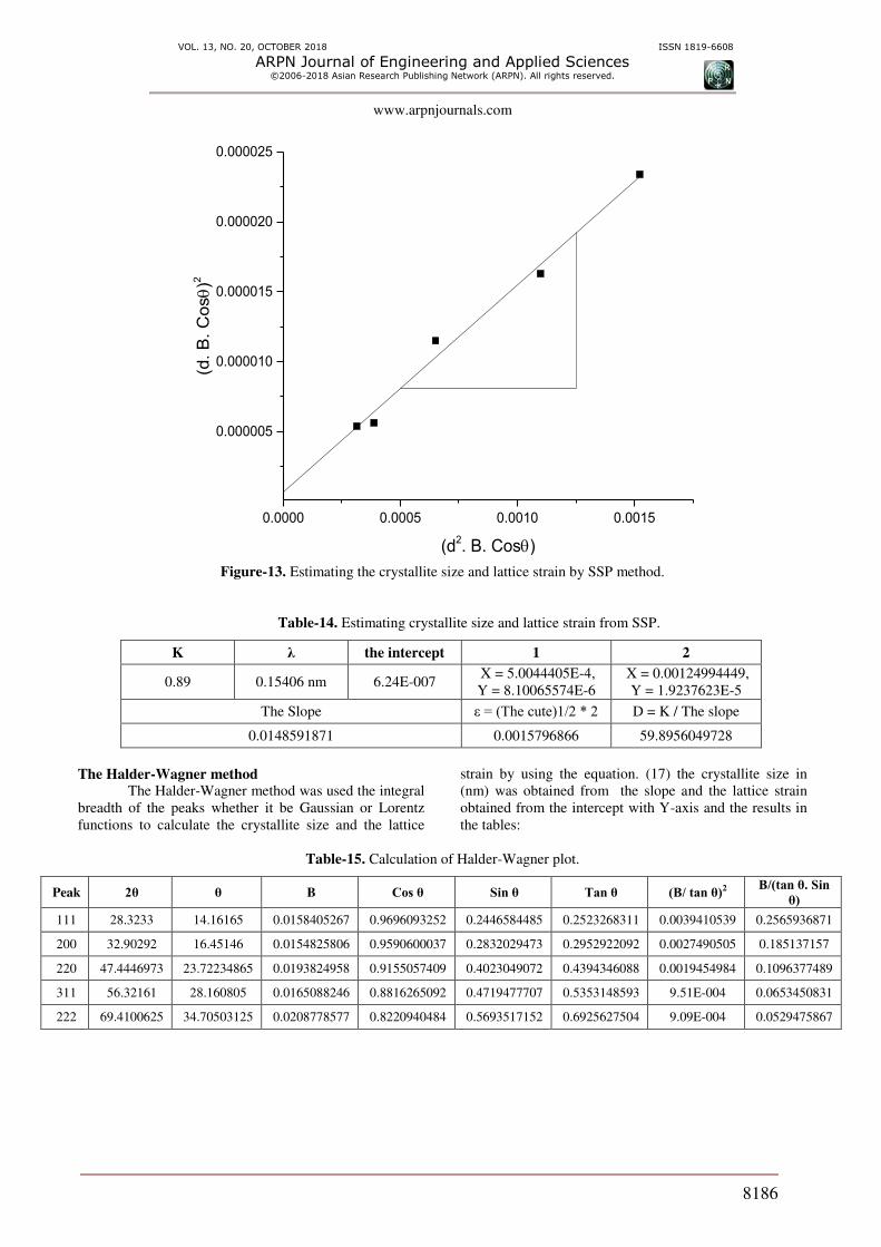
Figure-13. Estimating the crystallite size and lattice strain by SSP method.
Table-14. Estimating crystallite size and lattice strain from SSP.
K λ the intercept 1 2
0.89 0.15406 nm 6.24E-007 X = 5.0044405E-4,
Y = 8.10065574E-6
X = 0.00124994449,
Y = 1.9237623E-5
The Slope ε = (The cute)1/2 * 2 D = K / The slope
0.0148591871 0.0015796866 59.8956049728
The Halder-Wagner method The Halder-Wagner method was used the integral
breadth of the peaks whether it be Gaussian or Lorentz
functions to calculate the crystallite size and the lattice
strain by using the equation. (17) the crystallite size in
(nm) was obtained from the slope and the lattice strain
obtained from the intercept with Y-axis and the results in
the tables:
Table-15. Calculation of Halder-Wagner plot.
Peak 2θ θ B Cos θ Sin θ Tan θ (B/ tan θ)2 B/(tan θ. Sin
θ) 111 28.3233 14.16165 0.0158405267 0.9696093252 0.2446584485 0.2523268311 0.0039410539 0.2565936871
200 32.90292 16.45146 0.0154825806 0.9590600037 0.2832029473 0.2952922092 0.0027490505 0.185137157
220 47.4446973 23.72234865 0.0193824958 0.9155057409 0.4023049072 0.4394346088 0.0019454984 0.1096377489
311 56.32161 28.160805 0.0165088246 0.8816265092 0.4719477707 0.5353148593 9.51E-004 0.0653450831
222 69.4100625 34.70503125 0.0208778577 0.8220940484 0.5693517152 0.6925627504 9.09E-004 0.0529475867

VOL. 13, NO. 20, OCTOBER 2018 ISSN 1819-6608
ARPN Journal of Engineering and Applied Sciences ©2006-2018 Asian Research Publishing Network (ARPN). All rights reserved.
www.arpnjournals.com
8187
0.0 0.1 0.2 0.3
0.001
0.002
0.003
0.004
(B /
ta
n)
2
B / (tan. Sin)
Figure-14. Halder-Wagner relation between (B / tan θ) 2 and B/(tan θ. Sin θ).
Table-16. Estimating the crystallite size and lattice strain by Halder-Wagner plot.
K λ The intercept 1 2
0.89 0.15406 nm 1.14E-004 X = 0.100643872,
Y = 0.00160337705
X = 0.250111012,
Y = 0.00382404098
The slope ε= (the intercept /16)1/2 D = K λ / the slope
0.0148572049 0.0026704209 9.2287479779
CONCLUSIONS
a) The accuracy of the results given by the Voigt
method for the crystallite size and lattice strain, because it
depends on the analysis of the line of diffraction fully
where the line tails into the calculations.
b) The calculation of crystallite size and lattice
strain in the Sherrer method is very important because this
method gives the values of crystallite size and lattice
strain quickly. But the calculations in this method are
inaccurate because they depend on FWHM and not the
integral breadth of the peaks.
c) The use of other methods in the calculations to
demonstrate the validity of the results given by the
method used in the study through the implementation of
the method of Double Voigt and already found that there
is a high accuracy in the calculation of crystallite size and
lattice strain in relation to the ratio of other methods,
which each method is specific in the calculation of
crystallite size and lattice strain.
REFERENCES
[1] B. D. Cullity. 1956. Elements of X-Ray Diffraction,
Notre Dame, Indiana: Add1son-Wesley. p. 1.
[2] SIMM Thomas H. 2012. The Use of Diffraction Peak
Profile Analysis in Studying the Plastic Deformation
of Metals. School of Materials, University of
Manchester, Manchester.
[3] Thomas, P. Bindu Sabu. 2014. Estimation of lattice
strain in ZnO nanoparticles: X-ray peak. J Theor Appl
Phys. 8: 123-134.
[4] A. Cervellino, C. Giannini, A. Guagliardi and M.
Ladisa. 2005. Nanoparticle size distribution
estimation by a full-pattern powder diffraction
analysis. Phys. Rev. B. 72(3): 035412.
[5] Y. T. Prabhu, K. Venkateswara Rao, V. Sesha Sai
Kumar, B. Siva Kumari. 2013. X-ray Analysis of Fe
doped ZnO Nanoparticles by Williamson-Hall and

VOL. 13, NO. 20, OCTOBER 2018 ISSN 1819-6608
ARPN Journal of Engineering and Applied Sciences ©2006-2018 Asian Research Publishing Network (ARPN). All rights reserved.
www.arpnjournals.com
8188
Size-Strain Plot. International Journal of Engineering
and Advanced Technology (IJEAT). 2(4): 268-274.
[6] J. I. Langford. 1978. A Rapid Method for Analysing
the Breadths of Diffraction and Spectral Lines using
the Voigt. J. Appl. Cryst. 11: 10-14.
[7] J. I. Langford. 1992. The Use of the Voigt Function in
Determining Microstructural Properties from. in
Accuracy in Powder Diffraction II, Gaithersburg.
[8] S. Vives, E. Gaffet, C. Meunier. 2004. X-ray
diffraction line profile analysis of iron ball milled
powders. Materials Science and Engineering. A366:
229-238.
[9] Meier Mike L. 2005. Measuring Crystallite Size
Using X-Ray Diffraction, the Williamson-Hall
Method. University of California, Davis, California.
[10] H. G. Jiang, M. Rühle and E. J. Lavernia. 1999. On
the applicability of the x-ray diffraction line profile
analysis in extracting grain size and microstrain in
nanocrystalline materials. Journal of Materials
Research. 14(2): 549-559.
[11] Xiaolu Pang, Kewei Gao, Fei Luo, Yusuf Emirov,
Alexandr A. Levin, Alex A. Volinsky. 2009.
Investigation of microstructure and mechanical
properties of multi-layer Cr/Cr2O3 coatings. Thin
Solid Films. 517(6): 1922-1927.
[12] Parviz Pourghahramani, Eric Forssberg. 2006.
Microstructure characterization of mechanically
activated. International Journal of Mineral Processing.
79(2): 106-119.
[13] K. Venkateswarlu, A. Chandra Bose, N.Rameshbabu.
2010. X-ray
peakbroadeningstudiesofnanocrystallinehydroxyapatit
e. Physica B: Condensed Matter. 405(20): 4256-4261.
[14] Farrukh, Sadia Perveen Muhammad Akhyar. 2017.
Influence of lanthanum precursors on the
heterogeneous La/SnO2-TiO2 nanocatalyst with
enhanced catalytic activity under visible light. Journal
of Materials Science: Materials in Electronics. 28(15):
10806-10818.
[15] B. Rajesh Kumar, B. Hymavathi. 2017. X-ray peak
profile analysis of solid-state sintered alumina doped
zinc. Journal of Asian Ceramic Societies. 5(2): 94-
103.
[16] Xin Guo, Christopher McCleese, Charles Kolodziej,
Anna C. S. Samia, Yixin Zhao and Clemens Burda.
2016. Identification and characterization of the
intermediate phase in hybrid organic–inorganic
MAPbI3 perovskite. Dalton Trans. 45(9): 3806-3813.


