Policy Research Working Paper 5826

DR-CAFTA and the EnvironmentBárbara Cunha

Muthukumara Mani

The World BankLatin America and the Caribbean RegionPoverty Reduction and Economic Management UnitOctober 2011

WPS5826P

ublic

Dis

clos

ure

Aut

horiz

edP

ublic

Dis

clos

ure

Aut

horiz

edP

ublic

Dis

clos

ure

Aut

horiz

edP

ublic

Dis

clos

ure

Aut

horiz

edP

ublic

Dis

clos

ure

Aut

horiz

edP

ublic

Dis

clos

ure

Aut

horiz

edP

ublic

Dis

clos

ure

Aut

horiz

edP

ublic

Dis

clos

ure

Aut

horiz

ed

Produced by the Research Support Team

Abstract

The Policy Research Working Paper Series disseminates the findings of work in progress to encourage the exchange of ideas about development issues. An objective of the series is to get the findings out quickly, even if the presentations are less than fully polished. The papers carry the names of the authors and should be cited accordingly. The findings, interpretations, and conclusions expressed in this paper are entirely those of the authors. They do not necessarily represent the views of the International Bank for Reconstruction and Development/World Bank and its affiliated organizations, or those of the Executive Directors of the World Bank or the governments they represent.

Policy Research Working Paper 5826

The Dominican Republic-Central American Free Trade Agreement with the United States aims to create a free trade zone for economic development. The Agreement is expected to intensify commerce and investment among the participating countries. This paper analyzes the changes in the production and trading patterns in 2-digit manufacturing sectors with the goal of understanding the short-term environmental implications of the Dominican Republic-Central American Free Trade Agreement. More specifically, the paper addresses the questions:

This paper is a product of the Poverty Reduction and Economic Management Unit, Latin America and the Caribbean Region. It is part of a larger effort by the World Bank to provide open access to its research and make a contribution to development policy discussions around the world. Policy Research Working Papers are also posted on the Web at http://econ.worldbank.org. The authors may be contacted at bcunha@worldbank.org and mmani@worldbank.org.

Did pollution increase in the period after the Agreement negotiations? Did trade and production shift toward pollution intensive factors? The results suggest an increase in pollution emissions in the post-negotiations period. The increase in emissions is mainly attributable to scale effects. Composition effects are small and in some cases (including Nicaragua and Honduras) favoring cleaner industries and partially compensating the pollution gains from output and export growth.

DR-CAFTA and the Environment

Bárbara Cunha and Muthukumara Mani

1

JEL: F18, F40, O44, Q5

Keywords: Trade, Environment, Trade Agreements, Pollution, Composition, Growth.

1 1This was prepared as a background paper for the report ―Getting the most out of Central America Trade

Agreements‖. Bárbara Cunha is a Economist in the Economic Policy Unit in the Latin America and the Caribbean

Region and Muthukumara Mani is a Senior Environmental Economist in Environment Water Resources and Climate

Change Unit in the South Asian Regions of the World Bank. We are grateful for comments received on an earlier

draft from Sushenjit Bandyopadhyay, J. Humberto lopez and Rashmi Shankar. We are also grateful to Teresa

Molina for the capable research assistance.

2

I. Introduction

The seminal work of Grossman and Krueger (1992) ignited a debate on the impact of international trade

on the environment. Originally fueled by negotiations over the North American Free Trade Agreement

(NAFTA), the debate remains relevant as new bilateral and multilateral agreements are formed and

environmental concerns continue to rise. This paper contributes to this recent literature by assessing the

environmental implications of trade, specifically the pollution effects of the changes in production and

trading patterns that followed the Dominican Republic–Central American Free Trade Agreement with the

United States (DR-CAFTA).

The DR-CAFTA promotes commercial and financial integration among member countries. The

agreement, passed by the US Congress on July 28, 2005, encompasses the United States and the Central

American countries of Costa Rica, El Salvador, Guatemala, Honduras, and Nicaragua, and the Dominican

Republic. DR-CAFTA’s main goal is to create a free-trade and investment zone for economic

development, and includes several measures to regulate investment activities and to facilitate the

exchange of goods and services. The Agreement has a complementary policy agenda addressing local

competitiveness, property rights, labor, and environmental issues. On the environmental side, the

Agreement emphasizes the monitoring and implementation of current environmental laws, but unlike

NAFTA it pays less attention to the strengthening and harmonizing of unequal environmental standards

among member countries.

The literature on trade and the environment discusses various channels through which trade liberalization

(and trade agreements) can affect pollution emissions. On the one hand, empirical evidence indicates that

trade liberalization can stimulate economic growth. Scaling up (holding constant the mix of goods

produced and production techniques) leads to an increase in pollution (scale effects). On the other hand,

trade liberalization changes relative prices by intensifying foreign competition. As a result, the structure

of production is expected to change according to relative comparative advantages—defined by both

factors of production and institutional arrangements. This effect can either increase or decrease relative

output in pollution-intensive sectors (composition effects). Finally, changes in production technologies

(including pollution intensity by unit of output) tend to follow trade liberalization (technique effects).

Technique effects can result from different forces: while trade facilitates the access to more efficient (and

cleaner) technologies, stronger competition can trigger a race to the bottom of environmental standards,

favoring the adoption of cheaper and dirtier technology in the short run. Nevertheless, as income grows,

the demand for environmental quality tends to increase. By adopting both tighter environment policies

and more advanced, cleaner technologies, countries can afford to reduce emissions after reaching a certain

level of income. This inverted-U relationship between per capita income and pollution is known as the

environmental Kuznets curve2.

Previous empirical studies on the relationship between trade and the environment have found varying

results. For example, Dean (2002) uses province-level data on water pollution from China and finds

support for the idea that trade liberalization has both a direct and an indirect effect on emissions growth

2 Its proponents argue that environmental degradation is just a matter of ―growing pains‖ that will disappear with prosperity.

3

and that these can be opposite in sign. In contrast, Grossman and Krueger (1992) examine the

environmental impacts of NAFTA and find no evidence that a comparative advantage is being created by

lax environmental regulations in Mexico. Using data for different countries from 1960 to 1995, Mani and

Wheeler (1998) find that ―pollution haven effects‖ are insignificant in developing countries. In a closely

related study, Gamper-Rabindran and Jha (2004) analyze the empirical relationship between trade

liberalization and the environment in the Indian context. Their findings indicate that exports and foreign

direct investment grew in the more polluting sectors relative to the less polluting sectors between the pre-

and post-liberalization periods. This evidence provides some support for concerns raised about the

environmental impact of trade liberalization.

This paper builds on this literature by assessing the pollution effects related to implementation of the DR-

CAFTA. It starts by revisiting the related literature and discussing the possible implications of the

agreement for Central America environmental conditions in the short and medium term. It then computes

the scale, composition, and technique effects of pollution by comparing average annual emissions before

and after implementation of the agreement3. The analysis shows, as often found in the literature, that the

scale effects outweigh the composition and technique effects. Most of the variation in pollution results

from a scaling up of production. Composition effects are small and vary in sign across member countries.

This result suggests that environmental regulation in most DR-CAFTA countries is not a major factor

influencing pollution dynamics. This idea is also supported by the findings of the second empirical

exercise. The second part of the analysis investigates whether the sectoral changes in production and

exports that followed the DR-CAFTA favored pollution-intensive (―dirty‖) industries. Consistent with the

results of the first exercise, this analysis indicates that the period following negotiation of the agreement

is associated with a slowdown in the relative growth and export of pollution-intensive industries.

The results indicate that all countries could benefit from closing the gaps in their environmental

regulatory framework in terms of regulations, capacity, and monitoring. Countries such as El Salvador,

where the agreement favored the relative expansion of more-polluting industries, should go beyond the

DR-CAFTA environmental agenda and work on strengthening regulations in the short run. However,

environmental reforms should be accompanied by a competitiveness agenda (including reforms to

facilitate training, access to credit, and logistics) that would help to compensate for the costs imposed by

the additional rigidity in the environmental laws. For poorer countries such as Nicaragua and Honduras,

environmental regulations do not seem to play an important role in the current allocation of production.

Nevertheless, as these economies grow, the situation will change. For this reason, these countries should

start planning and implementing a medium-term environmental agenda.

The remainder of this paper is organized as follows. Section II reviews the recent environmental

development is Central America. Section II revisit the trade and environment literature and discusses the

potential implication of the DR-CAFTA. Section IV outlines the basic exercise and presents the data,

while Section V presents the results of the analysis. A final section concludes with a discussion of the

results and their implications.

II. DR-CAFTA and the Environment

3 Data limitations prevent us from assessing technological changes directly, so we create an alternative scenario drawing from

results in the literature.

4

The main goal of DR-CAFTA was to create a free trade zone for economic development, regulate

investment activities, and facilitate the trade of goods and services. The agreement has a complementary

policy agenda addressing local competitiveness, property rights, labor, and environmental issues. Chapter

10 and specifically chapter 17 of the agreement outline the rules, regulations, and other provisions for

addressing environmental issues. Under chapter 17, each party shall, among other things, (a) ensure that

its laws and policies provide for and encourage high levels of environmental protection; (b) not fail to

effectively enforce its current environmental laws; (c) ensure that judicial, quasi-judicial, or

administrative proceedings are available to sanction or remedy violations of its environmental laws, that

such proceedings are fair, equitable and transparent, and that tribunals that conduct or review such

proceedings are impartial and independent; (d) provide appropriate and effective remedies or sanctions

for a violation of environmental laws; (e) ensure that interested persons have the right to request a party’s

competent authorities to investigate alleged violations of its environmental laws; and (f) encourage the

development and use of incentives and other flexible and voluntary mechanisms to protect or enhance the

environment.

In support of these obligations, the parties entered into a separate Environmental Cooperation Agreement

to protect, improve, and conserve the environment, including natural resources. The agreement establishes

the creation of a Dominican Republic–Central America–United States Environmental Cooperation

Commission composed of government representatives appointed by each party. The commission is

responsible for identifying priorities for cooperative activities and developing a program of work in

accordance with those priorities. It also examines and evaluates the cooperative activities under the

agreement and recommends ways to improve future cooperation. In addition, the U.S. administration

agreed to commit roughly US$40 million a year from fiscal 2006 to fiscal 2009 to help countries to

implement labor and environmental provisions. By the end of 2010, a total of $38.8 million has been

allocated to strengthen the capacity of members to comply with the environmental provisions of DR-

CAFTA and to build environmental capacity linked directly to trade in broad program areas, including

DR- CAFTA specific obligations.

Under DR-CAFTA, countries are mainly required to enforce their existing laws. Although the provision

prevents a race to the bottom among member countries, there is no explicit requirement for strengthening

existing regulatory frameworks. In addition, critics of the agreement point to the existence of loopholes in

that provision: ―Although DR-CAFTA establishes a citizen submission process to allege enforcement

failures, it does not provide for any clear outcomes or actions to actually ensure that citizens of the region

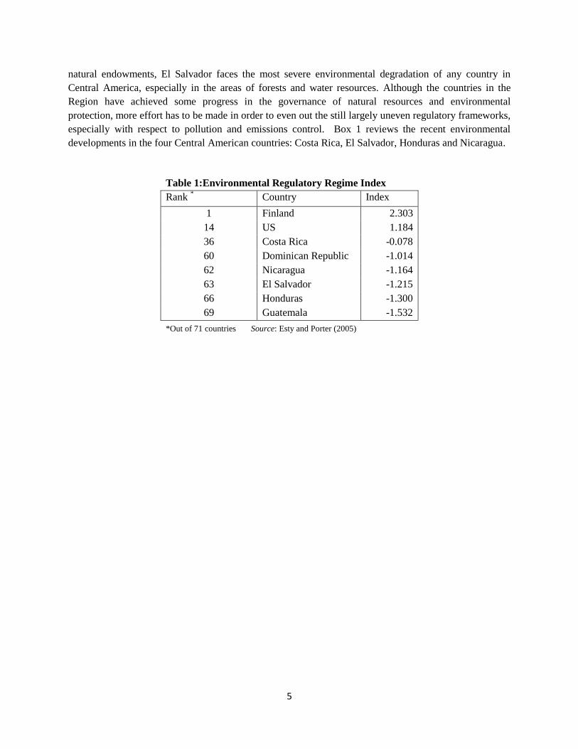
can achieve enforcement of environmental laws‖ (Sarkar 2009). Finally, existing environmental laws vary

significantly across member countries. Table 1 compares the ranking of select environmental regulatory

regimes during the DR-CAFTA negotiation period (following Esty and Porter 2005). While the

environmental regimes of the United States and Costa Rica score above the international average, those of

Guatemala and Honduras score among the bottom five. These differences could potentially favor the rise

of pollution havens within the region.

Given the new challenges following the signing of DR-CAFTA, we review the regulatory environmental

frameworks of countries to underline the differences among them. While Costa Rica has been a regional

leader on environmental issues, ensuring that economic growth is not achieved at the expense of its rich

5

natural endowments, El Salvador faces the most severe environmental degradation of any country in

Central America, especially in the areas of forests and water resources. Although the countries in the

Region have achieved some progress in the governance of natural resources and environmental

protection, more effort has to be made in order to even out the still largely uneven regulatory frameworks,

especially with respect to pollution and emissions control. Box 1 reviews the recent environmental

developments in the four Central American countries: Costa Rica, El Salvador, Honduras and Nicaragua.

Table 1:Environmental Regulatory Regime Index

Rank * Country Index

1 Finland 2.303

14 US 1.184

36 Costa Rica -0.078

60 Dominican Republic -1.014

62 Nicaragua -1.164

63 El Salvador -1.215

66 Honduras -1.300

69 Guatemala -1.532

*Out of 71 countries Source: Esty and Porter (2005)

6

Box 1. Regulatory and Institutional Framework

1. Costa Rica

Before the DR- CAFTA: Costa Rica has achieved significant progress in the development of institutions and organizations

since 1991. In 1995 the country passed a new General Environmental Law and created the Ministry of the Environment and

Energy. The Act established air as a common property and grants the state authority to protect the environment and prevent

and control pollution. It sets up guidelines, coordination mechanisms and the legal framework for the sustainable

exploitation of natural resources and for the protection of the environment. As an example, the law created the National and

Regional Environmental Councils, National Technical Secretariat for the Environment, the Administrative Environmental

Tribunal or the Environmental Comptroller's Office. Since then, a large number of institutions have been created in specific

areas related to environment and climate change, the Forestry Act in 1996 Establishes the state functions to ensure the

conservation, protection and proper management of forests, as well as the production, use and industrialization of forest

resources, the Biodiversity Act and the Land Use Management and Conservation Act (1998), the Environmental Services

Payment in 2000 established the FONAFIFO (National Fund for Forestry Financing) to pay for environmental services

rendered by forests and plantations, with funding from public and private institutions and it also set maximum payments for

reforestation and protection management plans.

After the DR- CAFTA: The environment program in Costa Rica is particularly ambitious and is one of the most developed

among emerging countries. The government aims to become carbon-neutral by 2021, although it still faces caveats related to

the increase in the energy costs and in the pressure of the population. Costa Rica should keep making efforts in fighting

deforestation, lost of biodiversity and desertification, meanwhile environmental institutions might strength controls and

evaluations.

2. El Salvador

Before DR-CAFTA: El Salvador has made substantial progress in building its institutional capacity to address environmental and

natural resource problems. In 1998 the country passed a new Environmental Law (LMA) and created the Ministry of the

Environment and Natural Resources. The LMA is the cornerstone of the country’s system of law and regulations in environment

and it entrusts the Council of Ministers with the country’s environmental policy. In 2000 the Council established the Política

Nacional del Medio Ambiente y Lineamientos Estrátegicos which is based on three overarching principles: Dynamic

Equilibrium, Shared Responsibility and Social Interest. The LMA sets out the roles and enforcement powers of the Ministry of

Environment and Natural Resources (MARN), the National Environmental Management System (SINAMA) and other

government institutions. The main tool of the LMA is a permitting system that requires Environmental Impact Assessments

for new projects. Besides the LMA, the government passed the Conservation of Wildlife Law (1999) and the Forestry Law

(2002). Under the LMA the country strengthened social participation by passing a law on access to information and

introducing a system to collect and manage environmental complaints; and promoted environmental education by introducing

environmental issues in programs and courses at all levels of the National Education System.

After DR-CAFTA: In 2004 the government launched a national development plan (Safe Country 2004-2009) to enhance growth

under the assumption of CAFTA adoption. It included the new environmental strategy of the government under the chapter

called ―Environment: Legacy for Future Generations‖, with three main pillars: Natural Resources Conservation, Integrated

Management of Water Resources and Integrated Management of Solid Wastes. The government created the National

Environment Commission (CONAMA) as a consultative body for the MARN and an Executive Environmental Committee

to ensure that CONAMA directives are followed. In 2005 the government passed the fourth and last environmental laws, the

Natural Protected Law. Since then, the government has created an Inspectoría Ambiental, a land development plan to

prevent and manage environmental risk and degradation. The MARN has developed sector agreements. To strength the

institutional capacity and to improve the environmental framework, the MARN and SINAMA have been under continuing

redefinition.

7

Despite this large list of accomplishments, there are apparent weaknesses in several areas with regard to

the efficiency and effectiveness of environmental and natural resource management policies, as pointed

out by Sarkar (2009). Areas of weakness include environmental information, environmental quality, and

institutional performance; coordination between environmental authorities and other sector agencies;

regulatory instruments; and compliance, monitoring, and enforcement mechanisms.

3. Honduras

Before DR-CAFTA: Honduras has developed a number of institutions and organizations to manage natural resources and

protect the environment, including the 1993 General Law for the Environment. This law establishes that protecting,

conserving, and managing the environment and natural resources is a matter of public interest and that the national

government and municipalities must promote rational use and sustainable management of these resources In 1996, during

the government modernization process, Environment Secretariat and the Natural Resources Secretariat were merged into a

single Environment and Natural Resources Secretariat (SERNA). Honduras has signed more than 60 international

environmental conventions, protocols, and treaties addressing regional and global.

After DR-CAFTA: The country’s legal and regulatory frameworks have been strengthened to address, among other issues:

management of water resources, protected areas, and forests; land use planning; pollution prevention; environmental health;

and rural development. Recently issued national policies related to the environment include: Honduras Environmental Policy

(2005); Agriculture and Rural Environment, which contains sections on Forestry and Productive Development, Forestry and

Community Development, and Forestry and Biodiversity (2004); Action Plan for a Sustainable Energy Policy (2005);

Environmental Mainstreaming (2005); and Simplification and Decentralization of Environmental Management, which

included licensing (2002). Forest and Protect Area Act is under discussion in third debate, reforms of the National law on

mines, law on incentives for the use of renewable energy, and the legislation on water resources are planned in the actual

congress. In addition, the National System of Environmental Information (SINIA), created in 1993, is responsible for

developing databases, websites, geographic information systems, remote sensing, and indicators.

4. Nicaragua

Before DR-CAFTA: In 1994 the Ministry of the Environment and Natural Resources (MARENA) was created to accomplish

the formulation, coordination and enforcement of environmental policy. Two years later the government passed the General

Law on Environment and Natural Resources which became the cornerstone of the environmental legal and regulatory

framework. It is in charge of administering the National Protected Areas System, administering Environmental Impact

Assessment (EIA), coordinating the National Environmental Information System (SINIA) and coordinating disaster

prevention and response measures jointly with the National System for Disaster Prevention, Mitigation and Response

(SINAPRED). Two regional environmental agencies (SERNA) were building to be in charge of environmental policy

functions in the north and south Atlantic regions. Since MERNA was established the government has passed the Law on

Exploration of Geothermal Resources in 2002 and one year later the Law on the Promotion of Hydropower and on Citizen

Participation.

After DR-CAFTA: In 2006 the government passed the Law on Forest Felling Ban. Related to the water legislation, in 2007

the National Council on Potable Water and Sanitation (CONAPAS) approved a 10 year comprehensive sector strategy for

the country's water and in 2008 the National Water Law was passed by the government. The Ministry of Natural Resources

(MARENA) has developed environmental policies in eleven areas: conservation of water sources, pastures, productive use

of water, protected areas, sustainable forestry, national reforestation campaign, sustainable land management, control and

reduction of contamination, solid waste management, mitigation and adaptation to climate change, and environmental

education. Recent acceptance of Nicaragua in the pilot group of countries for financing activities to reduce deforestation

through the Forest Carbon Partnership Facility (FCPF) is a major opportunity to enhance the policies and mechanisms for

forest governance.

8

Increased trade can lead to different kinds of environmental pressures. Trade-related production

specialization, linked to the reallocation of productive resources, can create additional environmental

pressures. One of the main environmental problems faced by Central American countries, not addressed

in this study, is deforestation. Future research on the topic should take into account differences in the

scope of and compliance with deforestation laws, for example, in Costa Rica and Honduras, because the

expansion of agricultural frontiers in less protected countries could have a role in deteriorating watersheds

and decreasing biodiversity. Although beyond the scope of this paper, climate change also could

exacerbate existing conditions in some countries.

III. Trade and the Environment: A Review of the Literature

A few concerns are frequently present in the debate over trade liberalization and environmental policy.

First, there is concern that reducing barriers to trade could reinforce the creation of pollution havens. In

places with weak environmental policies, trade liberalization may shift the composition of production and

exports to more pollution- or resource-intensive sectors. Second, trade liberalization may directly affect

environmental standards by encouraging a race to the bottom. While the risks of a race to the bottom in

environmental standards are reduced by the environmental clauses in the DR-CAFTA, regulatory

differences between countries could potentially play a role in the production and export of pollution-

intensive commodities.

The political debate has been followed by an effort in the economic literature to search for theoretical

underpinnings and empirical evidence to justify such concerns. On the theoretical side, works can be

divided into two main groups. The first group focuses on the direct relationship between trade and the

environment, and most works extend the traditional trade framework to account for pollution modeled as

an input or a second output of production (Copeland and Taylor 1994; Antweiler, Copeland, and Taylor

2001; Péridy 2006; Di Maria and Smulders 2004). The second group focuses on an indirect relationship

between trade and pollution, in particular, the relationship between economic growth (facilitated by

international trade, among other things) and pollution (Stokey1998; Copeland and Taylor 2003). On the

empirical side, many papers attempt to assess the relationship between trade, growth, and the

environment. While early works focus on testing the pollution havens hypothesis, later works try to

disentangle the channels through which these variables interact (Cole and Rayner 2000; Grether, Mathys,

and de Melo 2009). Copeland and Taylor (2004) provide a comprehensive review of both theoretical and

empirical work on the topic. This section focuses on select study that will serve as base for assessing the

expected effects of the trade agreement on pollution in Central America.

Copeland and Taylor (1994), in what is considered a seminal work in the trade and environment literature,

develop a two-country static general equilibrium model of international trade to explain the pollution

haven hypothesis. The authors focus on how differences in human capital across countries affect their

income, regulation, trade flows, and pollution levels. Large differences in human capital across regions

ensure that each country specializes in a set of either relatively clean or dirty goods in trade. The intuition

for these results is fairly clear. Trade alters the composition of output in both countries with high and

countries with low human capital because of differences in the stringency of their pollution regulations.

Given the relative cost structure in autarky, a movement toward free trade shifts the production of dirty

9

goods to the country with lax regulation and the production of clean goods to the one with strict

regulation. However, the authors pay little attention to other factors that influence trade patterns and the

environmental effects resulting from them. For example, a simple factor endowment hypothesis suggests

that dirty capital-intensive processes should relocate to relatively capital abundant developed countries.

Antweiler, Copeland, and Taylor (2001) extend the previous framework to account for variables such as

factor costs and endowments and technological changes. The theoretical framework supports a model

based decomposition of the trade effect on emissions into scale, composition, and technique effects. Scale

effect relates to the scaling up (holding constant the mix of goods produced and production techniques) of

economic activity and inevitably leads to an increase in pollution emissions. The composition effect

measures the change in pollution resulting from changes in the production structure (all else equal). These

changes depend on the country’s comparative advantages – defined by both factors of production and

institutional arrangements. Finally, the technique effects assess the changes in production technologies

(including the pollution intensity by unit of output) that follow trade liberalization. Technique effects

have no clear sign and it can result from different forces. 4. According to their model, while trade

facilitates the adoption of more efficient (and cleaner) technologies of production, increased competition

could trigger a race to the bottom on environmental standards, favoring the adoption of cheaper or dirtier

technology in the short run. Nevertheless, as income grows, the demand for environmental quality tends

to increase. The author’s proxy the technique effect by a moving average of lagged income, representing

the slow transmission of income gains into abatement technologies.

Recent works have built on the framework of Antweiler, Copeland, and Taylor (2001), but the main

channels and effects remain similar. For example, Kahn and Yoshino (2004) consider trade among

different types of partners, including North-North, North-South, and South-South, and the formation of

trading blocks. The formation of trading blocs will most likely result in a shift toward dirtier industries in

the middle-income country, which is moderately capital abundant but still has a relatively weak

regulatory framework. These results reconcile the pollution haven and factor endowment hypotheses.

The relationship between economic development and environmental quality has been extensively

explored since Grossman and Krueger (1992) suggested an inverse-U relationship between income per

capita and pollution, the so-called environmental Kuznets curve (EKC). Most theoretical works agree

with the idea that economic development in low income countries is associated with industrialization and

a consequent increase in pollution, but they present different explanations for the declining portion of the

curve. Reasons for this inverted-U relationship include income-driven changes in (i) the composition of

production or consumption (Selden and Song 1994; Hettige, Mani, and Wheeler 2000; Brock and Taylor

2004); (ii) the preference for environmental quality (Stokey 1998); (iii) institutions dealing with

externalities (López 1994; Chichilnisky 1994); or (iv) increasing returns to scale associated with pollution

abatement (Bovenberg and Smulders 1995; Stokey 1998). Among the empirical studies, results seem

dependent on the type of pollution analyzed.

Many contributions have empirically tested the existence of an EKC using cross-country relationships

(among the others, Grossman and Krueger 1995; Stern, Common, and Barbier 1996), time-series analyses

4 Following the terminology proposed by Grossman and Krueger (1992).

10

for specific countries (Egli 2004), or panel data (Dijkgraaf and Vollebergh 2004; de Bruyn, van den

Bergh, and Opschoor 1998). While studies focusing on sulfur dioxide, nitrogen oxide, suspended

particulates, and an aggregate measure of air pollution tend to support the existence of an EKC

(Grossman and Krueger 1992; Markandya, Golub, and Pedroso- Galinato 2006), papers studying carbon

dioxide emissions (Aslanidis 2009) or water pollution are less conclusive (Hettige, Mani, and Wheeler

2000). The EKC may vary with country-specific characteristics, but studies supporting the EKC

hypothesis suggest that the turning point5. ranges from US$2,805 (Halkos 2003) to US$9,239 (Stern and

Common 2001) According to these studies, with the exception of Costa Rica, all countries in Central

America would currently be placed in transition or in the increasing part of the EKC6.

Empirical studies testing for the direct effects of trade on the environment are less conclusive. For

example, Gamper-Rabindran and Jha (2004) empirically analyze the relationship between trade

liberalization and the environment in the Indian context. Their findings indicate that exports and foreign

direct investment grew in the more-polluting sectors relative to the less-polluting sectors between the pre-

and post-liberalization periods. Mani and Jha (2006) and Akbostanci, Ipek Tunc, and Türüt-Asik (2004)

find similar results for Vietnam and Turkey, respectively. Dean (2002) supports the idea that trade

liberalization had both a direct and an indirect effect on emission growth in China and these effects could

be opposite in sign. In contrast to this works, Grossman and Krueger (1993) found no evidence that a

comparative advantage is being created by lax environmental regulations in Mexico. This result is also

confirmed by Stern (2005), who finds only small pollution effects of NAFTA on Mexico shortly after the

agreement, followed by an improvement in environmental quality afterwards. Gale and Mendez (1998)

suggests a strong link between capital abundance and pollution concentrations in production and trade

composition even after controlling for incomes per capita (supposed link to the country’s regulatory

framework). Finally, Melo, Grether and Mathys (2007) measures the aggregate effects of trade on

pollution taking into account a large sample of developed and developing countries. The author argue that

contrarily to concerns raised by environmentalists, an emission-decomposition exercise shows that scale

effects are dominated by technique effects working towards a reduction in emissions worldwide.

While data and methodological issues could help to explain the differences in findings, one interesting

pattern arises from the literature. Consistent with the predictions of Kahn and Yoshino (2004), positive

links between international trade and pollution are more frequently identified in studies dealing with

middle-income countries. These and a few other findings from the literature will help to guide discussion

of the possible and expected implications of DR-CAFTA for the environment in the Central America

economies.

Possible Environmental Developments for the DR-CAFTA

There are significant differences among DR-CAFTA countries. Countries differ not only in their

regulatory environments, but also in their level of development, income, and human and physical capital

endowments. Following the predictions of EKC theory, one would guess that, even before the agreement,

countries were likely to be experiencing different trends with respect to pollution emissions. Both level of

5 Defined as the level of income per capita (purchasing power parity, PPP) beyond which emissions start to decline. 6 Per capita GDP (US$, PPP) in 2009: Costa Rica, US$10,737; Dominican Republic, US$8,570; El Salvador, US$7,570;

Guatemala, US$4,873; Honduras, US$4,282; Nicaragua, US$2,668.

11

income and regulatory framework suggest that Costa Rica is experiencing a decline in pollution and that

Nicaragua, Honduras, and Guatemala are in the upward-sloping stages of the EKC. El Salvador and the

Dominican Republic have intermediary income levels, but weak regulatory frameworks. These countries

were probably approaching the turning point before the agreement.

As a consequence of these regional disparities, the medium-term environmental implications of the

agreement with the United States are likely to differ among member countries. Following the framework

proposed by Kahn and Yoshino (2004), one would expect that, at least in the medium term, countries like

Honduras, Guatemala, and Nicaragua would tend to specialize in labor-intensive products. Despite their

lax regulatory frameworks, these countries seem to have low comparative advantage in capital- intensive

industries7 (which correspond to approximately 4 percent of GDP, while the regional average is more than

7 percent). One would expect a negative pollution trend after the agreement. The cases of the Dominican

Republic and El Salvador are less straightforward. These countries are richer than the previous group of

countries, but they still possess weak regulatory frameworks. The two countries differ, however, in their

level of specialization in capital-intensive sectors, with El Salvador having a significantly larger share of

capital-intensive activities (approximately 10 percent of GDP). These characteristics make El Salvador a

pollution haven candidate—that is, one could expect to observe higher emissions after the agreement, not

only due to an increase in production, but also due to an increase in the share of dirty industries. Finally,

Costa Rica combines a relatively higher degree of specialization in capital-intensive industries with a

much stronger regulatory framework (although still weaker than that of the United States). While Costa

Rica would be likely to lose dirty industries to less regulated countries, it could still absorb more

sophisticated industrial activities from the United States, and the stringent regulatory framework would

serve to check polluting activities.

The next sections provide some empirical evidence by comparing the dynamics for different types of

pollution before and after the agreement. The exercises focus on four countries: Costa Rica, El Salvador,

Honduras, and Nicaragua. We start by decomposing the average variation in pollution content in both

overall production and exports before and after the agreement into scale, composition, and technique

effects. We then move to a systematic analysis of the patterns of change in the composition of both

production and exports during the period of analysis. The formal analysis is constrained by a series of

limitations in the data; including the lack of country-specific pollution data for the relevant period and the

small number of observations after the DR-CAFTA (see the annex1for a detailed discussion on the data).

Nevertheless we hope to provide an intuitive and initial quantitative assessment of the predictions offered

above.

IV. The Empirical Analysis

Ex ante one would expect that the most direct effect of trade liberalization on the environment would be

through the composition of industries. Trade leads to specialization, and countries that specialize in less

(more) pollution-intensive goods will have cleaner (dirtier) environments. For this reason, much of the

literature has sought to dissect the composition effects of trade. However, the direct impacts of trade on

environmental quality go beyond composition and can be divided into three main channels: the effects of

7 Please find a list of capital intensive industries in the Annexappendix

12

trade on the overall scale of the economy; the techniques of production, and the composition of industries.

In order to assess these effects in the context of the DR-CAFTA, this paper proposes two simple

exercises: a decomposition exercise and a sector composition exercise.

Decomposition Exercise

Following Copeland and Taylor (2003), this exercise compares average emissions before and after the

trade agreement. Changes in pollution are then decomposed into scale effects (changes related to scaling

up output, keeping composition and technologies unchanged); composition effects (generated by changes

in sector shares, keeping total output and technologies unchanged); and technique effects based on

technological improvements that affect emissions per unit of output according to the following equation:

Tech

j jjtjt

onCompostiti

j jjjt

Scale

j jtjtt

j jjj jtjtt

t

ppQpQpQQ

pQpQ

PPpolution

000000

000

0

where tP stands for pollution in period t, tQ represents the total output, jt represents the share of output

of industry j in total output in period t, and finally jtp measures the emissions per unit of output in

industry j in period t. In addition to the comparison of pollution levels before and after the agreement, we

consider changes in the average growth rate of pollution. This exercise accounts for existing trends in

emissions and measures whether the agreement affects these trends. The decomposition exercise is

developed taking into account air, water, metal components, and the overall level of emissions. It

considers emissions resulting from manufacturing production as well as the pollution content of

manufacturing exports.

The data and the methodology used to construct emissions statistics implicitly assume stable technologies

(that is, no technical effects in the period). Since technical effects are found to have a significant impact

on the medium-term pollution outcomes, we construct an alternative pollution scenario where the average

pollution intensity per unit of output varies with time and opening to trade (please find the details about

the construction of the alternative scenarios in the data section).

Sector Composition Exercise

This exercise investigates whether trade liberalization increases the participation of pollution-intensive

industries in production and exports. In other words, it analyzes whether the agreement promotes the

relative growth of ―dirty‖ industries. The exercise estimates the following equation:

jtjttjtjtAjjte

jto XAXDADgg ******,

13

Where jtog and jt

eg stands for the growth rate of outputs and exports, respectively; jD is a dummy

variable indicating ―dirty‖ industries; tAis a dummy variable indicating the period post-negotiations; and

jtX is a collection of variables that can help to explain a change in composition. Regressions for the

Central American region might also include country-specific fixed effects. Table A.1 in annex 1 presents

the variables included in the regression.

Data

The exercises focus on four Central American countries (CA4) for which data are available: Costa Rica

(CRI), El Salvador (SVL), Honduras (HND), and Nicaragua (NIC). The study covers a 10-year period

(1999–2008) and takes 2004 (the beginning of DR-CAFTA negotiations) as the threshold (1999–2003 =

before; 2005–08 = after). While the ratification and beginning of implementation took place between

2005 (for the United States) and 2007 (for Costa Rica), we believe that part of the changes in the patterns

of production anticipate the actual ratification. Moreover, the choice of the beginning of negotiations as a

threshold is convenient because it allows for additional observations in the post-agreement period.

Annual statistics on pollution emissions are constructed using pollution intensities from the Industrial

Pollution Projection System (IPPS) of the World Bank. This database provides information on pollution

intensity and abatement costs at the industry level8. More specifically, the IPPS reports the amount of

each of 14 pollutants, in pounds per million dollars of value added, that are generated from each of 459

four-digit Standard Industrial Classification (SIC) codes. The predicted pollution levels are constructed by

multiplying the industry’s value added by the industry’s IPPS coefficient. Industries are then classified

into dirty and clean industries following Mani and Wheeler (1998). Annex 4 presents a list of industries

by category.

While numerous studies use the results from IPPS for countries where data are insufficient (such as Mani

and Jha 2006), the data have a few shortcomings. For example, IPPS takes pollution intensities in the

United States in 1987 as the base. It represents a snapshot of the technique of production, held constant in

a single year and place—that is, not accounting for country-specific factors or technical changes. This

could affect the accuracy of IPPS estimates outside the United States and in different periods of time.

However, if the intensity rankings by sector and relative magnitudes are similar across countries and time,

IPPS can still be useful for identifying pollution problems even if it does not produce exact estimates of

pollution. In the context of our decomposition exercise, pollution estimates based on IPPS implicitly

assume no technical effect. While this might be a close approximation of the very short term after the

trade agreement, the literature shows that technique effects play a crucial role in the long run. Therefore

IPPS based analysis taking to account long period of time are likely to be biased. For example if instead

technical changes are such that emission per unit of value added decreases with time, we would still be

able to estimate the composition effects, but both the scale and the overall effects would have an upward

bias9.

8 The information is available at SIC two-digit and three-digit level of disaggregation.

9

onCompostiti

j jjjt

ScaleCalculated

j jjtt

Bias

j j jjtjttjjtjt

actualcalcuated pQpQQppQQppQpollutionpollution 000000000

14

In order to address this shortcoming, we propose an alternative scenario where pollution intensities

change across countries and time. The scenario is constructed taking as the base the technique effects

estimated by Grether, Mathys, and de Melo (2007) for 62 developed and developing countries during

1990–2000.To our knowledge, this is the only study that estimates and identifies the technique effect for a

large sample of countries10

. It does so by combining different databases providing pollution estimates at

the country level. For most countries the data are available only until 2000, which prevents us from

developing a full decomposition exercise. We circumvent the data problem by regressing the estimate of

Grether, Mathys, and de Melo against the possible determinants of technical changes (please see

regression results in the Appendix Annex 1). While initially we consider several determinants (such as

initial per capita GDP, trade-to-GDP, manufacturing output to GDP, growth in per capita income, and

different measures of human capital), model selection analysis helps us to focus on two dependent

variables—initial GDP per capita and ratio of trade to GDP—which allows us to project the rate of

adjustment in pollution intensity for each of the CA-4 countries in the 1999–2008 period. The rates are

then applied to IPSS pollution intensities in order to construct new emissions data series. We assume that

technical changes are homogeneous across sectors.

The remaining data used in the analysis include the following indicators: value added, exports, imports,

number of workers, wages of skilled workers, and wages of unskilled workers. All indicators are

disaggregated at the two-digit industry level. Table A1 in the Annexappendix presents the summary

statistics and source of each indicator. While value added and trade data are used directly in the analysis,

labor indicators are used to calculate industry-specific factor shares. Following Grossman and Krueger

(1992) we assume that each industry’s output is produced according to a constant returns to scale Cobb-

Douglas technology using three main inputs: labor, human, and physical capital. For each industry, labor

share is calculated as a product of average unskilled wages and total number of workers divided by

industry output. Human capital share is calculated as the total wage bill divided by output minus the labor

share. Finally, physical capital share is calculated as the residual.

While we acknowledge potential limitations of the pollution data and the analytical framework used, we

believe that these exercises are in line with the literature and can help to provide insights for the ongoing

policy debate.

V. Results

This section presents and discusses the results from the two quantitative exercises. In each case we start

by discussing the benchmark case (no technique effect) and move on to the alternative scenario. We

present both individual-country results and the aggregate analysis for the region.

Decomposition Exercise

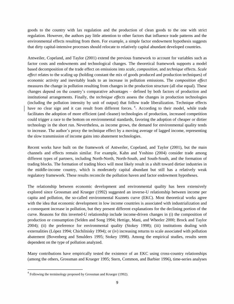
Figure 1 compares the emissions from clean and dirty industries in the period before and after DR-

CAFTA assuming no technique effect. All countries experience a significant increase in pollution

10 Most papers in the literature estimate a combination of scale and technique effects.

15

between the two periods. While for Costa Rica and El Salvador the additional emissions seem to come

mainly from dirty industries, both type of industries played a role in the expansion of emissions for

Nicaragua and Honduras. A more detailed analysis is necessary to assess the extent to which the variation

in pollution relates to changes in composition and to control for underlying trends in emissions.

Figure 1. Average pollution per year, before and after DR-CAFTA negotiation (pounds)

CRI

SVL

NIC

HND

Source: IPPS and authors calculations

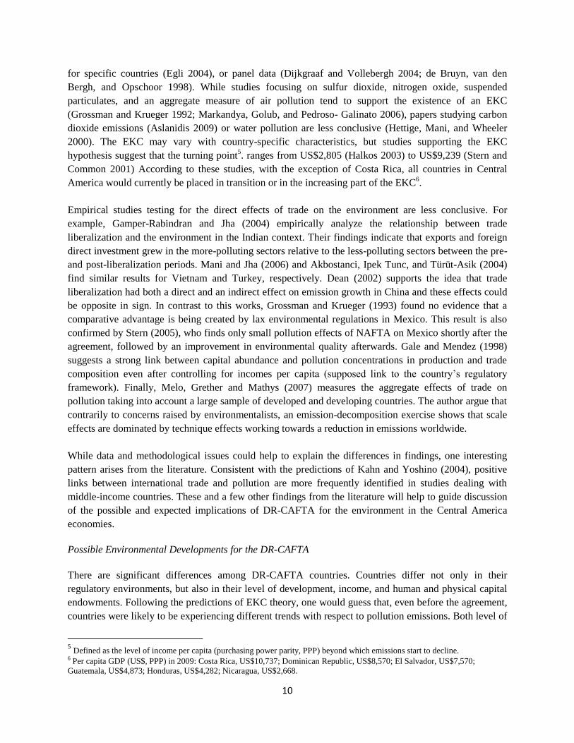
Figure 2 presents the results of the decomposition analysis under the baseline scenario for total

emissions11

(results for air, water and metal pollution can be found in the appendixAnnex 2). The first

striking fact of the analysis is the importance of scale effects. More than 90 percent of pollution variation

results from a scaling up of production. This is consistent across all countries in the sample. Composition

effects not only are smaller, but vary significantly across countries. For Costa Rica and El Salvador,

composition effects further expand pollution, while for the remaining countries (including the regional

11 The results for air, water, and metal pollution are available on request from the authors.

0

5000000

10000000

15000000

20000000

25000000

30000000

35000000

40000000

before after before after before after

air water total

clean dirty

0

10000000

20000000

30000000

40000000

50000000

60000000

70000000

80000000

before after before after before after

air water total

clean dirty

0

5000000

10000000

15000000

20000000

25000000

30000000

35000000

before after before after before after

air water total

clean dirty

0

2000000

4000000

6000000

8000000

10000000

12000000

14000000

16000000

18000000

before after before after before after

air water total

clean dirty

16

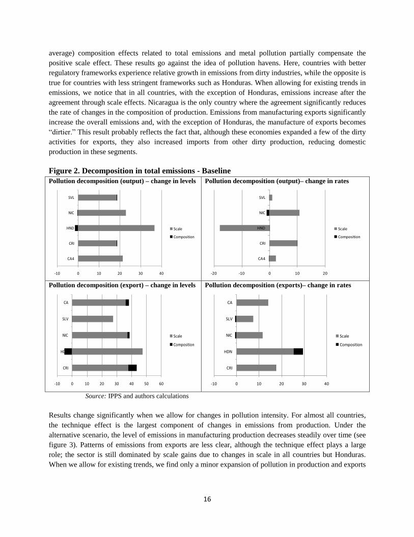
average) composition effects related to total emissions and metal pollution partially compensate the

positive scale effect. These results go against the idea of pollution havens. Here, countries with better

regulatory frameworks experience relative growth in emissions from dirty industries, while the opposite is

true for countries with less stringent frameworks such as Honduras. When allowing for existing trends in

emissions, we notice that in all countries, with the exception of Honduras, emissions increase after the

agreement through scale effects. Nicaragua is the only country where the agreement significantly reduces

the rate of changes in the composition of production. Emissions from manufacturing exports significantly

increase the overall emissions and, with the exception of Honduras, the manufacture of exports becomes

―dirtier.‖ This result probably reflects the fact that, although these economies expanded a few of the dirty

activities for exports, they also increased imports from other dirty production, reducing domestic

production in these segments.

Figure 2. Decomposition in total emissions - Baseline

Pollution decomposition (output) – change in levels

Pollution decomposition (output)– change in rates

Pollution decomposition (export) – change in levels

Pollution decomposition (exports)– change in rates

Source: IPPS and authors calculations

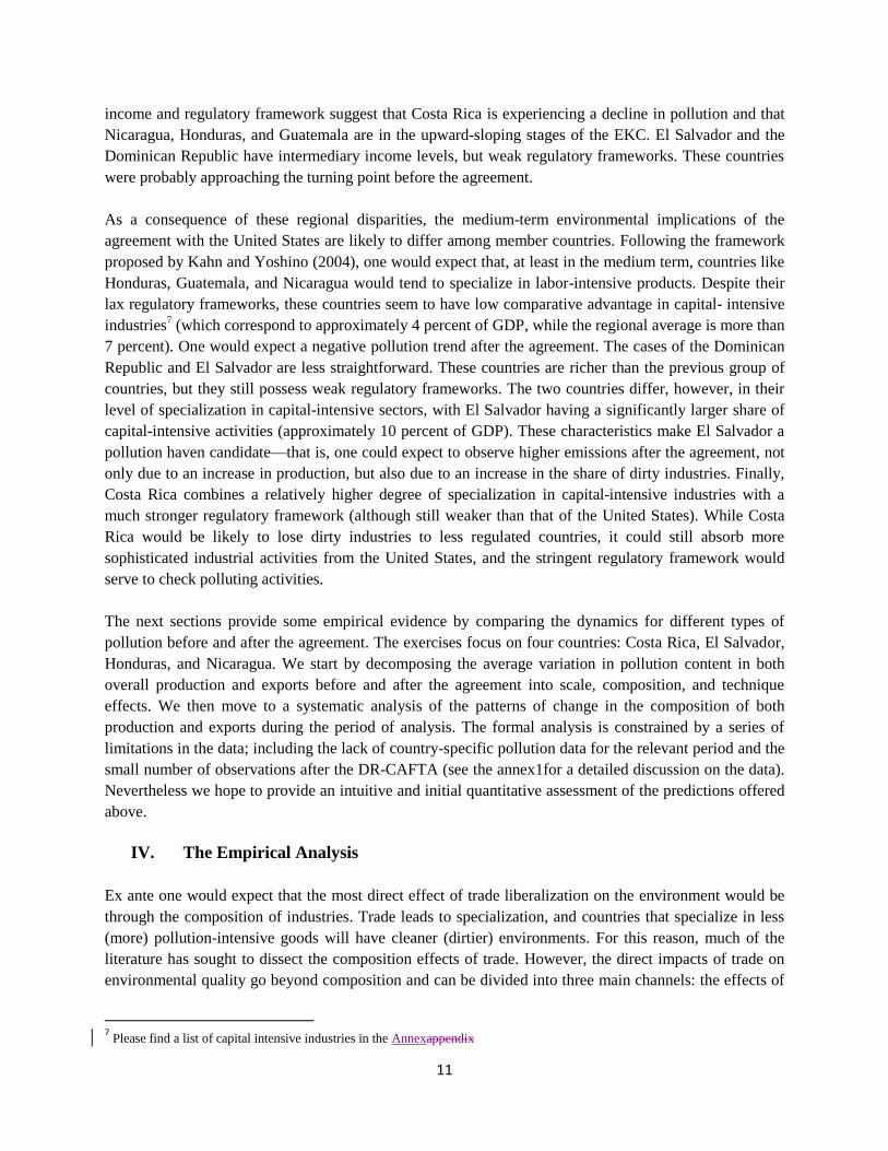
Results change significantly when we allow for changes in pollution intensity. For almost all countries,

the technique effect is the largest component of changes in emissions from production. Under the

alternative scenario, the level of emissions in manufacturing production decreases steadily over time (see

figure 3). Patterns of emissions from exports are less clear, although the technique effect plays a large

role; the sector is still dominated by scale gains due to changes in scale in all countries but Honduras.

When we allow for existing trends, we find only a minor expansion of pollution in production and exports

-10 0 10 20 30 40

CA4

CRI

HND

NIC

SVL

Scale

Composition

-20 -10 0 10 20

CA4

CRI

HND

NIC

SVL

Scale

Composition

-10 0 10 20 30 40 50 60

CRI

HDN

NIC

SLV

CA

Scale

Composition

-10 0 10 20 30 40

CRI

HDN

NIC

SLV

CA

Scale

Composition

17

after the agreement. The upward pressures related to scale gains are compensated by downward pressure

from the arrival and survival of cleaner technology.

Figure 3. Decomposition in total emissions – Alternative Scenario

Pollution decomposition (output) – change in levels

Pollution decomposition (output)– change in rates

Pollution decomposition (export) – change in levels

Pollution decomposition (exports)– change in rates

Source: IPPS and authors calculations

The decomposition analysis therefore suggests that the overall direction and size of changes in emissions

are largely dependent on assumptions about changes in technology. Nevertheless, some interesting

findings arise from the two extreme scenarios:

• Scale effects play a major role in explaining changes in emissions levels and trends after the

agreement.

• Composition effects are small and vary in direction across countries.

This effect is the focus of attention of the next exercise. While there seems to be no strong evidence

supporting the pollution haven hypothesis in Central America, the exercise shows significant gains from

the adoption of cleaner technologies.

Sector Composition Exercise

Table 1 presents the results of the regression analysis measuring changes in the composition of outputs

and exports, by sector, for the CA4. The results indicate a positive trend in the relative growth of dirty

industries before the beginning of DR-CAFTA negotiations. The trend disappears in the period after.

-20.00 -15.00 -10.00 -5.00 0.00 5.00 10.00 15.00

CRI

HDN

NIC

SLV

CA

Scale

Composition

Technique

-15.00 -10.00 -5.00 0.00 5.00 10.00 15.00

CRI

HDN

NIC

SLV

CA

Scale

Composition

Technique

-20.00 -10.00 0.00 10.00 20.00

CRI

HDN

NIC

SLV

CA

Scale

Composition

Technique

-30.00 -20.00 -10.00 0.00 10.00 20.00 30.00

CRI

HDN

NIC

SLV

CA

Scale

Composition

Technique

18

Results are only significant when total pollution is taken into account. Other types of pollutants do not

seem affected by the treat. Coefficients remain significant even after controlling for production factor

shares, which indicates that the dynamics of dirty industries go beyond traditional comparative

advantages. Results for exports follow a similar path. Dirty industry exports are expanding relative to

other industries before the agreement, but this trend disappears after the beginning of negotiations. The

main difference regarding the composition of exports is the fact that, after crossing the DR-CAFTA

dummy with the indicators of factor shares, trends in dirty industry exports become insignificant.

The results of the regression analysis for individual countries are presented in tTable 2. We focus here on

the analysis of total emissions. The results for other types of pollutants are presented in the

appendixAnnex 2. Results for Costa Rica indicate higher growth of output for dirty industries before the

agreement, but this trend is partially canceled after negotiations. As for Costa Rica’s exports, dirty

industries expand faster during the whole period. Regressions for El Salvador indicate no significant

effects of the agreement on the composition of output toward dirty industries. Growth seems to be driven

mainly by factor shares, with human capital-intensive industries expanding relatively faster. El Salvador’s

exports behave similarly to exports for the region, that is, the relatively higher growth of exports in dirty

industries slows significantly after the agreement takes place. In Nicaragua, the agreement seems to have

no impact on relatively pollution-intensive industries. During the sample period, growth favors labor-

intensive manufacturing activities. Finally, in Honduras, the agreement seems to have contributed to the

relative growth in the output of cleaner industries. This result remains significant even after controlling

for factor shares of production. Once more, results go against the common assumptions in the policy

debate.

Table 1: Regression Analysis: CA4

Dependent variable:

(1) (2) (3) (4) (5) (6) (7) (8) (1) (2) (3) (4) (5) (6) (7) (8)

Dirty Total 0.16 0.33** 0.35** 0.38** 0.81* 1.74** 1.67* 1.34

Dirty Air 0.11 0.28 0.30 0.30 0.79 17.04* 1.86 1.71

Dirty Water 0.07 0.17 0.17 0.17 0.42 9.91 0.85 0.46

Dirty Metal -0.08 -0.21 -0.24 -0.25 -0.75 -14.34** -2.11** -2.57**

After*Dirty Total -0.34* -0.35* -0.41* -1.75** -1.93* -1.30

After*Dirty Air -0.31 -0.33 -0.33 -17.30 -1.95 -1.67

After*Dirty Water -0.18 -0.19 -0.19 -10.71 -1.14 -0.39

After*Dirty Metal 0.24 0.25 0.26 13.00 1.45 2.31

Labor share -0.09 -0.19 -0.14 -0.24 -1.62 -2.72 -2.00 -3.23

Capital share 0.14 0.09 0.11 0.10 -1.23 -1.69 -0.88 -1.00

After*Labor 0.10 0.10 0.64 0.80

After*Capital 0.06 -0.01 -0.70 -1.41

N 168 168 168 168 168 168 169 170 168 168 168 168 147 147 147 147

Country fixed y y y y y y y y y y y y y y y y

*,** signinficant at 10% and 5% resp.

Note: the classification into dirty industries follows Mani et. al (1998)

annual output growth per 2-digit industry annual exports growth per 2-digit industry

19

Overall the quantitative exercises developed in this section find no evidence to support the formation of

pollution havens after DR-CAFTA negotiation. Annual levels of pollution seem to have increased after

the agreement, but changes were driven mainly by the increase in production. In none of the economies

analyzed do weak environmental regulatory frameworks seem to have played a major role in determining

comparative advantages. Changes in the composition of production are quite small and, in some cases

(like Honduras), favor cleaner sectors. Nevertheless, countries should continue pursuing their

environmental agenda and working to close regulatory gaps among member countries, as pollution

pressures tend to increase as economies grow. The environmental agenda should be combined with action

to improve and sustain competitiveness in the presence of higher regulatory costs.

VI. CONCLUSIONS

This paper analyzes the short-term and possible medium-term environmental impacts of the DR-CAFTA.

The paper started by reviewing DR-CAFTA’s environmental chapter and environmental regulatory

frameworks in member countries. It, then, revieweds the literature on Trade and the Environment and

discusseds the expected results of the agreement for the region. The paper proposes two empirical

exercises for assessing the changes in emissions following the DR-CAFTA negotiations. The first

exercise decomposes the pollution effect into scale, composition, and technique effects. The second

exercise focuses on changes in the composition of production and exports and assesses whether the

Table 2: Country Regressions

CRI HND

Dependent variable: Dependent variable:

(1) (2) (3) (4) (1) (2) (3) (4) (1) (2) (3) (4) (1) (2) (3) (4)

Dirty Total 0.64 0.34** 1.21** 1.23* 0.33** 0.51** 0.53** 0.62** Dirty Total 0.07 0.17* 0.08 1.08 -0.759 -1.005 -0.842 -1.40

After*Dirty Total -0.34* -1.13* -1.10 -0.31 -0.31 -0.47 After*Dirty Total -0.17* -0.17* -0.17* 0.492 0.49 1.60

Labor share -1.96 -1.72 -3.26* -3.17 Labor share -3.26 1.08 -8.41* -9.33*

Capital share -1.62 -1.02 -2.86* -2.96 Capital share -3.83* -4.04* -4.35 -4.27

After*Labor 0.33 -0.2 After*Labor -7.07** 7.8

After*Capital -0.22 After*Capital 0.17* -1.59

N 168 168 168 168 168 168 168 168 N 168 168 168 168 168 168 168 168

NIC SVL

Dependent variable: Dependent variable:

(1) (2) (3) (4) (1) (2) (3) (4) (1) (2) (3) (4) (1) (2) (3) (4)

Dirty Total -0.07 -0.09 -0.05 -0.01 3.14 6.36** 0.07 -0.05 Dirty Total -0.01 0.00 0.00 0.01 0.31 0.69** 0.69** 0.68*

After*Dirty Total 0.03 0.03 -0.04 -6.45* -0.48 -0.25 After*Dirty Total -0.02 -0.02 -0.06 -0.69* -0.69* -0.68

Labor share 0.62* 1.30** 5.81* 11.32** Labor share -16.27* -16.27* 3.08 3.08

Capital share 0.04 -0.03 -2.81** -2.83** Capital share -16.23* -16.32* 3.07 3.07

After*Labor -1.22 -11.02* After*Labor 0.02 1.00

After*Capital 0.13 0.05 After*Capital 0.04 -0.16

N 168 168 168 168 168 168 168 168 N 168 168 168 168 168 168 168 168

*,** signinficant at 10% and 5% resp.

Note: the classification into dirty industries follows

output growth per 2-digit ind exports growth per 2-digit ind output growth per 2-digit ind exports growth per 2-digit ind

output growth per 2-digit ind exports growth per 2-digit ind output growth per 2-digit ind exports growth per 2-digit ind

20

agreement favors the relative expansion of dirty industries. Two scenarios—no technical effect and a

positive technical effect—are considered for the analysis.

Results show that the environmental developments from DR-CAFTA vary significantly across member

countries. Most results are consistent with the findings in the literature. Scale effects are positive and

dominate the composition effects for all countries. Composition effects vary significantly across member

countries. While Costa Rica and El Salvador, countries with stronger environmental regulations,

experience a small but positive increase in pollution as a result of changes in the composition of

production, Nicaragua and Honduras (as well as the regional average) experience negative composition

effects. The results indicate that factors other than a lax regulatory framework play an important role in

determining the patterns of production and trade. Results change after allowing for adjustments in

pollution intensity. Under this alternative scenario, levels of emissions from production seem to have

decreased after the agreement. The share of pollution in exports continuously expands in the alternative

scenario as well.

The findings do not suggest the existence of pollution havens in Central America. Nonetheless, countries

should continue strengthening and homogenizing environmental rules in the region. The environmental

agenda should be combined with an effort to improve competitiveness that helps to sustain trade in the

medium term as regulatory costs rise.

References

Akbostanci, Elif, G. Ipek Tunc, and Serap Türüt-Asik. 2004. ―Pollution Haven Hypothesis and the Role

of Dirty Industries in Turkey’s Exports.‖ ERC Working Paper 0403, Middle East Technical University,

Economic Research Center, February.

Antweiler,Werner, Brian R. Copeland, and M. Scott Taylor. 2001. ―Is Free Trade Good for the

Environment?‖ American Economic Review 91 (4, September): 877–908.

Aslanidis, Nektarios. 2009.―Environmental Kuznets Curves for Carbon Emissions: A Critical Survey.‖

Working Paper 2009.75, Fondazione Eni Enrico Mattei, Milan.

Bovenberg, A. L., and Sjak Smulders. 1995. ―Environmental Quality and Pollution-Augmenting

Technological Change in a Two-Sector Endogenous Growth Model.‖ Journal of Public Economics 57 (3,

July): 369–91.

Brock,William A., and M. Scott Taylor. 2004. ―The Green Solow Model.‖ NBER Working Paper 10557,

National Bureau of Economic Research, Cambridge, MA.

Chichilnisky, Graciela. 1994. ―North-South Trade, Property Rights, and the Dynamics of Environmental

Resources.‖ MPRA Paper 8415, University Library of Munich, Germany.

21

Cole, Matthew A., and Anthony J. Rayner. 2000. ―The Uruguay Round and Air Pollution: Estimating the

Composition, Scale, and Technique Effects of Trade Liberalization.‖ Journal of International Trade and

Economic Development 9 (3, September): 339–54.

Copeland, Brian R., and M. Scott Taylor. 1994. ―North-South Trade and the Environment.‖ Quarterly

Journal of Economics 109 (3, August): 755–87.

———.2003. International Trade and Environment: Theory and Practice. Princeton, NJ: Princeton

University Press.

———. 2004. ―Trade, Growth, and the Environment.‖ Journal of Economic Literature 42 (1, March): 7–

71.

Dean, Judith M. 2002. ―Does Trade Liberalization Harm the Environment? A New Test.‖ Canadian

Journal of Economics 35 (4, November): 819–42.

de Bruyn, S. M., J. C. J. M. van den Bergh, and J. B. Opschoor. 1998. ―Economic Growth and Emissions:

Reconsidering the Empirical Basis of Environmental Kuznets Curves.‖ Ecological Economics 25 (2,

May): 161–75.

Di Maria, Corrado, and Sjak A. Smulders. 2004. ―Trade Pessimists vs. Technology Optimists: Induced

Technical Change and Pollution Havens.‖ Open Access Publication urn:hdl:10197/845, University

College Dublin.

Dijkgraaf, Elbert, and Herman Vollebergh. 2004. ―A Note on Testing for Environmental Kuznets Curves

with Panel Data.‖ Others 0409001, EconWPA.Washington University, St. Louis.

Egli, Hannes. 2004. ―The Environmental Kuznets Curve: Evidence from Time Series Data for Germany,‖

CER-ETH Economics Working Paper 03/28, Center of Economic Research, Swiss Federal Institute of

Technology (ETH), Zurich.

Esty, D., and M. Porter. 2005. ―National Environmental Performance: An Empirical Analysis of Policy

Results and Determinants.‖ Environment and Development Economics 10 (4): 391–434

Gale, Lewis R. and Mendez, Jose A., 1998. "The empirical relationship between trade, growth and the

environment," International Review of Economics & Finance, Elsevier, vol. 7(1), pages 53-61.

Gamper-Rabindran, Shanti, and Shreyasi Jha. 2004. ―Environmental Impact of India’s Trade

Liberalization.‖Working Paper, University of North Carolina at Chapel Hill, Department of Public Policy

.

Grether, Jean-Marie, Nicole A. Mathys, and Jaime de Melo. 2007. ―Trade, Technique, and Composition

Effects: What Is Behind the Fall in World-Wide SO2 Emissions 1990–2000?‖Working Paper 2007.93,

Fondazione Eni Enrico Mattei, Milan.

22

———. 2009. ―Scale, Technique, and Composition Effects in Manufacturing SO2 Emissions.‖

Environmental and Resource Economics 43 (2, June): 257–74.

Grossman, Gene, and Alan B. Krueger. 1992. ―Environmental Impacts of a North American Free Trade

Agreement.‖ CEPR Discussion Paper 644, Centre for Economic Policy Research, London.

———. 1995. ―Economic Growth and the Environment.‖ Quarterly Journal of Economics 110 (2, May):

353–77.

Halkos, George E. 2003. ―Environmental Kuznets Curve for Sulfur: Evidence Using GMM Estimation

and Random Coefficient Panel Data Models.‖Environment and Development Economics, Cambridge

University Press, vol. 8(04), pages 581-601, October

Hettige, Hemamala, Muthukumara Mani, and David Wheeler. 2000. ―Industrial Pollution in Economic

Development: Kuznets Revisited.‖ Journal of Development Economics 62 (2, August): 445–76.

Kahn, Matthew E., and Yutaka Yoshino. 2004. ―Testing for Pollution Havens Inside and Outside of

Regional Trading Blocs.‖ B. E. Journal of Economic Analysis and Policy 4 (2): art, 4.

López, Ramón. 1994. ―The Environment as a Factor of Production: The Effects of Economic Growth and

Trade Liberalization.‖ Journal of Environmental Economics and Management 27 (2, September): 163–84.

Mani, Muthukumara S. 1996. ―Environmental Tariffs on Polluting Imports: An Empirical Study.‖

Environmental and Resource Economics 7 (4): 391–411.

Mani, Muthukumara S., and Shreyasi Jha. 2006. ―Trade Liberalization and the Environment in Vietnam.‖

Policy Research Working Paper 3879,World Bank, April.

Mani, Muthukumara, and David Wheeler. 1998. ―In Search of Pollution Havens? Dirty Industry in the

World Economy, 1960–1999.‖ Journal of Environment and Development 7 (3, September): 215–47.

Markandya,Anil,Alexander Golub, and Suzette Pedroso-Galinato. 2006.―Empirical Analysis of National

Income and SO2 Emissions in Selected European Countries.‖ Environmental and Resource Economics 35

(3, November): 221–57.

Matthew E. Kahn & Yutaka Yoshino, (2004). "Testing for Pollution Havens Inside and Outside of

Regional Trading Blocs," The B.E. Journal of Economic Analysis & Policy, Berkeley Electronic Press,

vol. 0(2).

Péridy, Nicolas. 2006. ―Pollution Effects of Free Trade Areas: Simulations from a General Equilibrium

Model.‖ International Economic Journal 20 (1, March): 37–62.

Sarkar, S. 2009. ―A Study of the Environmental Issues Associated with the Dominican Republic–Central

American Free Trade Agreement (DR-CAFTA).‖ International Business and Economics Research

Journal 8 (1, January): 113–88.

23

Selden,T., and D. Song. 1994.―Environmental Quality and Development: Is There a Kuznets Curve for

Air Pollution Emissions?‖ Journal of Environmental Economics and Management 27 (2, September):

147–62.

Stern, David I., and Michael S. Common. 2001. ―Is There an Environmental Kuznets Curve for Sulfur?‖

Journal of Environmental Economics and Management 41 (2, March): 162–78.

Stern, David I., Michael S. Common, and Edward B. Barbier. 1996. ―Economic Growth and

Environmental Degradation: The Environmental Kuznets Curve and Sustainable Development.‖World

Development 24 (7, July): 1151–60.

Stokey, Nancy L. 1998. ―Are There Limits to Growth?‖ International Economic Review 39 (1, February):

1–31.

Tobey, James A. 1990. ―The Effects of Domestic Environmental Policies on Patterns of World Trade: An

Empirical Test.‖ Kyklos 43 (2): 191–209.

24

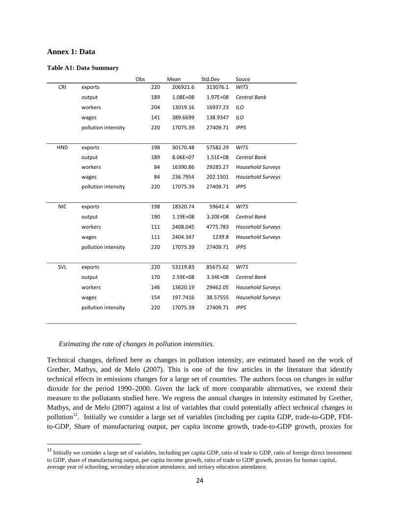
Annex 1: Data

Table A1: Data Summary

Obs Mean Std.Dev Souce

CRI exports 220 206921.6 313076.1 WITS

output 189 1.08E+08 1.97E+08 Central Bank

workers 204 13019.16 16937.23 ILO

wages 141 389.6699 138.9347 ILO

pollution intensity 220 17075.39 27409.71 IPPS

HND exports 198 30170.48 57582.29 WITS

output 189 8.06E+07 1.51E+08 Central Bank

workers 84 16390.86 29285.27 Household Surveys

wages 84 236.7954 202.1501 Household Surveys

pollution intensity 220 17075.39 27409.71 IPPS

NIC exports 198 18320.74 59641.4 WITS

output 190 1.19E+08 3.20E+08 Central Bank

workers 111 2408.045 4775.783 Household Surveys

wages 111 2404.347 1239.8 Household Surveys

pollution intensity 220 17075.39 27409.71 IPPS

SVL exports 220 53119.83 85675.62 WITS

output 170 2.59E+08 3.34E+08 Central Bank

workers 146 13620.19 29462.05 Household Surveys

wages 154 197.7416 38.57555 Household Surveys

pollution intensity 220 17075.39 27409.71 IPPS

Estimating the rate of changes in pollution intensities.

Technical changes, defined here as changes in pollution intensity, are estimated based on the work of

Grether, Mathys, and de Melo (2007). This is one of the few articles in the literature that identify

technical effects in emissions changes for a large set of countries. The authors focus on changes in sulfur

dioxide for the period 1990–2000. Given the lack of more comparable alternatives, we extend their

measure to the pollutants studied here. We regress the annual changes in intensity estimated by Grether,

Mathys, and de Melo (2007) against a list of variables that could potentially affect technical changes in

pollution12

. Initially we consider a large set of variables (including per capita GDP, trade-to-GDP, FDI-

to-GDP, Share of manufacturing output, per capita income growth, trade-to-GDP growth, proxies for

12 Initially we consider a large set of variables, including per capita GDP, ratio of trade to GDP, ratio of foreign direct investment

to GDP, share of manufacturing output, per capita income growth, ratio of trade to GDP growth, proxies for human capital,

average year of schooling, secondary education attendance, and tertiary education attendance.

25

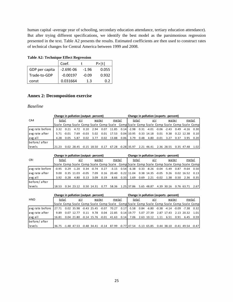
human capital -average year of schooling, secondary education attendance, tertiary education attendance).

But after trying different specifications, we identify the best model as the parsimonious regression

presented in the text. Table A2 presents the results. Estimated coefficients are then used to construct rates

of technical changes for Central America between 1999 and 2008.

Table A2: Technique Effect Regression

Coef. t P>|t|

GDP per capita -2.69E-06 -1.96 0.055

Trade-to-GDP -0.00197 -0.09 0.932

const 0.031664 1.3 0.2

Annex 2: Decomposition exercise

Baseline

Change in pollution (output- percent) Change in pollution (exports -percent)

CA4

Scale Comp Scale Comp Scale Comp Scale Comp Scale Comp Scale Comp Scale Comp Scale Comp

avg rate before 3.32 0.21 4.72 0.10 2.94 0.07 11.85 0.14 -2.98 0.31 -4.01 -0.06 -2.43 0.49 -4.16 0.30

avg rate after 5.71 -0.01 7.69 -0.03 5.02 0.01 17.53 0.04 10.95 0.33 14.18 0.01 9.38 0.22 12.38 0.10

avg a l l 4.28 0.05 5.87 0.02 3.77 0.02 13.88 0.06 3.79 0.48 4.80 -0.01 3.27 0.37 3.95 0.20

before/ after

levels 21.23 0.02 28.45 -0.15 18.50 0.17 67.28 -0.28 35.97 2.21 46.41 2.36 28.55 0.35 47.48 1.02

Change in pollution (output- percent) Change in pollution (exports -percent)

CRI

Scale Comp Scale Comp Scale Comp Scale Comp Scale Comp Scale Comp Scale Comp Scale Comp

avg rate before -0.95 0.29 -1.20 0.34 -0.74 0.27 -3.15 0.54 -6.38 0.33 -8.26 -0.04 -5.49 0.87 -9.64 0.50

avg rate after 9.00 0.35 11.03 -0.05 7.09 0.16 20.40 0.22 11.04 0.38 14.35 -0.05 9.26 0.02 16.52 0.13

avg a l l 3.92 0.28 4.80 0.13 3.09 0.19 8.66 0.33 1.69 0.69 2.21 -0.02 1.38 0.50 2.36 0.35

before/ after

levels 18.53 0.34 23.12 0.50 14.31 0.77 58.36 1.25 37.86 5.65 48.87 4.39 30.16 0.76 63.71 2.67

Change in pollution (output- percent) Change in pollution (exports -percent)

HND

Scale Comp Scale Comp Scale Comp Scale Comp Scale Comp Scale Comp Scale Comp Scale Comp

avg rate before 27.71 0.02 35.98 -0.43 25.45 -0.07 70.27 0.17 -5.58 0.84 -6.80 -0.38 -4.14 -0.09 -7.38 0.32

avg rate after 9.89 0.07 12.77 0.11 9.78 0.04 22.85 0.14 19.77 5.07 27.39 2.87 17.43 2.13 20.32 1.01

avg a l l 16.81 0.04 21.80 -0.14 15.76 -0.01 41.63 0.14 7.06 2.63 10.12 1.11 6.51 0.91 6.45 0.59

before/ after

levels 36.75 -1.48 47.53 -0.48 34.41 -0.14 87.99 -0.77 47.54 -5.13 65.85 0.44 38.10 -0.41 49.54 -0.47

water metal

total a i r water metal

total a i r water metal

total a i r

total a i r water metal

total a i r water metal

total a i r water metal

26

Alternative Scenario

Change in pollution (output- percent) Change in pollution (exports -percent)

NIC

Scale Comp Scale Comp Scale Comp Scale Comp Scale Comp Scale Comp Scale Comp Scale Comp

avg rate before -2.30 0.53 -3.89 0.22 -2.43 0.07 -14.11 0.16 6.89 0.07 12.13 -0.02 7.32 1.18 3.76 0.10

avg rate after 8.47 -0.47 14.60 -0.44 9.29 -0.26 55.64 -0.81 18.60 -0.57 33.89 -0.28 18.47 -0.10 11.25 -0.09

avg a l l 3.22 -0.05 5.55 -0.12 3.52 -0.10 21.21 -0.36 12.95 -0.22 23.29 -0.14 13.01 0.48 7.90 0.00

before/ after

levels 22.97 -0.37 39.50 -1.41 24.00 -0.59 140.54 -6.31 37.13 1.46 63.97 0.81 37.40 0.68 26.22 0.35

Change in pollution (output- percent) Change in pollution (exports -percent)

SVL

Scale Comp Scale Comp Scale Comp Scale Comp Scale Comp Scale Comp Scale Comp Scale Comp

avg rate before 2.46 0.07 3.09 0.05 2.10 -0.03 7.08 -0.09 2.41 0.07 2.67 0.03 1.72 0.08 2.93 0.05

avg rate after 3.48 0.07 4.38 0.08 2.90 0.06 10.64 0.11 9.84 -0.46 11.38 -0.34 8.02 0.56 9.78 0.00

avg a l l 2.83 0.02 3.56 0.04 2.38 -0.01 8.42 -0.02 6.43 -0.20 7.37 -0.15 5.07 0.26 6.70 0.00

before/ after

levels 18.46 0.34 23.17 -0.01 15.72 0.15 51.42 0.34 27.54 -0.28 31.13 -0.14 20.23 -0.07 32.35 -0.11

total a i r water metal

total a i r water metal total a i r water metal

total a i r water metal

Change in pollution (output- percent) Change in pollution (export - percent)

CA4

Scale Comp Tec Scale Comp Tec Scale Comp Tec Scale Comp Tec Scale Comp Tec Scale Comp Tec Scale Comp Tec Scale Comp Tec

avg before 0.53 0.01 -0.36 5.26 0.02 -6.49 3.21 0.13 -3.08 13.70 0.13 -13.11 4.92 0.25 -6.32 -3.11 -0.05 5.29 -1.87 0.41 0.25 -3.21 0.24 1.75

avg after 0.80 0.00 -0.06 7.69 -0.02 -5.88 5.02 0.01 -4.35 17.48 -0.01 -17.04 8.47 0.07 -7.29 11.51 -0.08 -11.01 7.64 0.19 -8.37 9.68 0.04 -10.53

avg all 0.63 0.00 -0.17 6.11 0.00 -5.43 3.89 0.05 -3.49 14.68 0.03 -14.06 6.36 0.29 -6.11 4.06 -0.05 -4.57 2.78 0.31 -3.94 3.22 0.14 -4.26

before/after 8.05 0.04 -12.77 10.78 -0.07 -15.41 6.99 0.05 -11.79 25.95 -0.14 -30.47 12.22 0.75 -17.32 15.51 0.71 -20.64 9.65 0.11 -14.27 15.81 0.32 -19.89

Change in pollution (output- percent) Change in pollution (export - percent)

CRI

Scale Comp Tec Scale Comp Tec Scale Comp Tec Scale Comp Tec Scale Comp Tec Scale Comp Tec Scale Comp Tec Scale Comp Tec

avg before -0.95 0.59 0.19 -1.20 0.11 0.87 -0.74 0.32 0.19 -3.15 0.46 2.84 -6.37 3.60 3.36 -8.37 1.93 6.96 -5.53 0.59 5.74 -9.62 1.26 8.56

avg after 9.00 0.32 -8.68 11.04 -0.05 -10.29 7.09 0.16 -6.60 20.36 0.08 -19.25 11.05 0.08 -9.92 14.31 0.12 -13.30 9.26 0.06 -7.99 16.50 0.11 -15.03

avg all 3.92 0.40 -4.09 4.80 0.02 -4.58 3.09 0.21 -3.09 8.64 0.24 -8.16 1.70 1.68 -2.47 2.15 0.93 -2.21 1.36 0.42 -0.74 2.36 0.75 -2.13

before/after 5.85 0.11 -11.55 7.27 0.16 -12.99 4.52 0.24 -10.44 18.64 0.40 -23.01 12.27 1.84 -18.41 15.91 1.43 -21.71 9.87 0.25 -14.51 20.33 0.85 -25.01

Change in pollution (output- percent) Change in pollution (export - percent)

HND

Scale Comp Tec Scale Comp Tec Scale Comp Tec Scale Comp Tec Scale Comp Tec Scale Comp Tec Scale Comp Tec Scale Comp Tec

avg before 2.34 -0.92 -1.66 3.01 -0.31 -2.99 2.19 0.11 -2.65 5.67 -0.32 -5.24 -5.57 -1.06 5.98 -6.82 -0.39 6.67 -4.15 0.15 3.40 -7.38 0.16 7.13

avg after 9.91 0.31 -9.29 12.76 0.05 -11.97 9.78 0.12 -8.80 22.86 0.04 -22.20 16.17 1.76 -18.58 22.43 1.44 -24.74 14.26 0.96 -15.62 15.84 -0.83 -16.77

avg all 5.95 -0.19 -5.36 7.66 -0.09 -7.20 5.82 0.10 -5.57 13.82 -0.10 -13.28 5.46 0.31 -6.15 7.90 0.47 -8.79 5.09 0.49 -5.81 4.46 -0.30 -4.87

before/after 8.01 -0.32 -14.31 10.35 -0.10 -16.86 7.45 -0.03 -14.23 19.39 -0.17 -25.67 9.43 -1.02 -15.77 13.08 0.09 -20.48 7.56 -0.08 -14.95 9.99 -0.09 -17.17

Change in pollution (output- percent) Change in pollution (export - percent)

NIC

Scale Comp Tec Scale Comp Tec Scale Comp Tec Scale Comp Tec Scale Comp Tec Scale Comp Tec Scale Comp Tec Scale Comp Tec

avg before -2.30 -0.16 2.25 -3.89 0.35 3.37 -2.43 0.19 2.23 -14.11 0.35 13.81 6.94 0.71 -6.54 12.24 1.50 -12.60 7.34 0.67 -6.63 3.75 0.28 -3.00

avg after 8.47 -0.57 -6.69 14.56 -0.27 -13.04 9.31 -0.28 -7.95 55.59 -0.81 -53.71 18.57 0.11 -17.00 33.86 0.11 -32.24 18.60 -0.65 -15.74 11.23 0.01 -10.33

avg all 3.21 -0.34 -2.36 5.53 0.01 -5.02 3.54 -0.09 -2.94 21.19 -0.36 -20.35 12.96 0.36 -11.85 23.33 0.71 -22.54 13.07 0.01 -11.26 7.89 0.13 -6.85

before/after 9.83 -0.16 -13.66 16.98 -0.61 -20.37 10.34 -0.26 -14.30 60.68 -2.71 -62.30 16.45 0.65 -20.61 28.36 0.36 -32.43 16.58 0.30 -19.96 11.63 0.15 -15.48

Change in pollution (output- percent) Change in pollution (export - percent)

SVL

Scale Comp Tec Scale Comp Tec Scale Comp Tec Scale Comp Tec Scale Comp Tec Scale Comp Tec Scale Comp Tec Scale Comp Tec

avg before 2.46 -0.11 -2.17 3.09 -0.08 -2.83 2.10 -0.01 -1.91 7.09 0.01 -6.57 2.41 0.07 -2.38 2.67 0.03 -2.66 1.73 0.08 -1.84 2.93 0.08 -2.42

avg after 3.48 0.10 -3.11 4.37 0.06 -3.95 2.91 0.05 -2.45 10.64 0.10 -10.86 9.84 0.80 -9.06 11.36 0.73 -10.69 8.00 0.14 -6.40 9.76 0.01 -8.15

avg all 2.83 -0.01 -2.49 3.56 -0.01 -3.21 2.38 0.00 -2.03 8.42 0.02 -8.07 6.42 0.35 -5.91 7.36 0.32 -6.88 5.06 0.08 -4.28 6.68 0.03 -5.51

before/after 8.38 0.15 -12.38 10.49 -0.01 -14.36 7.08 0.07 -10.90 23.48 0.15 -27.82 12.40 -0.12 -15.97 14.03 -0.06 -17.80 9.10 -0.03 -13.11 14.74 -0.05 -17.09

water metal

water metal

total air water metal

water metal

total air water metal

total air water metal

total air

total air

total air

total air water metal

total air water metal

total air water metal

total air water metal

27

Annex 3: Regression Analysis for Individual Countries

Regression Analysis: CRI

Dependent variable: annual output growth per 2-digit industry Dependent variable: annual exports growth per 2-digit industry

(1) (2) (3) (4) (5) (6) (7) (8) (1) (2) (3) (4) (5) (6) (7) (8)

Dirty Total 0.64 0.34** 1.21** 1.25* 0.33** 0.51** 0.53** 0.62**

Dirty Air 0.58 1.18 1.17 1.15 0.39** 0.50* 0.50* 0.51*

Dirty Water 0.34 0.66 0.64 0.58 0.13 0.26 0.27 0.30

Dirty Metal -0.49 -0.95* -0.96 -1.03 -0.38** -0.52** -0.52** -0.48*

After*Dirty Total -0.34* -1.13* -1.20 -0.31 -0.31 -0.47

After*Dirty Air -1.19 -1.20 -1.16 -0.21 -0.21 -0.23

After*Dirty Water -0.63 -0.64 -0.52 -0.24 -0.24 -0.30

After*Dirty Metal 0.92 0.93 1.06 0.25 0.25 0.18

Labor share -1.96 -1.56 -2.11 -1.72 -3.26* -2.88* -3.17 -2.80

Capital share -1.62 -1.14 -1.66 -1.02 -2.86* -2.41 -2.96 -2.47

After*Labor 0.31 0.33 -0.2 -0.16

After*Capital 0.07 -0.22 0.2 0.12

N 168 168 168 168 168 168 168 168 168 168 168 168 168 168 168 168

Regression Analysis: HND

Dependent variable: annual output growth per 2-digit industry Dependent variable: annual exports growth per 2-digit industry

(1) (2) (3) (4) (5) (6) (7) (8) (1) (2) (3) (4) (5) (6) (7) (8)

Dirty Total 0.07 0.17* 0.08 0.02 -0.76 -1.00 -0.84 -1.40

Dirty Air -0.06 -0.10 -0.08 -0.05 -0.03 -0.08 -0.11 -0.34

Dirty Water -0.01 -0.02 -0.08 -0.14 -0.51 -0.73 -0.69 -1.19

Dirty Metal 0.11* 0.19** 0.11 0.04 -1.42 -1.49 -1.65 -2.27*

After*Dirty Total -0.17* -0.17* -0.07 0.49 0.49 1.60

After*Dirty Air 0.05 0.05 0.01 0.09 0.09 0.55

After*Dirty Water 0.01 0.01 0.11 0.45 0.45 1.45

After*Dirty Metal -0.14* -0.14 -0.02 0.15 0.15 1.39

Labor share -3.26 -3.33 0.72 1.08 -8.41* -10.60** -9.33* -10.81**

Capital share -3.83* -3.93* -3.96* -4.04* -4.35 -5.74* -4.27 -5.67*

After*Labor -6.37** -7.07** 7.79 3.40

After*Capital 0.21** 0.17* -1.59 -2.14*

N 168 168 168 168 168 168 168 168 168 168 168 168 168 168 168 168

Regression Analysis: NIC

Dependent variable: annual output growth per 2-digit industry Dependent variable: annual exports growth per 2-digit industry

(1) (2) (3) (4) (5) (6) (7) (8) (1) (2) (3) (4) (5) (6) (7) (8)

Dirty Total -0.07 -0.09 -0.05 -0.01 3.14 6.36** 0.07 -0.05

Dirty Air -0.06 -0.10 -0.09 -0.08 2.97 6.09 -0.24 -0.26

Dirty Water -0.04 -0.05 -0.02 0.01 1.66 3.62 0.01 -0.03

Dirty Metal 0.04 0.03 0.06 0.09 -2.67 -4.96* 0.00 -0.14

After*Dirty Total 0.03 0.03 -0.04 -6.45* -0.48 -0.25

After*Dirty Air 0.07 0.07 0.05 -6.24 -0.19 -0.15

After*Dirty Water 0.01 0.01 -0.05 -3.93 -0.04 0.04

After*Dirty Metal 0.01 0.01 -0.04 4.57 -0.25 0.03

Labor share 0.62* 0.68 1.37** 5.81* 5.20* 11.32** 10.61**

Capital share 0.04 0.05 -0.02 -2.81** -2.85** -2.83** -2.85**

After*Labor -1.25 -11.02* -10.81*

After*Capital 0.14 0.05 -0.01

N 168 168 168 168 168 168 168 168 168 168 168 168 168 168 168 168

Regression Analysis: SVL

Dependent variable: annual output growth per 2-digit industry Dependent variable: annual exports growth per 2-digit industry

(1) (2) (3) (4) (5) (6) (7) (8) (1) (2) (3) (4) (5) (6) (7) (8)

Dirty Total -0.01 0.00 0.00 0.0176 0.31 0.69** 0.69** 0.68*

Dirty Air -0.01 0.00 -0.01 0.00 0.30 0.68* 0.75 0.73

Dirty Water -0.01 0.00 0.00 0.03 0.16 0.40 0.36 0.30

Dirty Metal -0.02 -0.02 -0.02 0.00 -0.28 -0.56* -0.69* -0.76*

After*Dirty Total -0.02 -0.02 -0.06 -0.69* -0.69* -0.68

After*Dirty Air -0.01 -0.01 -0.03 -0.69 -0.75 -0.71

After*Dirty Water -0.03 -0.03 -0.07 -0.43 -0.43 -0.32

After*Dirty Metal 0.00 0.00 -0.04 0.52 0.63 0.75

Labor share -16.27* -16.65* -16.27* -16.62* 3.08 3.08 3.08 3.08

Capital share -16.23* -16.20* -16.32* -16.25* 3.07 3.07 3.07 3.09

After*Labor 0.02 -0.05 1.00 5.8

After*Capital 0.04 0.08 -0.16 -2.0

N 168 168 168 168 168 168 168 168 168 168 168 168 168 168 168 168

*,** signinficant at 10% and 5% resp.

Note: the classification into dirty industries follows

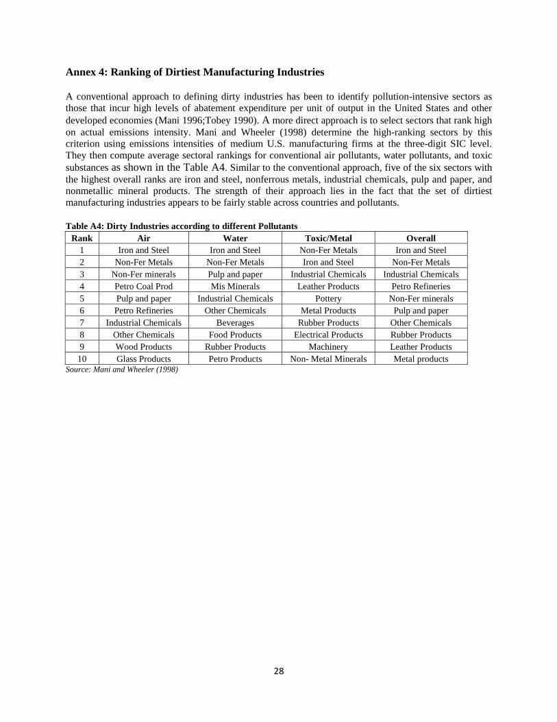
28

Annex 4: Ranking of Dirtiest Manufacturing Industries

A conventional approach to defining dirty industries has been to identify pollution-intensive sectors as

those that incur high levels of abatement expenditure per unit of output in the United States and other

developed economies (Mani 1996;Tobey 1990). A more direct approach is to select sectors that rank high

on actual emissions intensity. Mani and Wheeler (1998) determine the high-ranking sectors by this

criterion using emissions intensities of medium U.S. manufacturing firms at the three-digit SIC level.

They then compute average sectoral rankings for conventional air pollutants, water pollutants, and toxic

substances as shown in the Table A4. Similar to the conventional approach, five of the six sectors with

the highest overall ranks are iron and steel, nonferrous metals, industrial chemicals, pulp and paper, and

nonmetallic mineral products. The strength of their approach lies in the fact that the set of dirtiest

manufacturing industries appears to be fairly stable across countries and pollutants.

Table A4: Dirty Industries according to different Pollutants

Rank Air Water Toxic/Metal Overall

1 Iron and Steel Iron and Steel Non-Fer Metals Iron and Steel

2 Non-Fer Metals Non-Fer Metals Iron and Steel Non-Fer Metals

3 Non-Fer minerals Pulp and paper Industrial Chemicals Industrial Chemicals

4 Petro Coal Prod Mis Minerals Leather Products Petro Refineries

5 Pulp and paper Industrial Chemicals Pottery Non-Fer minerals

6 Petro Refineries Other Chemicals Metal Products Pulp and paper

7 Industrial Chemicals Beverages Rubber Products Other Chemicals

8 Other Chemicals Food Products Electrical Products Rubber Products

9 Wood Products Rubber Products Machinery Leather Products

10 Glass Products Petro Products Non- Metal Minerals Metal products Source: Mani and Wheeler (1998)