draft report on eo datasets - earth2observe.euearth2observe.eu/files/public...

This project has received funding from the European Union’s Seventh Programme for research, technological development and demonstration under grant agreement No. 603608

DG Research –FP7-ENV-2013-two-stage

Global Earth Observation for integrated water resource assessment

Draft Report on EO Datasets

Deliverable No: D.3.2 – Draft Report on EO Datasets Ref.: WP3 - Task 1

Date: November 2015

WP3 - Task 1 – D.3.2 Draft Report on EO Datasets

Deliverable Title D.3.2 – Draft Report on EO Datasets Filename E2O_D3.2_Draft_Report_EO_Datasets_v05.docx Authors Vincenzo Levizzani (CNR-ISAC)

Contributors Filipe Aires (Estellus)

Emmanouil N. Anagnostou (KKT ITC) Nikolaos Bartsotas (KKT ITC) Lukas Brodsky (GISAT) Elsa Cattani (CNR-ISAC) Daniel Chung (TU Wien) Chantal Claud (CNRS) Richard de Jeu (VU Amsterdam and Deltares) Geoffroy Detry (I-MAGE) Wouter A. Dorigo (TU Wien) Mike Grant (PML) Steve Groom (PML) Marketa Jindrova (GISAT) Lubos Kucera (GISAT) Sante Laviola (CNR-ISAC) Michel Lambotte (I-MAGE) Anna Cinzia Marra (CNR-ISAC) Gian Paolo Marra (CNR-ISAC) Frank S. Marzano (Univ. Roma La Sapienza) Inge Melotte (I-MAGE) Thomas Melzer (TU Wien) Gonzalo Miguez-Macho (Univ. Santiago de Compostela) Mario Montopoli (Univ. Roma La Sapienza) Saverio Mori (Univ. Roma La Sapienza) Efthymios Nikolopoulos (KKT ITC) Giulia Panegrossi (CNR-ISAC) Cathrine Prigent (Estellus) Jean-François Rysman (CNRS) Jaap Schellekens (Deltares) Stefan Simis (PML) Philip J. Ward (VU Amsterdam) Claudine Wenhaji Ndomeni (CNR-ISAC) Rogier Westerhoff (Deltares) Hessel Winsemius (Deltares)

Date 19/11/2015

Prepared under contract from the European Commission Grant Agreement No. 603608 Directorate-General for Research & Innovation (DG Research), Collaborative project, FP7-ENV-2013-two-stage Start of the project: 01/01/2014 Duration: 48 months Project coordinator: Stichting Deltares, NL


Dissemination level

X PU Public

PP Restricted to other programme participants (including the Commission Services)

RE Restricted to a group specified by the consortium (including the Commission Services)

CO Confidential, only for members of the consortium (including the Commission Services)

Deliverable status version control

Version Date Author

0.1 02/11/2015 Vincenzo Levizzani (CNR-ISAC)



0.4 20/11/2015 Frederiek Sperna Weiland (Deltares)



Table of Contents

1 Executive Summary ................................................................................................................................ 4

2 Introduction.............................................................................................................................................. 5

3 Precipitation............................................................................................................................................. 6

3.1 CDRD and PNPR ......................................................................................................................... 6

3.2 183-WSL ...................................................................................................................................... 8

3.3 PREC_X-SAR .............................................................................................................................. 9

3.4 PRECIP/MR/DC ......................................................................................................................... 11

3.5 SM2RAIN_ASCAT ..................................................................................................................... 11

3.6 3B42 ........................................................................................................................................... 12

3.7 CMORPH ................................................................................................................................... 13

3.8 GSMaP_MVK ............................................................................................................................. 14

3.9 PERSIANN ................................................................................................................................. 15

3.10 TAMSAT .................................................................................................................................... 16

3.11 RFE ............................................................................................................................................ 17

4 Soil moisture.......................................................................................................................................... 19

4.1 ECV_SM (CCI) ........................................................................................................................... 19

5 Evaporation and evapotranspiration ...................................................................................................... 20

5.1 GLEAM ...................................................................................................................................... 20

5.2 MOD16 ....................................................................................................................................... 21

6 Surface water ........................................................................................................................................ 21

6.1 GIEMS ....................................................................................................................................... 21

6.2 Surface water ............................................................................................................................. 23

6.2.1 Envisat ASAR-GM climatology 23

6.2.2 Landsat based 30 meter surface water mapping 23

6.3 Lake water level ......................................................................................................................... 25

7 Snow ..................................................................................................................................................... 25

7.1 Snow cover ................................................................................................................................ 25

7.2 Snowfall ..................................................................................................................................... 26

8 Water quality ......................................................................................................................................... 27

9 Water table depth in-situ observations .................................................................................................. 27

10 References ............................................................................................................................................ 30

11 Glossary ................................................................................................................................................ 33


List of Figure

Figure 1 Examples of precipitation retrievals of the CDRD (left, SSMIS overpass, 20 Jan 2012) and of the PNPR (right, Metop-AAMSU/MHS overpass, 6 Jan 2012) algorithms. The square on the CDRD image is blown up in the bottom plate where a cyclone is detected both by the algorithm and by the TRMM Precipitation Radar. ................................... 7 Figure 2 Example of precipitation retrieval over Europe with the 183-WSL algorithm of CNR. The algorithm identifies liquid and solid precipitation, water vapour content and also snow cover at the ground. Modules are under development for snowfall and hailfall retrievals. ............................................................................................................................................................. 8 Figure 3 Top: schematic view of the model used to compute the normalized radar cross section (NRCS) from a horizontally variable two-layer precipitating cloud. Bottom: X-band NRCS (in decibels) as a function of cross-track scanning distance x, showing enhanced values on the left of the crossover point caused by scattering from the cloud top and attenuation from rain in the lower cloud on the right. The cloud top is at zt, and the freezing height is z0, whereas the cloud width is w. The viewing (incidence) angle with respect to nadir is θ, whereas the surface background NRCS is σ0. Δr indicates the width of the slant slice of atmosphere representing the SAR side-looking resolution volume (this slant slice always includes the ground-range surface pixel). [Marzano et al., 2015; courtesy of IEEE]................................................................................................................................ 10 Figure 4 4 November 2011. 1st row: estimated rain rate [mm h-1] by X-SAR (left) and WR (right). 2nd row: cumulated precipitation 1h [mm] from rain gauges and their position. Vertical profiles of X-SAR attenuation [dB](3rd row) and WR reflectivity [dBZ] (4th row) for the two cross-track sections indicated on top panel (abscissas indicate longitude [deg]). .................................................................................................................................................................. 10 Figure 5 15-16 October 2012. Brightness temperature from MSG-SEVIRI 10.8 μm channel is shown as grey shading and superimposed are the pixel classified as deep convection (green) and convective overshooting (red). [Rysman et al., 2015; courtesy of Wiley]................................................................................................................................................................... 11 Figure 6 Flow chart of the SM2RAIN rain retrieval algorithm. [Brocca et al., 2014; courtesy of Wiley]........................................................................................................................................... 12 Figure 7 Mean seasonal rainrate (mm day-1) averaged between 1998 and 2010: JJA (a) and DJF (b). [Liu, 2015; courtesy of Elsevier] ..................................................................................... 13 Figure 8 CMORPH-derived weekly rain rate for the week between 3 and 10 November 2015. .................................................................................................................................................................... 14 Figure 9 Rainfall global map from GSMaP_MVK at 0.1 × 0.1 deg resolution on 1 July 2005. ................................................................................................................................................................................ 15 Figure 10 3-hourly accumulated rainfall global map from PERSIANN on 18 November 2015. .................................................................................................................................................................... 16 Figure 11 TAMSAT daily rainfall estimates for 10 January 2013 (left) and 21 August 2013

(right). The development of the daily dataset provides valuable full spatial coverage historic

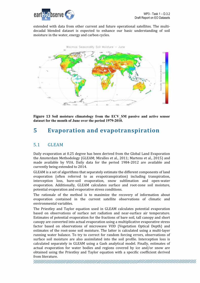
(1983 – present) and near real-time estimates on daily rainfall occurrence and amount. .......... 17 Figure 12 NOAA CPC RFE rainfall estimate over Africa (mm) for 16 November 2015. ....... 18 Figure 13 Soil moisture climatology from the ECV_SM passive and active sensor dataset for

the month of June over the period 1979-2010. ........................................................................................ 20 Figure 14 Schematics of the GLEAM model (left) and annual evaporation for the year 2000

(right). ................................................................................................................................................................... 21 Figure 15 Global satellite-derived inundation results over the 1993–2000 period with a 773 km2 spatial resolution (i.e., equal area grid of 0.25° × 0.25° at the equator). From bottom to top: (a) the annual maximum fractional inundation averaged over the 8 years, (b) the variability of the annual maximum fractional inundation (standard deviation of the maximum over the 8 years), (c) the mean annual number of inundated months, and (d) the most probable month of maximum inundation. [Prigent et al., 2007; courtesy of Wiley]................................................................................................................................................................... 22


Figure 16 Comparison of histogram built with the old code (left) and new code (right) over a 1 × 1 degree savannah area in West Africa. The new code reproduces the low incidence angles. ............................................................................................................................................. 23 Figure 17 Processing chain of Landsat and SRTM data into Surface Water Extent maps. ................................................................................................................................................................................ 24 Figure 18 Examples of snow cover mapping through MODIS (left) and MSG SEVIRI (right) optical sensors. ................................................................................................................................. 26 Figure 19 Snowstorm as observed by the N18-MHS on 30 March 2010, 0312 UTC. From the upper-left panel clockwise: the NIMROD radar precipitation rates, the NOAA SF, the 183-WSLSF, and the 183-SCM, which is the module of the 183-WSL method for computing the snow cover mask. ............................................................................................................. 26 Figure 20 Image of simulated depth to water table for Africa. [courtesy of Y. Fan, Rutgers Univ] ..................................................................................................................................................................... 28


1 Executive Summary

D3.2 “Draft Report on EO Datasets” as output of Task 3.1 is the first version of the comprehensive report on the description of remote sensing datasets available through the project data repository.

Data are available under the following main categories of observations of the Earth’s water cycle:

Evapotranspiration

Sub-surface water (Groundwater and Soil Moisture)

Inundation extent and dynamics (currently being uploaded)

Precipitation

State variables (Snow cover)

Surface water

Water quality

Datasets are meant to support the activities of the various work packages of the project, including WP4, WP5, WP6. They are also available to potential external end users since the project data portal is a one-stop repository, which can reveal very much instrumental for users who need various datasets at once for their model runs, data verification data validation, case studies on specific catchments or global studies.

The present version of the report is the first draft version and will be further refined in a successive version at month 34 of the project.


2 Introduction

Earth Observation (EO) datasets are available for relatively long time spans on the different aspects of the terrestrial water cycle. Several satellite missions were launched that observe precipitation, soil moisture, evaporation, evapotranspiration, inundated areas, sea and lake levels, surface water, snow cover and much more. While the Level 2 geophysical datasets created by these missions are relevant per se for the advancement of knowledge on the Earth water cycle, their usage has been all but massive to date. There is an overall tendency to limit the use of the datasets inside the scientific community that produces them and little effort has been dedicated to make other end user aware of their potential.

The eartH2Observe is gathering together a very diversified community of scientists and end users who are interested in the exploitation of Earth observation (EO) datasets for their everyday activities such as for example meteorologists, earth modellers, hydrologists, remote sensing specialists, water management experts. The idea is to come out with indications on the use of EO data, their potential and limitations, but from a hand-on point of view which stems from the actual use of the datasets.

The datasets are either 1) existing and well known datasets, or 2) new products being developed within the project. The latter are produced by new algorithms over limited regions and case studies to improve the resolution and the reliability of monitoring techniques of regional and global water resources. In some cases, the datasets represent unprecedented retrievals of geophysical variables.

The delivery of datasets is part of the mandate of WP3 “Earth Observations - Combining and improving EO processing techniques”, which focuses on the improvement of existing water cycle datasets and on the combination of multiple variables of the same indicator in a synergetic way.

Datasets are available on the following water cycle variables: evaporation, ground water, lake water level, precipitation (liquid and solid), snow cover, soil moisture, surface water, water quality (lakes).

The following satellite and sensors are used: GRACE, Cryosat-2, SMOS, ASCAT, EUMETSAT Polar System, Envisat ASAR Full Mission Archive, Envisat MERIS full resolution archive, ERS-1/2 Full Mission Archive, Sentinel-1 NRT data (when ready), COSMO-SkyMed X-SAR, TerraSAR-X and Tandem-X, Meteosat SEVIRI, MODIS Full Mission Archive, LandsatTM, GPM, TRMM, Megha-Tropiques, AMSU-A/B, AMSR-E, AMSR-2, SSMIS, ATMS, MetOp-B, AVHRR, Topex/Poseidon, Jason-1 and 2, VIIRS, AATSR and Sentinel-1, -2, -3 satellites (if available).

Non-European satellite products are included in the project especially in those cases where they improve the overall quality and accuracy of the end-products by contributing to the continuously evolving observing constellation.

D3.2, as output of Task 3.1, is the first draft version of the report describing the EO datasets of the project. A successive release on month 34 will include a refined version of the description also including advances made available during the project work.

In the following a description of the various datasets is provided divided in product categories.


3 Precipitation

Datasets on precipitation belong to two main categories: a) datasets made available by institutions not directly participating to the project, and b) datasets produced as a direct effort of the project. Moreover, they are either local or global datasets and their time span is of variable length depending on the availability of the satellite sensors on which they are based.

3.1 CDRD and PNPR

Datasets of new design were generated by exploiting new satellite algorithms based on passive MW developed at CNR, i.e. a) the Cloud Dynamics and Radiation Database (CDRD), based on a physically-based Bayesian approach applied to conically scanning radiometers (SSMIS) (Casella et al., 2013; Sanò et al., 2013), b) the Passive-microwave Neural-network Precipitation Retrieval (PNPR), designed to be applied to PMW cross-track scanning radiometers AMSU-A and MHS (or AMSU-B) and exploiting a neural network approach (Sanò et al., 2015).

The CDRD and PNPR algorithms, originally created for application over Europe and the Mediterranean basin, were recently modified and extended to Africa and Southern Atlantic for application to the MSG full disk area. This implied an upgrade of the synthetic a-priori (or training) cloud-radiation database built from cloud microphysical profiles coupled to a radiative transfer model and dynamic-thermodynamic-hydrologic (DTH) model-derived variables, taking into account African precipitating events, which is used in both algorithms, as a priori information in the CDRD and as training dataset in the PNPR. Applied to different weather conditions in Europe and Africa, the algorithms show good performance both in the identification of precipitation areas and in the retrieval of precipitation, particularly valuable over the extremely variable environmental and meteorological conditions of the region.

Some critical issues of the algorithms are considered. A new surface emissivity scheme in the generation of the synthetic cloud-radiation database has been introduced: FASTEM-4 (Liu et al., 2011) for ocean, and TELSEM (Aires et al., 2011) for land. This is mainly related to the ancillary data used in CDRD derived from the ECMWF analysis at 0.125° resolution. Moreover, a more sophisticated scheme for the treatment of the SSMIS pixels affected by land/sea transition has been introduced. A new detection scheme of precipitation over semi-arid land (for Africa) based on Casella et al. (2015) has been implemented in both algorithms.

After this analysis, a complete dataset of precipitation retrievals for the years 2011-2012-2013-2014 has been produced using both CDRD and PNPR algorithms. The CDRD algorithm receives as input the SSMIS brightness temperature TBs (SDR data) archived and publicly available from NOAA’s Comprehensive Large Array-Data Stewardship System (CLASS - http://www.class.ngdc.noaa.gov), while the PNPR algorithm receives as input the AMSU-A/MHS brightness temperature TBs (level 1B data converted to level 1C) archived and publicly available from NOAA’s Comprehensive Large Array-Data Stewardship System (CLASS - http://www.class.ngdc.noaa.gov).

Instantaneous precipitation rates are retrieved for a wide area covering Europe and Africa (60°S to 75°N latitude, 60°W to 60°E longitude), for each overpass of SSMIS and AMSU-A/MHS radiometers, respectively. The data are provided in netCDF 4 format. Each file contains data for one full orbit: rainfall rate (units mm h-1), phase, and quality index retrieved by CDRD and PNPR. Outside the area of interest (60°S to 75°N latitude,

http://www.class.ngdc.noaa.gov/


60°W to 60°E longitude), the values of rainfall rate, phase and quality index are set to missing value. The spatial resolution of the CDRD product is around 13.2 × 15.5 km2 while for PNPR it varies along the scan of the radiometer ranging from 16 × 16 km2 at nadir to 26 × 52 km2. The dataset format and product characteristics are fully described by a text description file provided with the data.

Figure 1 shows an example of retrievals using the two algorithms for two overpasses of the SSMIS and MHS over Europe and Africa.

Figure 1 Examples of precipitation retrievals of the CDRD (left, SSMIS overpass, 20 Jan 2012) and of the PNPR (right, Metop-AAMSU/MHS overpass, 6 Jan 2012) algorithms. The square on the CDRD image is blown up in the bottom plate where a cyclone is detected both by the algorithm and by the TRMM Precipitation Radar.

The dataset created in the framework of E2O has been used for a verification study carried out over the African region using the Tropical Rainfall Measuring Mission (TRMM) Precipitation Radar (PR) precipitation estimates (TRMM product 2A25) as ground-truth. The goal of the study was the verification of the ability of the two algorithms to retrieve precipitation over Africa and the Southern Atlantic, and to verify the consistency of the precipitation estimates and patterns derived from very different sensors, taking into account the different viewing geometry, spatial resolution, and channel frequency assortment of SSMIS and AMSU/MHS. All the analyses were performed using coincident observations (within a 15 min time

Rain

Rate

Rain

Rain

Rate

(mm

/h)


window) of the TRMM PR with observations from SSMIS and AMSU/MHS radiometers for the three year period 2011-2013. In this study, the co-located datasets of radiometers/PR observations were divided into three classes depending on the background surface – land, ocean, and coast - and the land class was subdivided into vegetated land and semi-arid land. The study has shown good abilities of the algorithms to screen out the not precipitating areas over the different types of background surface, good ability to retrieve light to moderate precipitation and heavy precipitation, while there is a tendency not to correctly identify very light precipitation. Moreover, while both CDRD and PNPR have shown good correlation with PR estimates, CDRD has quite similar performance for all the background surfaces, while PNPR shows a different behaviour between vegetated land and ocean.

3.2 183-WSL

The Water vapour Strong Lines at 183 GHz (183-WSL) algorithm conceived and designed at CNR exploits the three water vapour absorption frequencies around the band at 183.31 GHz of the AMSU-B/MHS sensors to retrieve precipitation.

Figure 2 Example of precipitation retrieval over Europe with the 183-WSL algorithm of CNR. The algorithm identifies liquid and solid precipitation, water vapour content and also snow cover at the ground. Modules are under development for snowfall and hailfall retrievals.

The 183-WSL method is still under development even though the algorithm performances in terms of precipitation detection skills and rain rate estimation accuracy are by now documented in the literature (Laviola et al., 2013). Recent improvements to the original retrieval scheme of the 183-WSL have been applied as result of research activity carried out at the NOAA’s Center for Satellite Applications and Research (STAR) and detailed in Laviola (2015). The investigation of various hailstorm events with the MicroWave Cloud Classification (MWCC) method highlights the high sensitivity of the method in identifying the large hail particles aloft clouds. The MWCC is a passive microwave method developed to characterize the cloud field in two main categories, stratiform and convective, by distinguishing the observed clouds


in three different evolution levels for each category. The classification is carried out by analysing the perturbation induced by clouds on the nominal signal (unperturbed) of the MHS water vapour channels. To approach the problem of hailstorm detection a rigorous selection of deep convection pixels as classified by the MWCC was matched with hailstorm events. The results of the study allowed us to develop a prototype method for hailstorm based on a model of growth improved with the dynamic carrying capacity, which calculates the probability occurrence of hail in the observed cloud. The prototype hail model is also now included in the 183-WSL computational scheme and it has been validated over the US by using the NOAA official hail reports as ground truth.

A method for detection of snowfall based on the frequency range 90 - 190 GHz of the Advanced Microwave Sounding Unit-B (AMSU-B) and Microwave Humidity Sounder (MHS) is now under improvement and testing as a module of the algorithm. The new algorithm is a prototype module of the 183-WSL retrieval scheme (Laviola and Levizzani, 2011) originally proposed in (Laviola et al., 2010). The previous studies have shown the skills of the 183-WSL algorithm to discern different types of precipitation via the identification of various hydrometeor phases as the method is highly sensitive both to liquid and solid hydrometeors (Laviola et al., 2013). Although the separation between different precipitating ice particles is difficult especially over frozen soils, the current version of the 183-WSL is improved with a prototype snowfall processor (183-WSLSF) working for land and open water. Recently, the 183-WSLSF performances have been compared with results of the NOAA SF method (Kongoli et al., 2015) showing high capabilities in detecting snowfall areas. The 183-WSLSF prototype from one hand reveals a systematic overestimation in the quantification of very light snowfall rates (< 0.5÷1.0 mm h-1) from the other it shows high sensitivity in reproducing the patterns of snow clouds as observed by radar (Laviola et al., 2015).

An example of retrieval is provided in Figure 2.

3.3 PREC_X-SAR

The group of the University of Roma “La Sapienza” (SUR) has devised a retrieval algorithm from synthetic aperture radar (SAR) observations from the TerraSAR-X (TSX) and COSMOSkyMed (CSK) sensors. Archives are available for the 2009-2013 period over the Mediterranean basin and other regions of interest of the project up to 2015.

Marzano et al. (2010) have demonstrated the capability of X-band SAR (X-SAR) sensors to detect rainfall over both sea and land, which can also be exploited to correct SAR imagery for rainfall attenuation effects. The overall scheme of the model is shown in Figure 3.

After the data collection and processing for a fist release, the refinement of a forward model of SAR response to improve X-SAR retrieval algorithms for detection and estimation of rainfall over land/sea is pursued. In particular, the SAR response model has been extended to polarimetric observations by including a full description of the copolar correlation coefficient and the differential phase. These variables can in principle help for the background discrimination and improve the rainfall retrieval algorithms. The background of the scene can include not only a land surface (bare soil, vegetation), but also a rough wind-driven surface and this situation makes the rain retrieval more challenging.

Figure 4 shows an example of rainfall retrieval on 4 November 2011.


Figure 3 Top: schematic view of the model used to compute the normalized radar cross section (NRCS) from a horizontally variable two-layer precipitating cloud. Bottom: X-band NRCS (in decibels) as a function of cross-track scanning distance x, showing enhanced values on the left of the crossover point caused by scattering from the cloud top and attenuation from rain in the lower cloud on the right. The cloud top is at zt, and the freezing height is z0, whereas the cloud width is w. The viewing (incidence) angle with respect to nadir is θ, whereas the surface background NRCS is σ0. Δr indicates the width of the slanted slice of atmosphere representing the SAR side-looking resolution volume (this slanted slice always includes the ground-range surface pixel). [Marzano et al., 2015; courtesy of IEEE]

Figure 4 4 November 2011. 1st row: estimated rain rate [mm h-1] by X-SAR (left) and WR (right). 2nd row: cumulated precipitation 1h [mm] from rain gauges and their position. Vertical profiles of X-SAR attenuation [dB](3rd row) and WR reflectivity [dBZ] (4th row) for the two cross-track sections indicated on top panel (abscissas indicate longitude [deg]).


3.4 PRECIP/MR/DC

CNRS makes use of the data provided by the Advanced Microwave Sounding Unit-B (AMSU-B) radiometer, replaced on recent platforms by the Microwave Humidity Sounder (MHS), which permit a concomitant observation of convection/precipitation occurrence over land and sea at a temporal resolution higher than that of meteorological analyses and with a fine-scale spatial resolution (roughly 20 km). Brightness temperatures measured since 1999 by channels of the AMSU-B and MHS sensors in the water vapour absorption line (183-191 GHz) indeed allow a screening of precipitation over sea, land and coastal regions. For each satellite, the dataset consists of twice-daily (a.m. and p.m.) and monthly maps of precipitation and convection occurrence on a global 0.2° lat × 0.2° lon grid for the Mediterranean area, i.e. 25 –60 N, 10 W–50 E. The period covered so far goes from 2000 to 2012, making use of NOAA-15 to -19 and Metop-A and B satellites. Precipitation and convection occurrences are available separately for the different sensors. Compared to a first version developed following Funatsu et al. (2009), some changes have been introduced, with in particular the withdrawal of a test which was supposed to discriminate precipitating snow from snow on the ground and which has been found too conservative. Efforts are still in progress to improve the database for such conditions.

Lately, special emphasis has been put on the HyMeX SOP1 period for which a vast amount of observations are available (September-October 2012). A new diagnostic has been developed, COV (Convective Overshooting), which discriminates among convective clouds those, which each the lower stratosphere (Figure 5; Rysman et al., 2015).

In parallel, the dataset is gradually extended to the tropical regions, and the consistency between the different radiometers/satellites investigated. The extension of the database to ATMS (Advanced Technology Microwave Sounder) aboard NPP satellites, which will replace MHS on some platforms, is also in progress.

Figure 5 15-16 October 2012. Brightness temperature from MSG-SEVIRI 10.8 μm channel is shown as grey shading and superimposed are the pixel classified as deep convection (green) and convective overshooting (red). [Rysman et al., 2015; courtesy of Wiley]

3.5 SM2RAIN_ASCAT

SM2RAIN is a novel “bottom-up” approach to rainfall estimation from space, which by doing “hydrology backward,” uses variations in soil moisture (SM) sensed by microwave satellite sensors to infer preceding rainfall amounts. It is developed by CNR and TU Wien in a joint effort.


The SM2RAIN algorithm is based on the inversion of the soil water balance equation for retrieving rainfall from SM data. The soil is assumed to work as a natural rain gauge for measuring the amount of rainfall fallen into the ground. Specifically, the soil water balance equation for a layer depth Z [L] can be described by the following expression:

Z ds(t) / dt = p(t) _- r(t) – e(t) – g(t)

where s(t) is the relative saturation of the soil or relative SM, t [T] is the time and p(t), r(t), e(t), and g(t) [L/T] are the precipitation, runoff, evapotranspiration, and drainage rate, respectively (Brocca et al. 2014). Whenever it rains, the evaporation rate can be safely assumed as negligible (e(t) = 0). Moreover, by assuming that all precipitation infiltrates into the soil, the runoff rate is zero (r(t) = 0). For the drainage rate, the following relation may be adopted, g(t) = as(t)b, where a [L/T] and b [_] are two parameters expressing the nonlinearity between drainage rate and soil saturation. The rearrangement of equation (1), with the described assumptions, yields to

p(t) ≅ Z ds(t)/dt + a s(t)b

This equation can be used for estimating the precipitation rate from the knowledge of relative SM, s(t), its fluctuations in time, ds(t)/dt, and three parameters (Z, a, and b) to be estimated through calibration. Even though the assumptions made for deriving equation (2) might introduce some errors, they allow obtaining a simple (but effective) method for the retrieval of rainfall from SM data (Brocca et al., 2013) that can be easily applied on a global scale.

The dataset is provided in kind to the project and makes use of the Advanced SCATterometer (ASCAT).

Figure 6 Flow chart of the SM2RAIN rain retrieval algorithm. [Brocca et al., 2014; courtesy of Wiley]

3.6 3B42

The purpose of the 3B42 algorithm is to produce Tropical Rainfall Measuring Mission (TRMM) merged high quality (HQ)/infrared (IR) precipitation and root-mean-square


(RMS) precipitation-error estimates. These gridded estimates are on a 3-hour temporal resolution and a 0.25-degree by 0.25-degree spatial resolution in a global belt extending from 50 degrees South to 50 degrees North latitude.

The 3B42 estimates are produced in four stages; (1) the microwave precipitation estimates are calibrated and combined, (2) infrared precipitation estimates are created using the calibrated microwave precipitation, (3) the microwave and IR estimates are combined, and (4) rescaling to monthly data is applied. Each precipitation field is best interpreted as the precipitation rate effective at the nominal observation time (Huffman et al. 2007).

The dataset in the project repository consists of 3-hourly rainfall estimates from v7 of the algorithm. For an overview of the differences between v6 and v7 of the algorithm see Liu (2015) (se also Figure 7).

Figure 7 Mean seasonal rainrate (mm day-1) averaged between 1998 and 2010: JJA (a) and DJF (b). [Liu, 2015; courtesy of Elsevier]

3.7 CMORPH

The Climate Prediction Center (CPC) MORPHing technique (CMORPH; Joyce et al., 2004) produces global precipitation analyses at very high spatial and temporal resolution. This technique uses precipitation estimates that have been derived from low orbiter satellite microwave observations exclusively, and whose features are transported via spatial propagation information entirely obtained from geostationary satellite IR data. Precipitation estimates derived from passive microwave sensors aboard the DMSP 13, 14 & 15 (SSM/I), the NOAA-15, 16, 17 & 18 (AMSU-B), and AMSR-E and TMI aboard NASA's Aqua and TRMM spacecraft, respectively. Note that


this technique is not a precipitation estimation algorithm, but a means by which estimates from existing microwave rainfall algorithms can be combined. Therefore, this method is extremely flexible such that any precipitation estimate from any microwave satellite source can be incorporated.

With regard to spatial resolution, although the precipitation estimates are available on a grid with a spacing of 8 km (at the equator), the resolution of the individual satellite-derived estimates is coarser than that - more on the order of 12 x 15 km2 or so. The finer "resolution" is obtained via interpolation.

In effect, IR data are used as a means to transport the microwave-derived precipitation features during periods when microwave data are not available at a location. Propagation vector matrices are produced by computing spatial lag correlations on successive images of geostationary satellite IR which are then used to propagate the microwave derived precipitation estimates. This process governs the movement of the precipitation features only. At a given location, the shape and intensity of the precipitation features in the intervening half hour periods between microwave scans are determined by performing a time-weighting interpolation between microwave-derived features that have been propagated forward in time from the previous microwave observation and those that have been propagated backward in time from the following microwave scan. We refer to this latter step as "morphing" of the features.

Figure 8 shows an example of weekly precipitation intensity derived from CMORPH.

Figure 8 CMORPH-derived weekly rain rate for the week between 3 and 10 November 2015.

3.8 GSMaP_MVK

The Global Satellite Mapping of Precipitation (GSMaP) MVK product produces global precipitation distribution with high temporal and spatial resolution. The technique uses the Kalman filter to compute the estimates of the current surface rain fall rates at each 0.1 degree pixel of the infrared brightness temperature by the GEO-IR satellites. The filter predict the precipitation rate from the microwave radiometer and its morphed product obtained in a similar way as the Joyce et al. (2004), and then refine the prediction based on the relationship between the IR brightness temperature and surface rainfall rate. In No.3 DVD product, the backward process is introduced to produce the global precipitation map as is the same in No.2. The rain rates from the passive microwave radiometers are generated by Aonashi and Liu (2000). See Ushio et al. (2009) for details.


Figure 9 Rainfall global map from GSMaP_MVK at 0.1 × 0.1 deg resolution on 1 July 2005.

3.9 PERSIANN

The Precipitation Estimation from Remotely Sensed Information using Artificial Neural Networks (PERSIANN; Hsu et al. 1997; Sorooshian et al., 2000) algorithm uses neural network function classification/approximation procedures to compute an estimate of rainfall rate at each 0.25° x 0.25° pixel of the IR brightness temperature image provided by geostationary satellites. An adaptive training feature facilitates updating of the network parameters whenever independent estimates of rainfall are available. The PERSIANN system was based on geostationary infrared imagery and later extended to include the use of both infrared and daytime visible imagery. The PERSIANN algorithm used here is based on the geostationary longwave infrared imagery to generate global rainfall. Rainfall product covers 50°S to 50°N globally.

The system uses grid IR images of global geosynchronous satellites (GOES-8, GOES-10, GMS-5, Metsat-6, and Metsat-7) provided by CPC, NOAA to generate 30-minute rain rates are aggregated to 6-hour accumulated rainfall. Model parameters are regularly updated using rainfall estimates from low-orbital satellites, including TRMM, NOAA-15, -16, -17, DMSP F13, F14, F15.

The processing steps are as follows

Global full resolution IR composites are downloaded from the NCEP Server on daily basis, these are 15 minute

1. TRMM level 2A (TRMM-2A25) microwave imager data are downloaded twice a day also with two days delay.

2. The NOAA Satellite Active Archive system is polled every 30 minutes to acquire the most recent microwave-based precipitation estimate from 6 additional microwave instruments on board NOAA K,L, and M (15,16 and 17, respectively) and DMSP 7,8 and 9. Because these data are available in real-near time, they are archived for use whenever the corresponding global IR composites become available.

3. Each day, CHRS’s the Global IR data is used to produce the intermediate 30 minutes 4 km precipitation product with the neural network model is trained using all microwave-based precipitation estimates available for the given day.


4. The intermediate product is then aggregated to 0.25° six hourly precipitation maps 3. And the product is released as provisional PERSIANN precipitation estimates. At the same time, 24 hr, 3, 5, 7, 10, 15, and 30 days total precipitation products are also created for distribution over the HyDIS-GWADI (Link) Server.

An example of 3-hourly accumulated rainfall from PERSIANN for 18 November 2015 is given in Figure 10.

Figure 10 3-hourly accumulated rainfall global map from PERSIANN on 18 November 2015.

3.10 TAMSAT

TAMSAT stands for Tropical Applications of Meteorology using SATellite data and ground-based observations, a dataset provided and maintained by the Dept. of Meteorology at the University of Reading.

The TAMSAT research group have provided 10-day (decade) rainfall estimates routinely since the late 1980s for Africa using Meteosat thermal infrared observations. Rainfall is estimated under the assumption that the length of time the cloud top temperature is below a predetermined threshold, known as the cold cloud duration (CCD), is linearly related to rainfall.

The TAMSAT rainfall estimation algorithm is locally calibrated using historic rain gauge records producing monthly and regional calibration parameters that are applied historically and in real-time to provide an internally consistent rainfall dataset, known as the TAMSAT African Rainfall Climatology and Time-series (TARCAT) (Maidment et al., 2014), which was recently extended over Africa in the context of a drought monitoring programme (Tarnavsky et al., 2014). This overcomes the need for near real-time rain gauge observations, which are typically sparse, unevenly distributed, and report sporadically. These estimates have been crucial, particularly in famine and drought early warning where reliable near real-time rainfall estimates providing full spatial coverage is essential. However, to meet the increasing demand for rainfall estimates at finer temporal scales, the TAMSAT Research Group has developed a simple approach designed to provide rainfall information at the daily time step (for example see Figure 11). Such information is vitally important for drought monitoring, such as capturing dry spells during the crop growing season, and can be most beneficial where very few or no rain gauge observations are available.

Operational TAMSAT products are:

daily and ten-daily (dekadal) cumulative rainfall estimates issued on the 1st, 11th and 21st of the month;

http://www.met.reading.ac.uk/~tamsat/data_use_policy/?data=rfe


monthly cumulative rainfall estimates issued on the first day of the following month;

seasonal cumulative rainfall estimates issued on 1st March, 1st June, 1st September and 1st December.

All the products are provided at 4 km resolution for the whole of Africa.

TAMSAT rainfall estimates are derived from Meteosat thermal infra-red (TIR) channels based on the recognition of convective storm clouds and calibration against ground-based rain gauge data.

Figure 11 TAMSAT daily rainfall estimates for 10 January 2013 (left) and 21 August

2013 (right). The development of the daily dataset provides valuable full spatial

coverage historic (1983 – present) and near real-time estimates on daily rainfall

occurrence and amount.

3.11 RFE

As of January 1, 2001, the CPC African Rainfall Estimates RFE version 2.0 (Xie and Arkin, 1996) has been implemented by NOAA's Climate Prediction Center. It replaces RFE 1.0, the previous rainfall estimation algorithm that was operational from 1995 through 2000. RFE 2.0 uses additional techniques to better estimate precipitation while continuing the use of cloud top temperature and station rainfall data that formed the basis of RFE 1.0. Meteosat 7 geostationary satellite infrared data is acquired in 30-minute intervals, and areas depicting cloud top temperatures of less than 235 K are used to estimate convective rainfall. WMO Global Telecommunication System (GTS) data taken from ~1000 stations provide accurate rainfall totals, and are assumed to be the true rainfall near each station. RFE 1.0 used an interpolation method to combine Meteosat and GTS data for daily precipitation estimates, and warm cloud information was included to obtain decadal estimates. The two new satellite rainfall estimation instruments that are incorporated into RFE 2.0 are the Special Sensor Microwave/Imager (SSM/I) on board Defense Meteorological Satellite Program satellites, and the Advanced Microwave Sounding Unit (AMSU). Both


estimates are acquired at 6-hour intervals and have a resolution of 0.25 degrees. RFE 2.0 obtains the final daily rainfall estimation using a two part merging process, then sums daily totals to produce dekadal estimates. All satellite data is first combined using a maximum likelihood estimation method, and then GTS station data is used to remove bias. Warm cloud precipitation estimates are not included in RFE 2.0.

Figure 12 NOAA CPC RFE rainfall estimate over Africa (mm) for 16 November

2015.


4 Soil moisture

4.1 ECV_SM (CCI)

Combining information derived from satellite-based passive and active microwave sensors has the potential to offer improved estimates of surface soil moisture at global scale. TU Wien has made available the soil moisture dataset from the ESA Climate Change Initiative (CCI)

The ESA CCI soil moisture group has developed and evaluated a methodology that takes advantage of the retrieval characteristics of passive (AMSR-E) and active (ASCAT) microwave satellite estimates to produce an improved soil moisture product (Liu et al., 2011). First, volumetric soil water content (m3 m−3) from AMSR-E and degree of saturation (%) from ASCAT are rescaled against a reference land surface model dataset using a cumulative distribution function matching approach. While this imposes any bias of the reference on the rescaled satellite products, it adjusts them to the same range and preserves the dynamics of original satellite-based products. Comparison with in situ measurements demonstrates that where the correlation coefficient between rescaled AMSR-E and ASCAT is greater than 0.65 ("transitional regions"), merging the different satellite products increases the number of observations while minimally changing the accuracy of soil moisture retrievals. These transitional regions also delineate the boundary between sparsely and moderately vegetated regions where rescaled AMSR-E and ASCAT, respectively, are used for the merged product. Therefore, the merged product carries the advantages of better spatial coverage overall and increased number of observations, particularly for the transitional regions. The combination method developed has the potential to be applied to existing microwave satellites as well as to new missions. Accordingly, a long-term global soil moisture dataset can be developed and extended, enhancing basic understanding of the role of soil moisture in the water, energy and carbon cycles.

Liu et al. (2012) have followed an active-passive microwave merging strategy:

1. Combine four passive microwave products from the VU University Amsterdam/NASA and two active microwave products from the Vienna University of Technology. First, passive microwave soil moisture retrievals from the Scanning Multichannel Microwave Radiometer (SMMR), the Special Sensor Microwave Imager (SSM/I), and the Tropical Rainfall Measuring Mission microwave imager (TMI) instruments were scaled to the climatology of the Advanced Microwave Scanning Radiometer — Earth Observing System (AMSR-E) derived product and then all four were combined into a single merged passive microwave product.

2. Combine two active microwave products from the ERS Scatterometer and from ASCAT into a merged active microwave product.

3. The two merged products were rescaled to a common globally available reference soil moisture dataset provided by a land surface model (GLDAS-1-Noah) and then blended into a single passive/active product. Blending of the active and passive datasets was based on their respective sensitivity to vegetation density.

While this three step approach imposes the absolute values of the land surface model dataset to the final product, it preserves the relative dynamics (e.g., seasonality and inter-annual variations) of the original satellite derived retrievals. More importantly, the long term changes evident in the original soil moisture products were also preserved. The method presented in this paper allows the long term product to be


extended with data from other current and future operational satellites. The multi-decadal blended dataset is expected to enhance our basic understanding of soil moisture in the water, energy and carbon cycles.

Figure 13 Soil moisture climatology from the ECV_SM passive and active sensor

dataset for the month of June over the period 1979-2010.

5 Evaporation and evapotranspiration

5.1 GLEAM

Daily evaporation at 0.25 degree has been derived from the Global Land Evaporation the Amsterdam Methodology (GLEAM; Miralles et al., 2011; Martens et al., 2015) and made available by VUA. Daily data for the period 1984-2012 are available and currently being extended to 2014.

GLEAM is a set of algorithms that separately estimate the different components of land evaporation (often referred to as evapotranspiration) including transpiration, interception loss, bare-soil evaporation, snow sublimation and open-water evaporation. Additionally, GLEAM calculates surface and root-zone soil moisture, potential evaporation and evaporative stress conditions.

The rationale of the method is to maximize the recovery of information about evaporation contained in the current satellite observations of climatic and environmental variables.

The Priestley and Taylor equation used in GLEAM calculates potential evaporation based on observations of surface net radiation and near-surface air temperature. Estimates of potential evaporation for the fractions of bare soil, tall canopy and short canopy are converted into actual evaporation using a multiplicative evaporative stress factor based on observations of microwave VOD (Vegetation Optical Depth) and estimates of the root-zone soil moisture. The latter is calculated using a multi-layer running water balance. To try to correct for random forcing errors, observations of surface soil moisture are also assimilated into the soil profile. Interception loss is calculated separately in GLEAM using a Gash analytical model. Finally, estimates of actual evaporation for water bodies and regions covered by ice and/or snow are obtained using the Priestley and Taylor equation with a specific coefficient derived from literature.


Figure 14 Schematics of the GLEAM model (left) and annual evaporation for the year

2000 (right).

5.2 MOD16

The Global Equilibrium Water Table (EWT; Fan et al., 2013) depths have been optimized by Deltares over New Zealand using amongst others monthly satellite evaporation from the MODIS satellite sensor (MOD16; Mu et al., 2011). The evaporation dataset is expected to contribute to a better estimation of water available for recharge from rainfall. Improvements made to the EWT dataset based on satellite / in-situ datasets and modelling efforts will be made available on the data portal.

6 Surface water

6.1 GIEMS

Estellus has been working on the improvement of GIEMS (Global Inundation Extent from Multi-Satellite; Prigent et al., 2007) dataset. Going from a monthly to a 10-day resolution is still under investigation. Validation needs to be done in order to check the impact of the change of resolution since signal-to-noise ratio increases with increased time resolution. Another important aspect concerns the missing values and in particular the coastal areas. The coastal areas are very important because most of the global population lives in coastal cities. However, the microwave satellite observations over land are contaminated by the oceanic surfaces for coastal pixels. An extrapolation tool was developed in order to fill in these missing values. It is based on the topographic information (i.e., the HydroSHEDS dataset). This corrected GIEMS coarse resolution dataset has is been validated.

Various downscaling approaches have been developed depending on the high-resolution information that is available (Satellite Visible/InfraRed from MODIS, active microwave from SAR, or topographic information from a Digital Elevation Model) (Aires et al., 2014). We have focused on the topography information because this high-resolution information (90 m) is available globally (almost globally for HydroSHEDS because data is still missing over latitude 60°N). A floodability index is built, based on the distance to large, medium and small rivers and on difference of elevation with nearest river. This floodability index is then used to downscale the coarse resolution GIEMS dataset towards the high-resolution (90 m). This new dataset is called GIEMS-


D. Tests are underway but this new GIEMS-D dataset should be available soon. Validation test will be conducted over various hydrological basins.

Figure 15 Global satellite-derived inundation results over the 1993–2000 period with a 773 km2 spatial resolution (i.e., equal area grid of 0.25° × 0.25° at the equator). From bottom to top: (a) the annual maximum fractional inundation averaged over the 8 years, (b) the variability of the annual maximum fractional inundation (standard deviation of the maximum over the 8 years), (c) the mean annual number of inundated months, and (d) the most probable month of maximum inundation. [Prigent et al., 2007; courtesy of Wiley]


6.2 Surface water

To map surface water extent globally, two developments were conducted by Deltares: software to process Synthetic Aperture Radar (SAR) data from Envisat has been debugged and restructured so that it can be adapted more easily for other satellites and data streams; and an algorithm to process Landsat imagery into global high resolution (30 m) surface water extent maps is in development.

6.2.1 Envisat ASAR-GM climatology

Bugs were found in the histogram builder module that caused that certain low incidence angles were wrongly interpreted and added to the wrong incidence angles in the histogram. These bugs were fixed. An example of the effect of this bug is given in Figure 16. Furthermore, some imagery from a particular image collection centre had quite consistent and large geolocation errors. These images are ignored during the histogram generation process.

Comparison of histograms over different land cover types across Africa were compared to check if the differences in land cover are apparent in the histograms.

To enable classification, histograms are needed that discern water from land. A new water mask with a far higher resolution was generated to enable inclusion of much more cells in the water histogram. This water mask contains land cells, land boundary cells and fresh water and sea water cells.

At present, the algorithm is tested for compatibility with Sentinel-1 imagery.

Figure 16 Comparison of histogram built with the old code (left) and new code (right) over a 1 × 1 degree savannah area in West Africa. The new code reproduces the low incidence angles.

6.2.2 Landsat based 30 meter surface water mapping

Although the image collection frequency of Landsat is much lower than Envisat’s (16 day revisit time), and Landsat data is impacted by cloud cover, mapping of permanent water bodies at unprecedented resolution is in principle possible. Until recently, global mapping of surface water extents with Landsat would have been an extremely cumbersome job as this would require downloading, filtering and classifying a huge


amount of data, which would cost a large amount of time to process and storage to save intermediate results.

Recently, Google launched the Google Earth Engine, which allows to perform processing of large amounts of spatially and temporally variable data on the Google cloud for free.

Deltares is establishing a method to classify open water using a fusion of a large stack of Landsat data and topography data from 30 m Shuttle Radar Topography Mission (SRTM). The method is now being tested over the Murray Darling basin – Australia. In short, the steps include:

Select within a given domain all Landsat images, reduced over a time domain chosen

Based on spatially cloud cover frequency estimates, select a radiance percentile in time of all pixels within the chosen date-reduced collection that should be cloud free and is high enough to not generate too much cloud cover

Compute the Normalized Difference Water Index (NDWI) from the chosen percentile

Compute a spatially variable threshold that distinguishes open water from land using the NDWI. The threshold is determined by an unsupervised classification method on a histogram of NDWI values that is based on pixels that are very certain to be open water, and surrounding land pixels. This threshold is estimated at the sub-basin scale, using HydroBASINS (see http://hydrosheds.org/page/hydrobasins).

Estimate water by applying the spatially variable threshold.

Fusion with SRTM 30 m elevation data is performed as follows: false positives are generally caused by shadow in topographically highly variable areas. A 30 m resolution topography mask has been generated by estimating the Height Above Nearest Drain (HAND) index from SRTM 30 m, that measures the vertical distance from a certain point to its nearest stream. Any areas that have a HAND value higher than a threshold are filtered out as they are topographically highly unrealistic to contain open water. This method is very successful in reducing false positives.

Figure 17 Processing chain of Landsat and SRTM data into Surface Water Extent maps.


The method is fully coded in the Javascript API of Google Earth Engine, and is now being used to assess the accuracy and completeness of open water bodies in OpenStreetMap and will be published in a peer-reviewed journal. The process described above as well as methods that are used to compare Deltares open water estimates with OpenStreetMap is outlined in Figure 17.

6.3 Lake water level

Construction of EO derived data products and time series for deriving natural lake level data at a regional scale was carried out by I-MAGE. Envisat, Topex/Poseidon, Jason-1 and 2 were used.

Datasets concern lake water level time-series derived from satellite radar altimetry for Lake Tana (Ethiopia) and for the African Great Lakes (East African) for the time period between 1992 and 2014-2015. According to the available altimetry data, 7 lakes have been processed: Malawi, Mweru, Rukwa, Tana, Tanganyika, Turkana and Victoria lakes. Lake Tana dataset was chosen especially given its interest for the Ethiopian case study of the project.

Definition of processing steps included:

- Definition of processing steps for altimetry data in the frame of lake studies and production of first datasets.

- Analyses of advantages/limitations of satellite radar altimetry and sensors to be used in priority.

The data acquisition and processing was conducted as follows:

- Download Radar Altimetry Data (GDRs) from Data Centres.

- Radar Altimetry Data Processing.

- Time-series and Map Production.

- Cross Data and Process Validation.

7 Snow

7.1 Snow cover

An investigation into EO snow data was performed by GISAT and data from a couple of different sensors was assessed. 8-day composite snow data from MODIS (Terra satellite) are continuously being acquired and uploaded on the project’s FTP site, starting from the most recent and going backwards. Spatial coverage of the MODIS data corresponds to the MODIS Sinusoidal Grid (SIN), spatial resolution is 500 m and temporal resolution is 8-day composite. MODIS 8 day composite snow data contains the following information: Maximum Snow Extent Field and Eight Day Snow Cover Field. An example datasets of daily snow data from MODIS and from MSG satellite (SEVIRI sensor) have also been uploaded and can be obtained for other periods on demand.


Figure 18 Examples of snow cover mapping through MODIS (left) and MSG SEVIRI (right) optical sensors.

7.2 Snowfall

A method for detection of snowfall based in the frequency range 90 - 190 GHz of the Advanced Microwave Sounding Unit-B (AMSU-B) and Microwave Humidity Sounder (MHS) is now being improved and tested by CNR. The new algorithm is a prototype module of the 183-WSL retrieval scheme (Laviola and Levizzani, 2011) originally proposed in (Laviola et al., 2010). CNR previous studies have shown the skills of the 183-WSL algorithm to discern different types of precipitation via the identification of various hydrometeor phases as the method is highly sensitive both to liquid and solid hydrometeors (Laviola et al., 2013). Although the separation between different precipitating ice particles is really difficult especially over frozen soils, the current version of the 183-WSL is improved with a prototype snowfall processor (183-WSLSF) working for land and open water.

Figure 19 Snowstorm as observed by the N18-MHS on 30 March 2010, 0312 UTC. From the upper-left panel clockwise: the NIMROD radar precipitation rates, the NOAA SF, the 183-WSLSF, and the 183-SCM, which is the module of the 183-WSL method for computing the snow cover mask.


Recently, the 183-WSLSF performances have been compared with results of the NOAA SF method (Kongoli et al., 2015) showing high capabilities in detecting snowfall areas. The 183-WSLSF prototype on one hand reveals a systematic overestimation in the quantification of very light snowfall rates (< 0.5÷1.0 mm h-1) from the other it shows high sensitivity in reproducing the patterns of snow clouds as observed by radar (Laviola, 2015; Laviola et al., 2015) (see also Figure 19).

8 Water quality

PML has focused its dataset production activity on: a) Improvement of lake water quality retrieval algorithms focusing on high coloured dissolved organic matter (CDOM) lakes in Estonia. b) Suggestions for improvement of the current monitoring capabilities and use of the Sentinel 2 MSI and Sentinel 3 Ocean Land Colour Instrument (OLCI) satellites.

The main objective of this effort is to improve the value of CDOM for use in water cycle modelling. Current remote sensing algorithms poorly separate the dissolved and particulate fractions. The need to derive CDOM is addressed, and more importantly for modelling efforts, dissolved Carbon, by evaluating a large dataset of lake total organic carbon (TOC) and any available CDOM absorption measurements against yellow matter retrieval algorithms. A dataset of 94,611 lake TOC observations in the period 2002-2012 has been compiled from databases of the US EPA, Swedish and Finnish national monitoring databases. A small percentage of these observations will coincide with MERIS observations of the respective water bodies, which will be used to evaluate the within-lake retrieval accuracy of organic carbon. Optical in situ data to further support water quality retrieval algorithm development have been gathered for the Estonian lake test sites.

In preparation for processing MERIS data for all test sites, the PML lakes cluster computer has been upgraded to Hadoop version 2 to support the (on-going) integration of the Diversity-II processor into the new CaLimnos processing chain.

9 Water table depth in-situ observations

By its very nature groundwater is hidden and requires both geological exploration and the drilling or digging of wells before it can become a resource. Areas underlain by simple stratiform sediments or lava flows present far less of a challenge than do geological settings with complex structures or that are dominated by ancient crystalline basement rocks. Time and again, however, crises in water supply arise from drought or sudden displacements of populations a great deal faster than the pace of groundwater exploration or development needed to cope with shortages. Were the potential for subsurface supplies known beforehand relief would be both quicker and more effective than it is at present.

Miguez-Macho et al. (2008) have simulated the climatologic water table depth at 30-arc-s resolution as constrained by UGSG site observations over North America. More recently, Fan et al. (2013) made a start in quantifying the availability of groundwater worldwide. They have modelled how the likely depth of the water table may vary beneath the inhabited continents. As a first input they digitised over 1.5 million published records of water table depths. Of course, that left huge gaps, even in economically highly developed areas. There is also bias in hydrogeological data towards shallow depths as most human settlements are above easily accessible groundwater.

http://en.wikipedia.org/wiki/Groundwater


To fill in the gaps and assess the deeper reaches of groundwater Fan et al. (2013) adapted an existing model that assumes groundwater depth to be forced by climate, topography and ultimately by sea-level. It is based on algorithms that predict groundwater flow after its infiltration from the surface. Such an approach leaves out drawdown by human interference and is at a spatial resolution that removes local complexities. The influence of terrain relies on the near-global elevation data acquired by NASA’s Shuttle Radar Topography Mission (SRTM) in February 2000, resampled to approximately 1 km spatial resolution, supplemented by the less accurate Japan/US ASTER GDEM produced photogrammetrically from stereo- image pairs. Other input data are assumptions about variation in hydraulic conductivity, which is reduced to a steady decrease with depth, models of infiltration from the surface based on global rainfall and evapotranspiration patterns and those of surface drainage and slopes. No attempt was made to input geological information

Figure 20 Image of simulated depth to water table for Africa. [courtesy of Y. Fan, Rutgers Univ]

The results have been adjusted using actual water-table depths as a means of calibration across climate zones on all inhabited continents. The article itself is not accessible without a Science subscription, but the supplementary materials that detail how the work was done are available to the public, and include remarkably detailed maps of simulated water table depths for all continents except Antarctica. The detail is much influenced by terrain to create textures that override climate, which might

http://en.wikipedia.org/wiki/Shuttle_Radar_Topography_Mission

http://en.wikipedia.org/wiki/Advanced_Spaceborne_Thermal_Emission_and_Reflection_Radiometer

http://www.sciencemag.org/content/suppl/2013/02/20/339.6122.940.DC1/Fan.SM.pdf

http://www.sciencemag.org/content/suppl/2013/02/20/339.6122.940.DC1/Fan.SM.pdf


suggest that the results flatter to deceive. Yet the modelling does result in valleys and broad basins of unconsolidated sediment showing shallower depths that tallies with the tendency for less infiltration where slopes are steep and run-off faster. The fact that the degree of fit between model and known hydrogeology is high does suggest that at the regional scale the maps are very useful points of departure for more detailed work that brings in lithological and structural information.

The dataset is made available by the University of Santiago de Compostela.


10 References

Aires, F., F. Papa, C. Prigent, J.-F. Cretaux, and M. Berge-Nguyen, 2014: Characterization and downscaling of the inundation extent over the Inner Niger delta using a multi-wavelength retrievals and MODIS data. J. Hydrometeor., 27, 1958-1979.

Aires, F., C. Prigent, F. Bernardo, C. Jiménez, R. Saunders, and P. Brunel, 2011: A tool to estimate land-surface emissivities at microwave frequencies (TELSEM) for use in numerical weather prediction. Quart. J. Roy. Meteor. Soc., 137, 690–699.

Aonashi, K., and G. Liu, 2000: Passive microwave precipitation retrievals using TMI during the Baiu period of 1999. Part I: Algorithm description and validation, J. Appl. Meteor., 39, 2024-2037.

Brocca, L., F. Melone, T. Moramarco, and W. Wagner, 2013: A new method for rainfall estimation through soil moisture observations. Geophys. Res. Lett., 40, 853–858

Brocca, L., L. Ciabatta, C. Massari, T. Moramarco, S. Hahn, S. Hasenauer, R. Kidd, W. Dorigo, W. Wagner, and V. Levizzani, 2014: Soil as a natural rain gauge: Estimating global rainfall from satellite soil moisture data. J. Geophys. Res., 119, 5128-5141.

Casella, D., G. Panegrossi, P. Sanò, S. Dietrich, A. Mugnai, E. A. Smith, G.J. Tripoli, M. Formenton, F. Di Paola, and W.-Y. Leung, 2013: Transitioning from CRD to CDRD in Bayesian retrieval of rainfall from satellite passive microwave measurements, Part 2: Overcoming database profile selection ambiguity by consideration of meteorological control on microphysics. IEEE Trans. Geosci. Remote Sens., 51, 9, 4650-4671.

Casella, D., G. Panegrossi, P. Sanò, L. Milani, M. Petracca, and S. Dietrich, 2015.: A novel algorithm for detection of precipitation in tropical regions using PMW radiometers. Atmos. Meas. Tech., 8, 1217-1232, doi:10.5194/amt-8-1217-2015.

Fan, Y., H. Li, and G. Miguez-Macho, 2013: Global patterns of groundwater table depth. Science, 339 (6122), 940-943.

Funatsu, B. M., C. Claud, and J.-P. Chaboureau, 2009: Comparison between the large scale environments of moderate and intense precipitating systems in the Mediterranean region, Mon. Wea. Rev.,137, 3933-3959.

Hsu, K.-L., X. Gao, S. Sorooshian, and H. Gupta, 1997: Precipitation estimation from remotely sensed information using artificial neural networks. J. Appl. Meteorol. 36, 1176–1190.

Huffman, G. J., R. F. Adler, D. T. Bolvin, G. Gu, E. J. Nelkin, K. P. Bowman, Y. Hong, E. F. Stocker, and D. B. Wolff, 2007: The TRMM Multi-satellite Precipitation Analysis: Quasi-global, multi-Year, combined-sensor precipitation estimates at fine scale. J. Hydrometeor., 8, 38-55.

Joyce, R. J., J. E. Janowiak, P. A. Arkin, and P. Xie, 2004: CMORPH: A method that produces global precipitation estimates from passive microwave and infrared data at high spatial and temporal resolution.. J. Hydromet., 5, 487-503.

Kongoli, C., H. Meng, J. Dong, and R. Ferraro, 2015: A snowfall detection algorithm over land utilizing high-frequency passive microwave measurements – Application to ATMS. J. Geophys. Res., 120, doi: 10.1002/2014JD022427.

Laviola S., 2015: Development of a passive microwave prototype method for hail detection, improvement of the 183-WSLSF snowfall algorithm, and validation of


the 183-WSL method over CONUS. NOAA VSA Technical Report, NOAA-STAR, College Park, UMD, USA, 20 pp.

Laviola, S., and V. Levizzani, 2011: The 183-WSL fast rain rate retrieval algorithm. Part I: Retrieval design. Atmos. Res., 99, 443-461.

Laviola, S., S. D’Aurizio, E. Cattani, and V. Levizzani, 2010: Characterization of snow-covered terrains and detection of snowfall by using the 183-WSL retrieval scheme. 5th IPWG Workshop, Hamburg, Germany 11-15 October.

Laviola, S., J. Dong, C. Kongoli, H. Meng, R. Ferraro, and V. Levizzani, 2015: An intercomparison of two passive microwave algorithms for snowfall detection over Europe. IEEE Geosci. Remote Sensing Symp., 886-889, doi:10.1109/IGARSS.2015.7325907.

Laviola, S., V. Levizzani, E. Cattani, and C. Kidd, 2013: The 183-WSL fast rainrate retrieval algorithm. Part II: Validation using ground radar measurements. Atmos. Res., 134, 77-86.

Liu, Z., 2015: Comparison of versions 6 and 7 3-hourly TRMM multi-satellite precipitation analysis (TMPA) research products. Atmos. Res., 163, 91-101.

Liu, Q., F. Weng, and S.J. English, 2011: An improved fast microwave water emissivity model. IEEE Trans. Geosci. Remote Sens., 49, 4, 1238-1250.

Liu, Y. Y., W. A. Dorigo, R. M. Parinussa, R. A. M. de Jeu , W. Wagner, M. F. McCabe, J. P. Evans, and A. I. J. M. van Dijk, 2012: Trend-preserving blending of passive and active microwave soil moisture retrievals. Remote Sens. Environ., 123, 280-297.

Liu, Y. Y., R. M. Parinussa, W. A. Dorigo, R. A. M. De Jeu, W. Wagner, A. I. J. M. van Dijk, M. F. McCabe, and J. P. Evans, 2011: Developing an improved soil moisture dataset by blending passive and active microwave satellite-based retrievals. Hydrol. Earth Syst. Sci., 15, 425-436.

Maidment, R., D. Grimes, R. Allan, E. Tarnavsky, M. Stringer, T. Hewison, R. Roebeling, and E. Black, 2014: The 30-year TAMSAT African Rainfall Climatology and Time-series (TARCAT) dataset. J. Geophys. Res., 119, 619-10,644.

Martens, B., D. G. Miralles, H. Lievens, D. Fernández-Prieto, N. E. C. Verhoest, 2015: Improving terrestrial evaporation estimates over continental Australia through assimilation of SMOS soil moisture. Int. J. Appl. Earth Obs. Geoinf., in press, doi: 10.1016/j.jag.2015.09.012.

Marzano, F. S., S. Mori, and J. A. Weinman, 2010: Evidence of rainfall signatures on X-band synthetic aperture radar imagery over land. IEEE Trans. Geosci. Remote Sens., 48, 950-964.

Marzano, F. S., S. Mori, M. Chini, L. Pulvirenti, N. Pierdicca, M. Montopoli, and J. A. Weinman, 2011: Potential of high-resolution detection and retrieval of precipitation fields from X-band spaceborne synthetic aperture radar over land. Hydrol. Earth Syst. Sci., 15, 859-875.

Miguez-Macho, G., H. Li, and Y. Fan, 2008: Simulated water table and soil moisture climatology over North America. Bull. Amer. Meteor. Soc., 89, 663-672.

Miralles, D. G., T. R. H. Holmes, R. A. M. De Jeu, J. H. Gash, A. G. C. A. Meesters, and A. J. Dolman, 2011.: Global land-surface evaporation estimated from satellite-based observations. Hydrol. Earth Syst. Sci., 15, 453-469.

Mu, Q., M. Zhao, and S. W. Running, 2011: Improvements to a MODIS global terrestrial evapotranspiration algorithm. Remote Sens. Environ., 115, 1781-1800.


Prigent, C., F. Papa, F. Aires, W. B. Rossow, and E. Matthews, 2007: Global inundation dynamics inferred from multiple satellite observations, 1993-2000. J. Geophys. Res., 112(D12107), doi:10.1029/2006JD007847.

Rysman, J.-F., C. Claud, J.-P. Chaboureau, J. Delanoë, and B. M. Funatsu, 2015: Severe convection in the Mediterranean from microwave observations and a convection-permitting model. Quart. J. Roy. Meteor. Soc., doi:10.1002/qj.2611.

Sanò, P., D. Casella, A. Mugnai, G. Schiavon, E. A. Smith, and G.J. Tripoli, 2013: Transitioning from CRD to CDRD in Bayesian retrieval of rainfall from satellite passive microwave measurements, Part 1: Algorithm description and testing. IEEE Trans. Geosci. Remote Sens., 51, 7, 4119-4143.

Sanò, P., G. Panegrossi, D. Casella, F. Di Paola, L. Milani, A. Mugnai, M. Petracca, and S. Dietrich, 2015: The Passive microwave Neural network Precipitation Retrieval (PNPR) algorithm for AMSU/MHS observations: description and application to European case studies. Atmos. Meas. Tech., 8, 837–857.

Sorooshian, S., K.-L. Hsu, X. Gao, H. V. Gupta, B. Imam, and D. Braithwaite,

2000: Evaluation of PERSIANN System Satellite–Based Estimates of

Tropical Rainfall. Bull. Amer. Meteor. Soc., 81, 2035–2046.

Tarnavsky, E., D. Grimes, R. Maidment, E. Black, R. Allan, M. Stringer, R.

Chadwick, and F. Kayitakire, 2014: Extension of the TAMSAT Satellite-

based Rainfall Monitoring over Africa and from 1983 to present. J. Appl.

Meteor. Climatol., 53, 2805-2822

Ushio, T., T. Kubota, S. Shige, K. Okamoto, K. Aonashi, T. Inoue, N., Takahashi, T. Iguchi, M. Kachi, R. Oki, T. Morimoto, and Z. Kawasaki, 2009: A Kalman filter approach to the Global Satellite Mapping of Precipitation (GSMaP) from combined passive microwave and infrared radiometric data. J. Meteor. Soc. Japan , 87A, 137-151.

Xie, P., and P. A. Arkin, 1996: Analysis of global monthly precipitation using gauge observations, satellite estimates, and numerical model prediction. J. Climate, 9, 840-858.


11 Glossary

AATSR Advanced Along-Track Scanning Radiometer AMSR-E Advanced Microwave Scanning Radiometer - Earth Observing System AMSR-2 Advanced Microwave Scanning Radiometer-2 AMSU Advanced Microwave Sounding Unit API Application Programming Interface ASAR Advanced Synthetic Aperture Radar ASAR-GM Advanced Synthetic Aperture Radar Global Mode data ASCAT Advanced SCATterometer ATMS Advanced Technology Microwave Sounder AVHRR Advanced Very High Resolution Radiometer CCI Climate Change Initiative CDOM Coloured Dissolved Organic Matter CDRD Cloud Dynamics and Radiation Database CESBIO Centre d'Etudes Spatiales de la BIOsphère CLASS Comprehensive Large Array-Data Stewardship System CMORPH CPC MORPHing technique CNR Consiglio Nazionale delle Ricerche CNRS Centre National de la Recherche Scientifique CONUS CONterminous US COV Convective Overshooting CPC Climate Prediction Center (NOAA) CSK COSMOSkyMed DTH Dynamic-Thermodynamic-Hydrologic variable ECMWF European Centre for Medium-range Weather Forecasts EGU European Geosciences Union Envisat Environmental Satellite (ESA) EO Earth Observation ERS European Remote Sensing satellite ESA European Space Agency EUMETSAT European Organization for the Exploitation of Meteorological

Satellites EWT Equilibrium Water Table depth FASTEM-4 FAST microwave Emissivity Model GCOM Global Change Observation Mission GDR Geophysical Data Record GGMN Global Groundwater Monitoring Network GIEMS Global Inundation Extent from Multi-Satellite GLDAS Global Land Data Assimilation System GLEAM Global Land Evaporation the Amsterdam Methodology GMI GPM Microwave Imager GPCC Global Precipitation Climatology Centre GPM Global Precipitation Measurement mission GRACE Gravity Recovery and Climate Experiment GSMaP Global Satellite Mapping of Precipitation GTS Global Telecommunication System HAND Height Above Nearest Drain


HydroSHEDS Hydrological data and maps based on SHuttle Elevation Derivatives at multiple Scales HyMeX Hydrological cycle in Mediterranean EXperiment ICLAMS Integrated. Modelling System IGRAC International Groundwater Resources Assessment Centre ISAC Istituto di Scienze dell’Atmosfera e del Clima KKT ITC Kentro Kainotomon Technologion Innovative Technology Center LMD Laboratoire de Météorologie Dynamique LPRM Land Parameter Retrieval Model MERIS MEdium Resolution Imaging Spectrometer MetOp Meteorological Operation satellite MHS Microwave Humidity Sounder MODIS Moderate resolution Imaging Spectroradiometer MSG Meteosat Second Generation MSI MultiSpectral Instrument (Sentinel 2) MW MicroWave MWCC MicroWave Cloud Classification NDWI Normalzed Difference Water Index netCDF network Common Data Form NOAA National Oceanic and Atmospheric Administration NPP National Polar-orbiting Partnership NRT Near-Real Time OLCI Ocean Land Colour Instrument (Sentinel 3) PDF Probability Density Function PERSIANN Precipitation Estimation from Remotely Sensed Information using

Artificial Neural Networks PM Person Month PML Plymouth Marine Laboratory PMW Passive MicroWave PNPR Passive-microwave Neural-network Precipitation Retrieval PR Precipitation Radar RAMS Regional Atmospheric Modeling System RFE RainFall Estimate SAR Synthetic Aperture Radar SEVIRI Spinning Enhanced Visible and InfraRed Imager SIN MODIS Sinusoidal grid SM Soil moisture SMAP Soil Moisture Active and Passive satellite SMMR Scanning Multichannel Microwave Radiometer SMOS Soil Moisture and Ocean Salinity mission SNR Signal-to-Noise Ratio SOP Special Observing Period SRTM Shuttle Radar Topography Mission SSM/I Special Sensor Microwave/Imager SSMIS Special Sensor Microwave Imager Sounder STAR Center for Satellite Applications and Research (NOAA) SUR Sapienza University Roma TAMSA T Tropical Applications of Meteorology using SATellite data and ground- based observations TB Brightness Temperature TELSEM Tool to Estimate Land-Surface Emissivities at Microwave frequencies TMI TRMM Microwave Imager TMPA TRMM Multi- satellite Precipitation Analysis TOC Total Organic Carbon


TRMM Tropical Rainfall Measuring Mission TSX TerraSAR-X TU Wien Technische Universität Wien USC Universidad de Santiago de Compostela USGS United States Geological Survey VIIRS Visible Infrared Imaging Radiometer Suite VOD Vegetation Optical Depth VUA Vrije University Amsterdam WCI Water Cycle Integrator WP Work Package 183-WSL Water vapour Strong Lines at 183 GHz 183-WSLSF 183-WSL

draft report on eo datasets - earth2observe.euearth2observe.eu/files/public...

Documents