Proceedings of the 2011 Conference on Empirical Methods in Natural Language Processing, pages 616–627,Edinburgh, Scotland, UK, July 27–31, 2011. c©2011 Association for Computational Linguistics

Discovering Morphological Paradigms from Plain TextUsing a Dirichlet Process Mixture Model

Markus Dreyer∗SDL Language Weaver

Los Angeles, CA 90045, USAmdreyer@sdl.com

Jason EisnerComputer Science Dept., Johns Hopkins University

Baltimore, MD 21218, USAjason@cs.jhu.edu

Abstract

We present an inference algorithm that orga-nizes observed words (tokens) into structuredinflectional paradigms (types). It also natu-rally predicts the spelling of unobserved formsthat are missing from these paradigms, and dis-covers inflectional principles (grammar) thatgeneralize to wholly unobserved words.

Our Bayesian generative model of the data ex-plicitly represents tokens, types, inflections,paradigms, and locally conditioned string edits.It assumes that inflected word tokens are gen-erated from an infinite mixture of inflectionalparadigms (string tuples). Each paradigm issampled all at once from a graphical model,whose potential functions are weighted finite-state transducers with language-specific param-eters to be learned. These assumptions natu-rally lead to an elegant empirical Bayes infer-ence procedure that exploits Monte Carlo EM,belief propagation, and dynamic programming.Given 50–100 seed paradigms, adding a 10-million-word corpus reduces prediction errorfor morphological inflections by up to 10%.

1 Introduction1.1 Motivation

Statistical NLP can be difficult for morphologicallyrich languages. Morphological transformations onwords increase the size of the observed vocabulary,which unfortunately masks important generalizations.In Polish, for example, each lexical verb has literally100 inflected forms (Janecki, 2000). That is, a singlelexeme may be realized in a corpus as many differentword types, which are differently inflected for person,number, gender, tense, mood, etc.

∗ This research was done at Johns Hopkins University aspart of the first author’s dissertation work. It was supported bythe Human Language Technology Center of Excellence and bythe National Science Foundation under Grant No. 0347822.

All this makes lexical features even sparser thanthey would be otherwise. In machine translationor text generation, it is difficult to learn separatelyhow to translate, or when to generate, each of thesemany word types. In text analysis, it is difficult tolearn lexical features (as cues to predict topic, syntax,semantics, or the next word), because one must learna separate feature for each word form, rather thangeneralizing across inflections.

Our engineering goal is to address these problemsby mostly-unsupervised learning of morphology. Ourlinguistic goal is to build a generative probabilisticmodel that directly captures the basic representationsand relationships assumed by morphologists. Thismodel suffices to define a posterior distribution overanalyses of any given collection of type and/or tokendata. Thus we obtain scientific data interpretation asprobabilistic inference (Jaynes, 2003). Our computa-tional goal is to estimate this posterior distribution.

1.2 What is EstimatedOur inference algorithm jointly reconstructs token,type, and grammar information about a language’smorphology. This has not previously been attempted.

Tokens: We will tag each word token in a corpuswith (1) a part-of-speech (POS) tag,1 (2) an inflection,and (3) a lexeme. A token of brokenmight be taggedas (1) a VERB and more specifically as (2) the pastparticiple inflection of (3) the abstract lexeme �b&r��a�k.2

Reconstructing the latent lexemes and inflectionsallows the features of other statistical models to con-sider them. A parser may care that broken is apast participle; a search engine or question answer-ing system may care that it is a form of �b&r��a�k; and atranslation system may care about both facts.

1POS tagging may be done as part of our Bayesian model orbeforehand, as a preprocessing step. Our experiments chose thelatter option, and then analyzed only the verbs (see section 8).

2We use cursive font for abstract lexemes to emphasize thatthey are atomic objects that do not decompose into letters.

616

singular pluralpresent 1st-person breche brechen

2nd-person brichst brecht3rd-person bricht brechen

past 1st-person brach brachen2nd-person brachst bracht3rd-person brach brachen

Table 1: Part of a morphological paradigm in German,showing the spellings of some inflections of the lexeme�b&r��a�k (whose lemma is brechen), organized in a grid.

Types: In carrying out the above, we will recon-struct specific morphological paradigms of the lan-guage. A paradigm is a grid of all the inflected formsof some lexeme, as illustrated in Table 1. Our recon-structed paradigms will include our predictions ofinflected forms that were never observed in the cor-pus. This tabular information about the types (ratherthan the tokens) of the language may be separatelyuseful, for example in translation and other genera-tion tasks, and we will evaluate its accuracy.

Grammar: We estimate parameters ~θ that de-scribe general patterns in the language. We learna prior distribution over inflectional paradigms bylearning (e.g.) how a verb’s suffix or stem voweltends to change when it is pluralized. We also learn(e.g.) whether singular or plural forms are more com-mon. Our basic strategy is Monte Carlo EM, so theseparameters tell us how to guess the paradigms (MonteCarlo E step), then these reconstructed paradigms tellus how to reestimate the parameters (M step), and soon iteratively. We use a few supervised paradigms toinitialize the parameters and help reestimate them.

2 Overview of the Model

We begin by sketching the main ideas of our model,first reviewing components that we introduced inearlier papers. Sections 5–7 will give more formaldetails. Full details and more discussion can be foundin the first author’s dissertation (Dreyer, 2011).

2.1 Modeling Morphological Alternations

We begin with a family of joint distributions p(x, y)over string pairs, parameterized by ~θ. For example,to model just the semi-systematic relation between aGerman lemma and its 3rd-person singular presentform, one could train ~θ to maximize the likelihoodof (x, y) pairs such as (brechen, bricht). Then,given a lemma x, one could predict its inflected form

y via p(y | x), and vice-versa.Dreyer et al. (2008) define such a family via a

log-linear model with latent alignments,

p(x, y) =∑

a

p(x, y, a) ∝∑

a

exp(~θ · ~f(x, y, a))

Here a ranges over monotonic 1-to-1 character align-ments between x and y. ∝means “proportional to” (pis normalized to sum to 1). ~f extracts a vector of localfeatures from the aligned pair by examining trigramwindows. Thus ~θ can reward or penalize specificfeatures—e.g., insertions, deletions, or substitutionsin specific contexts, as well as trigram features of xand y separately.3 Inference and training are done bydynamic programming on finite-state transducers.

2.2 Modeling Morphological ParadigmsA paradigm such as Table 1 describes how some ab-stract lexeme (�b&r��a�k) is expressed in German.4 Weevaluate whole paradigms as linguistic objects, fol-lowing word-and-paradigm or realizational morphol-ogy (Matthews, 1972; Stump, 2001). That is, we pre-sume that some language-specific distribution p(π)defines whether a paradigm π is a grammatical—anda priori likely—way for a lexeme to express itselfin the language. Learning p(π) helps us reconstructparadigms, as described at the end of section 1.2.

Let π = (x1, x2, . . .). In Dreyer and Eisner (2009),we showed how to model p(π) as a renormalizedproduct of many pairwise distributions prs(xr, xs),each having the log-linear form of section 2.1:

p(π) ∝∏

r,s

prs(xr, xs) ∝ exp(∑

r,s

~θ·−→frs(xr, xs, ars))

This is an undirected graphical model (MRF) overstring-valued random variables xs; each factor prsevaluates the relationship between some pair ofstrings. Note that it is still a log-linear model, and pa-rameters in ~θ can be reused across different rs pairs.

To guess at unknown strings in the paradigm,Dreyer and Eisner (2009) show how to perform ap-proximate inference on such an MRF by loopy belief

3Dreyer et al. (2008) devise additional helpful features basedon enriching the aligned pair with additional latent information,but our present experiments drop those for speed.

4Our present experiments focus on orthographic forms, be-cause we are learning from a written corpus. But it would benatural to use phonological forms instead, or to include both inthe paradigm so as to model their interrelationships.

617

X1pl

X2pl

X3pl

XLem

X1sg

X2sg

X3sg

brichenbrechen ... ? brichen

brechen ... ?

brichtbrecht ... ?

brichebreche ... ?

brichstbrechst ... ?

bricht brechen

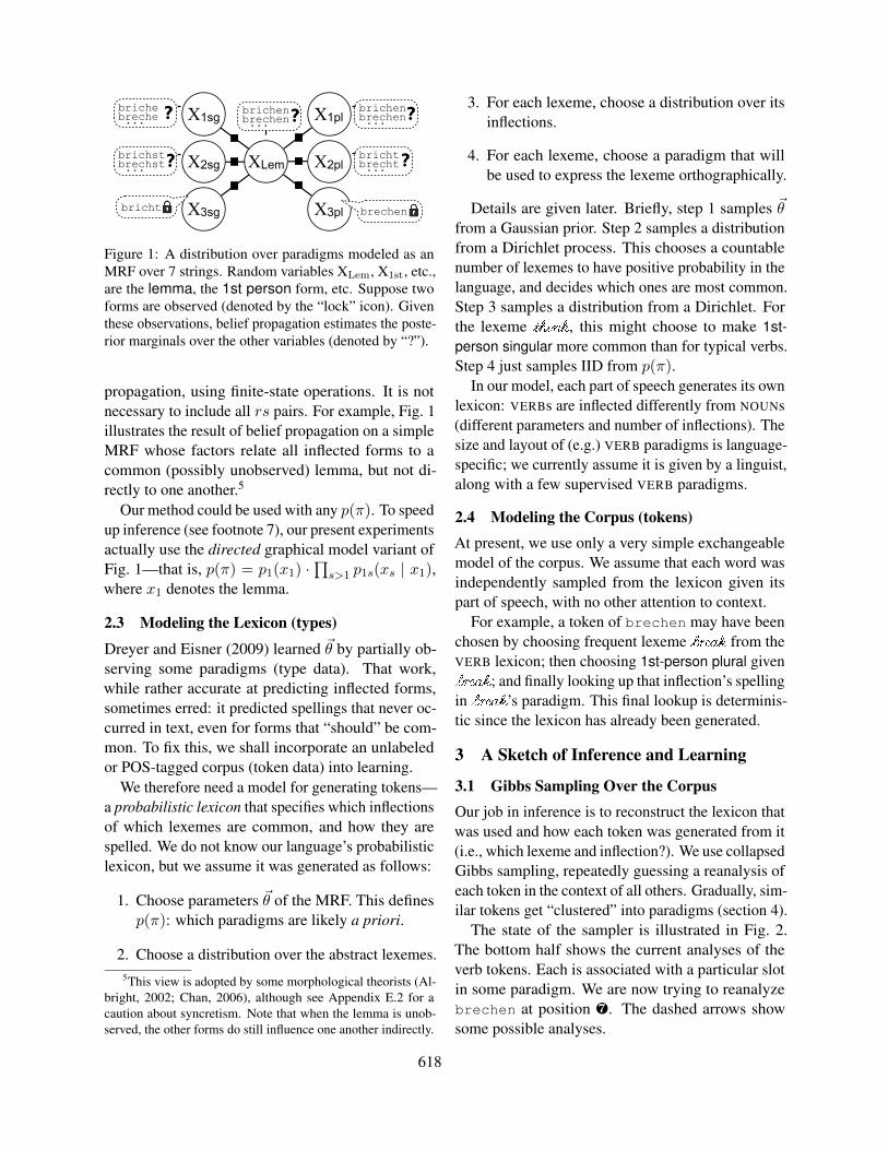
Figure 1: A distribution over paradigms modeled as anMRF over 7 strings. Random variables XLem, X1st, etc.,are the lemma, the 1st person form, etc. Suppose twoforms are observed (denoted by the “lock” icon). Giventhese observations, belief propagation estimates the poste-rior marginals over the other variables (denoted by “?”).

propagation, using finite-state operations. It is notnecessary to include all rs pairs. For example, Fig. 1illustrates the result of belief propagation on a simpleMRF whose factors relate all inflected forms to acommon (possibly unobserved) lemma, but not di-rectly to one another.5

Our method could be used with any p(π). To speedup inference (see footnote 7), our present experimentsactually use the directed graphical model variant ofFig. 1—that is, p(π) = p1(x1) ·

∏s>1 p1s(xs | x1),

where x1 denotes the lemma.

2.3 Modeling the Lexicon (types)

Dreyer and Eisner (2009) learned ~θ by partially ob-serving some paradigms (type data). That work,while rather accurate at predicting inflected forms,sometimes erred: it predicted spellings that never oc-curred in text, even for forms that “should” be com-mon. To fix this, we shall incorporate an unlabeledor POS-tagged corpus (token data) into learning.

We therefore need a model for generating tokens—a probabilistic lexicon that specifies which inflectionsof which lexemes are common, and how they arespelled. We do not know our language’s probabilisticlexicon, but we assume it was generated as follows:

1. Choose parameters ~θ of the MRF. This definesp(π): which paradigms are likely a priori.

2. Choose a distribution over the abstract lexemes.5This view is adopted by some morphological theorists (Al-

bright, 2002; Chan, 2006), although see Appendix E.2 for acaution about syncretism. Note that when the lemma is unob-served, the other forms do still influence one another indirectly.

3. For each lexeme, choose a distribution over itsinflections.

4. For each lexeme, choose a paradigm that willbe used to express the lexeme orthographically.

Details are given later. Briefly, step 1 samples ~θfrom a Gaussian prior. Step 2 samples a distributionfrom a Dirichlet process. This chooses a countablenumber of lexemes to have positive probability in thelanguage, and decides which ones are most common.Step 3 samples a distribution from a Dirichlet. Forthe lexeme �t�h�i�n�k, this might choose to make 1st-person singular more common than for typical verbs.Step 4 just samples IID from p(π).

In our model, each part of speech generates its ownlexicon: VERBs are inflected differently from NOUNs(different parameters and number of inflections). Thesize and layout of (e.g.) VERB paradigms is language-specific; we currently assume it is given by a linguist,along with a few supervised VERB paradigms.

2.4 Modeling the Corpus (tokens)At present, we use only a very simple exchangeablemodel of the corpus. We assume that each word wasindependently sampled from the lexicon given itspart of speech, with no other attention to context.

For example, a token of brechen may have beenchosen by choosing frequent lexeme �b&r��a�k from theVERB lexicon; then choosing 1st-person plural given�b&r��a�k; and finally looking up that inflection’s spellingin �b&r��a�k’s paradigm. This final lookup is determinis-tic since the lexicon has already been generated.

3 A Sketch of Inference and Learning

3.1 Gibbs Sampling Over the CorpusOur job in inference is to reconstruct the lexicon thatwas used and how each token was generated from it(i.e., which lexeme and inflection?). We use collapsedGibbs sampling, repeatedly guessing a reanalysis ofeach token in the context of all others. Gradually, sim-ilar tokens get “clustered” into paradigms (section 4).

The state of the sampler is illustrated in Fig. 2.The bottom half shows the current analyses of theverb tokens. Each is associated with a particular slotin some paradigm. We are now trying to reanalyzebrechen at position ¼. The dashed arrows showsome possible analyses.

618

singular plural

1st

2nd

3rd bricht

brichstbrechst... ?

brichebreche... ?

brechen

brichtbrecht... ?

brichenbrechen... ?

springstsprengst... ?

springesprenge... ?

springtsprengt... ?

springensprengen...

springensprengen...

1 3

Index i 2PRON

4NOUN

6PREPPOS ti

Infl si

Spell wi

Lex �i

1VERB

3rd sg.bricht

5VERB

2nd pl.springt

3VERB

3rd pl.brechen

??

5

Lexicon

Corpus

?

...

?

?

springt

7VERB

1st pl.

...brechen... ... ...

3rd pl.

Figure 2: A state of the Gibbs sampler (note that theassumed generative process runs roughly top-to-bottom).Each corpus token i has been tagged with part of speech ti,lexeme `i and inflection si. Token ¶ has been tagged as�b&r��a�k and 3rd sg., which locked the corresponding typespelling in the paradigm to the spelling w1 = bricht;similarly for ¸ and º. Now w7 is about to be reanalyzed.

The key intuition is that the current analyses of theother verb tokens imply a posterior distribution overthe VERB lexicon, shown in the top half of the figure.

First, because of the current analyses of ¶ and ¸,the 3rd-person spellings of �b&r��a�k are already con-strained to match w1 and w3 (the “lock” icon).

Second, belief propagation as in Fig. 1 tells uswhich other inflections of �b&r��a�k (the “?” icon) areplausibly spelled as brechen, and how likely theyare to be spelled that way.

Finally, the fact that other tokens are associatedwith �b&r��a�k suggest that this is a popular lexeme, mak-ing it a plausible explanation of ¼ as well. (This isthe “rich get richer” property of the Chinese restau-rant process; see section 6.6.) Furthermore, certaininflections of �b&r��a�k appear to be especially popular.

In short, given the other analyses, we know whichinflected lexemes in the lexicon are likely, and howlikely each one is to be spelled as brechen. This letsus compute the relative probabilities of the possibleanalyses of token ¼, so that the Gibbs sampler canaccordingly choose one of these analyses at random.

3.2 Monte Carlo EM Training of ~θ

For a given ~θ, this Gibbs sampler converges to theposterior distribution over analyses of the full corpus.To improve our ~θ estimate, we periodically adjust ~θto maximize or increase the probability of the mostrecent sample(s). For example, having tagged w5 =

springt as s5 = 2nd-person plural may strengthenour estimated probability that 2nd-person spellingstend to end in -t. That revision to ~θ, in turn, willinfluence future moves of the sampler.

If the sampler is run long enough between calls tothe ~θ optimizer, this is a Monte Carlo EM procedure(see end of section 1.2). It uses the data to optimize alanguage-specific prior p(π) over paradigms—an em-pirical Bayes approach. (A fully Bayesian approachwould resample ~θ as part of the Gibbs sampler.)

3.3 Collapsed Representation of the Lexicon

The lexicon is collapsed out of our sampler, in thesense that we do not represent a single guess about theinfinitely many lexeme probabilities and paradigms.What we store about the lexicon is information aboutits full posterior distribution: the top half of Fig. 2.

Fig. 2 names its lexemes as �b&r��a�k and �j�u�m�p for ex-pository purposes, but of course the sampler cannotreconstruct such labels. Formally, these labels are col-lapsed out, and we represent lexemes as anonymousobjects. Tokens ¶ and ¸ are tagged with the sameanonymous lexeme (which will correspond to sittingat the same table in a Chinese restaurant process).

For each lexeme ` and inflection s, we maintainpointers to any tokens currently tagged with the slot(`, s). We also maintain an approximate marginaldistribution over the spelling of that slot:6

1. If (`, s) points to at least one token i, then weknow (`, s) is spelled as wi (with probability 1).

2. Otherwise, the spelling of (`, s) is not known.But if some spellings in `’s paradigm are known,store a truncated distribution that enumerates the25 most likely spellings for (`, s), according toloopy belief propagation within the paradigm.

3. Otherwise, we have observed nothing about `:it is currently unused. All such ` share the samemarginal distribution over spellings of (`, s):the marginal of the prior p(π). Here a 25-bestlist could not cover all plausible spellings. In-stead we store a probabilistic finite-state lan-guage model that approximates this marginal.7

6Cases 1 and 2 below must in general be updated whenevera slot switches between having 0 and more than 0 tokens. Cases2 and 3 must be updated when the parameters ~θ change.

7This character trigram model is fast to build if p(π) is de-

619

A hash table based on cases 1 and 2 can now beused to rapidly map any word w to a list of slots ofexisting lexemes that might plausibly have generatedw. To ask whether w might instead be an inflection sof a novel lexeme, we score w using the probabilisticfinite-state automata from case 3, one for each s.

The Gibbs sampler randomly chooses one of theseanalyses. If it chooses the “novel lexeme” option,we create an arbitrary new lexeme object in mem-ory. The number of explicitly represented lexemes isalways finite (at most the number of corpus tokens).

4 Interpretation as a Mixture Model

It is common to cluster points in Rn by assumingthat they were generated from a mixture of Gaussians,and trying to reconstruct which points were generatedfrom the same Gaussian.

We are similarly clustering word tokens by assum-ing that they are generated from a mixture of weightedparadigms. After all, each word token was obtainedby randomly sampling a weighted paradigm (i.e., acluster) and then randomly sampling a word from it.

Just as each Gaussian in a Gaussian mixture isa distribution over all points Rn, each weightedparadigm is a distribution over all spellings Σ∗ (butassigns probability > 0 to only a finite subset of Σ∗).

Inference under our model clusters words togetherby tagging them with the same lexeme. It tends togroup words that are “similar” in the sense that thebase distribution p(π) predicts that they would tendto co-occur within a paradigm. Suppose a corpuscontains several unlikely but similar tokens, suchas discombobulated and discombobulating.A language might have one probable lexeme fromwhose paradigm all these words were sampled. It ismuch less likely to have several probable lexemes thatall coincidentally chose spellings that started withdiscombobulat-. Generating discombobulat-

only once is cheaper (especially for such a long pre-fix), so the former explanation has higher probability.This is like explaining nearby points in Rn as sam-ples from the same Gaussian. Of course, our modelis sensitive to more than shared prefixes, and it doesnot merely cluster words into a paradigm but assignsthem to particular inflectional slots in the paradigm.fined as at the end of section 2.2. If not, one could still try beliefpropagation; or one could approximate by estimating a languagemodel from the spellings associated with slot s by cases 1 and 2.

4.1 The Dirichlet Process Mixture Model

Our mixture model uses an infinite number of mix-ture components. This avoids placing a prior boundon the number of lexemes or paradigms in the lan-guage. We assume that a natural language has aninfinite lexicon, although most lexemes have suffi-ciently low probability that they have not been usedin our training corpus or even in human history (yet).

Our specific approach corresponds to a Bayesiantechnique, the Dirichlet process mixture model. Ap-pendix A (supplementary material) explains theDPMM and discusses it in our context.

The DPMM would standardly be presented as gen-erating a distribution over countably many Gaussiansor paradigms. Our variant in section 2.3 instead brokethis into two steps: it first generated a distributionover countably many lexemes (step 2), and then gen-erated a weighted paradigm for each lexeme (steps3–4). This construction keeps distinct lexemes sepa-rate even if they happen to have identical paradigms(polysemy). See Appendix A for a full discussion.

5 Formal Notation

5.1 Value Types

We now describe our probability model in more for-mal detail. It considers the following types of mathe-matical objects. (We use consistent lowercase lettersfor values of these types, and consistent fonts forconstants of these types.)

A word w, such as broken, is a finite string ofany length, over some finite, given alphabet Σ.

A part-of-speech tag t, such as VERB, is an ele-ment of a certain finite set T , which in this paper weassume to be given.

An inflection s,8 such as past participle, is an ele-ment of a finite set St. A token’s part-of-speech tagt ∈ T determines its set St of possible inflections.For tags that do not inflect, |St| = 1. The sets Stare language-specific, and we assume in this paperthat they are given by a linguist rather than learned.A linguist also specifies features of the inflections:the grid layout in Table 1 shows that 4 of the 12inflections in SVERB share the “2nd-person” feature.

8We denote inflections by s because they represent “slots” inparadigms (or, in the metaphor of section 6.7, “seats” at tables ina Chinese restaurant). These slots (or seats) are filled by words.

620

A paradigm for t ∈ T is a mapping π : St → Σ∗,specifying a spelling for each inflection in St. Table 1shows one VERB paradigm.

A lexeme ` is an abstract element of some lexicalspace L. Lexemes have no internal semantic struc-ture: the only question we can ask about a lexeme iswhether it is equal to some other lexeme. There is noupper bound on how many lexemes can be discoveredin a text corpus; L is infinite.

5.2 Random Quantities

Our generative model of the corpus is a joint probabil-ity distribution over a collection of random variables.We describe them in the same order as section 1.2.

Tokens: The corpus is represented by token vari-ables. In our setting the sequence of words ~w =w1, . . . , wn ∈ Σ∗ is observed, along with n. Wemust recover the corresponding part-of-speech tags~t = t1, . . . , tn ∈ T , lexemes ~̀ = `1, . . . , `n ∈ L,and inflections ~s = s1, . . . , sn, where (∀i)si ∈ Sti .

Types: The lexicon is represented by typevariables. For each of the infinitely many lex-emes ` ∈ L, and each t ∈ T , the paradigmπt,` is a function St → Σ∗. For example,Table 1 shows a possible value πVERB,�b&r��a�k.The various spellings in the paradigm, such asπVERB,�b&r��a�k(1st-person sing. pres.)=breche, arestring-valued random variables that are correlatedwith one another.

Since the lexicon is to be probabilistic (section 2.3),Gt(`) denotes tag t’s distribution over lexemes ` ∈L, while Ht,`(s) denotes the tagged lexeme (t, `)’sdistribution over inflections s ∈ St.

Grammar: Global properties of the language arecaptured by grammar variables that cut across lex-ical entries: our parameters ~θ that describe typicalinflectional alternations, plus parameters ~φt, αt, α′t, ~τ(explained below). Their values control the overallshape of the probabilistic lexicon that is generated.

6 The Formal Generative Model

We now fully describe the generative process thatwas sketched in section 2. Step by step, it randomlychooses an assignment to all the random variables ofsection 5.2. Thus, a given assignment’s probability—which section 3’s algorithms consult in order to re-sample or improve the current assignment—is the

product of the probabilities of the individual choices,as described in the sections below. (Appendix Bprovides a drawing of this as a graphical model.)

6.1 Grammar Variables p(~θ), p(−→φt), p(αt), p(α′t)First select the grammar variables from a prior. (Wewill see below how these variables get used.) Ourexperiments used fairly flat priors. Each weight in ~θor−→φt is drawn IID from N (0, 10), and each αt or α′t

from a Gamma with mode 10 and variance 1000.

6.2 Paradigms p(πt,` | ~θ)For each t ∈ T , let Dt(π) denote the distributionover paradigms that was presented in section 2.2(where it was called p(π)). Dt is fully specified byour graphical model for paradigms of part of speecht, together with its parameters ~θ as generated above.

This is the linguistic core of our model. It consid-ers spellings: DVERB describes what verb paradigmstypically look like in the language (e.g., Table 1).

Parameters in ~θ may be shared across parts ofspeech t. These “backoff” parameters capture gen-eral phonotactics of the language, such as prohibitedletter bigrams or plausible vowel changes.

For each possible tagged lexeme (t, `), we nowdraw a paradigm πt,` fromDt. Most of these lexemeswill end up having probability 0 in the language.

6.3 Lexical Distributions p(Gt | αt)We now formalize section 2.3. For each t ∈ T , thelanguage has a distribution Gt(`) over lexemes. Wedraw Gt from a Dirichlet process DP(G,αt), whereG is the base distribution over L, and αt > 0 isa concentration parameter generated above. If αtis small, then Gt will tend to have the property thatmost of its probability mass falls on relatively fewof the lexemes in Lt def

= {` ∈ L : Gt(`) > 0}. Aclosed-class tag is one whose αt is especially small.

For G to be a uniform distribution over an infinitelexeme set L, we need L to be uncountable.9 How-ever, it turns out10 that with probability 1, each Ltis countably infinite, and all the Lt are disjoint. Soeach lexeme ` ∈ L is selected by at most one tag t.

9For example, L def= [0, 1], so that �b&r��a�k is merely a sugges-

tive nickname for a lexeme such as 0.2538159.10This can be seen by considering the stick-breaking construc-

tion of the Dirichlet process that (Sethuraman, 1994; Teh et al.,2006). A separate stick is broken for each Gt. See Appendix A.

621

6.4 Inflectional Distributions p(Ht,` |−→φt, α′t)

For each tagged lexeme (t, `), the language specifiessome distribution Ht,` over its inflections.

First we construct backoff distributions Ht that areindependent of `. For each tag t ∈ T , let Ht be somebase distribution over St. As St could be large insome languages, we exploit its grid structure (Table 1)to reduce the number of parameters of Ht. We takeHt to be a log-linear distribution with parameters

−→φt

that refer to features of inflections. E.g., the 2nd-person inflections might be systematically rare.

Now we model each Ht,` as an independent drawfrom a finite-dimensional Dirichlet distribution withmeanHt and concentration parameter α′t. E.g., �t�h�i�n�kmight be biased toward 1st-person sing. present.

6.5 Part-of-Speech Tag Sequence p(~t | ~τ)

In our current experiments, ~t is given. But in general,to discover tags and inflections simultaneously, wecan suppose that the tag sequence ~t (and its length n)are generated by a Markov model, with tag bigram ortrigram probabilities specified by some parameters ~τ .

6.6 Lexemes p(`i | Gti)We turn to section 2.4. A lexeme token depends onits tag: draw `i from Gti , so p(`i | Gti) = Gti(`i).

6.7 Inflections p(si | Hti,`i)

An inflection slot depends on its tagged lexeme: wedraw si from Hti,`i , so p(si | Hti,`i) = Hti,`i(si).

6.8 Spell-out p(wi | πti,`i(si))Finally, we generate the word wi through a determin-istic spell-out step.11 Given the tag, lexeme, and in-flection at position i, we generate the word wi simplyby looking up its spelling in the appropriate paradigm.So p(wi | πti,`i(si)) is 1 if wi = πti,`i(si), else 0.

6.9 Collapsing the AssignmentAgain, a full assignment’s probability is the productof all the above factors (see drawing in Appendix B).

11To account for typographical errors in the corpus, the spell-out process could easily be made nondeterministic, with theobserved word wi derived from the correct spelling πti,`i(si)by a noisy channel model (e.g., (Toutanova and Moore, 2002))represented as a WFST. This would make it possible to analyzebrkoen as a misspelling of a common or contextually likelyword, rather than treating it as an unpronounceable, irregularlyinflected neologism, which is presumably less likely.

But computationally, our sampler’s state leaves theGt unspecified. So its probability is the integral ofp(assignment) over all possible Gt. As Gt appearsonly in the factors from headings 6.3 and 6.6, we canjust integrate it out of their product, to get a collapsedsub-model that generates p(~̀ | ~t, ~α) directly:∫

GADJ

· · ·∫

GVERB

dG

(∏

t∈Tp(Gt | αt)

)(n∏

i=1

p(`i | Gti))

= p(~̀ | ~t, ~α) =n∏

i=1

p(`i | `1, . . . `i−1 ~t, ~α)

where it turns out that the factor that generates `i isproportional to |{j < i : `j = `i and tj = ti}| if thatinteger is positive, else proportional to αtiG(`i).

Metaphorically, each tag t is a Chinese restaurantwhose tables are labeled with lexemes. The tokensare hungry customers. Each customer i = 1, 2, . . . , nenters restaurant ti in turn, and `i denotes the labelof the table she joins. She picks an occupied tablewith probability proportional to the number of pre-vious customers already there, or with probabilityproportional to αti she starts a new table whose labelis drawn from G (it is novel with probability 1, sinceG gives infinitesimal probability to each old label).

Similarly, we integrate out the infinitely manylexeme-specific distributionsHt,` from the product of6.4 and 6.7, replacing it by the collapsed distribution

p(~s | ~̀,~t,−→φt,−→α′) [recall that

−→φt determines Ht]

=

n∏

i=1

p(si | s1, . . . si−1, ~̀,~t,−→φt,−→α′)

where the factor for si is proportional to |{j < i :sj = si and (tj , `j) = (ti, `i)}|+ α′tiHti(si).

Metaphorically, each table ` in Chinese restaurantt has a fixed, finite set of seats corresponding to theinflections s ∈ St. Each seat is really a bench thatcan hold any number of customers (tokens). Whencustomer i chooses to sit at table `i, she also choosesa seat si at that table (see Fig. 2), choosing either analready occupied seat with probability proportional tothe number of customers already in that seat, or elsea random seat (sampled from Hti and not necessarilyempty) with probability proportional to α′ti .

7 Inference and Learning

As section 3 explained, the learner alternates betweena Monte Carlo E step that uses Gibbs sampling to

622

sample from the posterior of (~s, ~̀,~t) given ~w and thegrammar variables, and an M step that adjusts thegrammar variables to maximize the probability of the(~w,~s, ~̀,~t) samples given those variables.

7.1 Block Gibbs SamplingAs in Gibbs sampling for the DPMM, our sampler’sbasic move is to reanalyze token i (see section 3).This corresponds to making customer i invisible andthen guessing where she is probably sitting—whichrestaurant t, table `, and seat s?—given knowledgeof wi and the locations of all other customers.12

Concretely, the sampler guesses location (ti, `i, si)with probability proportional to the product of• p(ti | ti−1, ti+1, ~τ) (from section 6.5)• the probability (from section 6.9) that a new cus-

tomer in restaurant ti chooses table `i, given theother customers in that restaurant (and αti)

13

• the probability (from section 6.9) that a newcustomer at table `i chooses seat si, given theother customers at that table (and

−→φti and α′ti)

13

• the probability (from section 3.3’s belief propa-gation) that πti,`i(si) = wi (given ~θ).

We sample only from the (ti, `i, si) candidates forwhich the last factor is non-negligible. These arefound with the hash tables and FSAs of section 3.3.

7.2 Semi-Supervised SamplingOur experiments also consider the semi-supervisedcase where a few seed paradigms—type data—arefully or partially observed. Our samples should alsobe conditioned on these observations. We assumethat our supervised list of observed paradigms wasgenerated by sampling from Gt.14 We can modifyour setup for this case: certain tables have a hostwho dictates the spelling of some seats and attractsappropriate customers to the table. See Appendix C.

7.3 Parameter GradientsAppendix D gives formulas for the M step gradients.

12Actually, to improve mixing time, we choose a currentlyactive lexeme ` uniformly at random, make all customers {i :`i = `} invisible, and sequentially guess where they are sitting.

13This is simple to find thanks to the exchangeability of theCRP, which lets us pretend that i entered the restaurant last.

14Implying that they are assigned to lexemes with non-negligible probability. We would learn nothing from a list ofmerely possible paradigms, since Lt is infinite and every con-ceivable paradigm is assigned to some ` ∈ Lt (in fact many!).

50 seed paradigms 100 seed paradigmsCorpus size 0 106 107 0 106 107

Accuracy 89.9 90.6 90.9 91.5 92.0 92.2Edit dist. 0.20 0.19 0.18 0.18 0.17 0.17

Table 2: Whole-word accuracy and edit distance of pre-dicted inflection forms given the lemma. Edit distance tothe correct form is measured in characters. Best numbersper set of seed paradigms in bold (statistically signifi-cant on our large test set under a paired permutation test,p < 0.05). Appendix E breaks down these results perinflection and gives an error analysis and other statistics.

8 Experiments

8.1 Experimental DesignWe evaluated how well our model learns Germanverbal morphology. As corpus we used the first 1million or 10 million words from WaCky (Baroniet al., 2009). For seed and test paradigms we usedverbal inflectional paradigms from the CELEX mor-phological database (Baayen et al., 1995). We fullyobserved the seed paradigms. For each test paradigm,we observed the lemma type (Appendix C) and eval-uated how well the system completed the other 21forms (see Appendix E.2) in the paradigm.

We simplified inference by fixing the POS tagsequence to the automatic tags delivered with theWaCky corpus. The result that we evaluated for eachvariable was the value whose probability, averagedover the entire Monte Carlo EM run,15 was highest.For more details, see (Dreyer, 2011).

All results are averaged over 10 different train-ing/test splits of the CELEX data. Each split sampled100 paradigms as seed data and used the remain-ing 5,415 paradigms for evaluation.16 From the 100paradigms, we also sampled 50 to obtain results withsmaller seed data.17

8.2 ResultsType-based Evaluation. Table 2 shows the resultsof predicting verb inflections, when running with nocorpus, versus with an unannotated corpus of size 106

and 107 words. Just using 50 seed paradigms, but

15This includes samples from before ~θ has converged, some-what like the voted perceptron (Freund and Schapire, 1999).

16100 further paradigms were held out for future use.17Since these seed paradigms are sampled uniformly from a

set of CELEX paradigms, most of them are regular. We actuallyonly used 90 and 40 for training, reserving 10 as developmentdata for sanity checks and for deciding when to stop.

623

Bin Frequency # Verb Forms1 0–9 116,7762 10–99 4,6233 100–999 1,0484 1,000–9,999 955 10,000– 10

all any 122,552

Table 3: The inflected verb forms from 5,615 inflectionalparadigms, split into 5 token frequency bins. The frequen-cies are based on the 10-million word corpus.

no corpus, gives an accuracy of 89.9%. By addinga corpus of 10 million words we reduce the errorrate by 10%, corresponding to a one-point increasein absolute accuracy to 90.9%. A similar trend canbe seen when we use more seed paradigms. Sim-ply training on 100 seed paradigms, but not using acorpus, results in an accuracy of 91.5%. Adding acorpus of 10 million words to these 100 paradigms re-duces the error rate by 8.3%, increasing the absoluteaccuracy to 92.2%. Compared to the large corpus,the smaller corpus of 1 million words goes more thanhalf the way; it results in error reductions of 6.9%(50 seed paradigms) and 5.8% (100 seed paradigms).Larger unsupervised corpora should help by increas-ing coverage even more, although Zipf’s law impliesa diminishing rate of return.18

We also tested a baseline that simply inflects eachmorphological form according to the basic regularGerman inflection pattern; this reaches an accuracyof only 84.5%.

Token-based Evaluation. We now split our resultsinto different bins: how well do we predict thespellings of frequently expressed (lexeme, inflection)pairs as opposed to rare ones? For example, the thirdperson singular indicative of �g�i�v� (geben) is usedsignificantly more often than the second person pluralsubjunctive of �b$a�s�k (aalen);19 they are in differentfrequency bins (Table 3). The more frequent a formis in text, the more likely it is to be irregular (Jurafskyet al., 2000, p. 49).

The results in Table 4 show: Adding a corpus ofeither 1 or 10 million words increases our predictionaccuracy across all frequency bins, often dramati-cally. All methods do best on the huge number of

18Considering the 63,778 distinct spellings from all of our5,615 CELEX paradigms, we find that the smaller corpus con-tains 7,376 spellings and the 10× larger corpus contains 13,572.

19See Appendix F for how this was estimated from text.

50 seed paradigms 100 seed paradigmsBin 0 106 107 0 106 107

1 90.5 91.0 91.3 92.1 92.4 92.62 78.1 84.5 84.4 80.2 85.5 85.13 71.6 79.3 78.1 73.3 80.2 79.14 57.4 61.4 61.8 57.4 62.0 59.95 20.7 25.0 25.0 20.7 25.0 25.0

all 52.6 57.5 57.8 53.4 58.5 57.8all (e.d.) 1.18 1.07 1.03 1.16 1.02 1.01

Table 4: Token-based analysis: Whole-word accuracy re-sults split into different frequency bins. In the last tworows, all predictions are included, weighted by the fre-quency of the form to predict. Last row is edit distance.

rare forms (Bin 1), which are mostly regular, andworst on on the 10 most frequent forms of the lan-guage (Bin 5). However, adding a corpus helps mostin fixing the errors in bins with more frequent andhence more irregular verbs: in Bins 2–5 we observeimprovements of up to almost 8% absolute percent-age points. In Bin 1, the no-corpus baseline is alreadyrelatively strong.

Surprisingly, while we always observe gains fromusing a corpus, the gains from the 10-million-wordcorpus are sometimes smaller than the gains from the1-million-word corpus, except in edit distance. Why?The larger corpus mostly adds new infrequent types,biasing ~θ toward regular morphology at the expenseof irregular types. A solution might be to model irreg-ular classes with separate parameters, using the latentconjugation-class model of Dreyer et al. (2008).

Note that, by using a corpus, we even improveour prediction accuracy for forms and spellings thatare not found in the corpus, i.e., novel words. Thisis thanks to improved grammar parameters. In thetoken-based analysis above we have already seen thatprediction accuracy increases for rare forms (Bin 1).We add two more analyses that more explicitly showour performance on novel words. (a) We find allparadigms that consist of novel spellings only, i.e.none of the correct spellings can be found in thecorpus.20 The whole-word prediction accuracies forthe models that use corpus size 0, 1 million, and10 million words are, respectively, 94.0%, 94.2%,94.4% using 50 seed paradigms, and 95.1%, 95.3%,95.2% using 100 seed paradigms. (b) Another, sim-

20This is measured on the largest corpus used in inference, the10-million-word corpus, so that we can evaluate all models onthe same set of paradigms.

624

pler measure is the prediction accuracy on all formswhose correct spelling cannot be found in the 10-million-word corpus. Here we measure accuraciesof 91.6%, 91.8% and 91.8%, respectively, using 50seed paradigms. With 100 seed paradigms, we have93.0%, 93.4% and 93.1%. The accuracies for themodels that use a corpus are higher, but do not al-ways steadily increase as we increase the corpus size.

The token-based analysis we have conducted hereshows the strength of the corpus-based approach pre-sented in this paper. While the integrated graphi-cal models over strings (Dreyer and Eisner, 2009)can learn some basic morphology from the seedparadigms, the added corpus plays an important rolein correcting its mistakes, especially for the more fre-quent, irregular verb forms. For examples of specificerrors that the models make, see Appendix E.3.

9 Related Work

Our word-and-paradigm model seamlessly handlesnonconcatenative and concatenative morphologyalike, whereas most previous work in morphologicalknowledge discovery has modeled concatenative mor-phology only, assuming that the orthographic formof a word can be split neatly into stem and affixes—asimplifying asssumption that is convenient but oftennot entirely appropriate (Kay, 1987) (how should onesegment English stopping, hoping, or knives?).

In concatenative work, Harris (1955) finds mor-pheme boundaries and segments words accordingly,an approach that was later refined by Hafer andWeiss (1974), Déjean (1998), and many others. Theunsupervised segmentation task is tackled in theannual Morpho Challenge (Kurimo et al., 2010),where ParaMor (Monson et al., 2007) and Morfessor(Creutz and Lagus, 2005) are influential contenders.The Bayesian methods that Goldwater et al. (2006b,et seq.) use to segment between words might also beapplied to segment within words, but have no notionof paradigms. Goldsmith (2001) finds what he callssignatures—sets of affixes that are used with a givenset of stems, for example (NULL, -er, -ing, -s).Chan (2006) learns sets of morphologically relatedwords; he calls these sets paradigms but notes thatthey are not substructured entities, in contrast to theparadigms we model in this paper. His models arerestricted to concatenative and regular morphology.

Morphology discovery approaches that han-dle nonconcatenative and irregular phenomenaare more closely related to our work; they arerarer. Yarowsky and Wicentowski (2000) identifyinflection-root pairs in large corpora without supervi-sion. Using similarity as well as distributional clues,they identify even irregular pairs like take/took.Schone and Jurafsky (2001) and Baroni et al. (2002)extract whole conflation sets, like “abuse, abused,abuses, abusive, abusively, . . . ,” which mayalso be irregular. We advance this work by not onlyextracting pairs or sets of related observed words,but whole structured inflectional paradigms, in whichwe can also predict forms that have never been ob-served. On the other hand, our present model doesnot yet use contextual information; we regard this asa future opportunity (see Appendix G). Naradowskyand Goldwater (2009) add simple spelling rules tothe Bayesian model of (Goldwater et al., 2006a), en-abling it to handle some systematically nonconcate-native cases. Our finite-state transducers can handlemore diverse morphological phenomena.

10 Conclusions and Future Work

We have formulated a principled framework for si-multaneously obtaining morphological annotation,an unbounded morphological lexicon that fills com-plete structured morphological paradigms with ob-served and predicted words, and parameters of a non-concatenative generative morphology model.

We ran our sampler over a large corpus (10 millionwords), inferring everything jointly and reducing theprediction error for morphological inflections by upto 10%. We observed that adding a corpus increasesthe absolute prediction accuracy on frequently occur-ring morphological forms by up to almost 8%. Futureextensions to the model could leverage token contextfor further improvements (Appendix G).

We believe that a major goal of our field should beto build full-scale explanatory probabilistic modelsof language. While we focus here on inflectionalmorphology and evaluate the results in isolation, weregard the present work as a significant step towarda larger generative model under which Bayesianinference would reconstruct other relationships aswell (e.g., inflectional, derivational, and evolution-ary) among the words in a family of languages.

625

References

A. C. Albright. 2002. The Identification of Bases inMorphological Paradigms. Ph.D. thesis, University ofCalifornia, Los Angeles.

D. Aldous. 1985. Exchangeability and related topics.École d’été de probabilités de Saint-Flour XIII, pages1–198.

C. E. Antoniak. 1974. Mixtures of Dirichlet processeswith applications to Bayesian nonparametric problems.Annals of Statistics, 2(6):1152–1174.

R. H Baayen, R. Piepenbrock, and L. Gulikers. 1995. TheCELEX lexical database (release 2)[cd-rom]. Philadel-phia, PA: Linguistic Data Consortium, University ofPennsylvania [Distributor].

M. Baroni, J. Matiasek, and H. Trost. 2002. Unsuperviseddiscovery of morphologically related words based onorthographic and semantic similarity. In Proc. of theACL-02 Workshop on Morphological and PhonologicalLearning, pages 48–57.

M. Baroni, S. Bernardini, A. Ferraresi, and E. Zanchetta.2009. The WaCky Wide Web: A collection of verylarge linguistically processed web-crawled corpora.Language Resources and Evaluation, 43(3):209–226.

David Blackwell and James B. MacQueen. 1973. Fergu-son distributions via Pòlya urn schemes. The Annals ofStatistics, 1(2):353–355, March.

David M. Blei and Peter I. Frazier. 2010. Distance-dependent Chinese restaurant processes. In Proc. ofICML, pages 87–94.

E. Chan. 2006. Learning probabilistic paradigms formorphology in a latent class model. In Proceedings ofthe Eighth Meeting of the ACL Special Interest Groupon Computational Phonology at HLT-NAACL, pages69–78.

M. Creutz and K. Lagus. 2005. Unsupervised morphemesegmentation and morphology induction from text cor-pora using Morfessor 1.0. Computer and InformationScience, Report A, 81.

H. Déjean. 1998. Morphemes as necessary conceptfor structures discovery from untagged corpora. InProc. of the Joint Conferences on New Methods inLanguage Processing and Computational Natural Lan-guage Learning, pages 295–298.

Markus Dreyer and Jason Eisner. 2009. Graphical modelsover multiple strings. In Proc. of EMNLP, Singapore,August.

Markus Dreyer, Jason Smith, and Jason Eisner. 2008.Latent-variable modeling of string transductions withfinite-state methods. In Proc. of EMNLP, Honolulu,Hawaii, October.

Markus Dreyer. 2011. A Non-Parametric Model for theDiscovery of Inflectional Paradigms from Plain Text

Using Graphical Models over Strings. Ph.D. thesis,Johns Hopkins University.

T.S. Ferguson. 1973. A Bayesian analysis of some non-parametric problems. The annals of statistics, 1(2):209–230.

Y. Freund and R. Schapire. 1999. Large margin classifica-tion using the perceptron algorithm. Machine Learning,37(3):277–296.

J. Goldsmith. 2001. Unsupervised learning of the mor-phology of a natural language. Computational Linguis-tics, 27(2):153–198.

S. Goldwater, T. Griffiths, and M. Johnson. 2006a. In-terpolating between types and tokens by estimatingpower-law generators. In Proc. of NIPS, volume 18,pages 459–466.

S. Goldwater, T. L. Griffiths, and M. Johnson. 2006b.Contextual dependencies in unsupervised word seg-mentation. In Proc. of COLING-ACL.

P.J. Green. 1995. Reversible jump Markov chain MonteCarlo computation and Bayesian model determination.Biometrika, 82(4):711.

M. A Hafer and S. F Weiss. 1974. Word segmentationby letter successor varieties. Information Storage andRetrieval, 10:371–385.

Z. S. Harris. 1955. From phoneme to morpheme. Lan-guage, 31(2):190–222.

G.E. Hinton. 2002. Training products of experts by min-imizing contrastive divergence. Neural Computation,14(8):1771–1800.

Klara Janecki. 2000. 300 Polish Verbs. Barron’s Educa-tional Series.

E. T. Jaynes. 2003. Probability Theory: The Logic ofScience. Cambridge Univ Press. Edited by Larry Bret-thorst.

D. Jurafsky, J. H. Martin, A. Kehler, K. Vander Linden,and N. Ward. 2000. Speech and Language Processing:An Introduction to Natural Language Processing, Com-putational Linguistics, and Speech Recognition. MITPress.

M. Kay. 1987. Nonconcatenative finite-state morphology.In Proc. of EACL, pages 2–10.

M. Kurimo, S. Virpioja, V. Turunen, and K. Lagus. 2010.Morpho Challenge competition 2005–2010: Evalua-tions and results. In Proc. of ACL SIGMORPHON,pages 87–95.

P. H. Matthews. 1972. Inflectional Morphology: A Theo-retical Study Based on Aspects of Latin Verb Conjuga-tion. Cambridge University Press.

Christian Monson, Jaime Carbonell, Alon Lavie, and LoriLevin. 2007. ParaMor: Minimally supervised induc-tion of paradigm structure and morphological analysis.In Proc. of ACL SIGMORPHON, pages 117–125, June.

626

J. Naradowsky and S. Goldwater. 2009. Improving mor-phology induction by learning spelling rules. In Proc.of IJCAI, pages 1531–1536.

J. Pitman and M. Yor. 1997. The two-parameter Poisson-Dirichlet distribution derived from a stable subordinator.Annals of Probability, 25:855–900.

P. Schone and D. Jurafsky. 2001. Knowledge-free induc-tion of inflectional morphologies. In Proc. of NAACL,volume 183, pages 183–191.

J. Sethuraman. 1994. A constructive definition of Dirich-let priors. Statistica Sinica, 4(2):639–650.

N. A. Smith, D. A. Smith, and R. W. Tromble. 2005.Context-based morphological disambiguation with ran-dom fields. In Proceedings of HLT-EMNLP, pages475–482, October.

G. T. Stump. 2001. Inflectional Morphology: A Theory ofParadigm Structure. Cambridge University Press.

Y.W. Teh, M.I. Jordan, M.J. Beal, and D.M. Blei. 2006.Hierarchical Dirichlet processes. Journal of the Ameri-can Statistical Association, 101(476):1566–1581.

Yee Whye Teh. 2006. A hierarchical Bayesian languagemodel based on Pitman-Yor processes. In Proc. ofACL.

K. Toutanova and R.C. Moore. 2002. Pronunciationmodeling for improved spelling correction. In Proc. ofACL, pages 144–151.

D. Yarowsky and R. Wicentowski. 2000. Minimally su-pervised morphological analysis by multimodal align-ment. In Proc. of ACL, pages 207–216, October.

627

This supplementary material consists of severalappendices. The main paper can be understood with-out them; but for the curious reader, the appendicesprovide additional background, details, results, anal-ysis, and discussion (see also (Dreyer, 2011)). Eachappendix is independent of the others, since differentappendices may be of interest to different readers.

A Dirichlet Process Mixture Models

Section 4 noted that morphology induction is ratherlike the clustering that is performed by inferenceunder a Dirichlet process mixture model (Antoniak,1974). The DPMM is trivially obtained from theDirichlet process (Ferguson, 1973), on which thereare many good tutorials. Our purpose in this appendixis

• to briefly present the DPMM in the concretesetting of morphology, for the interested reader;

• to clarify why and how we introduce abstractlexemes, obtaining a minor technical variant ofthe DPMM (section A.5).

The DPMM provides a Bayesian approach to non-parametric clustering. It is Bayesian because it speci-fies a prior over the mixture model that might havegenerated the data. It is non-parametric because thatmixture model uses an infinite number of mixturecomponents (in our setting, an infinite lexicon).

Generating a larger data sample tends to selectmore of these infinitely many components to generateactual data points. Thus, inference tends to use moreclusters to explain how a larger sample was generated.In our setting, the more tokens in our corpus, themore paradigms we will organize them into.

A.1 Parameters of a DPMMAssume that we are given a (usually infinite) set Lof possible mixture components. That is, each ele-ment of L is a distribution `(w) over some space ofobservable objects w. Commonly `(w) is a Gaussiandistribution over points w ∈ Rn. In our setting, `(w)is a weighted paradigm, which is a distribution (onewith finite support) over strings w ∈ Σ∗.

Notice that we are temporarily changing our no-tation. In the main paper, ` denotes an abstract lex-eme that is associated with a spelling πt,`(s) and aprobability Ht,`(s) for each slot s ∈ St. For the

moment, however, in order to present the DPMM,we are instead using ` to denote an actual mixturecomponent—the distribution over words obtainedfrom these spellings and probabilities. In section A.5we will motivate the alternative construction used inthe main paper, in which ` is just an index into theset of possible mixture components.

A DPMM is parameterized by a concentrationparameter α > 0 together with a base distributionG over the mixture components L. Thus, G stateswhat typical Gaussians or weighted paradigms oughtto look like.21 (What variances σ2 and means µ arelikely? What affixes and stem changes are likely?) Inour setting, this is a global property of the languageand is determined by the grammar parameters ~θ.

A.2 Sampling a Specific Mixture Model

To draw a specific mixture model from the DPMMprior, we can use a stick-breaking process. The ideais to generate an infinite sequence of mixture com-ponents `(1), `(2), . . . as IID samples from G. In oursetting, this is a sequence of weighted paradigms.

We then associate a probability βk > 0 with eachcomponent, where

∑∞k=1 βk = 1. These βk probabil-

ities serve as the mixture weights. They are chosensequentially, in a way that tends to decrease. Thus,the paradigms that fall early in the `(k) sequence tendto be the high-frequency paradigms of the language.These ` values do not necessarily have high priorprobability under G. However, a paradigm ` that isvery unlikely under G will probably not be chosenanywhere early in the `(k) sequence, and so will endup with a low probability.

Specifically: having already chosen β1, . . . , βk−1,we set βk to be the remaining probability mass1−∑k−1

i=1 βi times a random fraction in (0,1) that isdrawn IID from Beta(1, α).22 Metaphorically, hav-ing already broken k − 1 segments off a stick oflength 1, representing the total probability mass, wenow break off a random fraction of what is left of thestick. We label the new stick segment with `(k).

This distribution β over the integers yields a dis-tribution Gt over mixture components: Gt(`) =

21The traditional name for the base distribution is G0. Wedepart from this notation since we want to use the subscriptposition instead to distinguish draws from the DPMM, e.g., Gt.

22Equivalently, letting β′k be the random fraction, we candefine βk = β′k ·

∏k−1i=1 (1− β′i).

Supplementary material for: Markus Dreyer & Jason Eisner (2011),“Discovering morphological paradigms from plain text using a Dirichlet process mixture model,”

Proceedings of the Conference on Empirical Methods in Natural Language Processing (EMNLP)

∑k:`(k)=` βk, the probability of selecting a stick seg-

ment labeled with `. Clearly, this probability is posi-tive if and only if ` is in {`(1), `(2), . . .}, a countablesubset of L that is countably infinite provided that Ghas infinite support.

As Sethuraman (1994) shows, thisGt is distributedaccording to the Dirichlet process DP(G,α). Gt isa discrete distribution and tends to place its masson mixture components that have high probabilityunder G. In fact, the average value of Gt is exactlyG. However, Gt is not identical to G, and differentsamples Gt will differ considerably from one anotherif α is small.23 In short,G is the mean of the Dirichletprocess while α is inversely related to its variance.

A.3 α for a Natural Language LexiconWe expect α to be relatively small in our model,since a lexicon is idiosyncratic: Gt does not looktoo much like G. Many verb paradigms ` that wouldbe a priori reasonable in the language (large G(`))are in fact missing from the dictionary and are onlyavailable as neologisms (small Gt(`)). Conversely,irregular paradigms (small G(`)) are often selectedfor frequent use in the language (large Gt(`)).

On the other hand, small α implies that we willbreak off large stick segments and most of the proba-bility mass will rapidly be used up on a small numberof paradigms. This is not true: the distribution overwords in a language has a long tail (Zipf’s Law).In fact, regardless of α, Dirichlet processes nevercapture the heavy-tailed, power-law behavior that istypical of linguistic distributions. The standard solu-tion is to switch to the Pitman-Yor process (Pitmanand Yor, 1997; Teh, 2006), a variant on the Dirichletprocess that has an extra parameter to control theheaviness of the tail. We have not yet implementedthis simple improvement.

A.4 Sampling from the Mixture ModelThe distribution over paradigms, Gt, gives rise toa distribution over words, pt(w) =

∑`Gt(`) c(w).

To sample a word w from this distribution, one cansample a mixture component ` ∼ Gt and then a pointw ∼ `. This is what sections 6.6–6.8 do. To generatea whole corpus of n words, one must repeat thesetwo steps n times.

23As α→ 0, the expected divergence KL(Gt||G)→ H(G).As α→∞, on the other hand, the expected KL(Gt||G)→ 0.

For simplicity of notation, let us assume that t isfixed, so that all words are generated from the sameGt (i.e., they have the same part-of-speech tag).24

Thus, we need to sample a sequence`1, `2, . . . , `n ∼ Gt. Is there a way to do thiswithout explicitly representing the particular infinitemixture model Gt ∼ DP(G,α)? It does not matterhere that each `i is a mixture component. Whatmatters is that it is a sample ` from a sample Gtfrom a Dirichlet process. Hence we can use standardtechniques for working with Dirichlet processes.

The solution is the scheme known as a Chineserestaurant process (Blackwell and MacQueen, 1973;Aldous, 1985), as employed in section 6.9. Our n IIDdraws from Gt are conditionally independent givenGt (by definition), but they become interdependentif Gt is not observed. This is because `1, . . . , `i−1provide evidence about whatGt must have been. Thenext sample `i must then be drawn from the mean ofthis posterior over Gt (which becomes sharper andsharper as i increases and we gain knowledge of Gt).

It turns out that the posterior mean assigns to each` ∈ L a probability that is proportional to t(`) +αG(`), where t(`) is the number of previous samplesequal to `. The Chinese restaurant process samplesfrom this distribution by using the scheme describedin section 6.9.

For a given `, each table in the Chinese restaurantlabeled with ` corresponds to some stick segment kthat is labeled with `. However, unlike the stick seg-ment, the table does not record the value of k. It alsodoes not represent the segment length βk—althoughthe fraction of customers who are sitting at the tabledoes provide some information about βk, and theposterior distribution over βk gets sharper as morecustomers enter the restaurant. In short, the Chineserestaurant representation is more collapsed than thestick-breaking representation, since it does not recordGt nor a specific stick-breaking construction of Gt.

A.5 LexemesWe now make lexemes and inflections into first-classvariables of the model, which can be inferred (sec-tion 7), directly observed (Appendix C), modulatedby additional factors (Appendix G), or associated

24Recall that in reality, we switch among several Gt, onefor each part-of-speech tag t. In that case, we use Gti whensampling the word at position i.

with other linguistic information. The use of first-class lexemes also permits polysemy, where twolexemes remain distinct despite having the sameparadigm.

If we used the DPMM directly, our inference proce-dure would only assign a paradigm `i to each corpustoken i. Given our goals of doing morphological anal-ysis, this formalization is too weak on two grounds:

• We have ignored the structure of the paradigmby treating it as a mere distribution over strings(mixture component). We would like to recovernot only the paradigm that generated token ibut also the specific responsible slot si in thatparadigm.

• By tagging only with a paradigm and not with alexical item, we have failed to disambiguate ho-mographs. For example, `i says only that drewis a form of draw. It does not distinguish be-tween drawing a picture and drawing a sample,both of which use the same paradigm.25

Regarding the second point, one might object thatthe two senses of drew could be identified with dif-ferent weighted paradigms, which have the samespellings but differ slightly in their weights. How-ever, this escape hatch is not always available. Forexample, suppose we simplified our model by con-straining Ht,` to equal Ht. Then the different sensesof draw would have identical weighted paradigms,the weights being imposed by t, and they could nolonger be distinguished. To avoid such problems,we think it is prudent to design notation that refersdirectly to linguistic concepts like abstract lexemes.

Thus, we now switch to the variant view we pre-sented in the main paper, in which each ` ∈ L isan abstract lexeme rather than a mixture component.We still have Gt ∼ DP(G,α), but now G and Gtare distributions over abstract lexemes. The particu-lar mixture components are obtained by choosing astructured paradigm πt,` and weights Ht,` for eachabstract lexeme ` (sections 6.3–6.4). In principle, se-

25Of course, our current model is too weak to make suchsense distinctions successfully, since it does not yet considercontext. But we would like it to at least be able to representthese distinctions in its tagging. In future work (Appendix G)we would hope to consider context, without overhauling theframework and notation of the present paper.

mantic and subcategorization information could alsobe associated with the lexeme.

In our sampler, a newly created Chinese restauranttable ought to sample a label ` ∈ L from G. This isstraightforward but turns out to be unnecessary, sincethe particular value of ` does not matter in our model.All that matters is the information that we associatedwith ` above. In effect, ` is just an arbitrary pointerto the lexical entry containing this information. Thus,in practice, we collapse out the value ` and take thelexical entry information to be associated directlywith the Chinese restaurant table instead.26

We can identify lexemes with Chinese restauranttables in this way provided that G has no atoms (i.e.,any particular ` ∈ L has infinitesimal probabilityunder G), as is also true for the standard GaussianDPMM. Then, in the generative processes above, twotables (or two stick segments) never happen to choosethe same lexeme. So there is no possibility that asingle lexeme’s customers are split among multipletables. As a result, we never have to worry aboutcombining customers from multiple tables in order toestimate properties of a lexeme (e.g., when estimatingits paradigm by loopy belief propagation).

For concreteness, we can take lexeme space L tobe the uncountable set [0, 1] (see footnote 9), and letG be the uniform distribution over [0, 1]. However,these specific choices are not important, providedthat G has no atoms and the model does not makeany reference to the structure of L.

B Graphical Model Diagram

We provide in Fig. 3 a drawing of our graphicalmodel, corresponding to section 6.

The model is simpler than it appears. First, thevariables Dt, Ht, G, and wi are merely determinis-tic functions of their parents. Second, several of theedges denote only simple “switching variable” depen-dencies. These are the thin edges connecting corpusvariables `i, si, wi to the corpus variables above them.For example, `i is simply sampled from one of theGt distributions (section 6.6)—but specifically fromGti , so it also needs ti as a parent (thin edge). In the

26So, instead of storing the lexeme vector ~̀, which associatesa specific lexeme with each token, we only really store a partition(clustering) that says which tokens have the same lexeme. Thelexemes play the role of cluster labels, so the fact that they arenot identifiable and not stored is typical of a clustering problem.

� ∈ L

t ∈ T

Ht,�Ht

φt Dt

θ

Gt

ti−1 ti

�i

si

wi

i = 1..n

base

Gbase

πt,l

α�t

τ

Lexicon

Corpus

αt

Figure 3: A graphical model drawing of the generativemodel. As in Fig. 2, type variables are above and tokenvariables are below. Grammar variables are in blue. Al-though circles denote random variables, we label themwith values (such as `i) to avoid introducing new notation(such as Li) for the random variables.

same way, si is sampled from Hti,`i , and wi deter-ministically equals πti,`i(s).wi is observed, as shown by the shading. However,

the drawing does not show some observations men-tioned in section 8.1. First, πt,` is also observed forcertain seed paradigms (t, `). Second, our presentexperiments also constrain ti (to a value predicted byan automatic tagger), and then consider only those ifor which ti = VERB.

C Incorporating Known Paradigms

To constrain the inference and training, the methodis given a small set of known paradigms of the lan-guage (for each tag t). This should help us find areasonable initial value for ~θ. It can also be given apossibly larger set of incomplete known paradigms(section 7.2). In this appendix, we describe how thispartial supervision is interpreted and how it affectsinference.

Each supervised paradigm, whether complete or

incomplete, comes labeled with a lexeme such as�b&r��a�k. (Ordinarily these lexemes are distinct but thatis not required.) This labeling will make it possibleto inspect samples from the posterior and evaluateour system on how well it completed the incompleteparadigms of known lexemes (section 8.1), or usedknown lexemes to annotate word tokens.

In our experiments, each incomplete paradigmspecifies only the spelling of the lemma inflection.This special inflection is assumed not to be generatedin text (i.e., Ht(lemma) = 0). Our main reason forsupplying these partial paradigms is to aid evaluation,but it does also provides some weak supervision. Ad-ditional supervision of this kind could be obtainedthrough uninflected word lists, which are availablefor many languages.

Another source of incomplete paradigms wouldbe human informants. In an active learning setting,we might show humans some of the paradigms thatwe have reconstructed so far, and query them aboutforms to which we currently assign a high entropy ora high value-of-information.

At any rate, we should condition our inference onany data that we are given. In the standard semi-supervised setting, we would be given a partiallyannotated corpus (token data), and we would run theGibbs sampler with the observed tags constrained totheir observed values. However, the present setting isunusual because we have been given semi-supervisedtype data: a finite set of (partial) paradigms, which issome subset of the infinite lexicon.

To learn from this subset, we must augument ourgenerative story to posit a specific process for howthis subset was selected. Suppose the set has ktsemi-supervised paradigms for tag t. We assumethat their lexemes were sampled independently (withreplacement) from the language’s distribution Gt.This assumption is fairly reasonable for the CELEXdatabase that serves as our source of data. It impliesthat these lexemes tend to have reasonably high prob-ability within the infinite lexicon. Without some suchassumption, the subset would provide no information,as footnote 14 explains.27

27The generative story also ought to say how kt was chosen,and how it was determined which inflectional slots would be ob-served for each lexeme. However, we assume that these choicesare independent of the variables that we are trying to recover,in which case they do not affect our inference. In particular,

It is easy to modify the generative process of sec-tion 6 to account for these additional observed sam-ples from Gt. Once we have generated all tokens inthe corpus, our posterior estimate of the distributionGt over lexemes is implicit in the state of the Chineserestaurant t. To sample kt additional lexemes fromGt, which will be used for the supervised data, wesimply see where the next kt customers would sit.

The exchangeability of the Chinese restaurant pro-cess means that these additional kt customers canbe treated as the first customers rather than the lastones. We call each of these special customers ahost because it is at a table without actually tak-ing any particular inflectional seat. It just standsby the table—reserving it, requiring its label to bea particular lexeme such as �b&r��a�k,28 and welcom-ing any future customer that is consistent with thecomplete or incomplete supervised paradigm at thistable. In other words, just as an ordinary customerin a seat constrains a single spelling in the table’sparadigm, a host standing at the table constrains thetable’s paradigm to be consistent with the completeor incomplete paradigm that was observed in semi-supervised data.

To modify our Gibbs sampler, we ensure thatthe state of a restaurant t includes a reserved ta-ble for each of the distinct lexemes (such as �b&r��a�k)in the semi-supervised data. Each reserved tablehas (at least) one host who stands there permanently,thus permanently constraining some strings in itsparadigm. Crucially, the host is included when count-ing customers at the table. Notice that without thehost, ordinary customers would have only an infinites-imal chance of choosing this specific table (lexeme)from all of L, so we would be unlikely to completethis semi-supervised paradigm with corpus words.

The M step is essentially unchanged from the ver-sion in Appendix D. Notice that ~θ will have to ac-count for the partial paradigms at the reserved tableseven if only hosts are there (see footnote 30). Thehosts are counted in nt in Equation (D) when estimat-ing αt. However, as they are not associated with any

we assume that the inflectional slots are missing completely atrandom (MCAR), just as annotations are assumed to be MCARin the standard semi-supervised setting.

28Other tables created during Gibbs sampling will not havetheir label constrained in this way. In fact, their labels are col-lapsed out (Appendix A.5).

inflectional seat, they have no effect on estimating α′tor ~φ. In particular, within Equation (2), interpret nt,`as∑

s nt,`,s, which excludes hosts.

D Optimizing the Grammar Parameters

Our model has only a finite number of grammar pa-rameters that define global properties of the language(section 6.1). We can therefore maximize their poste-rior probability

log p(observations | parameters)+log p(parameters)(1)

as defined by section 6. This is a case of MAP esti-mation or empirical Bayes.

The log probability (1) uses the marginal proba-bility of the observations, which requires summingover the possible values of missing variables. But inthe case of complete data (no missing variables), (1)takes a simple form: a sum of log probabilities for thedifferent factors in our model. It still takes a simpleproduct form even if the data are complete only withrespect to the collapsed model of section 6.9, whichdoes not include variables Gt and Ht,`. This productuses the Chinese restaurant process.

When the observations are incomplete, the MonteCarlo EM method can still be used to seek a localmaximum by alternating between

• E step: imputing more complete observa-tions (~w,~s, ~̀,~t) by sampling from the posteriorp(~s, ~̀,~t | ~w, ~θ, . . .)• M step: optimizing ~θ to locally maximize the

average log-probability (1) of these samples.

Since the M step is working with complete samples,it is maximizing the log of a product. This decom-poses into a set of separate supervised maximizationproblems, as follows.

It is straightforward to train the tag sequencemodel τ from samples of ~T (section 6.5).

For the collapsed model of lexeme sequences (sec-tion 6.9), we train the αt values. From the probabilityof obtaining the lexeme sequence ~̀ given ~t under theChinese restaurant process, it is easy to show that

log p(~̀ | ~t, αt) = rt logαt−nt−1∑

i=0

log(i+αt)+const29

29The constant accounts for probability mass that does notdepend on αt.

where rt is the number of tables in restaurant t andnt is the number of customers in restaurant t. Thisquantity (and, if desired, its derivative with respect toαt) may be easily found from ~t and ˆ̀for each of oursamples. Maximizing its average over our samples isa simple one-dimensional optimization problem.

For the collapsed model of inflection sequences(section 6.9), we similarly train α′t for each t, andalso ~φ. We see from the Chinese restaurant processin section 6.9 that

log p(~s | ˆ̀,~t, ~φ, α′t)

=∑

`

∑

s∈St

nt,`,s−1∑

i=0

log(i+ α′tHt(s))

−nt,`−1∑

i=0

log(i+ α′t)

+ const (2)

where ` ranges over the rt tables in restaurant t,and nt,` is the number of customers at table `, ofwhich nt,`,s are in seat s. The summation over smay be restricted to s such that nt,`,s > 0. Recallthat Ht is the base distribution over seats: Ht(s) ∝exp(~φ · ~f(s)). For a given value of ~φ and hence Ht,we can easily compute quantity (2) and its gradientwith respect to αt. Its gradient with respect to ~φ isα′t∑

s∈St(cs− cHt(s))~f(s), for c =∑

s′∈St cs′ and

cs = Ht(s)∑

`

nt,`,s−1∑

i=0

1

i+ α′tHt(s)

Finally, we estimate the parameters ~θ of our priordistribution Dt over paradigms of the language (sec-tion 6.2), to maximize the total log-probability of thepartially observed paradigms at the tables in restau-rant t (averaged over samples). This can be done withbelief propagation, as explained by Dreyer and Eisner(2009). Crucially, each table represents a single par-tially observed sample ofDt, regardless of how manycustomers chose to sit there.30 The training formulasconsider our posterior distributions over the spellings

30In other words, ~θ generates types, not tokens. Each of theuncountably many lexemes prefers to generate a paradigm that islikely under ~θ (section 6.2), so the observation of any lexeme’sparadigm provides information about ~θ. The fact that sometables have higher probability is irrelevant, since (at least in ourmodel) a lexeme’s probability is uncorrelated with its paradigm.

at the empty seats. In general, however, a table withmany empty seats will have less influence on ~θ, and acompletely empty table contributes 0 to our total-log-probability objective. This is because the probabilityof a partially observed paradigm marginalizes overits unseen spellings.

E More Detailed Experimental Results

E.1 Statistics About the Inference Process

Here we briefly list some statistics that give a feel forwhat is going on during inference. We have 5,415reserved tables corresponding to the test paradigms(see Appendix C), as well as infinitely many addi-tional tables for lexemes that may have appeared inthe corpus but did not appear in test data.

We consider a single sample from inference over10 million words, and a single sample from inferenceover 1 million words. The average reserved table had88 customers in the former case and 11 customers inthe latter. Many reserved tables remained completelyempty (except for the host lemma)—1,516 tables and2,978 tables respectively. Furthermore, most inflec-tional seats remained empty—respectively 96,758seats and 107,040 seats, among the 113,715 totalseats at the reserved tables (21 per table).

E.2 Results by Inflection

Tables 5 and 6 are additions to Table 2. They respec-tively report whole-word accuracy and edit distance,split by the different forms that were to be predicted.

There is an important remark to make about the in-ventory of forms. Notice that in cases of syncretism,where two forms are always identical in German(e.g., the 1st- and 3rd-person plural indicative past),CELEX uses only a single paradigm slot (e.g., 13PIA)for this shared form. This convention provides ad-ditional linguistic knowledge. It means that our ~θmodel does not have to learn that these forms aresyncretic: when one form is irregular, then the otheris forced to be irregular in exactly the same way.

Without this convention, our results would havesuffered more from the simplified star-shaped graphi-cal model given at the end of section 2.2. That modelassumes that forms are conditionally independentgiven the lemma. So among other things, it can-not capture the fact that if a particular verb lemmahas a surprising 1PIA form, then its 3PIA form will

50 seed paradigms 100 seed paradigmsForm 0 106 107 0 106 107

13PIA 74.8 78.3 81.5 81.4 82.0 84.713PIE 100.0 99.9 99.8 100.0 99.9 99.813PKA 74.7 77.8 82.0 81.2 81.6 83.613PKE 99.9 99.9 99.7 99.9 99.8 99.713SIA 84.2 84.8 84.6 85.8 85.7 83.513SKA 83.5 87.7 88.0 86.2 87.5 88.213SKE 99.8 98.11 98.7 99.7 99.7 99.41SIE 99.6 99.3 98.2 99.5 99.5 98.62PIA 84.0 81.8 82.0 85.9 84.9 85.32PIE 98.1 99.2 99.2 98.1 99.3 99.32PKA 83.0 79.6 77.2 85.2 85.4 84.42PKE 99.9 99.9 99.8 99.9 99.9 99.92SIA 83.8 83.3 82.5 85.8 86.0 86.02SIE 91.1 91.6 91.9 94.2 94.5 94.62SKA 82.2 82.4 82.7 85.0 85.3 85.12SKE 99.9 99.9 99.9 99.9 99.9 99.93SIE 93.9 95.8 95.9 94.4 95.8 95.9pA 59.8 67.8 70.8 63.4 69.1 70.8pE 99.4 99.4 99.4 99.4 99.4 99.4rP 97.8 98.6 98.3 98.1 99.1 99.1rS 98.7 98.4 97.9 98.7 99.0 98.9all 89.9 90.6 90.9 91.5 92.0 92.2

Table 5: Whole-word accuracy on recovering various in-flections. Abbreviations are from CELEX (Baayen etal., 1995); for example, 13PIA means 1st or 3rd PluralIndicative pAst. The numbers 0, 106 and 107 denote thesize of the corpus used. We boldface the best result fromeach 3-way comparison, as well as those that are not sig-nificantly worse (paired permutation test, p < 0.05).

be surprising in exactly the same way. Capturingsyncretism and other correlations among inflectedforms would require a more sophisticated MRF topol-ogy as studied by (Dreyer and Eisner, 2009; Dreyer,2011). Syncretism in particular is pervasive in mor-phology. For example, an English verb’s past-tenseforms are all identical, even for irregulars (except forwas/were); and the fact that English does not makecertain morphological distinctions at all (e.g., gender)could be regarded as massive syncretism of Englishon some universal grid for inflectional paradigms.

E.3 Error Analysis

In section 8.2, we saw that adding a corpus helps, butthe model still makes some prediction errors, even forsome regular verbs, which occur often in the corpus.To explain this, we look at some of these errors.

Table 7 shows some typical errors that are madein the zero-corpus model and corrected by using acorpus. The listed errors are on novel words. Most er-

50 seed paradigms 100 seed paradigmsForm 0 106 107 0 106 107

13PIA 0.42 0.36 0.32 0.34 0.32 0.2913PIE 0.00 0.00 0.00 0.00 0.00 0.0013PKA 0.43 0.37 0.32 0.35 0.34 0.3113PKE 0.00 0.00 0.00 0.00 0.00 0.0013SIA 0.43 0.41 0.39 0.40 0.39 0.4013SKA 0.34 0.28 0.27 0.30 0.27 0.2713SKE 0.00 0.01 0.01 0.00 0.00 0.001SIE 0.01 0.01 0.02 0.01 0.00 0.012PIA 0.39 0.42 0.44 0.36 0.38 0.372PIE 0.02 0.00 0.00 0.02 0.00 0.002PKA 0.33 0.38 0.43 0.31 0.30 0.342PKE 0.00 0.00 0.00 0.00 0.00 0.002SIA 0.39 0.39 0.42 0.36 0.36 0.372SIE 0.10 0.09 0.09 0.07 0.06 0.062SKA 0.34 0.34 0.34 0.31 0.30 0.312SKE 0.00 0.00 0.00 0.00 0.00 0.003SIE 0.07 0.05 0.05 0.07 0.05 0.05pA 0.91 0.74 0.68 0.84 0.71 0.69pE 0.01 0.00 0.00 0.01 0.00 0.00rP 0.02 0.01 0.01 0.02 0.00 0.00rS 0.02 0.02 0.03 0.02 0.01 0.01all 0.20 0.19 0.18 0.18 0.17 0.17

Table 6: Average edit distance of the predicted morpho-logical forms to the truth. The format is the same as inTable 5.

rors are due to an incorrect application of an irregularrule that was learned from the seed paradigms. Themodels trained on a corpus learn not to apply theserules in many cases. The seed paradigms are notvery representative since they are drawn uniformlyat random from all types in CELEX.31 But from acorpus the model can learn that some phenomena aremore frequent than others.

The converse pattern also exists. Even thoughadding a corpus to to the seed paradigms results in ahigher prediction accuracy overall, it can introducesome errors, as shown in Table 8. Here, often a formthat is found in the corpus is used instead of thecorrect one.

For example, the past participle form of bitzeln waspredicted to be besselt. The correct form would begebitzelt, but that does not occur in the corpus, whilebesselt does occur. The pair (bitzeln, besselt) is alsomorphologically somewhat plausible considering thecorrect pair (sitzen, gesessen) in German.32 Simi-

31In the future, we might want to experiment with more repre-sentative seed paradigms.

32In both pairs, we have the changes i→ e and tz→ ss.

Form Error (no corpus) Correct Explanationaalen, 2PIA aieltest aaltest ie as in (halten, hieltest)flügeln, pA flügelt geflügelt no ge- as in (erinnern, erinnert)welken, pA gewolken gewelkt wrong analogy to (melken, gemolken)prüfen, 2SIA prüfst prüftest no -te- as in (rufen, riefst)

Table 7: Novel words and typical errors that a no-corpus model makes. These errors are corrected in the model that haslearned from a corpus. Most errors come from an incorrect application of some irregular rule picked up from the seedparadigms (see the Explanation column).

Form Error (corpus) Correct Explanationbitzeln, pA besselt gebitzelt wrong analogy (see text)ringeln, 13SIE riegle ring(e)le unclear; incorrect rulesilieren, 13PIA salierten silierten salierten is observedbearbeiten, 2SIA bearbeitest bearbeitetest bearbeitest is frequent

Table 8: Novel words and typical errors that a corpus model makes. These errors are not made by the no-corpus baselinemodel. Often, a spelling that can be found in the corpus was preferred instead of the correct spelling.

larly, salierten was predicted as a past-tense form ofsilieren. The correct form silierten does not occur inthe corpus, while salierten does. Salierten is some-what plausible due to the common i→ a change, asin (bitten, baten), so the morphological grammar didnot give a very strong signal to prevent salierten frombeing (mis-)placed in the silieren paradigm.

Overall, the errors in Table 8 help explain why theedit distance results in Table 2 improve by only smallfractions while the corresponding whole-word accu-racy improvements are greater: The corpus modelsmake fewer errors, but the errors they do make can bemore severe. In some cases, the corpus componentmay force a corpus token into a paradigm slot wherethe finite-state parameters otherwise would have gen-erated a spelling that is closer to the truth. On theother hand, we have seen that the corpus is often help-ful in providing evidence on how highly to weightcertain irregular constructions in the morphologicalgrammar.

F Evaluation Details

In this section we explain how the token-based evalu-ation of section 8.2 was conducted. For each (lexeme,inflection) pair (`, s), we needed to estimate the fre-quency of (`, s) in our 10-million-word corpus todetermine which bin it fell into. Since our corpustokens were not morphologically tagged with (`, s)analyses, we guessed the correct tags with the help

of additional supervised type data.33

Let ~w denote the 10-million-word corpus. For eachword wi, we wish to guess (`i, si). We exploited allof the 5,615 CELEX paradigms, many more than weused when training. For 99.5% of the spellings inthese paradigms, the paradigm ` is uniquely deter-mined. Therefore, we simplified by only learning amodel to get the distribution over the slot s.

Each verb position in the corpus has a spelling withat is consistent with a typically small number ofdifferent inflections, Si, as observed in the CELEXparadigms. For many of the spellings (37.9%), s isuniquely determined, |Si| = 1. On average |Si| =2.0.

We picked a simple model, since the task is almostentirely supervised and we do not need to predict theexact tags, only an estimate of how often each tagoccurs.

Define a log-linear distribution over the slots,p~λ(s) ∝ exp(~λ · ~g(s)), where the features extractedby ~g are the obvious properties of the different inflec-tions and combinations thereof, e.g., (3rd-person);(singular); (3rd-person singular); etc. The full in-

33As described above, the morphological paradigms that wepredict are taken from the CELEX morphological database.These forms in those paradigms do have frequency counts at-tached, but they are not useful for our purposes since they arejust spelling frequencies. If various morphological forms havethe same spelling they all get the same count.

flection form (e.g., 3rd-person singular indicative) isalways a feature as well.

We assumed that the correct slot sequence {si}was generated from this unigram model. The corpus{wi} together with CELEX gives us partial infor-mation about this correct slot sequence, namely thateach si ∈ Si. We therefore fit the parameters ~λ bymaximizing the regularized log-likelihood of thesepartial observations:

argmax~λ

∑

i

log∑

si∈Sip~λ(si)−

1

2σ2||~λ||2

We arbitrarily fixed σ2 = 10 and ran 100 iterationsof stochastic gradient descent.34 This can be imple-mented in less than 50 lines of Perl code.

After training ~λ, we computed for each i the poste-rior distribution over the possible inflections, namelyp(si = s | si ∈ Si) ∝ p~λ(s) for s ∈ Si, and oth-erwise is 0. We used these posteriors together with`i to estimate the expected counts of each (`, s) inthe corpus. For the very few words whose possiblemorphological analyses allow more than one lexeme,we assumed a uniform posterior over `i.

G Future Work: Considering Context

We believe our basic model (see section 6) is a solidstarting point for a principled generative account ofinflectional (and derivational) morphology. This ap-pendix sketches one important direction for futurework.

Context is important for morphological disam-biguation (Smith et al., 2005). It is particularlyimportant for unsupervised learning of morphology,since there may be several types of external (“syntag-matic”) as well as internal (“paradigmatic”) cluesto the correct analysis of a word, and these caneffectively bootstrap one another during learning(Yarowsky and Wicentowski, 2000).

In particular, inflections can be predicted to someextent from surrounding inflections, lexemes, andtags. In English, for example, verbs tend to agreewith their preceding nouns. We see that broken is apast participle because like other past participles, itis often preceded by the lexeme �h�a�v� (or simply bythe particular word has, a surface pattern that might

34We also tried σ2 = 5 and found it did not significantly affectthe outcome.

be easier to detect in earlier stages of learning). Im-mediate context is also helpful in predicting lexemes;for example, certain verb lexemes are associated withparticular prepositions.

Lexemes are also influenced by wide context.singed is not a plausible past tense for sing, be-cause it is associated with the same topics as singe,not sing (Yarowsky and Wicentowski, 2000).

How can we model context? It is easy enough tomodulate the probability of the sampler state usinga finite number of new contextual features whoseweights can be learned. These features might con-sider inflections, tags, and common words. For ex-ample, we might learn to lower the probability ofsampler states where a verb does not agree in numberwith the immediately preceding noun. This is sim-ply a matter of multiplying some additional factorsinto our model (section 6) and renormalizing. Thisyields a Markov random field (MRF), some of whosefactors happen to be distributions over lexemes. Thesampler is essentially unchanged, although trainingin a globally normalized model is more difficult; weexpect to use contrastive divergence for training (Hin-ton, 2002).

It is more difficult to incorporate lexeme-specificfeatures. These would lead to infinitely many fea-ture weights in our non-parametric model, leading tooverfitting problems that cannot be solved by regu-larization. Such feature weights must be integratedout. Three basic techniques seem to be available.We can use richer nonparametric processes that stillallow collapsed sampling—e.g., we can use a Hier-archical Dirichlet Process (Teh et al., 2006) to makelexeme probabilities depend on a latent topic, or aDistance-Dependent CRP (Blei and Frazier, 2010)to make lexeme probabilities depend on an arbitrarynotion of context. We can multiply together severalsimple nonparametric processes, thus generating thelexemes by a product of experts. As a last resort,we can always do uncollapsed sampling, which inte-grates over arbitrary lexeme-specific parameters byincluding their values explicitly in the state of ourMCMC sampler. The sampler state only needs torepresent the parameters for its finitely many non-empty tables, but reversible-jump MCMC techniques(Green, 1995) must be used to correctly evaluate theprobability of moves that create or destroy tables.