droplet- and bead-based microfluidic technologies for rheological

Droplet- and Bead-Based Microfluidic Technologies for Rheological and

Biochemical Analysis

by

Eric M. Livak-Dahl

A dissertation submitted in partial fulfillment

of the requirements for the degree of

Doctor of Philosophy

(Chemical Engineering)

in the University of Michigan

2013

Doctoral Committee:

Professor Mark A. Burns, Chair

Professor Ronald G. Larson

Professor William W. Schultz

Professor Robert M. Ziff

Half Dome, Apple Orchard, Yosemite by Ansel Adams, April 1933

Eric Michael Livak-Dahl 2013

All Rights Reserved

ii

To my family.

iii

Acknowledgements

So many people over these five years have helped me and contributed, directly or

indirectly, to my completing this degree. I will attempt to acknowledge them all, although I know

I will accidently omit deserving people. All I can do is my best. First, I would like to thank my

advisor, Prof. Mark Burns. He has been patient and understanding when necessary, and firm and

prodding when necessary. His intellectual curiosity and his willingness and excitement to

explore new research directions have made this experience rewarding and full of growth.

I would like to thank the rest of my committee, Prof. Ronald Larson, Prof. Robert Ziff,

and Prof. William Schultz. Having access to such world-class expertise enabled me to work

though challenges in my project, and has been both humbling and inspiring. I would also like to

thank the administrators whose hard work and flexibility have smoothed many rough patches – I

would especially like to thank Jane Wiesner and Kelly Raickovich.

The day-to-day experience of research depends so closely on one’s co-workers, and I

have been fortunate to have excellent ones, both past and present. I would like to thank Dr. Fang

Wang, Dr. Dustin Chang, Dr. Sean Langelier, Dr. Ramsey Zeitoun, Dr. Jihyang Park, and Dr.

Irene Sinn. I would especially like to thank Dustin, Sean, and Ramsey for their guidance,

mentorship, and support, both while we were lab-mates and subsequently as they have entered

the professional world. I would like to thank Brian Johnson, Jaesung Lee, Steven Wang, Lavinia

Li, Wen-Chi Lin, and Liang Zhang. Brian, our research engineer, has especially been a source of

continuity and expertise in the changing environment that is a graduate student-focused research

lab, and his hard work and knowledge have made many of my projects possible. I would also

iv

like to thank Noah Rice, who worked with me for two summers as an undergraduate student. His

quick study, resourcefulness, and diligence were truly a boon.

At UCLA, I was fortuitously introduced to research by Dr. Devdoot Majumdar. As a

graduate student instructor for a biology lab, Dev noticed me and asked if I’d be interested in

working with him. Under the guidance of Dev and his advisor, Prof. Shimon Weiss, I gained

experience in research for several quarters, had the opportunity to spend a summer in research at

UC Davis with Prof. Laura Marcu, and was inspired to continue into graduate study. I am very

grateful to both of them for their mentorship and starting me down this path.

How does one thank friends? I know I can’t suffice here, so I will just say this: Ryan

Devine and David Pardo have remained some of my closest friends, from high school and

college respectively. Likewise Dr. Ariel Hecht has been with me through both UCLA and

Michigan, and his close friendship and support, both professionally and personally, have been

invaluable. I’m grateful to all of them for their friendship, and I trust that it will continue for a

lifetime.

All the more so I know that I cannot adequately thank my family. My parents have

shaped so much of who I am, and have guided and supported the rest. My dad helped spark my

love of science and the natural world, from building my first computer together to our long road

and camping trips through the western United States. My mom has always been a source of

unwavering support and has worked to afford innumerable opportunities for me. I’m sure I only

know a small number of the sacrifices she has made to go above and beyond in providing for me.

Finally, I would like to thank my wife, Anna, who never tired of seriously entertaining my

graduate school bail-out plan of becoming a park ranger. Here’s to a life of growing together.

To everyone, mentioned and unmentioned, thank you.

v

Table of Contents

Dedication ........................................................................................................................... ii

Acknowledgements ............................................................................................................ iii

List of Figures ................................................................................................................... vii

Abstract ............................................................................................................................... x

Chapter 1 Introduction ..................................................................................................... 1

1.1 Microfluidics ......................................................................................................... 1

1.2 Droplet Microfluidics ............................................................................................ 4

1.3 Needs for Microfluidics ........................................................................................ 6

1.4 Organization of this Dissertation ........................................................................... 8

1.5 References ........................................................................................................... 13

Chapter 2 Preliminary Microfluidic Viscometer Design and Testing ............................ 16

2.1 Introduction ......................................................................................................... 16

2.2 Materials and Methods ........................................................................................ 20

2.3 Results and Discussion ........................................................................................ 24

2.4 Conclusion ........................................................................................................... 27

2.5 References ........................................................................................................... 28

Chapter 3 Nanoliter Droplet Viscometer with Additive-Free Operation ....................... 30

3.1 Introduction ......................................................................................................... 30



3.4 Conclusion ........................................................................................................... 42

3.5 Acknowledgements ............................................................................................. 43

3.6 References ........................................................................................................... 44

Chapter 4 Viscoelastic Characterization of Nanoliter Droplets in Oscillatory

Microfluidic Flow . ....................................................................................................................... 47

4.1 Introduction ......................................................................................................... 47


vi


4.4 Conclusion ........................................................................................................... 59

4.5 Acknowledgements ............................................................................................. 60

4.6 References ........................................................................................................... 61

Chapter 5 Preliminary Design, Fabrication, and Testing of Plasma-Based Microscale

Pressure Actuator .. ....................................................................................................................... 64

5.1 Introduction ......................................................................................................... 64



5.4 Conclusion ........................................................................................................... 73

5.5 References ........................................................................................................... 75

Chapter 6 Single-Mask 3D Microchannel Mold Fabrication by SU-8 Release and

Reattachment ……….................................................................................................................... 78

6.1 Introduction ......................................................................................................... 78



6.4 Conclusions ......................................................................................................... 86

6.5 References ........................................................................................................... 88

Chapter 7 The Importance of Technology Assessment for the Design of Microfluidic

Distributed Diagnostic Systems .................................................................................................... 90

7.1 Introduction ......................................................................................................... 90

7.2 Assessing Technology ......................................................................................... 91

7.3 Assessing Distributed Health Diagnostics Technology ...................................... 93

7.4 Existing Capabilities of Microfluidic Diagnostics .............................................. 99

7.5 Case Study: Electrical Power ............................................................................ 103

7.6 Necessary Technologies and Developments ..................................................... 105

7.7 Conclusion ......................................................................................................... 106

7.8 References ......................................................................................................... 108

Chapter 8 Conclusion ................................................................................................... 113

8.1 Summary ........................................................................................................... 113

8.2 Future Directions ............................................................................................... 115

Appendix ......................................................................................................................... 117

A.1 Code for Calculating Viscosity of Microfluidic Droplet ..................................... 117

A.2 Code for Calculating the Pressure Signal Timing ................................................ 118

A.3 Code for Calculating the Phase Angle of a Viscoelastic Droplet ........................ 119

vii

List of Figures

Figure 2.1 – Viscosity data for samples of mAb1 over a range of concentrations at shear rate at

or near 1000 s-1

. Error bars represent one standard deviation calculated from a set of five

measurements. ................................................................................................................... 25

Figure 2.2 – Viscosity data for samples of mAb2 over a range of concentrations at shear rate at

or near 1000 s-1

. Error bars represent one standard deviation calculated from a set of five

measurements. ................................................................................................................... 26

Figure 2.3 – Viscosity data for samples of mAb2 over a range of shear rates at a concentration of

100 mg/mL. Error bars represent one standard deviation calculated from a set of five

measurements. ................................................................................................................... 27

Figure 3.1 – a) Schematic of device. Scale bar represents 400 µm. Total length of serpentine

constriction region is 20,000 µm and constriction channel width is 25 µm. Channel height

is ~30 µm. b) First, aqueous plugs are formed at the T-junction (inset i) by applying

pressure at the dispersed phase inlet subsequent to filling the main channel with oil. After

the plug is generated, pressure is applied at the continuous phase inlet with a balancing

pressure applied at the dispersed phase inlet to prevent backflow in the side arm. As the

plug emerges from the constriction (truncated here with dashed lines), the progression of

the interface (inset ii) is recorded with a high-speed camera to calculate the flow rate of

the aqueous sample through the constriction; example images of an aqueous plug moving

through the constriction are shown (inset iii). c) Example data for interface position vs.

frame number (i.e. time). The slope of this line is the linear velocity of the droplet fluid.

The product of this velocity and the channel cross-sectional area is the flow rate, which

with the Hagen-Poiseuille equation yields the viscosity................................................... 32

Figure 3.2 – Cone-and-plate measured viscosity compared to viscosity calculated with the

Hagen-Poiseuille equation from flow in the microfluidic device, driven at a) 1.2 psi, b)

2.7 psi, c) 4.0 psi, d) 5.4 psi, e) 6.7 psi, f) 8.1 psi, g) 9.5 psi, and h) 10.9 psi. All data

points are the average of three runs, with error bars representing standard deviation. The

dashed line is a linear best fit. The solid line is for reference and has a slope of unity. The

overall trend for operation at all pressures is shown in Figure 3.3. .................................. 36

Figure 3.3 – Average ratio of microfluidic viscosity to cone-and-plate viscosity for each

operating pressure. Average is determined by the slope of a linear best-fit line to data

such as those shown in Figure 3.2. ................................................................................... 37

viii

Figure 3.4 – Comparison of apparent viscosity of 80wt% glycerol solution with continuous oil

phase of FC-3283 (1.5 mPa s) and FC-70 (30 mPa s). Theoretical and experimental

analysis of a thin oil layer along the channel walls, believed to be present in many digital

microfluidic applications, indicates a change in droplet flow behavior at different

droplet/continuous phase viscosity ratios (34.3 for FC-3283, 1.7 for FC-70). However,

the flow behavior shown here is nearly identical for the two different oils. .................... 39

Figure 3.5 – Cone-and-plate measured viscosity compared to viscosity calculated with the

Hagen-Poiseuille equation from flow in the microfluidic device, driven at a) 1.2 psi, b)

2.7 psi, c) 4.0 psi, d) 5.4 psi, e) 6.7 psi, f) 8.1 psi, g) 9.5 psi, and h) 10.9 psi, with an

adjustment for interfacial pressure. All data points are the average of three runs, with

error bars representing standard deviation. The solid line is for reference and has a slope

of unity. The overall trend for operation at all pressures is shown in Figure 3.6. ............ 41

Figure 3.6 – Average ratio of microfluidic viscosity to cone-and-plate viscosity for each

operating pressure with an adjustment for interfacial pressure. Average is determined by

the slope of a linear best-fit line to data such as those shown in Figure 3.5. .................... 42

Figure 4.1 – Device design and operation. ................................................................................... 50

Figure 4.2 – Theoretical behavior of sinusoidal stress and strain signals. .................................... 54

Figure 4.3 – Calibration of system at different frequencies for 5.4 psi and 11 psi amplitude. ..... 55

Figure 4.4 – Cone and plate rheometer measurements of phase angle. ........................................ 56

Figure 4.5 – Microfluidic measurements of phase angle, at a) 5.4 psi and b) 11 psi amplitude. . 56

Figure 4.6 – Comparison of cone and plate measurements to microfluidic measurements at a) 25

rad/s, b) 31 rad/s, and c) 37 rad/s, with d) correspondence between microfluidic and cone

and plate rheometer results across all frequencies. ........................................................... 58

Figure 5.1 – Paschen’s law curves for helium, neon, argon, hydrogen, and nitrogen. Graph by

Gianluca Spizzo, using data from [22]. ............................................................................ 68

Figure 5.2 – Dielectric breakdown following operation of plasma actuators. Actuators operated

for ~15 seconds at 10 kHz and 2200 to 2400 V, producing a plasma discharge along the

length of the electrodes. Bright regions indicate damaged SU-8. ..................................... 73

Figure 6.1 – Fabrication of 3D SU-8 molds. a) SU-8 blocks are fabricated by standard methods.

Blocks have one long edge flat and one long edge with the desired topography. b) SU-8

blocks are removed from the wafer with tweezers, or by HF acid undercutting of the

wafer if necessary. c) The SU-8 blocks are manually rotated so the desired topography is

on the top face and the flat edge is on the bottom face. A thin layer of SU-8 is spun on a

new substrate. d) The block is placed on the freshly spun SU-8, which is subsequently

baked, exposed, and post-processed as normal. ................................................................ 81

ix

Figure 6.2 – Microscopy images (upper) and line drawings (lower) of various 3D channel molds.

a) Long gradual slope. b) Triangle wave (see Fig. 6.4). c) Modified saw tooth wave, at

heights from 5 to 50 μm, with 45° overhang. d) Channel with particle trapping region,

with height decreasing from 50 μm to 15 μm (see Fig. 6.6). ............................................ 84

Figure 6.3 – Angle between bottom and channel wall for PDMS devices cast from 3D SU-8

block molds. Average deviation from vertical (90°) is 2.8° ± 3.0° (n = 17 channels

measured). ......................................................................................................................... 84

Figure 6.4 – Fluorescent microscope image of particle organization in saw tooth PDMS device

cast from mold shown in Fig. 2b. a) 40 μm-diameter PMMA particles are flowed into a

channel with a saw tooth-shaped roof. b) The device is inverted and the particles organize

into rows as they settle on the saw tooth-shaped floor. .................................................... 85

Figure 6.5 – Fluorescent microscope image of particle imaging device. Mold design is similar to

Fig. 2d, but with constant 50 μm channel height in center region. The taller main channel

affords lower hydrodynamic resistance, while the center region brings particles into the

focal plane of the microscope for imaging. Particles are 20 μm in diameter ................... 85

Figure 6.6 – Fluorescent microscope composite image of size-based particle separation in a

PDMS device cast from an SU-8 mold similar to that shown in Fig. 2d. Channel height

changes from 50 μm at the left of the image to 15 μm at the right. Fluorescent particles of

different sizes and colors were mixed together and flowed through the device. As the

channel height decreases, larger particles become stuck earlier than smaller particles. ... 86

x

Abstract

The development of microfluidics in recent decades has opened new methods for

chemical, physical, and biomedical analysis. Two particularly exciting possibilities are portable,

self-contained analysis systems and high-throughput, multiplexed analysis systems. While earlier

systems have been based on continuous-flow microfluidics, the advantages of droplet-based

microfluidics, with droplets of one liquid phase surrounded and isolated by a continuous

immiscible second liquid phase, are becoming apparent. However, many of the analysis tools

which exist for continuous phase microfluidics are lacking in the droplet regime. This

dissertation describes the development of tools for analysis of rheological properties of nanoliter-

volume (20 to 30 nL) microfluidic droplets. We report measurements of viscosity and

viscoelastic phase angle. Viscosity measurements are achieved by observing the motion of a

droplet through a contraction in the channel and relating the pressure, flow rate, and geometric

parameters to the viscosity with the Hagen-Poiseuille equation. Phase angle is measured by

applying an oscillatory pressure to a droplet located in a contraction and comparing the applied

pressure to the droplet interface response. At low frequencies, where the elasticity of the

interface is expected to dominate, droplets behave similarly regardless of polymer concentration.

As the frequency increases, to a maximum of 6 Hz (~37 rad/s), the elastic contribution of the

droplet fluid becomes apparent and samples can be distinguished. In addition, a simple, single

mask method for fabricating microstructures with smooth 3D gradients and arbitrary shape in

xi

SU-8 and polydimethylsiloxane (PDMS) is presented. Demonstration applications are shown,

involving particle organization, particle imaging, and size-based particle sorting. Alone or in

combination with droplet-based approaches, particle-based microfluidic assays offer potential for

high-throughput and multiplexed assays. This fabrication technique makes accessible different

methods for particle-based assays, especially for presentation of results. This dissertation also

presents preliminary work toward a micro-scale dielectric barrier discharge plasma-based

electronic pressure actuator, for control of microfluidic flows. Finally, there is discussion of the

distributed health diagnostics design, in particular for microfluidic technologies, through the lens

of technology assessment. This highlights the importance of interacting with users and

considering the broader factors of governments, regulations, infrastructure, economics, climate,

geography, culture, and religion.

1

Chapter 1

Introduction

1.1 Microfluidics

What is Microfluidics?

Microfluidics is the science and study of systems that manipulate small amounts of fluids

at length scales from a few microns up to a millimeter. [1] The design and use of microfluidic

devices for fluid transport have found many applications in the life sciences, particularly in

biochemical analysis and the pharmaceutical industry, and in other areas including chemical

syntheses and environmental testing. Passively or actively controlled microfluidic components

have been developed for transport processes, which include mixing, reactions, separations, and

particle manipulations, and for fluid control, which include valves, pumps, actuators, mixers,

reactors, and sensors. [2] The strength of microfluidic systems lies in their ability for integration;

this has led to the rapid expansion of the field and development towards micro-total analysis

system (µTAS), commonly known as ‘lab-on-a-chip’ systems. [3] These idealized integrative

devices incorporate sample preparation, handling, detection, and analysis, [4] and enable high-

throughput screening studies and strive to be incorporated in a user-friendly, automated system.

[5] Furthermore, the parallel analysis capabilities, fast reaction/separation times, and the reduced

2

reagent quantities allow microfluidic technologies to have a revolutionizing impact on biological

and chemical assays. [6]

Concepts at the Microscale for Fluid Flow

The physical properties of microsystems are governed by scaling laws that express the

variation of physical quantities with length scale, l, of a given system or object, provided that

other external quantities, such as time (t), pressure (p) and temperature (T), remain constant. [7]

For instance, a general scaling law frequently used for microfluidic systems examines the ratio of

the surface forces, such as surface tension and viscosity, to volume forces, such as gravity and

inertia, as a system’s dimensions are reduced. This scaling law can be expressed by

2

1

3 0l

surface forces ll

volume forces l

, (Equation 1.1)

indicating the importance of surface forces in these micron-based systems. [2]

In addition to scaling laws, dimensionless numbers, as shown in Table 2, provide further

insight into the physical phenomena occurring in microfluidic devices, and are derived from

fundamental equations governing the behavior of fluid flow. [8] For instance, the simplified

Navier-Stokes equation is

2dup u f

dt , (Equation 1.2)

where ρ is the fluid density, u is the fluid velocity vector, is the viscosity, and f represents

body forces. [8] The most commonly referred dimensionless parameter in microfluidic systems

obtained by making the above equation dimensionless is the Reynolds number,

0 0ReU L

, (Equation 1.3)

3

where U0 is the initial flow speed, and L0 is the characteristic length. The Reynolds number

compares the relative importance of inertial effects and viscous effects; at the dimensions

employed by microfluidic devices, the Reynolds number is sufficiently low (Re << 2000); in this

regime, viscous forces dominate and flow conditions are governed by laminar flow. [8, 9] The

Péclet number, another important dimensionless number obtained from the same equations,

compares the convective and diffusive or dispersive effects in channels. This number indicates

the degree and form of mixing in fluid samples and is important when designing devices for

sensing and separating flow sources and ingredients. [8] At the dimensions used in microfluidics

devices, the Péclet number is sufficiently small; hence, diffusion dominates fluid mixing.

Why Microfluidic Chemical Assays?

Microfluidic continuous flow, microarray, and droplet-based systems have increasingly

been used in the miniaturization of current large-scale chemical assays and analytical techniques.

Microfluidics enables a high degree of fluid control simultaneously using a near-trivial amount

of expensive reagents. The incorporation of liquid handling, temperature control and target

detection components into a single device allows for analysis and screening procedures to be

completed at greater speeds, higher throughput and yield, and improved selectivity compared to

their lab-scale counterparts. [10] For instance, the rapid heat exchange due to downscaling and

the incorporation of temperature controllers makes DNA analysis methods extremely efficient, as

the thermal cycling necessary for PCR (polymerase chain reaction, i.e., DNA amplification) is

performed on a very small thermal mass. [10, 11] In addition, the ability to densely pack

microfluidic channels and components together on a device [12] that is essentially photo copied

allows for the economical production of highly parallelized systems for high-throughput

4

analytical studies. Significant technological advances have been made in the burgeoning field of

microfluidics; however, many of the systems remain in the proof-of-concept stage. [1] As a

result, the full potential of microfluidics will remain unknown until the transition to widespread

commercialization occurs. In this article, we review a variety of concepts that contribute towards

the construction of a highly integrative microfluidic system and how these concepts have been

applied towards chemical analysis applications.

1.2 Droplet Microfluidics

Droplet-based microfluidic systems enable the miniaturization and compartmentalization

of reactions into picoliter- to microliter-volume droplets that are separated by a second

immiscible liquid. Droplets remain mobile in closed-conduit and open-conduit microfluidic

channels, similar to continuous flow systems; however, in contrast, droplets behave as isolated

chambers that allow reactions to be performed in parallel without cross-contamination or sample

dilution. Furthermore, reactions are not required to be stationary as in array chips. As a result,

microfluidic droplet-based systems present a high-throughput platform for biological and

chemical research.

One of the first droplet-based assay systems was the continuous gas-segmented flow

analysis (SFA), or continuous flow analysis (CFA) system. In SFA-based systems, such as the

AutoAnalyzer developed in the 1950’s by Skeggs, an aqueous stream was segmented into liquid

slugs separated by air bubbles. [13] This technological advance significantly increased the

number and rate of sample processing events as each slug acts as a distinct reaction

microchamber. The isolation of each droplet prevented sample interaction, carryover, and

5

dilution by reducing longitudinal dispersion effects. [14, 15] Nevertheless, the compressibility of

air resulted in uncontrolled fluid behavior; this issue was addressed with the realization of water-

in-oil droplets, which forms the foundation of current droplet-based assays.

The formation of picoliter (pL) to nanoliter (nL) droplets in closed conduit systems are

typically generated with passive methods by introducing nonlinearity and instability into laminar,

two-phase flow microfluidic systems. [16] Two or more streams of immiscible fluids are

combined at a rate in which the shear force at the fluid interface is sufficiently large to cause the

continuous phase to break the other phase into discrete droplets. [17] The immiscibility of the

two-phases ensures the isolation and compartmentalization of each phase. The geometry of the

junctions vary; however, the basic droplet formation method typically involves co-flowing

streams emerging from a common origin or cross-flowing streams entering a T-junction. [18]

Droplet formation is governed by the capillary number,

Ca U0

, (Equation 1.4)

where [Pa-s] and U0 [m/s] are the viscosity and velocity of the continuous phase, respectively,

and [N/m] is the interfacial tension between the immiscible phases. [20] At low capillary

numbers, Ca < 10-2

, the interfacial force dominates the shear stress and droplet formation

dynamics are governed by the ratio of the volumetric flow rates between the two immiscible

fluids. [21] When Ca > 10-2

, the shear stress dominates and the channel dimensions, channel

geometries, and fluid flow properties all influence the droplet break-up process. [21] Passive

droplet generation techniques are ideal for experimental conditions where a large number of

droplets are desired, i.e. high-throughput or parallel analysis applications such as large-scale

PCR [22] or cell culturing techniques. [23] Furthermore, the composition of the neighboring

droplets can be controlled by adjusting the relative concentration of the upstream aqueous

6

solution. [24] This is especially useful for chemical analysis applications, such as enzymatic

assays, [24, 25] drug discovery assays, [25] and protein crystallization techniques, [24] in which

various concentrations of initial analyte or solutions must be tested to optimize a procedure. [24]

1.3 Needs for Microfluidics

Microfluidic systems have the capability of replacing many conventional “macro”-scale

systems because of their low consumption of reagents and samples, ability to manipulate small

volumes with ease, and high speed of reactions and separations. Furthermore, processes in

microfluidic systems are conducted at scales more relevant to biological conditions (e.g., the

volume of a single cell), and highly parallel chips processing large numbers of samples can

easily be constructed. [26] In recent years, there has been significant advancement in the

development and implementation of high-density microfluidic chips for a diverse range of

applications in biological and chemical analysis and in the diagnosis and treatment of diseases.

[27] The general trend continues toward a micro-total analytical system, in which the system

performs sampling, sample preparation and transport, chemical reactions, and detection in a

single, miniaturized platform. [28] Specifically, interest is escalating in using microfluidics for

biosensing applications, for single molecule or single cell detection and analysis, and for the

development of inexpensive, portable diagnostics that can be implemented in third world

countries for personal care. [27]

Although the size of typical microfluidic channels are quite small (1 to 1000 µm), there is

significant interest in devices with even smaller dimensions, resulting in the rapid emergence of

nanofluidics, the study of fluidic transport at the nanometer scale. In nanometer-sized channels,

7

individual macromolecules such as DNA can be trapped and studied. [29] This steady decrease

in dimensions approaches the limit of the continuum approximation where the Navier-Stokes

equations break down. However, for water, under normal conditions, the continuum

hydrodynamic limit remains robust down to dimensions of tens of nanometers; thus, the Navier-

Stokes equation remains accurate in most of these situations. [30] Therefore, the unique aspects

of nanofluidics center on the study of surface effects not apparent at the micron-scale.

Despite significant advances in the young field of microfluidics, there remain limitations

to the widespread commercialization of this technology mainly based on economic

considerations. PDMS lithography and other material advances have significantly reduced the

cost of microfluidic substrates, but this may only be a fraction of the total cost. The cost of

electronic chips typically scale with the number of separate lithography steps (i.e., mask sets)

and the same holds true for microfluidic systems. [31] In addition, multiple materials in the final

device (e.g., lamination, valve material), reagent addition to and storage on the chip, packaging

of the final device, and micro-to-macro connections with computers and/or fluidic control

systems all add to the cost of the assay system. Nevertheless, microfluidics possesses enormous

potential, and the extensive worldwide research to develop and commercialize fully automated

and integrative systems will likely result in wide variety bioanalysis applications.

The work in this dissertation focuses on addressing some of these needs. In particular, as

the advantages of droplet microfluidics cause its use to become more prevalent, new tools are

needed that are compatible with this operating mode, even if there exist previous methods that

were successful in a continuous flow microfluidic regime.

8

1.4 Organization of this Dissertation

This dissertation will primarily discuss the development of microfluidic technologies for

the rheological analysis of droplet-based samples. The development of this work will be

presented, from preliminary design and testing, to a label-free liquid-liquid droplet-based

microfluidic viscometer, to a liquid-liquid droplet-based microfluidic rheometer, characterizing

fluids based on their viscoelastic phase angle. Then, it will discuss the preliminary design,

fabrication, and testing of a dielectric barrier discharge (DBD) plasma-based microscale

electronic pressure actuator. Next, it will discuss the development of an accessible and affordable

single-mask method for microfabricating more complex 3D structures in SU-8 and

polydimethylsiloxane (PDMS), with applications thereof. It concludes with a discussion of the

importance of technology assessment principles for guiding the development of healthcare

technology in general and microfluidics-based distributed health diagnostic technology in

particular, and a look at future directions for the work presented. Some of the chapters in this

dissertation have been published as journal articles, are adapted in part from published journal

articles, or will be submitted for publication as journal articles.

The overview in Chapter 1 is meant as a general introduction to the field of microfluidics

and especially to microfluidic analysis systems. Sections are adapted and reprinted with

permission by Annual Reviews. [32] More detailed background information is presented as

necessary and therefore reserved for the subsequent chapters.

Chapter 2 discusses preliminary work toward developing a droplet-based viscometer,

although the droplets here are liquid-air, rather than the liquid-liquid droplets which have

become prevalent in recent years and on which later chapters focus. Here a simple, linear

channel made of PDMS is used, with atmospheric pressure at the inlet and vacuum at the outlet.

9

Sample volumes on the order of microliters are pipeted into the channel inlet, and their motion is

recorded via high-speed camera. The flow rate of the droplet is determined from this recording,

and combined with the knowledge of the channel dimensions and the pressure drop applied by

the vacuum, the viscosity of the sample can be determined. Different operating pressures will

cause different flow rates and therefore different shear rates, allowing investigation of a sample’s

shear-thinning, shear-thickening, or other non-Newtonian behavior. This work was conducted in

collaboration with Genentech, Inc.

Chapter 3 presents a liquid-liquid droplet microfluidic system for measuring the viscosity

of nanoliter droplets without any tracer or label. Measurement of a solution’s viscosity is an

important analytic technique for a variety of applications including medical diagnosis,

pharmaceutical development, and industrial processing. The use of droplet- based (e.g., water-in-

oil) microfluidics for viscosity measurements allows nanoliter-scale sample volumes to be used,

much smaller than those either in standard macro-scale rheometers or in single-phase

microfluidic viscometers. By observing the flowrate of a sample plug driven by a controlled

pressure through an abrupt constriction, we achieve accurate and precise measurement of the

plug viscosity without addition of labels or tracer particles. Sample plugs in our device geometry

had a volume ofy30 nL, and measurements had an average error of 6.6% with an average relative

standard deviation of 2.8%. We tested glycerol-based samples with viscosities as high as 101

mPa s, with the only limitation on samples being that their viscosity should be higher than that of

the continuous oil phase. This work is reproduced by permission of The Royal Society of

Chemistry (RSC). [33]

Chapter 4 extends the system in Chapter 3 to oscillatory flow, used to explore the

viscoelastic properties of microfluidic droplets. Characterization of a solution’s viscoelasticity is

10

an important analytical technique for a variety of applications including biological and

biomedical analysis, pharmaceutical development, and industrial polymers. The use of droplet-

based microfluidics allows nanoliter-scale sample volumes to be studied and opens the

possibility of integration with other droplet-based operations. An oscillatory pressure signal is

applied to a sample plug located in a simple contraction (plug volume ~22 nL), and the response

of the plug interface is recorded with a high-speed camera. Comparison between the two signals

yields the phase angle. At low frequencies, where the interfacial behavior dominates, samples

behave identically. At higher frequencies, bulk fluid behavior emerges, and up to 50% of the

phase angle shift observed in cone and plate measurements is observed in the microfluidic

droplets.

The work in Chapter 5 departs from a focus on measurement of viscous and viscoelastic

behavior and presents initial work towards a plasma-based microscale electronic pressure

actuator for microfluidic use. The size of the off-chip apparatuses commonly used to control

flow in microfluidic devices currently limits the portability of these systems. In the past decade

or so, aeronautic researchers have developed plasma actuators for electrohydrodynamic (EHD)

flow control in room temperature atmospheric air. The design for a planar DBD plasma actuator

is readily compatible with standard microfabrication techniques. Designing, prototyping, and

testing of the device is reported.

Chapter 6 presents a technique for simple fabrication of 3D structures in SU-8 and PDMS

with only a single photomask. Standard photolithography techniques only allow construction of

planar, arbitrarily shaped features with constant thickness. We present an SU-8 release and

reattachment technique that allows for single-mask fabrication of linear features with smooth and

arbitrary topography. These features are used as molds for PDMS channels with any number of

11

smooth and gradual or abrupt vertical constrictions and expansions. The channels have been

used for particle imaging, sorting, and self-organizing. Only standard photolithography tools are

required, and only one photomask is needed regardless of feature intricacy. While simple, this

technique will enable researchers with only basic microfabrication tools access to useful

complexity in the third dimension.

Chapter 7 contains a look at the design of distributed health diagnostics, and microfluidic

technologies in particular, through the lens of technology assessment. In the past decade,

chemical and biochemical analysis systems, including those based in microfluidics, have made

rapid advances. Success for a technology is measured by its adoption and impact, and its

deployment into hospitals, clinics, and homes. The devices which academia and industry are

currently developing are generally designed for targeted applications or limited populations. In

order to extend the reach of these technologies, there must be conversations with a wide set of

patients, health care providers, administrators, manufacturers, and other stakeholders. The field

of technology assessment develops tools for such conversations. As the microfluidic diagnostics

and distributed health technologies mature, their full promise can only be achieved when

scientists and engineers mindfully consider the context in which the devices will be used. Users,

governments, regulations, infrastructure, economics, climate, geography, culture, religion: these

and other factors all affect how a technology is received and used – or isn’t.

Chapter 8 concludes the dissertation and contains both reflections on work done and a

look toward future directions for the work presented. Overall, this dissertation primarily presents

tools for bringing viscous and viscoelastic material properties into view for the droplet-based

systems that offer many advantages to the field of microfluidics. Additional tools and techniques

12

useful in the development of microfluidic systems for biochemical analyses, especially those

using bead-based reactions, are presented.

Finally, the appendix contains the computer code developed for use in this work.

13

1.5 References

1. G. M. Whitesides. The origins and the future of microfluidics. Nature, 2006, 442(7101):

368-373.

2. H.A. Stone and S. Kim. Microfluidics: basic issues, applications, and challenges. AIChE

Journal, 2001, 47(6): 1250–1254.

3. P. Tabeling. Introduction to Microfluidics. Oxford University Press. 2005.

4. D. R. Reyes, D. Iossifidis, P. Auroux, and A. Manz. Micro Total Analysis Systems. 1.

Introduction, Theory, and Technology. Analytical Chemistry, 2002, 74(12): 2623-2636.

5. S. A. Sundberg. High-throughput and ultra-high-throughput screening: solution- and cell-

based approaches. Current Opinion in Biotechnology, 2000, 11(1): 47-53.

6. N. Nguyen and S. T. Wereley. Fundamentals and Applications of Microfluidics. Artech

House. 2002.

7. H. Bruus. Theoretical Microfluidics. Oxford University Press US. 2008.

8. T. M. Squires and S. R. Quake. Microfluidics: Fluid physics at the nanoliter scale. Reviews

of Modern Physics, 2005, 77(3): 977.

9. E. M. Purcell. Life at low Reynolds number. American Journal of Physics, 1977, 45(3): 11.

10. A. J. deMello. Control and detection of chemical reactions in microfluidic systems. Nature,

2006, 442(7101): 394-402.

11. R. Pal, M. Yang, R. Lin, B. N. Johnson, N. Srivastava, S. Z. Razzacki, K. J. Chomistek, D.

C. Heldsing, R. M. Haque, V. M. Ugaz, P. K. Thwar, Z. Chen, K. Alfano, M. B. Yim, M.

Krishnan, A. O. Fuller, R. G. Larson, D. T. Burke, and M. A. Burns. An integrated

microfluidic device for influenza and other genetic analyses. Lab on a Chip, 2005, 5(10):

1024-1032.

12. Thorsen T, Maerkl SJ, and Quake SR. Microfluidic Large-Scale Integration. Science, 2002,

298(5593):580-584.

13. K. K. Stewart. Flow-injection analysis: A review of its early history. Talanta, 1981, 28(11):

789-797.

14. B. Rocks and C. Riley. Flow-injection analysis: a new approach to quantitative

measurements in clinical chemistry. Clinical Chemistry, 1982, 28(3): 409-421.

15. C. Patton and S. Crouch. Experimental comparison of flow-injection analysis and air-

14

segmented continuous flow analysis. Analytica Chimica Acta, 1986, 179: 189-201.

16. T. Thorsen, R. W. Roberts, F. H. Arnold , and S. R. Quake. Dynamic Pattern Formation in a

Vesicle-Generating Microfluidic Device. Physical Review Letters, 2001, 86(18): 4163.

17. S. Teh, R. Lin, L. Hung, and A. P. Lee. Droplet microfluidics. Lab on a Chip, 2008, 8(2):

198-220.

18. G. F. Christopher and S. L. Anna. Microfluidic methods for generating continuous droplet

streams. Journal of Physics D: Applied Physics, 2007, 40(19): R319-R336.

19. S. K. Cho, H. Moon, and C. Kim. Creating, transporting, cutting, and merging liquid

droplets by electrowetting-based actuation for digital microfluidic circuits. Journal of

Microelectromechanical Systems, 2003, 12(1): 70-80.

20. H. A. Stone. Dynamics of Drop Deformation and Breakup in Viscous Fluids. Annual

Review of Fluid Mechanics, 1994, 26(1): 65-102.

21. P. Garstecki, M. J. Fuerstman, H. A. Stone, and G. M. Whitesides. Formation of droplets

and bubbles in a microfluidic T-junction-scaling and mechanism of break-up. Lab on a

Chip, 2006, 6(3): 437-446.

22. A. L. Markey, S. Mohr, and P. J. Day. High-throughput droplet PCR. Methods, 2010, 50:

277-281.

23. J. Clausell-Tormos, D. Lieber, J. Baret, A. El-Harrak, O. J. Miller, L. Frenz, J. Blouwolff,

K. J. Humphry, S. Köster, and H. Duan. Droplet-Based Microfluidic Platforms for the

Encapsulation and Screening of Mammalian Cells and Multicellular Organisms.

Chemistry & Biology, 2008, 15(5): 427-437.

24. H. Song, D. L. Chen, and R. F. Ismagilov. Reactions in Droplets in Microfluidic Channels.

Angewandte Chemie International Edition, 2006, 45(44): 7336-7356.

25. J. Clausell-Tormos, A. D. Griffiths, and C. A. Merten. An automated two-phase

microfluidic system for kinetic analyses and the screening of compound libraries. Lab on

a Chip, 2010, 10(10): 1302-1307.

26. R. Ehrnström. Profile: Miniaturization and Integration: Challenges and Breakthroughs in

Microfluidics. Royal Society of Chemistry. 2002.

27. I. Oita, H. Halewyck, B. Thys, B. Rombaut, Y. Vander Heyden, and D. Mangelings.

Microfluidics in macro-biomolecules analysis: macro inside in a nano world. Analytical

and Bioanalytical Chemistry, 2010, 398(1): 239-264.

28. A. Manz, N. Graber, and H. Widmer. Miniaturized total chemical analysis systems: A novel

concept for chemical sensing. Sensors and Actuators B: Chemical, 1990, 1(1-6):244-248.

29. D. Huh, K. L. Mills, X. Zhu, M. A. Burns, M. D. Thouless, and S. Takayama. Tuneable

15

elastomeric nanochannels for nanofluidic manipulation. Nature Materials, 2007, 6(6):

424-428.

30. L. Bocquet and E. Charlaix. Nanofluidics, from bulk to interfaces. Chemical Society

Reviews, 2010, 39(3): 1073-1095.

31. M. A. Burns. Everyone's a (future) chemist. Science, 2002, 296(5574): 1818–1819.

32. E. Livak-Dahl, I. Sinn, and M. A. Burns. Microfluidic Chemical Analysis Systems.

Annual Review of Chemical and Biomolecular Engineering, 2011, 2(1): 325-353.

33. E. Livak-Dahl, J. Lee, and M. A. Burns. Nanoliter droplet viscometer with additive-free

operation. Lab on a Chip, 2013, 13(2): 297-301.

16

Chapter 2

Preliminary Microfluidic Viscometer Design and Testing

2.1 Introduction

Micro-scale chemical analysis systems have demonstrated their ability and show

continued promise to enhance many facets of analytical chemistry and medical diagnostics. By

shrinking the scale of the system, the required sample size is shrunk dramatically; for

microfluidic systems, typical sample volumes are in the range of nL to pL. [1] These small

sample sizes also allow rapid analysis as well as efficient manipulation of the sample. For

example, microfluidic devices can perform the heating and cooling cycles necessary for

polymerase chain reaction (PCR) DNA amplification in one-quarter the time required by a

standard macro-scale thermocycler. [2] Furthermore, multiple operations can be incorporated

into one comprehensive device instead of being carried out manually in multiple pieces of

equipment. In the example of DNA analysis, one microfluidic device can perform the thermal

cycling, purification, and electrophoretic separation steps needed to carry out Sanger-method

DNA sequencing. [3]

As the field of microfluidics continues to grow, so does the importance of further

understanding fluid behavior at the micro-scale. Many microfluidic devices analyze biological

samples, which contain proteins, DNA, RNA, or other molecules that can lead to non-Newtonian

17

behavior. Additionally, many of the benefits of microfluidic systems are of great advantage in

the field of rheology. Low sample volumes allow affordable analysis of expensive recombinant

protein solutions. Easy sample handling allows efficient multiplexed analysis over a range of

concentrations, temperatures, and other factors. Large surface-to-volume ratios allow use and

investigation of interesting surface chemistry or other interfacial phenomenon. These and other

advantages recommend microfluidic rheometry as an intriguing field.

Some of the earliest microfluidic viscometers rely on an interesting usage of surface

acoustic waves (SAWs). [4, 5] By patterning a series of interdigitated electrodes to form

transducers on a piezoelectric surface, surface acoustic waves are generated that propagate from

the input transducer to the output transducer through a variety of plate modes. Between the two

transducers is placed a cell with the fluid sample, and the viscosity of the sample can be

calculated from the loss in signal power due to viscous damping as the wave passes under the

sample. This method provides both distinct advantages and drawbacks. These devices in

principle are fairly simple, and in fact have no moving parts or fluid flow. However, this keeps

them from taking advantage of some of the great benefits of microfluidics, such as the ability to

perform sequential operations on a fluid sample, such as heating or mixing. Additionally, the

authors found that above viscosities of 600 cP, signal attenuation reached a maximum and

viscosity could not be determined.

The majority of more recent microfluidic viscometers are capillary viscometers,

determining viscosity by driving a flow either with an imposed pressure and measuring the flow

rate, or with an imposed flow rate and measuring the pressure. [6] These devices are more like

typical microfluidic devices than the SAW viscometers in that the fluid samples are flowing in

the device. Such viscometers can take advantage of the benefits of microfluidic fluid handling,

18

such as rapid temperature control and incorporation of sequential analysis steps as described

above. However, existing capillary viscometers have, with one exception, [7] not taken

advantage of these types of operations. Additionally, many of the existing capillary viscometers

are – often by the authors’ admission – perhaps unnecessarily complex in some regard.

The viscometer developed by Guillot et al., [7, 8] like several others, relies on knowing

the flow rate of the sample fluid and relating the corresponding observed pressure to the

unknown viscosity. Their device is unique among viscometers due to its pressure sensing

method, however. A known, immiscible reference fluid is flowed through the channel alongside

the sample. The interface between the two fluids is measured optically and related to the pressure

and eventually to the sample viscosity by the Laplace law, given as

2 1( ) ( )( )

P x P xR x

, (Equation 2.1)

where γ is the surface tension and R(x) is the radius of the interface. While this method is elegant

in that it requires no external pressure sensing, the calculations are complex. Additionally, the

choice of reference fluid is critical, it being necessary to select a fluid that is immiscible with the

sample fluid and that has a viscosity ratio with the sample fluid greater than 10:1 or less than

1:10. Furthermore, the presence of the reference fluid has the potential to interfere with any

analysis processes occurring downstream of the viscometer, such as electrophoretic separations.

Chevalier and Ayela [9] present a capillary viscometer using constant flow-rate handling

of a fluid sample in slit flow for the study of nanoparticle suspensions. Pressure sensing is

accomplished through the fabrication of deflecting membranes located in side ports off of the

main channel. Strain gauges are fabricated with the membranes and the pressure can be read as

an electronic signal. These strain gauge pressure sensors are precise, but their fabrication

requires several steps, some of which require “special and careful arrangements.”

19

There are other viscometers, with benefits that recommend their use in specific

applications. [7, 10] However, some of their features, while beneficial, limit their use in a

multiplexed or serial system. For example, the capillary viscometer by Srivastava et al. [11] is

self-contained, which is a significant benefit for portable analysis systems, relying only on

capillary forces to move the fluid sample. Due to this sample handling technique, however, the

viscometer would be difficult to interface with downstream operations, and shear rate is not

controllable. Additionally, reuse of the viscometer is not possible, which is a drawback for a

device including not only channels but circuitry as well.

For the more specific study of complex fluids with viscoelastic properties, there are a few

techniques in use. Stagnation point flows have been in use for decades, [12] and porting this

method to the microfluidic regime was a logical step. Taking advantage of the vorticity-free flow

near the stagnation point allows large extensional deformation of the fluid sample. [6] Most

devices of this type monitor the flow birefringence to observe the extensional properties. [13]

Oscillatory flows have also been in use for decades, [14] and are also in use at the micro scale,

generated either by application of an oscillatory pressure to the bulk fluid [15] or by oscillatory

motion of a magnetic bead within the fluid. [16] Extensional viscometers on the macro-scale

have been useful, but require large apparatuses to generate constant extension rates. Designs on

the micro scale that can provide similar strain conditions therefore offer great potential.

Microfluidic devices employing hyperbolic contraction geometries [17, 18] can provide constant,

large extension rates while remaining in a low inertia flow regime, making them valuable tools

for this area of study. [6]

20

2.2 Materials and Methods

Theory

Microfluidic systems are largely characterized by laminar flow regimes due to the small

length scales involved. [1] As a result, flow is commonly described by the Hagen-Poiseuille

Equation, [19]

4

8

R dPQ

dz

, (Equation 2.2)

where Q is the volumetric flow rate, R is the radius of a circular pipe, µ is the fluid viscosity, and

P is the pressure of the fluid which is moving in the z direction down the pipe. [20] Also used is

the related equation for flow in a narrow slit, [9]

31

12

H W dPQ

dz , (Equation 2.3)

where H and W are the height and width of the slit, respectively, with H << W. [21]

These equations provide the basis for microfluidic capillary viscometers; the channel

geometry is known from the fabrication process, and the pressure drop and flow rate are either

imposed on the system or measured.

For power law non-Newtonian fluids, [11] the flow can be described by relations derived

from the Laplace law. [8] The equations for these fluids remain theoretically simple, and so it

remains relatively easy to analyze power law fluids with capillary viscometers. For a power law

fluid, the viscosity is related to the shear rate according to Equation 2.4,

1nm , (Equation 2.4)

21

where η is the viscosity, γ is the shear rate, and m and n are the model parameters, [21] by

measuring the pressure drop at a variety of flow rates. Power law model versions of the Hagen-

Poiseuille and slit flow equations, [21] respectively, are

1/3

(1/ ) 3 2

nR R dP

Qn m dz

, (Equation 2.5)

1/21

2 (1/ ) 2 2

nWH H dP

Qn m dz

. (Equation 2.6)

Viscometer Design

Capillary viscometers are fundamentally composed of just a simple channel through

which the sample fluid flows. As such, there are two main design choices: whether to supply

pressure and measure flow rate or supply flow rate and measure pressure, and how to supply the

pressure or flow rate. Our main concern is to design a device that is as versatile as possible with

regards to fluid type, while still consuming the least volume of sample. Additionally, we would

like a design that is straightforward to fabricate.

Focusing on low sample volume recommends the use of discrete flow rather than

continuous flow. While the volumes of fluid passing through the device will be low in either

case, continuous flow generally requires significant amounts of fluid in associated tubing and

reservoirs. For discrete flow, there are two options. Either we can use two liquid phases, and

have samples contained as droplets in an immiscible medium, or we can have samples in air. In

order to more easily calculate the viscosity of the sample, it is important that the sample be the

overwhelming source of pressure drop in the capillary channel. Using an immiscible liquid

medium would contribute significantly to the fluidic resistance, while using air as the

22

surrounding medium will insure that the applied pressure drop corresponds to the pressure drop

across the sample fluid alone.

To keep the device versatile, we must avoid reliance on surface forces and electrokinetic

forces. With surface forces, specifically capillary pressure, we would be limited to liquid-

substrate pairings with favorable surface energies, and we would be unable to control the applied

pressure, and by extension, shear rate. Additionally, capillary flow is not reversible, and so for

the device to be reusable, we would need an alternate method of removing the previous sample

[11]. With electrokinetic forces, such as electroosmotic flow, we would be limited to electrolytic

samples. A constant flow rate can be provided by a syringe pump, a common tool for

microfluidic systems which provides constant displacement to the plunger of a syringe.

However, this is not compatible with our choice of a discrete sample in air. The most

straightforward approach is to simply apply a known pressure from an off-chip source. Many on-

chip pressure sources have been developed, as discussed above, but they exceed the needs of this

application.

To measure the flow rate, there are two main options. The simplest technique is to

optically measure the flow rate of the discrete sample. If the top substrate of the device is

transparent, we can record the progress of the sample droplet and determine its flow rate from its

known volume and observed travel time. Alternatively, we can use electronic drop sensing, [22]

where a pair of electrodes is fabricated on the floor of the channel and a voltage is supplied to

one of them. When the sample fluid passes over the electrode pair, the electrodes are connected

and a voltage signal is read from the second electrode. This method is more elegant and the

fabrication of electrode pairs is not overly complex.

23

The initial design will consist of a simple microfluidic channel, transparent to allow

observation and optical flow rate measurement, with an off-chip vacuum source to provide

pressure drop across the channel. Shear rate can be controlled indirectly via the applied pressure

drop. Initial devices can be easily assembled from premade polydimethylsiloxane (PDMS)

microfluidic assembly blocks (MABs); [23] refinements and subsequent designs will require new

molds to be made. In brief, devices are designed with L-Edit CAD, and a photomask is produced

from the CAD file using a mask maker. This device exposes the design onto photoresist on a

chrome-coated glass mask plate and chrome etchant is used to permanently pattern the mask.

SU-8 photoresist is then spin-coated onto a silicon wafer at the desired thickness. UV light is

shone through the photomask to pattern the SU-8, which is baked and developed. The SU-8 is

then treated with tridecafluoro-1,1,2,2-tetrahydrooctyl-1-trichlorosilane and used as a mold for

casting PDMS. The PDMS is heat cured and removed from the mold. Individual PDMS devices

or MABs are aligned and plasma bonded to a glass microscope slide. The initial device will be a

straight channel constructed from MABs as detailed above. The channel cross-sections are 200

m wide by 73 m tall. Alterations to channel cross section in future design refinements will

depend on flow behavior observed in the initial device.

Fabrication procedures are all standard and no difficulty is anticipated in the creation of

these devices. Minor difficulty is anticipated in the configuration of specific shear rates; unlike a

cone and plate rheometer, this capillary viscometer allows only indirect control of shear rate.

Shear rate depends on both the applied pressure and the viscosity of the sample fluid. Therefore,

for any fluid with shear rate dependent viscosity, conducting measurements at a precise shear

rate will be an iterative process of pressure adjustments. The second design, capable of probing a

number of shear rates for one sample, will alleviate this problem but not remove it.

24

The initial capillary viscometer was fabricated from premade microfluidic assembly

blocks (MABs) as proposed. Two sample monoclonal antibody (mAb) solutions, designated

mAb1 and mAb2, were tested in a cone-and-plate rheometer at 1000 s-1

at a range of

concentrations. Solutions samples of 20 L were also tested in the capillary viscometers, at room

temperature (25-26 C) with vacuum pressure at the outlet ranging between and 13.8 and 75 kPa

to achieve comparable shear rates. Samples were injected into the channel inlet with a pipet and

recorded at 29.97 frames per second; videos were analyzed with Adobe Premiere CS5 software.

2.3 Results and Discussion

Discrete viscometer measurements for mAb1 (Figure 2.1) are in good agreement with

those generated by cone-and-plate rheometer. At concentrations of 175 mg/mL and above,

standard deviation increases. Flow for these samples was frequently mixed with air and not

smooth, indicating a deviation from expected conditions.

25

Figure ‎2.1 – Viscosity data for samples of mAb1 over a range of concentrations at shear rate at or near 1000 s-1.

Error bars represent one standard deviation calculated from a set of five measurements.

Discrete viscometer measurements for mAb2 samples were also in good agreement with

cone-and-plate rheometer data, with the exception of the two highest concentrations (Figure 2.2).

Data sets were precise, with very low standard deviations. Smooth flow without air was observed

during measurements. Solutions with concentration 125 mg/mL and 150 mg/mL were observed

prior to measurement to contain long, clear fibrils; we suspect that protein in these solutions

aggregated and precipitated, resulting in an actual protein concentration less than the prepared

concentration. Viscosity measurements for these solutions were comparable to those for 100

mg/mL solution, indicating this as the approximate maximum stable concentration.

0

0.005

0.01

0.015

0.02

0.025

0.03

0.035

0 50 100 150 200 250 300

Vis

co

sit

y (

Pa

s)

Concentration (mg/mL)

Discrete Microfluidic

Cone and Plate

26

Figure ‎2.2 – Viscosity data for samples of mAb2 over a range of concentrations at shear rate at or near 1000 s-1.

Error bars represent one standard deviation calculated from a set of five measurements.

The ability of the system to probe a range of shear rates was also investigated, and data

for a 100 mg/mL solution of mAb2 is shown in Figure 2.3. Shear rates range from ~900 s-1

to

~13000 s-1

, and the power law curve fit to the data from the discrete viscometer is in agreement

with the data point at 1000 s-1

from the cone-and-plate rheometer (See Equation 2.4; observed

parameters for mAb2 100 mg/mL are m = 2.5407 Pa s, n = 0.381).

0

0.05

0.1

0.15

0.2

0.25

0.3

0 50 100 150 200

Vis

co

sit

y (

Pa

*s)

Concentration (mg/mL)


Cone and Plate

27

Figure ‎2.3 – Viscosity data for samples of mAb2 over a range of shear rates at a concentration of 100 mg/mL. Error

bars represent one standard deviation calculated from a set of five measurements.

2.4 Conclusion

We have developed a working microfluidic capillary viscometer capable of analyzing

discrete, small volume samples fluids without limitation on electrical properties, hydrophobicity,

or other physical properties. Measurements presented here were taken with 20 L of sample, but

sample sizes of 10 L and 5 L have been successfully used. Subsequent work will involve

improvement of the viscometer’s capabilities to allow investigation of multiple shear rates with

one sample and to allow electronic drop sensing. The design of this viscometer will inform the

development of the proposed microfluidic oscillatory flow rheometer to investigate the behavior

of blood in physiologically relevant conditions as well as a range of other viscoelastic fluids.

y = 2.5407x-0.619

0

0.01

0.02

0.03

0.04

0.05

0.06

0.07

0 5000 10000 15000

Vis

co

sit

y (

Pa

s)

Shear Rate (1/s)


Cone and Plate

Power (Discrete Microfluidic)

28

2.5 References

1. H. Bruus. Theoretical Microfluidics: Oxford Master Series in Condensed Matter Physics;

Oxford University Press: Oxford, 2008.

2. A. T. Woolley, D. Hadley, P. Landre, A. J. DeMello, R. A. Mathies, and M. A. Northrup.

Functional Integration of PCR Amplification and Capillary Electrophoresis in a

Microfabricated DNA Analysis Device. Analytical Chemistry, 1996, 68(23): 4081-4086.

3. R. G. Blazej, P. Kumaresan, and R. A. Mathies. Microfabricated bioprocessor for

integrated nanoliter-scale Sanger DNA sequencing. Proceedings of the National Academy

of Sciences of the United States of America, 2006, 103: 7240-7245.

4. A. Ricco and S. Martin. Acoustic wave viscosity sensor. Applied Physics Letters, 1987,

50: 1474-1476.

5. M. Hoummady and F. Bastien. Acoustic wave viscometer. Review of Scientific

Instruments, 1991, 62(8): 1999-2003.

6. C. J. Pipe and G. H. MicKinley. Microfluidic rheometry. Mechanics Research

Communications, 2009, 36(1): 110-120.

7. P. Guillot, T. Moulin, R. Kotitz, M. Guirardel, A. Dodge, M. Joanicot, A. Colin, C.

Bruneau, and T. Colin. Towards a continuous microfluidic rheometer. Microfluidics and

Nanofluidics, 2008, 5:619-630.

8. P. Guillot, P. Panizza, J.-B. Salmon, M. Joanicot, A. Colin, C.-H. Bruneau, and T. Colin.

Viscosimeter on a microfluidic chip. Langmuir, 2006, 22(6): 6438-6445.

9. J. Chevalier and F. Ayela. Microfluidic on chip viscometers. Review of Scientific

Instruments, 2008, 79: 076102.

10. S. Girardo, R. Cingolani, and D. Pisignano. Microfluidic rheology of non-Newtonian

liquids. Analytical Chemistry, 2007, 79: 5856-5861.

11. N. Srivastava and M. A. Burns. Analysis of non-Newtonian liquids using a microfluidic

capillary viscometer. Analytical Chemistry, 2006, 78: 1690-1696.

12. F. Frank, A. Keller, and M. Mackley. Polymer chain extension produced by impinging

jets and its effect on polyethylene solution. Polymer, 1971, 12: 467-473.

13. G. G. Fuller. Optical rheometry. Annual Review of Fluid Mechanics, 1990, 22: 387-417.

14. G. B. Thurston. Viscoelasticity of human blood. Biophysical Journal, 1972, 12(9): 1205-

1217.

29

15. G. F. Christopher, J. M. Yoo, N. Dagalakis, S. D. Hudson, and K. B. Migler.

Development of a MEMS based dynamic rheometer. Lab on a Chip, 2010, 10(20): 2749-

2757.

16. F. Ziemann, J. Radler, and E. Sackmann. Local measurements of viscoelastic moduli of

entangled actin networks using an oscillating magnetic bead micro-rheometer.

Biophysical Journal, 1994, 66(6): 2210-2216.

17. M. Oliveira, L. Rodd, G. McKinley, and M. Alves. Simulations of extensional flow in

microrheometric devices. Microfluidics and Nanofluidics, 2008, 5(6): 809-826.

18. M. Chellamuthu, E. M. Arndt, and J. P. Rothstein. Extensional rheology of shear-

thickening nanoparticle suspensions. Soft Matter, 2009, 5: 2117.

19. N. Srivastava, R. D. Davenport, and M. A. Burns. Nanoliter viscometer for analyzing

blood plasma and other liquid samples. Analytical Chemistry, 2005, 77: 383-392.

20. W. M. Deen. Analysis of Transport Phenomena; Oxford University Press: New York,

1998.

21. R. B. Bird, W.E. Stewart, and E.N. Lightfoot. Transport Phenomena; John Wiley &

Sons: New York, 2002.

22. N. Srivastava and M.A. Burns. Electronic drop sensing in microfluidic devices:

automated operation of a nanoliter viscometer. Lab on a Chip, 2006, 6(6): 744-751.

23. M. Rhee and M. A. Burns. Microfluidic assembly blocks. Lab on a Chip, 2008, 8: 1365-

1373.

30

Chapter 3

Nanoliter Droplet Viscometer with Additive-Free Operation

3.1 Introduction

Viscosity is an important material property, and its measurement is a vital tool for analysis

areas including industrial, chemical, biological, and medical applications. Medically, viscosity is

a useful parameter in analysis of fluids including blood, [2] plasma, [3] sputum, [4] cervical

mucus, [5,6] semen, [7] amniotic fluid, [8] and synovial fluid. [9] Biochemically, therapeutic

proteins are often produced and delivered at high concentrations, so solution viscosity becomes

an especially important attribute when developing molecules. [10, 11] Industrially, viscosity is

important for characterization of paints and other coatings, [12] food products, [13] emulsions,

[14] polymers, [15] and other products. In some of these applications – for example, medically

relevant fluids that are difficult or painful to extract from the patient, or experimental fluids and

therapeutic proteins that are expensive to produce in large quantities – a small sample volume

can be of vital importance.

Schultz and Furst recently reported a droplet-based rheology device with the addition of 1-

μm fluorescent beads for multiple particle tracking of Brownian motion. [16] The minimum

droplet volume was approximately 5 μL to ensure the beads were free of hydrodynamic

interactions with the droplet boundaries. Srivastava and Burns reported a disposable droplet-

31

based viscometer with sample volume of 600 nL. [17] That device is operated by capillary

pressure with the aqueous sample being pulled into an open-ended glass microchannel. A single

sample can be measured at multiple shear rates in 2-8 minutes. [18] However, as a disposable,

aqueous-in-air droplet device, that approach is not easily integrated with other microfluidic

operations that involve discrete samples. There are also several single-phase microfluidic

viscometers [19-23] which can be generally categorized as based upon capillary flow, stagnation

point flow, or contraction geometries. [24]

In this work, we present an aqueous-in-oil droplet-based viscometer with nanoliter-scale

sample sizes and no added labels or tracers. We employ a standard T-junction geometry to

generate an aqueous plug in a continuous phase of oil. [25] Our specific device geometry uses a

plug volume of ~30 nL, but different channel sizing would allow even smaller plug volumes.

Downstream of the T-junction, the channel constricts to such a degree that over 99% of the

hydrodynamic resistance in the device occurs in the constriction. The aqueous plug flows

through the constriction, and the velocity of its interface with the oil phase is observed. With this

measurement, the known channel dimensions, and the applied pressure, the Hagen-Poiseuille

equation yields the viscosity of the sample.


Device Design and Fabrication

The device design (Figure 3.1a) was plotted with L-Edit software (Tanner EDA) and

transferred to a chrome-glass mask plate on-site. A silicon wafer (Silicon Valley

Microelectronics) was spin-coated with 3 μm of Megaposit SPR 220 3.0 photoresist (Dow

Chemical) and exposed on a mask aligner (MA6, SUSS MicroTec). Photoresist coating and

subsequent development were performed in an automated cluster system (ACS200, SUSS

32

MicroTec). A deep-reactive ion etcher (Pegasus, Surface Technology Systems) was used to form

vertical sidewall channels with a depth of 25 μm. Individual device dies were cut from the wafer

with a dicing saw (RFK Series, Diamond Touch Technology). Access holes were

electrochemically drilled in glass microscope slides (Fisher Scientific). The glass slides were

coated with 4 μm of parylene to render them hydrophobic and glued to silicon device dies with

UV-curable glue (Norland Optical Adhesive, Norland Products). UV-curable glue and epoxy

were used to attach Luer lock-compatible tips to the chip (EFD Nordson). To measure the added

channel height from the UV-curable glue layer, a device was diced perpendicular to the channel

and observed under a microscope (Nikon ECLIPSE Ti-S/L 100). The glue layer was found to be

~5 μm thick, for a final channel dimension of 25 μm (width) x 30 μm (height).

Figure ‎3.1 – a) Schematic of device. Scale bar represents 400 µm. Total length of serpentine constriction region is

20,000 µm and constriction channel width is 25 µm. Channel height is ~30 µm. b) First, aqueous plugs are formed at

the T-junction (inset i) by applying pressure at the dispersed phase inlet subsequent to filling the main channel with

oil. After the plug is generated, pressure is applied at the continuous phase inlet with a balancing pressure applied at

the dispersed phase inlet to prevent backflow in the side arm. As the plug emerges from the constriction (truncated

here with dashed lines), the progression of the interface (inset ii) is recorded with a high-speed camera to calculate

the flow rate of the aqueous sample through the constriction; example images of an aqueous plug moving through

the constriction are shown (inset iii). c) Example data for interface position vs. frame number (i.e. time). The slope

of this line is the linear velocity of the droplet fluid. The product of this velocity and the channel cross-sectional area

is the flow rate, which with the Hagen-Poiseuille equation yields the viscosity.

Control of On-Chip Operations

On-chip fluid flow was controlled by a custom-built off-chip pressure control system.

Compressed air was fed into an array of electronic pressure controllers (VSO-EP, Parker

33

Hannifin), with their outputs routed through solenoid valves (Numatech, Numatics) to syringe-

based fluid reservoirs (EFD Nordson). Operation of the pressure controllers and solenoid valves

was controlled via a custom program in LabVIEW (version 8.5, National Instruments). During

experiments, the chip was placed on a chuck with temperature control system (Neslab RTE-211,

Thermo Scientific) held at 20 °C. Device operation was observed through a stereoscope (SZX12,

Olympus) and recordings were made with a high-speed camera (TM-6710, Pulnix), a frame

grabber PCI card (PIXCI D Series, EPIX), and accompanying software. Image analysis was

performed in MATLAB (MathWorks).

Sample Preparation and Device Operation

Various mixtures of glycerol (Sigma-Aldrich) and deionized water were made on weight-

percent basis as aqueous viscosity standards. These standards, as well as the fluorinated oils for

the continuous phase (Fluorinert FC-3283 and FC-70, 3M), were measured on a cone-and-plate

rheometer (AR1000, TA Instruments) with tolerance of 5%. Fabricated devices were secured to

the temperature-controlled chuck beneath the stereoscope and allowed to equilibrate. Testing

with a thermocouple found no difference between the chuck temperature and the temperature at

the top surface of the device. For a typical test, the average chuck temperature was 20.00 ± 0.01

°C. Fluid reservoirs, connected to pressure sources as described above, were connected to the

chip. The main channel was then filled with oil – either FC-3283 or FC-70 (viscosity at 20 °C of

1.5 and 30 mPa s, respectively). Pressure was applied to the aqueous inlet to generate a plug

large enough to fill the constriction and one side of the next narrowest region of the channel

(Figure 3.1b.i), a volume of approximately 30 nL. During operation, while the chosen pressure

was applied to the oil inlet, a slightly lower pressure was applied to the aqueous inlet to prevent

flow in that channel, verified by observation of the oil-aqueous interface inside the aqueous

34

channel at the T-junction. Progression of the plug interface exiting the constriction (Figure

3.1b.ii) was recorded with the high-speed camera; for a typical test, the average frame rate was

120.43 ± 2.00 fps. Transit times for a plug through the constriction, for the viscosities tested

here, were on the order of 1 to 100 seconds. Sample interface images from the recording are

shown (Figure 3.1b.iii). Both upstream and downstream of the constriction, the droplet interface

is contained in the 400 μm-wide section of the channel during measurement. This ensures that

the constriction is filled only with the aqueous sample and therefore all contributions to pressure

drop within the constriction are from the sample (droplet phase) viscosity rather than the

continuous phase viscosity.

Data Analysis

Recordings of droplet motion at the exit of the constriction were analyzed with a custom

MATLAB script. For each frame, the location of the interface was determined by optical

intensity and recorded (Figure 3.1c). This interface velocity was converted into a volumetric

flow rate using the recorded frame rate for a given run and the known channel geometry. The

Hagen-Poiseuille equation, valid for laminar, viscous, incompressible flow, was re-arranged to

yield the viscosity,

, (Equation 3.1)

where μ is the viscosity, ΔP is the applied pressure drop, d is the diameter of the channel, L is the

length of the channel, and Q is the volumetric flow rate. For the diameter, we used the hydraulic

diameter of the constriction, 27.2 μm. From the flow rate and channel dimensions we can also

calculate the shear rate experienced by the fluid at the channel wall,

. (Equation 3.2)

35


Figure 3.1a shows a schematic of the device we used to measure viscosity. To ensure the

overwhelming majority of hydraulic resistance was located in the constriction, the constriction

channel is significantly longer and wider than the inlet channels. Also, the continuous-phase oils

were chosen to have lower viscosity than the aqueous samples to further ensure negligible

pressure drop outside the constriction. Our primary oil, FC-3283, has a viscosity of 1.5 mPa s,

but similar oils with viscosity as low as 0.7 mPa s are readily available.

At high operating pressures – above 4 or 5 psi – results from the microfluidic viscometer

are in close agreement with results from the cone-and-plate rheometer (Figure 3.2). At low

operating pressures, the microfluidic measurement of viscosity is higher the cone-and-plate

measurement. Across all samples at a given operating pressure, the ratio between the

microfluidic and cone-and-plate viscosities is constant and can be represented by a linear fit

(dashed lines, Figure 3.2). The pressure-ratio trend is captured in Figure 3.3. The observed

change in flow behavior is consistent across samples of widely varying viscosity; samples tested

ranged from 1 mPa s to 101 mPa s. This apparent difference in viscosity could be caused by

discrepancies in five different parameters, i.e. the five variables in the Hagen-Poiseuille equation

given above: i) increased effective flow rate, ii) decreased effective channel diameter, iii)

increased effective channel length, iv) increased apparent viscosity, or v) decreased effective

pressure difference.

36

Figure ‎3.2 – Cone-and-plate measured viscosity compared to viscosity calculated with the Hagen-Poiseuille

equation from flow in the microfluidic device, driven at a) 1.2 psi, b) 2.7 psi, c) 4.0 psi, d) 5.4 psi, e) 6.7 psi, f) 8.1

psi, g) 9.5 psi, and h) 10.9 psi. All data points are the average of three runs, with error bars representing standard

deviation. The dashed line is a linear best fit. The solid line is for reference and has a slope of unity. The overall

trend for operation at all pressures is shown in Figure 3.3.

37

Figure ‎3.3 – Average ratio of microfluidic viscosity to cone-and-plate viscosity for each operating pressure.

Average is determined by the slope of a linear best-fit line to data such as those shown in Figure 3.2.

Flow rate is the parameter directly measured by tracking the droplet interface. Barring

errors in the value of the cross-sectional area, flow rate values should be accurate. Surface

profilometry and inspection of dissected channels provide accurate cross-sectional information.

These same techniques verify the hydraulic diameter. Channel length is defined in the fabrication

process by the geometry of the photomask and is easily observed in the finished device.

Therefore, variation in this parameter is unlikely.

Increased apparent viscosity could be caused by a decrease in fluid temperature. Our

device operates on a temperature-controlled chuck, and local heating from viscous dissipation

from the sample flowing through the narrow constriction would increase, not decrease, the

temperature. Viscous heating in microchannels has been found to increase with increasing flow

velocity, increasing fluid viscosity, and decreasing channel diameter; Han and Lee report a

theoretical relation for temperature increase over a length of channel: [26]

(

) . (Equation 3.3)

38

With this relation, viscous heating of the fluid in our device is calculated to be between 1.0*10-4

K (for 85 w% glycerol) and 2.4*10-4

K (for water) for the flow rates observed at our maximum

operating pressure, which we can neglect.

Recently, there has been substantial exploration of the no-slip boundary condition in

microfluidics, [27] and in particular of the effects of the continuous oil phase on the dynamics of

aqueous droplets and plugs. [28-32] In short, the oil can persist on the channel walls and

especially in the channel corners, or “gutters,” next to an aqueous plug, altering its flow

behavior. [31] The magnitude of this effect depends on the capillary number, Ca, the viscosity

ratio between the plug phase and the continuous phase, λ, and the length of the plug compared to

the channel width. [29, 30] Generally, a less-viscous oil phase (i.e. λ < 1) on the walls of the

channel effectively creates slip between the plug and the wall. Capillary number, surface tension,

and viscosity ratio affect the thickness of the oil layer, which in turn affects the plug dynamics.

[31]

However, the presence of a thin lubricating layer of the continuous-phase oil would

effectively increase the slip between the droplet and the channel wall, causing an increased, not

decreased, velocity. If an oil layer were affecting the flow behavior of our sample plugs, we

would expect to see a change in that behavior at different viscosity ratios. Our oil phase, FC-

3283, has a viscosity of 1.5 mPa s. We tested some aqueous samples with different oil, FC-70

with a viscosity of 30 mPa s (Figure 3.4). The flow behavior at two significantly different

viscosity ratios (λ = 34.3 for FC-3283, λ = 1.7 for FC-70) is nearly identical. More broadly, the

data for samples tested with the more viscous FC-70 oil (triangles, Figures 3.2 and 3.5) fit on the

same lines as those tested with FC-3283. This suggests that the differences we observed is not

caused by oil phase lubrication.

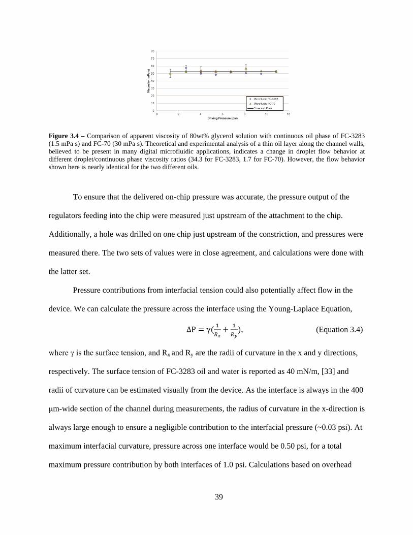
39

Figure ‎3.4 – Comparison of apparent viscosity of 80wt% glycerol solution with continuous oil phase of FC-3283

(1.5 mPa s) and FC-70 (30 mPa s). Theoretical and experimental analysis of a thin oil layer along the channel walls,

believed to be present in many digital microfluidic applications, indicates a change in droplet flow behavior at

different droplet/continuous phase viscosity ratios (34.3 for FC-3283, 1.7 for FC-70). However, the flow behavior

shown here is nearly identical for the two different oils.

To ensure that the delivered on-chip pressure was accurate, the pressure output of the

regulators feeding into the chip were measured just upstream of the attachment to the chip.

Additionally, a hole was drilled on one chip just upstream of the constriction, and pressures were

measured there. The two sets of values were in close agreement, and calculations were done with

the latter set.

Pressure contributions from interfacial tension could also potentially affect flow in the

device. We can calculate the pressure across the interface using the Young-Laplace Equation,

, (Equation 3.4)

where γ is the surface tension, and Rx and Ry are the radii of curvature in the x and y directions,

respectively. The surface tension of FC-3283 oil and water is reported as 40 mN/m, [33] and

radii of curvature can be estimated visually from the device. As the interface is always in the 400

μm-wide section of the channel during measurements, the radius of curvature in the x-direction is

always large enough to ensure a negligible contribution to the interfacial pressure (~0.03 psi). At

maximum interfacial curvature, pressure across one interface would be 0.50 psi, for a total

maximum pressure contribution by both interfaces of 1.0 psi. Calculations based on overhead

40

observation of the interface during device operation estimate a potential pressure of up to 0.30

psi at each interface, for a theoretical maximum of 0.60 psi. The contact angle, and therefore the

interface shape, may differ in channels constructed from other materials, as the channel surface

roughness would vary. Back calculation from our observed flow rates shows that a total

interfacial pressure of 0.44 psi, opposing the applied pressure, would best explain the observed

phenomenon; this pressure is well within the theoretical ranges discussed above.

Once this interfacial pressure correction is applied, the ratio of measured viscosities

becomes close to unity at all operating pressures. Data for all eight operating pressures are shown

in Figure 3.5, and the pressure-ratio trend is captured in Figure 3.6. The results produced by the

device are accurate and precise, with an average absolute value of the relative error of 6.6% ±

7.0% and an average relative standard deviation of 2.8% ± 3.7%.

41

Figure ‎3.5 – Cone-and-plate measured viscosity compared to viscosity calculated with the Hagen-Poiseuille

equation from flow in the microfluidic device, driven at a) 1.2 psi, b) 2.7 psi, c) 4.0 psi, d) 5.4 psi, e) 6.7 psi, f) 8.1

psi, g) 9.5 psi, and h) 10.9 psi, with an adjustment for interfacial pressure. All data points are the average of three

runs, with error bars representing standard deviation. The solid line is for reference and has a slope of unity. The

overall trend for operation at all pressures is shown in Figure 3.6.

42

Figure ‎3.6 – Average ratio of microfluidic viscosity to cone-and-plate viscosity for each operating pressure with an

adjustment for interfacial pressure. Average is determined by the slope of a linear best-fit line to data such as those

shown in Figure 3.5.

3.4 Conclusion

Our device offers a versatile, simple way to quickly measure the viscosity of a sample

plug, with volumes at least as small as 30 nL. The measurement requires no droplet merging or

splitting, and needs no labels, tracers, or other additives to the droplet. Measurements are

accurate and precise at all operating pressures when an interfacial backpressure is accounted for,

and accurate at higher pressures regardless.

Operation could be further automated by the inclusion of electronic droplet sensors on the

device, [34] removing the need for visual observation. Combined with the reliable operation at

high pressures, this would enable high-throughput analysis. The technique developed here is

compatible with many other microfluidic operations, and could be combined with other

procedures, including reactions or analyses. Polymerization reactions and other analyses with

significant viscosity changes would especially benefit from this technique.

43

3.5 Acknowledgements

I would like to give special thanks to Brian N. Johnson for experimental assistance and

LabVIEW programming, to Dr. Ramsey I. Zeitoun for experimental discussion, and to Leo

Pavlovsky and Prof. Michael J. Solomon for use of their rheometer. Devices were fabricated in

the Lurie Nanofabrication Facility and the Chemical Engineering Cleanroom at the University of

Michigan. This work was funded in part by NIH R01 EB006789.

44

3.6 References

1. G. M. Whitesides. What Comes Next? Lab on a Chip, 2011, 11: 191-193.

2. J. W. G. Yarnell, I. A. Baker, P. M. Sweetnam, D. Bainton, J. R. Obrien, P. J. Whitehead,

and P. C. Elwood. Fibrinogen, viscosity, and white blood cell count are major risk factors

for ischemic heart disease. The Caerphilly and Speedwell collaborative heart disease

studies. Circulation, 1991, 83(3): 836-844.

3. A. Peters, A. Döring, H. E. Wichmann, and W. Koenig. Increased plasma viscosity

during an air pollution episode: a link to mortality. Lancet, 1997, 349(9065): 1582-1587.

4. S. Shak, D. J. Capon, R. Hellmiss, S. A. Marsters, and C. L. Baker. Recombinant human

DNase I reduces the viscosity of cystic fibrosis sputum. Proceedings of the National

Academy of Sciences of the United States of America, 1990, 87(23): 9188-9192.

5. R. J. Vankooij, H. J. M. Roelofs, G. A. M. Kathmann, and M. F. Kramer. Human cervical

mucus and its mucous glycoprotein during the menstrual cycle. Fertility and Sterility,

1980, 34(3): 226-233.

6. J. Rutllant, M. Lopez-Bejar, and F. Lopez-Gatius. Ultrastructural and Rheological

Properties of Bovine Vaginal Fluid and its Relation to Sperm Motility and Fertilization: a

Review. Reproduction in Domestic Animals, 2005, 40(2): 79-86.

7. D. Mortimer, A. A. Templeton, E. A. Lenton, and R. A. Coleman. Influence of

Abstinence and Ejaculation Delay on Semen Analysis Parameters of Suspected Infertile

Men. Systems Biology in Reproductive Medicine, 1982, 8(3): 165-171.

8. P. Rosati, P. Pola, P. Riccardi, R. Flore, P. Tondi, and U. Bellati. The use of amniotic

fluid viscosity measurements to establish fetal lung maturity. International Journal of

Gynecology & Obstetrics, 1991, 35(4): 351-355.

9. G. Helms, P. Rittmann, P. Wefstaedt, H. Windhagen, T. Pressel, B. A. Behrens, and I.

Nolte. Viscosity determination of synovial fluids from the canine hip and elbow joint as

well as the human knee joint. Berliner und Münchener Tierärztliche Wochenschrift,

2008, 121(9-10): 374-380.

10. J. Jezek, M. Rides, B. Derham, J. Moore, E. Cerasoli, R. Simler, and B. Perez-Ramirez.

Viscosity of concentrated therapeutic protein compositions. Advanced Drug Delivery

Reviews, 2011, 63(13): 1107-1117.

11. M. E. M. Cromwell, E. Hilario, and F. Jacobson. Protein aggregation and bioprocessing.

AAPS Journal, 2006, 8(3): E572-E-579.

12. P. L. Evans, L. W. Schwartz, and R. V. Roy. A Mathematical Model for Crater Defect

Formation in a Drying Paint Layer. Journal of Colloid and Interface Science, 2000,

227(1): 191-205.

45

13. P. J. Cullen, A. P. Duffy, C. P. O’Donnell, and D. J. O’Callaghan. Process viscometry for

the food industry. Trends in Food Science & Technology, 2000, 11(12): 451-457.

14. H. A. Barnes. Rheology of emulsions – a review. Colloids and Surfaces A:

Physicochemical and Engineering Aspects, 1994, 91: 89-95.

15. J. M. Dealy, R. G. Larson, Structure and Rheology of Molten Polymers – From Structure

to Flow Behavior and Back Again, Hanser Publishers, 2006.

16. K. M. Schultz and E. M. Furst. High-throughput rheology in a microfluidic device. Lab

on a Chip, 2011, 11: 3802-3809.

17. N. Srivastava, R. D. Davenport, and M. A. Burns. Nanoliter viscometer for analyzing

blood plasma and other liquid samples. Analytical Chemistry, 2005, 77(2): 383-392.


capillary viscometer. Analytical Chemistry, 2006, 78(5): 1690-1696.

19. W. J. Lan, S. W. Li, J. H. Xu, and G. S. Luo. Rapid measurement of fluid viscosity using

co-flowing in a co-axial microfluidic device. Microfluidics and Nanofluidics, 2010, 8:

687-693.

20. J. Chevalier and F. Ayela. Microfluidic on chip viscometers. Review of Scientific

Instruments, 2008, 79: 076102.

21. P. Guillot, T. Moulin, R. Kötitz, M. Guirardel, A. Dodge, M. Joanicot, A. Colin, C.-H.

Bruneau, T. Colin. Towards a continuous microfluidic rheometer. Microfluidics and

Nanofluidics, 2008, 5: 619-630.

22. C. J. Pipe, T. S. Majumdar, and G. H. McKinley. High shear rate viscometry. Rheologica

Acta, 2008, 47(5-6): 621-642.

23. S. Girardo, R. Cingolani, and D. Pisignano. Microfluidic rheology of non-Newtonian

liquids. Analytical Chemistry, 2007, 79(15): 5856-5861.

24. C. J. Pipe and G. H. McKinley. Microfluidic rheometry. Mechics Research

Communications, 2009, 36(1): 110-120.

25. P. Garstecki, M. J. Fuerstman, H. A. Stone, and G. M. Whitesides. Formation of droplets

and bubbles in a microfluidic T-junction – scaling and mechanism of break-up. Lab on a

Chip, 2006, 6(3), 437-446.

26. D. Han and K.-J. Lee. Viscous dissipation in micro-channels. Journal of Mechanical

Science and Technology, 2007, 21(12): 2244-2249.

27. E. Lauga, M. P. Brenner, and H. A. Stone, in Handbook of Experimental Fluid Dynamics,

Springer, Berlin, 2007, vol. 1, ch. 19, pp. 1219-1240.

46

28. F. Jousse, G. Lian, R. Janes, and J. Melrose. Compact model for multi-phase liquid-liquid

flows in micro-fluidic devices. Lab on a Chip, 2005, 5(6): 646-656.

29. E. Lac and J. D. Sherwood. Motion of a drop along the centreline of a capillary in a

pressure-driven flow. Journal of Fluid Mechanics, 2009, 640: 27-54.

30. S. A. Vanapalli, A. G. Banpurkar, D. van den Ende, M. H. G. Duits, and F. Mugele.

Hydrodynamic resistance of single confined moving drops in rectangular microchannels.

Lab on a Chip, 2009, 9(7): 982-990.

31. C. N. Baroud, F. Gallaire and R. Dangla. Dynamics of microfluidic droplets. Lab on a

Chip, 2010, 10(16): 2032-2045.

32. S. Jakiela, S. Makulska, P. M. Korczyk and P. Garstecki. Speed of flow of individual

droplets in microfluidic channels as a function of the capillary number, volume of

droplets and contrast of viscosities. Lab on a Chip, 2011, 11(21): 3603-3608.

33. H. Boukellal, S. Selimovic, Y. Jia, G. Cristobal, and S. Fraden. Simple, robust storage of

drops and fluids in a microfluidic device. Lab on a Chip, 2009, 9(2): 331-338.


capillary viscometer. Lab on a Chip, 2006, 6(6): 744-751.

47

Chapter 4

Viscoelastic Characterization of Nanoliter Droplets in Oscillatory

Microfluidic Flow

4.1 Introduction

Viscoelastic fluids and complex fluids are most commonly studied in two types of flow:

shear and extensional. [1] Traditional geometries for shear flow include cone and plate, parallel

plate, concentric cylinders (i.e., Couette), capillary, and slit. These geometries all produce flows

with simple, steady shear. Viscoelastic fluids can be studied in these geometries by imposing an

oscillatory strain or stress (usually sinusoidal) rather than a constant one. Extensional flow, on

the other hand, involves stretching fluid elements without rotating or shearing them. Extensional

flows are commonly generated in geometries including rotating clamps, parallel plates that

accelerate apart, cross-slot flow, and flow through contractions.

The study of viscoelastic fluids in a microfluidic setting dates back at least to 1976.

Thurston tested human blood under oscillatory shear flow in brass tubes with micro- and milli-

scale diameters at frequencies up to 200 Hz. [2] Contemporary microfluidic studies of

viscoelasticity also employ oscillatory flow, [3, 4] although extensional flow through

contractions is most common. [5] Contraction flows contain both shear and elongational

components, but can nonetheless provide useful information about strongly elongational mixed

48

flows. [6] Hyperbolic contraction geometries are most common as they provide a constant

extensional rate along the centerline of the channel, and several devices have been reported. [7-

10] Models and numerical simulations have been developed for this geometry. [11, 12]

Contractions can also enable study of the interfacial deformation of droplets and viscoelastic

cells. [13] A combination of cross-slot geometry with oscillatory flow has been used to explore

both extensional and shear behavior. [14] Recently, the relationship between flow rate, relaxation

time, and the onset of elastic flow instabilities in a curved channel has been used to characterize

viscoelastic fluids. [15]

Droplets and emulsions introduce additional complication to viscoelasticity, due to the

elasticity of the liquid-liquid interface between the droplet and the continuous phase.1 Even an

emulsion of two Newtonian fluids can exhibit viscoelasticity due to this interface. Oldroyd

developed a linear viscoelastic model for a Newtonian fluid emulsion in the 1950’s. [16, 17]

More recently, Palierne extended the model to allow both phases to be viscoelastic themselves.

[18] This model predicts two behavior regimes: at low frequencies, the droplet interface

contributes strongly to the elasticity; at high frequencies, the bulk liquids contribute strongly to

the elasticity. [1] Experimental results confirm the validity of this prediction. [19]

The approach taken in this work is to use oscillatory flow to study viscoelastic fluids in

microfluidic droplets. The advantages of droplet microfluidics and this growth of this subfield

over the past several years have been well reviewed. [20-22] However, the microfluidic systems

for characterizing viscoelastic fluids discussed above all employ continuous flow, rather than

droplets. Therefore, a method compatible with liquid-liquid droplet samples would be a welcome

addition, especially as many of the applications for droplet microfluidics are biological, [22] and

many biological fluids are viscoelastic. When a material is subjected to an oscillatory strain or

49

stress with angular frequency ω, the resulting stress or strain will be in or out of phase with the

driving signal. Viscous fluids respond with phase angle δ = 90°, elastic solids respond with δ =

0°, and viscoelastic fluids lie between these two bounds. The more elastic a fluid is, the lower its

phase angle.


Device Design

The device (Figure 4.1a) contains a standard T-junction geometry for formation of

droplets or plugs (Figure 4.1b.i). The main arm of the device is connected to fluid reservoirs

containing an oil phase (FC-3283, 3M), and the side arm is connected to a fluid reservoir

containing the aqueous polyacrylamide solutions under study. The contraction downstream of the

T-junction is designed to contain the overwhelming majority of hydraulic resistance in the

device, so that a pressure applied at the inlets and outlets can be considered as applied to just the

fluid in the contraction region. Therefore, when a plug is formed and positioned in the

contraction, an oscillating pressure can be applied to it (Figure 4.1b.ii) and its response can be

observed (Figure 4.1c).

50

Figure ‎4.1 – Device design and operation.

Device Fabrication

Fabrication of the devices have been described in detail previously. [23] In brief, the

device design is fabricated as a single photomask and standard photolithography techniques are

used to transfer and deep reactive ion etch the design into a silicon wafer. Individual device dies

are diced from the wafer and bonded to parylene-coated glass microscope slides by wicking UV-

curable glue. [24] Fluidic connector tips are then epoxied to the glass slide and the device is

ready for use.

Experimental Setup

Each of three fluid reservoirs – one for each inlet or outlet on the microfluidic device –

controlled through an electronic pressure regulator (VSO-EP, Parker Hannifin) connected

through a solenoid valve (Numatech, Numatics). Fluid reservoirs are constructed from 3 mL

syringe tubes, shortened by cutting the middle section and using epoxy to reattach the two

pieces. Tubing lengths are made as short as possible and moderately rigid tubing with small inner

diameter is selected, to minimize elastic effects in the system that could delay the pressure signal

response. The microfluidic device is also located on a temperature-controlled chuck. A

51

stereoscope (SZX12, Olympus) with attached high-speed camera (TM-6710, Pulnix) is

positioned above the device and used to record the droplet interfacial motion. An LED connected

to the electrical control of one of the solenoid valves is also placed on the device in view of the

camera, to allow later synchronization of the interfacial motion with the pressure signal. Pressure

regulators and solenoid valves are controlled by LabVIEW VI and programmed to output a

sinusoidal pressure signal. The left main channel inlet and the side channel inlet apply a pressure

while the right main channel outlet solenoid is open to atmosphere, with this reversing as the sine

signal becomes negative.

Fluid Composition and Characterization

Polyacrylamide (PAA) solutions are prepared from a base solution of 75% glycerol, 1.5%

NaCl, and 23.5% water (mass basis). Concentrations of PAA were 0%; 0.05%, 0.1%, and 0.5%

of 5 MDa molecular weight PAA; and 0.1% of 18 MDa molecular weight PAA. NaCl is included

to reduce the shear rate dependence of the solution viscosity, approaching a Boger fluid. [8, 25]

Water and NaCl are added first, and vortexed until completely dissolved. Next, glycerol is added

and the solution is vortexed until there are no discernable interfaces in solution. Then, the

appropriate amount of PAA is added, and the tube is inverted several times to gently mix the

solution. The tube is then placed on a shaker table until the PAA completely dissolves, and

stored in a refrigerator to prevent degradation. Prior to testing in the microfluidic device, fluids

are characterized on a standard cone and plate rheometer (AR-1000, TA Instruments) for both

viscous and elastic material properties at 20 C. Viscosity was measured versus shear rate from 1

to 2500 s-1

, and elastic properties including phase angle were measured between 1 and 6 Hz (6.3

to 37.7 radians/second).

52

Experimental Conditions

Main channel reservoirs are filled with FC-3283 oil and the side channel reservoir is

filled with sample solution. Each reservoir is connected to the pressure control system, and the

synchronization LED is placed on the device in view of the stereoscope. Chuck temperature is

controlled to 20.00 0.01 C. Pressure is applied to form a sample solution plug in the main

channel, which is then positioned to fill the contraction, with the plug interfaces located in the

next-widest region of the main channel adjacent to the contraction. Sinusoidal oscillatory

pressure is applied to the device and video recorded for ~25 seconds. Samples are tested at

pressure maximum amplitudes of 5.4 psi and 11 psi, at frequencies from 1 to 6 Hz (6.3 to 37.7

radians/second).

Data Processing

Recordings of droplet motion are analyzed with custom MATLAB scripts. First, one

script analyzes the intensity of the LED and marks time points when the LED switches off or on.

These data are fed into a second script. In this script, for each frame, the location of the interface

is determined by optical intensity and recorded. Background noise is filtered with a median filter,

and small discontinuities are smoothed. A low-pass Butter filter is used to find the midpoint

position of the interface oscillation and the data are shifted to have this midpoint at zero. The

LED time points are then used to construct a sine wave representing the pressure signal. The

angle between the pressure signal wave and the interface oscillation wave is calculated by

δ = arccos((d ∙ p)/(|d| x |p|)), (Equation 4.1)

53

where δ is the phase angle, d is the vector for the droplet interface signal, and p is the vector for

the pressure signal. Phase angles are calibrated to results for 0% PAA base solution, as described

above, and compared.


A fluid without elasticity should have a phase angle of 90 (Figure 2a). As the pressure

crosses from positive to negative, the fluid strain reaches its maximum value and begins to

decrease. For a fluid with elasticity, the phase angle decreases from 90 (Figure 2b). The

elasticity of the fluid causes the strain to begin reversing direction before the pressure has

changed sign. If there is a delay between the indication of the pressure signal (i.e., the LED) and

the actual pressure signal, the phase angle will appear to increase from 90 (Figure 2c), as the

indication on which the calculations are based occurs before the actual pressure signal.

54

Figure ‎4.2 – Theoretical behavior of sinusoidal stress and strain signals.

A lag in the pressure signal compared to the electrical signal controlling the solenoids,

regulators, and LED is expected. This is due to the elasticity of tubing, the compressibility of air

in the system, and the actuation response time of the solenoids and electronic pressure regulators.

Therefore, a sample of base solution with 0% PAA is used to calibrate the system response. All

samples were tested in triplicate, with the average reported and the standard deviation used to

generate error bars. For this solution, the cone and plate phase angle is equal or close to an

55

inelastic 90. The difference in phase angle between the cone and plate measurement and the

microfluidic measurement at each frequency is the calibration factor (Figure 3). This approaches

0 as the frequency approaches zero, as any elastic behavior should. At higher frequencies the

lag appears to plateau around 70. This behavior is consistent between the two pressure

amplitudes used in operation.

Figure ‎4.3 – Calibration of system at different frequencies for 5.4 psi and 11 psi amplitude.

All samples were tested on a cone and plate rheometer for comparison to results from the

microfluidic device (Figure 4). As expected, phase angle begins at 90 at low frequencies, where

elastic behaviors are not strongly expressed, and decreases more as the frequency increases.

Samples with higher concentrations of polymer or higher molecular weight polymer exhibit

stronger elastic behavior, as expected. This is observed by these solutions having smaller phase

angles.

56

Figure ‎4.4 – Cone and plate rheometer measurements of phase angle.

Samples were then tested in the microfluidic device (Figure 5). For both pressure

amplitudes, at lower frequencies there is significant overlap between the results for each sample

solution, making it impossible to differentiate between them. As the frequency increases, the

behavior of the different samples begins to diverge. Again, the samples with higher

concentrations of polymer or higher molecular weight polymer have smaller phase angles,

indicating their greater elasticity.

Figure ‎4.5 – Microfluidic measurements of phase angle, at a) 5.4 psi and b) 11 psi amplitude.

57

For example, a comparison at 25 rad/s (Figure 6a) shows all samples responding similarly

to the oscillatory pressure in the microfluidic device, despite responding very differently on the

cone and plate rheometer. However, at 31rad/s (Figure 6b), and more so at 37 rad/s (Figure 6c),

samples do respond noticeably differently in the microfluidic device, and it does becomes

possible to resolve between them. The results from measurements using the higher pressure

amplitude (11 psi) show greater differentiation than the lower amplitude tests (5.4 psi). In

particular, the 11 psi tests show 45-50% of the phase angle change reported by the cone and plate

rheometer tests at these higher frequencies. The 5.4 psi tests show 27-30% of the cone and plate

measurement over the same frequencies. This behavior is summarized for all frequencies used in

Figure 6d.

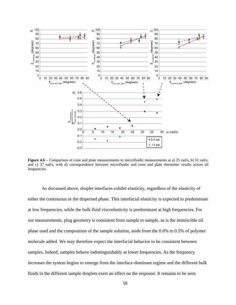
58

Figure ‎4.6 – Comparison of cone and plate measurements to microfluidic measurements at a) 25 rad/s, b) 31 rad/s,

and c) 37 rad/s, with d) correspondence between microfluidic and cone and plate rheometer results across all

frequencies.

As discussed above, droplet interfaces exhibit elasticity, regardless of the elasticity of

either the continuous or the dispersed phase. This interfacial elasticity is expected to predominate

at low frequencies, while the bulk fluid viscoelasticity is predominant at high frequencies. For

our measurements, plug geometry is consistent from sample to sample, as is the immiscible oil

phase used and the composition of the sample solution, aside from the 0.0% to 0.5% of polymer

molecule added. We may therefore expect the interfacial behavior to be consistent between

samples. Indeed, samples behave indistinguishably at lower frequencies. As the frequency

increases the system begins to emerge from the interface-dominant regime and the different bulk

fluids in the different sample droplets exert an effect on the response. It remains to be seen

59

whether these frequencies are fully into the bulk fluid-dominant regime, or still in a transitional

regime. If the latter, still higher operating frequencies may bring the microfluidic response

further in line with cone and plate results, although higher frequencies are currently beyond the

reach of our system.

4.4 Conclusion

We have presented a system for characterizing a viscoelastic microfluidic droplet based

on its phase angle. This required channel geometry is simple and compatible with upstream or

downstream droplet operations, allowing integration with droplet-based reactions, merging,

splitting, or other analysis steps. Results also offer insight into the behavior of individual droplet

interfaces. Droplet response at low frequencies is dominated by interfacial elasticity, while

sample fluid viscoelasticity becomes visible at higher frequencies. At these higher frequencies,

the response is sufficient to distinguish between different samples.

Accessing higher operating frequencies would allow further investigation of the transition

between interface-dominant and bulk fluid-dominant viscoelastic responses from microfluidic

droplets, but would likely necessitate specialized off-chip pressure control or integrated on-chip

pressure control from peristaltic or other pumps. [26] Electronic droplet sensors integrated on-

chip [27] could also further automate sample analysis. The compatibility of this technique with

other droplet-based operations opens interesting possibilities, such as observing the change in

viscoelasticity of a sample as the contents undergo a polymerization reaction, a digestion

reaction, cell growth and protein secretion, or other processes.

60

4.5 Acknowledgements

I would like to give special thanks to Brian N. Johnson for assistance with the

experimental setup and LabVIEW programming. Devices were fabricated in the Lurie

Nanofabrication Facility and the Chemical Engineering Cleanroom at the University of

Michigan.

61

4.6 References

1. R. G. Larson, The Structure and Rheology of Complex Fluids, Oxford University Press,

1999, ch. 9, pp. 409-424.

2. G. Thurston. The Effects of Frequency of Oscillatory Flow on the Impedance of Rigid,

Blood-Filled Tubes. Biorheology, 1976, 13(2): 297-301.

3. G. F. Christopher, J. M. Yoo, N. Dagalakis, S. D. Hudson, and K. B. Migler.

Development of a MEMS based dynamic rheometer. Lab on a Chip, 2010, 10(20): 2749-

2757.

4. L. Casanellas and J. Ortín. Experiments on the laminar oscillatory flow of wormlike

micellar solutions. Rheologica Acta, 2012, 51(6): 545-557.

5. F. J. Galindo-Rosales, M. A. Alves, and M. S. N. Oliveira. Microdevices for extensional

rheometry of low viscosity elastic liquids: a review. Microfluidics and Nanofluidics,

2012, 14(1-2): 1-19.

6. C. J. Pipe and G. H. McKinley. Microfluidic rheometry. Mechanics Research

Communications, 2009, 36(1): 110-120.

7. M. Chellamuthu, E. M. Arndt, and J. P. Rothstein. Extensional rheology of shear-

thickening nanoparticle suspensions. Soft Matter, 2009, 5(10): 2117-2124.

8. P. C. Sousa, P. M. Coelho, M. S. N. Oliveira, and M. A. Alves. Three-dimensional flow

of Newtonian and Boger fluids in square-square contractions. Journal of Non-Newtonian

Fluid Mechanics, 2011, 160(2-3): 122-139.

9. L. Campo-Deaño, F. J. Galindo-Rosales, F. T. Pinho, M. A. Alves, and M. S. N. Oliveira.

Flow of low viscosity Boger fluids through a microfluidic hyperbolic contraction.

Journal of Non-Newtonian Fluid Mechanics, 2011, 166(21-22): 1286-1296.

10. T. J. Ober, S. J. Haward, C. J. Pipe, J. Soulages, and G. H. McKinley. Microfluidic

extensional rheometry using a hyperbolic contraction geometry. Rheologica Acta, 2013,

52(6): 529-546.

11. M. A. Moyers-Gonzalez, R. G. Owens, and J. Fang. On the high frequency oscillatory

tube flow of healthy human blood. Journal of Non-Newtonian Fluid Mechanics, 2009,

163(1-3): 45-61.

12. M. Nyström, H. R. Tamaddon Jahromi, M. Stading, and M. F. Webster. Numerical

simulations of Boger fluids through different contraction configurations for the

development of a measuring system for extensional viscosity. Rheologica Acta, 2012,

51(8): 713-727.

62

13. J. D. Martin, J. N. Marhefka, K. B. Migler, S. D. Hudson. Interfacial Rheology Through

Microfluidics. Advanced Materials, 2011, 23(3): 426-432.

14. S. J. Haward, J. A. Odell, Z. Li, and X.-F. Yuan. Extensional rheology of dilute polymer

solutions in oscillatory cross-slot flow: the transient behavior of birefringent strands.

Rheologica Acta, 2010, 49(6): 633-645.

15. J. Zilz, C. Schäfer, C. Wagner, R. J. Poole, M. A. Alves, and A. Linder. Serpentine

channels: micro-rheometers for fluid relaxation times. Lab on a Chip, 2013, DOI:

10.1039/C3LC50809A.

16. J. G. Oldroyd. The elastic and viscous properties of emulsions and suspensions.

Proceedings of the Royal Society A: Mathematical, Physical and Engineering Sciences,

1953, 218(1132): 122-132.

17. J. G. Oldroyd. The effect of interfacial stabilizing films on the elastic and viscous

properties of emulsions. Proceedings of the Royal Society A: Mathematical, Physical and

Engineering Sciences, 1955, 232(1191): 567-577.

18. J. F. Palierne. Linear rheology of viscoelastic emulsions with interfacial tension.

Rheologica Acta, 1990, 29(3): 204-214.

19. S. Kitade, A. Ichikawa, N. Imura, Y. Takahashi, and I. Noda. Rheological properties and

domain structures of immiscible polymer blends under steady and oscillatory shear flows.

Journal of Rheology, 1997, 41(5): 1039-1060.

20. S.-Y. Teh, R. Lin, L. Hung, and A. P. Lee. Droplet microfluidics. Lab on a Chip, 2008,

8(2): 198-220.

21. R. Seemann, M. Brinkmann, T. Pfohl, and S. Herminghaus. Droplet based microfluidics.

Reports on Progress in Physics, 2012, 75(1): 016601.

22. T. Schneider, J. Kreutz, and D. Chiu. The Potential Impact of Droplet Microfluidics in

Biology. Analytical Chemistry, 2013, 85: 3476-3482.

23. E. Livak-Dahl, J. Lee, and M. A. Burns. Nanoliter droplet viscometer with additive-free

operation. Lab on a Chip, 2013, 13(2): 297-301.

24. S. M. Langelier, L. Y. Yeo, and J. Friend. UV epoxy bonding for enhanced SAW

transmission and microscale acoustofluidic integration. Lab on a Chip, 2012, 12(16):

2970-2976.

25. D. F. James. Boger Fluids. Annual Review of Fluid Mechanics, 2009, 41(1): 129-142.

26. M. A. Unger, H. P. Chou, T. Thorsen, A. Scherer, and S. R. Quake. Monolithic

microfabricated valves and pumps by multilayer soft lithography. Science, 2000,

288(5463): 113-116.

63

27. N. Srivastava and M. A. Burns. Electronic drop sensing in microfluidic devices:

automated operation of a nanoliter viscometer. Lab on a Chip, 2006, 6(6): 744-751.

64

Chapter 5

Preliminary Design, Fabrication, and Testing of Plasma-Based

Microscale Pressure Actuator

5.1 Introduction

Micro-Scale Flow Control

The most straightforward way to generate flows in a microfluidic device is with external

(“off-chip”) pressure sources, either as a constant pressure source or a constant volumetric flow

rate (e.g. a syringe pump). This approach results in simpler device designs and easier fabrication

processes, and can be used for both continuous media [1] and discrete droplets. [2] However, use

of external pressure sources makes harder the precise control and positioning of droplets, due to

the subtle pressure differences needed. Additionally, reliance on external pressure sources

greatly reduces the portability of microfluidic devices, an important concern especially for

devices aimed at on-site medical diagnostics or other field testing applications.

There are also many “on-chip” methods for flow control. Conceptually, the most

straightforward is the micropump. There are several designs for on-chip pumps, primarily either

reciprocating displacement pumps or peristaltic pumps. Akin to a traditional piston pump,

reciprocating displacement micropumps use diaphragms connected with a rectifier to generate

net fluidic displacement in one direction. [3, 4] Alternatively, valves with off-chip actuation or

65

diaphragms can be combined in series to form peristaltic pumps. [5] These displacement pumps

are mechanically complicated, and their fabrication procedures are complex and costly. Valve-

based peristaltic pumps still require off-chip pumping equipment, and so their portability is

limited.

Electroosmotic flow (EOF) was first developed for flow control in capillary

electrophoresis (CE). CE first arose in the early-to-mid-1980’s as a separation technique

complementary to gel-based electrophoresis and high-performance liquid chromatography

(HPLC) and was used for separating electrolytes in solution. [6, 7] The phenomenon of

electroosmosis arises from the electrolytes in solution equilibrating with the surrounding channel

walls, forming an ionic double layer – the Debye layer – near the solid-liquid interface. An

applied electric field then causes this layer to migrate, resulting in bulk flow throughout the

capillary. The technique, originally developed in glass capillaries, can be successfully applied in

PDMS, silicon or glass microchannels through the continuous application and manipulation of

voltages. [8] In addition to ease of control, the other major attraction of EOF is that fluid velocity

is not hindered by decreasing the channel dimensions. However, only conductive fluids can be

pumped, limiting the application of EOF.

Another technique prominent at the microscale is the use of surfaces forces to control

flow. Because of the increased surface area-to-volume ratio, interfacial interactions between the

fluid and the channel walls can be used to pump fluids through the device. [9]Alternatively,

capillary pressure-driven flows can be actively controlled by using heat, [10] or more commonly,

electrical fields (known as electrowetting on dielectric – EWOD) [11] to alter the contact angle

between the fluid and the surface. These techniques require a high degree of thermal or electrical

66

control, however, and therefore require thermal isolation on-chip or a large number of electrodes

across the device, respectively.

A more recent area of study for microfluidic flow control is acoustics. Generating high-

amplitude acoustic waves with a piezoelectric actuator, acoustic streaming devices exert a

directed body force on the fluid in the direction of the wave via acoustic attenuation. [12] These

actuators can pump or mix bulk fluid in channels. Droplets on surfaces can also be controlled by

acoustic streaming. A surface acoustic wave (SAW) is generated on a piezoelectric substrate and

causes acoustic streaming as its energy is dissipated within the droplet, [13] and this causes the

droplet to roll across the surface in a controlled manner. These acoustic approaches seem to hold

much promise for microfluidic flow control, and while they do necessitate the use of

piezoelectric substrates, the field bears more investigation.

Plasma-Based Flow Actuation

In the past decade or so, aeronautic researchers have developed plasma actuators for

electrohydrodynamic (EHD) flow control in room temperature atmospheric air. [14-16] Their

goal is to achieve flow control in boundary layers and over airfoils to prevent or cause boundary

layer separation, to reduce drag and enhance lift, and to stabilize or mix airflow to dampen

vibrations. [17] Most work so far involves dielectric barrier discharge (DBD) plasmas, which

were first studied in 1857 by Ernst Werner von Siemens and have many applications, including

ozone production for air and water treatment, high-power CO2 lasers, and flat panel plasma

displays. [18] DBD generators consist of a pair of electrodes separated by a dielectric with one

connected to ground. A radio frequency AC voltage (several thousand volts and several to tens of

kHz) is applied to the other electrode.

67

Aeronautical plasma actuators use a planar DBD design rather than the volumetric design

more common in industrial processes. In this design, the grounded electrode is covered by a

dielectric and the powered electrode is exposed to the air. When powered, this configuration

generates plasma downstream of the exposed electrode which imparts a force on the surrounding

neutral air in the direction of the covered electrode. [19] This force can generate airflows of

several meters per second; these airflows are commonly called “electric wind” or “ionic wind.”

These DBD actuators are attractive because they can operate in air at atmospheric

pressure rather than vacuum, room temperature rather than high temperature, and can be

powered by a standard sine waveform voltage rather than a sophisticated pulsed power supply.

[17] Electrodes are usually a few millimeters wide, and typical dielectric materials are Teflon,

Kapton, glass, ceramic, and Plexiglass, with a thickness of 0.1 to a few millimeters. Current

work in the field focuses mainly on numerical simulations of the plasma [20] and increasing

power efficiency. [21]

The breakdown voltage for an electric discharge in a gas is empirically described by

Paschen’s law,

, (Equation 5.1)

where V is the breakdown voltage, p is the pressure, and d is the gap distance. The constants a

and b are dependent on the gas composition, and Paschen’s law curves for several gases are

shown in Figure 5.1. All curves have the same overall shape, where a minimum voltage is

reached as pd decreases. Below this minimum, the breakdown voltage drastically increases, as

there are fewer and fewer molecules within between the electrodes to conduct the current.

68

Figure ‎5.1 – Paschen’s law curves for helium, neon, argon, hydrogen, and nitrogen. Graph by Gianluca Spizzo,

using data from [22].

Aerodynamic plasma actuators have been confirmed to use dielectric barrier discharge

(DBD) plasmas, as initially suspected. [23] The most important characteristic of such plasmas is

their ability to sustain large-volume discharges without collapsing into an arc. This is due to the

self-limiting nature of the actuator configuration. In the half of the AC cycle where the exposed

electrode is more negative than the insulated electrode and so acts as the cathode in the

discharge. As the magnitude of the applied negative voltage increases, the exposed electrode can

discharge electrons; at the same time, charge builds up on the dielectric surface. Once the

69

magnitude of the negative voltage begins to decrease, however, the built up charge on dielectric

is sufficient to oppose the applied voltage and the discharge shuts off. As the applied voltage

becomes more positive, the charge on the dielectric now acts as the cathode and the plasma can

reignite in the opposite direction. However, the charge supply is limited to that already present

on the dielectric. Once the magnitude of the positive voltage begins to decrease, the discharge

shuts off again, as in the first half-cycle. The plasma discharge, while appearing continuous to

the eye, is in fact temporally structured. [23]

The ions and electrons generated by the plasma collide with neutral particles in the region

between the two electrodes, generating the phenomenon known as electric wind or ionic wind,

first reported in 1709. [17] Due to their much lower mass, electron contribution to electric wind

can be ignored, and the neutral gas velocity generated can be described by Equation 5.2,

G

G

idv

A , (Equation 5.2)

where i is the time-averaged discharge current, d is the electrode gap, is the gas density, is

the ion mobility, and AG is the discharge cross-section. Alternatively, Roth [24] relates the

electrostatic pressure, pE, generated by the plasma to the dynamic, or stagnation, pressure, ps, of

the neutral gas flowing away from the plasma,

2 2

0

1 1

2 2s G Ep v E p , (Equation 5.3)

and solves for the velocity in terms of the electrical field,

0Gv E

, (Equation 5.4)

where 0 is the permittivity of free space and E is the electric field strength.

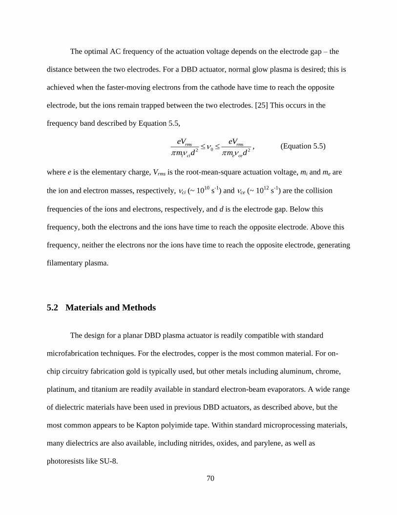
70

The optimal AC frequency of the actuation voltage depends on the electrode gap – the

distance between the two electrodes. For a DBD actuator, normal glow plasma is desired; this is

achieved when the faster-moving electrons from the cathode have time to reach the opposite

electrode, but the ions remain trapped between the two electrodes. [25] This occurs in the

frequency band described by Equation 5.5,

02 2

rms rms

i ci e ce

eV eV

m d m d

, (Equation 5.5)

where e is the elementary charge, Vrms is the root-mean-square actuation voltage, mi and me are

the ion and electron masses, respectively, ci (~ 1010

s-1

) and ce (~ 1012

s-1

) are the collision

frequencies of the ions and electrons, respectively, and d is the electrode gap. Below this

frequency, both the electrons and the ions have time to reach the opposite electrode. Above this

frequency, neither the electrons nor the ions have time to reach the opposite electrode, generating

filamentary plasma.


The design for a planar DBD plasma actuator is readily compatible with standard

microfabrication techniques. For the electrodes, copper is the most common material. For on-

chip circuitry fabrication gold is typically used, but other metals including aluminum, chrome,

platinum, and titanium are readily available in standard electron-beam evaporators. A wide range

of dielectric materials have been used in previous DBD actuators, as described above, but the

most common appears to be Kapton polyimide tape. Within standard microprocessing materials,

many dielectrics are also available, including nitrides, oxides, and parylene, as well as

photoresists like SU-8.

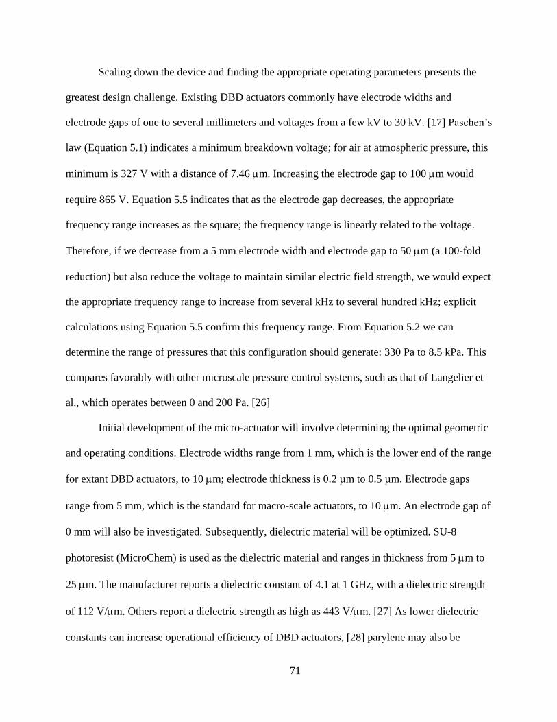
71

Scaling down the device and finding the appropriate operating parameters presents the

greatest design challenge. Existing DBD actuators commonly have electrode widths and

electrode gaps of one to several millimeters and voltages from a few kV to 30 kV. [17] Paschen’s

law (Equation 5.1) indicates a minimum breakdown voltage; for air at atmospheric pressure, this

minimum is 327 V with a distance of 7.46 m. Increasing the electrode gap to 100 m would

require 865 V. Equation 5.5 indicates that as the electrode gap decreases, the appropriate

frequency range increases as the square; the frequency range is linearly related to the voltage.

Therefore, if we decrease from a 5 mm electrode width and electrode gap to 50 m (a 100-fold

reduction) but also reduce the voltage to maintain similar electric field strength, we would expect

the appropriate frequency range to increase from several kHz to several hundred kHz; explicit

calculations using Equation 5.5 confirm this frequency range. From Equation 5.2 we can

determine the range of pressures that this configuration should generate: 330 Pa to 8.5 kPa. This

compares favorably with other microscale pressure control systems, such as that of Langelier et

al., which operates between 0 and 200 Pa. [26]

Initial development of the micro-actuator will involve determining the optimal geometric

and operating conditions. Electrode widths range from 1 mm, which is the lower end of the range

for extant DBD actuators, to 10 m; electrode thickness is 0.2 µm to 0.5 µm. Electrode gaps

range from 5 mm, which is the standard for macro-scale actuators, to 10 m. An electrode gap of

0 mm will also be investigated. Subsequently, dielectric material will be optimized. SU-8

photoresist (MicroChem) is used as the dielectric material and ranges in thickness from 5 m to

25 m. The manufacturer reports a dielectric constant of 4.1 at 1 GHz, with a dielectric strength

of 112 V/m. Others report a dielectric strength as high as 443 V/m. [27] As lower dielectric

constants can increase operational efficiency of DBD actuators, [28] parylene may also be

72

investigated as a dielectric material. Appropriate voltage ranges to maintain similar electric field

strength are used as described above, remaining in the tens of kV/cm. Voltage losses across the

system, as well as the frequency dependence of the impedance, are unknown, and will be

optimized for empirically.

Fabrication is performed by standard photolithography techniques. The design for the

grounded electrodes is patterned onto SPR220 photoresist, spin-coated to a thickness of 3 m on

a glass wafer. Chrome and gold are deposited and patterned by lift-off removal of the photoresist

layer. The dielectric layer of SU-8 is spin-coated on top of the electrodes, exposed, and baked.

Finally, the upper electrode layer is fabricated by the same procedure, with the design being

aligned to the lower layer.


Initial testing at 10 kHz resulted in plasma discharge along the length of the electrodes, at

voltages from 2200 V to 2400 V. This discharge persisted for ~15 seconds before dielectric

breakdown rendered the actuator unusable. The aftermath of the discharge is visible in Figure 5.2

as the brightly colored horizontal regions between the two electrodes.

73

Figure ‎5.2 – Dielectric breakdown following operation of plasma actuators. Actuators operated for ~15 seconds at

10 kHz and 2200 to 2400 V, producing a plasma discharge along the length of the electrodes. Bright regions indicate

damaged SU-8.

After relocation of the high voltage test setup to our lab, this behavior could not be

replicated. Operation was conducted under the same conditions with electrodes from the same

fabrication batch. However, rather than a plasma discharge along the length of the electrodes, the

only observed behavior was arcing from the connection pads and leads of the grounded electrode

to the body of the upper exposed electrode. This resulted in the destruction of regions, or in some

cases the entirety, of the upper electrode. Efforts made to insulate the connections, prevent this

behavior, and restore the plasma discharge were unsuccessful.

5.4 Conclusion

This work has much potential, but we lack the expertise to sufficiently diagnose the

problems with the current configuration. Plasma physics and high voltage, high frequency

74

electronics are beyond the normal scope of our group’s research. Resources and time did not

allow for sufficient cultivation of collaborations with other researchers who might provide the

necessary knowledge. Recently, micron-scale dielectric barrier discharge plasma-based pressure

actuators have been reported, [29] although their application to microfluidics settings remains to

be demonstrated.

75

5.5 References

1. B. Zheng, J. D. Tice, R. F. Ismagilov. Formation of droplets of alternating composition

in microfluidic channels and applications to indexing of concentrations in droplet-based

assays. Analytical Chemistry, 2004, 76(17): 4977-4982.

2. R. Pal, M. Yang, R. Lin, B. N. Johnson, N. Srivastava, S. Z. Razzacki, K. J. Chomistek,

D. C. Heldsinger, R. M. Haque, V. M. Ugaz, P. K. Thwar, Z. Chen, K. Alfano, M. B.

Yim, M. Krishnan, A. O. Fuller, R. G. Larson, D. T. Burke, and M. A. Burns. An

integrated microfluidic device for influenza and other genetic analyses. Lab on a Chip,

2005, 5(10): 1024-1032.

3. A. Olsson, P. Enoksson, G. Stemme, and E. Stemme. Micromachined flat-walled

valveless diffuser pumps. Journal of Microelectromechanical Systems, 1997, 6(2): 161-

166.

4. D. J. Laser and J. G. Santiago. A review of micropumps. Journal of Micromechanics and

Microengineering, 2004, 14(6): R35-R64.

5. M. A. Unger, H.-P. Chou, T. Thorsen, A. Scherer, and S. R. Quake. Monolithic

microfabricated valves and pumps by multilayer soft lithography. Science, 2000,

288(5463): 113-116.

6. J. W. Jorgenson and K. Lukacs. Capillary zone electrophoresis. Science, 1983,

222(4621): 266-272.

7. X. Huang, M. J. Gordon, and R. N. Zare. Current-monitoring method for measuring the

electroosmotic flow rate in capillary zone electrophoresis. Analytical Chemistry, 1988,

60(17): 1837-1838.

8. G. Ocvirk, M. Munroe, T. Tang, R. Oleschuk, K. Westra, and D. J. Harrison.

Electrokinetic control of fluid flow in native poly(dimethylsiloxane) capillary

electrophoresis devices. Electrophoresis, 2000, 21(1): 107-115.

9. D. Juncker, H. Schmid, U. Drechsler, H. Wolf, M. Wolf, B. Michel, N. de Rooij, and E.

Delamarche. Autonomous microfluidic capillary system. Analytical Chemistry, 2002,

74(24): 6139-6144.

10. T. S. Sammarco and M. A. Burns. Thermocapillary pumping of discrete drops in

microfabricated analysis devices. Journal of the American Institute of Chemical

Engineers, 1999, 45(2): 350-366.

11. S. K. Cho, H. Moon, and C.-J. Kim. Creating, transporting, cutting, and merging liquid

droplets by electrowetting-based actuation for digital microfluidic circuits. Journal of

Microelectromechanical Systems, 2003, 12(1): 70-80.

76

12. J. C. Rife, M. I. Bell, J. S. Horwitz, M. N. Kabler, R. C. Y. Auyeung, and W. J. Kim.

Miniature valveless ultrasonic pumps and mixers. Sensors and Actuators A: Physical,

2000, 86(1-2): 135-140.

13. A. Wixforth. Acoustically driven planar microfluidics. Superlattices and Superstructures,

2003, 33(5-6): 389-396.

14. J. Roth, D. Sherman, and S. Wilkinson. Electrohydrodynamic flow control with a glow-

discharge surface plasma. AIAA Journal, 2000, 38(7): 1166-1172.

15. T. C. Corke, C. L. Enloe, and S. P. Wilkinson. Dielectric Barrier Discharge Plasma

Actuators for Flow Control. Annual Review of Fluid Mechanics, 2010, 42: 505-529.

16. L. N. Cattafesta III and M. Sheplak. Actuators for Active Flow Control. Annual Review

of Fluid Mechanics, 2011, 43: 247-272.

17. E. Moreau. Airflow control by non-thermal plasma actuators. Journal of Physics D:

Applied Physics, 2007, 40(3): 605-636.

18. U. Kogelschatz, B. Eliasson, and W. Egli. From ozone generators to flat television

screens: history and future potential of dielectric barrier discharges. Pure and Applied

Chemistry, 1999, 71(10): 1819-1828.

19. G. I. Font and W. L. Morgan. Recent progress in dielectric barrier discharges for

aerodynamic flow control. Contributions to Plasma Physics, 2007, 47(1-2): 103-110.

20. E. Peers, Z. Ma, and X. Huang. A numerical model of plasma effects in flow control.

Physics Letters A, 2010, 374(13-14): 1501-1504.

21. J.-H. Kim, M. Nishihara, I. V. Adamovich, M. Samimy, S. V. Gorbatov, and F. V.

Pliavaka. Development of localized arc filament RF plasma actuators for high-speed and

high Reynolds number flow control. Experiements in Fluids, 2010, 49(2): 497-511.

22. Lieberman and Lichtenberg, Principles of Plasma Discharges, Wiley, 2005.

23. C. L. Enloe, T. E. McLaughlin, R. D. VanDyken, K. D. Kachner, E. J. Jumper, and T. C.

Corke. Mechanisms and responses of a single dielectric barrier plasma actuator: plasma

morphology. AIAA Journal, 2004, 42(3): 589-594.

24. J. Roth. Aerodynamic flow acceleration using paraelectric and peristaltic

electrohydrodynamic effects of a One Atmosphere Uniform Glow Discharge Plasma.

Physics of Plasmas, 2003, 10(5): 2117-2126.

25. D. S. Chang. Compressible Flows for Fluidic Control in Microdevices; University of

Michigan: Ann Arbor, MI, 2010.

77

26. S. M. Langelier, D. S. Chang, R. I. Zeitoun, and M. A. Burns. Acoustically driven

programmable liquid motion using resonance cavities. Proceedings of the National

Academy of Sciences of United States of America, 2009, 106(31): 12617-12622.

27. J. Melai, C. Salm, S. Smits, J. Visschers, and J. Schmitz. The electrical conduction and

dielectric strength of SU-8. Journal of Micromechanics and Microengineering, 2009, 19:

065012.

28. M. Forte, J. Jolibois, J. Pons, E. Moreau, G. Touchard, and M. Cazalens. Optimization of

a dielectric barrier discharge actuator by stationary and non-stationary measurements of

the induced flow velocity: application to airflow control. Experiments in Fluids, 2007,

43(6): 917-928.

29. J. C. Zito, R. J. Durscher, J. Soni, S. Roy, and D. P. Arnold. Flow and force inducement

using micron size dielectric barrier discharge actuators. Applied Physics Letters, 2012,

100(19): 193502.

78

Chapter 6

Single-Mask 3D Microchannel Mold Fabrication by SU-8

Release and Reattachment

6.1 Introduction

The development of microfluidic devices grew from the techniques pioneered in

microelectronics industry. For many applications, these techniques are more than sufficient for

the construction of channels, reactors, and separators needed in microfluidic systems.

Nonetheless, standard photolithography techniques have a major limitation in that they only

allow planar structures to be fabricated. For example, channel features in the plane of the

substrate can have arbitrary shape, but channel heights are restricted to a uniform height

perpendicular to the substrate. Access to more variability in this third dimension would allow a

wide range of microfluidic devices with more complex designs to be produced. For example, 3D

structures can enhance mixing, weirs of different heights can trap particles based on size, and

cantilevers or needles can be used in many sensing and other MEMS applications. [1]

Microfluidics researchers have worked to add complexity in the third dimension. Mosher

et al. [2] identify three primary types of 3D photolithography: multiple-step, direct write, and

gray scale. These techniques are still fundamentally planar but use either multiple exposures or

multiple exposure levels to create planar features with different heights. Multiple step

79

photolithography uses several standard optical masks, either using each mask to produce a

different exposure level in the photoresist or using each mask to expose a newly spin-coated

photoresist layer of the desired thickness. With this approach, n masks can produce n + 1

different levels. [2] However, each mask must be aligned and exposed separately, introducing

time expense and error to the process. Direct write techniques use beam- or DLP-based systems

to expose the photoresist without a mask. [1] These systems are powerful, but exposure of an

entire wafer can take hours, and the equipment is expensive. Grayscale masks produce different

exposure levels by allowing varying levels of light transmission across the mask, rather than

features being either completely transparent or completely opaque. [3] These masks are most

commonly produced by continuous tone printing or by using pixelated arrays; reconfigurable

microfluidics-based masks have also been reported. [4] Continuous tone mask printing is similar

to color printing, with different colors or gray tones having different UV absorptions. [5] Color

printing at the resolutions required for microfabrication is expensive. Pixelated grayscale masks

are comprised of micro-arrays of transparent pixels; different exposure levels are achieved by

different ratios of transparent pixel to opaque background. This approach is cheaper, but has a

lower vertical resolution than continuous tone. Combining grayscale techniques with multiple

step photolithography can improve vertical resolution by yielding 2n exposure levels, but this still

requires the production and alignment of multiple masks. Additionally, real, non-planar, 3D

structures can be fabricated in SU-8 with sub-diffraction limit resolution by using two-photon

absorption (TPA) fabrication techniques. [6] However, this approach is complex and requires

expensive equipment, as well as being far beyond the needs of most microfluidics users.

We present an approach involving the removal and reattachment of SU-8 structures to

create molds with 3D topography using a single photomask. The basic principle of creating SU-8

80

structures and releasing them from their substrate has been demonstrated, [7, 8] primarily for the

creation of SU-8 cantilevers. [9-11] In short, a structure like a cantilever is difficult to construct

by standard photolithography when oriented rightside-up, but easy to create upside-down.

Therefore, structures are fabricated upside-down, released from the substrate, reoriented, and

reattached to the substrate in their desired configuration. Here we extend this technique to the

creation of a range of SU-8 molds for PDMS channels.


Fabrication of 3D SU-8 molds and PDMS devices

Fabrication of the 3D SU-8 molds begins with the creation of SU-8 blocks by standard

photolithography techniques. SU-8 (MicroChem) is spin-coated on a bare 4-inch glass wafer

(Precision Glass and Optics); the thickness of the SU-8 layer in this step will be the width of the

eventual PDMS channel. A photomask (Fineline Imaging) is used to expose a pattern of an SU-8

block (Figure 6.1a). One long edge of the block has the desired shape or topography of the

eventual PDMS channel ceiling, and the other long edge of the block is flat, which will

subsequently be bonded to a mold substrate. After patterning and baking, the SU-8 is developed;

exposure, baking, and developing parameters are according to manufacturer recommendations. If

the SU-8 block did not detach from the glass wafer during developing, it is now removed from

the wafer with tweezers, or by hydrofluoric acid undercutting of the glass wafer if necessary

(Figure 6.1b).

81

Figure ‎6.1 – Fabrication of 3D SU-8 molds. a) SU-8 blocks are fabricated by standard methods. Blocks have one

long edge flat and one long edge with the desired topography. b) SU-8 blocks are removed from the wafer with

tweezers, or by HF acid undercutting of the wafer if necessary. c) The SU-8 blocks are manually rotated so the

desired topography is on the top face and the flat edge is on the bottom face. A thin layer of SU-8 is spun on a new

substrate. d) The block is placed on the freshly spun SU-8, which is subsequently baked, exposed, and post-

processed as normal.

A thin layer of SU-8 is spin-coated on a bare 4-inch silicon wafer (Silicon Valley

Microelectronics); 1 to 3 μm was found to be sufficient. The SU-8 block is manually rotated so

the desired topography is on the top face and the flat edge is on the bottom face (Figure 6.1c).

The rotated block is placed on the freshly spun SU-8, which is subsequently pre-baked, exposed

to UV light without a mask, and post-baked to solidify the attachment of the SU-8 block. The

mold is treated with O2 plasma from a corona treater (BD-20, Electro-Technic Products) and

exposed to tridecafluoro-1,1,2,2,-tetrahydrooctyl-1-trichlorosilane in a vacuum chamber for one

hour (Figure 6.1d) to promote PDMS release. Note that, depending on channel dimensions,

hundreds of blocks can be fabricated on one glass wafer, and dozens can fit on one silicon wafer

mold.

PDMS (Sylgard 184, Dow Corning) is mixed in a 10:1 monomer:crosslinker ratio and

poured over the prepared 3D SU-8 mold. The mold is then placed under vacuum for 30-60

82

minutes to remove all bubbles, and then baked at atmospheric pressure for 1-2 hours at ~80 °C.

After cooling to room temperature, the PDMS is carefully peeled from the mold and cut into

individual devices with a razor. A biopsy punch is used to create access holes at the entrance and

exit of the 3D PDMS channel. Glass slides are cleaned with piranha solution, PDMS devices are

cleaned with Scotch tape (3M), and the two are treated with O2 plasma for ~30 seconds before

being placed in contact. The bond is allowed to strengthen for ~1 hour on a hot plate at 70 °C.

Particle experiments

All particle-based experiments use fluorescent polystyrene (~20 μm and ~30 μm

diameter) and PMMA (~40 μm diameter) particles in yellow, purple and Nile red (Spherotech).

Particle solutions used in experiments contain only concentrated particle solution and DI water,

and were vortexed for one minute immediately before use to ensure mixing. Experiments are

conducted in PDMS devices fabricated as described above. Particle solutions are pulled through

the device from a syringe reservoir by an electronic vacuum regulator (VSO-EV, Parker

Hannifin) controlled via LabVIEW software (National Instruments). Devices are viewed with a

fluorescent microscope (Eclipse Ti-S, Nikon) and images captured via digital camera (EXi Blue,

QImaging). For the saw tooth particle organization experiment, the PDMS channel was

incubated with a 1% solution of bovine serum albumin (Sigma-Aldrich) for two hours prior to

the experiment to reduce particle adhesion, and subsequently degassed in a vacuum chamber for

1 hour to reduce bubble formation.

83


A wide range of SU-8 mold shapes can be produced (Figure 6.2), including gradual

slopes (Figure 6.2a) and saw tooth structures (Figure 6.2b). Note that these features have smooth

edges and do not have the step-changes in height found with multi-mask and some grayscale

fabrication methods. Overhanging features, such as a modified saw tooth shape with 45° angles

(Figure 6.2c) are also easily created. While features with significant overhangs are not suitable

for casting and release of PDMS, sloped overhangs like those shown here are capable of

releasing PDMS without breaking. Molds for channels with different height regions are also

possible, such as a larger diameter flow region and an increasingly narrow particle-trapping

region (Figure 6.2d). 3D mold structures formed by this technique are close to perpendicular

with the wafer, despite being positioned manually (Figure 6.3). Average deviation from

perpendicular (90°) is 2.8° ± 3.0°.

This technique provides easy fabrication of channels with changing flow characteristics.

For example, particles can be self-organized on channel surfaces with guiding features. Particles

were shown to organize in a PDMS channel with saw tooth topography cast from the mold

shown in Figure 2b. After the channel was fabricated and prepared as described previously, a

solution of fluorescent 40 μm diameter PMMA particles was injected into the channel with the

channel oriented so the saw tooth topography was the channel roof (Figure 6.4a). The channel

was then flipped upside down and immediately imaged again (Figure 6.4b). The high density

(i.e., higher than water) of PMMA (1.18 g/cm3) causes the particles to settle through the solution

and self-organize into rows on the saw tooth valleys on the channel floor.

84

Figure ‎6.2 – Microscopy images (upper) and line drawings (lower) of various 3D channel molds. a) Long gradual

slope. b) Triangle wave (see Fig. 6.4). c) Modified saw tooth wave, at heights from 5 to 50 μm, with 45° overhang.

d) Channel with particle trapping region, with height decreasing from 50 μm to 15 μm (see Fig. 6.6).

Figure ‎6.3 – Angle between bottom and channel wall for PDMS devices cast from 3D SU-8 block molds. Average

deviation from vertical (90°) is 2.8° ± 3.0° (n = 17 channels measured).

85

Figure ‎6.4 – Fluorescent microscope image of particle organization in saw tooth PDMS device cast from mold

shown in Fig. 2b. a) 40 μm-diameter PMMA particles are flowed into a channel with a saw tooth-shaped roof. b)

The device is inverted and the particles organize into rows as they settle on the saw tooth-shaped floor.

Particles were also shown to come into focus for microscope imaging in a PDMS channel

with varying height. The channel was cast from a mold similar to that shown in Figure 6.2d, but

with a constant 50-μm height in the center region. The shorter channel height in the center region

forces the particles (20 μm fluorescent polystyrene) into the focal plane of the microscope, while

particles in the taller regions upstream and downstream are either in or out of focus (Figure 6.5).

The center in-focus region allows imaging of all particles, while the taller regions reduce the

hydrodynamic resistance of the channel and allow for faster flow rates at a given pressure. The

gradual slope down to the center region ensures particles are not trapped in dead zones. Note

that the particle velocity can be increased or decreased by decreasing or increasing the channel

height, respectively.

Figure ‎6.5 – Fluorescent microscope image of particle imaging device. Mold design is similar to Fig. 2d, but with

constant 50 μm channel height in center region. The taller main channel affords lower hydrodynamic resistance,

while the center region brings particles into the focal plane of the microscope for imaging. Particles are 20 μm in

diameter

86

.

Particles can also be sorted based on size and trapped in a PDMS channel with a gradual

height change. A channel was cast from the mold shown in Figure 6.2d. Particles of varying

diameters (20 μm, 30 μm, and 40 μm), each size particle fluorescent at a different wavelength,

were injected into a channel with the height decreasing from 50 μm to 15 μm. Moving

downstream, the larger particles get trapped against the lowering channel roof followed by the

progressively smaller particles (Figure 6.6). The fact that the channel narrows vertically more

readily allows smaller particles to move around larger particles already trapped upstream, rather

than simply jamming behind them and clogging. Additionally, this configuration allows

visualization of the trapped particles that would not be possible if the channel trapped particles

by narrowing horizontally, and allows a simple calculation of particle size dispersity.

Figure ‎6.6 – Fluorescent microscope composite image of size-based particle separation in a PDMS device cast from

an SU-8 mold similar to that shown in Fig. 2d. Channel height changes from 50 μm at the left of the image to 15 μm

at the right. Fluorescent particles of different sizes and colors were mixed together and flowed through the device.

As the channel height decreases, larger particles become stuck earlier than smaller particles.

6.4 Conclusions

The technique we have demonstrated allows the creation of SU-8 molds for linear PDMS

channels with arbitrary topography. The smoothness of height changes is only limited by the

87

planar resolution of standard SU-8 photolithography and is not dependent on a large number of

exposure levels or steps. Only a single photomask is required, regardless of intricacy or desired

smoothness of the features. Additionally, calibration of exposure dosage versus SU-8 thickness is

not necessary, allowing for very precise features.

Channels produced by this fabrication technique are limited to a linear shape, without

curves in the plane of the device. However, 3D mold elements could be integrated into larger

microfluidic networks by aligning a second mask to bring connections to the 3D mold element.

Alternatively, 3D elements could be made into modular microfluidic blocks such as MABs [12]

to enable easy construction of larger channel networks with some 3D structure.

These 3D channels have been shown to be useful for particle trapping and sorting, and

have potential applications in cell trapping, fluid mixing, and other areas. Particle self-sorting in

a saw tooth channel, for example, can arrange particles into complex shapes for bonding into

multi-particle objects. [13] Bringing particles into optical focus only in the imaging and sorting

region would enhance on-chip flow cytometry or other sorting of particles or cells, while

minimizing the necessary pressure to drive flow. Particle sorting based on size enables

multiplexing results from a particle-based assay and provides a region for presenting assay

results. These applications – and many others enabled by this technique – can be fit into larger

chip designs with relative ease. While this technique is simple and may not be suited to large-

scale production, it will enable researchers with only basic microfabrication tools access to

useful complexity in the third dimension.

88

6.5 References

1. A. Rammohan, P. K. Dwivedi, R. Martinez-Duarte, H. Katepalli, M. J. Madou, and A.

Sharma. One-step maskless grayscale lithography for the fabrication of 3-dimensional

structures in SU-8. Sensors and Actuators B, 2011, 153(1): 125-134.

2. L. Mosher, C. M. Waits, B. Morgan, and R. Ghodssi. Double-Exposure Grayscale

Photolithography. Journal of Microelectromechanical Systems, 2009, 18(2): 308-315.

3. B. Wagner, H. J. Quenzer, W. Henke, W. Hoppe, and W. Pilz. Microfabrication of

complex surface topographies using grey-tone lithography. Sensors and Actuators A,

1995, 46-47: 89-94.

4. C. Chen, D. Hirdes, and A. Folch. Gray-scale photolithography using microfluidic

photomasks. Proceedings of the National Academy of Sciences of the USA, 2003, 100(4):

1499-1504.

5. J. Taff, Y. Kashte, V. Spinella-Mamo, and M. Paranjape. Fabricating multilevel SU-8

structures in a single photolithographic step using colored masking patterns. Journal of

Vacuum Science and Technology A, 2006, 24(3): 742-746.

6. W. H. Teh, U. Dürig, G. Salis, R. Harbers, U. Drechsler, R. F. Mahrt, C. G. Smith, and

H.-J. Guntherodt. SU-8 for real three-dimensional subdiffraction-limit two-photon

microfabrication. Applied Physics Letters, 2004, 84(20): 4095-4097.

7. Luo, A. Govindaraju, J. Garra, T. Schneider, R. White, J. Currie, and M. Paranjape.

Releasing SU-8 structures using polystyrene as a sacrificial material. Sensors and

Actuators A, 2004, 114(1): 123-128.

8. P. Wang, K. Tanaka, S. Sugiyama, X. Dai, and X. Zhao. Wet releasing and stripping SU-

8 structures with a nanoscale sacrificial layer. Microelectronic Engineering, 2009,

86(11): 2232-2235.

9. M. Hopcroft, T. Kramer, G. Kim, K. Takashima, Y. Higo, D. Moore, and J. Brugger.

Micromechanical testing of SU-8 cantilevers. Fatigue and Fracture of Engineering

Materials and Structures, 2005, 28(8): 735-742.

10. P. Abgrall, V. Conedera, H. Camon, A.-M. Gue, and N.-T. Nguyen. SU-8 as a structural

material for labs-on-chips and microelectromechanical systems. Electrophoresis, 2007,

28(24): 4539-4551.

11. S. Keller, D. Haefliger, and A. Boisen. Fabrication of thin SU-8 cantilevers: initial

bending, release and time stability. Journal of Micromechanics and Microengineering,

2010, 20(4): 045024.

89

12. S. M. Langelier, E. Livak-Dahl, A. J. Manzo, B. N. Johnson, N. G. Walter, and M. A.

Burns. Flexible casting of modular self-aligning microfluidic assembly blocks. Lab on a

Chip, 2011, 11(9): 1679-1687.

13. R. I. Zeitoun, D. S. Chang, S. M. Langelier, J. Mirecki-Millunchick, M. J. Solomon, and

M. A. Burns. Selective arraying of complex particle patterns. Lab on a Chip, 2010, 10(9):

1142-1147.

90

Chapter 7

The Importance of Technology Assessment for the Design of

Microfluidic Distributed Diagnostic Systems

7.1 Introduction

In the past decade, chemical and biochemical analysis systems, including those based in

microfluidics, have made rapid advances. Success for a technology is measured by its adoption

and impact, and its deployment into hospitals, clinics, and homes. The devices which academia

and industry are currently developing are generally designed for targeted applications or limited

populations. In order to extend the reach of these technologies, there must be conversations with

a wide set of patients, health care providers, administrators, manufacturers, and other

stakeholders.

The field of technology assessment develops tools for such conversations. As the

microfluidic diagnostics and distributed health technologies mature, their full promise can only

be achieved when scientists and engineers mindfully consider the context in which the devices

will be used. Users, governments, regulations, infrastructure, economics, climate, geography,

culture, religion: these and other factors all affect how a technology is received and used – or

isn’t.

91

7.2 Assessing Technology

The challenge of assessing technology can be summed up by the “Collingridge

dilemma”. David Collingridge stated that technological impact is difficult to predict until the

technology is developed and widely deployed. However, once that technology becomes

entrenched, it is difficult to change or control. [1] The field of technology assessment tries to

work through this fundamental challenge and examine the impacts of a technology’s use across a

range of areas (such as ethics, law, society, the economy, and the environment) and a range of

time scales. [2]

Early assessment of technological innovation followed a linear model, beginning with

basic research, proceeding to applied research, technology development, and product

development, and culminating in production and use. The linear model does not view technology

development as predictable or guidable, merely supportable. This uncertainty can be used to

argue that new technologies cannot – or should not – be directed or regulated anticipatorily.

However, technological innovations can diffuse quickly, [3] and many technologies can have

sweeping impacts in the time between deployment and regulation. Recent examples include (1)

agricultural chemicals and pesticides released into the environment in large quantities, and (2)

personal electronics and telecommunications advances that penetrate the market extremely

quickly, and spread widely through developed and developing countries. Emerging technologies

with similar potential impact are genetically modified organisms (GMOs), genetic screening in

humans, and nanotechnology. The tremendous scale of potential impact has motivated scholars,

policymakers, and citizens to work to best balance the two halves of Collingridge’s dilemma.

Beyond anticipating and addressing possible negative impacts, technology assessment

can also be implemented to improve usability and quality. More modern approaches to the

92

problem include feedback from potential end users and other stakeholders in shaping the ultimate

product. This notion of trying to guide technological development was often met with skepticism

and resistance by scientists, worried about interference from politicians and the fears of the non-

expert public. [4] Eventually, however, the need for some assessment gained enough political

clout, resulting in the US Congress’s Office of Technology Assessment in 1972. In parallel, the

National Academy of Sciences and the National Institutes of Health have been undertaking

similar studies. The 1980s brought similar institutions to nations in Europe, which are now

among the 14 full members of the European Parliamentary Technology Assessment (EPTA)

network. [1]

The Office of Technology Assessment was eliminated in 1995, but large-scale

technological assessment continues. The Human Genome Project had approximately 3% of its

budget dedicated to addressing the ethical, legal, and social issues (ELSI) arising from the

project, including responsible clinical use, privacy and fair use of genetic information, and public

education. [5] Health technology assessment (HTA) continues to be an active area of focus. In

the United Kingdom, the National Institute for Health Research has an active Health Technology

Assessment program, [6] and the EU has similar programs. [7] Drummond et al. define 15 HTA

principles, [8] and Stephens et al compares these principles to actual practice by surveyed HTA

organizations. [9]

In 2005, the National Science Foundation created the Centers for Nanotechnology in

Society (CNS) at Arizona State University and at the University of California, Santa Barbara. In

2008, CNS held a National Citizens’ Technology Forum, and similar public engagement efforts

have been made for nanotechnology in Europe. These efforts are aimed at developing

“anticipatory governance,” a research topic funded by the National Nanotechnology Initiative

93

(NNI). [10] Anticipatory governance aims to remove barriers to developing effective, forward-

looking innovation policy through three goals. First, it makes explicit a discussion of values.

Values come from public input, politicians, religious leaders, ethicists, and other social and

cultural sources. In the case of nanotechnology, CNS researchers identified several values as

important, including: interdisciplinarity of research, potential for economic development, ability

of the technology to be regulated, and public engagement. Second, anticipatory governance

strives for anticipatory knowledge through thought experiments and exploring possible scenarios

of future technological development. Finally, anticipatory development hopes to integrate social

scientists who are studying social values and public concerns about technology with the

scientists and engineers conducting the technical research. By providing engineers and scientists

with information from the first two goals, they can make decisions about research directions

consciously, self-reflectively, and with social considerations explicitly in mind.

While not every idea or example from technology assessment applies to every field of

technology, many principles are still relevant.

7.3 Assessing Distributed Health Diagnostics Technology

Health technology is an especially active field of technology assessment. Distributed

health diagnostics technology is a growing field that shares many of the concerns that arose in

the human genome project: generation of detailed personal health information, privacy and

proper use of that information, and counseling of patients. Distributed health diagnostics devices

aim to enable patient-focused delivery of healthcare outside of hospital environments. Increased

portable diagnostic abilities can increase access and improve quality of care in the developed and

developing worlds. However, as more detailed information becomes available, the particulars

94

can be used not only by healthcare providers, but also by patients, insurers, governments, and

employers. Genetic screening is already leading to preventative procedures and surgeries, as in

the case of BRCA1 and BRCA2 gene mutations. [11]

Technology assessment is especially relevant when designing products for different

situations. Several organizations have devoted efforts to understanding and meeting the health

needs of the developing world. Most prominent is the United Nations, primarily acting through

the World Health Organization. Health issues comprise three of the eight Millennium

Development Goals adopted at the UN Millennium Summit in 2000. Additionally, the UN has

held high-level meetings on HIV/AIDS and on non-communicable diseases. Charitable

foundations such as the Clinton Foundation and the Gates Foundation are also extensively

involved in global health issues, from partnering with governments and UN agencies, to holding

summits and gathering public input, to directly funding laboratory research of health

technologies. The Program for Appropriate Technology in Health (PATH) is a non-governmental

organization working in this field. Receiving extensive funding from the Gates Foundation, they

develop a wide range of technologies for global health, including vaccinations, reproductive

health solutions, and diagnostics. The organizations feel that “wealthy-country answers just don’t

fit” all situations, and so they work on technologies with an awareness of local infrastructure.

The diagnostic health technology needs of developing countries can be evaluated with

respect to three main considerations: technical capability and infrastructure, human factors

(society and culture), and disease targets.

95

Disease Targets

Addressing diseases – both infectious and non-communicable – in the developing world

is not just a matter of charity and humanitarian concern. Non-communicable diseases (NCDs)

alone take an estimated 4% tax on the economies of low- and middle-income countries. [12]

30% of NCD deaths in developing nations occur during working age, compared to 13% in the

developed world. These statistics contributed to three of the eight UN Millennium Development

Goals (MDGs) being health-related: reducing child mortality rates; reducing maternal mortality

rates and increasing reproductive health access; and combating HIV/AIDS, malaria, and

tuberculosis. Commonly added to this list are vaccine-preventable diseases such as measles,

diphtheria, polio, pertussis, tetanus, and hepatitis, as well as neglected tropical diseases like

lymphatic filariasis, onchocerciasis, schistosomiasis, trachoma, and soil-transmitted helminths.

[13]

NCDs are growing in prevalence, and the main four are cancers, cardiovascular diseases,

chronic obstructive pulmonary disease (COPD), and diabetes. Many people associate these

diseases with the developed world, but 80% of deaths from NCDs occur in the developing world.

[14] This fact is attributed mainly to four risk factors: tobacco use, unhealthy diet, harmful

alcohol use, and physical inactivity. The substantial burden caused by NCDs prompted the UN to

hold the first non-HIV/AIDS health-related high-level meeting in September 2011; [15]

organizations including the Clinton Foundation/Clinton Global Initiative held complementary

summits at the same time. This high-level meeting was largely organized by developing nations,

especially the Caribbean community.

For neglected diseases and other infections not common in the developed world, new

diagnostics need to be developed. For NCDs, their increased worldwide prevalence means that

96

relevant diagnostics and other technologies for use in developing nations may already exist in

developed nations. However, even when technologies do exist for the correct diseases, their

implementation and deployment may not be appropriate for settings found in the developing

world.

Capabilities and Infrastructure

There is no universal, homogeneous level of technological infrastructure, either in high-

income countries or in middle- and low-income countries. Capabilities vary from nation to

nation, from region to region within a nation, and from urban to rural environments within a

region. For example, the capabilities of a modern hospital’s central laboratory are different from

those of a reference laboratory, a physician’s office, a patient’s home, or emergency responders

in the field. [16] Similarly, technology in the developing world differs drastically from private

hospitals in cities, public hospitals and clinics in cities, and rural clinics. [17] In some regions,

electricity and running water are reliable, and in some, power is intermittent at best.

On the other hand, some technologies are prevalent across settings. The world now

contains six billion mobile phones, and three-quarters of all people have access to one. [18]

Phone- and SMS/text message-based applications already exist helping people around the world

access banking, government resources, farming and economic information, and health care. In

the developed world, even more capable phones – smartphones – have become widespread, and

citizens use applications for a similar set of purposes. This infrastructure has immense potential.

A particular deployment context for a technology can have different availability or levels

of sophistication across a range of factors, including:

1) Electrical power (reliable, intermittent and/or battery-only, none),

97

2) Transportation and supply chain logistics (reliable or unreliable, frequent or

infrequent, refrigerated or unrefrigerated),

3) Manufacturing capabilities (reagents and medicine, basic medical supplies, none),

4) Health care infrastructure (hospital, doctor’s office, clinic, field),

5) Health care professional (specialist, general practitioner, nurse, physician’s assistant,

medic, technician, aid worker, layperson), and

6) Telecommunications (Internet access, SMS, voice, none).

Society and Culture

Even more than technology, society and culture vary widely. While tempting to dismiss

as insignificant or mutable, cultural expectations and attitudes dramatically impact how users

interact with and respond to technology. These human factors can be challenging to engineer for,

but are also not too complex to address if approached seriously. Classic scientific and

engineering problems involving chemical, physical, and biological topics can be brought into the

laboratory and examined. Human factors exist out in the world, and cannot be contained within

a research lab. But they can be studied and addressed. No successful company designs a product

without considering the end user. Similarly, engineers developing technologies need to consider

end users and the environments in which they live and work.

Beyond assessing local technical capacity and infrastructure, we must consider what

users – health care providers and patients – want and need. We must understand what they

identify as important issues to address and how they expect to interface with technology and

healthcare providers. Some cultures, including the US and Europe, emphasize individuality when

making health care decisions, but in other cultures decisions are made with family members and

98

community or religious leaders. Additionally, traditional views about the symbolic power of

words, as in Navajo society, may lead patients to be uncomfortable discussing negative outcomes

or risks. [19]

Health behaviors can also depend significantly on cultural and religious considerations.

For example, hand washing is a widely recommended hygiene practice. The CDC and WHO

both recommend washing with soap and water when hands are “visibly dirty” and with an

alcohol-based cleaner otherwise. However, darker skin may make blood or other material more

difficult to see and identify as “visibly dirty.” Additionally, many religions prescribe hand

washing with water for ritual purification, which may lead people to wash with water even when

alcohol is preferred. Finally, several religions prohibit consumption of alcohol, which may lead

some adherents to be uncomfortable with their use. [20]

Cultural differences can even affect perceptions as basic as color. Some languages, like

English, have different terms for “blue” and “green” while a majority of the world’s languages

have a single word for these colors. [21] These linguistic factors can have real impacts on the

ability of people to distinguish between differently colored objects. [22] Considerations like this

can be important when designing interfaces and displays.

Like most successful design, such a process is likely to be iterative. Some solutions may

be applicable to broad sections of the world, while others may require more local tailoring. In

some settings, foreign healthcare personnel may be viewed as having infallible medical

knowledge, and in other settings, their knowledge may be met with great skepticism. [23] But the

only way to find out is to go out, meet with, and talk to the ultimate users of our inventions.

99

7.4 Existing Capabilities of Microfluidic Diagnostics

One promising technology with the potential to effectively and economically meet the

range of diagnostic needs in developing world settings is microfluidics. Many advances in

microfluidics have been made with portability and affordability in mind, or are capable of

operating with low power requirements. While there are still barriers to commercialization of

microfluidic technologies, [24] some products exist, [25] and many promising enabling advances

have been reported. Overall, the outlook of microfluidics researchers appears to be shifting from

development of isolated techniques and operations to a focus on integrated devices with specific

applications. [26]

Pressure Control

Active

The first widespread technique for micro-scale fluid flow control was capillary

electrophoresis (CE), also known as capillary zone electrophoresis. Originally a technique for

separating electrolytes, the resulting electroosmotic flow (EOF) moves the bulk liquid as well.

CE allows control of fluid flow with low power requirements; devices running on 9 V batteries

[27] or generating 25 kPa of pressure at 10 V [28] have been reported. However, to be

compatible with CE, the solution must be electrolytic.

Pressure-driven flow, analogous to macro-scale fluid pumping, is another common flow

control technique. Unlike CE, the scale of channel dimensions matter for pressure-driven flow;

the Hagen-Poiseuille equation shows the pressure drop required for a given flow rate varies

inversely as the fourth power of channel diameter. Nonetheless, positive and negative (i.e.,

100

vacuum) pressures are useful tools for microfluidic flow control. In a low-resource or field

setting hand pumps, syringe plungers, and manually squeezing elastomeric devices [29] are

accessible pressure sources.

A related technique is centrifugal flow control, often used as part of a “lab-on-a-disk”

system. In these devices, an integrated microfluidic analysis system is designed to match the size

of a standard CD or DVD. [30] After loading the sample, the disk is spun and the sample and

reagents move through the device to conduct the analysis. Motors for spinning such disks are

widely available and require little power. Recent work has used not just the motor but also

modified a DVD drive’s laser into a laser-scanning microscope. [31]

If the microfluidic device is using droplets rather than a continuous single phase of fluid,

interfacial tension can be manipulated to control droplet motion. Electrowetting on dielectric

(EWOD) uses electric fields to alter the surface tension of a droplet on a dielectric, causing

motion in response to the change. [32] Using temperature rather than electric fields to alter

surface tension can achieve similar results. [33, 34] Dielectrophoresis can also use interfacial

effects to generate controlled fluid motion. [35]

Passive

In addition to active control, there are passive methods of flow control that require no

external input. Rather, their design uses physical and material properties to dictate the movement

of samples and reagents through the device in a pre-defined manner.

Capillary pressure is the most common passive pressure control system. At the

microscale, increased surface-to-volume ratios mean that interfacial interactions have a larger

impact on the system. When the surface energy between a liquid and the channel walls is low

101

enough, the liquid will wet the surface to lower the energy of the system, and thereby fill the

channel. Patterning hydrophobic and hydrophilic regions within the channel allows more

accurate control and metering of flow. [36] Capillary flow can also be controlled by designing

for fluid absorbance into a paper reservoir. [37] Reactions requiring sequential delivery of

samples, reagents, and buffers have been demonstrated with only capillary pressure as the fluid

control. [38]

Paper-based microfluidic devices also use capillary pressure to control fluid flow. Like

water being wicked into a paper towel, capillary forces can pull a liquid through the fibers of

paper as they can through a capillary channel. Home pregnancy urine tests and blood glucose

tests are the most common examples of this technique for distributed healthcare. Such tests

usually rely on colorimetric presentation of results, whether to be read by the naked eye or by a

sensor. In the past six years, researchers have brought renewed interest and increased complexity

to paper-based microfluidics. [39-42] A variety of techniques can be used to pattern hydrophobic

regions into the paper substrate, thereby directing the capillary flow. [43] These tests have

focused on analytes including glucose, proteins, cholesterol, and bacteria, among others.

Primarily, the detection method is colorimetric, although electrochemical, chemiluminescent,

and electrochemiluminescent methods have been shown for some analytes. Currently, paper-

based microfluidic tests usually have high limits of detection, are semi-quantitative, and can

struggle with evaporation and handling of very low surface tension fluids. However, this field is

relatively new and shows much promise in developing distributed health tests that are accessible

and affordable.

Pneumatic logic is another method for controlling more complex flows on-chip.

Microfluidic pneumatic logic has been developed both in actively controlled and passively

102

controlled configurations. Active microfluidic logic systems replicate structures from electronic

logic like NOR and NAND gates, latches, oscillators, and shift. [44, 45] However, these systems

require pressure sources capable of delivering actively controlled binary pressure signals, which

leads to reduced portability. Passive logic systems can carry out preconfigured operations such as

oscillation with a set period, supplied with only a continuous input flow rate. [46, 47] This

approach enables simpler fabrication as well as simpler input pressure feeds, although the range

of operations is reduced.

Reagent Storage

Reagents can be stored off-chip, to be loaded before use, or pre-loaded on-chip. For a

reusable device, reagents are generally stored off-chip, but for a device with disposable

components, on-chip pre-loading is more convenient. [48] The class of reagent dictates how

difficult they are to store; lateral flow immunoassay (LFA) test strips are common, but nucleic

acid reagents for PCR or other genetic testing are less prevalently stored. [49]

Recent research has shown a gelification technique for dehydrating PCR reagents,

demonstrating stability for three months, as well as scale-up potential for the process. [50] Other

work has miniaturized common food and drug tubular foil stick packaging for use in lab-on-a-

chip systems, capable of pressure-controlled release. [51]

Detection and Presentation of Results

The two most common methods for presenting results in microfluidic systems are

fluorescence and colorimetry; also used are optical density, electrophoretic separation, and

electrochemical sensing [49, 52-54] Fluorescence is usually employed either as an intercalating

103

dye or as part of a sandwich assay. [55] Colorimetry is primarily used for ELISA and other

protein detection applications. [56, 57] Surface plasmon resonance (SPR) sensing is also

increasingly combined with microfluidics, [58] and this combination has resulted in advances for

both the fields of microfluidics and of SPR. [59]

There are many approaches to reading the results from a microfluidic assay. Some of

these techniques are designed for laboratory settings, such as conventional light and confocal

microscopes. [60] Less bulky approaches include coupling a CCD or other CMOS optical sensor

to the microfluidic device. [61] Some assays are designed for reading by the human eye without

magnification, especially some paper-based microfluidics. [42]

Another elegant approach that leverages exciting global technology is the use of mobile

phone cameras in microscopy. By mounting an assembly of lenses and filters, mobile phones

have been converted into microscopes capable of fluorescent imaging, [62] flow cytometry, [63]

and spectrometry for photonic crystal biosensors. [64] Not only does this approach use a

widespread technology, but it also allows for easy transmission of the resulting data to other

healthcare facilities. As work continues with LED-based illumination and other low power

components, as well as additional connectivity via mobile phones, the quality of remote medical

testing will increase dramatically.

7.5 Case Study: Electrical Power

Once a device’s target application environment and available operating components have

been assessed, the most appropriate technology can be chosen. For example, the availability of

electrical power in the target environment will inform the selection of many device components.

104

Electrical infrastructure can be considered in three categories: reliable and plentiful, intermittent,

and none. Common device components to be evaluated are fluid pumps, integrated heaters, and

detectors.

Reliable and plentiful power is most likely encountered in developed urban or suburban

settings, when the application allows reliance on plug-in power. In this case, there are few

restrictions on the device’s power usage. Voltage transformation may be needed, depending on

the supply available and the needs of the device components. Pumping, heating, and detection

components can be used all without concern for power consumption.

Intermittent power is most likely encountered in developing regions with an unreliable

electricity grid, as well as in portable applications in developed regions. This could also include

more remote settings where a small solar panel, manually turned generator, or other distributed

power source would be sufficient. In these cases, battery power is likely to be available, to be

used when needed and recharged when possible. In this case, electrical components should be

replaced when feasible. Active pumps could be replaced by capillary pumping, for example.

Photo-detectors could be replaced with colorimetric displays or fluorescent readouts visible to

the naked eye. Irreplaceable electrical components could remain on battery power. Heaters are

difficult to replace, as well as electrically powered detection for some applications.

Complete lack of power is most likely encountered in remote regions or for portable

applications with long durations spent away from electricity sources. In this case, all

components must be unpowered. Paper microfluidic devices, with capillary-based pumping and

colorimetric displays, are well suited to this situation. Devices reliant on manual actuation, such

as membrane pumps activated by finger pressing, could also work well here.

105

These type of evaluations need to be conducted for specific applications when designing

a device. Electrical power is just one factor in such an analysis. The other factors discussed

previously, including social and cultural factors, are all important when designing and selecting

appropriate technology.

7.6 Necessary Technologies and Developments

While researchers in microfluidics are making great progress on a wide range of

capabilities, there are still many technical and structural challenges to address. Some of these

challenges can be predicted by scientists and engineers in the lab, or from previous studies of

distributed health technology usage in global settings. [17] The full set of needs and technical

solutions will depend on the precise environment in which a device is used. These can only be

determined through conversations with users and other stakeholders familiar with the cultural,

governmental, and technical landscape for which the product is being designed.

Most reported microfluidic devices focus on a single class of analyte. However, many

diseases or groups of related diseases are typified by different classes of biomarker – DNA,

RNA, proteins, enzyme activity, and cell morphology. [16] In a dedicated pathology laboratory,

these can be detected separately. For a self-contained test, however, a device that can assess

multiple biomarker categories in an integrated unit is ideal.

Many commercial microfluidic platforms rely on cartridges, cassettes, or other

disposables as part of their convenience and reusability. Platforms that don’t use disposable

components usually still require reagents to be added. In certain settings, cold storage of

disposables or chemicals is not feasible. Even when temperature control is available, or when

106

reagents do not need refrigeration, supply chain issues can arise. Lack of disposable components

leaves many pieces of equipment unused. [17] Tests designed to use with locally available

components can improve device utility. Furthermore, developing local manufacturing capability

for necessary components can improve not just the healthcare supply chain, but also the

economy. This will require wise choices on the part of device designers, but also development of

local higher education systems to produce engineers and other skilled workers for these

manufacturing efforts.

Device designers must not think of the developing world as a place only of limitations,

however. Some resources are in fact cheaper and more available than in the developed world –

most notably, labor. Engineers in higher-income countries may focus on ease of use at the price

of electrical power, expensive components, or other tradeoffs. However, there may be ways to

accomplish similar results with more human labor and less electrical power, for example.

Microfluidic devices can be designed to work with hand pumps or vacuums. Other resources

may be available locally, and all these considerations – both the presence and absence of

resources – should be considered to create the most effective products.

7.7 Conclusion

As scientists and engineers approach increasingly sophisticated and complex problems,

they turn more and more to interdisciplinary, collaborative approaches. The most important

questions cannot be answered in a vacuum. However, in new fields, vacuums are often formed.

Researchers, excited to explore new avenues of technological development, rush to determine the

extent and capabilities of the new area of study. Fortunately, after this period of initial

107

exploration, most fields return to ask questions of application and practicality. The older linear

model, where technology development proceeds into finding a problem and producing a solution,

gives way to a new model, where the problem and its context are part of a dialog with the

technology development.

More formalized techniques for asking these questions are being developed in the field of

technology assessment. We have attempted to perform some technology assessment for the field

of distributed healthcare diagnostics, with a focus on which microfluidic technologies have

potential to meet global health diagnostic needs. However, technology assessment must also be

an interdisciplinary approach, and one that cannot be successful without including stakeholders

from research engineers and scientists to manufacturers, from healthcare professionals to users in

the target market.

While some of these conversations are happening, in places like the Gates Foundation

and PATH, we need more of them, in fields from healthcare to telecommunications to finance.

They can occur in venues such as the United Nations and relevant agencies (e.g. WHO), via non-

governmental organizations (e.g. Gates Foundation, Clinton Global Initiative), funding agencies,

global academic collaborations, and for-profit corporations. If we begin a research endeavor with

these values and considerations in mind, the ultimate product will be more useful and have a

greater impact on the world at large.

108

7.8 References

1. D. Collingridge. The Social Control of Technology. St. Martin’s Press, New York, 1980.

2. D. Banta. What is technology assessment? International Journal of Technology

Assessment in Health Care, 2009, 25(S.1): 7-9.

3. B. Hall. Innovation and diffusion. The Oxford Handbook of Innovation, Oxford

University Press, Oxford, 2006, ch. 17, pp. 459-485.

4. D. H. Guston and D. Sarewitz. Real-time technology assessment. Technology in Society,

2002, 24(1-2): 93-109.

5. D. Casey. Five Years of Progress in the Human Genome Project. Human Genome News,

1995, 7(4).

6. G. Mowatt, D. J. Bower, J. A. Brebner, J. A. Cairns, A. M. Grant, and L. McKee. When

and how to assess fast-changing technologies: a comparative study of medical

applications of four generic technologies. Health Technology Assessment, 1997, 1(14).

7. N. Rosenkötter, H. Vondeling, I. Blancquaert, O. C. L. Mekel, F. B. Kristensen, and A.

Brand. The Contribution of Health Technology Assessment, Health Needs Assessment,

and Health Impact Assessment to the Assessment and Translation of Technologies in the

Field of Public Health Genomics. Public Health Genomics, 2011, 14(1): 43-52.

8. M. F. Drummond, J. S. Schwartz, B. Jönsson, B. R. Luce, P. J. Neumann, U. Siebert, and

S. D. Sullivan. Key principles for the improved conduct of health technology assessments

for resource allocation decisions. International Journal of Technology Assessment in

Health Care, 2008, 24(3): 244-258.

9. J. M Stephens, B. Handke, and J. A. Doshi. International survey of methods used in

health technology assessment (HTA): does practice meet the principles proposed for

good research? Comparative Effectiveness Research, 2012, 2: 29-44.

10. D. H. Guston. Innovation policy: not just a jumbo shrimp. Nature, 2008, 454(7207): 940-

941.

11. A. Jolie. My Medical Choice. New York Times, 14 May 2013, A25.

12. World Health Organization. Summary report of the discussions at the round tables. 2011

UN High-level meeting on NCDs, 19-20 September 2011, 1-16.

13. Centers for Disease Control and Prevention. CDC Global Health Strategy: 2012 – 2015.

109

14. K. M. Venkat Narayan, M. K. Ali, C. del Rio, J. P. Koplan, and J. Curran. Global

Noncommunicable Diseases – Lessons from the HIV-AIDS Experience. New England

Journal of Medicine, 2011, 365(10): 876-878.

15. World Health Organization. 2011 UN High-level meeting on NCDs [info sheet].

16. P. Yager, G. J. Domingo, and J. Gerdes. Point-of-Care Diagnostics for Global Health.

Annual Review of Biomedical Engineering, 2008, 10: 107-144.

17. R. A. Malkin. Design of Health Care Technologies for the Developing World. Annual

Review of Biomedical Engineering, 2007, 9: 567-587.

18. The World Bank. Mobile Phone Access Reaches Three Quarters of Planet’s Population

[press release]. 17 July 2012.

19. P. A. Marshall. Human rights, cultural pluralism, and international health research.

Theoretical Medicine and Bioethics, 2005, 26(6): 529-557.

20. B. Allegranzi, Z. A. Memish, L. Donaldson, and D. Pittet. Religion and culture: Potential

undercurrents influencing hand hygiene promotion in health care. American Journal of

Infection Control, 2009, 37(1): 28-34.

21. T. Regier and P Kay. Language, thought, and color: Whorf was half right. Trends in

Cognitive Sciences, 2009, 13(10): 439-446.

22. A. L. Gilbert, T. Regier, P. Kay, and R. B. Ivry. Whorf hypothesis is supported in the

right visual field but not the left. Proceedings of the National Academy of Sciences of the

United States of America, 2006,103(2): 489-494.

23. A. Serafin. Developing an understanding between people: The key to global health.

Travel Medicine and Infectious Disease, 2010, 8(3): 180-183.

24. R. Tantra and H. van Heeren. Product qualification: a barrier to point-of-care

microfluidic-based diagnostics? Lab on a Chip, 2013, 13: 2199-2201.

25. C. D. Chin, V. Linder, and S. K. Sia. Commercialization of microfluidic point-of-care

diagnostic devices. Lab on a Chip, 2012, 12(12): 2118-2134.

26. X. Mao and T. J. Huang. Microfluidic diagnostics for the developing world. Lab on a

Chip, 2012, 12: 1412-1416.

27. L.-C. Chen, C.-C. Wu, R.-G. Wu, and H.-C. Chang. Electroosmotic Flow Control in

Microfluidic Chips Using a Self-Assembled Monolayer as the Insulator of a Flow Field-

Effect Transistor. Langmuir, 2012, 28(31): 11281-11285.

28. Y. Takamura, H. Onoda, H. Inokuchi, S. Adachi, A. Oki, and Y. Horiike. Low-voltage

electroosmosis pump for stand-alone microfluidics devices. Electrophoresis, 2003, 24(1-

2): 185-192.

110

29. K. Iwai, R. D. Sochol, and L. Lin. Finger-powered, pressure-driven microfluidic pump.

MEMS 2011, Cancun, Mexico, 23-27 January 2011, 1131-1134.

30. T. Li, Y. Fan, Y. Cheng, and J. Yang. An electrochemical Lab-on-a-CD system for

parallel whole blood analysis. Lab on a Chip, 2013, 13: 2634-2640.

31. H. Ramachandraiah, M. Amasia, J. Cole, P. Sheard, S. Pickhaver, C. Walker, V. Wirta, P.

Lexow, R. Lione, and A. Russom. Lab-on-a-DVD: standard DVD drives as a novel Laser

Scanning Microscope for image based point of care diagnostics. Lab on a Chip, 2013, 13:

1578-1585.

32. R. Shabani and H. J. Cho. Active surface tension driven micropump using

droplet/meniscus pressure gradient. Sensors and Actuators B: Chemical, 2013, 180: 114-

121.

33. T. S. Sammarco and M. A. Burns. Thermocapillary Pumping of Discrete Drops in

Microfabricated Analysis Devices. AIChE Journal, 1999, 45(2): 350-366.

34. K. Handique, D. T. Burke, C. H. Mastrangelo, and M. A. Burns. On-Chip

Thermopneumatic Pressure for Discrete Drop Pumping. Analytical Chemistry, 2001,

73(8): 1831-1838.

35. S.-K. Fan, W.-J. Chen, T.-H. Lin, T.-T. Wang, and Y.-C. Lin. Reconfigurable liquid

pumping in electric-field-defined virtual microchannels by dielectrophoresis. Lab on a

Chip, 2009, 9(11): 1590-1595.

36. K. Handique, D. T. Burke, C. H. Mastrangelo, and M. A. Burns. Nanoliter Liquid

Metering in Microchannels Using Hydrophobic Patterns. Analytical Chemistry, 2000,

72(17): 4100-4109.

37. P. K. Yuen. Fluid control in microfluidic devices using a fluid conveyance extension and

an absorbent microfluidic flow modulator. Lab on a Chip, 2013, 13: 1737-1742.

38. P. Novo, F. Volpetti, V. Chu, and J. P. Conde. Control of sequential fluid delivery in a

fully autonomous capillary microfluidic device. Lab on a Chip, 2013, 13(4): 641-645.

39. A. W. Martinez, S. T. Phillips, and G. M Whitesides. Three-dimensional microfluidic

devices fabricated in layered paper and tape. Proceedings of the National Academy of

Sciences of the United States of America, 2008, 105(50): 19606-19611.

40. J. L. Osborn, B. Lutz, E. Fu, P. Kauffman, D. Y Stevens, and P. Yager. Microfluidics

without pumps: reinventing the T-sensor and H-filter in paper networks. Lab on a Chip,

2010, 10(20): 2659-2665.

41. E. Fu, S. A. Ramsey, P. Kauffman, B. Lutz, and P. Yager. Transport in two-dimensional

paper networks. Microfluidics and Nanofluidics, 2011, 10(1): 29-35.

111

42. A. K. Yetisen, M. S. Akram, and C. R. Lowe. Paper-based microfluidic point-of-care

diagnostic devices. Lab on a Chip, 2013, 13: 2210-2251.

43. X. Li, D. R. Ballerini, and W. Shen. A perspective on paper-based microfluidics: Current

status and future trends. Biomicrofluidics, 2012, 6(1): 011301.

44. M. Rhee and M. A. Burns. Microfluidic pneumatic logic circuits and digital pneumatic

microprocessors for integrated microfluidic systems. Lab on a Chip, 2009, 9(21): 3131-

3143.

45. N. S. Devaraju and M. A. Unger. Pressure driven digital logic in PDMS based

microfluidic devices fabricated by multilayer soft lithography. Lab on a Chip, 2012,

12(22): 4809-4815.

46. B. Mosadegh, C.-H. Kuo, Y.-C. Tung, Y. Torisawa, T. Bersano-Begey, H. Tavana, and S.

Takayama. Integrated elastomeric components for autonomous regulation of sequential

and oscillatory flow switching in microfluidic devices. Nature Physics, 2010, 6: 433-437.

47. S.-J. Kim, R. Yokokawa, and S. Takayama. Microfluidic oscillators with widely tunable

periods. Lab on a Chip, 2013, 13: 1644-1648.

48. P. Yager, T. Edwards, E. Fu, K. Helton, K. Nelson, M. R. Tam, and R. H. Weigl.

Microfluidic diagnostic technologies for global public health. Nature, 2006, 442(7101):

412-418.

49. D. Chen, M. Mauk, X. Qiu, C. Liu, J. Kim, S. Ramprasad, S. Ongagna, W. R. Abrams, D.

Malamud, P. L. A. M. Corstjens, and H. H. Bau. An integrated, self-contained

microfluidic cassette for isolation, amplification, and detection of nucleic acids.

Biomedical Microdevices, 2010, 12(4): 705-719.

50. Y. Sun, J. Høgberg, T. Christine, L. Florian, L. G. Monsalve, S. Rodriguez, C. Cao, A.

Wolff, J. M. Ruano-Lopez, and D. D. Bang. Pre-storage of gelified reagents in a lab-on-

a-foil system for rapid nucleic acid analysis. Lab on a Chip, 2013, 13: 1509-1514.

51. T. van Oordt, Y. Barb, J. Smetana, R. Zengerle, and F. von Stetten. Miniature stick-

packaging – an industrial technology for pre-storage and release of reagents in lab-on-a-

chip systems. Lab on a Chip, 2013, 13: 2888-2892.

52. A. M. Foudeh, T. F. Didar, T. Veres, and M. Tabrizian. Microfluidic designs and

techniques using lab-on-a-chip devices for pathogen detection for point-of-care

diagnostics. Lab on a Chip, 2012, 12(18): 3249-3266.

53. D. WItters, K. Knez, F. Ceyssens, R. Puers, and J. Lammertyn. Digital microfluidics-

enabled single-molecule detection by printing and sealing single magnetic beads in

femtoliter droplets. Lab on a Chip, 2013, 13: 2047-2054.

54. C.-M. Chang, W.-H. Chang, C.-H. Wang, J.-H. Wang, J. D. Mai, and G.-B. Lee. Nucleic

acid amplification using microfluidic systems. Lab on a Chip, 2013, 13(7): 1225-1242.

112

55. E. Livak-Dahl, I. Sinn, and M. Burns. Microfluidic Chemical Analysis Systems. Annual

Review of Chemical and Biomolecular Engineering, 2011, 2(1): 325-353.

56. A. K. Ellerbee, S. T. Phillips, A. C. Siegel, K. A. Mirica, A. W. Martinez, P. Striehl, N.

Jain, M. Prentiss, and G. M. Whitesides. Quantifying Colorimetric Assays in Paper-

Based Microfluidic Devices by Measureing the Transmission of Light through Paper.

Analytical Chemistry, 2009, 81(20): 8447-8452.

57. K. N. Han, C. A. Li, and G. H. Seong. Microfluidic Chips for Immunassays. Annual

Review of Analytical Chemistry, 2013, 6: 119-141.

58. J. Kim. Joining plasmonics with microfluidics: from convenience to inevitability. Lab on

a Chip, 2012, 12(19): 3611-3623.

59. C. Escobedo. On-chip nanohole array based sensing: a review. Lab on a Chip, 2013, 13:

2445-2463.

60. H. Zhu, S. O. Isikman, O. Mudanyali, A. Greenbaum, and A. Ozcan. Optical imaging

techniques for point-of-care diagnostics. Lab on a Chip, 2013, 13(1): 51-67.

61. J. Wu, G. Zheng, and L. M. Lee. Optical imaging techniques in microfluidics and their

applications. Lab on a Chip, 2012, 12(19): 3566-3575.

62. D. N. Breslauer, R. N. Maamar, N. A. Switz, W. A. Lam, and D. A. Fletcher. Mobile

Phone Based Clinical Microscopy for Global Health Applications. PLoS ONE, 2009,

4(7): e6320.

63. H. Zhu, S. Mavandadi, A. F. Coskun, O. Yaglidere, and A. Ozcan. Optofluidic

Fluorescent Imaging Cytometry on a Cell Phone. Analytical Chemistry, 2011, 83(17):

6641-6647.

64. D. Gallegos, K. Long, H. Yu, P. Clark, Y. Lin, S. George, P. Nath, and B. T.

Cunningham. Label-Free Biodetection using a Smartphone. Lab on a Chip, 2013, 13:

2124-2132.

113

Chapter 8

Conclusion

8.1 Summary

This dissertation has demonstrated important advances in the measurement of viscous

and viscoelastic material properties in nanoliter-volume microfluidic liquid-liquid droplets. As

the prevalence of droplet-based microfluidics continues to grow, techniques such as these are

needed additions to the available toolbox for researchers developing increasingly integrated

systems.

In Chapter 2, we developed a working microfluidic capillary viscometer capable of

analyzing discrete, small volume samples fluids without limitation on electrical properties,

hydrophobicity, or other physical properties. Measurements presented here were taken with 20

L of sample, but sample sizes of 10 L and 5 L have been successfully used.

In Chapter 3, we developed a device that offers a versatile, simple way to quickly measure

the viscosity of a sample plug, with volumes at least as small as 30 nL. The measurement

required no droplet merging or splitting, and needed no labels, tracers, or other additives to the

droplet. Measurements were accurate and precise at all operating pressures when an interfacial

backpressure is accounted for, and accurate at higher pressures regardless.

114

In Chapter 4, we have presented a system for characterizing a viscoelastic microfluidic

droplet based on its phase angle. The required channel geometry is simple and compatible with

upstream or downstream droplet operations, allowing integration with droplet-based reactions,

merging, splitting, or other analysis steps. Results also offered insight into the behavior of

individual droplet interfaces. Droplet response at low frequencies is dominated by interfacial

elasticity, while sample fluid viscoelasticity becomes visible at higher frequencies. At these

higher frequencies, the response is sufficient to distinguish between different samples.

In Chapter 5, we presented the initial design, fabrication, and testing of a micro-scale

plasma-based pressure actuator for eventual use in microfluidic settings. Initial testing at resulted

in plasma discharge along the length of the electrodes, but behavior was not reproducible, and

we lacked the time or resources to develop meaningful collaborations to continue the work.

In Chapter 6, we have demonstrated a technique that allows the creation of SU-8 molds for

linear PDMS channels with arbitrary topography. The smoothness of height changes is only

limited by the planar resolution of standard SU-8 photolithography and is not dependent on a

large number of exposure levels or steps. Only a single photomask is required, regardless of

intricacy or desired smoothness of the features. Additionally, calibration of exposure dosage

versus SU-8 thickness is not necessary, allowing for very precise features.

In Chapter 7, we discussed the need for research scientists and engineers to ask questions

of application and practicality as they develop new technologies. The older linear model of

technology assessment, where technology development proceeds into finding a problem and

producing a solution, is giving way to a new model, where the problem and its context are part of

a dialog with the technology development.

115

8.2 Future Directions

The systems we have developed in Chapters 3 and 4 can stand on their own or are simple

enough to allow straightforward integration with other on-chip operations, such as droplet

merging, mixing, reactions, and other analysis. Whether as a stand-alone system or as an

integrated component, both the viscometer presented in Chapter 3 and the rheometer presented in

Chapter 4 could be enhanced by including electronic droplet sensors. Combined with reliable

operation, especially at high pressures for the viscometer or high frequencies for the rheometer,

this would enable high-throughput analysis. For the oscillatory system in Chapter 4, accessing

higher operating frequencies would allow further investigation of the transition between

interface-dominant and bulk fluid-dominant viscoelastic responses from microfluidic droplets,

but would likely necessitate specialized off-chip pressure control or integrated on-chip pressure

control from peristaltic or other pumps.

Recent advances in microscale plasma actuators reinforce the feasibility and the utility of

the actuator described in Chapter 5. In collaboration with plasma physicists, additional

development of these actuators and integration into microfluidic devices as the potential to be

very powerful for complex flow control and portability.

The fabrication technique in Chapter 6 yields channels limited to a linear shape, without

curves in the plane of the device. However, 3D mold elements could be integrated into larger

microfluidic networks by aligning a second mask to bring connections to the 3D mold element.

Alternatively, 3D elements could be made into modular microfluidic blocks to enable easy

construction of larger channel networks with some 3D structure. These 3D channels have been

shown to be useful for particle trapping and sorting, and have potential applications in cell

trapping, fluid mixing, and other areas. Bringing particles into optical focus only in the imaging

116

and sorting region would enhance on-chip flow cytometry or other sorting of particles or cells,

while minimizing the necessary pressure to drive flow. Particle sorting based on size enables

multiplexing results from a particle-based assay and provides a region for presenting assay

results. These applications – and many others enabled by this technique – can be fit into larger

chip designs with relative ease.

117

Appendix

A.1 Code for Calculating Viscosity of Microfluidic Droplet

function [Viscosity ShearRate] =

TrackInterface20000(FilePrefix,FrameCount,FrameRate,PressurePSI)

%initialize variables Frame = zeros(1,FrameCount); %frame index Interface = zeros(1,FrameCount); %coordinate of maximum intensity, i.e. the

interface

%load and display the first frame of the set IFirstFrame = imread(strcat(FilePrefix,'000.tif')); figure, image(IFirstFrame) IFirstFrameNoBack = IFirstFrame - mean(min(IFirstFrame));

%looking at the first frame, have user select region for interface tracking RangeMin = input('Leftmost pixel to track interface? '); RangeMax = input('Rightmost pixel to track interface? '); CenterRowCoord = input('y-coordinate for tracking line? ');

%find the channel centerline y-coordinate % CenterFindLine = IFirstFrameNoBack(:,300); % [Peaks Locs] =

findpeaks(CenterFindLine,'MINPEAKHEIGHT',0.25*max(CenterFindLine)); % CenterRowCoord = round((Locs(1)+Locs(2))/2);

%find the 400 um channel width in pixels % WidthFindLine = IFirstFrameNoBack(:,300);

%WidthFindLine = IFirstFrame(:,300); %[~, Locs] =

findpeaks(WidthFindLine,'MINPEAKHEIGHT',0.25*max(WidthFindLine),'MINPEAKDISTA

NCE',10); %Width = abs(Locs(1)-Locs(2))

Width = 133;

for ii=0:(FrameCount-1) Frame(ii+1)=ii; if (ii < 10) FileName = strcat(FilePrefix,'00',num2str(ii),'.tif');

118

elseif (ii < 100) FileName = strcat(FilePrefix,'0',num2str(ii),'.tif'); else FileName = strcat(FilePrefix,num2str(ii),'.tif'); end I = imread(FileName); CenterRow = I(CenterRowCoord,:); [~, Interface(ii+1)] = max(CenterRow(RangeMin:RangeMax)); end

figure, plot(Frame,Interface)

%looking at the plot, have user select region for slope calculation SlopeRegionMin = input('Leftmost edge of slope-finding region? '); SlopeRegionMax = input('Rightmost edge of slope-finding region? ');

%Calculate slope of interface progression line Slope =

polyfit(Frame(SlopeRegionMin:SlopeRegionMax),Interface(SlopeRegionMin:SlopeRe

gionMax),1); FlowRate = Slope(1)*(400/Width)*FrameRate*400*24.63;

%Calculate the viscosity (mPa*s) and shear rate (s^-1) Viscosity = 1000*3.14159*24.814^4*PressurePSI*6895/(128*20000*FlowRate); ShearRate = 4*FlowRate/(pi*24.814^3);

A.2 Code for Calculating the Pressure Signal Timing




interface

%load and display the first frame of the set IFirstFrame = imread(strcat(FilePrefix,'000.tif')); figure, image(IFirstFrame) IFirstFrameNoBack = IFirstFrame - mean(min(IFirstFrame));




119





Width = 133;

for ii=0:(FrameCount-1) Frame(ii+1)=ii; if (ii < 10) FileName = strcat(FilePrefix,'00',num2str(ii),'.tif'); elseif (ii < 100) FileName = strcat(FilePrefix,'0',num2str(ii),'.tif'); else FileName = strcat(FilePrefix,num2str(ii),'.tif'); end I = imread(FileName); CenterRow = I(CenterRowCoord,:); [~, Interface(ii+1)] = max(CenterRow(RangeMin:RangeMax)); end







A.3 Code for Calculating the Phase Angle of a Viscoelastic Droplet




interface

%load and display the first frame of the set

120

IFirstFrame = imread(strcat(FilePrefix,'000.tif')); figure, image(IFirstFrame) IFirstFrameNoBack = IFirstFrame - mean(min(IFirstFrame));








Width = 133;

for ii=0:(FrameCount-1) Frame(ii+1)=ii; if (ii < 10) FileName = strcat(FilePrefix,'00',num2str(ii),'.tif'); elseif (ii < 100) FileName = strcat(FilePrefix,'0',num2str(ii),'.tif'); else FileName = strcat(FilePrefix,num2str(ii),'.tif'); end I = imread(FileName); CenterRow = I(CenterRowCoord,:); [~, Interface(ii+1)] = max(CenterRow(RangeMin:RangeMax)); end







droplet- and bead-based microfluidic technologies for rheological

Documents