DSP & Digital Filters

Lecture 1 z-Transform

DR TANIA STATHAKIREADER (ASSOCIATE PROFESSOR) IN SIGNAL PROCESSINGIMPERIAL COLLEGE LONDON

• Recall that in order to describe a continuous-time signal 𝑥(𝑡) in frequency

domain we use:

❑ The Continuous-Time Fourier Transform (or Fourier Transform):

𝑋(𝜔) = න

−∞

∞

𝑥(𝑡)𝑒−𝑗𝜔𝑡𝑑𝑡

❑ The Laplace Transform

𝑋 𝑠 = න

−∞

∞

𝑥(𝑡)𝑒−𝑠𝑡𝑑𝑡

• The above transforms and their basic properties are considered known in

this course.

• If you have doubts please consult any book on Signals and Systems.

Continuous-time signals

• Consider a discrete-time signal 𝑥(𝑡) sampled every 𝑇 seconds.

𝑥 𝑡 = 𝑥0𝛿 𝑡 + 𝑥1𝛿 𝑡 − 𝑇 + 𝑥2𝛿 𝑡 − 2𝑇 + 𝑥3𝛿 𝑡 − 3𝑇 +⋯

• Recall that in the Laplace domain we have:

ℒ 𝛿 𝑡 = 1ℒ 𝛿 𝑡 − 𝑇 = 𝑒−𝑠𝑇

• Therefore, the Laplace transform of 𝑥 𝑡 is:

𝑋 𝑠 = 𝑥0 + 𝑥1𝑒−𝑠𝑇 + 𝑥2𝑒

−𝑠2𝑇 + 𝑥3𝑒−𝑠3𝑇 +⋯

• Now define 𝑧 = 𝑒𝑠𝑇 = 𝑒(𝜎+𝑗𝜔)𝑇 = 𝑒𝜎𝑇cos𝜔𝑇 + 𝑗𝑒𝜎𝑇sin𝜔𝑇.

• Finally, define

𝑋[𝑧] = 𝑥0 + 𝑥1𝑧−1 + 𝑥2𝑧

−2 + 𝑥3𝑧−3 +⋯

Discrete-time signals

The z-transform derived from the Laplace transform

• From the Laplace time-shift property, we know that an additional term

𝑧 = 𝑒𝑠𝑇 in the Laplace domain, corresponds to time-advance by 𝑇seconds (𝑇 is the sampling period) of the original function in time.

• Accordingly, 𝑧−1 = 𝑒−𝑠𝑇 corresponds to a time-delay of one sampling

period.

• As a result, all sampled data (and discrete-time systems) can be

expressed in terms of the variable 𝑧.

• More formally, the unilateral 𝒛 − transform of a causal sampled

sequence:

𝑥 𝑛 = {𝑥 0 , 𝑥 1 , 𝑥 2 , 𝑥 3 , … }

is given by:

𝑋[𝑧] = 𝑥0 + 𝑥1𝑧−1 + 𝑥2𝑧

−2 + 𝑥3𝑧−3 +⋯ = σ𝑛=0

∞ 𝑥[𝑛]𝑧−𝑛, 𝑥𝑛 = 𝑥[𝑛]

• The bilateral 𝒛 −transform for any sampled sequence is:

𝑋[𝑧] =

𝑛=−∞

∞

𝑥[𝑛]𝑧−𝑛

𝒛−𝟏: the sampling period delay operator

• Find the 𝑧 −transform of the causal signal 𝛾𝑛𝑢[𝑛], where 𝛾 is a constant.

• By definition:

𝑋[𝑧] =

𝑛=−∞

∞

𝛾𝑛𝑢 𝑛 𝑧−𝑛 =

𝑛=0

∞

𝛾𝑛𝑧−𝑛 =

𝑛=0

∞𝛾

𝑧

𝑛

= 1 +𝛾

𝑧+

𝛾

𝑧

2

+𝛾

𝑧

3

+⋯

• We apply the geometric progression formula:

1 + 𝑥 + 𝑥2 + 𝑥3 +⋯ =1

1 − 𝑥, 𝑥 < 1

• Therefore,

𝑋[𝑧] =1

1−𝛾

𝑧

, 𝛾

𝑧< 1

=𝑧

𝑧−𝛾, 𝑧 > 𝛾

• We notice that the 𝑧 −transform exists for certain values of 𝑧. These values

form the so called Region-of-Convergence (ROC) of the transform.

Example: Find the 𝒛 −transform of 𝒙 𝒏 = 𝜸𝒏𝒖[𝒏]

• Observe that a simple rational equation in 𝑧-domain corresponds to an

infinite sequence of samples in time-domain.

• The figures below depict the signal in time (left) for 𝛾 < 1 and the ROC,

shown with the shaded area, within the 𝑧 −plane.

Example: Find the 𝒛 −transform of 𝒙 𝒏 = 𝜸𝒏𝒖 𝒏 cont.

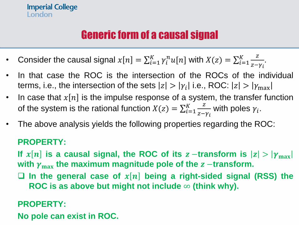
• Consider the causal signal 𝑥 𝑛 = σ𝑖=1𝐾 𝛾𝑖

𝑛𝑢[𝑛] with 𝑋(𝑧) = σ𝑖=1𝐾 𝑧

𝑧−𝛾𝑖.

• In that case the ROC is the intersection of the ROCs of the individual

terms, i.e., the intersection of the sets 𝑧 > 𝛾𝑖 i.e., ROC: 𝑧 > 𝛾max

• In case that 𝑥 𝑛 is the impulse response of a system, the transfer function

of the system is the rational function 𝑋(𝑧) = σ𝑖=1𝐾 𝑧

𝑧−𝛾𝑖with poles 𝛾𝑖.

• The above analysis yields the following properties regarding the ROC:

PROPERTY:

If 𝒙 𝒏 is a causal signal, the ROC of its 𝒛 −transform is 𝒛 > 𝜸𝐦𝐚𝐱

with 𝜸𝐦𝐚𝐱 the maximum magnitude pole of the 𝒛 −transform.

❑ In the general case of 𝒙 𝒏 being a right-sided signal (RSS) the

ROC is as above but might not include ∞ (think why).

PROPERTY:

No pole can exist in ROC.

Generic form of a causal signal

• The signal 𝑥 𝑛 = σ𝑖=1𝐾 𝛾𝑖

𝑛𝑢[𝑛] is bounded only if 𝛾𝑖 < 1 ∀𝑖 or 𝛾max < 1.

• In that case the ROC includes a circle with radius equal to 1. This is known

as the unit circle.

• The above observation yields the following property:

PROPERTY:

If the ROC of 𝑿(𝒛) includes the unit circle in 𝒛 −plane, then the signal

in time is bounded and its Discrete Time Fourier Transform exists.

• In case that 𝛾𝑛𝑢 𝑛 is part of a causal system’s impulse response, we see

that the condition 𝛾 < 1 must hold. This is because, since lim𝑛→∞

𝛾 𝑛 = ∞,

for 𝛾 > 1, the system will be unstable in that case.

• Therefore, in causal systems, stability requires that the ROC of the

system’s transfer function includes the unit circle.

Generic form of a causal signal cont.

• Find the 𝑧 −transform of the anti-causal signal −𝛾𝑛𝑢[−𝑛 − 1], where 𝛾 is a

constant.

• By definition:

𝑋[𝑧] =

𝑛=−∞

∞

−𝛾𝑛𝑢 −𝑛 − 1 𝑧−𝑛 =

𝑛=−∞

−1

−𝛾𝑛𝑧−𝑛 = −

𝑛=1

∞

𝛾−𝑛𝑧𝑛 = −

𝑛=1

∞𝑧

𝛾

𝑛

= −𝑧

𝛾

𝑛=0

∞𝑧

𝛾

𝑛

= −𝑧

𝛾1 +

𝑧

𝛾+

𝑧

𝛾

2

+𝑧

𝛾

3

+⋯

• Therefore,

𝑋[𝑧] = −𝑧

𝛾

1

1−𝑧

𝛾

, 𝑧

𝛾< 1

=𝑧

𝑧−𝛾, 𝑧 < 𝛾

• We notice that the 𝑧 −transform exists for certain values of 𝑧, which consist

the complement of the ROC of the function 𝛾𝑛𝑢[𝑛] with respect to the

𝑧 −plane.

Example: Find the 𝒛 −transform of 𝒙 𝒏 = −𝜸𝒏𝒖[−𝒏 − 𝟏]

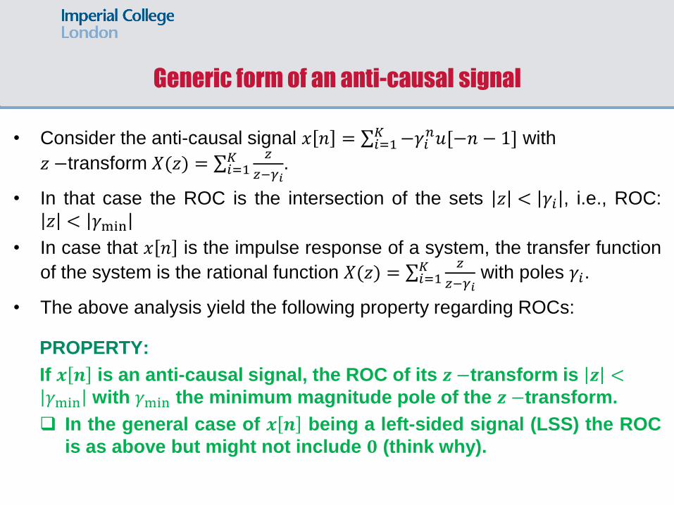
• Consider the anti-causal signal 𝑥 𝑛 = σ𝑖=1𝐾 −𝛾𝑖

𝑛𝑢[−𝑛 − 1] with

𝑧 −transform 𝑋(𝑧) = σ𝑖=1𝐾 𝑧

𝑧−𝛾𝑖.

• In that case the ROC is the intersection of the sets 𝑧 < 𝛾𝑖 , i.e., ROC:

𝑧 < 𝛾min

• In case that 𝑥 𝑛 is the impulse response of a system, the transfer function

of the system is the rational function 𝑋(𝑧) = σ𝑖=1𝐾 𝑧

𝑧−𝛾𝑖with poles 𝛾𝑖.

• The above analysis yield the following property regarding ROCs:

PROPERTY:

If 𝒙 𝒏 is an anti-causal signal, the ROC of its 𝒛 −transform is 𝒛 <𝛾min with 𝛾min the minimum magnitude pole of the 𝒛 −transform.

❑ In the general case of 𝒙 𝒏 being a left-sided signal (LSS) the ROC

is as above but might not include 𝟎 (think why).

Generic form of an anti-causal signal

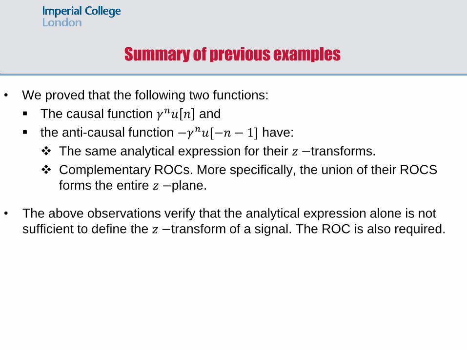
• We proved that the following two functions:

▪ The causal function 𝛾𝑛𝑢 𝑛 and

▪ the anti-causal function −𝛾𝑛𝑢[−𝑛 − 1] have:

❖ The same analytical expression for their 𝑧 −transforms.

❖ Complementary ROCs. More specifically, the union of their ROCS

forms the entire 𝑧 −plane.

• The above observations verify that the analytical expression alone is not

sufficient to define the 𝑧 −transform of a signal. The ROC is also required.

Summary of previous examples

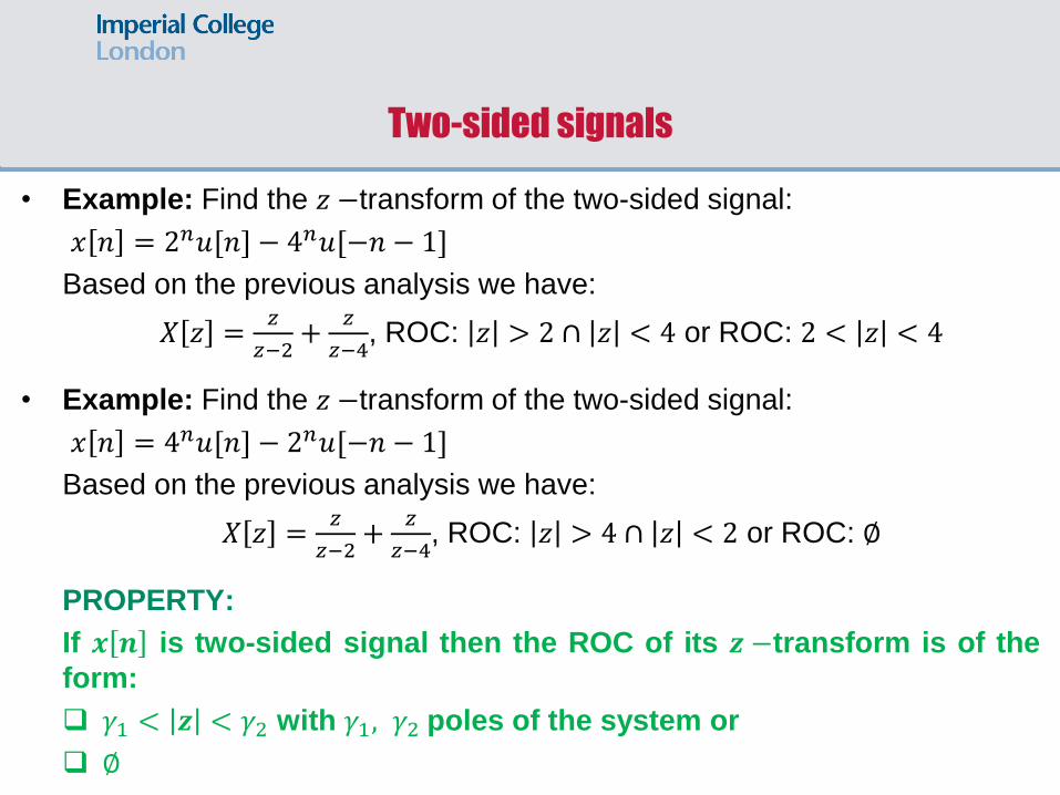
• Example: Find the 𝑧 −transform of the two-sided signal:

𝑥 𝑛 = 2𝑛𝑢[𝑛] − 4𝑛𝑢[−𝑛 − 1]

Based on the previous analysis we have:

𝑋 𝑧 =𝑧

𝑧−2+

𝑧

𝑧−4, ROC: 𝑧 > 2 ∩ 𝑧 < 4 or ROC: 2 < 𝑧 < 4

• Example: Find the 𝑧 −transform of the two-sided signal:

𝑥 𝑛 = 4𝑛𝑢[𝑛] − 2𝑛𝑢[−𝑛 − 1]

Based on the previous analysis we have:

𝑋 𝑧 =𝑧

𝑧−2+

𝑧

𝑧−4, ROC: 𝑧 > 4 ∩ 𝑧 < 2 or ROC: ∅

PROPERTY:

If 𝒙 𝒏 is two-sided signal then the ROC of its 𝒛 −transform is of the

form:

❑ 𝛾1 < 𝒛 < 𝛾2 with 𝛾1, 𝛾2 poles of the system or

❑ ∅

Two-sided signals

• By definition 𝛿 0 = 1 and 𝛿 𝑛 = 0 for 𝑛 ≠ 0.

𝑋[𝑧] =

𝑛=−∞

∞

𝛿 𝑛 𝑧−𝑛 = 𝛿 0 𝑧−0 = 1

• By definition 𝑢 𝑛 = 1 for 𝑛 ≥ 0.

𝑋[𝑧] = σ𝑛=−∞∞ 𝑢 𝑛 𝑧−𝑛 = σ𝑛=0

∞ 𝑧−𝑛 =1

1−1

𝑧

, 1

𝑧< 1

=𝑧

𝑧−1, 𝑧 > 1

Example: Find the 𝒛 −transform of 𝜹[𝒏] and 𝒖[𝒏]

• We write cos𝛽𝑛 =1

2𝑒𝑗𝛽𝑛 + 𝑒−𝑗𝛽𝑛 .

• From previous analysis we showed that:

𝛾𝑛𝑢[𝑛] ⇔𝑧

𝑧−𝛾, 𝑧 > 𝛾

• Hence,

𝑒±𝑗𝛽𝑛𝑢[𝑛] ⇔𝑧

𝑧−𝑒±𝑗𝛽, 𝑧 > 𝑒±𝑗𝛽 = 1

• Therefore,

𝑋 𝑧 =1

2

𝑧

𝑧−𝑒𝑗𝛽+

𝑧

𝑧−𝑒−𝑗𝛽=

𝑧(𝑧−cos𝛽)

𝑧2−2𝑧cos𝛽+1, 𝑧 > 1

Example: Find the 𝒛 −transform of 𝐜𝐨𝐬𝜷𝒏𝒖[𝒏]

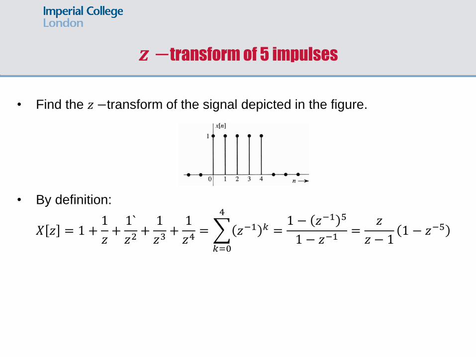
• Find the 𝑧 −transform of the signal depicted in the figure.

• By definition:

𝑋 𝑧 = 1 +1

𝑧+1`

𝑧2+1

𝑧3+1

𝑧4=

𝑘=0

4

𝑧−1 𝑘 =1 − 𝑧−1 5

1 − 𝑧−1=

𝑧

𝑧 − 11 − 𝑧−5

𝒛 −transform of 5 impulses

Inverse 𝒛 −transform

• As with other transforms, inverse 𝑧 −transform is used to derive 𝑥[𝑛]from 𝑋[𝑧], and is formally defined as:

𝑥 𝑛 =1

2𝜋𝑗ර𝑋[𝑧]𝑧𝑛−1𝑑𝑧

• Here the symbol ׯ indicates an integration in counter-clockwise

direction around a circle within the ROC and 𝑧 = 𝑅𝑒𝑗𝜃.

• Such contour integral is difficult to evaluate (but could be done using

Cauchy’s residue theorem), therefore we often use other techniques to

obtain the inverse 𝑧 −transform.

• One such technique is to use a 𝑧 −transform pairs Table shown in the

last two slides with partial fraction expansion.

Inverse 𝒛 −transform: Proof

Proof:

1

2𝜋𝑗ර𝑋[𝑧]𝑧𝑛−1𝑑𝑧 =

1

2𝜋𝑗ර

𝑚=−∞

∞

𝑥[𝑚]𝑧−𝑚 𝑧𝑛−1𝑑𝑧

= σ𝑚=−∞∞ 𝑥[𝑚]

1

2𝜋𝑗ׯ 𝑧𝑛−𝑚−1𝑑𝑧 = σ𝑚=−∞

∞ 𝑥[𝑚] 𝛿 𝑛 −𝑚 = 𝑥[𝑛]

❑ For the above we used the Cauchy’s theorem:

1

2𝜋𝑗ׯ 𝑧𝑘−1𝑑𝑧 = 𝛿 𝑘 for 𝑧 = 𝑅𝑒𝑗𝜃 anti-clockwise.

𝑑𝑧

𝑑𝜃= 𝑗𝑅𝑒𝑗𝜃 ⇒

1

2𝜋𝑗ׯ 𝑧𝑘−1𝑑𝑧 =

1

2𝜋𝑗𝜃=02𝜋

𝑅𝑘−1𝑒𝑗(𝑘−1)𝜃 𝑗𝑅𝑒𝑗𝜃𝑑𝜃 =

𝑅𝑘

2𝜋𝜃=02𝜋

𝑒𝑗𝑘𝜃 𝑑𝜃 = 𝑅𝑘 𝛿 𝑘

[ 𝑅𝑘

2𝜋𝜃=02𝜋

𝑒𝑗𝑘𝜃 𝑑𝜃 = ቐ0 𝑘 ≠ 0

𝑅𝑘

2𝜋2𝜋 = 𝑅𝑘 𝑘 = 0

]

Find the inverse 𝒛 −transform in the case of real unique poles

• Find the inverse 𝑧 −transform of 𝑋 𝑧 =8𝑧−19

(𝑧−2)(𝑍−3)

Solution

𝑋[𝑧]

𝑧=

8𝑧 − 19

𝑧(𝑧 − 2)(𝑍 − 3)=(−

196)

𝑧+

3/2

𝑧 − 2+

5/3

𝑧 − 3

𝑋 𝑧 = −19

6+

3

2

𝑧

𝑧−2+

5

3

𝑧

𝑧−3

By using the simple transforms that we derived previously we get:

𝑥 𝑛 = −19

6𝛿[𝑛] +

3

22𝑛 +

5

33𝑛 𝑢[𝑛]

Find the inverse 𝒛 −transform in the case of real repeated poles

• Find the inverse 𝑧 −transform of 𝑋 𝑧 =𝑧(2𝑧2−11𝑧+12)

(𝑧−1)(𝑧−2)3

Solution

𝑋[𝑧]

𝑧=

(2𝑧2−11𝑧+12)

(𝑧−1)(𝑧−2)3=

𝑘

𝑧−1+

𝑎0

(𝑧−2)3+

𝑎1

(𝑧−2)2+

𝑎2

(𝑧−2)

▪ We use the so called covering method to find 𝑘 and 𝑎0

𝑘 = อ(2𝑧2 − 11𝑧 + 12)

(𝑧 − 1)(𝑧 − 2)3𝑧=1

= −3

𝑎0 = อ(2𝑧2 − 11𝑧 + 12)

(𝑧 − 1)(𝑧 − 2)3𝑧=2

= −2

The shaded areas above indicate that they are excluded from the entire

function when the specific value of 𝑧 is applied.

Find the inverse 𝒛 −transform in the case of real repeated poles cont.

• Find the inverse 𝑧 −transform of 𝑋 𝑧 =𝑧(2𝑧2−11𝑧+12)

(𝑧−1)(𝑧−2)3

Solution

𝑋[𝑧]

𝑧=

(2𝑧2−11𝑧+12)

(𝑧−1)(𝑧−2)3=

−3

𝑧−1+

−2

(𝑧−2)3+

𝑎1

(𝑧−2)2+

𝑎2

(𝑧−2)

▪ To find 𝑎2 we multiply both sides of the above equation with 𝑧 and let

𝑧 → ∞.

0 = −3 − 0 + 0 + 𝑎2 ⇒ 𝑎2 = 3

▪ To find 𝑎1 let 𝑧 → 0.

12

8= 3 +

1

4+

𝑎1

4−

3

2⇒ 𝑎1 = −1

𝑋[𝑧]

𝑧=

(2𝑧2−11𝑧+12)

(𝑧−1)(𝑧−2)3=

−3

𝑧−1−

2

𝑧−2 3 −1

(𝑧−2)2+

3

(𝑧−2)⇒

𝑋 𝑧 =−3𝑧

𝑧−1−

2𝑧

𝑧−2 3 −𝑧

(𝑧−2)2+

3𝑧

(𝑧−2)

Find the inverse 𝒛 −transform in the case of real repeated poles cont.

𝑋 𝑧 =−3𝑧

𝑧−1−

2𝑧

𝑧−2 3 −𝑧

(𝑧−2)2+

3𝑧

(𝑧−2)

• We use the following properties:

▪ 𝛾𝑛𝑢[𝑛] ⇔𝑧

𝑧−𝛾

▪𝑛(𝑛−1)(𝑛−2)…(𝑛−𝑚+1)

𝛾𝑚𝑚!𝛾𝑛𝑢 𝑛 ⇔

𝑧

(𝑧−𝛾)𝑚+1

[−2𝑧

𝑧−2 3 = (−2)𝑧

𝑧−2 2+1 ⇔ (−2)𝑛(𝑛−1)

222!𝛾𝑛𝑢 𝑛 = −2

𝑛(𝑛−1)

8∙ 2𝑛𝑢[𝑛]

• Therefore,

𝑥 𝑛 = [−3 ∙ 1𝑛 − 2𝑛(𝑛−1)

8∙ 2𝑛 −

𝑛

2∙ 2𝑛 + 3 ∙ 2𝑛]𝑢[𝑛]

= − 3 +1

4𝑛2 + 𝑛 − 12 2𝑛 𝑢[𝑛]

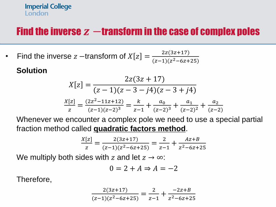
Find the inverse 𝒛 −transform in the case of complex poles

• Find the inverse 𝑧 −transform of 𝑋 𝑧 =2𝑧(3𝑧+17)

(𝑧−1)(𝑧2−6𝑧+25)

Solution

𝑋 𝑧 =2𝑧(3𝑧 + 17)

(𝑧 − 1)(𝑧 − 3 − 𝑗4)(𝑧 − 3 + 𝑗4)

𝑋[𝑧]

𝑧=

(2𝑧2−11𝑧+12)

(𝑧−1)(𝑧−2)3=

𝑘

𝑧−1+

𝑎0

(𝑧−2)3+

𝑎1

(𝑧−2)2+

𝑎2

(𝑧−2)

Whenever we encounter a complex pole we need to use a special partial

fraction method called quadratic factors method.

𝑋[𝑧]

𝑧=

2(3𝑧+17)

(𝑧−1)(𝑧2−6𝑧+25)=

2

𝑧−1+

𝐴𝑧+𝐵

𝑧2−6𝑧+25

We multiply both sides with 𝑧 and let 𝑧 → ∞:

0 = 2 + 𝐴 ⇒ 𝐴 = −2

Therefore,

2(3𝑧+17)

(𝑧−1)(𝑧2−6𝑧+25)=

2

𝑧−1+

−2𝑧+𝐵

𝑧2−6𝑧+25

Find the inverse 𝒛 −transform in the case of complex poles cont.

2(3𝑧+17)

(𝑧−1)(𝑧2−6𝑧+25)=

2

𝑧−1+

−2𝑧+𝐵

𝑧2−6𝑧+25

To find 𝐵 we let 𝑧 = 0:

−34

25= −2 +

𝐵

25⇒ 𝐵 = 16

𝑋[𝑧]

𝑧=

2

𝑧−1+

−2𝑧+16

𝑧2−6𝑧+25⇒ 𝑋 𝑧 =

2𝑧

𝑧−1+

𝑧(−2𝑧+16)

𝑧2−6𝑧+25

• We use the following property:

𝑟 𝛾 𝑛 cos 𝛽𝑛 + 𝜃 𝑢[𝑛] ⇔𝑧(𝐴𝑧+𝐵)

𝑧2+2𝑎𝑧+ 𝛾 2 with 𝐴 = −2, 𝐵 = 16, 𝑎 = −3, 𝛾 = 5.

𝑟 =𝐴2 𝛾 2+𝐵2−2𝐴𝑎𝐵

𝛾 2−𝑎2=

4∙25+256−2∙(−2)∙(−3)∙16

25−9= 3.2, 𝛽 = cos−1

−𝑎

𝛾= 0.927𝑟𝑎𝑑,

𝜃 = tan−1𝐴𝑎−𝐵

𝐴 𝛾 2−𝑎2= −2.246𝑟𝑎𝑑.

Therefore, 𝑥 𝑛 = [2 + 3.2 cos 0.927𝑛 − 2.246 ]𝑢[𝑛]

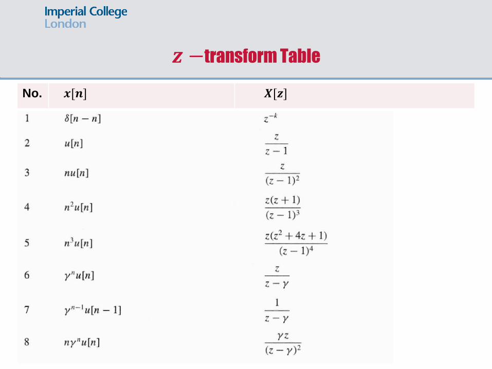
𝒛 −transform Table

No. 𝒙[𝒏] 𝑿[𝒛]

𝒛 −transform Table

No. 𝒙[𝒏] 𝑿[𝒛]