dsp integrated circuits, chapter 3 1 - linköping …dsp integrated circuits, chapter 3 8 since...
TRANSCRIPT
DSP Integrated Circuits, Chapter 3 1
3.1The Fourier transform is given by
(a) x(n)=an for n>0 and = 0 otherwise
X(ejωT) =
It is sum of a serial, the convegence is given by Abel theorem:
(i) is convergent
.
(ii ) is not convergent.
(ii i) is uncertain.
(b) x(n) = -an for n<0 and = 0 otherwise.
By using Abel theorem, we have
(i) is convergent. and
.
(ii ) is not convergent.
X ejωT( ) x nT( )e jnωT–
n ∞–=
∞
∑=
x nT( )e jnωT–
n ∞–=
∞
∑ anTe jnωT–
n 0=
∞
∑ aTe jωT–( )n
n 0=
∞
∑= =
aTe jωT– 1 i.e. aT 1 aTa jωT–( )n
n 0=
∞
∑,<,<
X ejωT( ) 11 aTe jωT––---------------------------=
aTe jωT– 1 or aT 1 aTa jωT–( )n
n 0=
∞
∑,>,>
aTe jωT– 1 the convergence of aTa jωT–( )n
n 0=
∞
∑,=
X ejωT( ) x nT( )e jnωT– anT– e jnωT– aTe jωT–( )n
a T– ejωT( )n
n 1=
∞
∑=
n ∞–=
1–
∑=
n ∞–=
1–
∑=
n ∞–=
∞
∑=
a T– ejωT 1 or aT 1 a T– ejωT( )n
n 1=
∞
∑–,>,<
X ejωT( ) a T– ejωT
1 a T– ejωT–---------------------------=
a T– ejωT 1 i.e. aT 1 a T– ejωT( )n
n 1=
∞
∑–,<,>
DSP Integrated Circuits, Chapter 3 2
(iii) is uncertain.
3.2
Apply the definition of z-transform to the sequences using Z{u(n)} =
(a) x1(nT)The period is 6, and the z-transform is
(b) x2(nT):The period is 7, and the z-transform is
(c) x3(nT)The period is 7, and the z-transform is
a T– ejωT 1 the convergence of a T– ejωT( )n
n 1=
∞
∑–,=
zz 1–-----------
Z x1 nT( ){ } x1 nT( )z n–
n ∞–=
∞
∑
0z0 az 1––– 0z 2– az 3– 0z 4– az 5––+ + +( )z 6n–
az 1–– az 3– az 5––+( )z 6n–
n 0=
∞
∑=
n 0=
∞
∑
az 1–– az 3– az 5––+( ) z 6n–
a z5 z3– z+( )–z6 1–
-----------------------------------=
n 0=
∞
∑
=
=
=
Z x2 nT( ){ } x2 nT( )z n–
n ∞–=
∞
∑=
0az0 az 1–– az 2–– a– z 3– az 4– az 5– az 6––+ + +( )z 7n–
az0 az 1– az 2–– az 3–– az 4– az 5– az 6––+ + +( ) z 7n–
a 1 z 1– z 2–– z 3–– z 4– z 5– z 6––+ + +( ) z7
z7 1–-------------
a z7 z6 z5– z4– z3 z2 z1–+ + +( )z7 1–
-------------------------------------------------------------------------------=
=
n 0=
∞
∑=
n 0=
∞
∑=
DSP Integrated Circuits, Chapter 3 3
(d) x4(nT)The period is 7, and the z-transform is
(e) x5(nT) :The period is 7, and the z-transform is
3.3 (a) x(n-n0)
Z x3 nT( ){ } x3 nT( )z n–
az0 0z 1–– az 2–– 0– z 3– az 4– 0z 5– az 6––+ + +( )z 7n–
az0 az 2–– az 4– az 6––+( ) z 7n–
n 0=
∞
∑=
n 0=
∞
∑=
n ∞–=
∞
∑
a z7 z5– z3 z1–+( )z7 1–
----------------------------------------------
=
=
Z x4 nT( ){ } x4 nT( )z n–
az0 0z 1– az 2–– a– z 3– 0z 4– az 5– 0z 6––+ + +( )z 7n–
az0 az 2–– az 3–– az 5––( ) z 7n–
n 0=
∞
∑=
n 0=
∞
∑=
n ∞–=
∞
∑
a z7 z5– z4– z2+( )z7 1–
----------------------------------------------
=
=
Z x5 nT( ){ } x5 nT( )z n–
az0 2az 1– az 2– a– z 3– 2az 4–– a– z 5– 0z 6–+ + +( )z 7n–
a 1 2z 1– z 2– z 3–– 2z 4–– z 5–– z 6–+ + +( ) z 7n–
n 0=
∞
∑=
n 0=
∞
∑=
n ∞–=
∞
∑
a z7 2z6 z5 z4– 2z3– z2– z1+ + +( )z7 1–
--------------------------------------------------------------------------------------
=
=
z n0– X z( )↔

DSP Integrated Circuits, Chapter 3 4
(b) anx(n)
(c) x(-n)
(d)
(Note: consider a complex number z = aeiθ, where a = |z| and θ is the argument, (zn)∗
= (aneinθ)∗ = (ane-inθ)∗ = (ae-iθ)n = (z∗)n,)
(e)
Z x n n0–( ){ } x n n0–( )z n–
n=-∞
∞
∑ x n n0–( )z n n0–( )– n0–
n=-∞
∞
∑
x n n0–( )z n n0–( )– z n0– z n0– x n n0–( )z n n0–( )– z n0– X z( )=
n=-∞
∞
∑=
n=-∞
∞
∑
= =
=
Xza---
↔
Z anx n( ){ } anx n( )z n–
n=-∞
∞
∑ x n( ) za---
n–
n=-∞
∞
∑ Xza---
= = =
X1z---
↔
Z x n–( ){ } x n–( )z n–
n=-∞
∞
∑ x m( )zm
m=-∞
∞
∑ x m( ) 1z---
m–
m=-∞
∞
∑ X1z---
= = = =
x∗ n( ) X∗ z∗( )↔
Z x∗ n( ){ } x∗ n( )z n–
n=-∞
∞
∑ x∗ n( ) z n–( )∗( )n=-∞
∞
∑ x∗ n( ) z n– ∗( )∗
x n( ) z∗( ) n–[ ]∗
n=-∞
∞
∑=
n=-∞
∞
∑
X∗ z∗( )
= = =
=
Re x n( ){ } 0,5 X z( ) X∗ z∗( )+[ ]↔Re x n( ){ } 0,5 X n( ) x∗ n( )+[ ]=
Z Re x n( ){ }{ } 0,5 x n( ) x∗ n( )+[ ]z n– 0,5 x n( )z n– x∗ n( )z n–+[ ]
0,5 x n( )z n– x∗ n( )z n–
n=-∞
∞
∑+
n=-∞
∞
∑
=
n=-∞
∞
∑=
n=-∞
∞
∑
0,5 X z( ) X∗ z∗( )+[ ]
=
=
DSP Integrated Circuits, Chapter 3 5
(f)
, in the same manner as (e), we have
.Alternatively, we can derive it from (e),since x(n) = , and Z{x(n)} = X(z), Z{Rex(n)}} = 0.5[X(z)+X*(z*)], with the linear property of z-transform,
Z{Im{x(n)}} = [Z{x(n)-Re{x(n)}}] = -0.5j[X(z)-X*(z*)].
3.4
(a) The autocorrelation function r(k) = .
Z{r(k)}=
(b) The convolution y(n) = .
Z{y(n)} =
3.5 We need to find a closed formulae for T(n), i.e., for the t ime required tosolve a large problem. We will do this by using the z - transform. However, we
Im x n( ){ } 0,5j X z( ) X∗ z∗( )–[ ]–↔Im x n( ){ } 0,5j x n( ) x∗ n( )–[ ]–=
Z Im x n( ){ }{ } 0,5j X z( ) X∗ z∗( )–[ ]–=
Re x n( ){ } j Im x n( ){ }⋅+
1j---
x n( )x∗ n k+( ) k 0≥( )n=0
∞
∑
r k( )z k–
k=-∞
∞
∑ x n( )x∗ n k+( )n=0
∞
∑
z k–
x n( )x∗ n k+( )z k–
k=0
∞
∑
n=0
∞
∑
=
k=0
∞
∑
x n( ) x∗ n k+( )z k–
k=0
∞
∑
x n( )zn X∗ z∗( )[ ]n=0
∞
∑=
n=0
∞
∑
X1z---
X∗ z∗( )
=
=
=
h k( )x n k–( )n=0
∞
∑
y n( )z n–
n=-∞
∞
∑ h k( )x n k–( )k=0
∞
∑
z n–
h k( ) x n k–( )z n–
n=0
∞
∑
h k( ) z k– X z( )[ ]k=0
∞
∑=
k=0
∞
∑=
n=0
∞
∑
X z( )H z( )
=
=

DSP Integrated Circuits, Chapter 3 6
first make the substitution.
in order to obtain a linear difference equation
where we for the sake of simplicity have selected MinSize = 1. Further, we haveassumed that the size of the subproblems is a power of cm, i.e., the subproblemshave sizes: n/c1, n/c2, n/c3, etc. Applying the z-transform yields
but the initial value, m = 0, yields x(0) = x(–1) + d = a ⇒⇒ x(–1) = a – d
and
x m( ) T cm( )bm
--------------=
x m( )a m 0=
x m 1–( ) dcm
bm---------+ m 0>
=
X z( ) z 1– X z( ) x 1–( )z+[ ] dcb---
mz m–
m 1=
∞
∑+=
X z( ) z 1– X z( ) a d– dcb---
mz m–
m 1=
∞
∑+ +=
X z( ) zz 1–----------- a d–
dz
zcb---–
-----------+=
a d–( )zz 1–
-------------------d
b c–----------- bz
z 1–-----------
cz
zcb---–
-----------–+=
x m( ) a d–bd
b c–-----------
cdb c–-----------
cb---
m–+ a d– d
1cb---
m 1+–
1cb---–
----------------------------+= = ⇒
DSP Integrated Circuits, Chapter 3 7
Thus
but .Finally, we get
.
We have three interesting cases.
Case: b < c
We get:
but we have
Hence, since, grows no faster than .
Case: b = c
For b=c we have
and
x m( ) a d– dcb---
i
i 0=
m
∑+= m 0≥,
T n( ) T cm( ) bm a d– dcb---
i
i 0=
m
∑+ a d–( )bm dcm bc---
i
i 0=
m
∑+= = =
m n( )clog=
T n( ) a d–( )b n( )clog dnbc---
i
i 0=
n( )clog
∑+=
T n( ) O a d–( )b n( )clog dnbc---
i
i 0=
n( )clog
∑+∈
T n( ) O a d–( )b n( )clog[ ] O dnbc---
i
i 0=
n( )clog
∑+∈ O b n( )clog[ ] O n( )+=
g n( )f n( )-----------
n ∞→lim
b n( )clog
n----------------
n ∞→lim
b n( )clog b( )lnn c( )ln
------------------------------n ∞→lim= = =
b n( )clog
n----------------
b( )lnc( )ln
-------------n ∞→lim= 0=
T n( ) O n( )∈ b n( )clog n
T n( ) a d–( )bm dn 1
i 0=
n( )clog
∑+ a d–( )n dn n( )clog 1+( )+= =
T n( ) O a d–( )n dn n( )clog 1+( )+[ ]∈ O n n( )clog[ ]=
DSP Integrated Circuits, Chapter 3 8
since
Case: b > cWe have
Finally we get:
3.9 A system is causal if and only ifx1(n) = x2(n) for if y1(n) = y2(n) for
Now, an LSI system is described by the convolution
We must have y1(n0) = y2(n0), =>
since for .
Thus, for since all terms in the convolution must be zero, i.e.,
for . On the other hand, if for , we have
=> is independent of for , i.e., independent of the future input samples.
3.6
nn n( )ln----------------
n ∞→lim 0=
T n( ) a d–( )bm dnbc---
i
i 0=
m
∑+ a d–( )bm dcm
1bc---
m 1+–
1bc---–
----------------------------+= =
T n( ) O a d–( )bm dcm
1bc---
m 1+–
1bc---–
----------------------------+∈ O bm[ ]=
T n( ) O b n( )clog[ ]∈ n b( )clog[ ]=
n n0≤ n n0≤
y n( ) x n( )h n k–( )k ∞–=
∞
∑=
y1 n0( ) y2 n0( )– x1 k( ) x2 k( )–[ ]h n0 k–( )k ∞–=
∞
∑ x1 k( ) x2 k( )–[ ]h n0 k–( )k n0=
∞
∑= =
x1 k( ) x2 k( )= k n0≤
h n0 k–( ) 0= k n0≤
h n( ) 0= n 0< h n( ) 0= n 0<
y n0( ) x n( )h n0 k–( )k ∞–=
∞
∑ x n( )h n0 k–( )k ∞–=
n0
∑= =
y n( ) x k( ) k n0>
H z( ) h n( )z n–
n ∞–=
∞
∑ 0.8( )nz n–
n ∞–=
∞
∑ 0.6( )nz n–
n ∞–=
∞
∑–= =
DSP Integrated Circuits, Chapter 3 9
The geometric series converges for:
|0.8 z–1| < 1 and |0.6 z–1| < 1, respectively. We get:
, |z| > 0.8
3.7 The step response is obtained by accumulating the impulse responsevalues:
Note that as .
Proof
for .
In this case we have and
3.8 The passband for the digital filter should be: fc = 25 kHz. Hence, the next image of the passband starts at: fsample – fc. From a filter table, or Delfi, we find that a third-order Butterworth filter, with 1 dB in the passband, has an attenuation of 40 dB at
6 fc = 150 kHz, i.e., (fsample – fc)/fc = 6 ⇒ fsample = 7 ⋅ 25 = 175 kHz
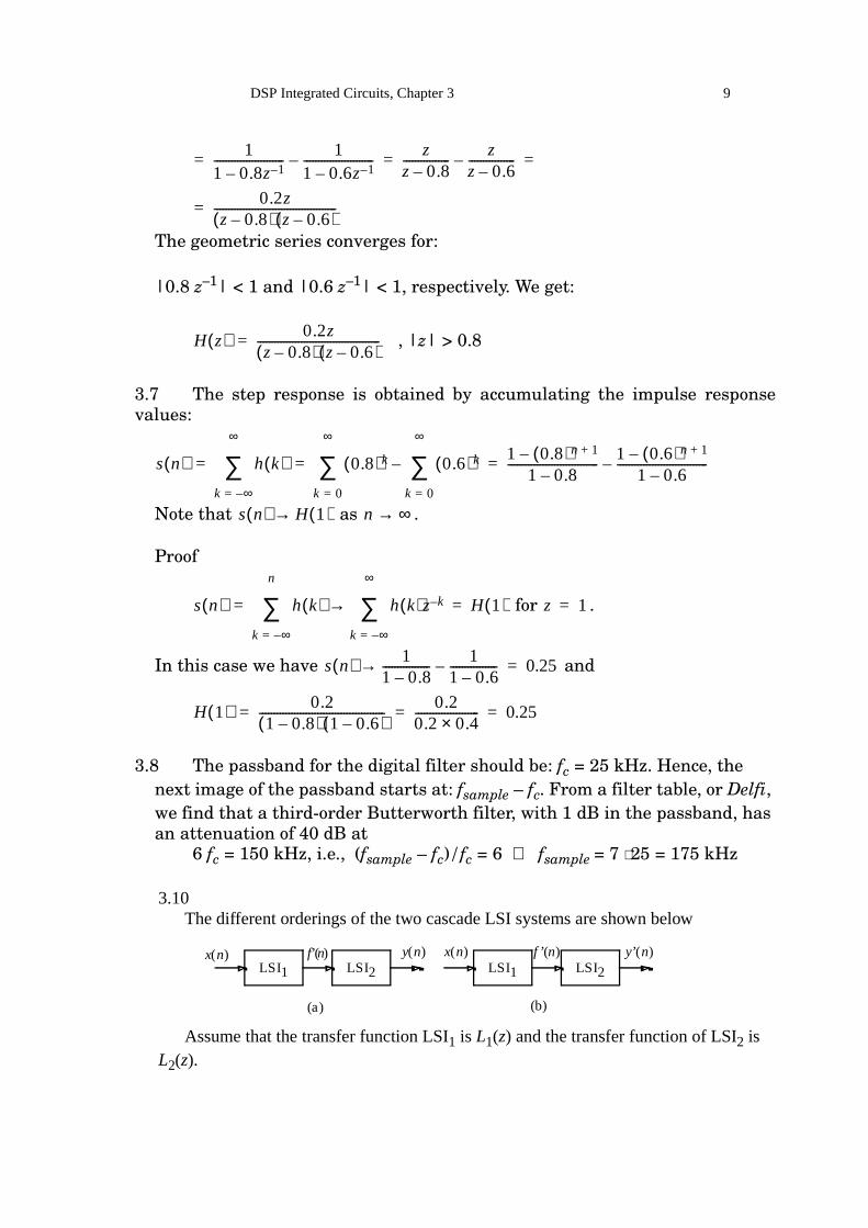
3.10The different orderings of the two cascade LSI systems are shown below
Assume that the transfer function LSI1 is L1(z) and the transfer function of LSI2 is L2(z).
11 0.8z 1––------------------------
11 0.6z 1––------------------------–=
zz 0.8–----------------
zz 0.6–----------------–= =
0.2zz 0.8–( ) z 0.6–( )
------------------------------------------=
H z( ) 0.2zz 0.8–( ) z 0.6–( )
------------------------------------------=
s n( ) h k( )k ∞–=
∞
∑ 0.8( )k
k 0=
∞
∑ 0.6( )k
k 0=
∞
∑–1 0.8( )n 1+–
1 0.8–-------------------------------
1 0.6( )n 1+–1 0.6–
-------------------------------–= = =
s n( ) H 1( )→ n ∞→
s n( ) h k( )k ∞–=
n
∑ h k( )z k–
k ∞–=
∞
∑→ H 1( )= = z 1=
s n( ) 11 0.8–----------------
11 0.6–----------------–→ 0.25=
H 1( ) 0.21 0.8–( ) 1 0.6–( )-------------------------------------------
0.20.2 0.4×---------------------- 0.25= = =
aa
LSI1 LSI2 LSI1 LSI2x(n) f’(n) y(n) x(n) f ’(n) y’(n)
(a) (b)
DSP Integrated Circuits, Chapter 3 10
For the system in (a), the z-transform of output y(n) can be calculated byY(z) = L2(z)F(z) = L2(z)L1(z)X(z);For the system in (b), the z-transform of output y’ (n) can be calculated byY’ (z) = L1(z)F’(z) = L1(z)L2(z)X(z).Since L1(z)L2(z) = L2(z)L1(z) according to the communitive law of multiplication,
we can state Y(z) = Y’ (z), i.e. the ordering of two cascade LSI systems may be inter-changed. 3.11
The difference equation is y(n) = by(n - 1) + ax(n). Apply z-transform to both sides of the equation we have
Y(z) = bz-1Y(z) + aX(z)which gives the transfer function
H(z) = = .
3.12a)
By identification we get
b) The region of convergence for the two geometric series are and
, respectively. The region of convergence for is where both series
convergences, i.e., .
Y z( )X z( )-----------
a1 bz 1––-------------------
H z( ) 1,2z 1,2+z2 1,6z– 0,63+-------------------------------------
11,4z 0,9–---------------
10,2z 0,7–---------------–
11,40,9---------- 0,9nz n–
n 1=
∞
∑ 10,20,7---------- 0,7nz n–
n 1=
∞
∑–
= =
=
h n( )0 n 1<
11,4 0,9n 1–× 10,2 0,7n 1–×– n 1≥
=
z 0,9>z 0,7> H z( )
z 0,9>
DSP Integrated Circuits, Chapter 3 11
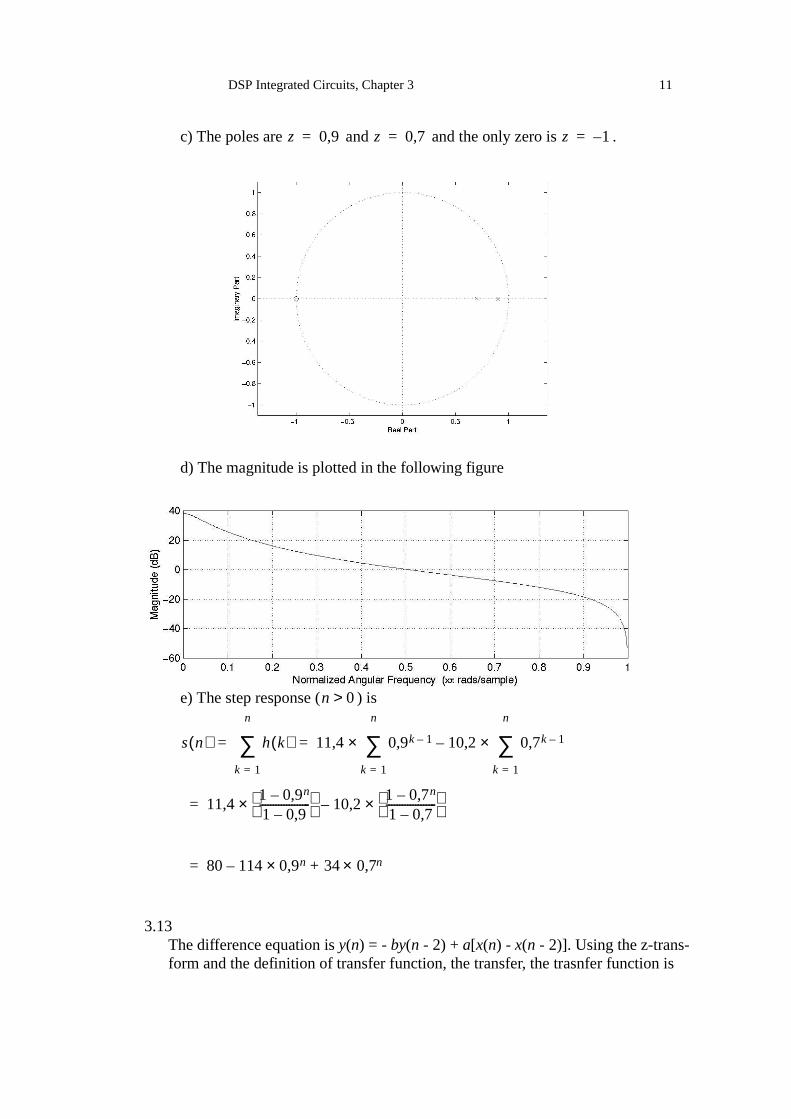
c) The poles are and and the only zero is .
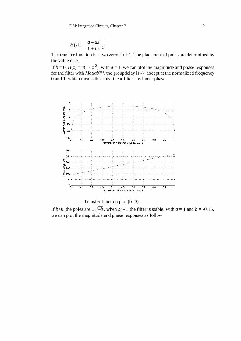
d) The magnitude is plotted in the following figure
e) The step response ( ) is
3.13The difference equation is y(n) = - by(n - 2) + a[x(n) - x(n - 2)]. Using the z-trans-form and the definition of transfer function, the transfer, the trasnfer function is
z 0,9= z 0,7= z 1–=
n 0>
s n( ) h k( )k 1=
n
∑ 11,4 0,9k 1–
k 1=
n
∑× 10,2 0,7k 1–
k 1=
n
∑×–
11,41 0,9n–1 0,9–-------------------
× 10,21 0,7n–1 0,7–-------------------
×–
80 114 0,9n×– 34 0,7n×+
= =
=
=
DSP Integrated Circuits, Chapter 3 12
The transfer function has two zeros in ± 1. The placement of poles are determined by the value of b.
If b = 0, H(z) = a(1 - z-2), with a = 1, we can plot the magnitude and phase responses for the filter with Matlab™. the groupdelay is -¼ except at the normalized frequency 0 and 1, which means that this linear filter has linear phase.
Transfer function plot (b=0)
If b<0, the poles are ± , when b>-1, the filter is stable, with a = 1 and b = -0.16, we can plot the magnitude and phase responses as follow
H z( ) a az 2––1 bz 2–+--------------------=
b–
DSP Integrated Circuits, Chapter 3 13
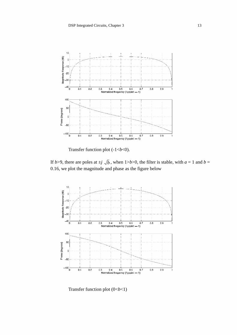
Transfer function plot (-1<b<0).
If b>9, there are poles at ±j , when 1>b>0, the fil ter is stable, with a = 1 and b = 0.16, we plot the magnitude and phase as the figure below
Transfer function plot (0<b<1)
b
DSP Integrated Circuits, Chapter 3 14
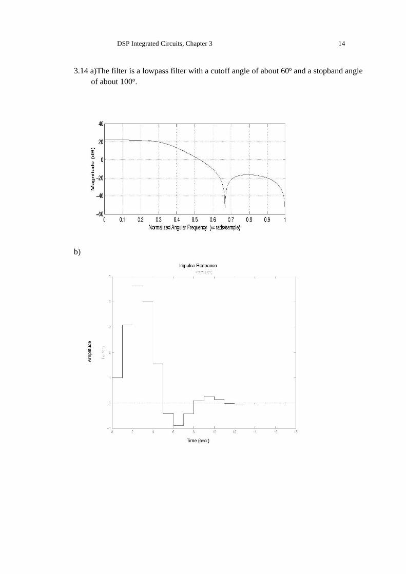
3.14 a)The filter is a lowpass filter with a cutoff angle of about 60o and a stopband angle of about 100o.
b)

DSP Integrated Circuits, Chapter 3 15
c) Changing the sign of the a- and b-coefficients in the second-order sections corre-sponds the changing the sign of real part of the poles and zeros. The pole-zero configura-tion is mirrored in the imaginary axis. Hence, the filter becomes a highpass filter. Thenew impulse response is
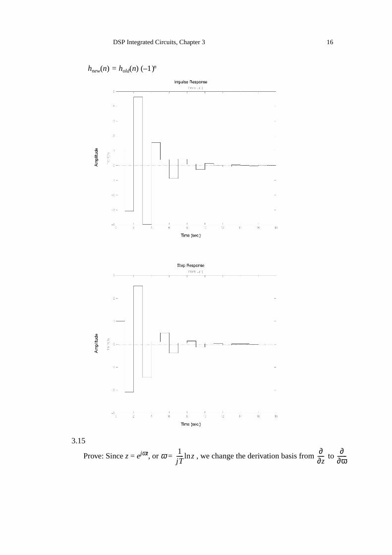
DSP Integrated Circuits, Chapter 3 16
hnew(n) = hold(n) (–1)n
3.15
Prove: Since z = ejωt, or ω = , we change the derivation basis from to 1jT----- zln
∂∂z-----
∂∂ω-------

DSP Integrated Circuits, Chapter 3 17
by .
The transfer function can be written as
The phase function is therefore Φ(z) = -j[lnH(z) - ln|H(z)|].
Compute the , we have
Change the derivation basis,
Since and are real functions, and
are therefore real functions, which gives that
Compare with the defination of group delay, we have
.
3.16In an electrocardiogram (E.C.G.) measurement, the form of a curve is important. The linearity of phase, which is predicted by group delay, is therefore a major inter-
∂∂z-----
dωdz-------
∂∂ω-------⋅
d1jT----- zln
dz----------------------
∂∂ω-------⋅ 1
jTz--------
∂∂ω-------⋅ je jωT–
T--------------
∂∂ω-------⋅= = = =
H z( ) H z( ) ejΦ z( )=
zddz----- H z( )ln
zddz----- H z( )ln z
ddz----- H z( ) ejΦ z( )[ ] z
ddz----- H z( ) j
ddz-----Φ z( )+ln
z
ddz----- H z( )
H z( )--------------------- j
ddz-----Φ z( )+
=
=ln=
zddz----- H z( )ln
zH z( )--------------
ddz----- H z( ) j H z( ) d
dz-----Φ z( )+
ejωT
H ejωT( )----------------------
je j– ωT
T--------------
∂∂ω------- H ejωT( ) e j– ωT
T------------ H ejωT( ) ∂
∂ω-------Φ ejωT( )+
1H ejωT( ) T-------------------------- H ejωT( ) ∂
∂ω-------Φ ejωT( ) j
∂∂ω------- H ejωT( )–
=
=
=
H ejωT( ) Φ ejωT( ) ∂∂ω------- H ejωT( ) ∂
∂ω-------Φ ejωT( )
Re zddz----- H z( )ln
Re1
H ejωT( ) T-------------------------- H ejωT( ) ∂
∂ω-------Φ ejωT( ) j
∂∂ω------- H ejωT( )–
1H ejωT( ) T-------------------------- H ejωT( ) ∂
∂ω-------Φ ejωT( )
1
T---
∂∂ω-------Φ ejωT( ).==
=
τg ωT( ) ∂∂ω-------Φ ωT( )– TRe z
ddz----- H z( )ln
for z– ejωT= = =

DSP Integrated Circuits, Chapter 3 18
est. If the group delay is over a limit, the form of curve is deformed which could lead to wrong judgement.
3.17 We have
3.18Using the notations of signals in the following figure, the difference equation can be written as:
e(n) = b(cy(n) + y(n - 1))w(n) = e(n) + x(n) = b(cy(n) + y(n - 1)) + x(n)y(n) = aw(n) + w(n-1)= ab(cy(n) + y(n -1)) + ax(n) + b(cy(n -1) + y(n - 2)) + x(n - 1)= b(acy(n) + (a + c)y(n - 1) + y(n - 1) + y(n - 2)) + ax(n) + x(n - 1)
Apply the z-transform to the difference equation, the transfer function is thereby
The zero is -a, and the poles are . The
sketch of polezero configuration is left to the reader to exploit the value combina-tions of a, b and c.
3.19 We have:
.
Thus, X(k) = X*(N–k)
H ejωT( ) 2 H ejωT( )H*ejωT( )= =
1 aejωT–ejωT a–
----------------------1 ae j– ωT–e j– ωT a–
-------------------------=1 ae j– ωT aejωT a2+––1 aejωT ae j– ωT a2+––-------------------------------------------------------- 1= =
aa
T
T
x(n) w(n) y(n)
b y(n-1)
bc y(n)
w(n-1)e(n)b
c
c
H z( ) a z 1–+1 abc–( ) b a c+( )z 1–– bz 2––
-------------------------------------------------------------------------=
b a c+( )– b ba2 2abc– bc2 4+ +( )±2 1– abc+( )
-----------------------------------------------------------------------------------------------
X k( ) x n( )Wnk
n 0=
N 1–
∑ x*
n( )Wnk
n 0=
N 1–
∑= = =
x n( )W nk–
n 0=
N 1–
∑*
x n( )W N k–( )n
n 0=
N 1–
∑*
X* N k–( )= = =
DSP Integrated Circuits, Chapter 3 19
3.22
Show that
where W = .
(i) If k = 0, .
(ii )If k ¦ 0, ,
With the results for (i) and (ii), we have shown that
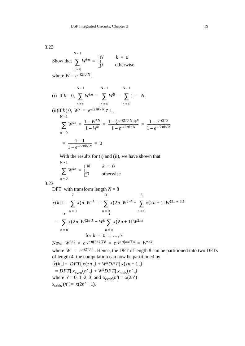
3.23DFT with transform length N = 8
for
Now,
where . Hence, the DFT of length 8 can be partitioned into two DFTs of length 4, the computation can now be partitioned by
where n’ = 0, 1, 2, 3, and xeven(n’) = x(2n’).xodds (n’) = x(2n’ + 1).
Wkn
n = 0
N - 1
∑N k 0=
0 otherwise
=
e i2π N⁄–
Wkn
n = 0
N - 1
∑ W0
n = 0
N - 1
∑ 1
n = 0
N - 1
∑ N= = =
Wk e i2πk N⁄– 1≠=
Wkn
n = 0
N - 1
∑ 1 WkN–1 Wk–-------------------
1 e i2π N⁄–( )kN–1 e i2πk N⁄––
-------------------------------------1 e i2πk––
1 e i2πk N⁄––-----------------------------
1 1–1 e i2πk N⁄––----------------------------- 0
= = =
= =
Wkn
n = 0
N - 1
∑N k 0=
0 otherwise
=
x k( ) x n( )Wnk
n = 0
7
∑ x 2n( )W2nk x 2n 1+( )W 2n 1+( )k
n = 0
3
∑+
n = 0
3
∑
x 2n( )W 2n( )k Wk x 2n 1+( )W2nk
n = 0
3
∑+
n = 0
3
∑
= =
=
k 0 1 … 7, , ,=
W2nk e jnπ 2nk( ) 8⁄– e jnπ nk( ) 4⁄– W′nk= = =
W′ e j2π 4⁄–=
x k( ) DFT x zn( ){ } WkDFT x zn 1+( ){ }DFT xeven n′( ){ } WkDFT xodds n′( ){ }+=
+=
DSP Integrated Circuits, Chapter 3 20
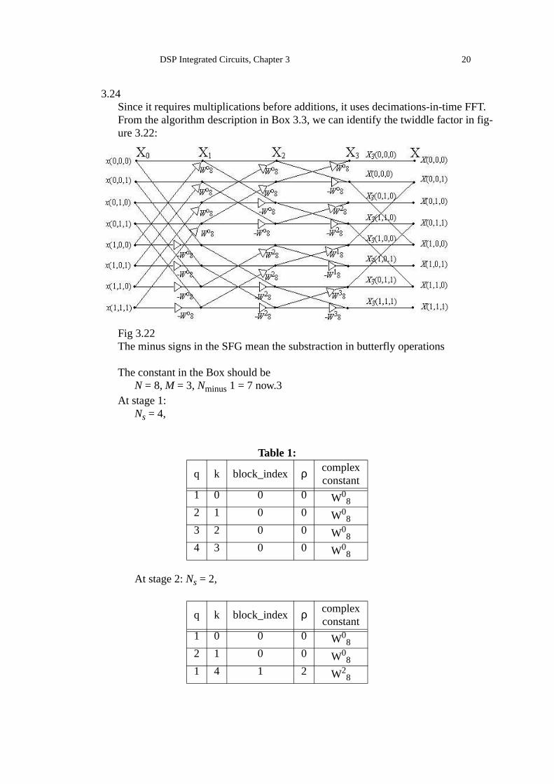
3.24Since it requires multiplications before additions, it uses decimations-in-time FFT. From the algorithm description in Box 3.3, we can identify the twiddle factor in fig-ure 3.22:
Fig 3.22The minus signs in the SFG mean the substraction in butterfly operations
The constant in the Box should beN = 8, M = 3, Nminus 1 = 7 now.3
At stage 1:Ns = 4,
At stage 2: Ns = 2,
Table 1:
q k block_index ρ complex constant
1 0 0 0 W08
2 1 0 0 W08
3 2 0 0 W08
4 3 0 0 W08
q k block_index ρ complex constant
1 0 0 0 W08
2 1 0 0 W08
1 4 1 2 W28

DSP Integrated Circuits, Chapter 3 21
At stage 3:Ns = 1,
3.26 Let Thus, we have obtained the IFFT except of the factor 1N . How-ever, this factor will, in practice, be included inside the butterflies in order to achieve a safe
scaling of the signals. and . According to the suggested algorithm we
start by computing the DFT of X(k). Hence, we compute the DFT where we have inter-changed the real and imaginary parts of discrete Fourier transform,
Now, we interchange the real and imaginary parts of the DFT
Thus, we have obtained the IFFT except of the factor 1/N . However, this factor will, in prac-tice, be included inside the butterflies in order to achieve a safe scaling of the signals.
2 5 1 2 W28
q k block_index ρ complex constant
1 0 0 0 W08
1 2 1 2 W28
1 4 2 1 W18
1 6 3 3 W38
q k block_index ρ complex constant
X n( ) A jB+=
Wnk WR jWI+=
X k( )
X n( )Wnk
n 0=
N 1–
∑ A jB+( ) WR jWI+( )n 0=
N 1–
∑= =
BWR jBWI jAWR AWI–+ +( )n 0=
N 1–
∑ ==
BWR AWI–( ) j BWI AWR+( )+[ ]n 0=
N 1–
∑ ==
BWR AWI–( ) j BWI AWR+( )+[ ]n 0=
N 1–
∑ =
A jB+( ) WR jWI–( )n 0=
N 1–
∑= =
A jB+( )W nk–
n 0=
N 1–
∑= X n( )W n– k
n 0=
N 1–
∑ x k( )= =

DSP Integrated Circuits, Chapter 3 22
An alternative method is as follows.
This alternative method to compute the IFFT by using two complex conjugate operations is more expensive than the method discussed above, since it involves two changes of the sign of the imaginary parts.
3.27 We form a new, complex-valued sequence from the two real-valuedsequences.
z(n) = x(n) + j y(n)
The DFT is .
Now, we compute the complex conjugate of the rotated Z(k) values
where.
Hence, we get .
Adding these two expressions we get:
Hence, Z(k) + Z*(N–k) = 2X(k) and X(k) = 0.5[Z(k) + Z*(N–k)]Similarly, subtracting the two expressions we get
Y(k) = –0.5 j[Z(k) – Z*(N–k)]Hence, the DFTs of two real-valued sequences can be computed simultaneously
x k( ) 1N---- X n( )W n– k
n 0=
N 1–
∑ 1N---- X n( )W n– k( )*
n 0=
N 1–
∑*
= = =
1N---- X* n( )Wnk
n 0=
N 1–
∑*
=1N---- DFT X* n( ){ }[ ]*=
Z k( ) z n( )Wnk
n 0=
N 1–
∑ z n( )e 2πn– k N⁄
n 0=
N 1–
∑= =
Z*
N k–( ) x n( ) jy n( )–[ ]e2πn N k–( ) N⁄
n 0=
N 1–
∑=
e2πn N k–( ) N⁄ e2πne 2– πnk N⁄ e 2– πnk N⁄= =
Z*
N k–( ) x n( ) jy n( )–[ ]e 2– πnk N⁄
n 0=
N 1–
∑=
Z k( ) Z*
N k–( )+ x n( ) jy n( )+[ ]e 2– πnk N⁄
n 0=
N 1–
∑ x n( ) jy n( )–[ ]e 2– πnk N⁄
n 0=
N 1–
∑+=
2x n( )e 2– πnk N⁄
n 0=
N 1–
∑=

DSP Integrated Circuits, Chapter 3 23
without any significant additional cost. The inverse DFT can be computed inthe same way.
3.29
where .
We can write the DCT in matrix form: .
The rows of C is referred to as the basis vectors. Desirable properties for the DCT are:
1. The same expression for the DCT transform and the inverse transform. Hence, only one algorithm need to be implemented.2. The application requires the DC component do not leak into other frequency components. This is due to the high DC content in images. We can view the DCT as a set of FIR filters. Hence, the filers must have a zero at z = 1, except for the first lowpass filter.3. The basis vectors should be symmetric or antisymmetric. This simplifies and reduces the hardware implementation.4. The transform should be orthogonal in order to efficiently decorrelate the images.
All of this properties cannot be satisfied simultaneously. We therefore relaxes the orthogonality requirement slightly. The matrix C is
X k( ) 2N 1–------------- ckx n( ) πnk
N 1–-------------
cos
n 0=
N 1–
∑= k 0 1 … N 1–, , ,=
ck
12--- for k 0 or k N 1–= =
1 for k 1 2 … N 2–, , ,=
=
X k( ) 2N 1–-------------Cx n( )=

DSP Integrated Circuits, Chapter 3 24
After simplification, we have:
3.30 PAL: N = (720 · 576 · 8 + 2 · 360 · 576 · 8) · = 166 Mbit/s
NTSC: N = (720 · 480 · 8 + 2 · 360 · 480 · 8) · = 166 Mbit/s
3.32 The sample frequency is 44.1 kHz. The resolution is given by the reciprocalof the FFT length. The length is
We get
3.33 a) DCT–I ↔ SDCTDCT–II ↔ EDCTDCT–IIIT (Transposed) ↔ DCT–IIDCT–IV is a shifted version of the SDCT
b) The relations derived i a) gives the kernel K for the inverse transforms.IDCT–I ↔ KDCT–I
T = KDCT–I
IDCT–II ↔ KDCT–IIT = KDCT–III
IDCT–III ↔ KDCT–IIIT = KDCT–II
IDCT–IV ↔ KDCT–IVT = KDCT–IV
502------
59.942
-------------
L 1024Tsample1024
44.1 103×-------------------------= =
∆f1L---
44.1 103×1024
------------------------- 43.07 Hz= = =