dsp_foehu - matlab 03 - the z-transform
TRANSCRIPT

MATLAB(03)
The z-Transform
Assist. Prof. Amr E. Mohamed
Z-Transform
Lecture Notes:
DSP_FOEHU - Lec 06 - The z-Transform
2
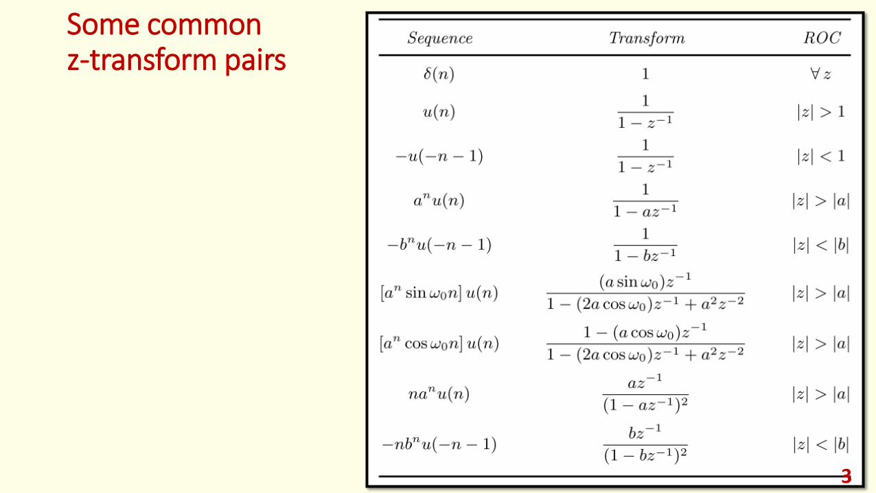
Some common z-transform pairs
3

Z-Transform Properties
4
Example #1
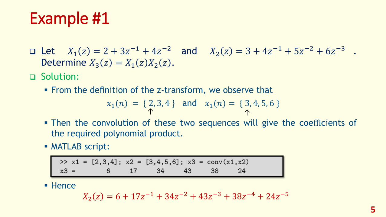
Let 𝑋1 𝑧 = 2 + 3𝑧−1 + 4𝑧−2 and 𝑋2 𝑧 = 3 + 4𝑧−1 + 5𝑧−2 + 6𝑧−3 .
Determine 𝑋3 𝑧 = 𝑋1 𝑧 𝑋2 𝑧 .
Solution:
From the definition of the z-transform, we observe that
𝑥1(𝑛) = { 2, 3, 4 } and 𝑥1(𝑛) = { 3, 4, 5, 6 }
Then the convolution of these two sequences will give the coefficients of
the required polynomial product.
MATLAB script:
Hence
𝑋2 𝑧 = 6 + 17𝑧−1 + 34𝑧−2 + 43𝑧−3 + 38𝑧−4 + 24𝑧−5
5
↑ ↑
Example #2
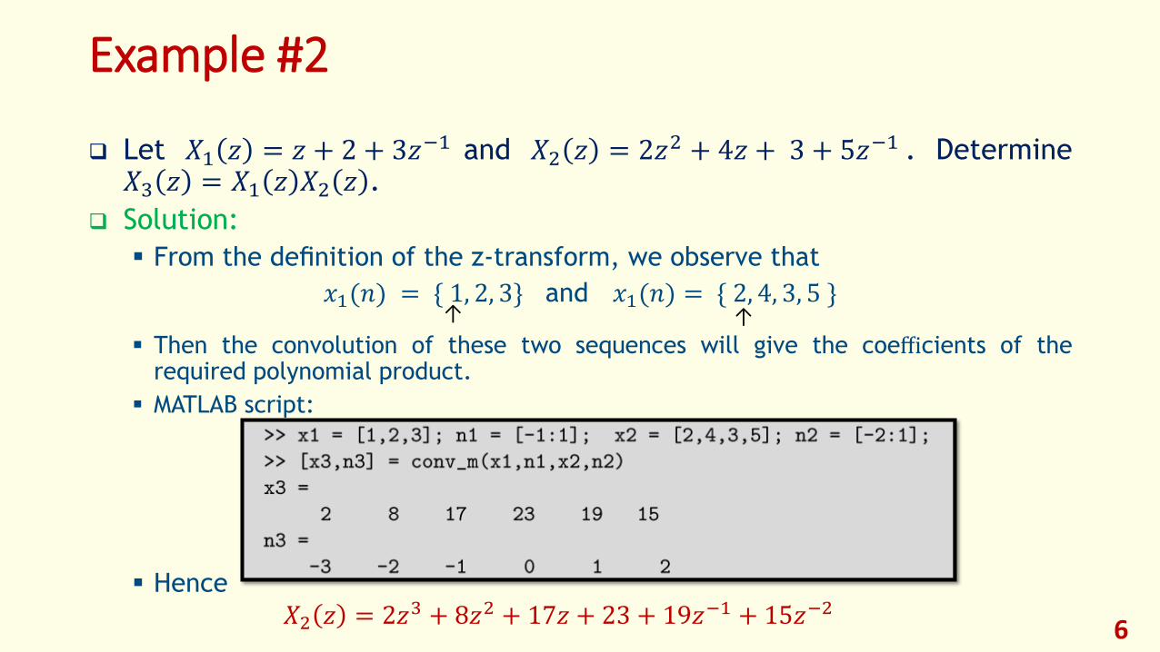
Let 𝑋1 𝑧 = 𝑧 + 2 + 3𝑧−1 and 𝑋2 𝑧 = 2𝑧2 + 4𝑧 + 3 + 5𝑧−1 . Determine𝑋3 𝑧 = 𝑋1 𝑧 𝑋2 𝑧 .
Solution:
From the definition of the z-transform, we observe that
𝑥1(𝑛) = { 1, 2, 3} and 𝑥1(𝑛) = { 2, 4, 3, 5 }
Then the convolution of these two sequences will give the coefficients of therequired polynomial product.
MATLAB script:
Hence
𝑋2 𝑧 = 2𝑧3 + 8𝑧2 + 17𝑧 + 23 + 19𝑧−1 + 15𝑧−26
↑ ↑
Note #1
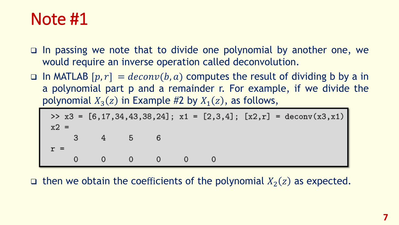
In passing we note that to divide one polynomial by another one, we
would require an inverse operation called deconvolution.
In MATLAB [𝑝, 𝑟] = 𝑑𝑒𝑐𝑜𝑛𝑣(𝑏, 𝑎) computes the result of dividing b by a in
a polynomial part p and a remainder r. For example, if we divide the
polynomial 𝑋3 𝑧 in Example #2 by 𝑋1 𝑧 , as follows,
then we obtain the coefficients of the polynomial 𝑋2 𝑧 as expected.
7

Note #2
Let 𝑥(𝑛) be a sequence with a rational transform
𝑋(𝑧) =𝐵(𝑧)
𝐴(𝑧)
where 𝐵(𝑧) and 𝐴(𝑧) are polynomials in 𝑧−1.
If we use the coefficients of 𝐵(𝑧) and 𝐴(𝑧) as the b and a arrays in the
filter routine and excite this filter by the impulse sequence 𝛿(𝑛), then
the output of the filter will be 𝑥(𝑛).
An equivalent approach is to use the 𝑖𝑚𝑝𝑧 function.
8

Note #2 (Cont.) Let 𝑥(𝑛) be
By z-transform
To check that this X(z) is indeed the correct expression, let us compute the first 8 samples of
the sequence x(n) corresponding to X(z), as discussed before.
9
Partial Fraction - Residue Calculation
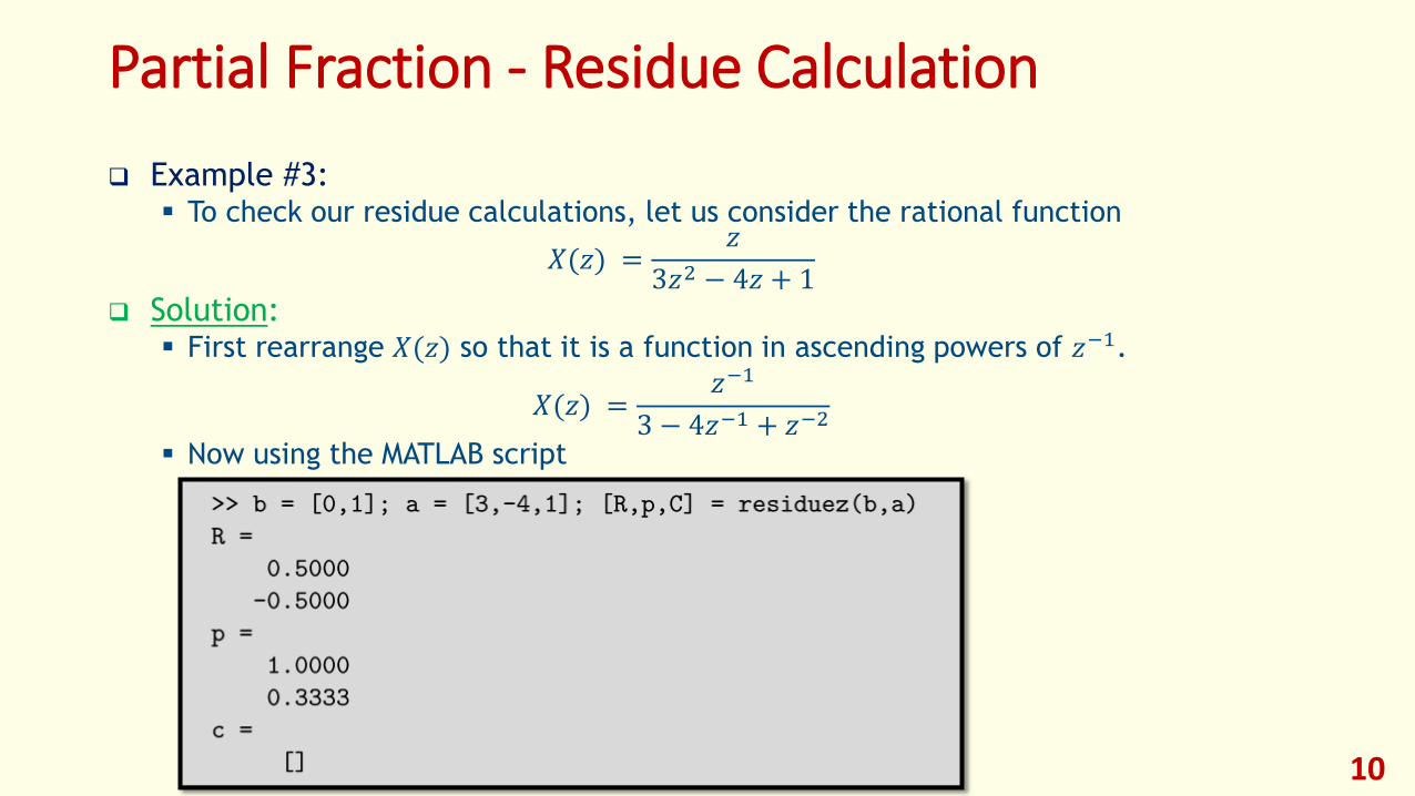
Example #3: To check our residue calculations, let us consider the rational function
𝑋(𝑧) =𝑧
3𝑧2 − 4𝑧 + 1 Solution:
First rearrange 𝑋(𝑧) so that it is a function in ascending powers of 𝑧−1.
𝑋(𝑧) =𝑧−1
3 − 4𝑧−1 + 𝑧−2
Now using the MATLAB script
10

Example #3 - Solution we obtain
𝑋 𝑧 =0.5
1 − 𝑧−1−
0.5
1 −13𝑧−1
as before. Similarly, to convert back to the rational function form,
so that
as before. 11

Example #4 Compute the inverse z-transform of
𝑋 𝑧 =1
1 − 0.9𝑧−1 2(1 + 0.9𝑧−1), 𝑧 > 0.9
Solution: We will evaluate the denominator polynomial as well as the residues using the MATLAB script:
12
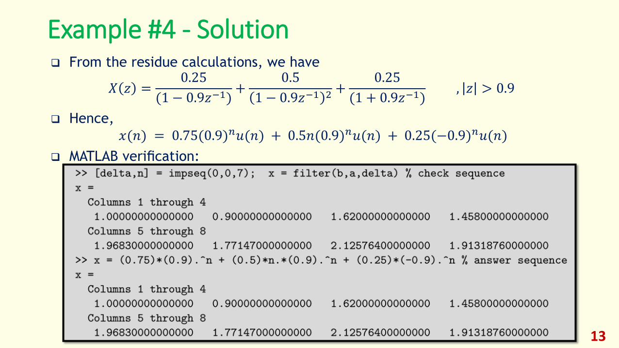
Example #4 - Solution From the residue calculations, we have
𝑋 𝑧 =0.25
(1 − 0.9𝑧−1)+
0.5
1 − 0.9𝑧−1 2 +0.25
(1 + 0.9𝑧−1), 𝑧 > 0.9
Hence,
𝑥(𝑛) = 0.75(0.9)𝑛𝑢(𝑛) + 0.5𝑛(0.9)𝑛𝑢(𝑛) + 0.25(−0.9)𝑛𝑢(𝑛)
MATLAB verification:
13
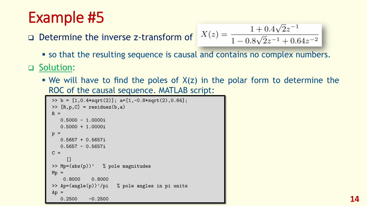
Example #5 Determine the inverse z-transform of
so that the resulting sequence is causal and contains no complex numbers.
Solution:
We will have to find the poles of X(z) in the polar form to determine the
ROC of the causal sequence. MATLAB script:
14
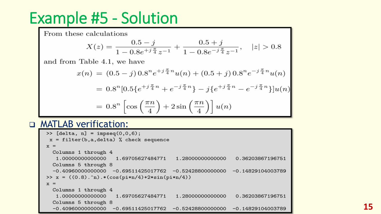
Example #5 - Solution
MATLAB verification:
15

SOLUTIONS OF THE DIFFERENCE EQUATIONS
16

Solutions Of The Difference Equations
In digital signal processing, difference equations generally evolve in the
positive 𝑛 direction. Therefore our time frame for these solutions will
be 𝑛 ≥ 0. For this purpose we define a version of the bilateral z-
transform called the one-sided z-transform.
17

Example #6
Solve
𝑦(𝑛) −3
2𝑦(𝑛 − 1) +
1
2𝑦(𝑛 − 2) = 𝑥(𝑛), 𝑛 ≥ 0
where
𝑥(𝑛) =1
4
𝑛
𝑢(𝑛)
subject to 𝑦( − 1) = 4 and 𝑦(− 2) = 10.
Solution:
Taking the one-sided z-transform of both sides of the difference equation,
we obtain
18
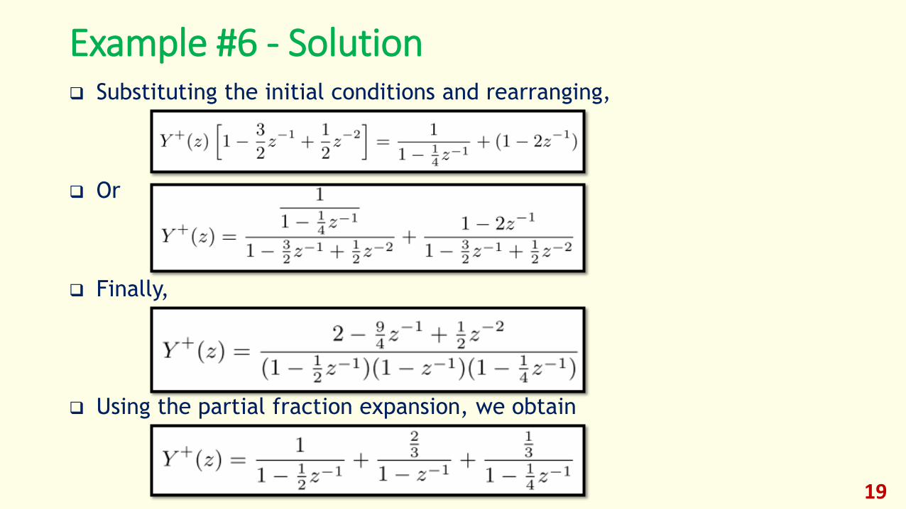
Example #6 - Solution Substituting the initial conditions and rearranging,
Or
Finally,
Using the partial fraction expansion, we obtain
19

Example #6 – Solution (Cont.)
After inverse transformation the solution is
20
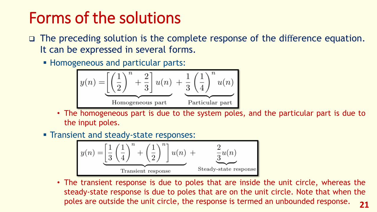
Forms of the solutions The preceding solution is the complete response of the difference equation.
It can be expressed in several forms.
Homogeneous and particular parts:
• The homogeneous part is due to the system poles, and the particular part is due to
the input poles.
Transient and steady-state responses:
• The transient response is due to poles that are inside the unit circle, whereas the
steady-state response is due to poles that are on the unit circle. Note that when the
poles are outside the unit circle, the response is termed an unbounded response. 21

Forms of the solutions (Cont.)
Zero-input (or initial condition) and zero-state responses:
In equation
𝑌 +(𝑧) has two parts. The first part can be interpreted as
while the second part as
where 𝑋IC (z) can be thought of as an equivalent initial-condition input that
generates the same output 𝑌ZI as generated by the initial conditions. In this
example 𝑥IC (n) is
22
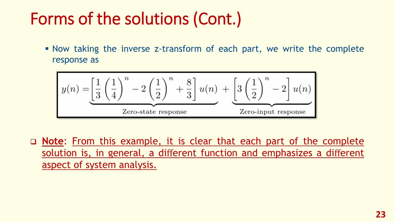
Forms of the solutions (Cont.)
Now taking the inverse z-transform of each part, we write the complete
response as
Note: From this example, it is clear that each part of the complete
solution is, in general, a different function and emphasizes a different
aspect of system analysis.
23

MATLAB Implementation
The 𝑓𝑖𝑙𝑡𝑒𝑟 function is used to solve the difference equation, given its
coefficients and an input.
where xic is an equivalent initial-condition input array.
To find the complete response in Example #6, we will use the MATLAB script
24

MATLAB Implementation (Cont.)
MATLAB provides a function called 𝑓𝑖𝑙𝑡𝑖𝑐, which is available only in the
Signal Processing toolbox. It is invoked by
If 𝑥(𝑛) = 0 , 𝑛 ≤ − 1 then 𝑋 need not be specified in the
𝑓𝑖𝑙𝑡𝑖𝑐 function. In Example #6, we could have used
to determine 𝑥IC (n) .
25
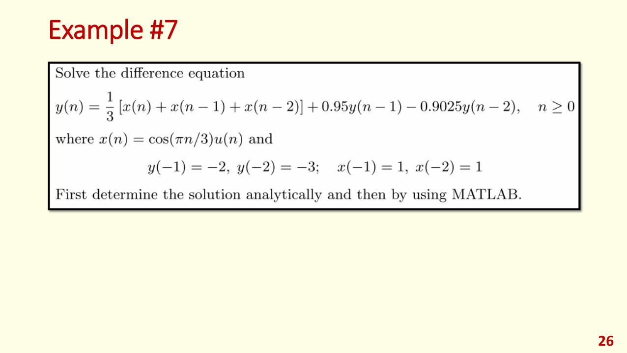
Example #7
26
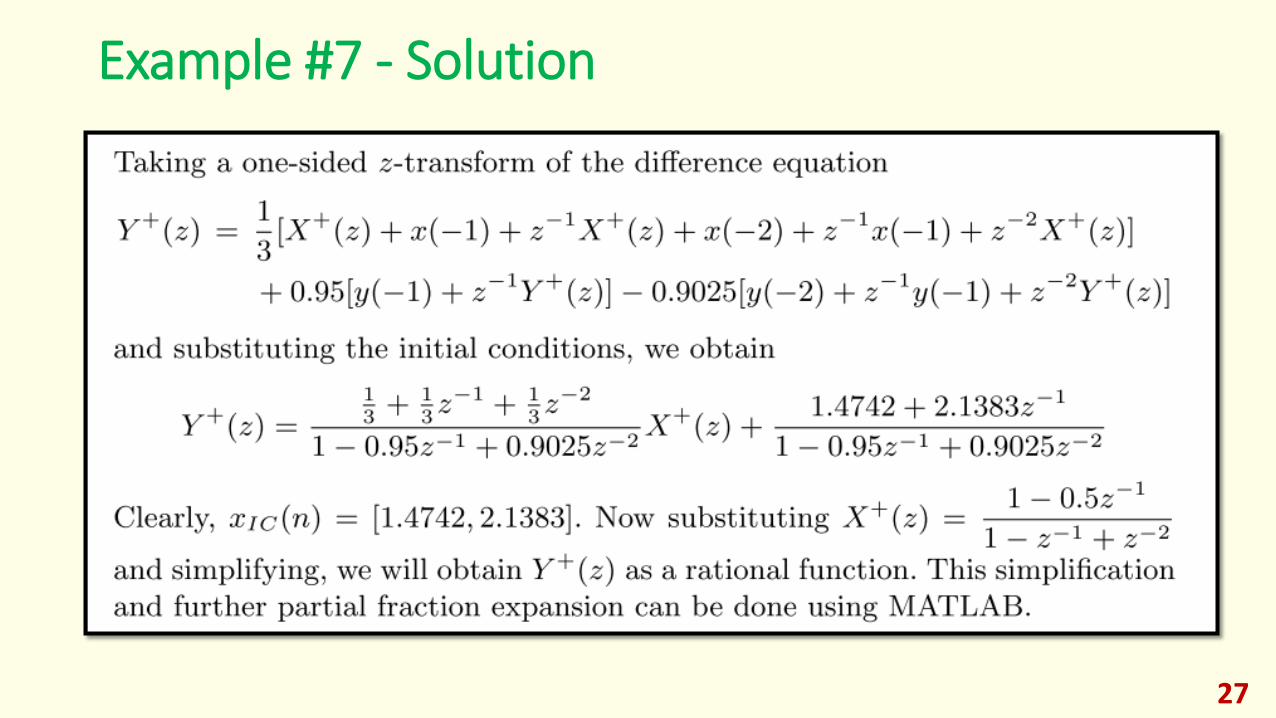
Example #7 - Solution
27

Example #7 – Solution (Cont.) MATLAB script:
28

29