Đstanbul technical university institute of science … (4).pdf · Đstanbul technical university...
TRANSCRIPT
Department : Geodesy & Photogrammetry Engineering
Programme : Geomatics Engineering
ĐSTANBUL TECHNICAL UNIVERSITY ���� INSTITUTE OF SCIENCE AND TECHNOLOGY
M.Sc. Thesis by Cihan UYSAL, Eng.
OCTOBER 2008
INTEGRATION OF REMOTE SENSING AND GEOGRAPHIC INFORMATION SYSTEMS IN
ARCHAEOLOGICAL APPLICATIONS

Date of submission : 17 September 2008
Date of defence examination: 21 October 2008
Supervisor (Chairman) : Prof. Dr. Derya MAKTAV (ITU)
Members of the Examining Committee : Prof. Dr. Zübeyde ALKI Ş (YTU)
Assoc. Prof. Dr. Gonca COŞKUN (ITU)
ĐSTANBUL TECHNICAL UNIVERSITY ���� INSTITUTE OF SCIENCE AND TECHNOLOGY
M.Sc. Thesis by Cihan UYSAL, Eng.
(501051607)
OCTOBER 2008
INTEGRATION OF REMOTE SENSING AND GEOGRAPHIC INFORMATION SYSTEMS IN
ARCHAEOLOGICAL APPLICATIONS

Tezin Enstitüye Verildiği Tarih : 17 Eylül 2008
Tezin Savunulduğu Tarih : 21 Ekim 2008
Tez Danışmanı : Prof. Dr. Derya MAKTAV ( ĐTÜ)
Diğer Jüri Üyeleri : Prof. Dr. Zübeyde ALKI Ş (YTÜ)
Doç. Dr. Gonca COŞKUN (ĐTÜ)
ĐSTANBUL TEKN ĐK ÜNĐVERSĐTESĐ ���� FEN BĐLĐMLER Đ ENSTĐTÜSÜ
YÜKSEK L ĐSANS TEZĐ
Cihan UYSAL
(501051607)
EKĐM 2008
ARKEOLOJ ĐK UYGULAMALARDA UZAKTAN ALGILAMA VE CO ĞRAFĐ BĐLGĐ SĐSTEMĐ
ENTEGRASYONU

FOREWORD I’m grateful to Prof. Dr. Derya Maktav and Prof. Dr. James Crow for his supports and instructions during preparation of my master thesis and also thankful to my family providing all kind of needs during my education. This work is supported by ITU Institute of Science and Technology. October 2008 Cihan UYSAL
Geodesy & Photogrammetry Engineering
ii
CONTENTS
FOREWORD …………………………………………………………………….... ii CONTENTS ……………………………………………………………………...... iii ABBREVIATIONS ………………………………………………………………... v TABLE LIST …………………………………………………………………….....vi FIGURE LIST ...........................................................................................................vii ABSTRACT……………………………………………………………………....... ix ÖZET……………………………………………………………………………....... x 1. INTRODUCTION ………………………………………………………………...1 2. FUNDAMENTALS OF ARCHAEOLOGY ……………………………………. 2
2.1. Definition of Archaeology……………………………………………………. 2 2.2. History of Archaeology………………………………………………………. 3 2.3. Excavation……………………………………………………………………..4 2.4. Surface Survey………………………………………………………………... 5
3. FUNDAMENTALS OF REMOTE SENSING AND GIS ………………...….....6 3.1. Fundamentals of Remote Sensing(RS)….…………………………....…......... 6 3.1.1 Basic Elements of Remote Sensing……………………………………....6 3.1.2 Electromagnetic Radiation………………………………………………. 7 3.1.3 Electromagnetic Spectrum………………………………………………. 9 3.1.4 Interactions with the Atmosphere……………………………………… 10 3.1.5 Radiation-Target Interactions………………………………………….. 12 3.1.6 Passive and Active Sensing……………………………………………..16 3.1.7 Spatial Resolution ……………………………………………………... 16 3.1.8 Spectral Resolution ……………………………………………………. 18 3.1.9 Radiometric Resolution ………………………………………………...19 3.1.10 Temporal Resolution…………………………………………………….21 3.2. Fundemantals of GIS ……………………………………………………….21 3.2.1 Definition of GIS………………………………………………………. 22 3.2.2 GIS Data Types………………………………………………………… 23 3.2.3 Data Sources…………………………………………………………… 24 4. IMPORTANCE OF REMOTE SENSING AND GIS IN ARCHAEOL OGY 25 4.1 GIS in Archaeology………………………………………………………….. 25 4.2 Remote Sensing in Archaeology……………………………………………... 28 5. APPLICATIONS ……………………………………………………………...... 32 5.1 Study Area…………………………………………………………………… 32 5.2 Data Used……………………………………………………………………. 33 5.2.1 ALOS………………………………………………………………….... 33 5.2.1.1 PRISM………………………………………………………………. 35 5.2.1.2 AVNIR-2……………………………………………………………. 36 5.2.1.3 PALSAR…………………………………………………………….. 37 5.3 Methods Used………………………………………………………………... 39
iii

5.3.1 Digital Terrain Model (DTM)…………………………………………… 39 5.3.2 DTM Generation From Topographical Maps…………………………… 39 5.3.3 DTM Generation From Stereo Images…………………………………... 40 5.3.4 DTM Generation From SRTM…………………………………………... 41 5.4 Methodology………………………………………………………………… 44 5.4.1 DTM Generation From Topographical Maps…………………………… 44 5.4.2 DTM Generation From SRTM…………………………………………... 46 5.4.3 DTM Generation From Stereo Images…………………………………... 47 5.4.4 Generation And Using GIS……………………………………………… 59 6. RESULTS……………………………………………………………………….. 61 REFERENCES …………………………………………………………………62 CURRICULUM VITAE ……………………………………………………….. 65
iv

ABBREVIATIONS
SRTM : Shuttle Radar Topography Mission
DEM : Digital Elevation Model
DTM : Digital Terrain Model
GIS : Global Positioning System
SAR : Synthetic Aperture Radar
HRS : High Resolution Stereoscopic
HRG : High Resolution Geometric
VHR : Very High Resolution
TIN : Triangular Irregular Network
GPS : Global Positioning System
FOV : Field of View
PALSAR : Phased Array type L-band Synthetic Aperture Radar
AVNIR : Advanced Visible and Near Infrared Radiometer
PRISM : Panchromatic Remote-sensing Instrument for Stereo Mapping
ALOS : Advanced Land Observing Satellite
TM : Thematic Mapper
NIR : Near Infrared
UV : Ultraviolet
v

LIST OF TABLES
Page No
Table 5.1: Characteristics of ALOS ……………………………………….......... 34 Table 5.2: Characteristics of PRISM …………………………………………… 36 Table 5.3: Observation modes of PRISM ………………………………………. 36 Table 5.4: Characteristics of AVNIR-2 ………………………………………… 37 Table 5.5: Characteristics of PALSAR …………………………………………. 38
vi
LIST OF FIGURES
Page No
Figure 3.1 Figure 3.2 Figure 3.3 Figure 3.4 Figure 3.5 Figure 3.6 Figure 3.7 Figure 3.8 Figure 3.9 Figure 3.10
: Elements of Remote Sensing........................................................... : Characteristics of electromagnetic radiation................................... : Wavelength and frequency.............................................................. : Electromagnetic spectrum............................................................... : Reflection of leaf............................................................................. : Reflection of vegetation.................................................................. : Reflection of water.......................................................................... : Spectral reflectance of some surface............................................. : Passive sensor.................................................................................. : Active sensor...................................................................................
6 8 8 9 12 13 14 15 16 16
Figure 3.11 Figure 3.12 Figure 3.13 Figure 3.14 Figure 3.15 Figure 3.16 Figure 4.1 Figure 4.2 Figure 4.3 Figure 4.4
: Instantaneous Field of View (IFOV).............................................. : Low Resolution............................................................................. : High Resolution.............................................................................. : Colour and Black & White Film..................................................... : Different Radiometric Resolution................................................... : Simplified Information System....................................................... : Three-dimensional image in ArcGlobe.......................................... : Predictive Modelling from Grisons, Swiss Alps............................ : Visual interpretation of main archaeological structures on IKONOS-2 imagery........................................................................
: Aerial photo of Gallo-Roman.........................................................
17 18 18 19 20 22 26 28 30 30
Figure 5.1 Figure 5.2 Figure 5.3 Figure 5.4 Figure 5.5 Figure 5.6 Figure 5.7 Figure 5.8 Figure 5.9 Figure 5.10
: Study Area..................................................................................... : Instruments of ALOS.................................................................... : PRISM........................................................................................... : Hillshade model…………………………………………………. : DTM……………………………………………………………... : DTM extracted from IKONOS-II stereo-pair................................ : SRTM instrument........................................................................... : Main antenna of SRTM.................................................................. : DEM generation from SRTM data............................................... : Contour line....................................................................................
32 34 35 40 40 41 42 43 44 45
Figure 5.11 Figure 5.12 Figure 5.13
: Triangle Irregular Network (TIN)……………………………….. : DTM Generation From Topographical Maps................................ : Overlapping of IKONOS Image on DTM Generated from Topographical Maps......................................................................
45 45 46
vii
Figure 5.31 : Generation and using GIS.............................................................. 60
Figure 5.14 Figure 5.15 Figure 5.16 Figure 5.17 Figure 5.18 Figure 5.19 Figure 5.20
: DTM Generation From SRTM........................................................ : Overlapping of IKONOS Image on DTM Generated from SRTM : ALOS Prism Image......................................................................... : Project Information......................................................................... : Projection Information.................................................................... : Data Input....................................................................................... : Format Changing............................................................................
46 47 48 49 49 51 51
Figure 5.21 Figure 5.22 Figure 5.23 Figure 5.24 Figure 5.25 Figure 5.26 Figure 5.27 Figure 5.28 Figure 5.29 Figure 5.30
: Reference Image............................................................................. : Working Image............................................................................... : Selection of GCP............................................................................ : All Grand Control Points................................................................ : RMS Value..................................................................................... : Generating Epipolar Image............................................................ : Automatic DEM Extraction............................................................ : DTM Generated From Prism Image............................................... : Study Area of DTM Generated From Prism Image....................... : Overlapping of IKONOS Image on DTM Generated from Prism Image...............................................................................................
52 52 53 55 55 56 57 58 58 59
viii
INTEGRATION OF REMOTE SENSING AND GEOGRAPHIC INFORM ATION SYSTEMS IN ARCHAEOLOGICAL APPLICATIONS
ABSTRACT
Recent improvements at satellite technologies and information systems has caused the frequently usage of remote sensing and integration of geographic information system. Especially, advances spatial resolution of satellite sensors, remote sensing technology has been used archaeological applications, too. In this study, Kurşunlugerme aqueduct, has been the important part water supply system at the time of Roman, Byzantine and Otoman Empires, and its environment has been chosen. The three dimensional model, which can get by overlaping satellite images onto regional digital terrain models, can provide the terrain topography to demonstrate. Vital analyses and comments will be made by adding GPS measurements at archaeological structures at study area. Moreover, in this study, digital terrain models can verify and compare by 1/25000 topographic maps, SRTM data, ALOS/PRISM stereo satellite images. For getting these results, a simple geographic information system will be used. By this system the results which will get by determining, analysing local water supply systems main lines, by usage of satellite data and terrain measurements, will be useful to gain national cultural heritage to the society.
ix

ARKEOLOJ ĐK UYGULAMALARDA UZAKTAN ALGILAMA VE CO ĞRAFĐ BĐLGĐ SĐSTEMĐ ENTEGRASYONU
ÖZET
Günümüzdeki uydu teknolojileri ve bilgi sistemlerindeki son gelişmeler, uzaktan algılama ve coğrafi bilgi sistemi entegrasyonunun birçok alanda daha yoğun bir biçimde kullanılmasına olanak sağlamıştır. Özellikle de uydu algılayıcılarının mekansal çözünürlüğünün her geçen gün artmasıyla birlikte, uzaktan algılama teknolojisi, arkeolojik çalışmalarda da kullanılmaya başlamıştır. Bu çalışmada, Roma, Bizans ve Osmanlı dönemlerinde Đstanbul’a su sağlayan su ikmal sistemlerinin önemli bir parçası olan Kurşunlugerme su kemeri ve çevresi çalışma alanı olarak seçilmiştir. Bölgenin dijital arazi modellerine çeşitli uydu görüntülerinin giydirilmesiyle elde edilecek üç boyutlu model ile arazi topoğrafyasının görselleştirilmesi sağlanacaktır. Bölgedeki arkeolojik yapıtlarla ilgili GPS ölçmeleri sonucu elde edilecek değerler bu model üzerine eklenerek gerekli analiz ve yorumlar yapılacaktır. Ayrıca bu çalışmada dijital arazi modelleri 1/25000 topoğrafik paftalardan, SRTM verilerinden, ALOS/PRISM stereo uydu görüntülerinden elde edilip doğrulukları karşılaştırılacaktır. Tüm bu sonuçlar basit bir coğrafi bilgi sistemi içerisinde sunulacaktır. Böyle bir sistem yardımıyla, uydu verileri ve yersel ölçmeler birlikte kullanılarak lokal su ikmal sistemlerine ait hatların belirlenmesi, analizi ve yorumlanmasıyla elde edilecek sonuçların, ülkemizin kültürel miraslarının topluma kazandırılması açısından yararlı olabileceği planlanmaktadır.
x
1
1. INTRODUCTION
Turkey has a remarkable strategical and geographical location that being influenced
by many empires during history. Therefore, Turkey has a rich cultural inheritance.
Istanbul in particular has a unique importance. There are many works of art that
remained from Rome , Byzantine and Ottoman Empire in Istanbul. Aqueducts which
brought water to towns and were main structures of water supplying systems can be
shown as an example of that kind of arts. A system that provided water for Istanbul
in ancient time, lies till 250-300 km west of city. Although there are many of
aqueducts, most of them are damaged or destroyed by some causes. Moreover, some
difficulties were appeared while revealing this aqueduct in detail because of
topography and searching large area. There are some uncertainty about route of
aqueduct in some areas. Classic terrestrial methods and archaeological methods are
used for this work. In addition, advanced satellite technology with developed spatial
resolution encourage users to manage archaeological work by using remote sensing
technology. Moreover, remote sensing with synoptic visual ability provides working
in large area and gives good results.
Kurşunlugerme province, aqueduct and its neighbours was chosen as working area.
First, the route of aqueduct is determined by GPS measurements in area. Satellite
images are also being used during determination and analyses. Correct analyses can
be made by using 3D models which formed as a result of overlaying satellite images
into digital terrain models. In this project the accuracy of digital terrain models will
be compared. For this purpose, digital elevation models will be formed by using
elevation data from 1/25000 maps, SRTM data and PRISM stereo satellite data and
accuracy will be evaluated. So geographic information system is established by using
3D models with digital elevation models, satellite images and GPS measurements.

2
2. FUNDAMENTALS OF ARCHAEOLOGY
2.1 Definition of Archaeology
Archaeology is partly the discovery of treasures of the past, partly the meticulous
work of the scientific analyst, partly the exercise of the creative imagination. It is
toiling in the sun on an excavation in the deserts of Iraq, it is working with living
Inuit in the snows of Alaska. It is diving down to Spanish wrecks off the coast of
Florida, and it is investigating the sewers of Roman York. But it is also the
painstaking task of interpretation so that we come to understand what these things
mean for the human story. And it is the conservation of the world’s cultural heritage
against looting and against careless destruction. Archaeology is the “past tense of
cultural anthropology.” Whereas cultural anthropologists will often base their
conclusions on the experience of actually living within contemporary communities,
archaeologists study past societies primarily through their material remains the
buildings, tools and other artifacts that constitute what is known as the material
culture left over from former societies (Renfrew and Bahn, 2000).
The objects that archaeologists discover, on the other hand, tell us nothing directly in
themselves. It is we today who have to make sense of these things. In this respect the
practice of archaeology is rather like that of the scientist. The scientist collects data
(evidence), conducts experiments, formulates a hypothesis (a proposition to account
for the data), tests the hypothesis against more data, and then in conclusion devises a
model (a description that seems best to summarize the pattern observed in the data).
The archaeologist has to develop a picture of past, just as the scientist has to develop
a coherent view of the natural world. It is not found ready made (Renfrew and Bahn,
2000).
As with most academic disciplines, there are a very large number of archaeological
sub-disciplines characterised by a specific method or type of material (e.g. lithic
analysis, music, archaeobotany), geographical or chronological focus (e.g. Near

3
Eastern archaeology, Medieval archaeology), other thematic concern (e.g. maritime
archaeology, landscape archaeology, battlefield archaeology), or a specific
archaeological culture or civilisation (e.g. Egyptology) [1].
In generally, archaeology includes various of classifications that changes according
to time periods and characteristic of civilization during that time periods such as
prehistorical and classical archaeology. Classical archaeology consists of period of
Hellenic and Rome civilizations that called archaic age. Prehistorical archaeology
aims to investigate cultural, economical and technological development of humanity
from the beginnig of life until founding of literary [2].
2.2 History of Archaeology
In the broadest sense, just as archaeology is an aspect of antropology, so too is it a
part of history, where we mean the whole history of humankind from its beginnings
over 3 million years ago. Indeed for more than 99 percent of that huge span of time
archaeology, the study of past material culture, is the only significant source of
information, if one sets aside physical anthropology, which focuses on our biological
rather than cultural progress. Conventional historical sources begin only with the
introduction of written records around 3000 BC in Western Asia, and much later in
most other parts of the world (not until AD 1788 in Australia, for example). A
commonly drawn distinction is between prehistory, the period before written records,
and history in the narrow sense, meaning the study of the past using written
evidence. In some countries, “prehistory” is now considered a patronizing and
derogatory term which implies that written texts are more valuable than oral
histories, and which classifies their cultures as inferior until the arrival of western
ways of recording information. To archaeology, however, which studies all cultures
and periods, whether with or without writing, the distinction between history and
prehistory is a convenient dividing linet hat simply recognizes the importances of
written word in the modern world, but in no way denigrates the useful information
contained in oral histories (Renfrew and Bahn, 2000).
The history of archaeology, then, is a history of new ideas, methods and discoverios.
Modern archaeology took root in the 19th century with the acceptance of three key
concepts: the great antiquity of humanity, Darwins’s principle of evolution, and the
Three Age System for ordering material culture. Many of the early civilizations,

4
especially in the old world, had been discovered by the 1880s, and some of their
ancient scripts deciphered. This was followed by a long phase of consolidation of
improvements in fieldwork and excavation and the establishment of regional
chronologies (Renfrew and Bahn, 2000).
After World War II the pace of change in the discipline quickened. New ecological
approaches sought to help us understand human adaptation to the environment. New
scientific techniques introduced among other things reliable means of dating the
prehistoric past. Spurred on by these developments, the new archaeology of the
1960s and 1970s turned to questions not just of what happened when, but why they
happened, in an attempt to explain processes of change. Meanwhile, Pioneer
fieldworkers studying whole regions opened up a truly world archaeology in time
and space in time back from the present to the earliest toolmakers, and in space
across all the world’s continents. More recently a diversity of theoretical approaches,
often grouped under the label postprocessual, highlighted the variety of possible
interpretations and the sensitivity of their politicial implications (Renfrew and Bahn,
2000).
2.3 Excavation
Excavation retains its central role in fieldwork because it yields the most reliable
evidence for the two main kinds of information archaeologists are interested in:
human activities at a particular period in the past; and changes in those activities
from period to period. Very broadly we can say that contemporary activities take
place horizontally in space, wheras changes in those activities occur vertically
through time. It is this distinction between horizontal slices of time and vertical
sequences through time that forms the basis of most excavation methodology.
Despite the growing importance of survey, the only way to check the reliability of
surface data, confirm the accuracy of the remote sensing techniques, and actually see
what remains of these sites is to excavate them. Furthermore, survey can tell us a
little about a large area, but only excavation can tell us a great deal about a relatively
small area (Renfrew and Bahn, 2000).
In the 18th century more adventurous researchers initiated excavation of some of the
most prominent sites. Pompeii in Italy was one of the first of these, with its striking
Roman finds, although proper excavation did not begin there until the 19th century.

5
And in 1765, at the Huaca de Tantalluc on the coast of Peru, a mound was excavated
and an offering was discovered in a hollow; the mound’s stratigraphy was well
described (Renfrew and Bahn, 2000).
2.4 Surface Survey
The simplest way to gain some idea of a site’s extent and layout is through a site
surface archaeology by studying the distribution of surviving features, and recording
and possibly collecting artifacts from the surface. Surface survey has a vital place in
archaeological work, and one that continues to grow in importance. In modern
projects, however, it is usually supplemented by reconnaissance from the air, one of
the most important advances made by archaeology this century. In fact, the
availability of air photographs can be an important factor in selecting and delineating
an area for surface survey. Until the present century, individual sites were the main
focus of archaeological attention, and the only remote sensing devices used were a
pair of eyes and a stick. The developments of aerial photography and reconnaissance
techniques have shown archaeologists that the entire landscape is of interest, while
geophysical and geochemical methods have revolutionized our ability to detect what
lies hidden beneath the soil (Renfrew and Bahn, 2000).
Today archaeologists study whole regions, often employing sampling techniques to
bring ground reconnaissance (surface survey) within the scope of individual research
teams. Having located sites within those regions, and mapped them using aerial
reconnaissance techniques and now GIS, archaeologists can then turn to a whole
battery of remote sensing site survey devices able to detect buried features without
excavation. The geophysical methods almost all involve either passing energy into
the ground and locating buried features from their effect on that energy or measuring
the intensity of the earth’s magnetic field. In either case, they depend on contrast
between the buried features and their surroundings. Many of the techniques are
costly in both equipment and time, but they are often cheaper and certainly less
destructive than random test pits or trial trenches. They allow archaeologiest to be
more selective in deciding which parts of a site, if any, should be fully excavated
(Renfrew and Bahn, 2000).

6
3. FUNDAMENTALS OF REMOTE SENSING (RS) AND GIS
3.1 Fundamentals of Remote Sensing (RS)
Remote sensing can be defined as the acquisition and recording of information about
an object without being in direct contact with that object (Gibson, 2000).
In much of remote sensing, the process involves an interaction between incident
radiation and the targets of interest. This is exemplified by the use of imaging
systems where the following seven elements are involved (Figure 3. 1). These seven
elements comprise the remote sensing process from beginning to end. Note, however
that remote sensing also involves the sensing of emitted energy and the use of non-
imaging sensors.
Figure 3. 1: Elements of Remote Sensing.
3.1.1 Basic Elements of RS
A. Energy source or ıllumination – the first requirement for remote sensing is to have
an energy source which illuminates or provides electromagnetic energy to the target
of interest.

7
B. Radiation and the atmosphere – as the energy travels from its source to the target,
it will come in contact with and interact with the atmosphere it passes through. This
interaction may take place a second time as the energy travels from the target to the
sensor.
C. Interaction with the target - once the energy makes its way to the target through
the atmosphere, it interacts with the target depending on the properties of both the
target and the radiation.
D. Recording of energy by the sensor - after the energy has been scattered by, or
emitted from the target, we require a sensor (remote - not in contact with the target)
to collect and record the electromagnetic radiation.
E. Transmission, reception, and processing - the energy recorded by the sensor has to
be transmitted, often in electronic form, to a receiving and processing station where
the data are processed into an image (hardcopy and/or digital).
F. Interpretation and analysis - the processed image is interpreted, visually and/or
digitally or electronically, to extract information about the target which was
illuminated.
G. Application - the final element of the remote sensing process is achieved when we
apply the information we have been able to extract from the imagery about the target
in order to better understand it, reveal some new information, or assist in solving a
particular problem [7].
3.1.2 Electromagnetic Radiation
The first requirement for remote sensing is to have an energy source to illuminate the
target (unless the sensed energy is being emitted by the target). This energy is in the
form of electromagnetic radiation. All electromagnetic radiation has fundamental
properties and behaves in predictable ways according to the basics of wave theory.
Electromagnetic radiation consists of an electrical field(E) which varies in magnitude
in a direction perpendicular to the direction in which the radiation is traveling, and a
magnetic field (M) oriented at right angles to the electrical field (Figure 3. 2). Both
these fields travel at the speed of light (c) [7].

8
Figure 3. 2: Characteristics of electromagnetic radiation.
Two characteristics of electromagnetic radiation are particularly important for
understanding remote sensing. These are the wavelength and frequency (Figure 3. 3).
Figure 3. 3: Wavelength and frequency.
Therefore, the two are inversely related to each other. The shorter the wavelength,
the higher the frequency. The longer the wavelength, the lower the frequency.
Understanding the characteristics of electromagnetic radiation in terms of their
wavelength and frequency is crucial to understanding the information to be extracted
from remote sensing data [7].

9
3.1.3 Electromagnetic Spectrum
The electromagnetic spectrum ranges from the shorter wavelengths (including
gamma and (x-rays) to the longer wavelengths (including microwaves and broadcast
radio waves). There are several regions of the electromagnetic spectrum which are
useful for remote sensing (Figure 3. 4).
Figure 3.4: Electromagnetic spectrum.
For most purposes, the ultraviolet or UV portion of the spectrum has the shortest
wavelengths which are practical for remotesensing. This radiation is just beyond the
violet portion of the visible wavelengths, hence its name. Some Earth surface
materials, primarily rocks and minerals, fluoresce or emit visible light when
illuminated by UV radiation.
The light which our eyes - our "remote sensors" - can detect is part of the visible
spectrum. It is important to recognize how small the visible portion is relative to the
rest of the spectrum. There is a lot of radiation around us which is "invisible" to our
eyes, but can be detected by other remote sensing instruments and used to our
advantage. The visible wavelengths cover a range from approximately 0.4 to 0.7 µm.
The longest visible wavelength is red and the shortest is violet. Blue, green, and red
are the primary colours or wavelengths of the visible spectrum. They are defined as
such because no single primary colour can be created from the other two, but all
other colours can be formed by combining blue, green, and red in various
proportions. Although we see sunlight as a uniform or homogeneous colour, it is
actually composed of various wavelengths of radiation in primarily the ultraviolet,

10
visible and infrared portions of the spectrum. The visible portion of this radiation can
be shown in its component colours when sunlight is passed through a prism, which
bends the light in differing amounts according to wavelength. The next portion of the
spectrum of interest is the infrared (IR) region which covers the wavelength range
from approximately 0.7 µm to 100 µm - more than 100 times as wide as the visible
portion! The infrared region can be divided into two categories based on their
radiation properties - the reflected IR, and the emitted or thermal IR. Radiation in the
reflected IR region is used for remote sensing purposes in ways very similar to
radiation in the visible portion. The reflected IR covers wavelengths from
approximately 0.7 µm to 3.0 µm. The thermal IR region is quite different than the
visible and reflected IR portions, as this energy is essentially the radiation that is
emitted from the Earth's surface in the form of heat. The thermal IR covers
wavelengths from approximately 3.0 µm to 100 µm. The portion of the spectrum of
more recent interest to remote sensing is the microwave region from about 1 mm to 1
m. This covers the longest wavelengths used for remote sensing. The shorter
wavelengths have properties similar to the thermal infrared region while the longer
wavelengths approach the wavelengths used for radio broadcasts.
3.1.4 Interactions with the Atmosphere
All radiation used for remote sensing must pass through the earth’s atmosphere. If
the sensor is carried by a low flying aircraft, effects of the atmosphere upon image
quality may be negligible. In contrast, energy that reaches sensors carried by earth
satellites must pass through the entire depth of the earth’s atmosphere. Under these
conditions, atmospheric effects may have substantial impact upon the quality of
images and data that the sensors generate. Therefore, the practice of remote sensing
requires knowledge of interactions of electromagnetic energy with the atmosphere
(Campbell, 2002).
Scattering occurs when particles or large gas molecules present in the atmosphere
interact with and cause the electromagnetic radiation to be redirected from its
original path. How much scattering takes place depends on several factors including
the wavelength of the radiation, the abundance of particles or gases, and the distance
the radiation travels through the atmosphere. There are three types of scattering
which take place. Rayleigh scattering occurs when particles are very small compared

11
to the wavelength of the radiation. These could be particles such as small specks of
dust or nitrogen and oxygen molecules. Rayleigh scattering causes shorter
wavelengths of energy to be scattered much more than longer wavelengths. Rayleigh
scattering is the dominant scattering mechanism in the upper atmosphere. The fact
that the sky appears "blue" during the day is because of this phenomenon. As
sunlight passes through the atmosphere, the shorter wavelengths (i.e. blue) of the
visible spectrum are scattered more than the other (longer) visible wavelengths. At
sunrise and sunset the light has to travel farther through the atmosphere than at
midday and the scattering of the shorter wavelengths is more complete; this leaves a
greater proportion of the longer wavelengths to penetrate the atmosphere.
Mie scattering occurs when the particles are just about the same size as the
wavelength of the radiation. Dust, pollen, smoke and water vapour are common
causes of Mie scattering which tends to affect longer wavelengths than those
affected by Rayleigh scattering. Mie scattering occurs mostly in the lower portions of
the atmosphere where larger particles are more abundant, and dominates when cloud
conditions are overcast.
The final scattering mechanism of importance is called nonselective scattering. This
occurs when the particles are much larger than the wavelength of the radiation.
Water droplets and large dust particles can cause this type of scattering. Nonselective
scattering gets its name from the fact that all wavelengths are scattered about
equally. This type of scattering causes fog and clouds to appear white to our eyes
because blue, green, and red light are all scattered in approximately equal quantities
(blue+green+red light = white light) [7].
Absorption is the other main mechanism at work when electromagnetic radiation
interacts with the atmosphere. In contrast to scattering, this phenomenon causes
molecules in the atmosphere to absorb energy at various wavelengths. Ozone, carbon
dioxide, and water vapour are the three main atmospheric constituents which absorb
radiation. Ozone serves to absorb the harmful (to most living things) ultraviolet
radiation from the sun. Without this protective layer in the atmosphere our skin
would burn when exposed to sunlight [7].

12
3.1.5 Radiation - Target Interactions
Radiation that is not absorbed or scattered in the atmosphere can reach and interact
with the Earth's surface. There are three forms of interaction that can take place when
energy strikes, or is incident (I) upon the surface. These are: absorption (A);
transmission (T); and reflection (R) (Figure 3. 5). The total incident energy will
interact with the surface in one or more of these three ways. The proportions of each
will depend on the wavelength of the energy and the material and condition of the
feature.
Figure 3. 5: Reflection of leaf.
Absorption (A) occurs when radiation (energy) is absorbed into the target while
transmission (T) occurs when radiation passes through a target. Reflection (R) occurs
when radiation "bounces" off the target and is redirected. In remote sensing, we are
most interested in measuring the radiation reflected from targets. We refer to two
types of reflection, which represent the two extreme ends of the way in which energy
is reflected from a target: specular reflection and diffuse reflection. When a surface is
smooth we get specular or mirror-like reflection where all (or almost all) of the
energy is directed away from the surface in a single direction. Diffuse reflection
occurs when the surface is rough and the energy is reflected almost uniformly in all
directions. Most earth surface features lie somewhere between perfectly specular or
perfectly diffuse reflectors. Whether a particular target reflects specularly or
diffusely, or somewhere in between, depends on the surface roughness of the feature
in comparison to the wavelength of the incoming radiation. If the wavelengths are
much smaller than the surface variations or the particle sizes that make up the
surface, diffuse reflection will dominate. For example, finegrained sand would

13
appear fairly smooth to long wavelength microwaves but would appear quite rough
to the visible wavelengths. There are some examples of targets at the Earth's surface
and how energy at the visible and infrared wavelengths interacts with them.
Leaves: A chemical compound in leaves called chlorophyll strongly absorbs
radiation in the red and blue wavelengths but reflects gren wavelengths. Leaves
appear "greenest" to us in the summer, when chlorophyll content is at its maximum.
In autumn, there is less chlorophyll in the leaves, so there is less absorption and
proportionately more reflection of the red wavelengths, making the leaves appear red
or yellow (yellow is a combination of red and green wavelengths). The internal
structure of healthy leaves act as excellent diffuse reflectors of near-infrared
wavelengths. If our eyes were sensitive to near-infrared, trees would appear
extremely bright to us at these wavelengths. In fact, measuring and monitoring the
near-IR reflectance is one way that scientists can determine how healthy (or
unhealthy) vegetation may be (Figure 3. 6).
Figure 3. 6: Reflection of vegetation.
Water: Longer wavelength visible and near infrared radiation is absorbed more by
water than shorter visible wavelengths. Thus water typically looks blue or blue-green
due to stronger reflectance at these shorter wavelengths, and darker if viewed at red
or near infrared wavelengths (Figure 3. 7). If there is suspended sediment present in
the upper layers of the water body, then this will allow better reflectivity and a
brighter appearance of the water. The apparent colour of the water will show a slight
shift to longer wavelengths. Suspended sediment (S) can be easily confused with
shallow (but clear) water, since these two phenomena appear very

14
similar. Chlorophyll in algae absorbs more of the blue wavelengths and reflects the
green, making the water appear more green in colour when algae is present. The
topography of the water surface (rough, smooth, floating materials, etc.) can also
lead to complications for water-related interpretation due to potential problems of
specular reflection and other influences on colour and brightness [7].
Figure 3. 7: Reflection of water.
When solar radiation hits a target surface, it may be transmitted, absorbed or
reflected. Different materials reflect and absorb differently at different wavelengths.
The reflectance spectrum of a material is a plot of the fraction of radiation reflected
as a function of the incident wavelength and serves as a unique signature for the
material. In principle, a material can be identified from its spectral reflectance
signature if the sensing system has sufficient spectral resolution to distinguish its
spectrum from those of other materials. This premise provides the basis for
multispectral remote sensing. The following graph shows the typical reflectance
spectra of five materials: clear water, turbid water, bare soil and two types of
vegetation (Figure 3. 8) (Campbell, 2002).
15
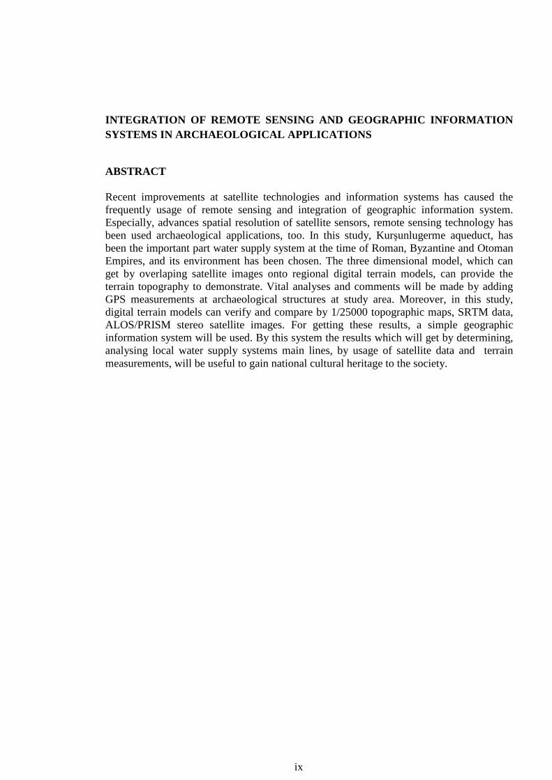
Figure 3. 8: Spectral reflectance of some surface.
Vegetation has a unique spectral signature which enables it to be distinguished
readily from other types of land cover in an optical/near-infrared image. The
reflectance is low in both the blue and red regions of the spectrum, due to absorption
by chlorophyll for photosynthesis. It has a peak at the green region which gives rise
to the green colour of vegetation. In the near infrared (NIR) region, the reflectance is
much higher than that in the visible band due to the cellular structure in the leaves.
Hence, vegetation can be identified by the high NIR but generally low visible
reflectances. This property has been used in early reconnaisance missions during war
times for "camouflage detection".
The shape of the reflectance spectrum can be used for identification of vegetation
type. For example, the reflectance spectra of vegetation 1 and 2 in the above figures
can be distinguished although they exhibit the generally characteristics of high NIR
but low visible reflectances. Vegetation 1 has higher reflectance in the visible region
but lower reflectance in the NIR region. For the same vegetation type, the reflectance
spectrum also depends on other factors such as the leaf moisture content and health
of the plants [8].

16
3.1.6 Passive and Active Sensing
There are two basic types of sensors: passive and active sensors. Passive sensors
record radiation reflected from the earth's surface (Figure 3. 9). The source of this
radiation must come from outside the sensor; in most cases, this is solar energy.
Because of this energy requirement, passive solar sensors can only capture data
during daylight hours. The Thematic Mapper (TM) sensor system on the Landsat
satellite is a passive sensor [9].
Active sensors are different from passive sensors. Unlike passive sensors, active
sensors require the energy source to come from within the sensor (Figure 3. 10). For
example, a laser-beam remote sensing system is an active sensor that sends out a
beam of light with a known wavelength and frequency. This beam of light hits the
earth and is reflected back to the sensor, which records the time it took for the beam
of light to return [9].
Figure 3.9: Passive sensor. Figure 3.10: Active sensor.
3.1.7 Spatial Resolution
The detail discernible in an image is dependent on the spatial resolution of the sensor
and refers to the size of the smallest possible feature that can be detected. Spatial
resolution of passive sensors depends primarily on their Instantaneous Field of View
(IFOV) (Figure 3. 11). The IFOV is the angular cone of visibility of the sensor (A)
and determines the area on the Earth's surface which is "seen" from a given altitude
at one particular moment in time (B). The size of the area viewed is determined by
multiplying the IFOV by the distance from the ground to the sensor (C). This area on
the ground is called the resolution cell and determines a sensor's maximum spatial

17
resolution. For a homogeneous feature to be detected, its size generally has to be
equal to or larger than the resolution cell. If the feature is smaller than this, it may not
be detectable as the average brightness of all features in that resolution cell will be
recorded. However, smaller features may sometimes be detectable if their reflectance
dominates within a articular resolution cell allowing sub-pixel or resolution cell
detection.
Figure 3.11: Instantaneous Field of View (IFOV).
Most remote sensing images are composed of a matrix of picture elements, or pixels,
which are the smallest units of an image. Image pixels are normally square and
represent a certain area on an image. It is important to distinguish between pixel size
and spatial resolution - they are not interchangeable. If a sensor has a spatial
resolution of 20 meters and an image from that sensor is displayed at full resolution,
each pixel represents an area of 20m x 20m on the ground. In this case the pixel size
and resolution are the same. However, it is possible to display an image with a pixel
size different than the resolution. Many posters of satellite images of the Earth have
their pixels averaged to represent larger areas, although the original spatial resolution
of the sensor that collected the imagery remains the same. Images where only large
features are visible are said to have coarse or low resolution (Figure 3. 12). In fine or
high resolution images, small objects can be detected (Figure 3. 13). Military sensors

18
for example, are designed to view as much detail as possible, and therefore have very
fine resolution. Commercial satellites provide imagery with resolutions varying from
a few metres to several kilometres. Generally speaking, the finer the resolution, the
less total ground area can be seen[7].
Figure 3.12: Low Resolution. Figure 3.13: High Resolution.
3.1.8 Spectral Resolution
Different classes of features and details in an image can often be distinguished
by comparing their responses over distinct wavelength ranges. Broad classes, such as
water and vegetation, can usually be separated using very broad wavelength ranges -
the visible and near infrared. Other more specific classes, such as different rock
types, may not be easily distinguishable using either of these broad wavelength
ranges and would require comparison at much finer wavelength ranges to separate
them. Thus, we would require a sensor with higher spectral resolution. Spectral
resolution describes the ability of a sensor to define fine wavelength intervals. The
finer the spectral resolution, the narrower the wavelength range for a particular
channel or band.

19
Figure 3.14: Colour and Black & White Film.
Black and white film records wavelengths extending over much, or all of the visible
portion of the electromagnetic spectrum (Figure 3. 14) . Its spectral resolution is
fairly coarse, as the various wavelengths of the visible spectrum are not individually
distinguished and the overall reflectance in the entire visible portion is recorded.
Colour film is also sensitive to the reflected energy over the visible portion of the
spectrum, but has higher spectral resolution, as it is individually sensitive to the
reflected energy at the blue, green, and red wavelengths of the spectrum. Thus, it can
represent features of various colours based on their reflectance in each of these
distinct wavelength ranges. Many remote sensing systems record energy over several
separate wavelength ranges at various spectral resolutions. Advanced multi-spectral
sensors called hyperspectral sensors, detect hundreds of very narrow spectral bands
throughout the visible, near-infrared, and mid-infrared portions of the
electromagnetic spectrum. Their very high spectral resolution facilitates fine
discrimination between different targets based on their spectral response in each of
the narrow bands[7].
3.1.9 Radiometric Resolution
While the arrangement of pixels describes the spatial structure of an image, the
radiometric characteristics describe the actual information content in an image. Every
time an image is acquired on film or by a sensor, its sensitivity to the magnitude of

20
the electromagnetic energy determines the radiometric resolution. The radiometric
resolution of an imaging system describes its ability to discriminate very slight
differences in energy The finer the radiometric resolution of a sensor, the more
sensitive it is to detecting small differences in reflected or emitted energy.
Figure 3.15: Different Radiometric Resolution.
Imagery data are represented by positive digital numbers which vary from 0 to (one
less than) a selected power of 2. This range corresponds to the number of bits used
for coding numbers in binary format. Each bit records an exponent of power 2 (e.g. 1
bit=2¹ =2). The maximum number of brightness levels available depends on the
number of bits used in representing the energy recorded. Thus, if a sensor used 8 bits
to record the data, there would be 28 =256 digital values available, ranging from 0 to
255. However, if only 4 bits were used, then only 24=16 values ranging from 0 to 15
would be available. Thus, the radiometric resolution would be much less. Image data
are generally displayed in a range of grey tones, with black representing a digital
number of 0 and white representing the maximum value (for example, 255 in 8-bit
data). By comparing a 2-bit image with an 8-bit image, we can see that there is a
large difference in the level of detail discernible depending on their radiometric
resolutions [7] (Figure 3. 15).

21
3.1.10 Temporal Resolution
In addition to spatial, spectral, and radiometric resolution, the concept of temporal
resolution is also important to consider in a remote sensing system. The revisit period
of a satellite sensor is usually several days. Therefore the absolute temporal
resolution of a remote sensing system to image the exact same area at the same
viewing angle a second time is equal to this period. However, because of some
degree of overlap in the imaging swaths of adjacent orbits for most satellites and the
increase in this overlap with increasing latitude, some areas of the Earth tend to be
re-imaged more frequently. Also, some satellite systems are able to point their
sensors to image the same area between different satellite passes separated by
periods from one to five days. Thus, the actual temporal resolution of a sensor
depends on a variety of factors, including the satellite/sensor capabilities, the swath
overlap, and latitude. The ability to collect imagery of the same area of the Earth's
surface at different periods of time is one of the most important elements for
applying remote sensing data. Spectral characteristics of features may change over
time and these changes can be detected by collecting and comparing multi-temporal
imagery. For example, during the growing season, most species of vegetation are in a
continual state of change and our ability to monitor those subtle changes using
remote sensing is dependent on when and how frequently we collect imagery. By
imaging on a continuing basis at different times we are able to monitor the changes
that take place on the Earth's surface, whether they are naturally occurring (such as
changes in natural vegetation cover or flooding) or induced by humans (such as
urban development or deforestation). The time factor in imaging is important when:
-persistent clouds offer limited clear views of the Earth's surface (often in the tropics)
-short-lived phenomena (floods, oil slicks, etc.) need to be imaged
-multi-temporal comparisons are required (e.g. the spread of a forest disease from
one year to the next)
-the changing appearance of a feature over time can be used to distinguish it from
near similar features (wheat / maize) [7].
3.2 Fundamentals of GIS
GIS is a system of hardware and software used for storage, retrieval, mapping, and
analysis of geographic data. Practitioners also regard the total GIS as including the

22
operating personnel and the data that go into the system. Spatial features are stored
in a coordinate system (latitude/longitude, state plane, UTM, etc.), which references
a particular place on the earth. Descriptive attributes in tabular form are associated
with spatial features. Spatial data and associated attributes in the same coordinate
system can then be layered together for mapping and analysis. GIS can be used for
scientific investigations, resource management, and development planning. GIS
differs from CAD and other graphical computer applications in that all spatial data is
geographically referenced to a map projection in an earth coordinate system. For the
most part, spatial data can be "re-projected" from one coordinate system into another,
thus data from various sources can be brought together into a common database and
integrated using GIS software. Boundaries of spatial features should "register" or
align properly when re-projected into the same coordinate system. Another property
of a GIS database is that it has "topology," which defines the spatial relationships
between features. The fundamental components of spatial data in a GIS are points,
lines (arcs), and polygons. When topological relationships exist, you can perform
analyses, such as modeling the flow through connecting lines in a network,
combining adjacent polygons that have similar characteristics, and overlaying
geographic features [15].
3.2.1 Definition of GIS
Geographical Information System is associated with basic terms, Geography and
Information system. The literal interpretation of geography is writing about the
Earth. In writing about the Earth, geographers deal with the spatial relationship of
land with man. key tool in studying the spatial relationships is the map which is a
graphical portrayal of spatial relationships and pherıomena over a small segment of
the Earth or the entire Earth. On the other hand, an information system is a chain of
operations that consists of from planning the observation to using the observation
derived information in some decision making process. A GIS is an information
system that is designed to work with data referenced by spatial or geographical
coordinates. in other words, a GIS is both a database system with specific
capabilities for spatially referenced data as well as a set of operations for working
with the data as shown in Fig. 3.16.

23
Figure 3.16: Simplified Information System.
Some of the definitions of GIS given in different publications are:
- “A system which uses a spatial database to provide answers to queries of a
geographical nature” (Goodchild, 1991).
- “A computer assisted system for the capture, storage, retrieval, analysis and
display of spatial data within a particular organization”(Clark, 2001).
- “An organized collection of computer hardware, software, geographical data
and personel designed to efficiently capture, store, update, manipulate,
analyze and display all forms of geographically referenced information”
(ESRI).
Also the components of GIS can be defined in various ways, but very
comprehensively, it can have the that components; computer system
(hardware and operating system), software, spatial data, data management
and analysis procedures, and personel to operate the GIS.
3.2.2 GIS Data Types
Geographic data consists of spatial data and non-spatial data. The spatial data give
information about the geometrical orientation, shape and size of a feature, and its
relative position with respect to the position of other features. Spatial data is
described by its x and y coordinates. The non-spatial data, also known as attribute
data, are information about various attributes like length, area, population, acreage,
etc. Normally the spatial and non-spatial data are stored separately in a GIS, and
links are established between the two at the time of processing and analysis. The
spatial data is normally available in analog form as maps but now the maps are also

24
available directly in digital format. In GIS, both types of the spatial data are handled
differently. The non-spatial data describe the attributes of a point, along a line, or in
a polygon. In other words they describe what is at a point (e.g., a hospital), along a
line (e.g., a canal), or in a polygon (e.g., a forest). The attributes of a soil category
may be depth of soil, texture, type of erosion, or permeability. The non-spatial data,
mostly available in tabular form, are also converted into digital format for use in
GIS.
3.2.3 Data Sources
The data for GIS collected from different sources as satellite imagery, existing maps,
aerial photographs and digital orthophotographs, attribute data, survey data and
records and other sources. Remote sensing data in the form of satellite imagery is an
important element of the organization of any GIS database as it makes possible
repetitive coverage of large areas. Satellite imagery can be used as a raster backdrop
on vector GIS data. Satellite images can support numerous GIS applications
including environmental impact analysis, site evaluation for large facilities, highway
planning, development and monitoring of environmental baselines, emergency and
disaster response, agriculture and forestry. Satellite images are also useful for urban
planning and management. In addition to image analysis, satellite images are used to
generate thematic information resulting into thematic maps.
Attribute data for a GIS are mainly tabular data collected by sampling. The tabular
data which are tables consisting of rows representing samples and columns
representing parameter values can be incorporated into GIS as rational tables. Also
some survey data and records about rock types, soil types, elevation, population and
other features are collected by the related national agencies of a country and
maintained in the form of maps and tables. These data can be incorporated into a GIS
(Chandra, Ghosh, 2006) .

25
4. IMPORTANCE OF REMOTE SENSING AND GIS IN ARCHAEOLOGY
4.1 GIS in Archaeology
The spatial dimension is central to archaeology because it involves all levels of
archaeological research, theory, method and practice. The collection, analysis,
interpretation and presentation of archaeological data must actively and creatively
take into account the spatial dimension. To a certain extent, archaeology can be
viewed as a discipline involved in sampling space in order to understand human
behaviour. Despite the centrality of space to archaeological theory and practice there
have been numerous frustrations and limitations with how archaeologists have been
able to collect data about spatial behaviour and the ways in which they can analyze,
interpret and present their conclusions. These obstacles derive from theoretical
problems in partitioning behavioural and material patterns into arbitrary spatial units,
and methodological issues relating to the systematic and concurrent consideration of
space, time and form (Allen, Green and Zubrow,1990).
Geographic information systems are essentially spatially referenced databases that
allow one to control fort he distribution of form over space and through time. They
are more than computerized cartography because they provide for the storage,
mathematical manipulation, quick retrieval and flexible display of spatially
referenced data (Allen, Green and Zubrow,1990).
Archaeology, as a spatial discipline, has used GIS in a variety of ways. At the
simplest level, GIS has found applications as database management for
archaeological records, with the added benefit of being able to create instant maps. It
has been implemented in cultural resource management contexts, where
archaeological site locations are predicted using statistical models based on
previously identified site locations. It has also been used to simulate diachronic
changes in past landscapes, and as a tool in intra-site analysis [3].

There are a lot of projects which demonstrate the benefits of applying 3D GIS to
archaeological and cultural heritage projects by integra
information into a single system environment. It is also shown, that a 3D GIS serves
as an ideal platform for generating web
Nebiker, 2004).
GIS is a powerful tool for density analysis of selected features or artifact types across
a site, or of site types across a region.
ArcGlobe, part of the
multiresolution, interactive viewing of geographic information
ArcMap, ArcGlobe works with GIS data layers, displaying information from a
geodatabase and all supported GIS data formats.
effectively visualize and analyze surface data. Using ArcGIS 3D Analyst, you can
view a surface from multiple viewpoints, query a surface, determine what is visible
from a chosen location on a surface, create a realistic perspective image that drapes
raster and vector data over a surface, and record or perform three
navigation [4].
Figure 4.1:
Archaeology is a discipline
of archaeology in particular is now quite advanced in its use of GIS related
technologies (satellite data, GPS units, GIS mapping and spatial analysis)
26
There are a lot of projects which demonstrate the benefits of applying 3D GIS to
archaeological and cultural heritage projects by integrating all required types of
information into a single system environment. It is also shown, that a 3D GIS serves
as an ideal platform for generating web-based 3D geoinformation services
GIS is a powerful tool for density analysis of selected features or artifact types across
a site, or of site types across a region. Visualize patterns and relation
ArcGlobe, part of the ArcGIS 3D Analyst extension. ArcGlobe provides continuous,
multiresolution, interactive viewing of geographic information
ArcMap, ArcGlobe works with GIS data layers, displaying information from a
geodatabase and all supported GIS data formats. ArcGIS 3D Analyst
effectively visualize and analyze surface data. Using ArcGIS 3D Analyst, you can
surface from multiple viewpoints, query a surface, determine what is visible
from a chosen location on a surface, create a realistic perspective image that drapes
raster and vector data over a surface, and record or perform three
Figure 4.1: Three-dimensional image in ArcGlobe
Archaeology is a discipline Figure 4.1: that collect and use geospatial data. The field
of archaeology in particular is now quite advanced in its use of GIS related
technologies (satellite data, GPS units, GIS mapping and spatial analysis)
There are a lot of projects which demonstrate the benefits of applying 3D GIS to
ting all required types of
information into a single system environment. It is also shown, that a 3D GIS serves
based 3D geoinformation services (Wüst and
GIS is a powerful tool for density analysis of selected features or artifact types across
Visualize patterns and relationships with
ArcGlobe provides continuous,
(Figure 4.1). Like
ArcMap, ArcGlobe works with GIS data layers, displaying information from a
ArcGIS 3D Analyst allows you to
effectively visualize and analyze surface data. Using ArcGIS 3D Analyst, you can
surface from multiple viewpoints, query a surface, determine what is visible
from a chosen location on a surface, create a realistic perspective image that drapes
raster and vector data over a surface, and record or perform three-dimensional
in ArcGlobe.
that collect and use geospatial data. The field
of archaeology in particular is now quite advanced in its use of GIS related
technologies (satellite data, GPS units, GIS mapping and spatial analysis) [5].

27
When I attended “3D Modelling in Archaeology and Cultural Heritage” in Ascona,
Switzerland, 9-14 May 2008, I noticed that there were a lot of application about GIS
and Archaeology [15]. One of them was contribution of GIS to archaeological
research:
- Analysis of spatial disposition of archaeological features.
- Analysis of spatial relations between archaeological features and their
cultural and natural surroundings.
- Quantitative and statistical analyses.
While these archaeological analyses predate GIS, they are greatly facilitated by
the quantitative, spatial, and computational capabilities of GIS. There are a lot of
main applications like visibility , least cost pathways analysis, predictive or
locational modelling and 3D building information system.
Predictive or Locational Modelling draws informed conclusions about potential
locations of hitherto unknown archaeological sites
• Research tool for archaeologists: Integration of missing sites into
reconstructions of cultural history.
• Planning tool for cultural resource managers: Assessment of the probability
of a given lot of land (to be developed) to hold archaeological features.
Predictive or Locational Modelling is based on regular patterns of relationships
between archaeological sites and environmental variables. There is an example from
Grisons, Swiss Alps (Figure 4.2).. Significant factors are slope and elevation.
• red = low probability (p < 0.3)
• yellow = medium probability (0.3 < p < 0.6)
• green = high probability (p > 0.6)
As a result,GIS has become a standard tool for data management and analysis in
archaeology.

28
Figure 4.2: Predictive Modelling from Grisons, Swiss Alps.
4.2 Remote Sensing in Archaeology
“Remote sensing is the acquisition of information about an object without touching
it” (Jensen, 2000 ). This broad definition encompasses all types of remote sensing,
including sub-surface remote sensing, aerial photography, aerial spectroscopy and
satellite remote sensing. Hence, in its broadest sense and in relation to archaeology,
remote sensing encompasses methods to discover and map remnants of past
civilisations above or below ground level (e.g. crop marks, buried archaeological
remains, traces of ancient industrial activity and above ground architectural
remnants). Remote sensing is very useful in preparing an intensive survey campaign
or directing fieldwork. Viewing archaeological structures from ground level
generally does not clearly identify the spatial characteristics of these structures or the
relationship to surrounding archaeological sites. In some cases ancient structures are
not apparent from ground level but become obvious from a bird's eye view [6].
Satellite remote sensing can provide a variety of useful data for archaeolaogical
researches. A variety of sources for such data exist, and while the data can be
expensive and require extensive digital image processing, they provide a synoptic

29
view which is not available from aerial photography (De Laet and Paulissen et. al.,
2006)
Since the beginning of the 20th century, aerial photography has been used in
archaeology primarily to view features on the earth's surface, which are difficult if
not impossible to visualise from ground level (Sever, 1995; Vermeulen and
Verhoeven, 2004). With the launch of the first Landsat satellite in 1972, satellite
remote sensing also became accessible to the archaeological community (Clark et al.,
1998). However, due to ground resolution constraints, much of these satellite images
do not provide more and probably provide even less information than aerial
photography for archaeological purposes. Indeed, even the most recent Landsat
ETM+ images have a resolution of 15 m for the panchromatic band, which is not
detailed enough for the identification of most archaeological structures. Therefore,
the launch of the first commercial very high-resolution satellite, IKONOS, in 1999
was a major advancement for archaeological research application purposes. This
satellite platform provides panchromatic images with 1 m spatial resolution. Fusing
the 1 m panchromatic and 4 m multispectral bands, a 1 m false or natural colour
image can be generated. Recently, aerial hyperspectral imagery has also been used in
archaeology (Emmolo and Franco et. al., 2004). Hyperspectral imagery is
characterised by its enormous number of wavebands and (not necessarily) very high
spatial resolution defined by the operator (PCI Geomatics, 1998). Until now, very
few geoarchaeological studies have applied images with such a high spatial
resolution (Changlin and Ning et al., 2004; Emmolo and Franco et al., 2004).
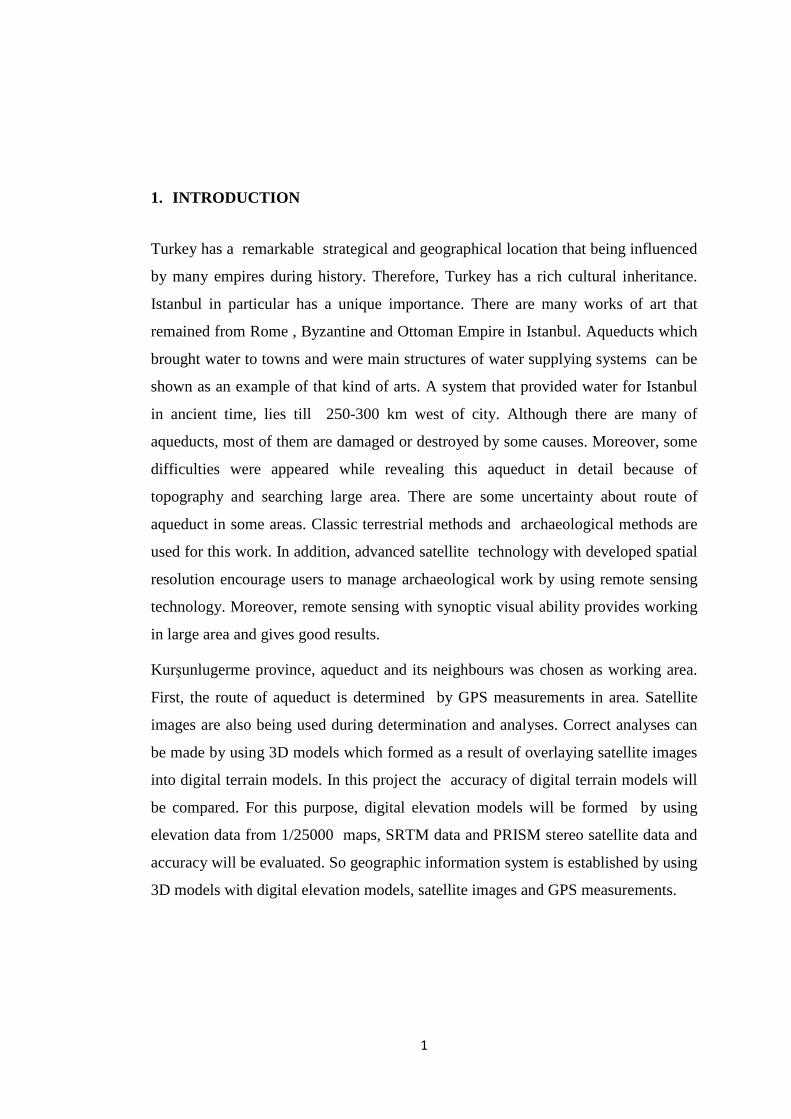
At Hisar, a distinction between archaeological structures and inferred archaeological
structures based on the on the Ikonos-2 satellite image is made (Figure 4. 3). Only
the main visual structures are indicated. The significance of the inferred structures is
not yet clear. Also, colour and shape of these inferred archaeological structures are
less characteristic. The identified objects are remnants of a Byzantine and Early
Hellenistic defence wall and some pre-Roman house constructions (Waelkens et al.,
2000). The perimeter of the inferred defence wall elements that are identified by
visual interpretation amounts to 510 m. The remnants of ancient houses cover an area
of 3800 m2 (De Laet and Paulissen et. al., 2006).
30
Figure 4.3: Visual interpretation of main archaeological structures on IKONOS-2 imagery.
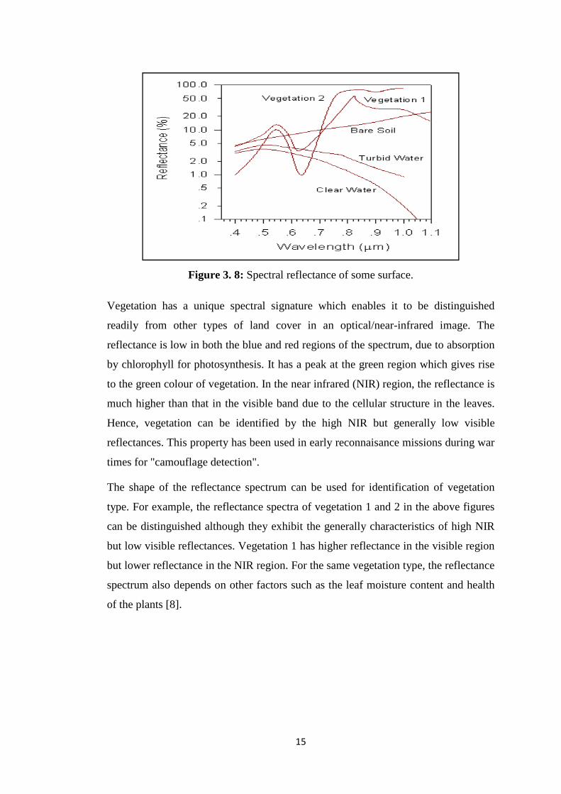
This is a photo of a Gallo-Roman villa that was discovered by aerial survey in 1979,
and is located in an area where Gallo-Roman pottery was located, but the nature and
extent of the site was not evident from the ground (Figure 4. 4). This is considered to
be a large Roman villa, around 100 m per side, and the outline of individual rooms
can be seen. The walls were constructed of cement and stone, and are currently
around 60 cm below the current surface. Individual rooms served as workshops,
granaries, living quarters, as well as many other uses (Source: GIS and Remote
Sensing for Archaeology, Burgundy, France website) [1].
Figure 4.4 : Aerial photo of Gallo-Roman.

31
Much of human history can be traced through the impacts of human actions upon the
environment. The use of remote sensing technology offers the archeologist the
opportunity to detect these impacts which are often invisible to the naked eye. This
information can be used to address issues in human settlement, environmental
interaction, and climate change. Archeologists want to know how ancient people
successfully adapted to their environment and what factors may have led to their
collapse or disappearance. Remote sensing can be used as a methodological
procedure for detecting, inventorying, and prioritizing surface and shallow-depth
archeological information in a rapid, accurate, and quantified manner [6].
32
5. APPLICATIONS
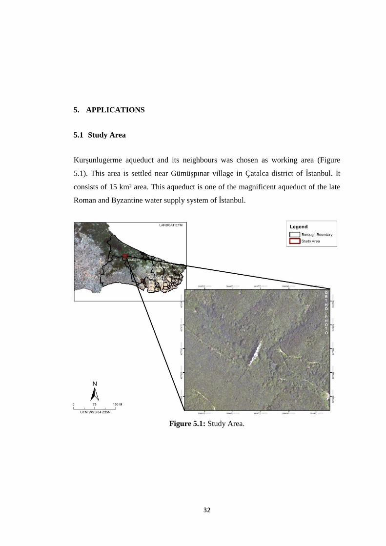
5.1 Study Area
Kurşunlugerme aqueduct and its neighbours was chosen as working area (Figure
5.1). This area is settled near Gümüşpınar village in Çatalca district of Đstanbul. It
consists of 15 km² area. This aqueduct is one of the magnificent aqueduct of the late
Roman and Byzantine water supply system of Đstanbul.
Figure 5.1: Study Area.

33
5.2 Data Used
At this study, IKONOS pansharpened image (2005), LANDSAT ETM (1987) and
orthophoto (2005) are used for visulation, location and overlapping process. To
generate DTM, there are three types images: SRTM (3 arcsecond), 1/25000 scaled
topographical maps and ALOS Prism stereo image (triplet mode, 2.5 m accuracy).
All these data have WGS84 datum and UTM 35N zone projection. Also at this study,
Trimble GeoXT handheld GPS is used. It has horizantal accuracy under 1 meter.
ArcGIS 9.2 (ArcView), ERDAS 9.1 and PCI Geomatica 10.1 (OrthoEngine module)
are used as software.
5.2.1 ALOS
The Advanced Land Observing Satellite (ALOS) developed by the Japan
AerospaceExploration Agency (JAXA) was successfully launched on January 24,
2006. The satellite has three sensors i.e., two optical imagers(PRISM and AVNIR-2)
and an L-band Synthetic Aperture (PALSAR). The mission objectives of ALOS
include cartography, regional observation, and disaster monitoring [10].
The ALOS has three remote-sensing instruments: the Panchromatic Remote-sensing
Instrument for Stereo Mapping (PRISM) for digital elevation mapping, the Advanced
Visible and Near Infrared Radiometer type 2 (AVNIR-2) for precise land coverage
observation, and the Phased Array type L-band Synthetic Aperture Radar (PALSAR)
for day-and-night and all-weather land observation (Figure 5.2). In order to utilize
fully the data obtained by these sensors, the ALOS was designed with two advanced
technologies: the former is the high speed and large capacity mission data handling
technology, and the latter is the precision spacecraft position and attitude
determination capability. They will be essential to high-resolution remote sensing
satellites in the next decade. ALOS have been successfuly launched on an H-IIA
launch vehicle from the Tanegashima Space Center, Japan (Table 5.1) [11].

34
Figure 5. 2: Instruments of ALOS.
Table 5.1: Characteristics of ALOS.
ALOS Characteristics
Launch Date Jan. 24, 2006
Launch Vehicle H-IIA
Launch Site Tanegashima Space Center
Spacecraft Mass Approx. 4 tons
Generated Power Approx. 7 kW (at End of Life)
Design Life 3 -5 years
Orbit
Sun-Synchronous Sub-Recurrent
Repeat Cycle: 46 days Sub Cycle: 2 days
Altitude: 691.65 km (at Equator)
Inclination: 98.16 deg.
Attitude Determination Accuracy
2.0 x 10⁻⁴degree (with GCP)
Position Determination Accuracy
1m (off-line)
Data Rate 240Mbps (via Data Relay Technology Satellite) 120Mbps (Direct Transmission)
Onboard Data Recorder Solid-state data recorder (90Gbytes)

35
5.2.1.1 PRISM The Panchromatic Remote-sensing Instrument for Stereo Mapping (PRISM) is a
panchromatic radiometer with 2.5m spatial resolution at nadir (Figure 5.3). Its
extracted data will provide a highly accurate digital surface model (DSM). PRISM
has three independent optical systems for viewing nadir, forward and backward
producing a stereoscopic image along the satellite's track. Each telescope consists of
three mirrors and several CCD detectors for push-broom scanning. The nadir-
viewing telescope covers a width of 70km; forward and backward telescopes cover
35km each. The telescopes are installed on the sides of the optical bench with precise
temperature control. Forward and backward telescopes are inclined +24 and -24
degrees from nadir to realize a base-to-height ratio of 1.0. PRISM's wide field of
view (FOV) provides three fully overlapped stereo (triplet) images of a 35km width
without mechanical scanning or yaw steering of the satellite (Table 5.2 and 5.3).
Without this wide FOV, forward, nadir, and backward images would not overlap
each other due to the Earth's rotation.
Figure 5. 3: PRISM.

36
Table 5.2: Characteristics of PRISM.
PRISM Characteristics
Number of Bands 1 (Panchromatic)
Wavelength 0.52 to 0.77 micrometers
Number of Optics 3 (Nadir; Forward; Backward)
Base-to-Height ratio 1.0 (between Forward and Backward view)
Spatial Resolution 2.5m (at Nadir)
Swath Width 70km (Nadir only) / 35km (Triplet mode)
S/N >70
MTF >0.2
Number of Detectors 28000 / band (Swath Width 70km) 14000 / band (Swath Width 35km)
Pointing Angle -1.5 to +1.5 degrees (Triplet Mode, Cross-track direction)
Bit Length 8 bits
Table 5.3: Observation modes of PRISM.
Observation Modes
Mode 1 Triplet observation mode using Forward, Nadir, and Backward views (Swath width is 35km)
Mode 2 Nadir (70km) + Backward (35km)
Mode 3 Nadir (70km)
Mode 4 Nadir (35km) + Forward (35km)
Mode 5 Nadir (35km) + Backward (35km)
Mode 6 Forward (35km) + Backward (35km)
Mode 7 Nadir (35km)
Mode 8 Forward (35km)
Mode 9 Backward (35km)
5.2.1.2 AVNIR-2
The Advanced Visible and Near Infrared Radiometer type 2 (AVNIR-2) is a visible
and near infrared radiometer for observing land and coastal zones. It provides better
spatial landcoverage maps and land-use classification maps for monitoring regional

37
environments. AVNIR-2 is a successor to AVNIR that was on board the Advanced
Earth Observing Satellite (ADEOS), which was launched in August 1996. Its
instantaneous field-of-view (IFOV) is the main improvement over AVNIR. AVNIR-
2 also provides 10m spatial resolution images, an improvement over the 16m
resolution of AVNIR in the multi-spectral region. Improved CCD detectors (AVNIR
has 5,000 pixels per CCD; AVNIR-2 7,000 pixels per CCD) and electronics enable
this higher resolution. A cross-track pointing function for prompt observation of
disaster areas is another improvement. The pointing angle of AVNIR-2 is +44 and -
44 degree (Table 5. 4).
Table 5.4: Characteristics of AVNIR-2.
5.2.1.3 PALSAR
The Phased Array type L-band Synthetic Aperture Radar (PALSAR) is an active
microwave sensor using L-band frequency to achieve cloud-free and day-and-night
land observation. It provides higher performance than the JERS-1's synthetic
aperture radar (SAR). Fine resolution in a conventional mode, but PALSAR will
have another advantageous observation mode. ScanSAR, which will enable us to
acquire a 250 to 350km width of SAR images (depending on the number of scans) at
the expense of spatial resolution (Table 5. 5). This swath is three to five times wider
AVNIR-2 Characteristics
Number of Bands 4
Wavelength
Band 1 : 0.42 to 0.50 micrometers Band 2 : 0.52 to 0.60 micrometers Band 3 : 0.61 to 0.69 micrometers Band 4 : 0.76 to 0.89 micrometers
Spatial Resolution 10m (at Nadir)
Swath Width 70km (at Nadir)
S/N >200
MTF Band 1 through 3 : >0.25 Band 4 : >0.20
Number of Detectors 7000/band
Pointing Angle - 44 to + 44 degree
Bit Length 8 bits

38
than conventional SAR images. The development of the PALSAR is a joint project
between JAXA and the Japan Resources Observation System Organization (JAROS).
Table 5. 5: Characteristics of PALSAR.
PALSAR Characteristic
Mode Fine ScanSAR
Polarimetric (Experimental mode)*1
Center Frequency
1270 MHz(L-band)
Chirp Bandwidth
28MHz 14MHz 14MHz,28MHz 14MHz
Polarization HH or VV
HH+HV or VV+VH
HH or VV HH+HV+VH+VV
Incident angle
8 to 60deg.
8 to 60deg.
18 to 43deg. 8 to 30deg.
Range Resolution
7 to 44m 14 to 88m
100m (multi look)
24 to 89m
Observation Swath
40 to 70km
40 to 70km
250 to 350km 20 to 65km
Bit Length 5 bits 5 bits 5 bits 3 or 5bits
Data rate 240Mbps 240Mbps 120Mbps,240Mbps 240Mbps
NE sigma zero *2
< -23dB (Swath Width 70km) < -25dB (Swath Width 60km)
< -25dB < -29dB
S/A *2,*3
> 16dB (Swath Width 70km) > 21dB (Swath Width 60km)
> 21dB > 19dB
Radiometric accuracy
scene: 1dB / orbit: 1.5 dB

39
5.3 Methods Used
5.3.1 Digital Terrain Model (DTM)
A Digital Elevation Model (DEM) is a digital representation of ground surface topography or terrain. It is also widely known as a digital terrain model (DTM). A DEM can be represented as a raster (a grid of squares) or as a triangular irregular network. DEMs are commonly built using remote sensing techniques, however, they may also be built from land surveying. DEMs are used often in geographic information systems, and are the most common basis for digitally-produced relief maps. By using benefits of DTM, we are able to obtain slope maps, aspect maps and various profiles (longitudinal and transverse sections of valleys, etc).
Digital elevation models may be prepared in a number of ways, but they are frequently obtained by remote sensing rather than direct survey. One powerful technique for generating digital elevation models is interferometric synthetic aperture radar; two passes of a radar satellite (such as RADARSAT-1) suffice to generate a digital elevation map tens of kilometers on a side with a resolution of around ten meters. One also obtains an image of the surface cover.
Another powerful technique for generating a Digital Elevation Model is using the Digital image correlation method. It implies two optical images acquired with different angles taken from the same pass of an airplane or an Earth Observation satellite (such as the HRS intrument of SPOT5).
Older methods of generating DEMs often involve interpolating digital contour maps that may have been produced by direct survey of the land surface; this method is still used in mountain areas, where interferometry is not always satisfactory. Note that the contour data or any other sampled elevation datasets (by GPS or ground survey) are not DEMs, but may be considered Digital terrain models. A DEM implies that elevation is available continuously at each location in the study area.
Older methods of generating DEMs often involve interpolating digital contour maps
that may have been produced by direct survey of the land surface; this method is still
used in mountain areas, where interferometry is not always satisfactory. Note that the
contour data or any other sampled elevation datasets (by GPS or ground survey) are
not DEMs, but may be considered Digital terrain models. A DEM implies that
elevation is available continuously at each location in the study area.
5.3.2 DTM Generation From Topographical Maps
DTMs can be obtained by using different methods such as stereoscope satellite
images and land readings. Having been used as the basis of this study, the 1/25000

40
scaled topographic maps were digitised by using 10 m contour line intervals. First
the irregular Triangle Network (TIN) was generated from the contour line curves and
altitude points using the 3D Analyst module. All points in this data structure are
generally interconnected via Delaunal triangulation, which combines the centres of
adjacent thiessen polygons (Kumler, 1994). The TIN model is then converted into
raster format and DTM is generated accordingly. The grid size of this conversion
was 10 m. Selection of this value was affected by the use of contour lines at either 10
m or 5 m intervals. Having been created from contour lines, the DTMs with small
intervals feature higher altimetry accuracy and constitute useful data resources
(Wilson and Gallant, 2000). The 3D model was created by using the generated DTM
(Figure 5.5). The DTM was also used to create the Hillshade 3D model (Figure 5.4)
(Akar, 2008).
Figure 5.4: Hillshade model. Figure 5.5: DTM.
5.3.3 DTM Generation From Stereo Images
Actual very high resolution (VHR) satellite image data with resolution of about one
meter offer the possibility to see many details in urban areas. Objects like houses,
trees and cars can be interpreted easily with visual methods, while the automatic
interpretation of this kind of space borne data is still a very busy field of research.
Especially, an automatic DTM generation from along track stereo pairs of VHR
optical data from space, like IKONOS or Quick Bird images, offer new challenges
for developing techniques for the automatic interpretation of homologous image
structures and further for object extraction (Figure 5.6). So, at present a primary
target in city modelling is the quest for algorithms creating fully automatically good
and reliable digital elevation models from relatively easy to acquire high resolution
stereo satellite imagery [1, 2] [12].
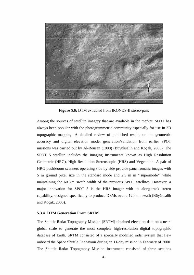
41
Figure 5.6: DTM extracted from IKONOS-II stereo-pair.
Among the sources of satellite imagery that are available in the market, SPOT has
always been popular with the photogrammetric community especially for use in 3D
topographic mapping. A detailed review of published results on the geometric
accuracy and digital elevation model generation/validation from earlier SPOT
missions was carried out by Al-Rousan (1998) (Büyüksalih and Koçak, 2005). The
SPOT 5 satellite includes the imaging instruments known as High Resolution
Geometric (HRG), High Resolution Stereoscopic (HRS) and Vegetation. A pair of
HRG pushbroom scanners operating side by side provide panchromatic images with
5 m ground pixel size in the standard mode and 2.5 m in ‘‘supermode’’ while
maintaining the 60 km swath width of the previous SPOT satellites. However, a
major innovation for SPOT 5 is the HRS imager with its along-track stereo
capability, designed specifically to produce DEMs over a 120 km swath (Büyüksalih
and Koçak, 2005).
5.3.4 DTM Generation From SRTM
The Shuttle Radar Topography Mission (SRTM) obtained elevation data on a near-
global scale to generate the most complete high-resolution digital topographic
database of Earth. SRTM consisted of a specially modified radar system that flew
onboard the Space Shuttle Endeavour during an 11-day mission in February of 2000.
The Shuttle Radar Topography Mission instrument consisted of three sections

42
(Figure 5. 7). The main antenna was located in the payload bay of Space Shuttle
Endeavour, the mast was connected to the main antenna truss, and an outboard
antenna was connected to the end of the mast.
Figure 5. 7: SRTM Instrument.
In order to gather topographic (elevation) data of Earth's surface, SRTM used the
technique of interferometry. In interferometry, two images are taken from different
vantage points of the same area. The slight difference in the two images allows
scientists to determine the height of the surface.
The main antenna actually consisted of two antennas and the avionics that computed
the position of the antennas. Each antenna was made up of special panels that could
transmit and receive radar signals. One antenna was called the C-band antenna and
could transmit and receive radar wavelenths that are 5.6 centimeters long. During the
mission the C-band radar, with a swath width (width of the radar beam on Earth's
surface) of 225 kilometers, scanned about 80% of the land surface of the Earth.
The other antenna was the X-band antenna. This antenna could transmit and receive
radar wavelenths that are 3 centimeters long. The X-band radar, with a swath width
of 50 kilometers, will produce topographic maps at a somewhat higher resolution
than the C-band data, but will not have near-global coverage (Figure 5.8) [13].

43
Figure 5.8: Main antenna of SRTM.
Digital elevation models (DEMs) are a basic component of any geoinformation
system (GIS). The terrain cannot only be described by the horizontal components;
the height belongs to complete information. In addition height models are required
for the generation of orthoimages – one of the most often used photogrammetric
product. DEMs can be generated by laser scanning, photogrammetric methods or
interferometric synthetic aperture radar (InSAR). In any case it is time consuming
and expensive. The worldwide lack of qualified and accessible DEMs has been
improved with the Shuttle Radar Topography Mission (SRTM) in February 2000.
Based on InSAR height models have been generated covering the world from 56°
southern up to 60.25° northern latitude. The DEMs based on the US C-band are
available free of charge on the internet with a spacing of 3 arcsec, corresponding to
approximately 92m at the equator. Only for the USA data with a spacing of 1 arcsec
(~ 30m) are also in the WEB. The DEMs based on the German / Italian X-band can
be ordered from the DLR, Germany with a spacing of 1 arcsec. But without
scanSAR-mode the X-band DEM has large gaps between the swaths of 45km width.
The nearly worldwide and free of charge available SRTM C-band height models are
an important component of the knowledge about our spatial environment (Figure 5.
9). The homogenous accuracy is sufficient for several applications and for wide areas
of the world it is more detailed information about the surface than known before
[14].

44
Figure 5.9: DEM generation from SRTM data.
5.4 Methodology
5.4.1 DTM Generation From Topographical Maps
1/25000 scaled topographic maps were digitised by using 10 m contour line intervals
(Figure 5.10). First the Triangle irregular Network (TIN) ((Figure 5.11) was
generated from the contour line curves and altitude points using the 3D Analyst
module. All points in this data structure are generally interconnected via Delaunal
triangulation. The TIN model is then converted into raster format and DTM is
generated accordingly (Figure 5. 12). The grid size of this conversion was 10 m.
Also, DTM of study area and overlapping of IKONOS image on this DTM are
shown below (Figure 5. 13).
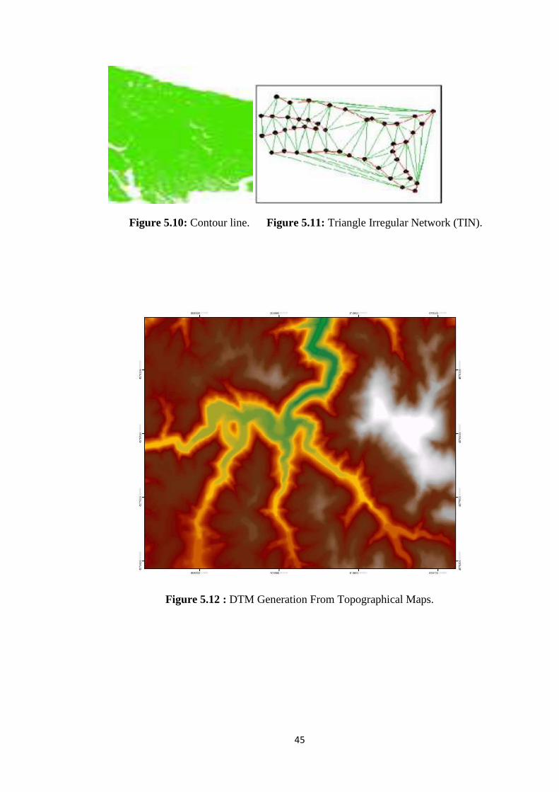
45
Figure 5.10: Contour line. Figure 5.11: Triangle Irregular Network (TIN).
Figure 5.12 : DTM Generation From Topographical Maps.

46
Figure 5.13 :Overlapping of IKONS Image on DTM Generated Topographical Maps
5.4.2 DTM Generation From SRTM
The DEMs based on the US C-band are available free of charge on the internet with
a spacing of 3 arcsec, corresponding to approximately 92 m at the equator.
Figure 5.14 : DTM Generation From SRTM.

47
Also, DTM of study area and overlapping of IKONOS image on this DTM are
shown below (Figure 5.14 and 5.15).
Figure 5.15 : Overlapping of IKONOS Image on DTM Generated from SRTM.
5.4.3 DTM Generation From Stereo Images
To generate DTM, ALOS Prism stereo images (triplet mode ) are used (Figure 5.16) .
This data has georeferenced, nearest neighbour, UTM projection. Also it has level
1B2. At this study, backward and nadir images were selected to generate DTM. Their
swath area consist of 35 km².

48
Figure 5.16 : ALOS Prism Image.
Firstly, a new project was created with using OrthoEngine module (Figure 5.17).
Then Project information was selected. The next step was to define the projection
(Figure 5.18). It was entered in the appropriate projection information for the PRISM
dataset. It was recommended that we use “Set GCP Projection based on Output
Projection” option for the GCP projection.

49
Figure 5.17 : Project Information.
Figure 5.18 : Projection Information.

50
Secondly, it was aimed import PRISM imagery into project. The dataset shows
stereo imagery from a single PRISM CCD, there are two types of files. One type is
prefixed with the term “IMG” and the other type is prefixed with the term “VOL”.
The “VOL” files simply maintain information about the dataset, such as the images
included in the dataset, their associated channel, and filename. The “IMG” files are
the actual images in each dataset. Note that both file types end with either “_N” or
“_B”. N indicates nadir view, and B indicates backward view. Therefore, “VOL”
files ending in “_B” maintain information about the backward view dataset, and
“VOL” files ending in “_N” maintain information about the nadir view dataset.
To begin importing the PRISM imagery into project:
• Orthoengine select “Data Input” from the processing step, and Click “Read
CD- ROM data”( Figure 5.19).
• In the Read CD-ROM data window, select “PRISM (LGSOWG)”.
• Select the CD header filename (the VOLUME file).
• Select the channel to import. For example, if the imagery provided is prefixed by
“IMG-05” then this would indicate that the channel is 5.
• Once the channel is selected, provide an appropriate PCIDSK filename and click
READ.
• Repeat this procedure for all images in both the nadir and backward views.

51
Figure 5.19 : Data Input.
Figure 5.20 : Format Changing.
Thirdly, once the imagery has been imported into PIX format, opened a stereo pair
(Figure 5.20) . In the processing step drop down in Orthoengine, selected “GCP/TP
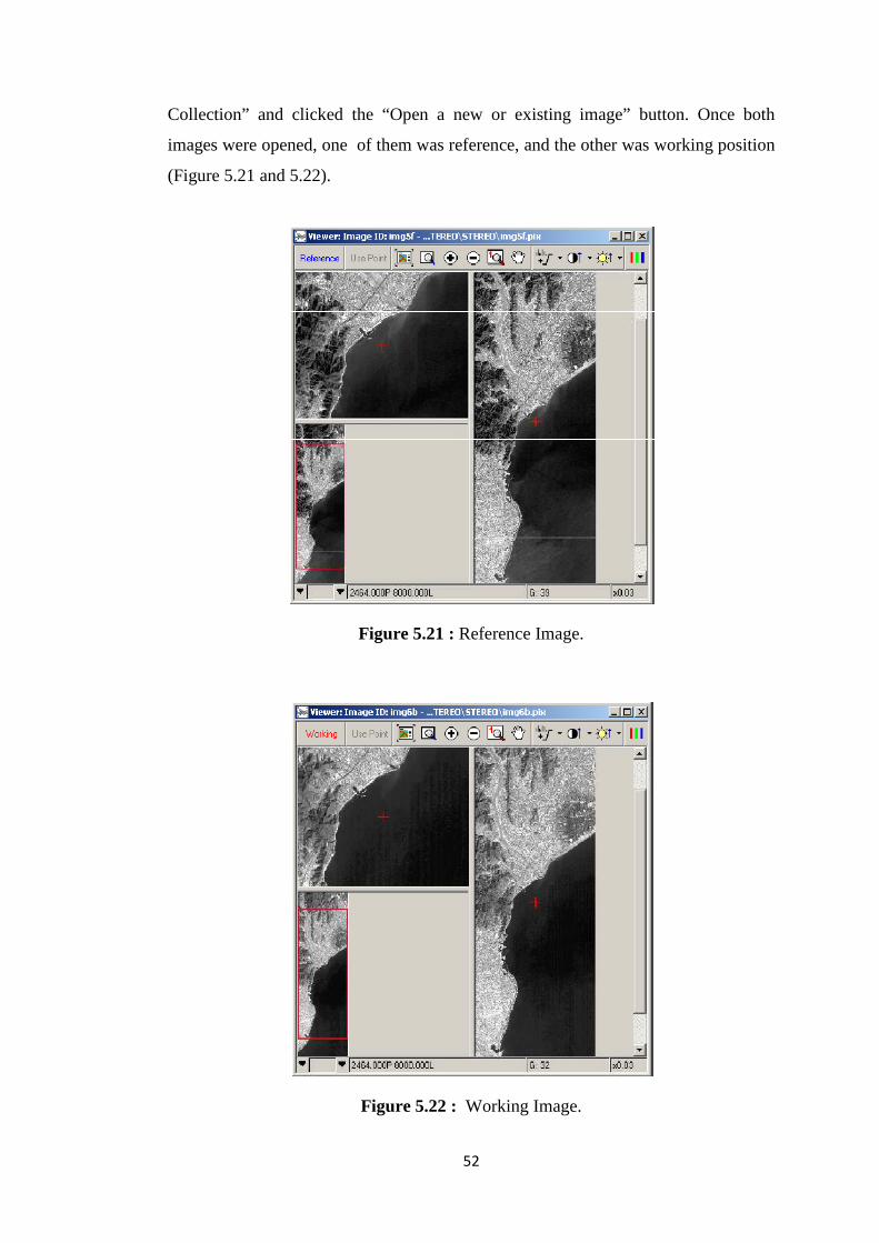
52
Collection” and clicked the “Open a new or existing image” button. Once both
images were opened, one of them was reference, and the other was working position
(Figure 5.21 and 5.22).
Figure 5.21 : Reference Image.
Figure 5.22 : Working Image.

53
The next step was collection of stereo GCPs. Now that the images have been opened,
it’s time to start collecting Stereo GCPs. Stereo GCPs are GCPs that are present in
both images. These are advantageous for several reasons. Firstly, Stereo GCPs are
useful because they can be used to derive elevation information from a stereo dataset.
This is the result of the parallax difference which occurs between the stereo pair.
Secondly, Stereo GCPs are heavily weighted in the adjustment model. It is important
when collecting Stereo GCPs that the user take the utmost care to ensure that
accurate and precise Stereo GCPs are chosen.
• Selected the first image we would like to collect a GCP in by setting it to the
working image. The working image chosen for this example is the nadir view image.
• In the working image viewer, located a clearly identifiable point we would like to
use as a GCP and click “Use Point”.
• To ensure better results, make sure that the GCP we choose is a well defined
location in our image (such as an intersection of two roads). Also ensure that the
GCP is identifiable in both images in the stereo pair, and the control source image.
• Notice that after we clicked “Use Point” the GCP Collection Window updates with
the pixel and line location of the GCP (Figure 5.23).
• Then located the same location (in this case, G0001) in the geocoded image. Be
sure to get as close as possible to the same location as that in our working image.
Figure 5.23 : Selection of GCP.
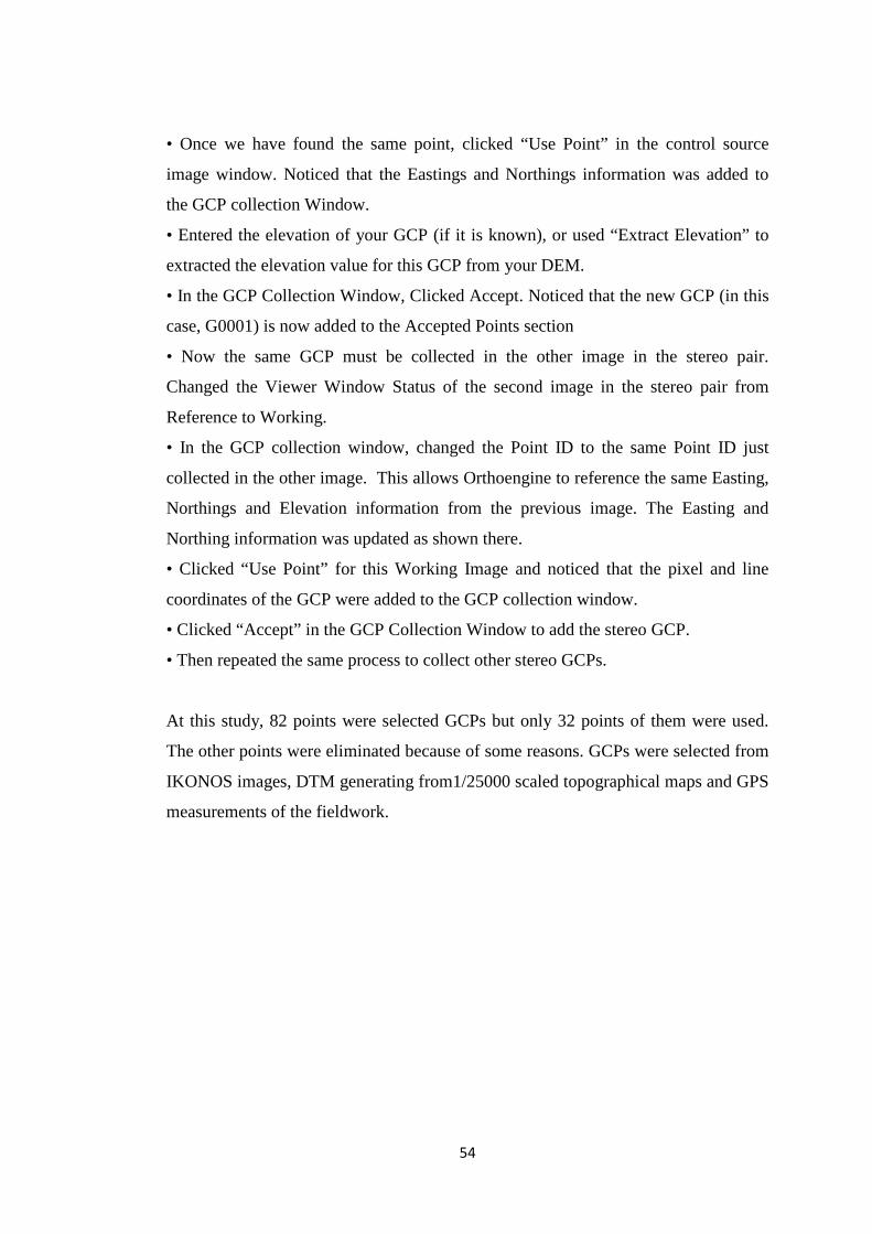
54
• Once we have found the same point, clicked “Use Point” in the control source
image window. Noticed that the Eastings and Northings information was added to
the GCP collection Window.
• Entered the elevation of your GCP (if it is known), or used “Extract Elevation” to
extracted the elevation value for this GCP from your DEM.
• In the GCP Collection Window, Clicked Accept. Noticed that the new GCP (in this
case, G0001) is now added to the Accepted Points section
• Now the same GCP must be collected in the other image in the stereo pair.
Changed the Viewer Window Status of the second image in the stereo pair from
Reference to Working.
• In the GCP collection window, changed the Point ID to the same Point ID just
collected in the other image. This allows Orthoengine to reference the same Easting,
Northings and Elevation information from the previous image. The Easting and
Northing information was updated as shown there.
• Clicked “Use Point” for this Working Image and noticed that the pixel and line
coordinates of the GCP were added to the GCP collection window.
• Clicked “Accept” in the GCP Collection Window to add the stereo GCP.
• Then repeated the same process to collect other stereo GCPs.
At this study, 82 points were selected GCPs but only 32 points of them were used.
The other points were eliminated because of some reasons. GCPs were selected from
IKONOS images, DTM generating from1/25000 scaled topographical maps and GPS
measurements of the fieldwork.

55
Figure 5.24 : All Grand Control Points.
After that, all GCPs have been collected, switched to “Model Calculations” in the
processing step of Orthoengine and clicked the “ Compute Model” buton (Figure
5.24).
Figure 5.25 : RMS Value.

56
After model calculation, RMS value was calculated as 0.6 (Figure 5.25).
Finally, to extract DTM from stereo:
• In Orthoengine, switched to the “DEM From Stereo” option in the processing step.
Then clicked the “Create Epipolar Image” button. The generate epipolar images
window appears (Figure 5.26).
• In the generate epipolar images window, selected a left image and right image.
Then clicked add epipolars to table. The epipolar pairs were then added to the
epipolar pairs table. For this example, it was used a down sample factor of 2.
• Then clicked generate pairs to generate the epipolar images. (This may take some
time depending on file size).
• Now that the epipolar pairs have been generated,
clicked the “Extract DEM automatically” button in Orthoengine
Figure 5.26 : Generating Epipolar Image.

57
• In the Automatic DEM extraction window, put a checkmark next to the stereo pair
we were working with and set a pixel sampling interval of 1. Selected the option
“Create Geocoded DEM” and choose an output filename for the DEM.
Figure 5.27 : Automatic DEM Extraction.
After clicked Extract DEM, the result was acquired successfully (Figure 5.27). Also,
DTM of study area and overlapping of IKONOS image on this DTM are shown
below.

58
Figure 5.28 : DTM Generated From Prism Image.
Figure 5.29 : Study Area of DTM Generated From Prism Image.

59
Figure 5.30 :Overlapping of IKONOS Image on DTM Generated From Prism Image
5.4.4 Generation And Using GIS
At this study, ArcGIS 9.2 was selected and used as a geographic information system
software. Satellite data, GPS points and three DTM’s which were generated from
different resources were added as layers (Figure 5.31). Morever, overlapping of
IKONOS image on DTM generated from SRTM, stereo images and topographical
maps was composed. At the end of ongoing Tübitak project, all data (hydrological,
archaeological, and others) will have been added to this system. So, some processes
like inquiry and analysis will be available using GIS.
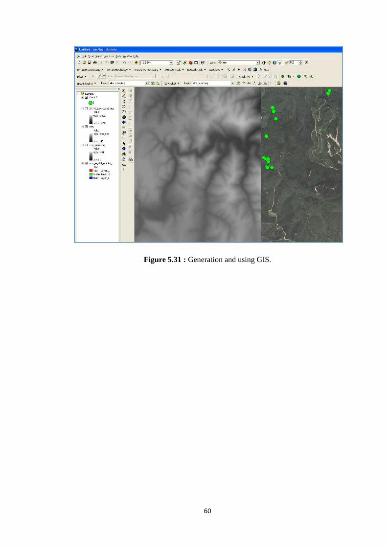
60
Figure 5.31 : Generation and using GIS.

61
6. RESULTS
Improvements at satellite technologies and information systems has caused the
frequently usage of remote sensing and integration of geographic information system
in archaeological applications. Đstanbul has a remarkable strategical and
geographical location that being influenced by many empires during history.
Therefore, it has a rich cultural inheritance. At this study, Kurşunlugerme aqueduct
in Çatalca District of Đstanbul has been the important part of water supply system at
the time of Roman, Byzantine and Otoman Empires, and its environment has been
chosen. Three types of DTM were generated from different resources. When we
compare two DTM (1/25000 topographical maps and ALOS Prism stereo images),
they have nearly same accuracy values. The other DTM generating from SRTM has
lower accuracy ( 6-7 meters) than the others. If it has been taken better accuracy
GCPs in DTM generating from Prism stereo images, the result would be more
precise and reliable. The three dimensional model, which can get by overlapping
satellite images onto regional digital terrain models, can provide the terrain
topography to demonstrate. Vital analyses and comments may make by adding GPS
measurements at archaeological structures at study area. In conclusion, these
archaeological structures should be preserved with using GIS and remote sensing
technologies.
62
REFERENCES
Akar, Đ., 2008, Application of GIS and Remote Sensing Generating in 3D Modeling
and Determination of morphological Features with in “Ağrı Volcano” Ağrı, Turkey.
Allen, Kathleen M.S., Stanton W. Green and Ezra B.W. Zubrow. 1990.
Interpreting Space: GIS and Archaeology. Taylor and Francis, London.
Büyüksalih, G., Koçak, G., Topan, H., Oruç, M., Marangoz, A., 2005, SPOT
Revisited: Accuracy Assessment, DEM Generation and Validation from Stereo
SPOT 5 HRG Images, Photogrammetric Record, 20(110), 1-18 (2005).
Campbell, J.B. (2002), Introduction to Remote Sensing, 3rd ed., The Guilford Press,
New York, NY Clark et al., 1998 C.D. Clark, S.M. Garrod and M.P. Pearson,
Landscape archaeology and remote sensing in southern Madagascar, International
Journal of Remote Sensing 19 (1998) (8), pp. 1461–1477.
Chandra, A. M., Ghosh S. K., 2006, Remote Sensing and Geographical Information
System, pp. 145 – 154.
Changlin, W., Ning, Y., Yueping, N., Lin, Y., 2004. Environmental Study and
Information Extraction of Archaeological Features with Remote Sensing Imagery in
Arid Area of Western China, Proceedings of the International Conference on Remote
Sensing Archaeology, Beijing.
Emmolo, D., Franco, V., Lo Brutto, M., Orlando, P., Villa, B., 2004.
Hyperspectral Techniques and GIS for Arechaeological Investigation, Proceedings of
the XXth ISPRS congress on Geo-imagery Bridging Continents, Istanbul, Turkey.
Jensen, J. R. 2000, Remote Sensing of the Environment: An Earth Resource
Perspective. Prentice Hall: New York.

63
Kumler, Mark P. (1994) “An Intensive Comparison of Triangulated Irregular
Networks (TINs) and Digital Elevation Models (DEMs)”. Cartographica. Vol. 32,
No. 2. Monography 45.
PCI Geomatics, 1998 PCI Geomatics, OrthoEngine reference manual, PCI
Geomatics, Ontario (1998).
P.J. Gibson, 2000, Introductory Remote Sensing, Princicles and Concepts, Routledg. Renfrew, C., Bahn, P., 2000, Archaeology: Theories, Methods, and Practice. Third
edition. New York: Thames and Hudson.
Sever, T.L., 1995 Sever, Remote Sensing. In: P.E. McGovern, T.L. Sever, J.W.
Myers, E.E. Myers, B. Bevan, N.F. Miller, S. Bottema, H. Hongo, R.H. Meadow, P.I.
Kuniholm, S.G.E Bowman, M.N. Leese, R.E.M. Hedges, F.R. Matson, I.C.
Freestone, S.J. Vaughan, J. Henderson, P.B. Vandiver, C.S. Tumosa, C.W. Beck, P.
Smith, A.M. Child, A.M. Pollard, I. Thuesen and C. Sease, Editors, Science in
Archaeology, American Journal of Archaeology 99 (1995) (1), pp. 83–84.
V. De Laet, E. Paulissen, M. Waelkens (2007). “Methods for the extraction of
archaeological features from very high resolution Ikonos-2 remote sensing imagery,
Hisar (southwest Turkey).” Journal of Archaeological Science 34(5): 830-841 (SCI:
1.316).
M. Waelkens, H. Vanhaverbeke, E. Paulissen, J. Poblome, J. Reyniers, W.
Viane, J. Deckers, B. Decupere, W. Van Neer, H.A. Ekinci and M.O. Erbay, The
1996 and 1997 survey season at Sagalassos. In: M. Waelkens and L. Loots, Editors,
Sagalassos V, Report on the Survey and Excavation Campaigns of 1996 and 1997,
Acta Archaeologica Lovaniensia Monographiae 11A, Leuven University Press,
Leuven (2000), pp. 17–216.
Wilson JP, Gallant JC (2000) Terrain analysis: principles and applications. John
Wiley and Sons, Inc.: New York.
Wüst, T., Nebiker, S. und Landolt, R., 2004. Applying The 3D DIS DILAS to
Archaeology and Cultural Heritage Projects – Requirements and First Results, XX
ISPRS Congress. International Archives of Photogrammetry, Remote Sensing and
Spatial Information Sciences, Vol. XXXV-B5, Istanbul, Turkey.

64
[1] http://en.wikipedia.org/wiki/Archaeology
[2] http:// www.arkeoloji.web.tr
[3] http://www.gisdevelopment.net/application/archaeology/general
[4] http://www.geographymatters.com/industries/archaeology/
[5] http://www.pop.psu.edu/gia-core/pdfs/gis_rd_02-32.pdf
[6] http://www.ghccc.msfc.nasa.gov/archaeology
[7] http://www.ccrs.nrcan.gc.ca/resource/tutor/fundam/index_e.php
[8] http://www.crisp.nus.edu.sg/~research/
[9] http://www.csc.noaa.gov/product/nchaz
[10] http://www.geoimage.com.au/geoweb/pdfs/flyers/ALOS_flyer.pdf
[11] http://www.eorc.jaxa.jp/ALOS/
[12] http://www.isprs.org/commission8/workshop_urban/krauss.pdf
[13] www2.jpl.nasa.gov/srtm
[14] http://www.geoconnexion.com/
[15] http://www.3darchaeology.org

65
CURRICULUM VITAE
He was born in Salihli in 1981. He was graduated from Dadağlı primary school and Salihli high school. He began to study bachelor programme of Geodesy and Photogrammetry Engineering in Istanbul Technical University (ITU) in 2000. He was graduated in 2005. He has been studying for his master programme in Geomatics Engineering in Institute of Science and Technology since 2005.