Department of Agricultural and Resource Economics

The University of Maryland, College Park

Dual Approaches to the Analysis of

Risk Aversion

by

Robert G. Chambers and John Quiggin

WP 02-04

DUAL APPROACHES TO THE ANALYSIS OF RISK AVERSION

Robert G. Chambers Professor of Agricultural and Resource Economics, University of Maryland

Adjunct Professor of Agricultural and Resource Economics, University of Western Australia rchambers@arec.umd.edu

John Quiggin

Australian Research Council Senior Fellow, Australian National University

May 2002 Copyright 8 2002 by Robert G. Chambers and John Quiggin All rights reserved. Readers may make verbatim copies of this document for non-commercial purposes by any means, provided that this copyright notice appears on all such copies.

Dual Approaches to the Analysis of Risk Aversion

Robert G. Chambers and John Quiggin

May 15, 2002

DUAL APPROACHES TO THE ANALYSIS OF RISK AVERSION

A series of classic papers (Yaari, 1965; Yaari, 1969; Peleg and Yaari, 1975) observe

that choice under uncertainty is formally equivalent to choice over commodity bundles in

conventional consumer theory. Although this is an old observation, its implications are yet

to be fully exploited. Using dual concepts familiar from standard producer-consumer theory,

this paper presents a systematic analysis of preferences over uncertain outcomes in terms of

convex sets and their supporting hyperplanes. The aim is to extend the insights of Peleg

and Yaari in the light of the dual approaches developed since their work was published.

The analysis commences by representing convex preference sets over uncertain outcomes

in terms of the translation function, originally developed in the theories of inequality mea-

surement and consumer preferences under certainty (Blackorby and Donaldson, 1980; Luen-

berger, 1992), and its concave conjugate, which we refer to as the expected-value function.

Subjective probabilities are interpreted as normalized supporting hyperplanes in the neigh-

borhood of the sure thing, and more generally, for risk-averse individuals, marginal rates

of substitution between state-contingent incomes are interpreted as relative risk-neutral

probabilities.

We next consider the notion of risk aversion, beginning with Yaaris (1969) concept of

risk aversion. A dual deÞnition of risk aversion with respect to a probability vector is then

offered. This dual deÞnition of risk aversion gives rise to dual versions of the PrattArrow

absolute and relative risk premiums as functions of the probabilities. For an individual

risk-averse with respect to a given probability vector, these dual risk premiums take their

maximum values (zero and one) at that vector, just as the corresponding primal measures

are minimized at certainty.

The paper then examines the concepts of constant absolute risk aversion (CARA), con-

stant relative risk aversion (CRRA), and linear risk tolerance (LRT) in a dual framework.

These concepts are interpreted as homotheticity properties, and each is shown to be charac-

terized by an invariance property of the risk-neutral probabilities. Homotheticity conditions

of various kinds play a central role in consumer and producer theory. However, relatively

little attention has been given to these properties for preferences over uncertain outcomes.

We illustrate the power of the dual approach in analyzing preferences over uncertain out-

1

comes by showing that linear risk tolerance is simply characterized as quasi-homotheticity.

And, even though for general quasi-concave LRT preferences, there typically do not exist

closed-form preference functionals, the dual formulation offers a simple characterization.

Next, a dual analysis of the class of constant risk averse preferences studied by Safra

and Segal (1998) is provided. The associated expected-value function is derived and shown

to imply that the the only quasi-concave preference structures belonging to this class are

the maxmin expected value (MMEV) preferences identiÞed by Safra and Segal (1998). Our

demonstration in terms of risk-neutral probabilities and the expected-value function leads

to the further observation that the plunging behavior observed by Yaari (1987) for his dual

preference structure is characteristic of the entire class of constant-risk-averse, quasi-concave

preferences. Finally, our methods are applied to a generic convex choice problem. Equilib-

rium conditions for such problems are characterized by a preference analogue to the Peleg

Yaari (1975) efficient set result, and comparative static results for LRT and constant risk

averse preferences are presented. The Þnal section concludes.

1 Notation and Basic Concepts

For a proper concave function f : <S → <, its superdifferential at x is the closed, convex

set:

(1) ∂f (x) =©

v ∈<S : f (x) + v (z− x) ≥ f (z) for all zª.

The elements of ∂f (x) are referred to as supergradients. If f is differentiable at x, ∂f (x) is

a singleton. If ∂f (x) is a singleton, f is differentiable at x (Rockafellar, 1970). ∂+

∂xdenotes

the right-hand partial derivative with respect to x.

We consider preferences over random variables represented as mappings from a state

space Ω to an outcome space Y ⊆ <. We refer to the outcomes as income. Our focus is onthe case where Ω is a Þnite set 1, ...S, and the space of random variables is Y S ⊆ <S. Theunit vector is denoted 1 = (1, 1, ...1), and P ⊂ <S++ denotes the probability simplex. DeÞneei as the i-th row of the S × S identity matrix , ei = (0, ..., 1, 0, ..., 0) .

Preferences over state-contingent incomes are given by an ordinal mappingW : <S → <.W is continuous, nondecreasing, and quasi-concave in y. Quasi-concavity ensures that the

2

least-as-good sets of the preference mapping

V (w) = y :W (y) ≥ w

are convex, and that the individual is averse to risk in the sense of Yaari (1969).

2 The Translation Function and the Expected-Value

Function

The translation function, B : <× Y S → <, is deÞned:

B(w,y; 1) = maxβ ∈ < : y − β1 ∈ V (w)

if y − β1 ∈ V (w) for some β, and −∞ otherwise (Blackorby and Donaldson, 1980; Lu-

enberger, 1992).1 The properties of B(w,y; 1) are well known (Blackorby and Donaldson,

1980; Luenberger, 1992; Chambers, Chung, and Färe, 1996), and are summarized for later

use in the following lemma:

Lemma 1 B(w,y;1) satisÞes:

a) B(w,y;1) is nonincreasing in w and nondecreasing and concave in y;

b) B(w,y + α1;1) = B(w,y; 1) + α, α ∈ < (the translation property);c) B(w,y;1) ≥ 0⇔ y ∈ V (w);d) B(w,y; 1) is jointly continuous in y and w in the interior of the region <×Y S where

B(w,y; 1) is Þnite.

An important special case is the certainty-equivalent representation of preferences,

e (y) = −B (W (y) ,0; 1) .

Because the preference functional is ordinal, no loss of generality is involved in replacing

W (y) by its ordinal transform e (y) , and in what follows we always do so, writing B (e,y; 1)

in place of B (w,y;1) .1The translation function is a special case of the beneÞt function deÞned by Luenberger (1992).

3

We refer to the concave conjugate of the translation function, B (e,y; 1) , as the expected-

value function E : P × <→ <. It is deÞned by

E (π,e) = infyπy−B (e,y;1) π ∈P .

Chambers (2001) shows that, as a consequence of Lemma 1.b, if y (π, e) ∈ arg inf πy−B (e,y; 1) ,then y (π, e) + δ1 ∈ arg inf πy−B (e,y; 1) for δ ∈ <. This indeterminancy in the optimiz-ing set can be resolved by a convenient normalization. Because, for π ∈P, πy−B (e,y;1) =π [y−B (e,y; 1)1] , and because Lemma 1.c impliesB (e,y−B (e,y; 1) 1; 1)≥0,the expected-value function is equivalently expressed as:

E (π,e) = infyπy :B (e,y; 1) ≥ 0 π ∈P

= infyπy : y ∈V (e)

if there exists some y ∈V (e) , and ∞ otherwise. Hence, the expected-value function has an

alternative interpretation as the expenditure function for V (e) in the state-claim prices π.

If V (e) is nonempty, B (e,y; 1) is a continuous and nondecreasing proper concave func-

tion, and thus E (π,e) is a closed, proper concave2 function nondecreasing on P (Theorem

12.2, Rockafellar, 1970). It is also continuous and nondecreasing in e in the region where it

is Þnite. And because e (e1) = e, E (π,e) ≤ e.Figure 1 illustrates the relationship between the expected value function and the certainty

equivalent. Because the expected-value function is an expenditure function, in terms of the

ArrowDebreu state-claim prices π, the difference between e (y) and E (π,e) thus measures

the cost savings in achieving e that can be realized by operating in a complete ArrowDebreu

contingent claims economy at state-claims prices π.

By basic results on conjugate duality (Theorem 12.2, Rockafellar, 1970), the translation

function can be reconstructed from the expected-value function by applying the following

conjugacy relationship

B (e,y;1) = infπ∈P

πy−E (π,e) .2A concave function, g (x) , is proper if there is at least one x such that g (x) > −∞, and g (x) < ∞ for

all x. A concave function is closed if and only if it is upper semi-continuous (Rockafellar, 1970, p. 52).

4

A well-known implication of the conjugacy of the translation function and the expected-value

function (Corollary 23.5.1, Rockafellar, 1970) is

(2) π ∈ ∂B (e,y;1)⇐⇒ y ∈ ∂E (π, e)

in the relative interior of their domains.3 Expression (2) is a general statement of Shephards

Lemma, familiar from standard consumer and producer theory, for superdifferentiable struc-

tures. More formally, by (2) in the interior of their domains

y (π, e) ∈ arg inf πy−B (e,y; 1)⇒ y (π, e) ∈ ∂E (π, e) ,

because

πy (π, e)− B (e,y (π, e) ;1) ≤ πy−B (e,y; 1) , for all y

⇓π ∈ ∂B (e,y (π, e) ;1)

⇓y (π, e) ∈ ∂E (π, e) ,

where the Þrst ⇒ follows by the deÞnition of the superdifferential, and the second by (2).

By a parallel argument, p (e,y) ∈ arg inf πy−E (π,e) ⇒ p (e,y) ∈ ∂B (e,y; 1) . Thus,the supergradients of the translation function are interpretable as compensated state-claim-

price-dependent demand functions for the state-claim vector y.

2.1 Risk-neutral probabilities

Because the translation function and the expected-value function form a conjugate pair, they

offer a natural method for deÞning and generating subjective notions of probability in terms

of their superdifferentials. Because there is no requirement for smoothness, this allows for

the analysis of both Þrst-order and second-order risk aversion, which has proven central in

the generalized expected utility literature (Epstein and Zinn 1990; Segal and Spivak 1990;

Machina, 2001).3Here, as elsewhere in the paper, these are understood to be the superdifferential of B in terms of y and

the superdifferential of E in terms of π.

5

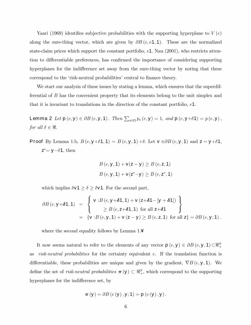
Yaari (1969) identiÞes subjective probabilities with the supporting hyperplane to V (e)

along the sure-thing vector, which are given by ∂B (e, e1, 1). These are the normalized

state-claim prices which support the constant portfolio, e1. Nau (2001), who restricts atten-

tion to differentiable preferences, has conÞrmed the importance of considering supporting

hyperplanes for the indifference set away from the sure-thing vector by noting that these

correspond to the risk-neutral probabilities central to Þnance theory.

We start our analysis of these issues by stating a lemma, which ensures that the superdif-

ferential of B has the convenient property that its elements belong to the unit simplex and

that it is invariant to translations in the direction of the constant portfolio, e1.

Lemma 2 Let p (e,y) ∈ ∂B (e,y,1) . Then Ps∈Ω ps (e,y) = 1, and p (e,y+δ1) = p (e,y) ,

for all δ ∈ <.

Proof By Lemma 1.b, B (e,y+δ1, 1) = B (e,y, 1) +δ. Let v ∈∂B (e,y, 1) and z = y+δ1,

z∗= y−δ1, then

B (e,y,1) + v(z− y) ≥ B (e, z, 1)B (e,y,1) + v(z∗−y) ≥ B (e, z∗, 1)

which implies δv1 ≥ δ ≥ δv1. For the second part,

∂B (e,y+δ1,1) =

v :B (e,y+δ1, 1) + v (z+δ1− [y + δ1])

≥ B (e, z+δ1,1) for all z+δ1

= v :B (e,y, 1) + v (z− y) ≥ B (e, z, 1) for all z = ∂B (e,y;1) .

where the second equality follows by Lemma 1.¥

It now seems natural to refer to the elements of any vector p (e,y) ∈ ∂B (e,y, 1)⊂<S+as risk-neutral probabilities for the certainty equivalent e. If the translation function is

differentiable, these probabilities are unique and given by the gradient, ∇B (e,y, 1). WedeÞne the set of risk-neutral probabilities π (y) ⊂ <S+, which correspond to the supportinghyperplanes for the indifference set, by

π (y) = ∂B (e (y) ,y;1) = p (e (y) ,y) .

6

Thus, π (y) is analogous to an inverse demand correspondence for the Arrow commodities.

When preferences are smooth, π (y) is a singleton.

These risk-neutral probabilities are the preference counterpart to the shadow probabilities

developed by Peleg and Yaari (1975), who consider, for a given choice set C, the probabilities

that would lead a risk-neutral decision-maker to choose y as the optimal element of C. We

return to this observation in our analysis of choice over convex choice sets.

Following Yaari (1969), the risk-neutral probabilities associated with outcomes along the

sure-thing vector are of particular interest. Because e (e1) = e, E (π,e) ≤ e. And, becausepreferences are quasi-concave, π ∈∂B (e, e1; 1)⇐⇒ E (π,e) = e. We, thus, deÞne the set of

subjective probabilities π (1) ⊂ <S+ as

π (1) = ∩e∂B (e, e1; 1).

Typically, we shall assume that π (1) is non-empty, although in general it need not be. In

the case of smooth preferences, nonemptiness implies that indifference surfaces are parallel

along the sure-thing vector (a form of ray homotheticity). The set will be empty, however,

if there is any systematic tendency for the indifference surfaces to tilt as one moves out

the sure-thing vector. It is easy to see that this can happen for state-dependent preferences.

The set of subjective probabilities satisÞes π (1) = ∩e arg sup π∈P E (π,e)− e .

Example For an expected utility maximizer with subjective probabilitiesπ, π = ∂B (e, e1; 1)∀e.

3 Risk aversion

Yaaris (1969) approach to the deÞnition of risk aversion was to deÞne Þrst a notion of

comparative risk aversion and then induce absolute risk aversion by saying that any deci-

sionmaker who was more risk averse than a risk neutral decisionmaker was risk averse. This

neatly allows the treatment of concepts of more risk averse and decreasing risk aversion in

a common framework. The standard risk-neutral normalization is the class of preferences

which evaluate stochastic outcomes only in terms of their expected outcomes. Karni (1985)

7

and others have criticized this normalization, but in what follows we shall adopt it as the

norm in deÞning risk aversion.

More formally, we have upon recognizing that V (e) corresponds to Yaaris (1965) accep-

tance set for the wealth level e :

Definition 1 A is more risk-averse in the Yaari sense than B if for all e, V A (e) ⊆ V B (e) .

It then follows naturally from this deÞnition that a decisionmaker can be said to be

risk-averse for the probability vector π0 if for all e

V (e) ⊆ ©y : π0y ≥ eª .The deÞnition of risk aversion requires that an individual can be risk averse with respect to

π0 only if π0 ∈ π (1) . The deÞnition of risk aversion implies that an individual is risk-aversewith respect to π0 if, from an initial position of certainty represented by some e1, he rejects

all bets z that are fair in the sense that π0z = 0 and, a fortiori, all bets that are unfavorable

in the sense that π0z < 0. In the case where π (1) is empty, there exists no probability vector

with this property for all e.

Dually, we can deÞne a notion of relative riskiness of probability vectors and then deduce

a notion of risk aversion with respect to a particular probability vector:

Definition 2 π is less risky than π0 at e, denoted π ¹eπ0, if E (π0, e) ≥ E (π, e) .

Intuitively, π ¹eπ0 implies that π0 is closer to the set of maximally risk-neutral prob-abilities (those for which E (π, e) = e ) than π. Thus, the more risky are the probabilities,

the closer will be y ∈ ∂E (π, e) to the constant portfolio, e1. The riskiest probabilities arethe supporting state-claim prices for the constant portfolio, e1.

Lemma 3 An individual is risk-averse with respect to probabilities π0 if and only if E (π0,e) =

e ∀e, and π ¹eπ0 for all (π,e) .

There are several immediate consequences of these deÞnitions. We summarize them in

the following theorem:

8

Theorem 4 The following are equivalent:

(a) A is more risk averse than B;

(b) BA (e,y; 1) ≤ BB (e,y; 1) for all y and e;

(c) EA (π,e) ≥ EB (π,e) for all π and e;and(d) for all y, eA(y) ≤ eB(y).Moreover, if A is more risk-averse than B, and B is risk-averse with respect to probabilities

π0, so is A.

Proof (a)⇒(c) is immediate. (c)⇒(b) follows by applying EA (π,e) ≥ EB (π,e) for all

π and e in the conjugacy mapping. (b)⇒(d) follows because e (y) is determined bymax e : B (e,y;1) ≥ 0 .(d)⇒(a) is immediate from the deÞnition of V . The second

part of the theorem is trivial.¥

An easy corollary to part (d) is that for individuals A and B with expected-utility pref-

erences, A is more risk averse than B if and only if A0s ex post utility function is a concave

transformation of B0s.

3.1 Dual Measures of risk aversion

We introduce an absolute and a relative measure of risk aversion. The dual absolute risk

premium is

a (π,e) = E (π,e)− e,

and the dual relative risk premium (deÞned only for e > 0) as

r (π, e) =E (π,e)

e.

These risk premiums provide exact indexes of the cost saving that a decisionmaker can

realize in achieving e by operating in a complete contingent claims market at π. Notice that

a (π,e) ≤ 0 and r (π, e) ≤ 1. Moreover, because E is concave in π, so are a and r, and

they thus achieve their maximal values at the maximally risky π. These two measures are

directly related in the case e > 0 by a (π,e) = e (r (π,e)− 1) .

9

Lemma 5 The following conditions are equivalent:

(1) A is more risk-averse than B;

(2) aA (π,e) ≥ aB (π,e) ∀π, e; and(3) for all e > 0 rA (π,e) ≥ rB (π,e) ∀π.An individual is risk-averse with respect to probabilities π0 if and only if a (π0,e) = 0 and

r (π0,e) = 1.

Example If preferences are risk-neutral with respect to π0,

a (π,e) =

−∞ π 6= π0

0 π = π0.

The decisionmaker makes an unboundedly large saving by operating in a contingent

claims market if the state-claim prices depart from his subjective probabilities. This

reßects his willingness to take arbitrarily large short or long positions in the pursuit of

expected return. For completely risk averse preferences,

e (y) = min y1, y2, ..., yS ,

a (π,e) = 0, for all π. Because the individual is completely risk averse, he realizes no

cost savings by operating in a complete contingent claims market over holding e units

of the riskless asset. The ability to take a short or long position is valueless to such a

decisionmaker.

4 Constant Absolute and Relative Risk Aversion and

Linear Risk Tolerance

Preferences exhibit CARA if, for all π,

a (π,e) = a (π,e0) all e, e0.

In dual terms, this implies that the decisionmakers absolute cost saving from operating in

a complete contingent claims market only depends on the state-claims prices. Preferences

exhibit CRRA if, for all π,

r (π,e) = r (π,e0) all e, e0 > 0,

10

and thus the relative cost saving from operating in a complete contingent claims market is

independent of the level of e.

Our next result shows that these dual notions of CARA and CRRA are equivalent to the

more familiar notions. It also characterizes the risk-neutral probabilities for both classes of

preferences.

Theorem 6 Preferences exhibit CARA if and only if E (π,e) = a (π)+e, where a (π) ≤ 0 isa closed, nondecreasing proper concave function, B (e,y; 1) = B (0,y;1)−e, and π (y+β1) =

π (y) , β ∈ <. Preferences exhibit CRRA if and only if E (π,e) = r (π) e where r (π) ≤ 1is a closed proper concave function, B (e,y; 1) = eB

¡1, y

e; 1¢, and π (µy) = π (y) , µ > 0.

Proof The proof is for CARA. The proof for CRRA is parallel. By CARA a (π,e) = a (π) ,

with a (π) ≤ 0 a nondecreasing, closed proper concave function by the properties of theexpected-value function. Hence, E (π,e) = a (π) + e. By conjugacy,

B (e,y; 1) = minππy−a (π)− e

= B (0,y;1)− e,

where B (0,y; 1) is the concave conjugate of a (π). Because B (e,y; 1) = B (0,y;1)−e,it follows that p (e,y) = p (0,y) for all y. By the second part of Lemma 2, p (0,y+β1) =

∂B (0,y+β1; 1) = ∂B (0,y; 1) = p (0,y) .¥

Corollary 7 If preferences exhibit CARA π ∈ ∩e∂B (e, e1; 1) ⇐⇒ a (π) = 0. If

preferences exhibit CRRA π ∈ ∩e∂B (e, e1; 1)⇐⇒ r (π) = 1. In both cases, π (1) is

nonempty.

A direct consequence of Theorem 6 is that for CARA preferences, e (y) = B (0,y;1) .

Thus, by Lemma 1.b, e (y+β1) = e (y) +β. This is the standard primal deÞnition of CARA

for general preferences (Chambers and Quiggin, 2000). Hence, W (y) is translation homo-

thetic (Blackorby and Donaldson, 1980; Chambers and Färe, 1998). Similarly, for CRRA

preferences, B¡1, y

e; 1¢= 0, whence e (µy) = µe (y) µ > 0 implying that W (y) is homo-

thetic.

11

Example Expected utility preferences, risk-averse for the probabilities π0, exhibit CARA

if and only if

e (y) = −1rln

"Xs

π0s exp (−rys)#= B (0;y; 1) ,

with e (y+δ1) = −1rln [P

s π0s exp (−r (ys + δ))] = e (y) + δ, and

E (π, e) = e− 1r

Xs

πs ln

µπ0sπs

¶.

We use as our notion of decreasing absolute risk aversion that E be sub-additive in e and

for decreasing relative risk aversion that E be sub-homogeneous in e.

Definition 3 Preferences display decreasing absolute risk aversion (DARA) if for all π,

E (π,e + e∗) ≤ E (π,e) + e∗, e∗ > 0.

Definition 4 Preferences display decreasing relative risk aversion (DRRA) if for e > 0 and

all π, E (π,µe) ≤ µE (π,e) , µ > 1.

Under DARA, ∂+

∂eE (π,e) ≤ 1, while under DRRA, ∂+

∂ ln elnE (π,e) ≤ 1. Thus, DARA

requires that the marginal cost of increasing the certainty equivalent (the marginal utility of

income) is always less (greater) than one. Hence, the π-weighted average of income effects

across state-claims is never greater than one under DARA. (For CARA, all state-claim

income effects are one.) DRRA implies that the marginal cost of increasing the certainty

equivalent is always less than the average cost of the certainty equivalent. More familiarly,

in terminology borrowed from basic Þrm theory, DRRA requires that the average cost of the

certainty equivalent be increasing in e. (CRRA requires that the average cost of the certainty

equivalent is constant in e at marginal cost.)

An immediate consequence of these deÞnitions and Theorem 6 is that:

Corollary If preferences exhibit CRRA, they also exhibit DARA. If preferences exhibit

CARA, they exhibit increasing relative risk aversion (IRRA).

Using as the primal deÞnition of DARA that

e (y+δ1) ≥ e (y) + δ, δ > 0,

12

and as the primal deÞnition of DRRA that

e (µy) ≥ µe (y) , µ > 1,

Chambers and Quiggin (2000) have derived a version of this Corollary for strictly quasi-

concave primal preferences. The corollary, thus, weakens the requirement to quasi-concavity

because as we now establish our dual deÞnition of DARA and DRRA are equivalent to the

primal deÞnitions used by Chambers and Quiggin (2000).

Theorem 8 Preferences display DARA if and only if for δ > 0, B (e + δ,y; 1) ≥ B (e,y;1)−δ, and e (y+δ1) ≥ e (y) + δ. Preferences display DRRA if and only if for e > 0 µ > 1,

B (µe,y; 1) ≥ µB³e, yµ; 1´and e (µy) ≥ µe (y) .

Proof The proof is for DRRA, the proof for DARA is parallel. By deÞnition, E (π,µe) ≤µE (π,e) . Hence

πy−E (π,µe) ≥ πy−µE (π,e) = µ·π

y

µ−E (π,e)

¸.

Taking the inÞmum of both sides yields B (µe,y; 1) ≥ µB³e, yµ; 1´by conjugacy. By

Lemma 1.c and this form B³µe³

yµ

´,y; 1

´≥ µB

³e³

yµ

´, yµ; 1´≥ 0. The converse

follows by the conjugacy relationship.¥

Because CRRA corresponds to homotheticity and CARA corresponds to translation ho-

motheticity, it is natural to speculate that the class of quasi-homothetic preferences, which

contains both CRRA and CARA preferences as subsets, will prove useful for choice over

uncertain prospects. Quasi-homothetic preferences possess linear income-expansion paths

(Gorman, 1953). In the expected-utility literature, this characteristic is associated with

preferences that exhibit LRT (Brennan and Kraus, 1976; Milne, 1979), and for which two-

fund spanning applies (Cass and Stiglitz, 1970). Therefore, we say that preferences exhibit

LRT if E assumes the Gorman polar form:

E (π,e) = E0 (π) + E1 (π) e

with E0 (π) and E1 (π) ≥ 0 expected-value functions for least-as-good sets that are indepen-dent of the certainty equivalent. CARA is the special case of LRT where E1 (π) = π1 =1

for all π, while CRRA is the special case of LRT where E0 (π) = π0 =0 for all π.

13

CRRA and CARA preferences are tractable in either their dual or their primal formu-

lations. This partially explains their popularity in models based on primal representations

of preferences, such as expected utility. Preferences exhibiting LRT are simply expressed in

terms of E (π,e) or V (e) . Both e (y) and B, however, assume very inconvenient forms for

general LRT preferences.

It is well-known that dual to an expected-value function exhibiting LRT there must exist

a V (e) of the form V (e) = V 0 + eV 1, where V 0 is a least-as-good set dual to E0, and

V 1 is a least-as-good set dual to E1. However, it is also well-known that quasi-homothetic

preferences generally do not have a closed form certainty equivalent. The manifestation of

this in terms of B is a special case of a result originally due to Chambers, Chung, and Färe

(1996) in the producer context.

Theorem 9 (Chambers, Chung, and Färe) Preferences exhibit LRT if and only if

B (e,y; 1) = sup

½min

½B0¡y0; 1

¢, eB1

µy1

e; 1

¶¾: y0+y1= y

¾,

where B0 is the translation function conjugate to E0, and B1 is the translation function

conjugate to E1.

Proof By LRT

B (e;y;1) = sup©β : y−β1 ∈V 0 + eV 1ª

= sup©β : y0−β1 ∈V 0,y1 − β1 ∈eV 1 : y0 + y1 = y

ª= sup

½min

½B0¡y0; 1

¢, eB1

µy1

e; 1

¶¾: y0+y1= y

¾,

where the last equality follows by monotonicity of preferences.¥

It seems unlikely, therefore, that much information can be gleaned directly from exam-

ining ∂B (e;y; 1) for general LRT preferences. However, some things are apparent from the

E (π,e) formulation. For example, if LRT preferences are risk-averse with respect to the

probability vector, π0, then E0 (π0) = 0, E1 (π0) = 1 and

0 ≥ E0 (π) ,

1 ≥ E1 (π) ,

π ∈P. This allows us to conclude:

14

Theorem 10 If LRT preferences are risk-averse with respect to a probability vector π0, they

exhibit both IRRA and DARA for all π ∈P.

Proof E (π,e+ e∗) = E (π,e) + E1 (π) e∗, and E (π,µe) = λE (π, e) + (1− λ)E0 (π) .¥

Further tractability for LRT preferences, can be had by imposing further functional

structure. For example, an important special case of LRT preferences are the affinely ho-

mothetic preferences (Milne, 1979). Affine homotheticity is the special case of LRT given

by, E0 (π) = πv v ∈ <S. These preferences have linear expansions paths emanating froma common point that is independent of state-claim prices. In a standard consumer context,

v is usually interpreted as a vector of subsistence demands, and perhaps the best known

member of the LRT class is the StoneGeary utility structure, which underlies the linear-

expenditure systems. Expected-utility LRT preferences are also affinely homothetic (Milne,

1979). Thus, it is a trivial corollary that results established for the general class of LRT

preferences also apply to the expected-utility subclass of LRT preferences.

Another special case, which appears not to have been considered in the literature on

portfolio choice, is the class of preferences that are translation homothetic in an arbitrary

direction u (Chambers and Färe,1998). This class, which has played a role in the empiri-

cal modelling of labor demand and consumer preferences (Blackorby, Boyce, Russell, 1978;

Dickinson, 1980) is deÞned by E1 (π) = πu, where u ∈ <S. CARA is the special case whereu = 1. We brießy return to this class below in our discussion of comparative statics for LRT

preferences.

Corollary Affinely homothetic preferences of the form, πv+E1 (π) e are risk averse with

respect to π0 only if v ≤ 0. Preferences translation homothetic in the direction of u

are risk averse with respect to π0 only if u ≤ 1.

Preferences satisfying CARA, CRRA, and LRT can all be characterized in terms of the

notion of demand rank for asset demands for individuals facing complete contingent claims

markets. Demand rank corresponds to the dimension of the function space spanned by the

individuals Engel curves in budget-share form (Lewbel, 1991). By Theorem 1 of Lewbel

(1991), CRRA corresponds to a rank-one demand system, while CARA, and linear risk-

tolerance each correspond to rank-two demand systems. Further, using the general results of

15

Lewbel and Perraudin (1995), this establishes that each of these preference structures satisfy

the conditions for portfolio separation associated with the theory of mutual funds. Lewbel

and Perraudin (1995) show that a necessary and sufficient condition for portfolio separation,

with smooth preferences, is that E (π,e) = E0¡ρ1 (π) , ..., ρK (π) , e

¢where K < S.

Constant relative risk aversion, thus, implies that preferences can be represented indi-

rectly in terms of a composite of the state-claims, and the corresponding holdings of the

respective state-claims per unit of real income are given by the gradient of r (π) . Constant

absolute risk aversion is associated with preferences that can be represented indirectly in

terms of two composites, one of which is degenerate and corresponds to the traditionally

safe asset. The holding of the degenerate composite is proportional to real wealth, while

the holding of the other composite is independent of real wealth and only depends on the

state-claim prices. It is this characteristic of CARA which yields the well-known result that

changes in real wealth do not affect the individuals holding of the risky asset in the portfolio

allocation problem. LRT generalizes the rank-two case to allow the composite dependent on

real wealth to be risky.

4.1 Constant Risk Aversion

Safra and Segal (1998) investigated the class of preferences exhibiting both CARA and

CRRA. They refer to this class of preferences as constant risk averse. Among other results

they have demonstrated that the only class of quasi-concave preferences which can exhibit

constant risk aversion are the MMEV class.

Quiggin and Chambers (1998), who do not impose quasi-concavity, show that preferences

deÞned over a Þnite state space exhibit constant risk aversion if and only if

B (e,y;1) = g(y −Miny1, ..., yS1) +Miny1, ..., yS− e,

where g is positively linearly homogeneous. Maxmin, linear mean-standard deviation, and

risk-neutral preferences are all special cases of this preference structure. The expected value

16

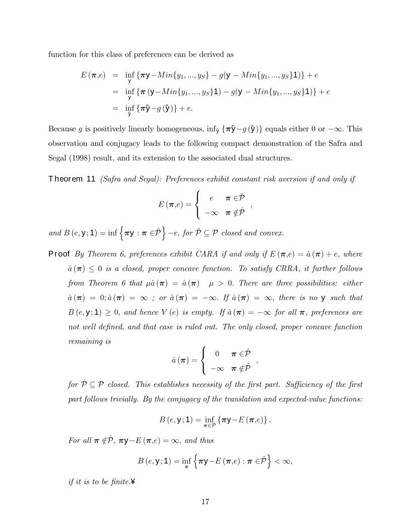
function for this class of preferences can be derived as

E (π,e) = infyπy−Miny1, ..., yS− g(y −Miny1, ..., yS1)+ e

= infyπ (y−Miny1, ..., yS1)− g(y −Miny1, ..., yS1)+ e

= infyπy−g (y)+ e.

Because g is positively linearly homogeneous, infy πy−g (y) equals either 0 or −∞. Thisobservation and conjugacy leads to the following compact demonstration of the Safra and

Segal (1998) result, and its extension to the associated dual structures.

Theorem 11 (Safra and Segal): Preferences exhibit constant risk aversion if and only if

E (π,e) =

e π ∈ P−∞ π /∈ P

,

and B (e,y;1) = infnπy : π ∈ P

o−e, for P ⊆ P closed and convex.

Proof By Theorem 6, preferences exhibit CARA if and only if E (π,e) = a (π) + e, where

a (π) ≤ 0 is a closed, proper concave function. To satisfy CRRA, it further follows

from Theorem 6 that µa (π) = a (π) µ > 0. There are three possibilities: either

a (π) = 0; a (π) = ∞ ; or a (π) = −∞. If a (π) = ∞, there is no y such that

B (e,y; 1) ≥ 0, and hence V (e) is empty. If a (π) = −∞ for all π, preferences are

not well deÞned, and that case is ruled out. The only closed, proper concave function

remaining is

a (π) =

0 π ∈ P−∞ π /∈ P

,

for P ⊆ P closed. This establishes necessity of the Þrst part. Sufficiency of the Þrst

part follows trivially. By the conjugacy of the translation and expected-value functions:

B (e,y;1) = infπ∈P

πy−E (π,e) .

For all π /∈ P, πy−E (π,e) =∞, and thus

B (e,y; 1) = infπ

nπy−E (π,e) : π ∈ P

o<∞,

if it is to be Þnite.¥

17

Besides exhaustively characterizing the class of constant risk averse preferences, Theorem

11 , when combined with the interpretation of the expected-value function as an expenditure

function in the presence of complete contingent claims, has an interesting consequence.

Corollary 12 Preferences exhibit constant risk aversion if and only if either ∂E (π, e) = e1

or ∂E (π, e) is undeÞned.

This corollary generalizes Yaaris (1987) observation that preferences in his dual model

display plunging behavior. That is, either the individual will reject a given risk entirely

and adopt a non-stochastic portfolio, or he will accept an amount of the risk that is either

unbounded or Þxed by the constraints of the choice problem. Corollary 12 establishes the

more general result that plunging behavior characterizes the entire class of quasi-concave,

constant risk averse preferences.

5 An Application to Convex Choice Sets

Following Peleg and Yaari (1975), we consider an individual faced with a closed, bounded,

convex choice set Y ⊆ <S. Such choice problems may arise, for example, from the standard

portfolio choice problem, the production decisions of a Þrm under uncertainty, or as an

investment allocation problem with nonlinear but appropriately convex tax structures. We

endow Y with the following properties 0 ∈Y, Y ∩<S++ 6= ∅.The decisionmakers choice problem is maxy e (y) : y ∈Y . Upon deÞning

R (π,Y ) = max πy : y ∈Y ,

and by restricting attention to the region where E is Þnite (see below for more on this

assumption), an equivalent dual formulation of the individuals choice problem is

maxπ,e

e : E (π,e) ≤ R (π,Y ) .

R (π,Y ) is the revenue function dual to Y that is associated with the state-claim prices π.

Observe that

R (π,Y + δu) = R (π,Y ) + δπu,

R (π,µY ) = µR (π,Y ) , µ > 0.

18

The optimization problem applies both when predetermined state-claim prices exist, as

they would, for example, in the presence of complete markets, or in the absence of any

predetermined state-claim prices. In the former case, optimization is over e, and equilibrium

e is determined by E (π,e) = R (π,Y ) . In a complete market, the decisionmaker maximizes

income given the state-claim prices, and then uses this income to purchase the bundle of

state-claims which maximize his preferences. This is analogous to equilibrium determination

for a small-open economy with a representative consumer.4

In the latter case, which is analogous to autarkic price determination in general equilib-

rium with a representative consumer, state-claim prices are chosen so that the individuals

internal market clears. Here it is convenient to recall E0s interpretation as a cost function.

Picking state-claim prices is thus equivalent to picking state-claim demands for E (π,e) and

state-claim supplies for R. Hence, the market clearing conditions require that there exist a

y ∈∂E (π,e) such thaty ∈ ∂R (π,Y ) ,

where the notation ∂R denotes the subdifferential of R in π. By Walras Law and the

basic properties of cost and revenue functions, one of the S market clearing conditions is

redundant (alternatively E (π,e) = R (π,Y ) is redundant in the presence of the S market

clearing conditions).

DeÞne the maximal nonstochastic income consistent with Y as

yY = max c : c1 ∈Y .

Dual to yY 1 is a set of risk-neutral probabilities, PY , which correspond to the supportinghyperplanes of Y at yY 1,

PY = ©π :yY 1 ∈∂R (π,Y )ª .R¡πY , Y

¢= yY ,πY ∈ PY . Besides offering the highest sure income that the decisionmaker

can realize from Y, because yY is always feasible, R¡πY , Y

¢= yY also places a lower bound

on equilibrium e and E (π,e).

Theorem 13 For any π consistent with the decisionmakers choice equilibrium, πY¹eπ ¹ π0,πY∈PY ,

where π0 are the maximally risk-neutral probabilities.4In this context, E (π,e)−R (π,Y ) is exactly analogous to a trade expenditure function

19

Proof Because R¡πY , Y

¢is feasible, E (π,e) ≥ yY = R ¡πY , Y ¢ , πY ∈ PY . By the deÞn-

ition of equilibrium, y ∈ ∂E (π,e) ∈ Y, and hence R ¡πY , Y ¢ ≥ πY y for any such y.

But it is also true that y ∈V (e) , whence πY y ≥E ¡πY , e¢ .¥In interpreting Theorem 13, one might think of πY as the set of minimally risky risk-

neutral probabilities determined by the structure of Y. They are the probabilities that would

lead a risk-neutral decisionmaker facing Y to choose the non-stochastic outcome. Theorem

13 is the preference analogue of the famous Peleg and Yaari (1975) result characterizing the

set of risk aversely efficient points over a general convex choice set. It implies that deci-

sionmakers choose state-contingent income allocations so that their equilibrium risk-neutral

probabilities are ranked between the minimally risky probabilities PY and the maximallyrisky π0. This means that their optimal state-contingent income vector must fall between

the nonstochastic portfolio, e1, and the portfolio that would be picked if the decisionmaker

were forced to make trades at πY ∈ PY . Figure 2 illustrates. Hence, just as the PelegYaarinotion of risk-averse efficiency constrains optimal choices of risk averters to lie in a particular

subset of a convex choice set, Theorem 13 restricts choice associated with Y to lie within

the subset of V (e) determined by these supporting hyperplanes.

Theorem 13 is true for general monotonic preferences and does not require convexity of

V (e) . It is a basic consequence of choice over convex sets. Among other things, the result

implies that individuals create perfect insurance in the face of such a convex choice problem

if and only if yY 1 ∈ ∂E ¡πY , yY ¢ for some πY ∈ PY , or, in other words, if and only if thechoice set permits them to create fair insurance at their maximally risk-neutral probabilities.

Now consider the class of preferences for which there exists a unique probability measure,

that is, for which π (1) is a singleton. Suppose that, for some initial choice set Y, equilibrium

is characterized by π 6= π (1) , so that the optimal y is not equal to e1. Then because

translating Y in the direction of 1 or radially expanding or shrinking Y has no effect on PY ,we conclude:

Theorem 14 If for some initial choice set, Y, equilibrium π 6= π (1) , then translating Y inthe direction of 1 or radially expanding or shrinking Y can only lead the decisionmaker to

adopt the nonstochastic portfolio if PY is not a singleton.

20

Thus, such shifts in Y can lead to the decisionmaker fully insuring only if Y exhibits a

kink at yY 1. A special case of this theorem is the well-known result that decisionmakers with

unique subjective probabilities will never fully insure if PY is a singleton but provides whatthe decisionmaker views as unfair odds. It is the choice set analogue of the result, derived by

Segal and Spivak (1991), that decisionmakers with Þrst-order risk aversion may fully insure

at unfair odds. Those results can be derived by an analogous argument, which is left to the

reader.

5.1 Comparative Statics for Linear Risk Tolerance and Constant

Risk Aversion

In the cases where preferences exhibit CARA and CRRA, the decisionmakers choice prob-

lem is particularly transparent. In the former, Theorem 6 implies that the decisionmaker

equilibrium is characterized by

eA (Y ) = maxe, π

e : e ≤ R (π,Y )− a ( π)= max

πR (π,Y )− a (π) ,

and in the latter by

eR (Y ) = maxπ

½R (π,Y )

r (π)

¾.

Because

R (π,Y + δ1) = R (π,Y ) + δ,

R (π,µY ) = µR (π,Y ) , µ > 0

one obtains the well-known results that a sure increase of wealth of δ dollars increases a

CARA individuals equilibrium e by δ, while a radial increase or decrease in wealth leads to

a proportionate change in the individuals equilibrium certainty equivalent. Similarly, for

the class of preferences translation homothetic in the direction of u,

eT (y) = max

½R (π,Y )− E0 (π)

πu

¾,

whence:

21

Theorem 15 If preferences are translation homothetic in the direction of u, replacing Y by

Y +δu with δ > 0 raises the equilibrium certainty equivalent by δ with no effect on equilibrium

π.

For the case of LRT, the equilibrium e is deÞned by

eL (Y ) = maxπ

½R (π,Y )−E0 (π)

E1 (π)

¾.

Denote the optimal choice of π by π and note that, since E1 (π) ≤ 1,

eL (Y + δ1) = maxπ

½R (π,Y ) + δ − E0 (π)

E1 (π)

¾≥ R (π,Y ) + δ −E0 (π)

E1 (π)

≥ eL (Y ) + δ,

which is to be expected in light of Theorem 10.

Now consider the archetypal comparative static changes: the replacement of the choice

set Y by tY for some t > 1 and the replacement of Y by Y + δ1 for some δ > 0. The Þrst

arises, for example, in the case of the Þrm under uncertainty facing a proportional increase

in all input and output prices. The second arises in the wealth allocation problem from an

exogenous, non-taxable increase in income.

Theorem 16 Suppose preferences exhibit LRT and are risk-averse with respect to some π0.

Replacement of Y by Y + δ1 for δ > 0 cannot lead to the choice of a less risky π, and

replacement of Y by tY for t > 1 cannot lead to the choice of a more risky π.

Proof The proof is for the replacement of Y by Y + δ1. Let π denote the originally optimal

choice of π and πδ the optimal choice for Y + δ1.

eL (Y + δ1) =R¡πδ,Y

¢+ δ − E0 ¡πδ¢E1 (πδ)

.

≥ R (π,Y ) + δ − E0 (π)E1 (π)

Now sinceR (π,Y )− E0 (π)

E1 (π)≥ R

¡πδ,Y

¢− E0 ¡πδ¢E1 (πδ)

22

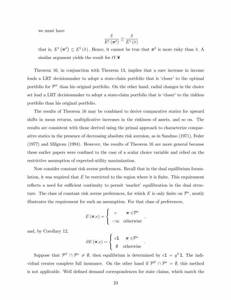
we must haveδ

E1 (πδ)≥ δ

E1 (π)

that is, E1¡πδ¢ ≤ E1 (π) . Hence, it cannot be true that πδ is more risky than π. A

similar argument yields the result for tY.¥

Theorem 16, in conjunction with Theorem 13, implies that a sure increase in income

leads a LRT decisionmaker to adopt a state-claim portfolio that is closer to the optimal

portfolio for PY than his original portfolio. On the other hand, radial changes in the choiceset lead a LRT decisionmaker to adopt a state-claim portfolio that is closer to the riskless

portfolio than his original portfolio.

The results of Theorem 16 may be combined to derive comparative statics for upward

shifts in mean returns, multiplicative increases in the riskiness of assets, and so on. The

results are consistent with those derived using the primal approach to characterize compar-

ative statics in the presence of decreasing absolute risk aversion, as in Sandmo (1971), Feder

(1977) and Milgrom (1994). However, the results of Theorem 16 are more general because

these earlier papers were conÞned to the case of a scalar choice variable and relied on the

restrictive assumption of expected-utility maximization.

Now consider constant risk averse preferences. Recall that in the dual equilibrium formu-

lation, it was required that E be restricted to the region where it is Þnite. This requirement

reßects a need for sufficient continuity to permit market equilibration in the dual struc-

ture. The class of constant risk averse preferences, for which E is only Þnite on P∗, neatlyillustrates the requirement for such an assumption. For that class of preferences,

E (π,e) =

e π ∈P∗

−∞ otherwise,

and, by Corollary 12,

∂E (π,e) =

e1 π ∈P∗∅ otherwise

.

Suppose that PY ∩ P∗ 6= ∅, then equilibrium is determined by e1 = yY 1. The indi-

vidual creates complete full insurance. On the other hand if PY ∩ P∗ = ∅, this methodis not applicable. Well deÞned demand correspondences for state claims, which match the

23

supplies generated from R (π,Y ) , do not exist. Instead, equilibrium, is determined by the

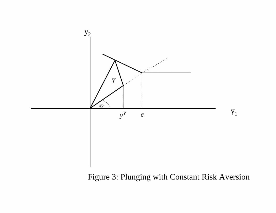
decisionmaker plunging to the bounds of the choice set as

maxyinf πy : π ∈P∗ : y ∈Y = inf R (π,Y ) : π ∈P∗ ,

The choice problem reduces to Þnding the least favorable R (π,Y ) consistent with π ∈P∗.Figure 3 illustrates plunging behavior for the standard portfolio problem, with one safe

asset, one risky asset, and no short selling. This latter characterization of equilibrium be-

havior always holds under constant risk aversion. We say that plunging exists when the dual

equilibration process approach outlined above cannot be used in place of this latter charac-

terization. By observing that PY is invariant to either radial changes in Y or translations

of Y in the direction of the sure thing, we can characterize comparative statics compactly

under constant risk aversion by:

Theorem 17 If the decisionmaker has constant risk averse preferences, her equilibrium cer-

tainty equivalent is given by inf R (π,Y ) : π ∈P∗ . Replacing Y by Y + δ1 shiÞts the equi-librium certainty equivalent by δ, and replacing Y by tY for t > 0 rescales the equilbrium

certainty equivalent by t. If the decisionmaker plunges before Y is replaced by Y + δ1 or by

tY, she will plunge after the replacement. If she does not plunge before these replacements,

she will not plunge after these replacements.

6 Concluding comments

Dual approaches have proved their value in many areas of economic analysis. Until recently,

however, the analysis of choice under uncertainty has made little use of duality concepts.

Instead reliance has been placed almost exclusively on primal methods, and, in particular, on

the expected-utility model. Perhaps the best explanation of the endurance of the expected-

utility model, in spite of its well-known weaknesses, is its ability to yield predictions about

economic behavior. Much of the predictive bite of the expected utility model comes from

what many regard as its Achilles heel, the independence axiom and its consequent additive

separability.

24

Additively separable preferences were discarded as a reasonable representation of prefer-

ences in standard consumer theory long ago . Instead, reliance is usually placed on direct

assumptions about the nature of the decisionmakers preference map. In particular, the

notions of homotheticity and quasi-homotheticity have proven very useful in both empirical

and theoretical analyses. These restrictions have percolated into expected-utility theory,

albeit in disguised form, as the notions of CARA, CRRA, and LRT. This paper has taken

advantage of this equivalence and the dual formulation to show how behavior can be fully

characterized without imposing additive separability, and that a dual formulation of choice

under uncertainty is both straightforward and analytically productive.

25

Reference List

Blackorby, C., and D. Donaldson. A Theoretical Treatment of Indices of Absolute

Inequality. International Economic Review 21, no. 1 (February1980): 10736.

Blackorby, C., R. Boyce, and R. R. Russell. Estimation of Demand Systems Generated

by the Gorman Polar Form: A Generalization of the SBranch Utility Tree. Econometrica

46 (1978): 34564.

Brennan, M. J., and A. Kraus. The Geometry of Separation and Myopia. Journal of

Financial and Quantitative Analysis 11 (1976): 17193.

Cass, D., and J. E. Stiglitz. The Structure of Investor Preferences and Asset Returns,

and Separability in Portfolio Allocation: A Contribution to the Pure Theory of Mutual

Funds. Journal of Economic Theory 2 (1970): 12260.

Chambers, R. G. Consumers Surplus As an Exact and Superlative Cardinal Welfare

Measure. International Economic Review 42 (2001): 10520.

Chambers, R. G., and J. Quiggin. Uncertainty, Production, Choice, and Agency: The

StateContingent Approach. New York: Cambridge University Press, 2000.

Chambers, R. G., and R. Färe. Translation Homotheticity. Economic Theory 11

(1998): 62941.

Chambers, Robert G., Y. Chung, and R. Fare. BeneÞt and Distance Functions. Journal

of Economic Theory 70 (1996): 40719.

Dickinson, J. G. Parallel Preference Structures in Labour Supply and Commodity De-

mand: An Adaptation of the Gorman Polar Form. Econometrica 48 (November1980):

171125.

Epstein, L. G., and S. E. Zin. FirstOrder Risk Aversion and the Equity Premium

Puzzle. Journal of Monetary Economics 26 (1990): 387407.

Feder, G. The Impact of Uncertainty on a Class of Objective Functions. Journal of

Economic Theory 16 (1977): 50412.

Gorman, W. M. Community Preference Fields. Econometrica 21 (1953): 6380.

Karni, E. Decision Making Under Uncertainty: The Case of StateDependent Prefer-

ences. Cambridge: Harvard University Press, 1985.

26

Lewbel, A. The Rank of Demand Systems: Theory and Nonparametric Estimation.

Econometrica 59 (May1991): 71130.

Lewbel, A., and W. Perraudin. A Theorem on Portfolio Selection With General Pref-

erences. Journal of Economic Theory 65 (1995): 62426.

Luenberger, D. G. BeneÞt Functions and Duality. Journal of Mathematical Economics

21 (1992): 46181.

Machina, M. J. Payoff Kinks in Preferences Over Lotteries. Journal of Risk and Un-

certainty 23 (2001): 20760.

Milgrom, Paul. Comparing Optima: Do Simplifying Assumptions Affect Conclusions.

Journal of Political Economy, no. 3 (1994): 60715.

Milne, F. Consumer Preferences, Linear Demand Functions, and Aggregation in Com-

petitive Asset Markets. Review of Economic Studies 46 (1979): 40717.

Nau, R. A Generalization of PrattArrow Measure to NonExpected Utility Preferences

and Inseparable Probability and Utility. Working Paper, Fuqua School of Business, Duke

University, 2001.

Peleg, B., and M. Yaari. A Price Characterisation of Efficient Random Variables.

Econometrica 43 (1975): 28392.

Quiggin, J., and R. G. Chambers. Risk Premiums and BeneÞt Measures for Generalized

Expected Utility Theories. Journal of Risk and Uncertainty 17 (1998): 12138.

Rockafellar, R. T. Convex Analysis. Princeton: Princeton University Press, 1970.

Safra, Zvi, and Uzi Segal. Constant Risk Aversion. Journal of Economic Theory 83,

no. 1 (1998): 1942.

Sandmo, A. On the Theory of the Competitive Firm Under Price Uncertainty. Amer-

ican Economic Review 61 (1971): 6573.

Segal, U., and A. Spivak. FirstOrder Versus SecondOrder RiskAversion. Journal

of Economic Theory 51, no. 1 (1990): 11125.

Yaari, M. Convexity in the Theory of Choice Under Risk. Quarterly Journal of Eco-

nomics 79 (May1965): 27890.

. The Dual Theory of Choice Under Risk. Econometrica 55 (1987): 95115.

. Some Remarks on Measures of Risk Aversion and on Their Uses. Journal of Economic

27

Theory 1 (1969): 31529.

28

y2

y145o

V(e)

eE(π, e)

Figure 1: Certainty Equivalent and E(π, e)

y2

y145o

V(e)

e

Figure 2: Range of Equilibrium Probabilities

yY

PY

π0

Y

y2

y145o

e

Figure 3: Plunging with Constant Risk Aversion

yY

Y