dual-ekf-based real-time celestial navigation for …...dual-ekf-based real-time celestial...

Hindawi Publishing CorporationMathematical Problems in EngineeringVolume 2012, Article ID 578719, 16 pagesdoi:10.1155/2012/578719

Research ArticleDual-EKF-Based Real-Time Celestial Navigationfor Lunar Rover

Li Xie,1, 2 Peng Yang,1, 2 Thomas Yang,3 and Ming Li4

1 Department of Information Science and Electronic Engineering, Zhejiang University,Hangzhou 310027, China

2 Zhejiang Provincial Key Laboratory of Information Network Technology, Hangzhou 310027, China3 The Department of Electrical, Computer, Software, and Systems Engineering, Embry-RiddleAeronautical University, Daytona Beach, FL 32114, USA

4 School of Information Science and Technology, East China Normal University,Shanghai 200241, China

Correspondence should be addressed to Li Xie, [email protected]

Received 27 December 2011; Accepted 14 February 2012

Academic Editor: Carlo Cattani

Copyright q 2012 Li Xie et al. This is an open access article distributed under the CreativeCommons Attribution License, which permits unrestricted use, distribution, and reproduction inany medium, provided the original work is properly cited.

A key requirement of lunar rover autonomous navigation is to acquire state information accuratelyin real-time during its motion and set up a gradual parameter-based nonlinear kinematics modelfor the rover. In this paper, we propose a dual-extended-Kalman-filter- (dual-EKF-) based real-time celestial navigation (RCN) method. The proposed method considers the rover position andvelocity on the lunar surface as the system parameters and establishes a constant velocity (CV)model. In addition, the attitude quaternion is considered as the system state, and the quaterniondifferential equation is established as the state equation, which incorporates the output of angularrate gyroscope. Therefore, the measurement equation can be established with sun direction vectorfrom the sun sensor and speed observation from the speedometer. The gyro continuous outputensures the algorithm real-time operation. Finally, we use the dual-EKFmethod to solve the systemequations. Simulation results show that the proposed method can acquire the rover positionand heading information in real time and greatly improve the navigation accuracy. Our methodovercomes the disadvantage of the cumulative error in inertial navigation.

1. Introduction

In order to conduct scientific exploration on the lunar surface, lunar rover must have theability to execute tasks in unstructured environment. Its navigation system must have ahigh degree of autonomy and the capabilities of high-accuracy real-time positioning andorientation. On lunar surface, some commonly used navigation methods on the earth are not

2 Mathematical Problems in Engineering

applicable. There is no GPS system on the moon. If we use radio navigation, the rover controlmay fail because of the two-way communication delay. The moon rotation is very slow, so wecannot use north seeking gyro. Also, lunar magnetic field is very weak, so magnetic sensor-based methods are ineffective.

Lunar rover navigation techniques mainly include absolute positioning and relativepositioning. For absolute positioning, such as autonomous celestial navigation [1], positionand heading errors are bounded and do not accumulate over time, and the output is discrete.The initial positioning is generally absolute positioning, and its accuracy directly affectsrelative positioning accuracy. Relative positioning, such as inertial navigation, achieves highaccuracy of position and heading in short time, but the errors accumulate over time (whichmay lead to divergence), and the output is continuous. The current trend for lunar rovernavigation is integrated navigation, which combines the advantages of celestial navigationand inertial navigation.

The earliest researchers [2–4] carried out celestial navigation by the altitude differencemethod through observing the sun, earth, and fixed stars. Kuroda et al. [5] utilized celestialnavigation and dead-reckoning-based integrated navigation method to obtain lunar rover’sabsolute position and heading, which is achieved by observing the altitude and azimuth ofthe sun and the earth. However, on the moon, the time period during which the sun andthe earth appear simultaneously is very short. Therefore, the application of this method islimited. Altitude difference method is very sensitive to measurement noise, and positioningaccuracy [6] is low. Vision-based navigation is often used in robotics (Chen 2012, see [7, 8]),but it has difficulty in determining the absolute location and attitude.

Recent researchers use vector-observations-based quaternion estimation (QUEST) toget the rover heading angle [9–12]. Ashitey proposed an absolute heading detection methodfor the field integrated, design and operation (FIDO) rover [9]. When stopped, it uses sunsensor and accelerometer to sense the sun orientation and the local gravity orientation, supplyabsolute heading for rover with QUEST, and correct the gyroscope cumulative error. Alidescribed that the US Mars rovers (the “Hope” and the “Spirit”) utilized this method to self-correct the heading information [10]. Some recent technologies used in robotics can be foundin the works of Chen et al. [13]. Methods in Chinese literature are similar to the methodby Ashitey and they also calculate the heading through QUEST [11, 12]. Thein analyzedthe relationship between lunar rover positioning accuracy and astronomical instrumentmeasurement noise [14]. If we want to limit the position error within 50m, measurementnoise should be less than 5.93 arcsec.

The above celestial navigation methods (except [5]) do not combine celestialpositioning with orientation and cannot get the absolute heading and location informationin real time. Ning established a position and attitude determination method based oncelestial observations [15], but its reference frame is moon fixed coordinate system ratherthan local level coordinate system, and it does not consider the impact of the position andspeed changes on the gyro angular rate output. Ning proposed a lunar rover kinematicsmodel-based augmented unscented particle filter (ASUPF) as a new autonomous celestialnavigation method for dealing with systematic errors andmeasurement noise [16]. However,the altitude angle measurements in this method are based on the local level provided bythe inertial measurement unit (IMU), assuming the rover is keeping static or in constantmotion. When the rover is moving, it needs the support of attitude update algorithm ininertial navigation, because the gyro accumulates error and the local level precision is low. Peiproposed a strapdown inertial navigation and celestial-navigation-based integrated methodfor lunar rovers [17].

Mathematical Problems in Engineering 3

Since lunar rover position change on the lunar surface is very slow, in order to reducethe dimension of the system, we can set position as a gradual system parameter to estimatethe rover state, that is, heading and attitude. To correct the position of the lunar rover, thevelocity observation is introduced.Meanwhile, in order to obtain real-time navigation output,the output of the gyro is needed in integrated navigation. In this paper, a method of real-timecelestial navigation is proposed, in which positioning and orientation are simultaneous. Also,the error bounded sun sensor output and high accuracy rate gyro output are fused, whichensures the navigation output to be both real-time and of higher accuracy when the roveris moving. Because there is no accelerometer in the system, the impact of the accelerometererror and gravity anomaly on navigation is avoided.

The organization of the paper is as follows. Section 1 describes the principles ofcelestial navigation and attitude quaternion kinematics. Section 2 describes the dual EKF-based real-time celestial navigation method. Section 3 presents the results of computersimulations and compares the accuracy of the results obtained with and without velocityobservation. Section 4 presents conclusions and discussions.

2. Celestial Navigation Principle and Attitude Kinematics

2.1. Principle of Celestial Navigation

Set the selenocenter celestial coordinate system as the inertial coordinate system (i), the moonfixed coordinate system asm, geographic coordinate system (NED) as n, the lunar rover bodycoordinate system as b, the local level coordinate system as l, and the sun sensor coordinatesystem as c. After installation, the sensor coordinate systems b and c coincide with each other.

Celestial navigation system can detect the rover geographical position and headingprovided that the local gravity datum (level posture) is known. The outputs are lunar roverposition (latitude and longitude) on the moon and the attitude, including the heading, pitch,and roll. State vector of the system x = [λ, L,An] is used to describe the lunar rover positionand heading information, in which (λ, L) is the lunar rover longitude and astronomicallatitude and An is just heading relative to North Pole of the moon.

In Figure 1, the moon fixed coordinate system, after rotating λ (east longitude ispositive) around the Z axis, becomes coordinate system O − x1y1z1. After further rotatingby −L − π/2 (north latitude is positive) around the Oy1 axis, the navigation coordinate w isobtained. The attitude matrix about the latitude and longitude is as follows [18]:

nm� = �y

(−L − π

2

)�z(λ). (2.1)

The attitude matrix about the navigation coordinate system and the lunar body coordinatesystem is:

bn� = �x

(ϕ)�y

(ψ)�z(θ). (2.2)

Here, θ is the heading, ψ is the pitch angle, and ϕ is the roll. To prevent the risk of rollover,lunar rover pitch and roll should between ±45◦. The attitude matrix about the moon fixedcoordinate system and the local level coordinate system is A = l

m� (called target matrix


Moon-fixedframe

The moon

The sunNorth-Earth-down

frame

Zm

Om

Ym

Xn

Yn

OnZn

Xm

L

λ

Figure 1: Moon-fixed (m) and navigation (n) coordinate system.

here). Substituting �z(θ), �y(−L − π/2),�z(λ) into the above formula, we get the followingequation:

lm� = �z(θ) �y

(−L − π

2

)�z(λ). (2.3)

2.2. Quaternion Attitude Kinematics

Attitude can be expressed in several mathematical parameters: quaternion, attitude matrix,Euler angles, Rodrigues parameters, and so on. The attitude matrix contains a total of nineparameters, but because it is orthogonal matrix, only three components are independent. Oneof the most useful parameters is the attitude quaternion, which is a four-dimensional vector,defined as q = [ρT q4]

T , where ρ = [q1 q2 q3]T = e sin(ϑ/2) and q4 = cos(ϑ/2). Here, e is the

rotation axis and ϑ is the rotation angle. When using a four-dimensional vector to describethe three-dimensional rotation, the four parameters of quaternion are not independent, andthey are subject to the constraint qTq = 1. The relationship between the attitude matrix andthe quaternion from the inertial coordinate system i to the body coordinate system b is

biA(q) = ΞT (q)Ψ(q), (2.4)

where

Ξ(q) ≡[q4I3×3 + [ρ×]

−ρT], Ψ(q) ≡

[q4I3×3 − [ρ×]

−ρT]· Ξ(q) ≡

[q4I3×3 + [ρ×]

−ρT],

Ψ(q) ≡[q4I3×3 − [ρ×]

−ρT].

(2.5)


Here [ρ×] is the cross-product matrix, defined as [ρ×] =[ 0 −q3 q2

q3 0 −q1−q2 q1 0

]. One advantage of using

quaternion is that the attitude matrix is quadratic equation of the parameter and thus doesnot include any transcendental function. For small angles, the vector part of the quaternionis approximately half of the rotation angle, and therefore ρ ≈ α/2, q4 ≈ 1, where the 3-dimensional vector α includes roll, pitch, and heading. Therefore, the attitude matrix can beapproximated as b

iA ≈ I3×3 − [α×], which is effective in the first-order approximation.The attitude kinematics equation is

bi A = −

[ωbib×

]biA . (2.6)

Here, ωbib is the angular velocity of the b frame relative to i frame expressed in b coordinates.

The quaternion differential equation is

q =12Ξ(q)ωb

ib =12Ω(ωbib

)q, (2.7)

where

Ω(ωbib

)≡

⎡⎢⎣−[ωbib×

]ωbib

−(ωbib

)T0

⎤⎥⎦. (2.8)

The main advantage of using the quaternion is that the kinematics equation is linearand there is no singularity. Another advantage is that continuous rotation of coordinateframes can be expressed as the quaternion multiplication. Suppose a continuous rotation canbe expressed as

A(q′)A(q) = A

(q′ ⊗ q

). (2.9)

The composition of the quaternion is bilinear, with

q′ ⊗ q =[Ψ(q′) q′]q = [Ξ(q) q]q′, (2.10)

and the inverse quaternion is defined by q−1 =[ −ρq4

]. Note that q ⊗ q−1 = [ 0 0 0 1 ]T is the

identity quaternion.

3. Dual-EKF-Based RCPO Method

Assume the state vector of the navigation system is xs, the system parameter vector is xp, andthe observation vector is yk. According to the problem, a continuous-discrete nonlinear statespace model can be derived:

xs(t) = f{t, xs(t),u(t), xp(t)

}+w(t),

yk = hk(xs,k, xp,k

)+ vk,

(3.1)


where f(·), h(·) are implicit vector functions, w(t) is the continuous process noise, and vkis the discrete measurement noise. In the state vector xs = [qT , βT ]T , q is the heading andattitude quaternion in the navigation frame (w) for the lunar rover and β is the constant biasfor gyro. In parameter vector xp = [pT , vT ]T , p = [L λ]T is the rover position, which is thelatitude and longitude; V = [vL vλ]

T is the north speed and east speed on the lunar surface.

3.1. System Parameter and State Equations

The lunar rover position and velocity equations constitute the system parameter equations:

xp = Fpxp +wp (3.2)

with the parameter vector xp = [pT VT ]T , the state transition matrix Fp =[ 0 0 1 00 0 0 10 0 0 00 0 0 0

], the

parameters process noise wp =[ 0

0wLwλ

], and the noise covariance Qp = diag[0 0 σ2

L σ2λ].

The lunar rover attitude constitutes the system state equations, and the quaterniondifferential equation is expressed by

q2 =12Ω(ωb

nb

)q2. (3.3)

Here,ωbnb is the angular velocity of the b frame relative to n frame expressed in b coordinates.

The gyro measurement model is

ωbib = ω

bib + β + ηv,

β = ηu.(3.4)

Here, ωbib is the angular velocity of the b frame relative to i frame expressed in b coordinates.

β is the constant bias of the gyro, ηv and ηu are zero mean Gaussian white noise processs, andtheir spectral density functions are σ2

vI3×3 and σ2uI3×3, respectively.

Because the selenocenter celestial coordinate system is the inertial coordinate systemhere, so

ωbnb = ω

bib − b

nA(q2)ωnin. (3.5)

Also, ωnin is the angular velocity of the n frame relative to i frame expressed in n coordinates

ωnin = ωim

⎡⎣

cosL0

− sinL

⎤⎦ +

⎡⎢⎢⎢⎢⎢⎢⎢⎣

VER

−VNR

−VE tanLR

⎤⎥⎥⎥⎥⎥⎥⎥⎦, VE = vλR cosL, VN = vLR. (3.6)


In (3.6), ωim is the angular velocity of the m frame relative to i frame, and the secondexpression on the right side is the angular velocity of the n frame relative to m frame. Theangular velocity of them frame relative to i frame ωim is

ωim = ωgz + mi Aωzz . (3.7)

In (3.7), ωgz is the revolution angular velocity of the moon around the earth, ωzz is the moonspin velocity, and m

i A is the attitude matrix from the inertial reference frame i to the moonfixed framem, which can be calculated after querying ephemeris [18].

3.2. Celestial and Speed Observation Equations

The measurement principle of vector observation attitude sensor can be expressed as bi =A(q)ri + vi, i = 1, . . . , n. If n celestial bodies are observable simultaneously, we can get nvector pairs, so the measurement equation at time k is

bk =

⎡⎢⎢⎢⎣

A(q2)A(p1)r1A(q2)A(p1)r2

...A(q2)A(p1)rn

⎤⎥⎥⎥⎦

∣∣∣∣∣∣∣∣ tk+

⎡⎢⎢⎢⎣

v1v2...vn

⎤⎥⎥⎥⎦

∣∣∣∣∣∣∣∣ tk, (3.8)

where A(q2) = bnA, A(p1) = n

mA = �y(−L − π/2)�z(λ).

Set vk =

⎡⎣

v1v2...vn

⎤⎦∣∣∣∣ tk , its variance is R = diag[σ2

1I3×3, σ22I3×3, . . . , σ

2nI3×3], where diag[· · ·]

is the diagonal matrix. In this paper, n = 1, r = is, b = bs, where is is the sun unit vector ininertial frame and bs is the sun unit vector in the body frame.

The speed observation equation of the speedometer is

Vk = Vk + uk, (3.9)

where Vk is speed measurement at time k, uk is the measurement noise, and its covariancematrix is Ru = σ2

uI2×2.

3.3. Dual Continuous-Discrete EKF

Dual-EKF algorithm uses two mutual coupling extended Kalman filters working in paralleland a state estimator working between the system parameter time update process and themeasurement update process [19]. Dual-EKF can estimate the system state and parameteronline. Using the above model, a continuous-discrete extended Kalman filter can be derived(Chen 2012, [20]). The process equation about the system parameter is a continuous linearequation, which can be discretized directly. The process equations about the system state


are nonlinear equations, and the Jacobian matrix needs to be calculated. Finally, we get thediscrete linear state space model (without considering the control input uk):

xs,k+1 = f{xs,k, xp,k

}+wk,

yk = hk(xs,k, xp,k

)+ vk.

(3.10)

3.3.1. Linearization of State Process Equations

In order to maintain the quaternion normalization constraint, we use the multiplicative errorquaternion in the body frame to express the attitude error:

δq = q ⊗ q−1, (3.11)

where q−1 is the inverse of the quaternion estimate and δq ≡ [δρT δq4]T . If the error

quaternion δq is very small, we can use the small angle approximation. After a series ofderivation, the linear kinematic model of the attitude error [21] is obtained:

δα = −[ωbnb×

]δα + δωb

ib −A(q2)δωnin, δq4 = 0, (3.12)

where δωbib= ωb

ib− ωb

iband δωn

in = ωnin − ωn

in = 0. Also, δωbib= −(Δβ + ηv) is available by the

above gyro model, in which Δβ ≡ β − β. So the above formula becomes

δα = −[ωbnb×

]δα − (

Δβ + ηv). (3.13)

The remaining error equation can be obtained by similar methods. The state vector,the state error vector, and the process noise vector and covariance in this EKF are defined as

xs ≡[qβ

], Δxs ≡

[δαΔβ

], ws ≡

[ηvηu

], Qs =

[σ2vI3×3 03×303×3 σ2

uI3×3

]. (3.14)

The error dynamics of time update in the EKF is Δx = FΔx + Gw. Here, the statetransition matrix F and the noise coefficient matrix G are

F ≡[−[ωbnb×

]−I3×3

03×3 03×3

], G ≡

[−I3×3 03×303×3 I3×3

]S. (3.15)

3.3.2. Linearization of Measurement Equations

Next we determine the sensitive matrixHs(x−s ) of the system state observation equation. Thetrue value and the estimate of the celestial bodies vector in the body coordinate system are

b = A(q2)A(p−1

)r, b− = A

(q−2

)A(p−1

)r. (3.16)


According to (2.6),

A(q2) = A(δq2)A(q−2

)= (I3×3 − [δα2×])A

(q−2

). (3.17)

From (3.16), we have

Δb = b − b− =[A(q−2

)A(p−1

)r×]δα2. (3.18)

Note that Hsq = [A(q−2 )A(p−

1 )r×], so the sensitivity matrix for all measurements is

Hs

(x−s)=

⎡⎢⎢⎢⎣

Hsq1 03×3Hsq2 03×3

......

Hsqn 03×3

⎤⎥⎥⎥⎦

∣∣∣∣∣∣∣∣ tk. (3.19)

Next we determine the sensitive matrix Hp(x−p) of the system parameter observationequation.

The true value and the estimate of the celestial bodies vector in the body coordinatesystem are

b = A(q−2

)A(p)r, b− = A

(q−2

)A(p−)r. (3.20)

Function A(p) is expanded as a Taylor series, which is

A(p) ≈ A(p−) +

2∑j=1

A−j Δpj , (3.21)

where A−1 = ∂A/∂L|L− , A−

2 = ∂A/∂L|λ− .Finally, we have

Δb = b − b− =2∑j=1

A(q−2

)A−j rΔpj . (3.22)

Note that Hp =[A(q−

2 )A−1 r A(q−

2 )A−2 r

]. Combined with the speed observations, the

sensitivity matrix of all measurements is

Hp

(x−p)=

⎡⎢⎢⎢⎢⎢⎢⎣

Hp1 03×2Hp2 03×2...

...Hpn 03×202×2 I2×2

⎤⎥⎥⎥⎥⎥⎥⎦

∣∣∣∣∣∣∣∣∣∣∣ tk

. (3.23)


Table 1: Dual-EKF algorithm.

Initialization Parameter: xp(t0) = xp,0, Pp(t0) = Pp,0State: xs(t0) = xs,0, Ps(t0) = Ps,0

State measurement update

Ks,k = P−s,kHT

s,k[Hs,kP

−s,kHT

s,k+ R]−1

εk = bs,k − hk(x−s,k, x−

p,k)

Δx+s,k

= Ks,kεk

q+2,k = q−

2,k +12Ξ(q−

2,k)δα+2,k , normalization

β+k = β

−k + Δβ

+k

P+s,k

= [I −Ks,kHs,k]P−s,k

Parameter measurement update

Kp,k = P−p,kHT

p,k[Hp,kP

−p,kHT

p,k+ R′]−1

R′ = diag([R,Ru])x+p,k

= x−p,k

+Kp,k[εk ; (Vk − V−k)]

P+p,k

= [I −Kp,kHp,k]P−p,k+1

Parameter time updatex−p,k+1 = Φpx

+p,k

P−p,k+1 = ΦpP

+p,k

ΦTp +Qp

State time update

ωbnb

= (ωbib− β+

k) −A(q+

2,k)ωnin(x

−p,k+1)

˙q2 =12Ω(ωb

nb)q2

˙β = 0Ps = FsPs + PsFsT +GQsG

T

3.3.3. Dual-EKF Algorithm

Finally the proposed algorithm of dual-EKF is shown in Table 1.

4. Simulations and Discussions

4.1. Simulation Conditions

Specific simulation parameters are shown in Table 2.

4.2. Simulation of Moving Lunar Rover

In this paper, we carried out lunar rover simulation under various moving conditionsdescribed in Table 3, and navigation accuracy with and without the speed observation iscompared. The lunar rover movement includes rotational and translational movements,where the former can be sensed by the gyro angular velocity and the latter can be measuredby the speedometer line speed.

The simulation results of the lunar rover are shown in Figure 2, with the left diagramon each figure representing the simulation result without speed observation and the rightdiagram representing the simulation result with speed observation.

Figure 2 shows the position error and its 3σ boundary, and we see the latitude andlongitude errors in the left diagram diverge at last. After the uniform motion error expands,we mainly have the lunar rover speed changes, so the constant velocity (CV) model is no


0 200 400 600

0

50

100

−100

−50

Time (s)

Lat

itud

e(a

rcse

c)

(a)

0 200 400 600

0

50

100

−100

−50Lat

itud

e(a

rcse

c)

Time (s)

(b)

0 200 400 600

0

50

100

Time (s)

−100

−50Lon

gitu

de(a

rcse

c)

(c)

0 200 400 600

0

50

100

Lon

gitu

de(a

rcse

c)

Time (s)

−100

−50

(d)

Figure 2: Position error and 3σ boundary.

Table 2: Simulation parameters.

Beginning time 2011-01-01 00:00:00

Sampling interval Δt = 1 s

Initial origin λ(t0) = 0◦, L(t0) = 0◦

Initial velocity vL = −0.1m/(s · R), vλ = 0.1m/(s · R)Initial attitude q(t0) = [ 0 0 0 1 ]T

Gyro biases β(t0) = 0.1[ 1 1 1 ]T deg/hr

Initial covariance

Pp

0 = 0.052 deg2

PV0 = 0.12(m/s)2

Pα0 = 0.12 deg2

Pβ

0 = 0.22(deg/hr)2

Gyro noise (Qs)σgv =

√10 × 10−7 rad/s1/2

σgu =√10 × 10−10 rad/s3/2

CV model (Qp)σL = σL = 0.0001m/(s · R)(R: moon radius, the same below)

Sun sensor (R) 1′(3σs)

Velocity sensor (Ru) σu = 0.001m/(s · R)


0 200 400 600

0

0.2

0.4

−0.4

−0.2

Time (s)

Vel

ocit

y la

titu

de(m

/s)

(a)

Time (s)

Vel

ocit

y la

titu

de(m

/s)

0 200 400 600−0.04

−0.02

0

0.02

0.04

(b)

0 200 400 600

0

0.2

0.4

Vel

ocit

y lo

ngit

ude(m

/s)

−0.4

−0.2

Time (s)

(c)

0 200 400 600

0

0.02

0.04

Vel

ocit

y lo

ngit

ude(m

/s)

−0.04

−0.02

Time (s)

(d)

Figure 3: The speed error and 3σ boundary.

Table 3: Lunar rover motion.

Motion Time (s) Angular velocity( ◦/s)

Linear velocity(m/(s · R))

(1) Static 1∼100 0 0

(2) Rotation 101∼200 ωz = 1 0

(3) Uniform motion 201∼300 0 vL = 0.2vλ = −0.25

(4) Rotation and uniform motion 301∼500 ωz = 1 vL = 0.2vλ = −0.25

(5) Static again 501∼600 0 0

longer applicable. The navigation error in the right diagram is kept within the 3σ boundary,and it does not diverge. Because of the speedometer line speeds information, the absoluteposition of the rover can be adjusted in real time. The mean of the latitude error is 3.97

′′,

and the standard deviation is 0.83′′; the mean of longitude error is 1.07

′′, and the standard

deviation is 1.42′′. Converted into the line error according to the lunar radius, the error is

35.51m.


0 200 400 600

0

100

−100

Rol

l(ar

csec)

Time (s)

(a)

0 200 400 600

0

100

−100

Rol

l(ar

csec)

Time (s)

(b)

0 200 400 600

0

100

Pitc

h (a

rcse

c)

−100

Time (s)

(c)

0 200 400 600

0

100

Pitc

h (a

rcse

c)

Time (s)

−100

(d)

0 200 400 600

0

100

Yaw

(arc

sec)

−100

Time (s)

(e)

0 200 400 600

0

100

Yaw

(arc

sec)

Time (s)

−100

(f)

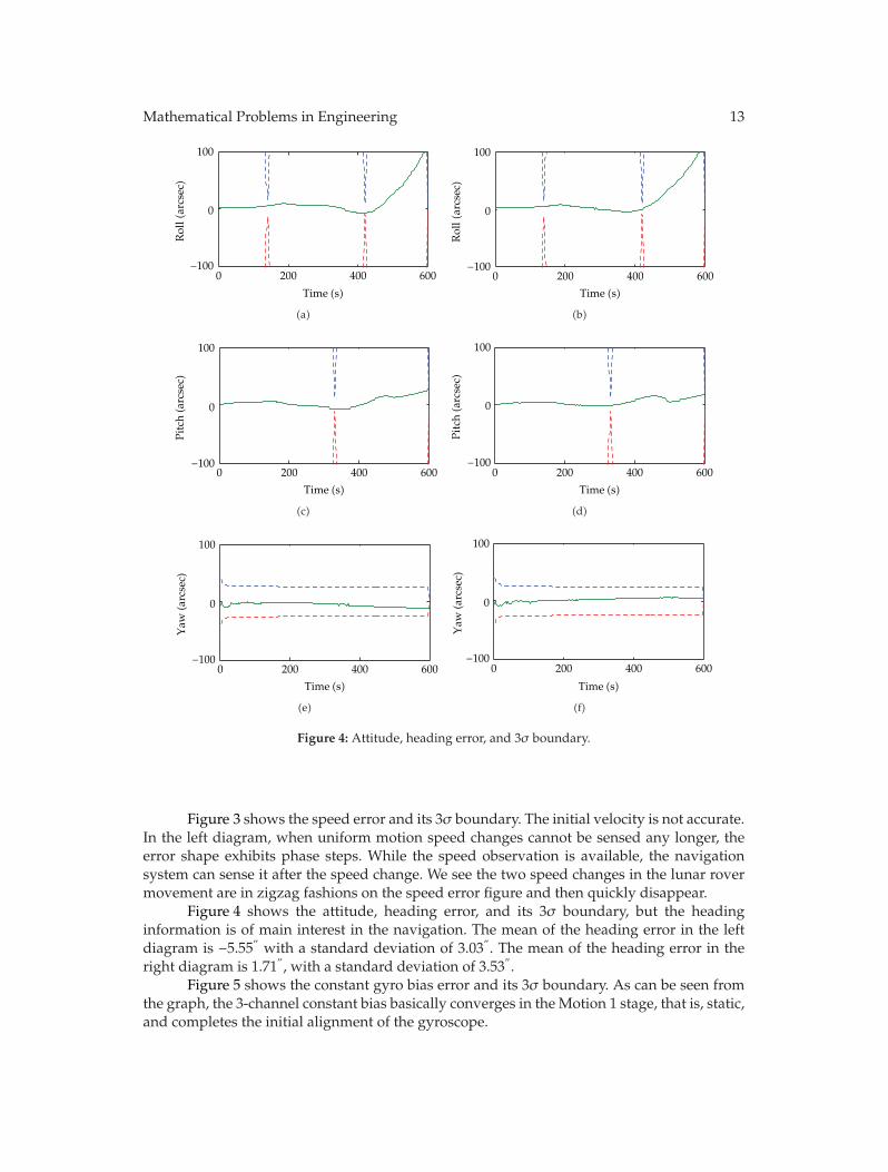
Figure 4: Attitude, heading error, and 3σ boundary.

Figure 3 shows the speed error and its 3σ boundary. The initial velocity is not accurate.In the left diagram, when uniform motion speed changes cannot be sensed any longer, theerror shape exhibits phase steps. While the speed observation is available, the navigationsystem can sense it after the speed change. We see the two speed changes in the lunar rovermovement are in zigzag fashions on the speed error figure and then quickly disappear.

Figure 4 shows the attitude, heading error, and its 3σ boundary, but the headinginformation is of main interest in the navigation. The mean of the heading error in the leftdiagram is −5.55” with a standard deviation of 3.03”. The mean of the heading error in theright diagram is 1.71”, with a standard deviation of 3.53”.

Figure 5 shows the constant gyro bias error and its 3σ boundary. As can be seen fromthe graph, the 3-channel constant bias basically converges in the Motion 1 stage, that is, static,and completes the initial alignment of the gyroscope.


0 200 400 600

0

0.1

0.2

−0.1

Time (s)

x(d

eg/

hr)

(a)

−0.1

x(d

eg/

hr)

0 200 400 600

0

0.1

0.2

Time (s)

(b)

0 200 400 600

0

0.1

0.2

−0.1

Time (s)

y(d

eg/

hr)

(c)

0

0.1

0.2

0 200 400 600−0.1

Time (s)y(d

eg/

hr)

(d)

−0.1

Time (s)

0 200 400 600

0

0.1

0.2

z(d

eg/

hr)

(e)

0 200 400 600

0

0.1

0.2

−0.1

Time (s)

z(d

eg/

hr)

(f)

Figure 5: The constant gyro bias error and 3σ boundary.

4.3. Discussions and Remarks

From the above analysis and simulation, it can be seen that the significance of this work is tocombine celestial and inertial sensor data to obtain the attitude and heading information forthe real-time navigation of the lunar rover. The simulation results indicate that the dual-EKFmethod is valid in this field. To obtain better results, the following two properties are worthof being further investigated in the future work on navigation.

Computational accuracy: the technology of imaging processing plays a role in thecelestial navigation. The performance of noise filtering and feature extraction forthe astronomical images will affect the navigation precision directly (Liao et al.,see [22, 23]; Yang et al., see [24, 25]). In addition, the nonlinear properties, such asfractals [26, 27], in the astronomical images can affect the navigation effect also.

Computational complexity: though the Kalman filter is the most widely used attitudeestimation algorithm for navigation and it offers the optimal recursive solution tothe nonlinear estimation problem, the implementation efficiency of the recursive


Kalman estimator has been an issue. Correlation is a useful technique in the field.Real-time navigation may use it to help in Kalman filtering [28, 29].

5. Discussion and Conclusions

In this paper, a sun-orientation-and-speed-observations-based lunar rover real-time celestialnavigation method is proposed, using dual-EKF to estimate system parameters and state.The method treats the position and velocity as system parameters and establishes a position,velocity differential equation. Further, the rover attitude quaternion is treated as the systemstate, and the quaternion differential equation is established as the state equation. To establishthe measurement equation, the sun direction vector is obtained from the sun sensor and thespeed observation is obtained from the speedometer. Finally, the rover position and headinginformation is obtained in real-time through the dual-extended Kalman filter (Dual-EKF).The proposed system does not use accelerometers and thus avoids the acceleration noises.Also, the system uses a high-precision gyro to improve the navigation accuracy.

Simulation results show that the proposed technique is able to obtain the rovernavigation information in real time, and it overcomes the two shortcomings of moretraditional navigation methods: the discrete output (of pure celestial navigation) andcumulative error (of inertial navigation).

Acknowledgments

L. Xie and P. Yang were supported by the National Natural Science Foundation of China(NSFC) under Grant no. 60534070, Zhejiang Provincial Program of Science and Technologyunder Grant no. 2009C33085, Wenzhou Program of Science and Technology under Grant no.S20100029. M. Li would like to acknowledge the support from the 973 plan under the projectno. 2011CB302802 and from the National Natural Science Foundation of China under ProjectGrant no. 61070214 and 60873264.

References

[1] U. Henning, “A short guide to celestial navigation,” 2006, Germany, http://www.celnav.de.[2] E. Krotkov, M. Hebert, M. Bufa et al., “Stereo driving and position estimation for autonomous

planetary rovers,” in Proceedings of the IARP Workshop on Robotics in Space, Montreal, Canada, 1994.[3] R. Volpe, “Mars rover navigation results using sun sensor heading determination,” in Proceedings of

the IEEE/RSJ International Conference on Intelligent Robot and Systems, pp. 460–467, Kyongju, Korea,1999.

[4] P. M. Benjamin, Celestial Navigation on the Surface of Mars, Naval Academy, Annapolis, Md, USA, 2001.[5] Y. Kuroda, T. Kurosawa, A. Tsuchiya, and T. Kubota, “Accurate localization in combination with

planet observation and dead reckoning for lunar rover,” in Proceedings of the IEEE InternationalConference on Robotics and Automation (ICRA ’04), pp. 2092–2097, New Orleans, La, USA, May 2004.

[6] J. C. Fang, X. L. Ning, and Y. L. Tian, Spacecraft Autonomous Celestial Navigation Principles and Methods,National Defense Industry Press, Beijing, China, 2006.

[7] S. Y. Chen, Y. F. Li, and J. W. Zhang, “Vision processing for realtime 3D data acquisition based oncoded structured light,” IEEE Transactions on Image Processing, vol. 17, no. 2, pp. 167–176, 2008.

[8] S. Y. Chen, Y. H. Wang, and C. Cattani, “Key issues in modeling of complex 3D structures from videosequences,”Mathematical Problems in Engineering, vol. 2012, Article ID 856523, 17 pages, 2012.

[9] A. Trebi-Ollennu, T. Huntsberger, Y. Cheng, E. T. Baumgartner, B. Kennedy, and P. Schenker, “Designand analysis of a sun sensor for planetary rover absolute heading detection,” IEEE Transactions onRobotics and Automation, vol. 17, no. 6, pp. 939–947, 2001.


[10] K. S. Ali, C. A. Vanelli, J. J. Biesiadecki et al., “Attitude and position estimation on theMars explorationrovers,” in Proceedings of the IEEE Systems, Man and Cybernetics Society, International Conference onSystems, pp. 20–27, The Big Island, Hawaii, USA, October 2005.

[11] F. Z. Yue, P. Y. Cui, H. T. Cui, and H. H. Ju, “Algorithm research on lunar rover autonomous headingdetection,” Acta Aeronautica et Astronautica Sinica, vol. 27, no. 3, pp. 501–504, 2006 (Chinese).

[12] F. Z. Yue, P. Y. Cui, H. T. Cui, and H. H. Ju, “Earth sensor and accelerometer based autonomousheading detection algorithm research of lunar rover,” Journal of Astronautics, vol. 26, no. 5, pp. 553–557, 2005 (Chinese).

[13] S. Y. Chen, Y. F. Li, and M. K. Ngai, “Active vision in robotic systems: a survey of recentdevelopments,” The International Journal of Robotics Research, vol. 30, no. 11, pp. 1343–1377, 2011.

[14] M. W. L. Thein, D. A. Quinn, and D. C. Folta, “Celestial navigation (CelNav): lunar surfacenavigation,” in Proceedings of the AIAA/AAS Astrodynamics Specialist Conference and Exhibit, Honolulu,Hawaii, USA, August 2008.

[15] X. L. Ning and J. C. Fang, “Position and pose estimation by celestial observation for lunar rovers,”Journal of Beijing University of Aeronautics and Astronautics, vol. 32, no. 7, pp. 756–759, 2006 (Chinese).

[16] X. L. Ning and J. C. Fang, “A new autonomous celestial navigation method for the lunar rover,”Robotics and Autonomous Systems, vol. 57, no. 1, pp. 48–54, 2009.

[17] F. J. Pei, H. H. Ju, and P. Y. Cui, “A long-range autonomous navigation method for lunar rovers,”HighTechnology Letters, vol. 19, no. 10, pp. 1072–1077, 2009 (Chinese).

[18] X. N. Xi, Lunar Probe Orbit Design, National Defense Industry, Beijing, China, 2001.[19] E. A. Wan and A. T. Nelson, “Dual extended kalman filter methods,” in Kalman Filtering and Neural

Networks, John Wiley & Sons, New York, NY, USA, 2001.[20] S. Y. Chen, “Kalman filter for robot vision: a survey,” IEEE Transactions on Industrial Electronics, vol.

59, no. 99, 2012.[21] S. G. Kim, J. L. Crassidis, Y. Cheng, A. M. Fosbury, and J. L. Junkins, “Kalman filtering for relative

spacecraft attitude and position estimation,” in Proceedings of the AIAA Guidance, Navigation, andControl Conference, pp. 2518–2535, San Francisco, Calif, USA, August 2005.

[22] Z. W. Liao, S. X. Hu, D. Sun, and W. Chen, “Enclosed laplacian operator of nonlinear anisotropicdiffusion to preserve singularities and delete isolated points in image smoothing,” MathematicalProblems in Engineering, vol. 2011, Article ID 749456, 15 pages, 2011.

[23] Z. W. Liao, S. X. Hu, M. Li et al., “Noise estimation for single-slice sinogram of low-dose x-raycomputed tomography using homogenous patch,” Mathematical Problems in Engineering, vol. 2012,Article ID 696212, 16 pages, 2012.

[24] J. W. Yang, Z. Chen, W. S. Chen, and Y. Chen, “Robust affine invariant descriptors,” MathematicalProblems in Engineering, vol. 2011, Article ID 185303, 2011.

[25] J. W. Yang, M. Li, Z. Chen et al., “Cutting affine invariant moments,” Mathematical Problems inEngineering. In press.

[26] M. Li, “Fractal time series—a tutorial review,” Mathematical Problems in Engineering, vol. 2010, ArticleID 157264, 26 pages, 2010.

[27] C. Cattani, “Fractals and hidden symmetries in DNA,”Mathematical Problems in Engineering, vol. 2010,Article ID 507056, 31 pages, 2010.

[28] L. Gottschalk, E. Leblois, and J. O. Skøien, “Correlation and covariance of runoff revisited,” Journal ofHydrology, vol. 398, no. 1-2, pp. 76–90, 2011.

[29] E. Pardo-Iguzquiza, K. V. Mardia, and M. Chica-Olmo, “MLMATERN: a computer program formaximum likelihood inference with the spatial Maern covariance model,” Computers and Geosciences,vol. 35, no. 6, pp. 1139–1150, 2009.

Submit your manuscripts athttp://www.hindawi.com

Hindawi Publishing Corporationhttp://www.hindawi.com Volume 2014

MathematicsJournal of


Mathematical Problems in Engineering

Hindawi Publishing Corporationhttp://www.hindawi.com

Differential EquationsInternational Journal of

Volume 2014

Applied MathematicsJournal of


Probability and StatisticsHindawi Publishing Corporationhttp://www.hindawi.com Volume 2014

Journal of


Mathematical PhysicsAdvances in

Complex AnalysisJournal of


OptimizationJournal of


CombinatoricsHindawi Publishing Corporationhttp://www.hindawi.com Volume 2014

International Journal of


Operations ResearchAdvances in

Journal of


Function Spaces

Abstract and Applied AnalysisHindawi Publishing Corporationhttp://www.hindawi.com Volume 2014

International Journal of Mathematics and Mathematical Sciences


The Scientific World JournalHindawi Publishing Corporation http://www.hindawi.com Volume 2014


Algebra

Discrete Dynamics in Nature and Society



Decision SciencesAdvances in

Discrete MathematicsJournal of

Hindawi Publishing Corporationhttp://www.hindawi.com

Volume 2014


Stochastic AnalysisInternational Journal of

dual-ekf-based real-time celestial navigation for …...dual-ekf-based real-time celestial...

Documents