dual-space control of extremely fast parallel manipulators
TRANSCRIPT

HAL Id: lirmm-01342858https://hal-lirmm.ccsd.cnrs.fr/lirmm-01342858
Submitted on 10 Sep 2019
HAL is a multi-disciplinary open accessarchive for the deposit and dissemination of sci-entific research documents, whether they are pub-lished or not. The documents may come fromteaching and research institutions in France orabroad, or from public or private research centers.
L’archive ouverte pluridisciplinaire HAL, estdestinée au dépôt et à la diffusion de documentsscientifiques de niveau recherche, publiés ou non,émanant des établissements d’enseignement et derecherche français ou étrangers, des laboratoirespublics ou privés.
Dual-Space Control of Extremely Fast ParallelManipulators: Payload Changes and the 100G
ExperimentGuilherme Sartori Natal, Ahmed Chemori, François Pierrot
To cite this version:Guilherme Sartori Natal, Ahmed Chemori, François Pierrot. Dual-Space Control of Extremely FastParallel Manipulators: Payload Changes and the 100G Experiment. IEEE Transactions on ControlSystems Technology, Institute of Electrical and Electronics Engineers, 2015, 23 (4), pp.1520-1535.�10.1109/TCST.2014.2377951�. �lirmm-01342858�
1
Dual-Space Control of Extremely Fast ParallelManipulators: Payload Changes and the 100G
ExperimentGuilherme Sartori Natal, Ahmed Chemori and Francois Pierrot
Abstract—In this paper, three control schemes are proposedand experimentally compared on the R4 redundantly actuatedparallel manipulator for applications with very high accelera-tions. Firstly, a PID in operational space is proposed in orderto adequately take into consideration the actuation redundancy.Because of its lack of performance, a dual-space feedforwardcontrol scheme based on the dynamic model of R4 is proposed.The improvements obtained with this controller allowed theimplementation of an experiment which consisted in the trackingof a trajectory with a maximum acceleration of more than 100G.However, such controller may have losses of performance in caseof any operational change (such as different payloads). Therefore,a dual-space adaptive control scheme is proposed. The stabilityanalysis of the R4 parallel robot when controlled by the proposeddual-space adaptive controller is provided. The objective of thispaper is to show that the proposed dual-space adaptive controllernot only maintains its good performance independently of theoperational conditions, but also has a better performance thanboth the PID and the dual-space feedforward controllers, evenwhen the latter is best configured for the given case (whichconfirms its applicability in an industrial environment).
Index Terms—Parallel manipulators, Adaptive control, Feed-forward control, Actuation redundancy, Trajectory tracking.
I. INTRODUCTION
SERIAL robots have been firstly introduced in the industryin 1961 by G. Devol and J. Engelberger to perform spot
welding and extract die castings (which were considered asunpleasant tasks for humans) in General Motors car factory.Their lack of stiffness and accuracy, however, restricts theirutilization in tasks that demand high accelerations and highprecision. To solve this issue, parallel robots have been pro-posed. The main idea of their structure consists in using atleast two kinematic chains to support the end-effector (alsocalled traveling plate), each of these chains containing at leastone actuator. This will allow for a distribution of the loadbetween the different chains [1].
Even though parallel manipulators have important advan-tages in terms of stiffness, speed/acceleration, accuracy andpayload compared to their serial counterparts, it was shownin [2] that they have an important drawback: the abundanceof singularities in the workspace. These singularities canbe eliminated through redundancy in actuation [3], [4]. Adegree of actuation redundancy in a parallel manipulator isthe difference, represented by a positive integer, between the
G. Sartori Natal is with Universal Robots, Denmark.A. Chemori and F. Pierrot are with the Department of Robotics, LIRMM,
Montpellier, France. E-mail of the corresponding author: [email protected].
number of its actuators (actuated joints) and its degrees-of-freedom (dof) [5]. The actuation redundancy also allows toincrease the traveling plate accelerations and to homogenizethe dynamic capabilities of the robot throughout its workspace[6], and can also allow for more safety in case of breakdownof individual actuators [7], [8]. Considering these features, theR4 parallel manipulator [6] (which can be seen as a redundantDelta-like robot [9]), has three degrees-of-freedom and fouractuators (1 degree of actuation redundancy).
In order to apply the vast control literature developed forserial counterparts to parallel manipulators with redundantactuation, there is a need to develop an efficient dynamicalmodel for parallel manipulators [10]. In the literature, differentcontrol approaches have been proposed for redundantly actu-ated parallel manipulators. A dynamics formulation that couldbe applied to redundant parallel manipulators was presentedin [13]. Based on this formulation, redundant actuation wasused to eliminate undesired singularity effects in parallelmanipulators in [14], [10]. In these works, kinematic anddynamic control methods were successfully implemented ex-perimentally in task space (such that the actuation redundancyis taken into account for the end-effector motion to be fullyconsidered [15]). In [16], a PID, an augmented PD (APD)and a computed torque controller have been studied andcompared. In [17], in order to overcome the influence ofmodeling errors and nonlinear friction, a nonlinear computedtorque control was introduced. In [18], a hybrid position/forceadaptive control for redundantly actuated parallel manipulatorshas been proposed. In [15], an adaptive controller in task spacethat included adaptive dynamics compensation, adaptive fric-tion compensation and error elimination items was proposedand experimentally tested on a redundantly actuated parallelmanipulator. The parameter adaptation law of this controllerwas derived with the gradient descent algorithm. It is worthto emphasize, however, that in none of the mentioned worksthe effect of parameter changes (e.g. payload) was analyzed(neither how the proposed controllers would have dealt withsuch operational changes).
This work is an extension of [19], where we proposed adual-space adaptive controller and experimentally comparedit with a dual-space feedforward controller, without stabilityanalysis and the 100G experiment. In the present work wediscuss in more details about the evolution in time of allthe proposed control schemes for the R4 parallel manipulator(according to the issues encountered during the performedexperiments). We also discuss about the behavior of both esti-

2
mated parameters (mass and inertia) during the executed pick-and-place trajectory tracking experiments (with and withoutpayload). The proof of stability of the system under the controlof the proposed dual-space adaptive controller is provided,which is a contribution of this work, as well.
Firstly, a PID controller in operational space with theJacobian pseudo-inverse was proposed in order to take theactuation redundancy into consideration in its design. Becauseof its lack of performance, a dual-space feedforward controller(which consists of the previous PID controller complied withthe desired Cartesian and articular accelerations feedforward)was proposed and implemented such that the dynamics ofR4 could be compensated. Even though this control schemeprovided a good tracking performance with very high accelera-tions, it had important losses of performance when operationalchanges occurred (such as load changes). In order to deal withthis lack of robustness, a dual-space adaptive controller (basedon the previous controller complied with the adaptive controlscheme proposed in [20]) was then proposed and implemented.Experimental results with and without payload show that thisadaptive controller is able to automatically compensate forthe operational changes in real-time, thus keeping its goodtracking performance independently of the scenario withoutany need of manual readjustments of its parameters.
This paper is organized as follows. In Section II, a briefdescription of the R4 parallel manipulator is presented. Theproposed control schemes, as well as the stability analysisof the R4 parallel manipulator when under the control ofthe proposed dual-space adaptive controller are detailed inSection III. Section IV is devoted to the reference trajectoriesgeneration. The experimental results are presented in SectionV. A discussion about the most important conclusion remarksand future works is made in Section VI.
II. R4 PARALLEL MANIPULATOR
A. Description of the R4 robot
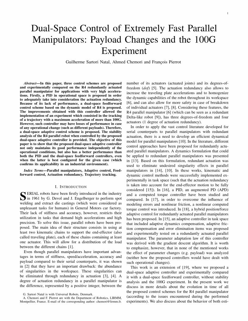
The R4 robot is a redundantly actuated parallel manipulatordesigned to have the capability of reaching 100G of acceler-ation. During its design, an optimization study was made inorder to identify the best configuration of its structure in orderto achieve such objective [6]. The most important variablesthat were taken into consideration in this optimization processwere the maximum achievable accelerations and the total costsof the components of this robot. From this analysis, it wasconcluded that the best structure which would provide theoptimal relation between acceleration capabilities and costwould have 4 actuators and 3 degrees of freedom (redundantlyactuated, cf. Fig. 1). This robot has a workspace of at leasta cylinder of 300 mm radius and 100 mm height, and eachof its four actuators (ETEL motor, model RTMB0140-100[21]) has a maximum torque of 127 N.m. Its CAD schematicview and side view are shown in Fig. 1. The platform of therobot (with and without a payload of 200g) is shown in Fig.2. Its geometrical parameters are summarized in Table I andillustrated in Fig. 3, and its dynamics parameters are describedin Table II.
XY
Z
4 ACTUATORS
3-DOF
Fig. 1. Views of the R4 parallel manipulator: Schematic view of the CADdesign (left), side view of the robot prototype (right)
Fig. 2. View of the platform (traveling plate) of the R4 parallel manipulator:without payload (left), with a payload of 200g (right)
B. Simplified Forward Dynamics
During the design phase of R4 parallel manipulator, somesimplifications were made in the dynamic model computation.These simplifications were based on the following hypotheses:• the joint frictions were neglected, as the components of
the robot were designed such that they would have verysmall frictions between them,
• the inertia of the forearms was also neglected, and theirmasses were split up into two parts each being artificiallyconsidered to be located at both ends of the forearms (halfof the mass is transferred to the end of the arm (Ai),whereas the other half is transferred to the traveling plate(Bi)),
• gravity acceleration was neglected since the case studiesconsidered very high accelerations, and the integral partof the controller is fast enough to compensate it.
These assumptions are discussed in more details in [6] and[22]. The final expression of the robot’s simplified forwarddynamic model is derived from a combination of the armsand the traveling plate equilibriums, and is given by [6]:
X = (MT + JmT ITJm)−1JTm(τ − IT JmX) (1)
where X ∈ Rm and X ∈ Rm are the vectors ofCartesian velocities and accelerations; MT = Diag{Mtp +
nMforearm
2 }m×m = MtotIm×m is a diagonal mass matrix,being Mtp the mass of the traveling plate, Mforearm the massof the forearm, Mtot the scalar value of the diagonal of MT ,m = 3 the number of degrees-of-freedom and n = 4 thenumber of motors; IT = Diag{Iact + Iarm}n×n = ItotIn×nis a diagonal matrix with n diagonal terms, where Iact andIarm are the inertia of the actuators and the inertia of the
3
Fig. 3. Illustration of the R4 parallel manipulator geometric parameters(detailed in Table I): Top view (left), side view (right)
TABLE IGEOMETRIC PARAMETERS OF R4 PARALLEL MANIPULATOR
rb [m] rtp [m] li [m] Li [m]0.135 0.05 0.2 0.53
arms, respectively, and Itot is the scalar value of the diagonalelements of IT ; Jm ∈ Rn×m and Jm ∈ Rn×m are respectivelythe generalized inverse Jacobian matrix and its first derivative;τ ∈ Rn represents the torques vector generated by theactuators. For further details on the mechanical design of theR4 parallel manipulator, the reader is referred to [6].
C. Actuation redundancy and its effects on control
Even though the actuation redundancy is a good solutionto deal with the singularities of a parallel manipulator in itsworkspace and to provide advantages in terms of mechanicalcapabilities of the robot, it creates a new issue in terms ofcontrol: classical articular control schemes are unable to dealwith dynamic effects in Cartesian space, and the integral termof a linear PID controller will be disturbed by kinematicinconsistencies.
0 0 0
Fig. 4. Illustration of actuation redundancy: Non-redundant case (left) andredundantly actuated case (right)
This concept is illustrated in Fig. 4. Consider, for instance,a system with one dof in the Cartesian space (end-effectoron the horizontal axis). In the first case, a linear actuator(on the vertical axis) is added to control the position of thisend-effector. This means that the system is not redundantlyactuated (in this example, it has one measuring scale in jointspace and one dof in the Cartesian space). Thus, it is alwayspossible to converge to a zero joint space error (which hasa “0” mark). In the second case, a second linear actuator isadded. The system has now two measuring scales in joint spaceand one dof in the Cartesian space, which means that it isredundantly actuated. By analyzing Fig. 4, it is possible tosee that any geometric error (due to machining inaccuracies,
TABLE IIDYNAMICS PARAMETERS OF R4 PARALLEL MANIPULATOR
Mtp [kg] Mforearm [kg] Iact [kg.m2] Iarm [kg.m2]0.2 0.065 0.003 0.005
assembly errors, backlash, thermal expansion, etc.) will makeit impossible to get all the measuring scales to reach a zeroerror at the same time. Thus the joint space error vector willnever be zero, and this error will always have an effect on theintegral term of the controller.
III. PROPOSED CONTROL SCHEMES: FROMCARTESIAN PID TO DUAL-SPACE ADAPTIVE
CONTROLA. PID controller in the Cartesian space
The first proposed control scheme experimentally imple-mented on the R4 parallel manipulator was the PID in opera-tional space. The main objective of this controller was to takeinto consideration the actuation redundancy of the manipulator.If such characteristic is not considered in the controller design,important internal forces may arise, compromising not onlythe performance of the system, but also the safety of itsmechanical structure. This control scheme is illustrated in Fig.5.
PID c I.K. -‐ MANIPULATOR
+ Xd qd
q
Δq ΔX F q
Fig. 5. Block diagram of the proposed Cartesian PID controller
The desired trajectory Xd is given in the Cartesian space.As only the joint positions are measured, this trajectory isconverted to the joint space through the inverse kinematics(I.K. block in Fig. 5) of the robot [6], such that the correspond-ing tracking error ∆q is computed in joint space. The jointtracking error must then be reconverted to its equivalent ∆Xin Cartesian space in order to be used in the PID controller.As the joint tracking errors ∆q are assumed to be significantlysmall, since the sampling time ∆t is of only 0.1ms (10−4s),let ∆q
∆t 'dqdt . If this robot were not redundantly actuated, this
conversion would be made by using ∆X ' J−1m ∆q, where
Jm ∈ Rn×m is the generalized inverse Jacobian matrix (whichmaps the traveling plate velocity vector X to the joint velocityvector q), being n the number of actuators and m the numberof dof of the robot. When the robot is not redundant, Jm is asquare matrix (n = m), therefore it can be inverted. However,in the case of R4, which has 4 actuators (n = 4) and 3 dof(m = 3), Jm cannot be inverted. The solution is then to usethe pseudo-inverse as follows:
∆X = H∆q (2)
being H the pseudo-inverse of Jm, that is H = J+m =
(JmTJm)−1Jm
T . It is worth mentioning that the pseudo-inverse applies as the Jacobian is not singular. The followingcontrol law is then proposed:

4
τ = HTF (3)
where F = (Kpec(t) + Ki
∫ec(t)dt + Kd
dec(t)dt ) is the force
applied on the traveling plate, ec = ∆X , and Kp, Ki and Kd
are the PID feedback gains.
B. The dual-space feedforward controller
When considering the dynamics of R4 parallel manipulator(1), a dual-space feedforward controller was proposed. Thiscontroller consists basically in a PID in the operational spaceaugmented with a feedforward of both desired Cartesian andarticular accelerations to improve its tracking performance.This control approach is illustrated in Fig. 6, and detailed asfollows.
PID c I.K. +
-‐ MANIPULATOR + + +
+
d² dt²
d² dt²
Xd qd
q
Δq ΔX F
Xd ..
qd ..
q
Fig. 6. Block diagram of the proposed dual-space feedforward controller
As will be shown in the sequel, the dual-space feedforwardcontroller was chosen because the dynamics of the system (1)can be rewritten in such a way that it will only be necessaryto add two feedforward terms (the Cartesian and joint desiredaccelerations) to the Cartesian PID in order to improve itstracking performance. A computed torque was not consideredhere because it would require the computation of the wholedynamics of the system (instead of using the much simplerrewritten form to be presented as follows), which is prohibitivefor an application which demands such small sampling time,even more if one considers that an adaptive process is to beadded to the control law.
1) Computation of the feedforward gains: In order to definethe feedforward gains of the dual-space controller, it is nec-essary to take into consideration the dynamics of the system(1). By multiplying its both sides by (MT + Jm
T ITJm), oneobtains:
(MT + JmT ITJm)X = Jm
T (τ − IT JmX) (4)
which results in:
MT X + JmT ITJmX = Jm
T τ − JmT IT JmX (5)
The torques term τ is isolated on the left side, and thefollowing expression is obtained:
JmT τ = MT X + Jm
T ITJmX + JmT IT JmX (6)
Both sides are then multiplied by the pseudo-inverse of JmT
(which will be named HT ):
τ = HTMT X + IT (JmX + JmX) (7)
where JmX + JmX = q. Then (7) can be rewritten as:
τ = HTMT X + IT q (8)
By direct analysis of Fig. 6 and Eq. (8), it is clear thatthe nominal values of the gains that should multiply Xd
and qd are, respectively, Kffc = Mtot and Kffa = Itot,as MT = MtotIm×m and IT = ItotIn×n. When goodvalues of these parameters are chosen for a specific case, agood tracking performance is expected. However, when anoperational change occurs (such as a change of load), animportant loss of performance can then be expected, becausethese gains will not be automatically updated accordingly tothese changes.
This issue may even be prohibitive for the utilization of suchcontroller in an industrial application with possible changes inthe robot environment, if one considers, for instance, pick-and-place tasks where a fast movement without payload is followedby another fast movement with an unknown payload. In orderto deal with such issue, a dual-space adaptive controller isproposed. It is detailed in the following.
C. Dual-space adaptive controller
The proposed dual-space adaptive control scheme is basedon the dual-space feedforward controller, presented above, andthe adaptive control scheme proposed in [20]. The most im-portant characteristic of this control approach is its capabilityof taking into consideration the dynamics of the system andestimate its parameters automatically in real-time. Considerthe general Lagrangian dynamic model [23], [24] of robotmanipulators in the matrix form:
I(q)q + C(q, q)q +G(q) + f(q, q) = τ (9)
where I(q) ∈ Rn×n is the inertia matrix, C(q, q)q ∈ Rn×1 isthe vector of Coriolis and centrifugal forces, G(q) ∈ Rn is thegravity vector and f(q, q) ∈ Rn is the vector of friction forcesand τ ∈ Rn represents the torques generated by the actuators.The general expression of the proposed control scheme isgiven as follows:
τ = I(q)qd + C(q, q)qd + G(q) +Kpej +Kdej (10)
where ej = qd − q, being ej its first derivative, I , C, G arethe estimates of I , C and G, respectively. Considering therewritten dynamics of the R4 manipulator (8), we propose toexpress (9) in dual-space. Then, the following control law isproposed:
τ = HT MtotXd + Itotqd +Kpej +Kdej (11)
which can be rewritten in operational space as:
F = Y θ +Kpcec +Kdcec (12)
where Kpc and Kdc are positive feedback gains, ec = Xd−X ,ec = Xd − X , and:
Y =[I3×3Xd JTmI4×4qd
]; θ =
[Mtot
Itot
](13)
being Y and θ the regressor vector and the vector of estimatedparameters, respectively, and I3×3, I4×4 are introduced onlyto emphasize the size of the involved vectors and matrices, not

5
influencing the actual calculations. These estimated parametersvary according to the following adaptation rule [20]:
˙θi =
γiiφi, if ai < θi < bi orθi ≥ bi and φi ≤ 0 orθi ≤ ai and φi ≥ 0
γii(1 +bi − θiδ
)φi, if θi ≥ bi and φi ≥ 0
γii(1 +θi − aiδ
)φi, if θi ≤ ai and φi ≤ 0
(14)
where• θi represents the estimate of the ith parameter,• γii is the ith element of the diagonal adaptation gain
matrix γ,• ai and bi are the lower and upper bounds of each
estimation, respectively,• φi is the ith element of the column matrix φ = Y T s;
being s = ec + λec, and λ(ec) = λ0
1+||ec|| , where λ0 is apositive constant,
• δ is a positive constant.The chosen adaptive gains were γ11 = 0.2 and γ22 =
1.5x10⁻⁴. These values were chosen such that the convergenceof the estimated parameters could be achieved quickly enoughfor a very fast pick-and-place task, and such that it wouldnot be aggressive enough to negatively affect the trajectorytracking performance of the manipulator. Considering an apriori knowledge of the mass (with a maximum payload ofaround 400g) and inertia of the robot, considering that the bestKffc gain of the feedforward controller was 0.625 for the casewithout payload and 0.825 for the case with a payload of 200g,and taking into account that bigger payloads might be used infuture experiments, the chosen range for the parameter Mtot
was of [0.525; 1] kg, which means a1 = 0.525 and b1 = 1. Theinertia parameter Itot, which is equivalent to the feedforwardgain Kffa, the range was chosen as [0.006, 0.018] kg.m2,which means a2 = 0.006 and b2 = 0.018. In this case study,one concentrates more on the behavior of the parameter Mtot,as this is the parameter that directly compensates for the loadchanges.
This adaptive control scheme is summarized in the blockdiagram of Fig. 7, where d
dt represents the direct derivation of∆X . The direct derivation is considered in this case because ofthe high resolution encoders that are used to measure the jointpositions, as well as because of the very small sampling period(which allows the generation of smooth derivative signals).D. Stability analysis
For the stability analysis of the parallel manipulator mod-eled by (1), subject to bounded disturbances (||d(t)|| ≤ dmax),in closed-loop with the dual-space adaptive controller (12)with adaptation law (14), the following assumptions are con-sidered:• ||θ(0)|| ≤ Θ, where Θ = {θ | ai ≤ θi ≤ bi, 1 ≤ i ≤p}, being ai and bi the chosen lower and upper boundsfor each estimated parameter θi and p the number ofestimated parameters,
Fig. 7. Block diagram of the proposed dual-space adaptive controller
• θ(t) ≤ Θδ , where Θ = {θ | ai − δ ≤ θi ≤ bi + δ, 1 ≤i ≤ p}, for some δ > 0,
• Xd, Xd and Xd, as well as qd, qd and qd are bounded,• the Jacobian and its inverse exist and are bounded by a
known constant J ∈ R+ such that ||Jm(η)||, ||J−1m (η)|| ≤
J . The minimum singular value of Jm(η) is assumedto be greater than a known small positive constant ϑ >0, such that Max{||J−1
m (η)||} is known a priori, andhence, all kinematic singularities are avoided. The time-derivative of the Jacobian (Jm) is also assumed to bebounded. These assumptions are valid if one considersthat the robot remains far from singularities [10].
Under these assumptions, the following theorem is pro-posed.
Theorem 1:The Cartesian error eTss = [eTc eTc ] will exponentially
converge to the following residual domain:
||ess||2 ≤ O(dmax
λλmin(Q)) +O(
1
γs) (15)
where γs represents the adaptation gain (by commodity, weconsidered that Γ = γsP , being Γ the adaptation gain matrixand P a positive definite diagonal matrix) and Q is given by[11]:
Q =
[||Kpc|| 1
2(||Kdc|| + 3
2ρ1||M ||)
12(||Kdc|| + 3
2ρ1||M ||) ||Kdc||
2λ0
](16)
being ρ1 the upper bound of the desired velocity and ||M || =||Mq(v)||, where Mq(v) = (vT ⊗ I)DqM
s(q), for any vectorv, is the vectorial representation of the partial derivative ofMs = Meq(q, q)− Ceq(q, q) with respect to q obtained fromChristoffel symbols Υ as follows:
Υ = λeT1 (Meq − Ceq)e2 =1
2λeT1 (M(x2)e2−
−M(e2)x2 − M(x2)T e2) (17)
with x2 = X , e1 = ec and e2 = ec.Proof:
In order to analyze the stability of the redundantly actuatedparallel manipulator in closed-loop with the proposed dual-space adaptive controller, let us firstly consider its dynamics,recalled below:
(Mtot + JTmItotJm)X + JTmItotJmX = JTmτ (18)

6
which can be rewritten as:
Meq(q)X + Ceq(q, q)X = F (19)
or, equivalently to [11] in operational space, as:{x1 = x2
x2 = −M−1eq (Ceqe2 − F )
(20)
where x1 = X , x2 = X , Meq = (Mtot + JTmItotJm) andCeq = JTmItotJm. It is now important to recall the appliedcontrol scheme:
F = MtotXd + JTmItotqd +Kpcec +Kdcec (21)
and then convert it to the Cartesian space (considering thatqd = Jm(qd, Xd)Xd+Jm(qd, qd, Xd, Xd)Xd, then adding andsubtracting Jm(q,X)Xd + Jm(q, q,X, X)Xd), gives:
F = MeqXd+CeqXd+JTmItot(JXd+ ˙JXd)+Kpcec+Kdcec(22)
where J = Jm(qd, Xd) − Jm(q,X) and ˙J =Jm(qd, qd, Xd, Xd) − Jm(q, q,X, X), which will beconsidered as a bounded disturbance to the controlledsystem (to be detailed later in the analysis). Firstly, theanalysis will be made while considering no disturbanceto the controlled system. Therefore, the control scheme inoperational space will be initially considered as follows:
F = MeqXd+CeqXd+Kpcec+Kdcec = Y θ+Kpcec+Kdcec(23)
As it was shown in [11], a system of the form (20) controlledby (23) with the adaptation law (14) is stable and convergesto:
||ess|| → 0 (24)
where eTss = [eTc eTc ]. This means that, without disturbance,both the position and velocity tracking errors will convergeto zero as time tends to infinity. However, the real system isdisturbed by:
d(t) = JTmItot(JXd + ˙JXd) (25)
This disturbance is bounded, because:• The robot configuration is assumed to be far from
the actuation singularities [10]. Therefore, Jm(q,X)and Jm(q, q,X, X) are bounded [15]. If one consid-ers that J = Jm(qd, Xd) − Jm(q,X) and ˙J =Jm(qd, qd, Xd, Xd)−Jm(q, q,X, X) and that Jm(qd, Xd)and Jm(qd, qd, Xd, Xd) are bounded, it is possible toconclude that J and ˙J are also bounded,
• Itot is bounded because of the projection of the estimatedparameters in the adaptive law,
• Xd and Xd, as well as qd and qd are bounded (adequatelychosen reference trajectories).
Let us then substitute the proposed control scheme (23) withadaptation law (14) into the dynamic model of the robot (19)while considering the bounded disturbance d(t). This resultsin:
MeqXd + CeqXd +Kpcec +Kdcec + d(t) = MeqX + CeqX(26)
By adding and subtracting MeqXd + CeqXd, one gets to:
Meq ec + Ceq ec + (Meq −Meq)Xd + (Ceq − Ceq)Xd+
+Kpcec +Kdcec + d(t) = 0(27)
which can be rewritten as:
Meq ec + Ceq ec = −Y θ −Kpcec −Kdcec − d(t) (28)
where Y = [Xd Xd] and θ = [MTeq C
Teq]
T , being Meq =
Meq −Meq and Ceq = Ceq − Ceq . Therefore, the expressionof the error dynamics can be written in state-space as follows:{
e1 = e2
e2 = −M−1eq (Ceqe2 +Kpce1 +Kdce2 + Y θ + d(t))
(29)
where e1 = ec and e2 = ec. Consider, as in [11], the followingLyapunov candidate (without disturbances):
V (t) =1
2eT1 Kpce1 +
1
2eT2 Meqe2 +λ(e1)eT1 Meqe2 +
1
2θTΓ−1θ
(30)being λ(e1) = λ0
1+||e1|| , where λ0 is a positive constant. ThisLyapunov candidate is guaranteed to be positive definite witha sufficiently small choice of λ0, and can be rewritten as:
V (t) =1
2eTss
[Kpc λMeq
λMeq Meq
]ess +
1
2θTΓ−1θ (31)
with ess = [eTc eTc ]T . The objective is now to evaluate thetime-derivative of V (t), which is given by:
V (t) = eT1 Kpce2 + eT2 Meq e2 +1
2eT2 Meqe2+
+ λeT2 Meqe2 + λeT1 Meq e2 + λeT1 Meqe2+
+ λeT1 Me2 + θTΓ−1 ˙θ
(32)
Considering that e2 = −M−1eq (Ceqe2+Kpce1+Kdce2+Y θ)
and also the skew-symmetry property of the matrix (Meq
2 −Ceq), one gets to:
V (t) = −eT2 (Kdce2 + Y θ) + λeT2 Meqe2 − λeT1 (Ceqe2+
+Kpce1 +Kdce2 + Y θ) + λeT1 Meqe2+
+ λeT1 Me2 + θTΓ−1 ˙θ
(33)
which will be represented as:
V (t) = ξ1 (34)
where ξ1 represents the right-hand side of (33). For such acase, considering [11], we can conclude that:
V (t) ≤ −λλmin(Q)||ess||2 (35)
where λmin(Q) represents the minimum eigenvalue of Q and:

7
Q =
[λmin(Kpc)
12(||Kdc|| + 3
2ρ1||M ||)
12(||Kdc|| + 3
2ρ1||M ||) λmin(Kdc)
2λ0
](36)
being ρ1 the upper bound of the desired velocity and Mq(v) =(vT ⊗ I)DqM
s(q), for any vector v, as previously defined.When considering the disturbance, the following expressionof the time-derivative of V (t) is obtained:
V (t) = −eT2 (Kdce2 + Y θ + d(t)) + λeT2 Meqe2−− λeT1 (Ceqe2 +Kpce1 +Kdce2 + Y θ+
+ d(t)) + λeT1 Meqe2 + λeT1 Me2 + θTΓ−1 ˙θ
(37)
which is equivalent to:
V (t) = ξ1 − (||eT2 + λeT1 ||)d(t) (38)
As d(t) can be negative, the conclusion for this stabilityanalysis is written as follows:
V (t) ≤ −λλmin(Q)||ess||2 + (||eT2 + λeT1 ||)dmax (39)
It is clear that, in the present case, it is not possible toguarantee that V (t) is negative definite. However, it is possibleto manipulate λmin(Q) (by carefully choosing Kpc, Kdc andλ0) such that the region where V (t) is positive can be madeas small as possible, therefore guaranteeing that the systemerror will converge to a residual domain that can be made assmall as possible (when not considering the saturation of theactuators).
This is illustrated in Fig. 8 for the example that follows (with||ess||2 = e2
1 + e22). Firstly, let us consider that λ = 0.01 and
λmin(Q) = 100 (configuration 1), and then consider that λ iskept with the same value and λmin(Q) = 300 (configuration2). In both cases, dmax = 5. It is possible to notice, asillustrated in Fig. 8, that by only increasing Kpc and Kdc
(thus increasing λmin(Q)), the Lyapunov candidate V (t) willconverge to a considerably smaller residual domain. This isbecause the increase of ||ess||2, after a certain point, willcause the time-derivative of V (t) to become negative. As theLyapunov candidate V (t) also depends directly on ||ess||2 (cf.the two first terms of (30)), this means that ||ess||2 will alsodecrease after this point. Finally, one must consider that theprojection of the estimated parameters (14) is not necessary inthe case without disturbances. However, in our case we havedisturbances, which generates the need for a projection in theadaptation algorithm (in order to guarantee the boundedness ofthe estimated parameters). This projection may add a residualerror to the controlled system which is inversely proportionalto the adaptation gain [12]. This leads to the conclusion that:
||ess||2 ≤ O(dmax
λλmin(Q)) +O(
1
γs) (40)
0 2 4 6 8 10 12 14 16
−2
−1
0
1
2
3
4
||ess
||2
V
Configuration 1Configuration 2
Fig. 8. Illustration of the effect of the increase of λmin(Q) on the behaviorof V (t) with respect to ||ess||2
IV. TRAJECTORY GENERATION
In this section, two proposed trajectories will be presentedand detailed. The first one consists in a spiral movement (cf.Fig. 9) that was implemented for a maximum accelerationof 20G (≈ 200m/s2, which provides a frequency of 6.5revolutions per second). This trajectory was used as a casestudy to compare the PID controller in operational space andthe dual-space feedforward controller. The second one consistsin a 3D pick-and-place trajectory as illustrated in Fig. 10. Thistrajectory was implemented for a maximum acceleration of30G with the dual-space feedforward controller as well as thedual-space adaptive controller.
A. First proposed trajectory: Spiral movements in x-y plane
The desired x-y trajectory is described as follows:{xd = Kmod 0.125 sin(2πfmovt)
yd = Kmod 0.125 sin(2πfmovt+π
2)
(41)
being Kmod = 0.5 sin( 2πt15 + 11π
10 ) a modulation functionthat guarantees a smooth variation of the circle’s radius inorder to avoid abrupt start/finish movements and fmov thefrequency of the circular movements (in Hz). The obtainedcurve is illustrated in Fig. 9. The associated experiment hasthe following procedure:
• the robot goes to its initial position (0, 0,−0.55)m andstops,
• the robot starts moving while the radius of the circularmovement increases smoothly until it reaches 0.125m andthen decreases smoothly until the robot stops.
The objective of this case study is to evaluate the track-ing performance that would be obtained by the addition ofthe desired Cartesian/joint acceleration feedforwards to theCartesian PID controller. As will be detailed in Section V,this performance improvement allowed for a safer increase ofthe acceleration/velocity of the robot until 30G, which wasachieved on the second proposed trajectory.

8
−0.1 −0.05 0 0.05 0.1
−0.1
−0.05
0
0.05
0.1
X (m)
Y (
m)
Fig. 9. Top view of the reference trajectory used in the first case study (spiralin the x-y plane)
B. Second proposed trajectory: 3D pick-and-place movements
The objective of this trajectory is to evaluate the capabilityof the proposed control schemes to deal with very highaccelerations/velocities in a pick-and-place task. The desiredtrajectory was chosen such that movements of different dis-tances would have to be performed in the same amount oftime. This would require different accelerations/velocities foreach one of them, demonstrating the good applicability ofthe proposed dual-space control schemes. The trajectory inquestion has the following sequence of movements:
1) Pick 1 - Place 1: From (-0.1,0.1)m to (0.1,-0.1)m,2) Place 1 - Pick 2: From (0.1,-0.1)m to (0.1,0.1)m,3) Pick 2 - Place 2: From (0.1,0.1)m to (-0.1,-0.1)m,4) Place 2 - Pick 1: From (-0.1,-0.1)m to (-0.1,0.1)m.
Each movement was performed in 0.08s without payload(0.32s for the whole cycle), and in 0.1s with payload (0.4sfor the whole cycle). Their maximum height was equal to2.5cm.
1
2
3
4
PICK 1
PICK 2
PLACE 1
PLACE 2
Fig. 10. Isometric view of the 3D pick-and-place trajectory
The trajectory generation algorithm used in this case wasa polynomial interpolation of degree five [25]. This algorithmguarantees the continuity of the movement in position, velocityand acceleration. The idea is to reach a desired final positionfrom a given initial position through the following function:
xf = xi + r(t)∆x, for 0 ≤ t ≤ tf (42)where
r(t) = 10(t
tf)3 − 15(
t
tf)4 + 6(
t
tf)5 (43)
being xi, xf the initial and final positions, respectively, r(t)a function that represents the trajectory between the twopositions (being its limits equal to r(0) = 0 and r(tf ) = 1),∆x = xf − xi and tf the duration of the movement (chosenby the user).
C. Third proposed trajectory: 100G vertical movements
In order to accomplish the objective of reaching 100G ofacceleration, a vertical trajectory (centered on the origin ofthe x-y plane) was proposed. This trajectory was proposedbecause the torques would be equally divided between the fouractuators, and also because of the symmetrical internal effortsto be supported by the structure of the robot. This trajectoryis described by an expression similar to the one of the spiraltrajectory, but only on the z axis in this case:
zd(t) = Kmod 0.05 sin(2πfmovt) (44)being Kmod the same modulation function of the spiraltrajectory used in Section IV-A to avoid an abrupt start/finishof the movements, and fmov the frequency of the sinusoidalmovement (in Hz), being fmov = 22Hz. The desired trajec-tory is illustrated in Fig. 15. The associated experiment hasthe following procedure:• the robot is steered to its initial position (0, 0,−0.55)m
and stops (initialization),• the amplitude of the movement increases smoothly until
it reaches 0.05m and then decreases smoothly until therobot stops.
V. REAL-TIME EXPERIMENTAL RESULTS
In this section, real-time experimental results obtainedthrough the application of the proposed control schemes de-scribed in Section III on the parallel manipulator R4 describedin Section II in order to track the reference trajectories detailedin Section IV are presented and discussed.
TABLE IIIPARAMETERS OF THE CARTESIAN PID CONTROLLER
Kp Ki Kd8000 600 40
TABLE IVPARAMETERS OF THE DUAL-SPACE FEEDFORWARD CONTROLLER
Kp Ki Kd Kffc Kffa8000 600 40 0.625/0.825 0.012

9
TABLE VCONFIGURATION OF THE DUAL-SPACE ADAPTIVE CONTROLLER
Adaptive gains γ11 = 0.2 / γ22 = 1.5e−4
Range of Mtot (kg) [0.525;1]Range of Itot (N.m) [0.006;0.018]
λ0 100δ 0.0001Kp 8000Kd 40
A. Description of the experimental testbed
The proposed control schemes were implemented inSimulink/Matlab of Mathworks, being compiled using XPCTarget real-time toolbox, and uploaded to the target PC,which managed the real-time task execution with a samplingfrequency of 10 kHz (sampling period of 0.1msec). Becauseof such high sampling frequency, the utilization of externalmeasurement devices such as cameras for the measurement ofthe position of the platform was not considered. The positionof the platform was calculated through the forward kinematicsof the robot, and the Cartesian velocity was obtained throughdirect derivation of the calculated Cartesian position. Theexperimental testbed of our prototype is displayed in Fig. 11,where:
3 2
1
4
Fig. 11. View of the experimental testbed of R4 parallel manipulator
• the PC used for the development of the control schemesin Simulink/Matlab is represented by item 1©,
• the dedicated target PC, responsible for the real-timecontrol of the robot, is represented by item 2©,
• the emergency stop button is represented by item 3©,• the R4 parallel manipulator is represented by item 4©.Four main experimental scenarios are proposed and imple-
mented on this testbed, namely:1) comparison between PID and dual-space feedforward
controllers,2) 100G experiment with the dual-space feedforward con-
troller,3) dual-space feedforward controller overall performance
analysis,
4) comparison between dual-space feedforward and adap-tive controllers.
Each of these scenarios is detailed and discussed in thesequel.
B. Comparison between the Cartesian PID and the dual-spacefeedforward controller
Based on this experiment, a first comparison will be madebetween the Cartesian PID and the dual-space feedforwardcontroller for the case of the spiral trajectory in the x-y plane for a maximum acceleration of 20G (equivalentto fmov = 6.5Hz). This trajectory was selected for thiscomparison because it is relatively simple both in terms ofthe dynamics involved and also because of the symmetry ofthe movements. The obtained results for this scenario aregiven in Figs. 13-14. In Fig. 12, the movement along x-axis(similar for y-axis, with a delay of 90◦) is illustrated. Duringits initialization, the robot goes from the rest position to thedesired initial position (0, 0,−0.55)m, then the amplitude ofthe circle starts to increase until it reaches 0.125m (reachinga maximum acceleration of 20G), and then it decreases inthe same way until the robot stops. In order to compare theperformance of both controllers, Figs. 13-14 show a zoomaround the time interval of maximum amplitude.
0 5 10 15 20
−0.1
−0.05
0
0.05
0.1
t (s)
X (
m)
Fig. 12. View of the trajectory of the traveling plate along x-axis vs. time
By analyzing Fig. 13, it is possible to notice that the dual-space feedforward controller provides a better tracking perfor-mance than the classical Cartesian PID. The former is able tokeep the tracking errors within the interval [−1.55, 2.34]mm,while the latter keeps them within [−4.62, 5.33]mm. Thismeans that the dual-space feedforward controller provides apeak-to-peak (difference between the highest peak and thelowest valley of a signal) error improvement of approximately60%. The Root Mean Square Error (RMSE) can also beused to evaluate the tracking performance of the proposedcontrollers. The computation of the RMSE takes into consid-eration all the three axes equally, as detailed in the following:
erms =√e2rmsx + e2
rmsy + e2rmsz (45)

10
10.5 10.52 10.54 10.56 10.58 10.6 10.62 10.64−5
0
5x 10
−3e cX
(m
)
PIDDual Space
10.46 10.48 10.5 10.52 10.54 10.56 10.58 10.6−5
0
5
x 10−3
t (s)
e cY (
m)
Fig. 13. Evolution of the resulting tracking errors for the PID controller (solidline) and for the dual-space feedforward controller (dashed line)
10.46 10.48 10.5 10.52 10.54 10.56 10.58 10.6−30
−20
−10
0
10
20
30
t (s)
τ 1 (N
.m)
PIDDual Space
Fig. 14. Evolution of the torque of one actuator for the cases of the PIDcontroller (solid line) and the dual-space feedforward controller (dashed line)
where ermsx (and equivalently ermsy and ermsz ) is given by:
ermsx =
√e2x1
+ e2x2
+ ...+ e2xn
n(46)
where n is the total number of elements of ex. The RMSEshows an equivalent improvement in performance with thedual-space feedforward controller (1.3 mm versus 3.6 mm,which means an improvement of approximately 64%). Anotheradvantage of the dual-space feedforward controller was thatits control signal had a smaller peak-to-peak value thanthe Cartesian PID (as shown in Fig. 14). These results aresummarized in Table VI.
With the conclusion that the Cartesian PID controller has arelatively bad tracking performance even for a trajectory whichis relatively simple, the former was discarded for the next casestudy.
C. The 100G experiment
The trajectory tracking obtained with the dual-space feed-forward controller for the 100G vertical trajectory is displayedin Fig. 15 (where the steering from the rest position to thedesired initial position, as well as the natural descent of theend-effector (due to the gravity acceleration) after the motorsare turned off at the end of the experiment are illustrated).A zoom on the period around the maximum acceleration(maximum amplitude of the sinusoidal movement) for thetrajectory tracking and the torques are depicted in Figs. 16and 17. The torque×angular velocity relation for each motoris shown in Fig. 19.
0 5 10 15 20
−0.6
−0.58
−0.56
−0.54
−0.52
−0.5
t (s)
Z (
m)
Des. Traj.FF
Fig. 15. Trajectory tracking obtained with the dual-space feedforwardcontroller for the 100G vertical trajectory, including initialization phase
10.34 10.35 10.36 10.37 10.38 10.39 10.4 10.41 10.42 10.43−0.6
−0.58
−0.56
−0.54
−0.52
−0.5
t (s)
Z (
m)
Des. Traj.FF
Fig. 16. Zoom on the trajectory tracking obtained with the dual-spacefeedforward controller for the 100G vertical trajectory
From Fig. 16, it is possible to notice that the feedforwardcontroller is able to keep the system stable and with an accept-able tracking error (inside the interval of [−3.31, 3.88]mm,which is equivalent to a peak-to-peak error of approximately7.2%) even while tracking a trajectory with such high acceler-ation. By analyzing Fig. 17 (representing the evolution of the

11
10.34 10.35 10.36 10.37 10.38 10.39 10.4 10.41 10.42 10.43−100
−80
−60
−40
−20
0
20
40
60
80
100
t (s)
Tor
ques
(N
.m)
τ1
τ2
τ3
τ4
Fig. 17. Torques generated by the dual-space feedforward controller
Fig. 18. Mechanical limits of the motors of R4 parallel manipulator (3RBS)for Tp and Tc, namely peak torque and constant torque, respectively
0 100 200 300 400 500 6000
50
100
150
τ 1 (N
.m)
MeasuredLimit
0 100 200 300 400 500 6000
50
100
150
τ 2 (N
.m)
0 100 200 300 400 500 6000
50
100
150
τ 3 (N
.m)
0 100 200 300 400 500 6000
50
100
150
Speed (rpm)
τ 4 (N
.m)
Fig. 19. Illustration of the mechanical power admissibility of the actuatorsduring the 100G experiment vs. their mechanical limits
0 5 10 15 20−1000
−800
−600
−400
−200
0
200
400
600
800
1000
t (s)
Acc
eler
atio
n (m
/s2 )
Fig. 20. Evolution of the traveling plate Cartesian acceleration along thez-axis for the 100G trajectory
control inputs (torques)), one can see that the four actuatorshad a similar maximum amplitude and, from Fig. 19, one cansee that the the four motors are close to reaching their powerlimits (maximum torque of 127N.m and maximum speed of550rpm, as illustrated in Fig. 18 (Tp − 3RBS), which refersto the characteristics of the chosen motors). The motors weredesigned with a thermal protection system against overheating,in order to guarantee that high temperatures would not affecttheir performances [26]. Fig. 20 shows that the robot was ableto reach more than 100G of acceleration (which is equivalentto approximately 981m/s2 if one considers that the gravityacceleration is approximately 9.81m/s2) with the proposeddual-space feedforward controller. The peaks of 1000m/s2 areequivalent to around 102G of acceleration. The accelerationsof each axis were measured on R4 with a Silicon Designstriaxial analog accelerometer (Model 2460-200) attached toits end-effector.
In the sequel, we are interested in analyzing the performanceof the dual-space feedforward controller in details, especiallyits limitations for an application involving operational changes.
TABLE VIPERFORMANCE COMPARISON BETWEEN THE CARTESIAN PID AND THE
DUAL-SPACE FEEDFORWARD CONTROLLER
Performance PID Dual-spaceError peaks [−4.6, 5.3]mm (4%) [−1.5, 2.3]mm (1.6%)
RMSE 3.6 mm 1.3 mmControl signals Dual-Space has slightly smaller peak-to-peak value
D. Dual-space feedforward controller performance analysisIn order to check the capabilities of this control approach
and analyze its lack of robustness, the 3D pick-and-placetrajectory presented in Section IV is proposed to be trackedfor two scenarios. Firstly, the parallel manipulator R4 willtrack this trajectory without any payload at 30G of maximumacceleration, then it will be tracked with a payload of 200gat 20G of maximum acceleration. During initialization, therobot goes from the rest position to the desired initial po-sition (−0.1, 0.1,−0.55)m, then two cycles of the proposed
12
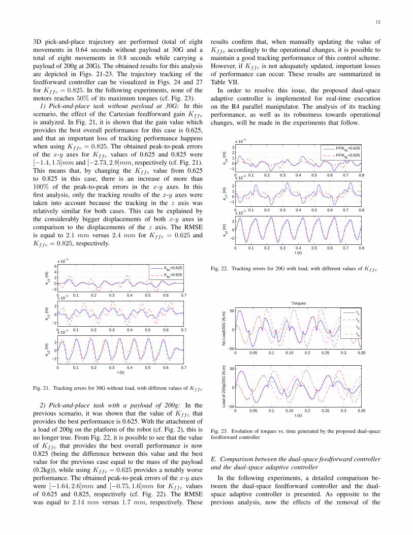
3D pick-and-place trajectory are performed (total of eightmovements in 0.64 seconds without payload at 30G and atotal of eight movements in 0.8 seconds while carrying apayload of 200g at 20G). The obtained results for this analysisare depicted in Figs. 21-23. The trajectory tracking of thefeedforward controller can be visualized in Figs. 24 and 27for Kffc = 0.825. In the following experiments, none of themotors reaches 50% of its maximum torques (cf. Fig. 23).
1) Pick-and-place task without payload at 30G: In thisscenario, the effect of the Cartesian feedforward gain Kffc
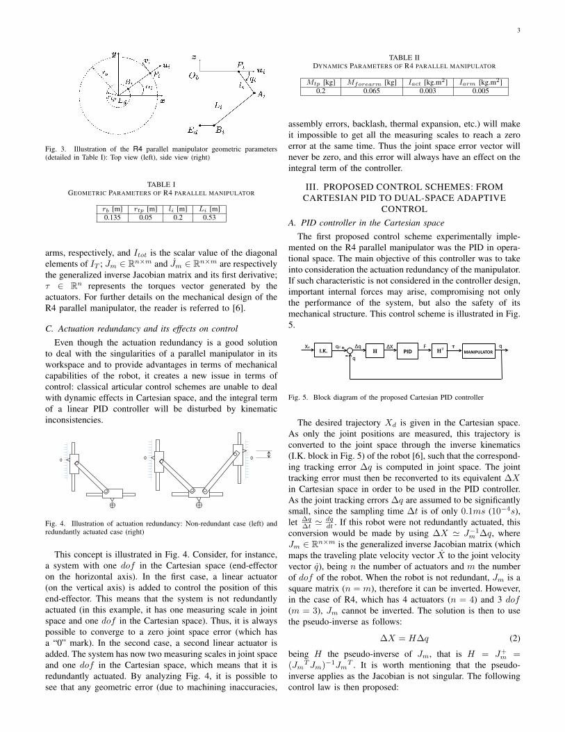
is analyzed. In Fig. 21, it is shown that the gain value whichprovides the best overall performance for this case is 0.625,and that an important loss of tracking performance happenswhen using Kffc = 0.825. The obtained peak-to-peak errorsof the x-y axes for Kffc values of 0.625 and 0.825 were[−1.4, 1.5]mm and [−2.73, 2.9]mm, respectively (cf. Fig. 21).This means that, by changing the Kffc value from 0.625to 0.825 in this case, there is an increase of more than100% of the peak-to-peak errors in the x-y axes. In thisfirst analysis, only the tracking results of the x-y axes weretaken into account because the tracking in the z axis wasrelatively similar for both cases. This can be explained bythe considerably bigger displacements of both x-y axes incomparison to the displacements of the z axis. The RMSEis equal to 2.1 mm versus 2.4 mm for Kffc = 0.625 andKffc = 0.825, respectively.
0 0.1 0.2 0.3 0.4 0.5 0.6 0.7
−2
0
2
4
6x 10
−3
e cX (
m)
0 0.1 0.2 0.3 0.4 0.5 0.6 0.7
−2
0
2
x 10−3
e cY (
m)
0 0.1 0.2 0.3 0.4 0.5 0.6 0.7
−2
0
2
x 10−3
t (s)
e cZ (
m)
Kffc
=0.625
Kffc
=0.825
Fig. 21. Tracking errors for 30G without load, with different values of Kffc
2) Pick-and-place task with a payload of 200g: In theprevious scenario, it was shown that the value of Kffc thatprovides the best performance is 0.625. With the attachment ofa load of 200g on the platform of the robot (cf. Fig. 2), this isno longer true. From Fig. 22, it is possible to see that the valueof Kffc that provides the best overall performance is now0.825 (being the difference between this value and the bestvalue for the previous case equal to the mass of the payload(0.2kg)), while using Kffc = 0.625 provides a notably worseperformance. The obtained peak-to-peak errors of the x-y axeswere [−1.64, 2.6]mm and [−0.75, 1.6]mm for Kffc valuesof 0.625 and 0.825, respectively (cf. Fig. 22). The RMSEwas equal to 2.14 mm versus 1.7 mm, respectively. These
results confirm that, when manually updating the value ofKffc accordingly to the operational changes, it is possible tomaintain a good tracking performance of this control scheme.However, if Kffc is not adequately updated, important lossesof performance can occur. These results are summarized inTable VII.
In order to resolve this issue, the proposed dual-spaceadaptive controller is implemented for real-time executionon the R4 parallel manipulator. The analysis of its trackingperformance, as well as its robustness towards operationalchanges, will be made in the experiments that follow.
0 0.1 0.2 0.3 0.4 0.5 0.6 0.7 0.8
−10123
x 10−3
e cX (
m)
0 0.1 0.2 0.3 0.4 0.5 0.6 0.7 0.8
−1012
x 10−3
e cY (
m)
0 0.1 0.2 0.3 0.4 0.5 0.6 0.7 0.8
−2
0
2
x 10−3
t (s)
e cZ (
m)
FF/Kffc
=0.625
FF/Kffc
=0.825
Fig. 22. Tracking errors for 20G with load, with different values of Kffc
0 0.05 0.1 0.15 0.2 0.25 0.3 0.35−50
0
50
No
Load
/30G
(N
.m)
Torques
τ1
τ2
τ3
τ4
0 0.05 0.1 0.15 0.2 0.25 0.3 0.35−50
0
50
t (s)
Load
of 2
00g/
20G
(N
.m)
Fig. 23. Evolution of torques vs. time generated by the proposed dual-spacefeedforward controller
E. Comparison between the dual-space feedforward controllerand the dual-space adaptive controller
In the following experiments, a detailed comparison be-tween the dual-space feedforward controller and the dual-space adaptive controller is presented. As opposite to theprevious analysis, now the effects of the removal of the

13
TABLE VIISUMMARY OF THE PERFORMANCE ANALYSIS OF THE PROPOSED
DUAL-SPACE FEEDFORWARD CONTROLLER FOR DIFFERENT VALUES OFKffc
Kffc = 0.625 Kffc = 0.825Error peaks (x-y, No load, 30G) [−1.4, 1.5]mm [−2.73, 2.9]mm
Error peaks (x-y, With load, 20G) [−1.64, 2.6]mm [−0.75, 1.6]mmRMSE (No load, 30G) 2.1 mm 2.4 mm
RMSE (With load, 20G) 2.14 mm 1.7 mm
payload will be evaluated. Therefore, the order of the scenarioswill be inverted (firstly, the performance of both controllers isevaluated and compared for the case with a payload of 200gat 20G, and then for the case without payload at 30G). Inboth scenarios, the robot goes from the rest position to thedesired initial position (−0.1, 0.1,−0.55)m and then executestwo cycles of the proposed 3D pick-and-place trajectory.
1) 3D pick-and-place movements with a payload of 200gat 20G: In this scenario, the adaptive controller is comparedto the feedforward controller (best configured for the casewith a payload of 200g, that is Kffc = 0.825), at 20G ofmaximum acceleration. The objective of this experiment is toshow that even though the feedforward controller may havea good performance when configured with its best value ofKffc for a specific scenario, it will still have a worse trackingperformance than the adaptive controller. The obtained resultsfor this scenario are depicted in Figs. 24-26.
0 0.05 0.1 0.15 0.2 0.25 0.3 0.35 0.4
−0.1
0
0.1
X (
m)
0 0.05 0.1 0.15 0.2 0.25 0.3 0.35 0.4−0.1
0
0.1
Y (
m)
0 0.05 0.1 0.15 0.2 0.25 0.3 0.35 0.4
−0.55
−0.54
−0.53
t (s)
Z (
m)
Des. Traj.AdaptiveFF/K
ffc=0.825
Fig. 24. 3D pick-and-place trajectory tracking with a payload of 200g for 1cycle and an acceleration of 20G
By analyzing Fig. 25, it is possible to notice that theadaptive controller is able to provide a better overall trackingperformance than the feedforward controller even with its bestconfiguration value of Kffc for this case. For the x-y axes, theadaptive controller is able to keep the tracking errors withinthe interval [−1, 1]mm, while the feedforward controller keepsthem within [−0.75, 1.6]mm, as shown in Table VIII. Forthe z-axis, the difference between the controllers is biggerand easily visible. While the adaptive controller keeps thetracking errors within [−1.77, 2]mm, the feedforward keepsthem within [−2.6, 2.7]mm. The superior performance of the
0 0.1 0.2 0.3 0.4 0.5 0.6 0.7 0.8
−5
0
5
10
15x 10
−4
e cX (
m)
0 0.1 0.2 0.3 0.4 0.5 0.6 0.7 0.8−1
0
1
x 10−3
e cY (
m)
0 0.1 0.2 0.3 0.4 0.5 0.6 0.7 0.8
−2
0
2
x 10−3
t (s)
e cZ (
m)
AdaptiveFF/K
ffc=0.825
Fig. 25. 3D pick-and-place tracking errors with a payload of 200g for anacceleration of 20G
0 0.1 0.2 0.3 0.4 0.5 0.6 0.7 0.8
−200
2040
τ 1 (N
.m)
AdaptiveFF/K
ffc=0.825
0 0.1 0.2 0.3 0.4 0.5 0.6 0.7 0.8−50
0
50
τ 2 (N
.m)
0 0.1 0.2 0.3 0.4 0.5 0.6 0.7 0.8−50
0
50
τ 3 (N
.m)
0 0.1 0.2 0.3 0.4 0.5 0.6 0.7 0.8−50
0
50
t (s)
τ 4 (N
.m)
Fig. 26. Torques applied by the 4 motors with a payload of 200g for anacceleration of 20G
0 0.05 0.1 0.15 0.2 0.25 0.3−0.1
0
0.1
X (
m)
0 0.05 0.1 0.15 0.2 0.25 0.3−0.1
0
0.1
Y (
m)
0 0.05 0.1 0.15 0.2 0.25 0.3−0.55
−0.54
−0.53
t (s)
Z (
m)
Des. Traj.AdaptiveFF/K
ffc=0.825
Fig. 27. 3D pick-and-place trajectory tracking without payload for 1 cycleand an acceleration of 30G

14
0 0.1 0.2 0.3 0.4 0.5 0.6 0.7
−2
0
2
4
x 10−3
e cX (
m)
0 0.1 0.2 0.3 0.4 0.5 0.6 0.7
−2
0
2
x 10−3
e cY (
m)
0 0.1 0.2 0.3 0.4 0.5 0.6 0.7
−2
0
2
x 10−3
t (s)
e cZ (
m)
AdaptiveFF/K
ffc=0.825
Fig. 28. 3D pick-and-place tracking errors without payload for an accelerationof 30G
0 0.1 0.2 0.3 0.4 0.5 0.6 0.7−40−20
02040
τ 1 (N
.m)
AdaptiveFF/K
ffc=0.825
0 0.1 0.2 0.3 0.4 0.5 0.6 0.7−50
0
50
τ 2 (N
.m)
0 0.1 0.2 0.3 0.4 0.5 0.6 0.7−50
0
50
τ 3 (N
.m)
0 0.1 0.2 0.3 0.4 0.5 0.6 0.7−50
0
50
τ 4 (N
.m)
Fig. 29. Torques applied by the 4 motors without payload for an accelerationof 30G
adaptive controller in this case is further confirmed by the RootMean Square Errors (RMSE), which are equal to 1.33 mmversus 1.7 mm for the feedforward controller. The RMSEtakes into consideration the errors in all axes equally. Theseresults are summarized in Table VIII.
The control inputs (torques) generated by each controller areshown in Fig. 26. It is worth to emphasize that all the controlinputs remain within the admissible limit of the actuators (amaximum torque of 127 N.m).
In the next scenario, it will be shown that the adaptivecontroller maintains its good performance without any needof manual readjustments of its parameters, while the dual-space feedforward controller loses much performance whennot updated accordingly.
2) 3D pick-and-place movements without payload at 30G:In this scenario, the robustness of the dual-space adaptive con-troller and the lack of robustness of the dual-space feedforwardcontroller towards load changes are demonstrated. From Fig.28, it is possible to notice that the feedforward controller,
TABLE VIIITRACKING PERFORMANCE OBTAINED WITH THE PROPOSED DUAL-SPACE
CONTROLLERS FOR A 20G PICK-AND-PLACE TRAJECTORY WITH APAYLOAD OF 200g
Performance Adaptive FF (Kffc = 0.825)Error peaks (x-y) [−1, 1]mm [−0.75, 1.6]mmError peaks (z) [−1.77, 2]mm [−2.6, 2.7]mm
RMSE 1.33 mm 1.7 mmControl Signals Smooth/far from limits
Adaptive controller: Slightly bigger amplitude
when not manually reconfigured to the new scenario, has animportant loss of performance (both with respect to the previ-ous scenario and also with respect to the adaptive controller).For the x-y axes, the adaptive controller keeps them within[−1.51, 1.6]mm, while the feedforward controller keeps themwithin [−2.73, 2.9]mm (peak-to-peak difference of more than80%). The robustness of the adaptive controller and the lack ofrobustness of the feedforward controller are further confirmedby the RMSE results. While the adaptive controller is able tomaintain almost the same RMSE as in the previous scenario(1.33 mm versus 1.4 mm), the feedforward controller had aloss of almost 40% (1.7 mm versus 2.4 mm), respectively.Fig. 29 confirms that the adaptive controller generates a controlsignal with a slightly bigger amplitude than the feedforwardcontroller. These results are summarized in Table VIII.
TABLE IXTRACKING PERFORMANCE OBTAINED WITH THE PROPOSED DUAL-SPACE
CONTROLLERS FOR A 30G PICK-AND-PLACE TRAJECTORY WITHOUTPAYLOAD
Performance Adaptive FF (Kffc = 0.825)Error peaks (x-y) [−1.51, 1.6]mm [−2.73, 2.9]mmError peaks (z) [−1.72, 1.84]mm [−2.26, 2.77]mm
RMSE 1.4 mm 2.4 mmControl Signals Smooth/far from limits
Adaptive controller: Slightly bigger amplitude
F. Variation of the estimated parameters
As already mentioned in Section III, the parameters Mtot
and Itot were estimated in real-time by the dual-space adaptivecontroller to maintain its good performance independently ofthe scenario. It was shown in this section that the adaptivecontroller outperforms the fixed feedforward controller evenwith its best settings for each scenario. The evolution of bothestimations will be detailed as follows.
For the first scenario, the value of Kffc (which will beconsidered as an offline estimation of Mtot) that providesthe best performance of the feedforward controller is equalto 0.825 (dashed curves in both Figs. 30-31). The first pointto be mentioned is that the convergence of the estimation ofMtot from a given initial value to a region around 0.825 isfast enough to be accomplished before the first stop pointis reached (which is the expected performance in a pick-and-place task, where the robot will perform a movementwith payload followed by a movement without payload). Thisconfirms the fact that the tracking performance of the adaptivecontroller will barely be affected by an initial value different

15
from the best value for the specific case, and also justifies thegood performance of the feedforward controller when keepingthis value constant during this experiment.
0 0.1 0.2 0.3 0.4 0.5 0.6 0.7 0.80.7
0.8
0.9
1
tmov
=0.15s (8G)
0 0.1 0.2 0.3 0.4 0.5 0.6 0.7 0.80.7
0.8
0.9
1
Mto
t(k
g)
tmov
=0.125s (12.5G)
0 0.1 0.2 0.3 0.4 0.5 0.6 0.7 0.8
0.7
0.8
0.9
1
t (s)
tmov
=0.1s (20G)
Fig. 30. Evolution of the estimated parameter Mtot (solid line) and the gainKffc (dashed line) for different accelerations (with a payload of 200g)
0 0.1 0.2 0.3 0.4 0.5 0.6 0.7
0.6
0.7
0.8
tmov
=0.125s (12.5G)
0 0.1 0.2 0.3 0.4 0.5 0.6 0.7
0.6
0.7
0.8
Mto
t(k
g)
tmov
=0.1s (20G)
0 0.1 0.2 0.3 0.4 0.5 0.6 0.70.5
0.6
0.7
0.8
t (s)
tmov
=0.08s (30G)
Fig. 31. Evolution of the estimated parameter Mtot (solid line) and the gainKffc (dashed line) for different accelerations (without payload)
For the second scenario, the important loss of performanceof the feedforward controller is justified. In Fig. 31, it is shownthat when not manually updating the feedforward gain Kffc
after the removal of the payload of 200g, this estimation willnow remain constant with an inadequate value. The estimationof the adaptive controller converges to a region around Mtot =0.625, which is the best value of Kffc for this case.
Another point to be mentioned is the increased oscillationsin parameters’ estimation with the increase of acceleration (cf.Figs. 30-33). Between the most reasonable causes, one canmention the increase of unmodeled dynamics effects (such asthe frictions, counter-electromotice forces, etc.), which becomemore important with higher accelerations, thus becoming arelevant disturbance source. However, the robustness of theadaptive controller enables it to maintain both smoothnessand good performance of the closed-loop system, in terms of
tracking (cf. Figs. 24,27), as well as in terms of evolution ofthe control inputs (the same general form for both controllers,without addition of oscillations by the adaptive controller, cf.Figs. 26,29), despite oscillations in the parameters’ estimation.It is worth mentioning, however, that the utilization of amore complete model may contribute to the decrease ofthese oscillations in the estimated parameters, as well as tothe improvement of the overall performance of the proposedadaptive controller. This shall be investigated in the future.
For instance, the evolution of Itot is displayed in Figs. 32-33 for different accelerations. From these figures, it is possibleto notice that the load changes had no significant effect on thebehavior of this parameter.
0 0.1 0.2 0.3 0.4 0.5 0.6 0.7 0.80.01
0.015
0.02
0 0.1 0.2 0.3 0.4 0.5 0.6 0.7 0.80.01
0.015
0.02
I tot
(kg.m
2)
0 0.1 0.2 0.3 0.4 0.5 0.6 0.7 0.8
0.01
0.015
0.02
t (s)
tmov
=0.15s (8G)
tmov
=0.125s (12.5G)
tmov
=0.1s (20G)
Fig. 32. Evolution of the estimated parameter Itot for different accelerations(with a payload of 200g)
0 0.1 0.2 0.3 0.4 0.5 0.6 0.70.01
0.015
0.02
0.025
0 0.1 0.2 0.3 0.4 0.5 0.6 0.70.01
0.015
0.02
0.025
I tot
(kg.m
2)
0 0.1 0.2 0.3 0.4 0.5 0.6 0.7
0.01
0.015
0.02
0.025
t (s)
tmov
=0.125s (12.5G)
tmov
=0.1s (20G)
tmov
=0.08s (30G)
Fig. 33. Evolution of the estimated parameter Itot for different accelerations(without payload)
VI. CONCLUSIONS AND FUTURE WORKIn this paper, three control schemes have been proposed
and experimentally compared on the R4 redundantly actuatedparallel manipulator for tasks with very high accelerations.A Cartesian PID controller was initially proposed such that

16
the redundancy in actuation would be taken into considerationin its design. Because of its limitation in terms of trackingperformance even with a relatively simple trajectory, a dual-space feedforward controller based on the dynamics of thesystem was proposed. The results showed that this last one canimprove the tracking performance considerably (even allowingthe execution of a 100G trajectory tracking experiment),but it has important losses of performance if there are anyoperational changes (such as load changes). To overcome suchlack of robustness, a dual-space adaptive controller was thenproposed. By analyzing the obtained experimental results fordifferent cases with and without payload, it was clear thatthis control scheme not only is able to maintain its goodperformance in both scenarios without any need of manualreadjustment of its parameters, but it also provides a betterperformance than the dual-space feedforward controller evenwhen this last one is best configured for each specific case.As future work, the utilization of a more complete dynamicmodel of R4 shall be analyzed, such that an evaluation ofthe possible performance improvements with the proposedadaptive control scheme can be made. Experiments with morecomplex trajectories for other applications such as laser cuttingshall also be studied.
VII. ACKNOWLEDGEMENTSThe authors would like to sincerely thank Prof. Liu Hsu
(COPPE/UFRJ, Brazil) for his valuable remarks and discus-sions for the development of the presented stability analysis.
REFERENCES
[1] J.-P. Merlet, “Parallel robots,” Kluwer Academic Publishers, 2000.[2] S. Kock and W. Schumacher, “A parallel x-y manipulator with actuation
redundancy for high-speed and active-stiffness applications,” Proc. IEEEConf. Rob. Autom., Leuven, Belgium, pp. 2295–2300, 1998.
[3] C. Gosselin and J. Angeles, “Singularity analysis of closed-loop kine-matic chains,” IEEE Trans. on Rob. Autom., vol. 6, no. 3, pp. 281–290,1990.
[4] F. C. Park and J. W. Kim, “Singularity analysis of closed kinematicchains,” ASME Trans. J. Mech. Des., vol. 121, no. 1, pp. 32–38, 1999.
[5] L. Ganovski, “Modeling, simulation and control of redundantly actuatedparallel manipulators,” PhD. dissertation, Universite Catholique deLouvain, Faculte des Sciences Appliquees, Belgique, 2007.
[6] D. Corbel, M. Gouttefarde, O. Company, and F. Pierrot, “Towards100g with pkm. is actuation redundancy a good solution for pick-and-place?,” Proc. of the IEEE Int. Conf. on Rob. and Autom., Alaska, USA,pp. 4675–4682, 2010.
[7] Y. Yi, J. E. Mcinroy, and Y. X. Chen, “Fault tolerance of parallelmanipulators using task space and kinematic redundancy,” IEEE Trans.Rob., vol. 22, no. 5, pp. 1017–1021, 2006.
[8] R. G. Roberts, H. G. Yu, and A. A. Maciejewski, “Fundamentallimitations on designing optimally fault-tolerant redundant manipulator,”IEEE Trans. Rob., vol. 24, no. 5, pp. 1224–1237, 2008.
[9] R. Clavel, “Delta, a fast robot with parallel geometry,” Int. Symp. onInd. Rob., Lausanne, Switzerland, pp. 91–100, 1988.
[10] H. Cheng, Y. K. Yiu, and Z. X. Li, “Dynamics and control of redundantlyactuated parallel manipulators,” IEEE Trans. Mech., vol. 8, no. 4,pp. 483–491, 2003.
[11] L. Whitcomb, A. Rizzi, and D. Koditschek, “Comparative experimentswith a new adaptive controller for robot arms,” IEEE Trans. on Rob.Autom., vol. 9, no.1, pp. 59–70, 1993.
[12] R. R. Costa and L. Hsu, “Unmodeled dynamics in adaptive controlrevisited,” Syst. and Contr. Letters, vol. 16, pp. 341–348, 1991
[13] Y. Nakamura and M. Ghodoussi, “Dynamics computation of closed-linkrobot mechanisms with nonredundant and redundant actuators,” IEEETrans. on Rob. Autom., vol. 5, pp. 294–302, 1989.
[14] G.F. Liu, Y.L. Wu, X.Z. Wu, Y.Y. Kuen, and Z.X. Li, “Analysis andcontrol of redundant parallel manipulators,” Proc. IEEE Int. Conf. Rob.Autom., Seoul, Korea, pp. 3748–3754, 2001.
[15] W. W. Shang and S. Cong, “Nonlinear adaptive task space control for a2-dof redundantly actuated parallel manipulator,” Nonlinear Dynamics,vol. 59, no. 1, 2010.
[16] F. Paccot, N. Andreff, and P. Martinet, “A review on the dynamic controlof parallel kinematic machines: Theory and experiments,” Int. J. Rob.Res., vol. 28, no. 3, pp. 395–416, 2009.
[17] W. W. Shang and S. Cong, “Nonlinear computed torque control for ahigh-speed planar parallel manipulator,” Mechatronics, vol. 19, no. 6,pp. 987–992, 2009.
[18] S. Hui, W. Xu-Zhang, L. Guan-Feng and L. Ze-Xiang, “Hybrid posi-tion/force adaptive control of redundantly actuated parallel manipula-tors,” Acta Automatica Sinica, vol. 29, no. 4, pp. 567–572, 2003.
[19] G. Sartori-Natal, A. Chemori and F. Pierrot, “Dual-space adaptivecontrol of redundantly actuated parallel manipulators for extremely fastoperations with load changes,” Proc. IEEE Conf. Rob. Autom., pp. 253–258, St. Paul, USA, 2012.
[20] K.W. Lee and H.K. Khalil, “Adaptive output feedback control of robotmanipulators using high-gain observer,” Int. J. of Contr., pp. 869–886,1997.
[21] ETEL Motion Technology, Motors Datasheet.http://www.etel.ch/fileadmin/PDF/Products/MotionSystems/Rotary axes/RTMB/RTMB0140-100-data-v1.3.pdf, Visited on 06/2013.
[22] V. Nabat, “Robots paralleles a nacelle articulee - du concept a la solu-tion industrielle pour le pick-and-place,” PhD. dissertation, UniversiteMontpellier II, Montpellier, France, 2007.
[23] L. Sciavicco and B. Siciliano, Modeling and control of robot manipu-lators. New York: McGraw Hill, 1996.
[24] M. Spong and M. Vidyasagar, Robot dynamics and control. New York:John Wiley & Sons, 1989.
[25] W. Khalil and E. Dombre, Modeling, identification and control of robots.Butterworth-Heinemann, 2004.
[26] ETEL Motion Technology, Motor thermal protection.http://www.etel.ch/torque-motors/motor-thermal-protection/, Visitedon 06/2013.
Guilherme Sartori Natal received his B.Sc. de-gree in Electrical Engineering in 2005 and hisM.Sc. in Control, Automation and Robotics in 2008from the Federal University of Rio de Janeiro,Brazil. He received his Ph.D. degree in Robotics atLIRMM, France. He became a post-doctoral fellowin Robotics at KU Leuven in 2012. He is currently aControl Engineer at Universal Robots, Denmark. Hisresearch interests include nonlinear/adaptive control,robotics and automated systems.
Ahmed Chemori received his M.Sc. and Ph.D.degrees, respectively in 2001 and 2005, both inautomatic control from the Grenoble Institute ofTechnology. He has been a post-doctoral fellowwith the automatic control laboratory of Grenoble in2006. He is currently a tenured research scientist inAutomation and Robotics at the Montpellier Labora-tory of Computer Science, Robotics, and Microelec-tronics. His research interests include adaptive andpredictive control and their applications in robotics.
Dr. Francois Pierrot is a senior researcher inrobotics for CNRS. His research interests includethe creation of innovative robots and he considersboth mechanical design and control strategies.