duality-based algorithms for total-variation- regularized...
TRANSCRIPT

Noname manuscript No.(will be inserted by the editor)
Duality-Based Algorithms for Total-Variation-Regularized Image Restoration
Mingqiang Zhu · Stephen J. Wright ·Tony F. Chan
Received: date / Accepted: date
Abstract Image restoration models based on total variation (TV) have be-come popular since their introduction by Rudin, Osher, and Fatemi (ROF) in1992. The dual formulation of this model has a quadratic objective with sep-arable constraints, making projections onto the feasible set easy to compute.This paper proposes application of gradient projection (GP) algorithms to thedual formulation. We test variants of GP with different step length selectionand line search strategies, including techniques based on the Barzilai-Borweinmethod. Global convergence can in some cases be proved by appealing to ex-isting theory. We also propose a sequential quadratic programming (SQP) ap-proach that takes account of the curvature of the boundary of the dual feasibleset. Computational experiments show that the proposed approaches performwell in a wide range of applications and that some are significantly faster thanpreviously proposed methods, particularly when only modest accuracy in thesolution is required.
Keywords Image Denoising · Constrained Optimization · Gradient Projec-tion
Computational and Applied Mathematics Report 08-33, UCLA, October, 2008 (Revised).This work was supported by National Science Foundation grants DMS-0610079, DMS-0427689, CCF-0430504, CTS-0456694, and CNS-0540147, and Office of Naval Research grantN00014-06-1-0345. The work was performed while T. Chan was on leave at the National Sci-ence Foundation as Assistant Director of Mathematics and Physical Sciences.
M. ZhuMathematics Department, UCLA, Box 951555, Los Angeles, CA 90095-1555, USAE-mail: [email protected]
S. J. WrightDepartment of Computer Sciences, University of Wisconsin, 1210 W. Dayton Street, Madi-son, WI 53705, USAE-mail: [email protected]
T. F. ChanMathematics Department, UCLA, Box 951555, Los Angeles, CA 90095-1555, USAE-mail: [email protected]

2
1 Introduction
1.1 Background
Variational models have been extremely successful in a wide variety of imagerestoration problems and remain one of the most active areas of research inmathematical image processing and computer vision. The most fundamentalimage restoration problem is perhaps denoising. It forms a significant prelim-inary step in many machine vision tasks such as object detection and recog-nition. Total variation (TV)-based image restoration models were first intro-duced by Rudin, Osher, and Fatemi (ROF) in their pioneering work [17]. Itwas designed with the explicit goal of preserving sharp discontinuities (edges)in an image while removing noise and other unwanted fine-scale detail. ROFformulated the following minimization problem:
minu
∫Ω
|∇u| s.t. ‖u− f‖22 ≤ σ2. (1)
Here, Ω denotes the image domain, which will be taken to be a boundeddomain in Rn with Lipschitz boundary. Usually Ω is simply a rectangle in R2,modeling the computer screen. The function f : Ω → R represents the givenobserved image and σ2 is an estimate of the variance of the noise in the imagef . The notation | · | represents the Euclidean (`2) norm on R2. The objectivefunction in the formulation (1) is the TV semi-norm of u.
Rather than solving the constrained minimization problem (1), ROF andsubsequent researchers also formulated an unconstrained minimization prob-lem which uses the TV term as a Tikhonov regularization:
minu
P (u) :=∫
Ω
|∇u| dx +λ
2‖u− f‖22. (2)
This above problem yields the same solution as (1) for a suitable choice of theLagrange multiplier λ (see [6]).
Recently, many researchers have proposed algorithms that make use of thedual formulation of the ROF model; see, for example [8], [4], and [5]. To derivethis form, we first notice the TV semi-norm has the following equivalent forms∫
Ω
|∇u| = maxw∈C1
0 (Ω), |w|≤1
∫Ω
∇u · w = max|w|≤1
∫Ω
−u∇ · w, (3)
where w : Ω → R2. The rightmost definition of the TV semi-norm is moregeneral since it requires the function u only to have bounded variation (BV),not necessarily to be smooth. In fact, this is the formal definition of TV semi-norm for the space of BV functions.
With this definition of TV, the ROF model becomes
minu
maxw∈C1
0 (Ω), |w|≤1
∫Ω
−u∇ · w +λ
2‖u− f‖22,
3
where u and w are the primal and dual variables, respectively. The min-maxtheorem (see e.g., [12, Chapter VI, Proposition 2.4]) allows us to interchangethe min and max, to obtain
maxw∈C1
0 (Ω), |w|≤1min
u
∫Ω
−u∇ · w +λ
2‖u− f‖22.
The inner minimization problem can be solved exactly as follows:
u = f +1λ∇ · w (4)
leading to the following dual formulation:
maxw∈C1
0 (Ω), |w|≤1D(w) :=
λ
2
[‖f‖22 −
∥∥∥∥ 1λ∇ · w + f
∥∥∥∥2
2
], (5)
or, equivalently,
minw∈C1
0 (Ω), |w|≤1
12‖∇ · w + λf‖22. (6)
For a primal-dual feasible pair (u, w), the duality gap G(u, w) is defined tobe the difference between the primal and the dual objectives:
G(u, w) = P (u)−D(w)
=∫
Ω
|∇u|+ λ
2||u− f ||22 −
λ
2
[‖f‖22 −
∥∥∥∥ 1λ∇ · w + f
∥∥∥∥2
2
]
=∫
Ω
(|∇u| − ∇u · w
)+
λ
2
∥∥∥∥ 1λ∇ · w + f − u
∥∥∥∥2
2
. (7)
The duality gap bounds the distance to optimality of the primal and dualobjectives. Specifically, if u and w are feasible for the primal (2)) and dual (5)problems, respectively, we have
0 ≤ P (u)−O∗ ≤ G(u, w), (8a)0 ≤ O∗ −D(w) ≤ G(u, w), (8b)
where O∗ is the (common) primal-dual optimal objective value. In the dual-based algorithms proposed in this paper, the primal variable u is calculatedusing equation (4). This choice of u eliminates the second term in (7). Wemake use of the duality gap in the termination test of Section 4.
Over the years, the ROF model has been extended to many other imagerestoration tasks and has been modified in a variety of ways to improve itsperformance (see [7] and the references therein). However, in our paper, wewill focus on the original TVL2 model (2) and more particularly on its dualformulation (6).
4
1.2 Notation and Discrete Formulation
Before describing the numerical algorithms, let us fix our main notationalconventions.
Often in this paper we need to concatenate vectors and matrices, in bothcolumn-wise or row-wise fashion. We follow the MATLAB convention of using“,” for adjoining vectors and matrices in a row, and “;” for adjoining them ina column. Thus, for any vectors x, y and z, the following are synonymous:x
yz
= (xT , yT , zT )T = (x; y; z)
For simplicity, we assume that the domain Ω is the unit square [0, 1]×[0, 1],and define a discretization via a regular n× n grid of pixels, indexed as (i, j),for i = 1, 2, . . . , n, j = 1, 2, . . . , n. The index (i, j) represents the point (i/(n+1), j/(n + 1)) ∈ Ω. We represent images images as two-dimensional matricesof dimension n × n, where ui,j represents the value of the function u at thepoint indexed by (i, j). (Adaptation to less regular domains is not difficultin principle.) To define the discrete total variation, we introduce a discretegradient operator, whose two components at each pixel (i, j) are defined asfollows:
(∇u)1i,j =
ui+1,j − ui,j if i < n0 if i = n
(9a)
(∇u)2i,j =
ui,j+1 − ui,j if j < n0 if j = n.
(9b)
(Thus ∇u ∈ Rn×n×2.) The discrete TV of u is then defined by
TV(u) =∑
1≤i,j,≤n
‖(∇u)i,j‖.
Here and throughout the paper, we use ‖ · ‖ and ‖ · ‖2 interchangeably, todenote the Euclidean (`2) norm of a vector of real numbers. Note that thisnorm is not a smooth function of its argument. It has the classic “ice-creamcone” shape, nondifferentiable when its argument vector is zero.
The discrete divergence operator is defined, by analogy with the continuoussetting, as the negative adjoint of the gradient operator, that is, ∇· = −∇∗.Defining the inner product of two objects in Rn×n as follows:
〈u, v〉 =∑
1≤i,j≤n
ui,jvi,j ,
(and similarly for objects in Rn×n×2), we have from definition of the discretedivergence operator that for any u ∈ Rn×n and w ∈ Rn×n×2, that 〈∇u, w〉 =
5
〈u,−∇ · w〉. It is easy to check that the divergence operator can be definedexplicitly as follows:
(∇ · w)i,j =
w1
i,j − w1i−1,j if 1 < i < n
w1i,j if i = 1−w1
i−1,j if i = n+
w2
i,j − w2i,j−1 if 1 < j < n
w2i,j if j = 1−w2
i,j−1 if j = n.
To describe the problem in matrix algebra language, we reorder the imagematrix u (resp. f) in row-wise fashion into a vector v (resp. g), associating the(i, j) element of the two-dimensional structure with the element (j − 1)n + iof the vector structure, as follows:
v(j−1)n+i = ui,j , 1 ≤ i, j ≤ n.
We have v ∈ RN , where N = n2. The (i, j) component of the gradient (9)can thus be represented as a multiplication of the vector v ∈ RN by a matrixAT
l ∈ R2×N , for l = 1, 2, . . . , N :
ATl v =
(vl+1 − vl; vl+n − vl) if l mod n 6= 0 and l + n ≤ N
(0; vl+n − vl) if l mod n = 0 and l + n ≤ N
(vl+1 − vl; 0) if l mod n 6= 0 and l + n > N
(0; 0) if l mod n = 0 and l + n > N .
(10)
Using this notation, the discrete version of the primal ROF model (2) can bewritten as follows:
minv
N∑l=1
‖ATl v‖2 +
λ
2‖v − g‖22 (11)
Similarly, we restructure the dual variable w, using a row-wise orderingof the indices (i, j), into a collection of vectors xl ∈ R2, l = 1, 2, . . . , N , asfollows:
x(j−1)n+i =[w1
i,j
w2i,j
], 1 ≤ i, j ≤ n.
The complete vector x ∈ R2N of unknowns for the discretized dual problemis then obtained by concatenating these subvectors: x = (x1;x2; . . . ;xN ). Wealso form the matrix A by concatenating the matrices Al, l = 1, 2, . . . , Ndefined in (10), that is, A = (A1, . . . , AN ) ∈ RN×2N . In this notation, thedivergence ∇ · w is simply −Ax, so the discretization of the dual ROF model(6) is
minx∈X
12‖Ax− λg‖22 (12)
where X := (x1;x2; . . . ;xN ) ∈ R2N : xl ∈ R2,
‖xl‖2 ≤ 1 for all l = 1, 2, . . . , N.
6
1.3 A Fundamental Convergence Result
Here we make several remarks on the discretized problems (11), (12) and provea general convergence result. It is easy to verify that both problems can beobtained from the function ` : RN ×X → R defined as follows:
`(v, x) := xT AT v +λ
2‖v − g‖22. (13)
The primal problem (11) is simply
minv∈RN
maxx∈X
`(v, x),
while the dual problem (12) is equivalent to
maxx∈X
minv∈RN
`(v, x).
It is easy to verify that the conditions (H1), (H2), (H3), and (H4) of [15,pp. 333-334] are satisfied by this setting. Thus, it follows from [15, Chap-ter VII, Theorem 4.3.1] that ` has a nonempty compact convex set of saddlepoints (v, x) ∈ RN ×X. Moreover, from [15, Chapter VII, Theorem 4.2.5], thepoint (v, x) ∈ RN ×X is a saddle point if and only if v solves (11) and x solves(12).
Note that by strict convexity of the objective in (11), the solution v of(11) is in fact uniquely defined. For any saddle point (v, x), we have that`(v, x) ≤ `(v, x) for all v ∈ RN , that is, v is a minimizer of `(·, x). Thus, fromoptimality conditions for `(·, x), the following relationship is satisfied for theunique solution v of (11) and for any solution x of (12):
Ax + λ(v − g) = 0. (14)
By uniqueness of v, it follows that Ax is constant for all solutions x of (12).The following general convergence result will be useful in our analysis of
algorithms in Section 2.
Proposition 1 Let xk be any sequence with xk ∈ X for all k = 1, 2, . . .such that all accumulation points of xk are stationary points of (12). Thenthe sequence vk defined by
vk = g − 1λ
Axk (15)
converges to the unique solution v of (11).
Proof Note first that all stationary points of (12) are in fact (global) solutionsof (12), by convexity.
Suppose for contradiction that vk 6→ v. Then we can choose ε > 0 and asubsequence S such that ‖vk − v‖2 ≥ ε for all k ∈ S. Since all xk belong tothe bounded set X, the sequence xk is bounded, so vk is bounded also.In particular, the subsequence vkk∈S must have an accumulation point v,
7
which must satisfy ‖v − v‖2 ≥ ε > 0. By restricting S if necessary, we canassume that limk∈S vk = v. By boundedness of xk, we can further restrictS to identify a point x ∈ X such that limk∈S xk = x. By (15), we thus have
Ax + λ(v − g) = 0 = limk∈S
Axk + λ(vk − g) = 0, (16)
Since x is an accumulation point of the whole sequence xk, we have byassumption that x is a stationary point and hence a solution of (12). By ourobservation following (14), we thus have that Ax + λ(v − g) = 0, where v isthe unique solution of (11). By comparing this expression with (16), we obtainthe contradiction v = v, proving the result.
1.4 Previous Algorithms
We briefly review here some of the many algorithms that have been proposedfor solving the primal formulation (2) of the ROF model, the dual formulation(6), or both formulations simultaneously. We refer the interested readers to [9]for a more comprehensive survey.
In their original paper [17], ROF proposed a time-marching scheme thatsolves the associated Euler-Lagrange equation of (2) by seeking the steady-state solution of a parabolic PDE. The method is (asymptotically) slow dueto the CFL stability constraints (see [16]), which puts a tight bound on thetime step when the solution develop flat regions (where |∇u| ≈ 0). Hence, thisscheme is useful in practice only when low-accuracy solutions suffice. Even foran accuracy sufficient to yield a visually satisfactory result, the cost is oftentoo great.
In [19], Vogel and Oman proposed to solve the same Euler-Lagrange equa-tion of (2) via fixed-point iteration. Their main idea is to fix the diffusioncoefficient 1
|∇u| in the Euler-Lagrange equation to its value at a previous step,thus obtaining the solution to the nonlinear equation by solving a sequence oflinear systems. They prove global convergence and show that their method isasymptotically much faster than the explicit time-marching scheme.
Chan, Golub, and Mulet [8] (CGM) use Newton’s method to solve a smoothedversion of the primal-dual system for the ROF model, in which the gradientnorm |∇u| is replaced by a smoothed approximation |∇u|β =
√|∇u|2 + β,
for some smoothing parameter β > 0. Since this approach is based on New-ton’s method, it converges quadratically, but to a solution of the smoothedapproximate model rather than to the solution of (2). Smaller values of βyield approximate solutions that are closer to the true solution, but more iter-ations are required before the onset of asymptotic quadratic convergence. Thecost per iteration is similar to that of the fixed-point iteration scheme.
Hintermuller and Stadler [14] (HS) discuss an infeasible-interior-point methodfor a modification of (2) in which an term µ
∫Ω|∇u|2 dx is added, for some
small but positive µ. By perturbing the dual of their problem with a regular-ization term, then applying a semismooth Newton method to the primal-dual
8
formulation of the resulting problem, they obtain superlinear convergence toa solution of the modified problem. In the implementation, the linear systemat each iteration is symmetrized and solved with iterative approaches, suchas preconditioned conjugate gradient. The overall approach is related to theCGM method of [8] in that both methods use a Newton-like scheme to solve aperturbation of the primal-dual optimality conditions. One difference is thatthe HS method does not require the dual variable w to satisfy the constraints|w| ≤ 1 strictly at every iteration, thus allowing longer steps along the Newtondirection to be taken at some iterations.
Goldfarb and Yin [13] reformulate the original ROF model (1) as a second-order cone program (SOCP) and solve it with a standard primal-dual interior-point software package (MOSEK). They replace MOSEK’s default ordering ofthe variables with a nested dissection reordering strategy that is better tunedto their formulation. In contrast to the method of [8], the SOCP formulationconverges to the true solution of the underlying ROF model (1).
There are also algorithms that tackle the dual formulation (6) explicitly.Chambolle’s method [5] is the best known of this type. He invented the dualsemi-implicit gradient descent algorithm based on an original observation hemade concerning associated Lagrange multipliers. The method is globally con-vergent, with suitable restriction on the time step, and is much faster than theprimal time-marching scheme.
1.5 Motivations and Proposed Approaches
Most existing numerical algorithms to solve ROF models (2) or (6) can beloosely divided into two categories: those that need to solve a linear systemof equations at each iteration (implicit) and those that require only a matrix-vector multiplication in the discrete setting (explicit). Generally speaking, theimplicit methods (e.g. CGM, HS, and SOCP) have fast asymptotic conver-gence rates and can provide highly accurate benchmark solutions. However,explicit methods are preferred in many situations for their simplicity and theirconvergence with relatively little computational effort to medium-accurate andvisually satisfactory results. Their low memory requirements make them evenmore attractive for large-scale problems. To illustrate the high memory require-ments of implicit schemes, we note that an image of size 512× 512 is close tothe limit of what the SOCP solver MOSEK can handle on a workstation with2GB of memory.
In the remainder of this paper, we report on the development, implementa-tion, and testing of some simple but fast explicit algorithms. These algorithmsare based on the the dual formulation (6) so they do not require any numericalsmoothing parameters that would prevent them from converging to the trueoptimizer. Our proposed approaches are for the most part gradient projectionalgorithms applied to (6), in which the search path from each iterate is ob-tained by projecting negative-gradient (steepest descent) directions onto thefeasible set. Various enhancements involving different step-length rules and

9
different line-search strategies are important in making the method efficient.We also propose a sequential quadratic programming approach in which thecurvature of the boundary of the feasible set is taken into account.
For the general problem of optimizing a smooth function over a closedconvex set, that is,
minx∈X
F (x) (17)
(where F : Rm → R is smooth and X is a closed convex subset of Rm),gradient projection methods set
xk+1 = xk + γk(xk(αk)− xk), (18)
for some parameter γk ∈ [0, 1], where
xk(αk) := PX(xk − αk∇F (xk)), (19)
for some αk > 0. Here, PX denotes the projection onto the set X. Since X isclosed and convex, the operator PX is uniquely defined, but in order for thegradient projection approach to make practical sense, this operator must alsobe easy to compute. For this reason, gradient projection approaches have beenapplied most often to problems with separable constraints, where X can beexpressed as a Cartesian product of low-dimensional sets. In our case (6), X isa cross product of unit balls in R2, so computation of PX requires only O(N)operations. Bertsekas [2] gives extensive background on gradient projectionalgorithms.
2 Gradient Projection Algorithms
From now on, we will focus on the solution of problem (12), which we restatehere:
minx∈X
F (x) :=12‖Ax− λg‖22, (20)
where the compact set X ⊂ R2N is defined in (12). In this section, we discussGP techniques for solving this problem. Our approaches move from iteratexk to the next iterate xk+1 using the scheme (18)-(19). Projection PX onthe set X, a Cartesian product of unit Euclidean balls, can be computedstraightforwardly as follows.(
PX(x))
l=
xl
max‖xl‖, 1, l = 1, 2, . . . , N. (21)
This operation projects each 2 × 1 subvector of x separately onto the unitball in R2. It is worth pointing out here that this structure of the dual con-straints, which makes the gradient projection approach practical, also enablesChambolle to develop an analytical formula for the Lagrange multipliers in[5].
Our approaches below differ in their rules for choosing the step-lengthparameters αk and γk in (18) and (19).
10
2.1 Three Frameworks
We next consider three gradient projection frameworks that encompass ourgradient projection algorithms, and present convergence results for methodsin these frameworks.
Framework GP-NoLS (short for “gradient projection with no line search”)chooses αk in some predetermined range and sets γk ≡ 1.
Framework GP-NoLS
Step 0. Initialization. Choose parameters αmin, αmax with 0 < αmin < αmax.Choose x0 and set k ← 0.
Step 1. Choose step length αk ∈ [αmin, αmax].Step 2. Set xk+1 = xk(αk).Step 3. Terminate if a stopping criterion is satisfied; otherwise set k ← k + 1
and go to Step 1.
Framework GP-ProjArc also sets γk ≡ 1, but chooses αk by a backtrackingline search to satisfy a sufficient decrease condition relative to some referencevalue of the objective. If the reference value is taken to be F (xk), then thisapproach yields monotonic decrease of F , and is referred to by Bertsekas [2,p. 236] as Armijo Rule Along the Projection Arc.
Framework GP-ProjArc
Step 0. Initialization. Choose parameters αmin, αmax with 0 < αmin < αmax,and choose ρ ∈ (0, 1) and µ ∈ (0, 1
2 ). Choose x0 and set k ← 0.Step 1. Choose initial step length αk ∈ [αmin, αmax].Step 2. Backtracking Line Search. Choose reference value F k
r , and set m tothe smallest nonnegative integer such that
F (xk(ρmαk)) ≤ F kr − µ∇F (xk)T (xk − xk(ρmαk)),
where xk(α) is defined as in (19);Set αk = ρmαk and xk+1 = xk(αk).
Step 3. Terminate if a stopping criterion is satisfied; otherwise set k ← k + 1and go to Step 1.
If we set F kr = +∞ for all k, then Framework GP-ProjArc reduces to
Framework GP-NoLS . An interesting choice for reference value is to set
F kr :=
max(F (xk), F (xk−1), . . . , F (xk−M )) if k ≥M,
+∞ otherwise,(22)
that is, the largest function value over the last M + 1 iterations, where M isa small nonnegative integer (see [3]). Such a choice allows (limited) nonmono-tonicity yet enables convergence results to be proved.

11
Framework GP-LimMin fixes αk at the start of each iteration (possiblyusing information gathered on previous steps), but then performs a “limitedminimization” procedure to find γk, again ensuring decrease of F at everystep.
Framework GP-LimMin
Step 0. Initialization. Choose parameters αmin, αmax with 0 < αmin < αmax.Choose x0 and set k ← 0.
Step 1. Choose step length αk ∈ [αmin, αmax]. Compute xk(αk) and set δk :=(xk(αk)− xk).
Step 2. Limited Minimizing Line Search. Set xk+1 = xk + γkδk, with γk =mid(0, γk,opt, 1) and
γk,opt = arg min F (xk + γδk) =−(δk)T∇F (xk)‖Aδk‖22
(23)
Step 3. Terminate if a stopping criterion is satisfied; otherwise set k ← k + 1and go to Step 1.
The first algorithm we consider — Algorithm GPCL — is obtained fromFramework GP-NoLS by setting αk equal to the fixed value α > 0 at everystep. Convergence is obtained for all α sufficiently small, as we now show.
Theorem 1 Let xk be a sequence generated by Algorithm GPCL. Then if0 < α < .25, the sequence vk obtained from (15) converges to the uniquesolution v of (11).
Proof Given any two vectors x′ and x′′ we have that
∇F (x′)−∇F (x′′) = AT A(x′ − x′′),
so the Lipschitz constant for ∇F is ‖AT A‖2, which is bounded by 8 (see [5,p. 92]). It follows immediately from [2, Proposition 2.3.2] that every accumu-lation point of xk is stationary for (20) provided that 0 < α < .25. Theresult now follows immediately from Proposition 1.
The upper bound of .25 in Theorem 1 is tight; we observe in practice thatthe method is unstable even for α = .251.
For algorithms in Framework GP-ProjArc , we have the following conver-gence result.
Theorem 2 Let xk be a sequence generated by an algorithm in FrameworkGP-ProjArc , where we set F k
r according to (22), for some nonnegative integerM . Then the sequence vk obtained from (15) converges to the unique solutionv of (11).

12
Proof In the case M = 0 (monotonic decrease), Proposition 2.3.3 of Bert-sekas [2], with minor modifications for the variable choice of αk within therange [αmin, αmax], shows that all accumulation points of xk are station-ary. For general M , Theorem 2.3 of Birgin, Martınez, and Raydan [3] showslikewise that all accumulation points of xk are stationary. (The latter proofconcerns an algorithm where αk is chosen by a Barzilai-Borwein formula, butin fact the proof holds for any choice of αk in the range [αmin, αmax].)
In both cases, we obtain the result from Proposition 1.
An identical result holds for algorithms in Framework GP-LimMin .
Theorem 3 Let xk be a sequence generated by an algorithm in FrameworkGP-LimMin . Then the sequence vk obtained from (15) converges to the uniquesolution v of (11).
Proof Proposition 2.3.1 of Bertsekas [2], with minor modifications for the vari-able choice of αk within the range [αmin, αmax], shows that all limit points ofxk are stationary. The result then follows from Proposition 1.
2.2 Barzilai-Borwein Strategies
We discuss strategies that choose αk using approaches first proposed by Barzi-lai and Borwein [1] (BB) and subsequently elaborated by other authors. Forthe unconstrained problem min F (x), the basic BB strategy sets xk+1 ←xk − αk∇F (xk), where αk is chosen so that α−1
k I mimics the behavior ofthe Hessian ∇2F over the previous step. By Taylor’s theorem, we have
∇2F (xk)∆xk−1 ≈ ∆gk−1, ∆xk−1 ≈ (∇2F (xk))−1∆gk−1,
where
∆xk−1 := xk − xk−1, ∆gk−1 := ∇F (xk)−∇F (xk−1),
so our desired property on α is that α−1∆xk−1 ≈ ∆gk−1. Note that for the Fwe consider here (20), we have ∆gk−1 = AT A∆xk−1.
One formula for α is obtained by performing a least-squares fit in onevariable, as follows:
αk,1 =[arg min
τ∈R‖τ∆xk−1 −∆gk−1‖22
]−1
,
which yields
αk,1 =‖∆xk−1‖22
〈∆xk−1,∆gk−1〉=‖∆xk−1‖22‖A∆xk−1‖22
. (24)
An alternative formula is obtained similarly, by doing a least-squares fit to αrather than α−1, to obtain
αk,2 = arg minα∈R‖∆xk−1 − α∆gk−1‖22 =
〈∆xk−1,∆gk−1〉‖∆gk−1‖22
=‖A∆xk−1‖22‖AT A∆xk−1‖22
.
(25)
13
These step lengths were shown in [1] to be effective on simple problems; apartial analysis explaining the behavior was given. Numerous variants havebeen proposed recently, and subjected to with theoretical and computationalanalysis. The BB step-length rules have also been extended to constrainedoptimization, particularly to bound-constrained quadratic programming; see,for example [10] and [18]. The same formulae (24) and (25) can be used inthese cases to determine the step length, but we obtain xk+1 by projectingxk − αk∇F (xk) onto the feasible set X, and possibly performing additionalbacktracking or line-search modifications to ensure descent in F .
Other variants of Barzilai-Borwein schemes have been proposed in variouscontexts. The cyclic Barzilai-Borwein (CBB) method proves to have betterperformance than the standard BB in many cases (see for example [11] andthe references therein). In this approach, we recalculate the BB step lengthfrom one of the formulae (24) or (25) at only every mth iteration, for someinteger m. At intervening steps, we simply use the last calculated value of αk.There are alternating Barzilai-Borwein (ABB) schemes that switch betweenthe definitions (24) and (25), either adaptively or by following a fixed schedule.
Barzilai-Borwein techniques have been used previously to solve nonnegativeimage restoration problems, in which the optimization formulation is a bound-constrained quadratic program [20] rather than a TV-regularized least-squaresproblem.
2.3 Implemented Variants of Gradient Projection
We discuss here the variants of gradient projection that were implemented inour computational testing.
Algorithm GPLS. This algorithm falls into Framework GP-ProjArc , wherewe choose the initial step length αk at each iteration by predicting what thestep length would be if no new constraints were to become active on this step.Specifically, we define the vector gk by
gki =
(∇F (xk))l, if ‖xk
l ‖2 < 1 or (∇F (xk))Tl xk
l > 0,[I − xk
l (xkl )T
](∇F (xk))l, otherwise.
We then choose the initial guess to be
αk = arg minα
F (xk − αgk),
which can be computed explicitly as
αk =(gk)T∇F (xk)‖Agk‖22
=‖gk‖22‖Agk‖22
.
In practice, we find that using 12 αk as the initial value gives better performance,
and backtracking is not necessary in any of our numerical experiments.
14
Algorithm GPBB-NM. This is a nonmonotone Barzilai-Borwein method inFramework GP-NoLS , in which we obtain the step length αk via the formula(24), projected if necessary onto the interval [αmin, αmax].
Algorithm GPBB-NM(m). A nonmonotone cyclic Barzilai-Borwein algorithmin Framework GP-NoLS , in which αk is recalculated from (24) at every mthiteration. Formally, we set
αml+i = αBBml+1 for l = 0, 1, 2, . . . and i = 1, 2, . . . ,m− 1,
where αBBml+1 is obtained from (24) with k = ml + 1, restricted to the interval
[αmin, αmax].
Algorithm GPBB-M. A monotone Barzilai-Borwein method in FrameworkGP-LimMin , in which αk is obtained as in Algorithm GPBB-NM.
Algorithm GPBB-M(m). A monotone cyclic Barzilai-Borwein algorithm inFramework GP-LimMin , in which αk is recalculated from (24) at every mthiteration, similarly to Algorithm GPBB-NM(m).
Algorithm GPBB(safe). A nonmonotone Barzilai-Borwein algorithm in Frame-work GP-ProjArc , in which αk is calculated from (24) and F k
r is defined asin (22).
Algorithm GPABB. A monotonic alternating Barzilai-Borwein method in Frame-work GP-LimMin , in which the technique of Serafini, Zanghirati, and Zanni [18,Section 2.2], is used to switch between the rules (24) and (25). This techniquemakes use of two positive integer parameters nmin and nmax with 0 < nmin ≤nmax. Let nα be the number of consecutive iterations that use the same step-length selection rule, (24) or (25). We switch from one rule to the other at thenext iteration k +1 if either (i) nα ≥ nmax or (ii) nα ≥ nmin and αk is either aseparating step length or a bad descent generator. The current step length αk
is a separating step length if it lies between the values generated by the tworules at the next iteration, that is, αk+1,2 < αk < αk+1,1. Given two constantsγl and γu with 0 < γl ≤ 1 ≤ γu, we say that αk is a bad descent generator ifone of the following conditions holds:
(a) γk,opt < γl and αk = αk,1; or(b) γk,opt > γu and αk = αk,2.
where γk,opt is obtained from the limited minimization rule (23). We referinterested readers to [18] for the rationale of the criterion. In any case, thechosen αk is adjusted to ensure that it lies in the interval [αmin, αmax].
15
3 A Sequential Quadratic Programming Algorithm
We describe here a variation on the techniques of the previous section inwhich the curvature of the boundary of the constraint set X is accounted forin computing the search direction. The method can be viewed as a sequentialquadratic programming (SQP) method applied to the dual formulation (20).The KKT optimality conditions for this formulation can be written as follows:
ATl (Ax− λg) + 2zlxl = 0, l = 1, 2, . . . , N,
0 ≤ zl ⊥ ‖xl‖2 − 1 ≤ 0, l = 1, 2, . . . , N,
where the scalars zl are Lagrange multipliers for the constraints ‖xl‖22 ≤ 1,l = 1, 2, . . . , N , and the operator ⊥ indicates that at least one of its twooperands must be zero. At iteration k, we compute an estimate of the activeset Ak ⊂ 1, 2, . . . , N, which are those indices for which we believe that‖xl‖22 = 1 at the solution. In our implementation, we choose this set as follows:
Ak = l | ‖xkl ‖2 = 1 and (xk
l )T [∇F (xk)]l ≤ 0= l | ‖xk
l ‖2 = 1 and (xkl )T AT
l (Axk − λg) ≤ 0. (26)
The SQP step is a Newton-like step for the following system of nonlinearequations, from the current estimates xk and zk
l , l = 1, 2, . . . , N :
ATl (Ax− λg) + 2xlzl = 0, l = 1, 2, . . . , N, (27a)
‖xl‖22 − 1 = 0, l ∈ Ak, (27b)zl = 0, l /∈ Ak. (27c)
Using zk+1l to denote the values of zl at the next iterate, and dk to denote
the step in xk, a “second-order” step can be obtained from (27) by solving thefollowing system for dk and zk+1
l , l = 1, 2, . . . , N :
ATl Adk + 2zk+1
l dkl = −AT
l [Axk − λg]− 2xkl zk+1
l , l = 1, 2, . . . , N, (28a)
2(xkl )T dk
l = 0, l ∈ Ak, (28b)
zk+1l = 0, l /∈ Ak. (28c)
We now define Newton-like steps dk in x, and new iterates zk+1 in z, byreplacing AT A by α−1
k I in (28a) and solving the following linear system:
α−1k dk
l + 2zk+1l dk
l = −ATl [Axk − λg]− 2xk
l zk+1l , l = 1, 2, . . . , N, (29a)
2(xkl )T dk
l = 0, l ∈ Ak, (29b)
zk+1l = 0, l /∈ Ak. (29c)
Considering indices l ∈ Ak, we take the inner product of (29a) with xkl and
use (29b) and (26) to obtain:
zk+1l = −(1/2)(xk
l )T ATl (Axk − λg), l ∈ Ak.

16
We obtain the steps dkl for these indices by substituting this expression in
(29a):
dkl = −(α−1
k + 2zk+1l )−1
[AT
l (Axk − λg) + 2xkl zk+1
l
], l ∈ Ak.
In fact, because of (29c), this same formula holds for l /∈ Ak, when it reducesto the usual negative-gradient step
dkl = −αkAT
l (Axk − λg), l /∈ Ak.
We define the (nonmonotone) Algorithm SQPBB-NM by making an initialchoice of αk at each iteration according to the formula (24), and calculatingxk+1 = xk + dk and zk+1 as described above. In the monotone variant ofthis method, known as SQPBB-M, we successively decrease αk by a factor ofρ ∈ (0, 1), as in Framework GP-ProjArc , and recalculate xk+1 and zk+1 asabove, until a decrease in the objective function is obtained.
We also tried versions of these methods in which αk was recalculated onlyon every mth iteration; these are referred to as SQPBB-NM(m) and SQPBB-M(m), respectively.
4 Termination
The decision about when an approximate solution is of sufficiently high qualityto terminate the algorithm can be difficult for general constrained optimizationproblems. Often, we wish the approximate solution x to be close to a globalminimizer x∗ and/or the function value F (x) be close to F (x∗). In the caseof (20), the duality gap (7) provides a reliable and easily calculated stoppingcriterion.
If (u, w) be a feasible primal-dual pair satisfying (4), we have from (7) that
G(u, w) =∫
Ω
(|∇u| − ∇u · w
). (30)
We terminate the algoithm when the current iterate w = wk satisfies thefollowing stopping criterion:
G(u, w)|P (u)|+ |D(w)|
≤ tol, (31)
where u is obtained from (4) and tol is a small positive tolerance. It followsfrom (8b) that the dual objective D(w) is close to the optimal objective O∗
when (31) is satisfied, in the sense that
0 ≤ O∗ −D(w) ≤ (tol)(|P (u)|+ |D(w)|).
We can show that the u obtained from (4) is also close to the optimal valueu∗ when this test is satisfied, by the following argument. From (4), we have
u− u∗ = (f +1λ∇ · w)− (f +
1λ∇ · w∗) =
1λ
(∇ · w −∇ · w∗)
17
Since |∇u∗| = ∇u∗ · w∗ and |∇u| ≥ ∇u · w for any feasible w (since |w| ≤ 1),we have
λ‖u− u∗‖22 =∫
Ω
(u− u∗)(∇ · w −∇ · w∗)
=∫
Ω
u∇ · w −∫
Ω
u∇ · w∗ −∫
Ω
u∗∇ · w +∫
Ω
u∗∇ · w∗
=∫
Ω
−∇u · w +∫
Ω
∇u · w∗ +∫
Ω
∇u∗ · w −∫
Ω
|∇u∗|
≤∫
Ω
−∇u · w +∫
Ω
|∇u|+∫
Ω
|∇u∗|(|w| − 1)
≤∫
Ω
(|∇u| − ∇u · w)
= G(u, w). (32)
Using this bound, we obtain the following bound when (u, w) satisfies (31):
‖u− u∗‖2 ≤√
G(u, w)/λ ≤√
(|P (u)|+ |D(w)|)(tol)/λ.
5 Computational Experiments
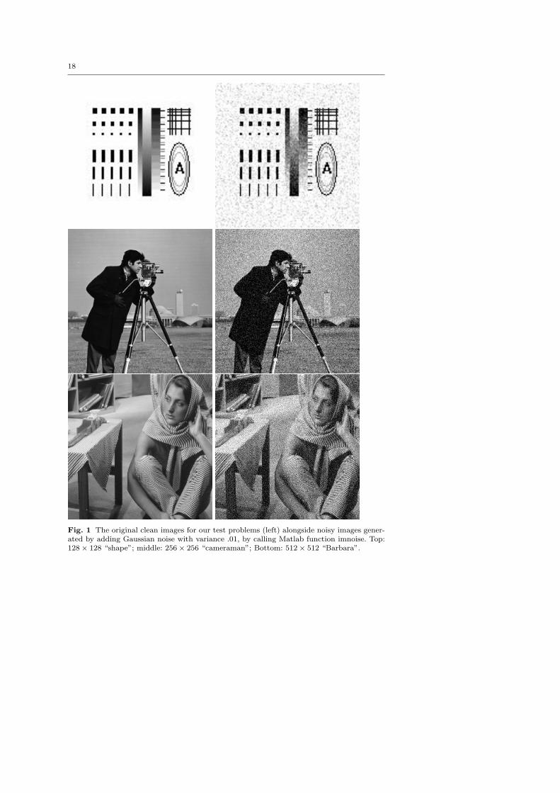
We report on computational experiments for three test problems in imagedenoising. The original clean images and the noisy images used as input tothe denoising codes are shown in Figure 1. The sizes of the discretizations forthe three test problems are 128× 128, 256× 256, and 512× 512, respectively.The noisy images are generated by adding Gaussian noise to the clean imagesusing the MATLAB function imnoise, with variance parameter set to 0.01.The fidelity parameter λ is taken to be 0.045 throughout the experiments.This parameter is inversely related to the noise level σ and usually needs tobe tuned for each individual image to get an optimal visual result.
We tested the following algorithms:
– Chambolle’s semi-implicit gradient descent method [5];– many variants of gradient projection proposed in Section 2;– the SQP method of Section 3;– the CGM method of [8].
We report on a subset of these tests here, including the gradient projectionvariants that gave consistently good results across the three test problems.
In Chambolle’s method, we take the step length to be 0.248 for near-optimal run time, although global convergence is proved in [5] only for steplengths in the range (0, .125). We use the same value αk = 0.248 in AlgorithmGPCL, as in this case it is justified by Theorem 1 and also gives near-optimalrun time.
For all gradient projection variants, we set αmin = 10−5 and αmax = 105.(Performances are insensitive to these choices, as long as αmin is sufficiently
18
Fig. 1 The original clean images for our test problems (left) alongside noisy images gener-ated by adding Gaussian noise with variance .01, by calling Matlab function imnoise. Top:128× 128 “shape”; middle: 256× 256 “cameraman”; Bottom: 512× 512 “Barbara”.
19
small and αmax sufficiently large.) In Algorithm GPLS, we used ρ = 0.5 andµ = 10−4. In Algorithm GPABB, we set γl = 0.1 and γu = 5. In GPBB(safe),we set µ = 10−4 and M = 5 in the formula (22).
We also tried variants of the GPBB methods in which the initial choiceof αk was scaled by a factor of 0.5 at every iteration. We found that thisvariant often enhanced performance. This fact is not too surprising, as wecan see from Section 3 that the curvature of the boundary of constraint set Xsuggests that it is appropriate to add positive diagonal elements to the Hessianapproximation, which corresponds to decreasing the value of αk.
In the CGM implementation, we used a direct solver for the linear systemat each iteration, as the conjugate gradient iterative solver (which is an optionin the CGM code) was slower on these examples. The smooth parameter βis dynamically updated based on duality gap from iteration to iteration. Inparticular, we take β0 = 100 and let βk = βk−1 (Gk/Gk−1)
2, where Gk andGk−1 are the duality gaps for the past two iterations. This simple strategy forupdating β, which is borrowed from interior-point methods, outperforms theclassical CGM approach, producing faster decrease in the duality gap.
All methods are coded in MATLAB and executed on a Dell Precision T5400workstation with 2.66 GHz Inel Quadcore processor and 4GB main memory.It is likely the performance can be improved by recoding the algorithms in Cor C++, but we believe that improvements would be fairly uniform across allthe algorithms.
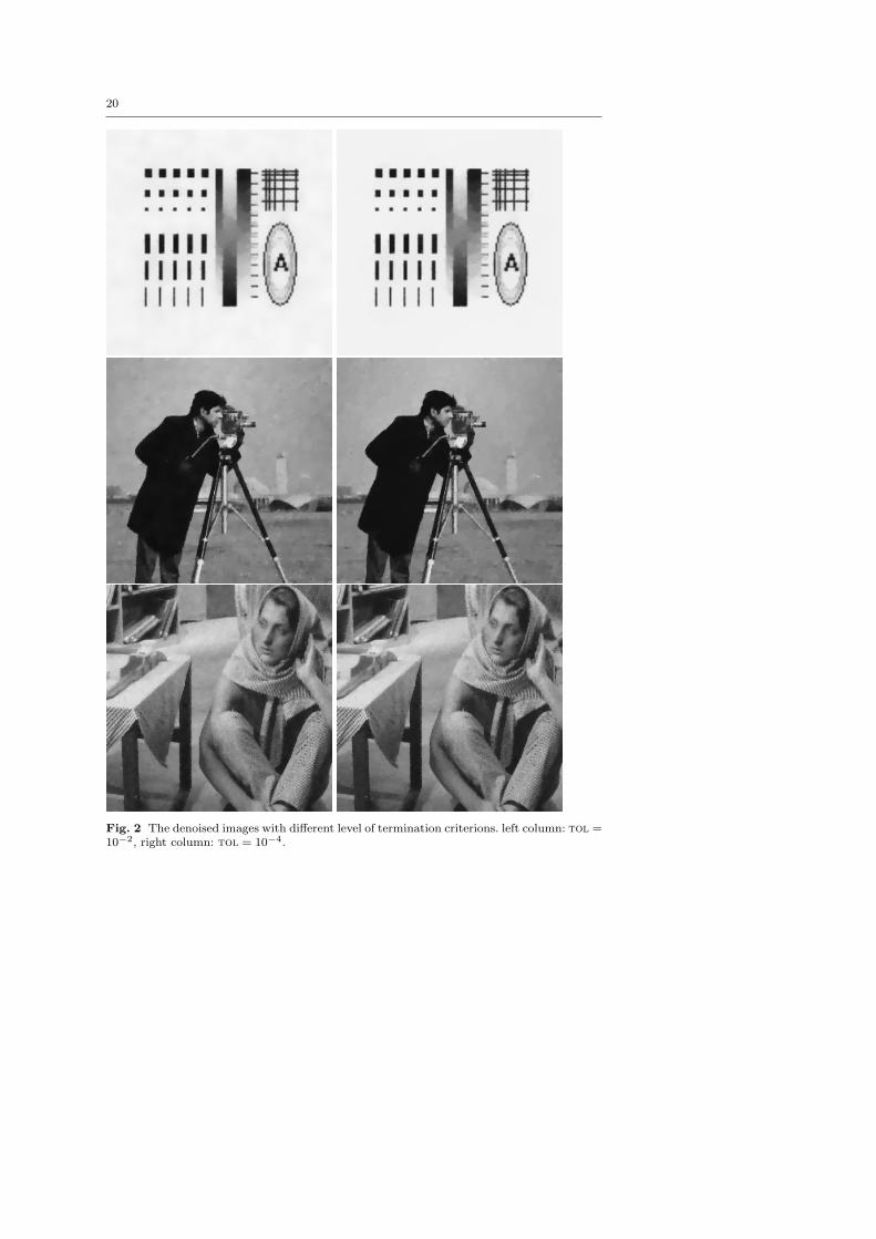
Tables 1, 2, and 3 report number of iterations and average CPU times overten runs, where each run adds a different random noise vector to the trueimage. In all codes, we used the starting point x0 = 0 in each algorithm andthe relative duality gap stopping criterion (31). We vary the threshold tolfrom 10−2 to 10−6, where smaller values of tol yield more accurate solutionsto the optimization formulation.
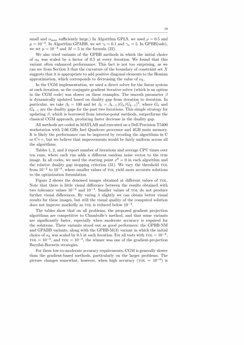
Figure 2 shows the denoised images obtained at different values of tol.Note that there is little visual difference between the results obtained withtwo tolerance values 10−2 and 10−4. Smaller values of tol do not producefurther visual differences. By varing λ slightly we can obtain better visualresults for these images, but still the visual quality of the computed solutiondoes not improve markedly as tol is reduced below 10−2.
The tables show that on all problems, the proposed gradient projectionalgorithms are competitive to Chambolle’s method, and that some variantsare significantly faster, especially when moderate accuracy is required forthe solutions. Three variants stood out as good performers: the GPBB-NMand GPABB variants, along with the GPBB-M(3) variant in which the initialchoice of αk was scaled by 0.5 at each iteration. For all tests with tol = 10−2,tol = 10−3, and tol = 10−4, the winner was one of the gradient-projectionBarzilai-Borwein strategies.
For these low-to-moderate accuracy requirements, CGM is generally slowerthan the gradient-based methods, particularly on the larger problems. Thepicture changes somewhat, however, when high accuracy (tol = 10−6) is
20
Fig. 2 The denoised images with different level of termination criterions. left column: tol =10−2, right column: tol = 10−4.
21
Table 1 Number of iterations and CPU times (in seconds) for problem 1. ∗ = initial αk
scaled by 0.5 at each iteration.
tol = 10−2 tol = 10−3 tol = 10−4 tol = 10−6
Algorithms Iter Time Iter Time Iter Time Iter TimeChambolle 18 0.06 164 0.50 1091 3.34 22975 74.26GPCL 36 0.11 134 0.38 762 2.22 15410 46.34GPLS 22 0.14 166 1.02 891 5.63 17248 113.84GPBB-M 12 0.05 148 0.61 904 3.75 16952 72.82GPBB-M(3) 13 0.05 69 0.28 332 1.32 4065 16.48GPBB-M(3)∗ 11 0.05 47 0.18 188 0.75 2344 9.50GPBB-NM 10 0.04 49 0.18 229 0.85 3865 14.66GPABB 13 0.07 54 0.26 236 1.13 2250 10.90GPBB(safe) 10 0.05 50 0.21 209 0.98 3447 17.32SQPBB-M 11 0.07 48 0.32 170 1.20 3438 25.05CGM 5 1.13 9 2.04 12 2.73 18 4.14
Table 2 Number of iterations and CPU times (in seconds) for problem 2. ∗ = initial αk
scaled by 0.5 at each iteration.
tol = 10−2 tol = 10−3 tol = 10−4 tol = 10−6
Algorithms Iter Time Iter Time Iter Time Iter TimeChambolle 26 0.36 165 2.21 813 11.03 14154 193.08GPCL 32 0.41 116 1.49 535 7.03 9990 132.77GPLS 24 0.55 134 3.84 583 17.48 11070 341.37GPBB-M 20 0.38 124 2.35 576 10.93 10644 203.83GPBB-M(3) 20 0.36 98 1.78 333 6.09 3287 60.44GPBB-M(3)∗ 17 0.31 47 0.86 167 3.05 1698 31.17GPBB-NM 16 0.27 53 0.91 183 3.15 2527 43.80GPABB 16 0.36 47 1.02 158 3.46 1634 35.85GPBB(safe) 16 0.29 52 0.96 170 3.45 2294 51.87SQPBB-M 14 0.37 48 1.36 169 5.16 2537 79.83CGM 5 5.67 9 10.37 13 15.10 19 22.28
required. The rapid asymptotic convergence of CGM is seen to advantage inthis situation, and its runtime improves on all variants of gradient projection.
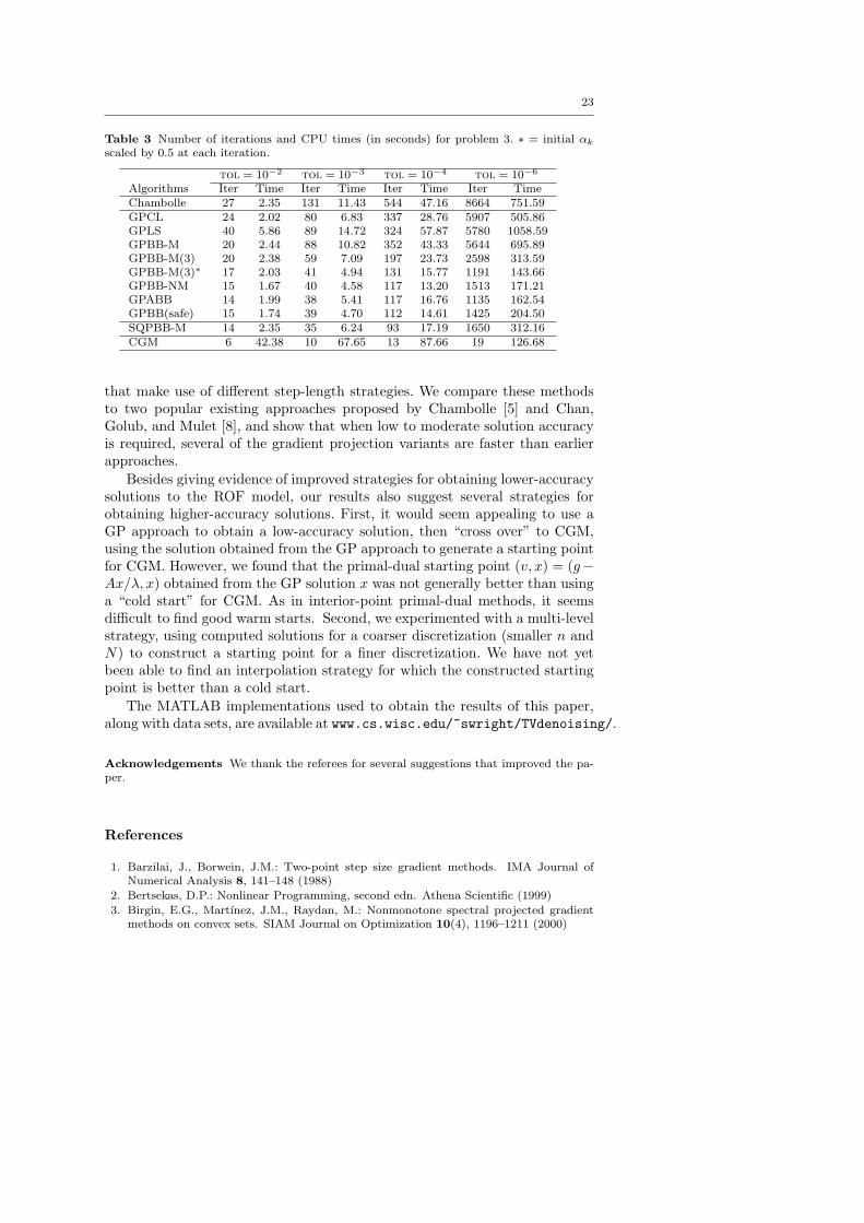
Figure 3 plots the relative duality gap (the left-hand side of (31) againstthe CPU time cost for Chambolle’s method, CGM method, and the GPBB-NM variant of the gradient projection algorithm for each of the three testproblems. Convergence of the “best so far” iterates for GPBB-NM (the lowerbound of this curve) is clearly faster than Chambolle’s method, and also fasterthan CGM until a high-accuracy solution is required.
6 Conclusions and Final Remarks
We have proposed gradient projection algorithms for solving the discretizeddual formulation of the total variation image restoration model of Rudin, Os-her, and Fatemi [17]. The problem has a convex quadratic objective with sep-arable convex constraints, a problem structure that makes gradient projectionschemes practical and simple to implement. We tried different variants of gra-dient projection (including non-monotone Barzilai-Borwein spectral variants)

22
0 5 10 15 20 25 3010−8
10−6
10−4
10−2
100
102
104
106
CPU Time
Rel
ativ
e D
ualit
y G
ap
BB−NMChambolleCGM
0 10 20 30 40 50 60 70 80 9010−8
10−6
10−4
10−2
100
102
104
106
108
CPU Time
Rel
ativ
e D
ualit
y G
ap
BB−NMChambolleCGM
0 50 100 150 200 250 300 35010−8
10−6
10−4
10−2
100
102
104
106
108
CPU Time
Rel
ativ
e D
ualit
y G
ap
BB−NMChambolleCGM
Fig. 3 Duality gap vs. CPU time for GPBB-NM, Chambolle, and CGT codes, for problemsProlems 1, 2, and 3, respectively.
23
Table 3 Number of iterations and CPU times (in seconds) for problem 3. ∗ = initial αk
scaled by 0.5 at each iteration.
tol = 10−2 tol = 10−3 tol = 10−4 tol = 10−6
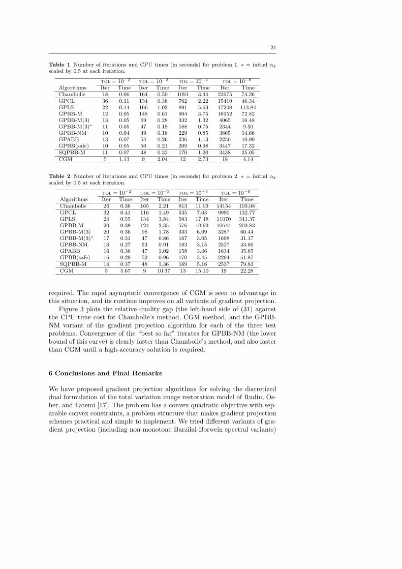
Algorithms Iter Time Iter Time Iter Time Iter TimeChambolle 27 2.35 131 11.43 544 47.16 8664 751.59GPCL 24 2.02 80 6.83 337 28.76 5907 505.86GPLS 40 5.86 89 14.72 324 57.87 5780 1058.59GPBB-M 20 2.44 88 10.82 352 43.33 5644 695.89GPBB-M(3) 20 2.38 59 7.09 197 23.73 2598 313.59GPBB-M(3)∗ 17 2.03 41 4.94 131 15.77 1191 143.66GPBB-NM 15 1.67 40 4.58 117 13.20 1513 171.21GPABB 14 1.99 38 5.41 117 16.76 1135 162.54GPBB(safe) 15 1.74 39 4.70 112 14.61 1425 204.50SQPBB-M 14 2.35 35 6.24 93 17.19 1650 312.16CGM 6 42.38 10 67.65 13 87.66 19 126.68
that make use of different step-length strategies. We compare these methodsto two popular existing approaches proposed by Chambolle [5] and Chan,Golub, and Mulet [8], and show that when low to moderate solution accuracyis required, several of the gradient projection variants are faster than earlierapproaches.
Besides giving evidence of improved strategies for obtaining lower-accuracysolutions to the ROF model, our results also suggest several strategies forobtaining higher-accuracy solutions. First, it would seem appealing to use aGP approach to obtain a low-accuracy solution, then “cross over” to CGM,using the solution obtained from the GP approach to generate a starting pointfor CGM. However, we found that the primal-dual starting point (v, x) = (g−Ax/λ, x) obtained from the GP solution x was not generally better than usinga “cold start” for CGM. As in interior-point primal-dual methods, it seemsdifficult to find good warm starts. Second, we experimented with a multi-levelstrategy, using computed solutions for a coarser discretization (smaller n andN) to construct a starting point for a finer discretization. We have not yetbeen able to find an interpolation strategy for which the constructed startingpoint is better than a cold start.
The MATLAB implementations used to obtain the results of this paper,along with data sets, are available at www.cs.wisc.edu/~swright/TVdenoising/.
Acknowledgements We thank the referees for several suggestions that improved the pa-per.
References
1. Barzilai, J., Borwein, J.M.: Two-point step size gradient methods. IMA Journal ofNumerical Analysis 8, 141–148 (1988)
2. Bertsekas, D.P.: Nonlinear Programming, second edn. Athena Scientific (1999)
3. Birgin, E.G., Martınez, J.M., Raydan, M.: Nonmonotone spectral projected gradientmethods on convex sets. SIAM Journal on Optimization 10(4), 1196–1211 (2000)

24
4. Carter, J.L.: Dual method for total variation-based image restoration. Report 02-13,UCLA CAM (2002)
5. Chambolle, A.: An algorithm for total variation minimization and applications. Journalof Mathematical Imaging and Visualization 20, 89–97 (2004)
6. Chambolle, A., Lions, P.L.: Image recovery via total variation minimization and relatedproblmes. Numerische Mathematik 76, 167–188 (1997)
7. Chan, T.F., Esedoglu, S., Park, F., Yip, A.: Total variation image restoration: Overviewand recent developments. In: N. Paragios, Y. Chen, O. Faugeras (eds.) Handbook ofMathematical Models in Computer Vision. Springer (2005)
8. Chan, T.F., Golub, G.H., Mulet, P.: A nonlinear primal-dual method for total variationbased image restoration. SIAM Journal of Scientific Computing 20, 1964–1977 (1999)
9. Chan, T.F., Zhu, M.: Fast algorithms for total variation-based image processing. In:Proceedings of the 4th ICCM. Hangzhuo, China (2007)
10. Dai, Y.H., Fletcher, R.: Projected barzilai-borwein methods for large-scale box-constrained quadratic programming. Numerische Mathematik 100, 21–47 (2005)
11. Dai, Y.H., Hager, W.W., Schittkowski, K., Zhang, H.: The cyclic Barzilai-Borweinmethod for unconstrained optimization. IMA Journal of Numerical Analysis 26, 604–627 (2006)
12. Ekeland, I., Temam: Convex Analysis and Variational Problems. SIAM Classics inApplied Mathematics. SIAM (1999)
13. Goldfarb, D., Yin, W.: Second-order cone programming methods for total variation-based image restoration. SIAM Journal on Scientific Computing 27, 622–645 (2005)
14. Hintermuller, M., Stadler, G.: An infeasible primal-dual algorithm for TV-based inf-convolution-type image restoration. SIAM Journal on Scientific Computing 28, 1–23(2006)
15. Hiriart-Urruty, J., Lemarechal, C.: Convex Analysis and Minimization Algorithms,vol. I. Springer-Verlag, Berlin (1993)
16. Osher, S., Marquina, A.: Explicit algorithms for a new time dependent model based onlevel set motion for nonlinear deblurring and noise removal. SIAM Journal of ScientificComputing 22, 387–405 (2000)
17. Rudin, L., Osher, S., Fatemi, E.: Nonlinear total variation based noise removal algo-rithms. Physica D 60, 259–268 (1992)
18. Serafini, T., Zanghirati, G., Zanni, L.: Gradient projection methods for large quadraticprograms and applications in training support vector machines. Optimization Methodsand Software 20(2–3), 353–378 (2004)
19. Vogel, C.R., Oman, M.E.: Iterative methods for total variation denoising. SIAM Journalof Scientific Computing 17, 227–238 (1996)
20. Wang, Y., Ma, S.: Projected barzilai-borwein methods for large-scale nonnegative imagerestoration. Inverse Problems in Science and Engineering 15(6), 559–583 (2007)