duality theory - international university of japan€¦ · section 6.5 focuses on the role of...
TRANSCRIPT

~
~rive M and v for this
~tion, another option is ~ich is the preliminary C H E R l of the nonzero coeffi~nd X7. Repeat part (b) r you derive the new v, ne final row 0 for this ~ (b) . ~ CPF solution corre~ in the final simplex
Duality Theory
One of the most important discoveries in the early development of linear programming ~es in the optimal solu.; was the concept of duality and its many important ramifications. This discovery re
vealed that every linear programming problem has associated with it another linear pro~ the given information
gramming problem called the dual. The relationships between the dual problem and the r Gaussian elimination.
original problem (called the primal) prove to be extremely useful in a variety of ways.i shadow prices. For example, you soon will see that the shadow prices described in Sec. 4.7 actually are le defining equations of provided by the optimal solution for the dual problem. We shall describe many other valu~lve these equations to able applications of duality theory in this chapter as well.
optimal BF solution, For greater clarity, the first three sections discuss duality theory under the asB- 1
f to solve for the ' sumption that the primal linear programming problem is in our standard form (but with es y*. Then apply the no restriction that the bi values need to be positive). Other forms are then discussed in ithe simplex method to Sec. 6.4. We begin the chapter by introducing the essence of duality theory and its ap
plications. We then describe the economic interpretation of the dual problem (Sec. 6.2) fundamental insight pre and delve deeper into the relationships between the primal and dual problems (Sec. 6.3). ~te final simplex tableau.
Section 6.5 focuses on the role of duality theory in sensitivity analysis. (As discussed in detail in the next chapter, sensitivity analysis involves the analysis of the effect on ~-2. Let X6 and X7 be the
lraints, respectively. You the optimal solution if changes occur in the values of some of the parameters of the ng basic variable and X7 model.) teration of the simplex iable and X6 is the leavltion. Use the procedure one iteration to the next fier the second iteration.
method step by step to
method step by step to
method step by step to
THE ESSENCE OF DUALITY THEORY
Given our standard form for the primal problem at the left (perhaps after conversion from another form), its dual problem has the form shown to the right.
197

198 CHAPTER 6 DUALITY THEORY
Primal Problem Dual Problem
n m
Maximize Z = I c)x), Minimize W= I biYi, ) = 1 i=1
subject to subject to
n m
I aijx)::; bi , for i = I, 2, ... , m I aijYi ~ c), for j = 1, 2, ... , n )=1 i = 1
and and
for j = I, 2, ... , n. Yi ~ 0, for i = 1, 2, ... , m.
Thus, with the primal problem in maximization form, the dual problem is in m' . . form instead. Furthermore, the dual problem uses exactly the same parameters as the mal problem, but in different locations, as summarized below.
1. The coefficients in the objective function of the primal problem are the right-hand of the functional constraints in the dual problem.
2. The right-hand sides of the functional constraints in the primal problem are the ficients in the objective function of the dual problem.
3. The coefficients of a variable in the functional constraints of the primal problem the coefficients in a functional constraint of the dual problem.
To highlight the comparison, now look at these same two problems in matrix notation (as introduced at the beginning of Sec. 5.2), where c and y = [yJ, Y2, ... , Ym] are row vectors but b and x are column vectors.
Primal Proble}n
Maximize Z= ex,
subject to
Ax::; b
and
x ~ O.
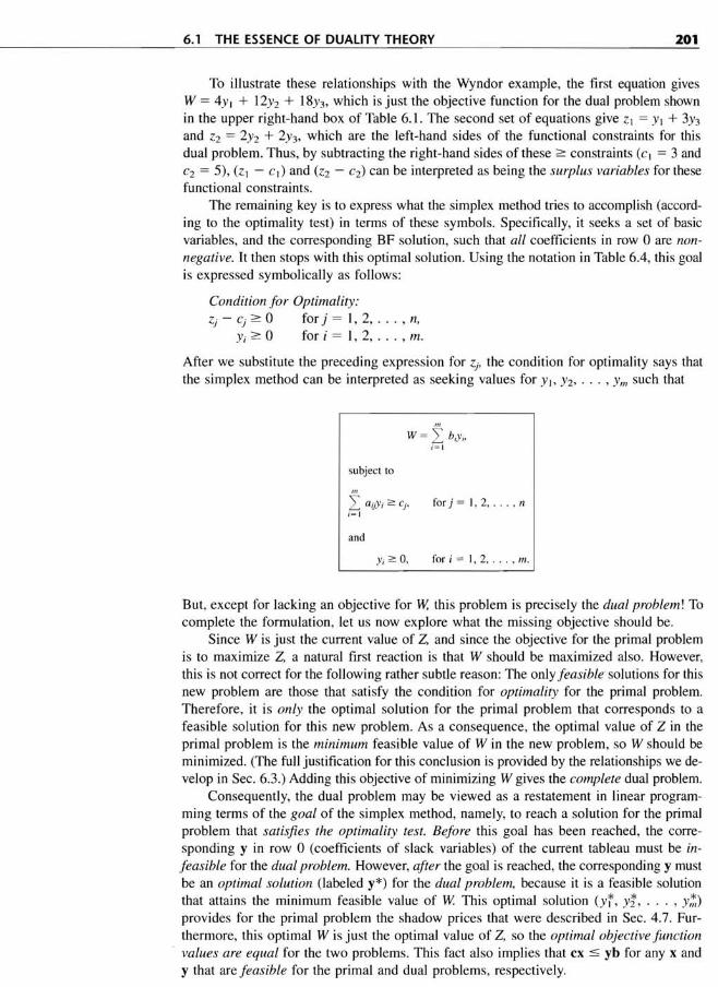
To illustrate, the primal and dual problems for the Wyndor Glass Co. example of Sec. 3.1 are shown in Table 6.1 in both algebraic and matrix form.
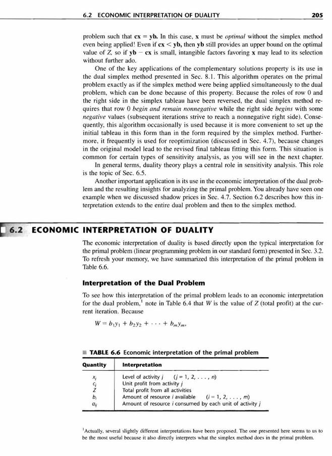
The primal-dual table for linear programming (Table 6.2) also helps to highlight the correspondence between the two problems. It shows all the linear programming parameters (the au, hi> and c) and how they are used to construct the two problems. All the headings for the primal problem are horizontal, whereas the headings for the dual problem are read by turning the book sideways. For the primal problem, each column (except the right-side column) gives the coefficients of a single variable in the respective constraints and then in the objective function, whereas each row (except the bottom one) gives the parameters for a single contraint. For the dual problem, each row (except the right-side row) gives the coefficients of a single variable in the respective constraints and then in the objective function, whereas each column (except the rightmost one) gives the parameters for a single constraint. In addition, the right-side column gives the right-hand sides for the primal problem and the objective function coefficients for the dual problem,
Dual Problem
Minimize W=yb,
subject to
yA ~e
and
y~O.

i = 1,2, . . . ,n
1= 1,2, ... , m.
m is in minimization r.lrameters as the pri-
I the right-hand sides
roblem are the coef
primal problem are
I
~ matrix notation (as !. , Ym] are row vec
example of Sec. 3.1
o helps to highlight ~ programming pa~o problems. All the ~s for the dual probtl, each column (ex~le in the respective ~ept the bottom one) ach row (except the ~tive constraints and ~m6st one) gives the 'gives the right-hand or the dual problem,
6.1 THE ESSENCE OF DUALITY THEORY
• TABLE 6.1 Primal and dual problems for the Wyndor Glass Co. example Primal Problem
in Algebraic Form
Maximize
subject to
and
::; 4
2X2 ::; 12
3x, + 2X2 ::; 18
Primal Problem in Matrix Form
Maximize
subject to
and
Minimize
subject to
and
Dual Problem in Algebraic Form
+ 3Y3;::: 3
Y2;::: 0,
Dual Problem in Matrix Form
Minimize W ~ [Yl, y" Ydr ~~] subject to
[Yl, Y" Y3J r~ ~]" [3, 5J
and
199
• TABLE 6.2 Primal-dual table for linear programming, illustrated by the Wyndor Glass Co. example
(a) General Case
., c CII ~ .._'100 :t 0
CII o v
Yl Y2
Ym
(b) Wyndor Glass Co. Example
Xl X2
Y, 1 0 ::; 4
Y2 0 '2 ::; 12
Y3 3 2 ::; 18
VI VI 3 5
Xl
VI
Primal Problem
Coefficient of:
X2
VI
Coefficients for Objective Function
Maximize
VI
Right Side

200 CHAPTER 6 DUALITY THEORY
whereas the bottom row gives the objective function coefficients for the primal and the right-hand sides for the dual problem.
Consequently, we now have the following general relationships between the and dual problems.
1. The parameters for a (functional) constraint in either problem are the coefficients variable in the other problem.
2. The coefficients in the objective function of either problem are the right-hand s" the other problem.
Thus, there is a direct correspondence between these entities in the two problems, as marized in Table 6.3. These correspondences are a key to some of the applications of ality theory, including sensitivity analysis.
The Solved Examples section of the book's website provides another example ing the primal-dual table to construct the dual problem for a linear programming
Origin of the Dual Problem
Duality theory is based directly on the fundamental insight (particularly with row 0) presented in Sec. 5.3. To see why, we continue to use the notation intn)dll(;ed Table 5.9 for row 0 of the final tableau, except for replacing Z* by W* and dropping asterisks from z* and y* when referring to any tableau. Thus, at any given iteration simplex method for the primal problem, the current numbers in row 0 are shown in the (partial) tableau given in Table 6.4. For the coefficients of x(, Xz, ... ,
recall that z = (z" Zz, ... , Zn) denotes the vector that the simplex method added to vector of initial coefficients, -C, in the process of reaching the current tableau. (Do confuse z with the value of the objective function 20) Similarly, since the initial cients of Xn + (, Xn+Z, ... , Xn + m in row 0 all are 0, y = (y" Yz, ... , Ym) denotes the tor that the simplex method has added to these coefficients. Also recall [see Eq. (1) in statement of the fundamental insight in Sec. 5.3] that the fundamental insight led to following relationships between these quantities and the parameters of the original
m
W = yb = I biYi, i = \
z = yA, so Zj = Im
aijYi, for j = 1, 2, . .. , n. i=\
TABLE 6.3 Correspondence between entities in primal and dual problems
One Problem Other Problem
Constraint i ~ Variable i Objective function ( ) Right-hand sides
• TABLE 6.4 Notation for entries in row 0 of a simplex tableau
Iteration
Any
Basic Variable
z
Eq.
(0)
Coefficient of:
Xn + l Xn+2
i
201 6.1 THE ESSENCE OF DUALITY THEORY
the primal problem
between the primal
the coefficients of a
right-hand sides for
o problems, as sum~ applications of du
ther example of uslrogramming model.
.larly with regard to Itatian introduced in V* and dropping the ~iven iteration of the w 0 are denoted as s of X), X2, ..• , Xn>
nethod added to the ent tableau. (Do not ce the initial coeffiYm) denotes the vecn[see Eq. (1) in the tal insight led to the rthe original model:
------i Right Xn+ m Side
Ym W
To illustrate these relationships with the Wyndor example, the first equation gives W = 4YI + 12Y2 + 18Y3, which is just the objective function for the dual problem shown in the upper right-hand box of Table 6.1. The second set of equations give ZI = YI + 3Y3 and Z2 = 2Y2 + 2Y3, which are the left-hand sides of the functional constraints for this dual problem. Thus, by subtracting the right-hand sides of these ~ constraints (CI = 3 and C2 = 5), (z\ - CI) and (Z2 - C2) can be interpreted as being the surplus variables for these functional constraints.
The remaining key is to express what the simplex method tries to accomplish (according to the optimality test) in terms of these symbols. Specifically, it seeks a set of basic variables, and the corresponding BF solution, such that all coefficients in row 0 are nonnegative. It then stops with this optimal solution. Using the notation in Table 6.4, this goal is expressed symbolically as follows:
Condition for Optimality: Zj - Cj ~ 0 for j = 1, 2, . . . , n,
Yi ~ 0 for i = I, 2, ... , m.
After we substitute the preceding expression for Zj' the condition for optimality says that the simplex method can be interpreted as seeking values for Y), Y2, ... , Ym such that
W= Im
biYi, i=l
subject to
I m
aUYi ~ Cj, for j = 1, 2, ... , n i=j
and
for i = 1, 2, ... , m.
But, except for lacking an objective for W, this problem is precisely the dual problem! To complete the formulation, let us now explore what the missing objective should be.
Since W is just the current value of Z, and since the objective for the primal problem is to maximize Z, a natural first reaction is that W should be maximized also. However, this is not correct for the following rather subtle reason: The only feasible solutions for this new problem are those that satisfy the condition for optimality for the primal problem. Therefore, it is only the optimal solution for the primal problem that corresponds to a feasible solution for this new problem. As a consequence, the optimal value of Z in the primal problem is the minimum feasible value of W in the new problem, so W should be minimized. (The full justification for this conclusion is provided by the relationships we develop in Sec. 6.3.) Adding this objective of minimizing W gives the complete dual problem.
Consequently, the dual problem may be viewed as a restatement in linear programming terms of the goal of the simplex method, namely, to reach a solution for the primal problem that satisfies the optimality test. Before this goal has been reached, the corresponding y in row 0 (coefficients of slack variables) of the current tableau must be infeasible for the dual problem. However, after the goal is reached, the corresponding y must be an optimal solution (labeled y*) for the dual problem, because it is a feasible solution that attains the minimum feasible value of W This optimal solution (yi, yi, ... , Y!) provides for the primal problem the shadow prices that were described in Sec. 4.7. Furthermore, this optimal W is just the optimal value of Z, so the optimal objective function values are equal for the two problems. This fact also implies that ex ~ yb for any x and y that are feasible for the primal and dual problems, respectively.

202 CHAPTER 6 DUALITY THEORY
To illustrate, the left-hand side of Table 6.5 shows row °for the respective· tions when the simplex method is applied to the Wyndor Glass Co. example. In case, row °is partitioned into three parts: the coefficients of the decision variables (x" the coefficients of the slack variables (X3, X4, xs), and the right-hand side (value of Z). the coefficients of the slack variables give the corresponding values of the dual (Yl' Yb Y3), each row °identifies a corresponding solution for the dual problem, as in the y" Y2, and Y3 columns of Table 6.5. To interpret the next two columns, recall (z, - c,) and (Z2 - C2) are the surplus variables for the functional constraints in the problem, so the full dual problem after augmenting with these surplus variables is
Minimize
subject to
y, + 3Y3 - (z, - c,) = 3 2Y2 + 2Y3 - (Z2 - C2) = 5
and
YI 2:: 0, Y2 2:: 0, Y3 2:: 0.
Therefore, by using the numbers in the y" Yb and Y3 columns, the values of these variables can be calculated as
z, - c, = YI + 3Y3 - 3, Z2 - C2 = 2Y2 + 2Y3 - 5.
Thus, a negative value for either surplus variable indicates that the corresponding straint is violated. Also included in the rightmost column of the table is the caU';UlaLai value of the dual objective function W = 4y, + 12Y2 + 18Y3.
As displayed in Table 6.4, all these quantities to the right of row °in Table 6.5 al· ready are identified by row °without requiring any new calculations. In particular, in Table 6.5 how each number obtained for the dual problem already appears in row 0 the spot indicated by Table 6.4.
For the initial row 0, Table 6.5 shows that the corresponding dual (y" Y2, Y3) = (0, 0, 0) is infeasible because both surplus variables are negative. The first eration succeeds in eliminating one of these negative values, but not the other. After two erations, the optimality test is satisfied for the primal problem because all the dual and surplus variables are nonnegative. This dual solution (Yr, yi, yj) = (0, i, 1) is (as could be verified by applying the simplex method directly to the dual problem), so optimal value of Z and W is Z* = 36 = W* .
• TABLE 6.5 Row 0 and corresponding dual solution for each iteration for the Wyndor Glass Co. example
Iteration
0
2
Primal Problem
[-3, -5
[-3, 0
[ 0, 0
Row 0
0,
0,
0, 5 2'
0
0
0, 3 2'
Dual Problem
Yl Y2 Y3 Zl - Cl
0]
30]
0
0
0 5 2
0
0
-3
-3
-5
0
36] 0 3 2 0 0

!
I
203 6.1 THE ESSENCE OF DUALITY THEORY
the respective iterao. example. In each Ion variables (x I, X2), Ie (value of Z). Since of the dual variables I problem, as shown columns, recall that mstraints in the dual )lus variables is
lues of these surplus
corresponding con)le is the calculated
w0 in Table 6.5 al~ . In particular, note appears in row °in
lding dual solution ~egative. The first ite other. After two itall the dual variables ;: (0, ~, 1) is optimal ual problem), so the
3 -5 0
3 0 30
o 0 36
Summary of Primal-Dual Relationships
Now let us summarize the newly discovered key relationships between the primal and dual problems.
Weak duality property: If x is a feasible solution for the primal problem and y is a feasible solution for the dual problem, then
ex ::; yb.
For example, for the Wyndor Glass Co. problem, one feasible solution is XI = 3, X2 = 3, which yields Z = ex = 24, and one feasible solution for the dual problem is YI = 1, Yz = 1, Y3 = 2, which yields a larger objective function value W = yb = 52. These are just sample feasible solutions for the two problems. For any such pair of feasible solutions, this inequality must hold because the maximum feasible value of Z = ex (36) equals the minimum feasible value of the dual objective function W = yb, which is our next property.
Strong duality property: If x* is an optimal solution for the primal problem and y* is an optimal solution for the dual problem, then
cx* = y*b.
Thus, these two properties imply that ex < yb for feasible solutions if one or both of them are not optimal for their respective problems, whereas equality holds when both are optimal.
The weak duality property describes the relationship between any pair of solutions for the primal and dual problems where both solutions are feasible for their respective problems. At each iteration, the simplex method finds a specific pair of solutions for the two problems, where the primal solution is feasible but the dual solution is not feasible (except at the final iteration). Our next property describes this situation and the relationship between this pair of solutions.
Complementary solutions property: At each iteration, the simplex method simultaneously identifies a CPF solution x for the primal problem and a complementary solution y for the dual problem (found in row 0, the coefficients of the slack variables), where
ex = yb.
If x is not optimal for the primal problem, then y is not feasible for the dual problem.
To illustrate, after one iteration for the Wyndor Glass Co. problem, XI = 0, Xz = 6, and YI = 0, Y2 = %, Y3 = 0, with ex = 30 = yb. This x is feasible for the primal problem, but this y is not feasible for the dual problem (since it violates the constraint, YI + 3Y3 ~ 3).
The complementary solutions property also holds at the final iteration of the simplex method, where an optimal solution is found for the primal problem. However, more can be said about the complementary solution y in this case, as presented in the next property.
Complementary optimal solutions property: At the final iteration, the simplex method simultaneously identifies an optimal solution x* for the primal problem and a complementary optimal solution y* for the dual problem (found in row 0, the coefficients of the slack variables), where
cx* = y*b.
The Yf are the shadow prices for the primal problem.
For the example, the final iteration yields xi = 2, xi = 6, and yi = 0, yi = ~, yj = 1, with cx* = 36 = y*b.

204 CHAPTER 6 DUALITY THEORY
We shall take a closer look at some of these properties in Sec. 6.3. There you will see that the complementary solutions property can be extended considerably further. In partic· ular, after slack and surplus variables are introduced to augment the respective problems, every basic solution in the primal problem has a complementary basic solution in the dual problem. We already have noted that the simplex method identifies the values of the sur· plus variables for the dual problem as Zj - Cj in Table 6.4. This result then leads to an ad· ditional complementary slackness property that relates the basic variables in one problem to the nonbasic variables in the other (Tables 6.7 and 6.8), but more about that later.
In Sec. 6.4, after describing how to construct the dual problem when the primal prob· lem is not in our standard form, we discuss another very useful property, which is summarized as follows:
Symmetry property: For any primal problem and its dual problem, all relationships between them must be symmetric because the dual of this dual problem is this primal problem.
Therefore, all the preceding properties hold regardless of which of the two problems is labeled as the primal problem. (The direction of the inequality for the weak duality property does require that the primal problem be expressed or reexpressed in maximization form and the dual problem in minimization form.) Consequently, the simplex method can be applied to either problem, and it simultaneously will identify complementary solutions (ultimately a complementary optimal solution) for the other problem.
So far, we have focused on the relationships between feasible or optimal solutions in the primal problem and corresponding solutions in the dual problem. However, it is possible that the primal (or dual) problem either has no feasible solutions or has feasible solutions but no optimal solution (because the objective function is unbounded). Our final ECON property summarizes the primal-dual relationships under all these possibilities.
Duality theorem: The following are the only possible relationships between the primal and dual problems.
1. If one problem has feasible solutions and a bounded objective function (and so has an optimal solution), then so does the other problem, so both the weak and strong duality properties are applicable.
2. If one problem has feasible solutions and an unbounded objective function (and so no optimal solution), then the other problem has no feasible solutions.
3. If one problem has no feasible solutions, then the other problem has either no feasible solutions or an unbounded objective function.
Applications
As we have just implied, one important application of duality theory is that the dual problem can be solved directly by the simplex method in order to identify an optimal solution for the primal problem. We discussed in Sec. 4.8 that the number of functional constraints affects the computational effort of the simplex method far more than the number of variables does. If m > n, so that the dual problem has fewer functional constraints (n) than the primal problem (m), then applying the simplex method directly to the dual problem instead of the primal problem probably will achieve a substantial reduction in computational effort.
The weak and strong duality properties describe key relationships between the primal and dual problems. One useful application is for evaluating a proposed solution for the primal problem. For example, suppose that x is a feasible solution that has been proposed for implementation and that a feasible solution y has been found by inspection for the dual
205 6.2 ECONOMIC INTERPRETATION OF DUALITY
~. There you will see Jly further. In particrespective problems, : solution in the dual ~e values of the surthen leads to an ad-
Ibles in one problem tbout that later. hen the primal probJerty, which is sum-
em, all relationdual problem is
the two problems is ~ weak duality propied in maximization simplex method can )lementary solutions
optimal solutions in , However, it is poss or has feasible so
problem such that ex = yb. In this case, x must be optimal without the simplex method even being applied! Even if ex < yb, then yb still provides an upper bound on the optimal value of Z, so if yb - ex is small, intangible factors favoring x may lead to its selection without further ado.
One of the key applications of the complementary solutions property is its use in the dual simplex method presented in Sec. 8.1. This algorithm operates on the primal problem exactly as if the simplex method were being applied simultaneously to the dual problem, which can be done because of this property. Because the roles of row 0 and the right side in the simplex tableau have been reversed, the dual simplex method requires that row 0 begin and remain nonnegative while the right side begins with some negative values (subsequent iterations strive to reach a nonnegative right side). Consequently, this algorithm occasionally is used because it is more convenient to set up the initial tableau in this form than in the form required by the simplex method. Furthermore, it frequently is used for reoptimization (discussed in Sec. 4.7), because changes in the original model lead to the revised final tableau fitting this form. This situation is common for certain types of sensitivity analysis, as you will see in the next chapter.
In general terms, duality theory plays a central role in sensitivity analysis. This role is the topic of Sec. 6.5.
Another important application is its use in the economic interpretation of the dual problem and the resulting insights for analyzing the primal problem. You already have seen one example when we discussed shadow prices in Sec. 4.7. Section 6.2 describes how this interpretation extends to the entire dual problem and then to the simplex method.
,bounded). Our final 1 . ECONOMIC INTERPRETATION OF DUALITY
Issibilities. The economic interpretation of duality is based directly upon the typical interpretation for
ips between the the primal problem (linear programming problem in our standard form) presented in Sec. 3.2. To refresh your memory, we have summarized this interpretation of the primal problem in
e function (and Table 6.6.
) both the weak Interpretation of the Dual Problem
jective function To see how this interpretation of the primal problem leads to an economic interpretation lsible solutions. for the dual problem, I note in Table 6.4 that W is the value of Z (total profit) at the curm has either no rent iteration. Because
i that the dual prob• TABLE 6.6 Economic interpretation of the primal problem
an optimal solution mctional constraints Quantity
the number of variconstraints (n) than :0 the dual problem luction in computa
between the primal solution for the, pri
Interpretation
Level of activity j (j = 1, 2, ... , n) Unit profit from activity j Total profit from all activities Amount of resource i available (i = 1, 2, ... , m) Amount of resource i consumed by each unit of activity j
s been proposed for I Actually, several slightly different interpretations have been proposed. The one presented here seems to us to JeCtion for the dual be the most useful because it also directly interprets what the simplex method does in the primal problem.
206 CHAPTER 6 DUALITY THEORY
each biYi can thereby be interpreted as the current contribution to profit by having bi units of resource i available for the primal problem. Thus,
The dual variable Yi is interpreted as the contribution to profit per unit of resource i (i = 1, 2, ... , m), when the current set of basic variables is used to obtain the primal solution.
In other words, the Yi values (or l values in the optimal solution) are just the shadow prices discussed in Sec. 4.7.
For example, when iteration 2 of the simplex method finds the optimal solution for the Wyndor problem, it also finds the optimal values of the dual variables (as shown in the bottom row of Table 6.5) to be yi = 0, yi = ~, and yj = 1. These are precisely the shadow prices found in Sec. 4.7 for this problem through graphical analysis. Recall that the resources for the Wyndor problem are the production capacities of the three plants being made available to the two new products under consideration, so that bi is the number of hours of production time per week being made available in Plant i for these new products, where i = 1,2, 3. As discussed in Sec. 4.7, the shadow prices indicate that individually increasing any bi by 1 would increase the optimal value of the objective function (total weekly profit in units of thousands of dollars) by y'j. Thus, yi can be interpreted as the contribution to profit per unit of resource i when using the optimal solution.
This interpretation of the dual variables leads to our interpretation of the overall dual problem. Specifically, since each unit of activity j in the primal problem consumes aij
units of resource i,
~~ I aijYi is interpreted as the current contribution to profit of the mix of resources that would be consumed if 1 unit of activity j were used (j = 1,2, ... , n).
For the Wyndor problem, 1 unit of activity j corresponds to producing 1 batch of product j per week, where j = 1, 2. The mix of resources consumed by producing 1 batch of product 1 is 1 hour of production time in Plant 1 and 3 hours in Plant 3. The corresponding mix per batch of product 2 is 2 hours each in Plants 2 and 3. Thus, YI + 3Y3 and 2Y2 + 2Y3 are interpreted as the current contributions to profit (in thousands of dollars per week) of these respective mixes of resources per batch produced per week of the respective products.
For each activity j, this same mix of resources (and more) probably can be used in other ways as well, but no alternative use should be considered if it is less profitable than I unit of activity j. Since Cj is interpreted as the unit profit from activity j, each functional constraint in the dual problem is interpreted as follows:
~r= I aijYi::2: Cj says that the actual contribution to profit of the above mix of resources must be at least as much as if they were used by 1 unit of activity j; otherwise, we would not be making the best possible use of these resources.
For the Wyndor problem, the unit profits (in thousands of dollars per week) are CI = 3 and C2 = 5, so the dual functional constraints with this interpretation are YI + 3Y3 2: 3 and 2Y2 + 2Y3 ::2: 5. Similarly, the interpretation of the nonnegativity constraints is the following:
Yi ::2: °says that the contribution to profit of resource i (i = I, 2, ... , m) must be nonnegative: otherwise, it would be better not to use this resource at all.
The objective
Minimize W= Im
biYi i=1

i
207 6.2 ECONOMIC INTERPRETATION OF DUALITY
'Oftt by having bi units
r unit of resource [sed to obtain the
I are just the shadow
~ optimal solution for ariables (as shown in lese are precisely the . analysis. Recall that ~s of the three plants so that bi is the numin Plant i for these
adow prices indicate nal value of the oblars) by y;. Thus, Y; rce i when using the
on of the overall dual roblem consumes aij
.mix of resources 12, ... ,n).
19 1 batch of product Icing 1 batch of prod3. The corresponding + 3Y3 and 2Y2 + 2Y3
:dollars per week) of e respective products. bably can be used in ls less profitable than rity j, each functional
lbove mix of re)f activity j; othresources.
,er week) are CI = 3 .on are YI + 3Y3 2 3 Ity constraints is the
~, ... , m) must purce at all.
can be viewed as minimizing the total implicit value of the resources consumed by the activities. For the Wyndor problem, the total implicit value (in thousands of dollars per week) of the resources consumed by the two products is W = 4Yl + 12Y2 + 18Y3'
This interpretation can be sharpened somewhat by differentiating between basic and nonbasic variables in the primal problem for any given BF solution (x], X2, ... , xn+m)' Recall that the basic variables (the only variables whose values can be nonzero) always have a coefficient of zero in row O. Therefore, referring again to Table 6.4 and the accompanying equation for Zj' we see that
m
I aijYi = Cj' if Xj > 0 (j = 1, 2, ... , n), i=1
Yi = 0, if Xn+i > 0 (i = 1, 2, ... , m).
(This is one version of the complementary slackness property discussed in Sec. 6.3.) The economic interpretation of the first statement is that whenever an activity j operates at a strictly positive level (x) > 0), the marginal value of the resources it consumes must equal (as opposed to exceeding) the unit profit from this activity. The second statement implies that the marginal value of resource i is zero (Yi = 0) whenever the supply of this resource is not exhausted by the activities (Xn+i > 0). In economic terminology, such a resource is a "free good"; the price of goods that are oversupplied must drop to zero by the law of supply and demand. This fact is what justifies interpreting the objective for the dual problem as minimizing the total implicit value of the resources consumed, rather than the resources allocated.
To illustrate these two statements, consider the optimal BF solution (2, 6, 2, 0, 0) for the Wyndor problem. The basic variables are Xl> X2, and X3, so their coefficients in row 0 are zero, as shown in the bottom row of Table 6.5. This bottom row also gives the corresponding dual solution: yi = 0, yi = ~,yj = 1, with surplus variables (zi - c,) = 0 and (zi - C2) = O. Since XI > 0 and X2 > 0, both these surplus variables and direct calculations indicate that yi + 3yj = CI = 3 and 2yi + 2yj = C2 = 5. Therefore, the value of the resources consumed per batch of the respective products produced does indeed equal the respective unit profits. The slack variable for the constraint on the amount of Plant I capacity used is X3 > 0, so the marginal value of adding any Plant 1 capacity would be zero (yi = 0).
Interpretation of the Simplex Method
The interpretation of the dual problem also provides an economic interpretation of what the simplex method does in the primal problem. The goal of the simplex method is to find how to use the available resources in the most profitable feasible way. To attain this goal, we must reach a BF solution that satisfies all the requirements on profitable use of the resources (the constraints of the dual problem). These requirements comprise the condition for optimality for the algorithm. For any given BF solution, the requirements (dual constraints) associated with the basic variables are automatically satisfied (with equality). However, those associated with nonbasic variables mayor may not be satisfied.
In particular, if an original variable Xj is nonbasic so that activity j is not used, then the current contribution to profit of the resources that would be required to undertake each unit of activity j

208 CHAPTER 6 DUALITY THEORY
may be smaller than, larger than, or equal to the unit profit Cj obtainable from the ity. If it is smaller, so that Zj - Cj < 0 in row 0 of the simplex tableau, then these re can be used more profitably by initiating this activity. If it is larger (Zj - Cj > 0), these resources already are being assigned elsewhere in a more profitable way, so should not be diverted to activity j. If Zj - Cj = 0, there would be no change in profi by initiating activity j.
Similarly, if a slack variable Xn+i is nonbasic so that the total allocation bi of i is being used, then Yi is the current contribution to profit of this resource on a basis. Hence, if Yi < 0, profit can be increased by cutting back on the use of this (i.e., increasing Xn+i)' If Yi > 0, it is worthwhile to continue fully using this whereas this decision does not affect profitability if Yi = O.
Therefore, what the simplex method does is to examine all the non basic variables the current BF solution to see which ones can provide a more profitable use of the sources by being increased. If none can, so that no feasible shifts or reductions in current proposed use of the resources can increase profit, then the current solution be optimal. If one or more can, the simplex method selects the variable that, if . by 1, would improve the profitability of the use of the resources the most. It then ally increases this variable (the entering basic variable) as much as it can until the ginal values of the resources change. This increase results in a new BF solution with new row 0 (dual solution), and the whole process is repeated.
The economic interpretation of the dual problem considerably expands our ability analyze the primal problem. However, you already have seen in Sec. 6.1 that this . pretation is just one ramification of the relationships between the two problems. Sec. 6.3, we delve into these relationships more deeply.
IMAL-DUAL RELATIONSHIPS
Because the dual problem is a linear programming problem, it also has corner-point lutions. Furthermore, by using the augmented form of the problem, we can express corner-point solutions as basic solutions. Because the functional constraints have ;::=: form, this augmented form is obtained by subtracting the surplus (rather than the slack) from the left-hand side of each constraint} (j = 1,2, ... , n).2 This surplus
Zj - Cj = Im
aijYi - Cj' for } = 1, 2, . . . , n. i=)
Thus, Zj-Cj plays the role of the surplus variable for constraint} (or its slack variable the constraint is multiplied through by -1). Therefore, augmenting each corner-point lution (Yb Y2, ... , Ym) yields a basic solution (Yb Y2, ... , Ym' Z) - CJ, Z2 - C2, ... Zn - cn) by using this expression for Zj - Cj. Since the augmented form of the problem has n functional constraints and n + m variables, each basic solution has n variables and m nonbasic variables. (Note how m and n reverse their previous here because, as Table 6.3 indicates, dual constraints correspond to primal variables dual variables correspond to primal constraints.)
2you might wonder why we do not also introduce artificial variables into these constraints as discussed ' Sec. 4.6. The reason is that these variables have no purpose other than to change the feasible region porarily as a convenience in starting the simplex method. We are not interested now in applying the s' method to the dual problem, and we do not want to change its feasible region.

209 6.3 PRIMAL-DUAL RELATIONSHIPS
able from the activthen these resources r(4- Cj > 0), then fitable way, so they lange in profitability
~ation bj of resource [)urce on a marginal use of this resource using this resource,
onbasic variables in table use of the re)r reductions in the Irrent solution must lIe that, if increased ;most. It then actut can until the mar,BF solution with a
,pands our ability to ~ 6.1 that this inter: two problems. In
~as corner-point sore can express these onstraints have the (rather than adding n).2 This surplus is
its slack variable if lch corner-point so- C], Z2 - C2, • • • ,
1 form of the dual ;olution has n basic ileir previous roles rimal variables and
straints as di scussed in b.e feasible region temin applying the simplex
Complementary Basic Solutions
One of the important relationships between the primal and dual problems is a direct correspondence between their basic solutions. The key to this correspondence is row 0 of the simplex tableau for the primal basic solution, such as shown in Table 6.4 or 6.5. Such a row 0 can be obtained for any primal basic solution, feasible or not, by using the formulas given in the bottom part of Table 5.8.
Note again in Tables 6.4 and 6.5 how a complete solution for the dual problem (including the surplus variables) can be read directly from row O. Thus, because of its coefficient in row 0, each variable in the primal problem has an associated variable in the dual problem, as summarized in Table 6.7, first for any problem and then for the Wyndor problem.
A key insight here is that the dual solution read from row 0 must also be a basic solution! The reason is that the m basic variables for the primal problem are required to have a coefficient of zero in row 0, which thereby requires the m associated dual variables to be zero, i.e., nonbasic variables for the dual problem. The values of the remaining n (basic) variables then will be the simultaneous solution to the system of equations given at the beginning of this section. In matrix form, this system of equations is z - c = yA - c, and the fundamental insight of Sec. 5.3 actually identifies its solution for z - c and y as being the corresponding entries in row O.
Because of the symmetry property quoted in Sec. 6.1 (and the direct association between variables shown in Table 6.7), the correspondence between basic solutions in the primal and dual problems is a symmetric one. Furthermore, a pair of complementary basic solutions has the same objective function value, shown as W in Table 6.4.
Let us now summarize our conclusions about the correspondence between primal and dual basic solutions, where the first property extends the complementary solutions property of Sec. 6.1 to the augmented forms of the two problems and then to any basic solution (feasible or not) in the primal problem.
Complementary basic solutions property: Each basic solution in the primal problem has a complementary basic solution in the dual problem, where their respective objective function values (Z and W) are equal. Given row 0 of the simplex tableau for the primal basic solution, the complementary dual basic solution (y, z - c) is found as shown in Table 6.4.
The next property shows how to identify the basic and nonbasic variables in this complementary basic solution.
Complementary slackness property: Given the association between variables in Table 6.7, the variables in the primal basic solution and the complementary dual basic solution satisfy the complementary slackness relationship shown in Table 6.8. Furthermore, this relationship is a symmetric one, so that these two basic solutions are complementary to each other.
TABLE 6.7 Association between variables in primal and dual problems
Primal Variable Associated Dual Variable
Any problem (Decision variable) Xj
(Slack variable) Xn + i
Zj - (j (surplus variable) j = 1, 2, ... , n Yi (decision variable) i= 1, 2, ... , m
Wyndor problem
Decision variables : Xl
Xz
Slack variables: X3
X4
Xs
Zl - (1 (surplus variables) Zz - (z
Yl (decision variables)
Yz
Y3

210 CHAPTER 6 DUALITY THEORY
TABLE 6.8 Complementary slackness relationship for complementary basic solutions
Primal Variable
Basic Nonbasic
Associated Dual Variable
Nonbasic (m variables) Basic (n variables)
• TABLE 6.9 Complementary basic solutions for the Wyndor Glass Co. example
Primal Problem Dual Problem
No. Basic Solution Feasible? Z= W Feasible? Basic Solution
(0, 0, 4, 12, 18) Yes 0 No (0, 0, 0, -3, -5) 2 (4,0,0,12,6) Yes 12 No (3, 0, 0, 0, -5) 3 (6,0, -2, 12,0) No 18 No (0,0, 1,0, -3)
4 (4, 3, 0, 6, 0) Yes 27 No (-%, 0, %, 0,0) 5 (0, 6, 4, 0, 6) Yes 30 No ( 0, %, 0, - 3, 0) 6 (2, 6, 2, 0, 0) Yes 36 Yes (O,t,l,O,O) 7 (4, 6, 0, 0, -6) No 42 Yes (3, %, 0, 0, 0) 8 (0, 9, 4, -6, 0) No 45 Yes (0, 0, %, %, 0)
The reason for using the name complementary slackness for this latter property is it says (in part) that for each pair of associated variables, if one of them has slack in nonnegativity constraint (a basic variable> 0), then the other one must have no slack nonbasic variable = 0). We mentioned in Sec. 6.2 that this property has a useful eCOlnOllnc interpretation for linear programming problems.
Example. To illustrate these two properties, again consider the Wyndor Glass Co. lem of Sec. 3.1. All eight of its basic solutions (five feasible and three infeasible) shown in Table 6.9. Thus, its dual problem (see Table 6.1) also must have eight basic lutions, each complementary to one of these primal solutions, as shown in Table 6.9.
The three BF solutions obtained by the simplex method for the primal problem are first, fifth, and sixth primal solutions shown in Table 6.9. You already saw in Table 6.5 the complementary basic solutions for the dual problem can be read directly from row starting with the coefficients of the slack variables and then the original variables. The dual basic solutions also could be identified in this way by constructing row °for each the other primal basic solutions, using the formulas given in the bottom part of Table 5.8.
Alternatively, for each primal basic solution, the complementary slackness prope~ can be used to identify the basic and non basic variables for the complementary dual ba: sic solution, so that the system of equations given at the beginning of the section can solved directly to obtain this complementary solution. For example, consider the next-tolast primal basic solution in Table 6.9, (4, 6, 0, 0, -6). Note that x(, X2, and Xs are variables, since these variables are not equal to 0. Table 6.7 indicates that the aSS:OClate<l dual variables are (ZI - Cl), (Z2 - C2), and Y3. Table 6.8 specifies that these associated variables are nonbasic variables in the complementary basic solution, so
Y3 = 0.

I
211 6.3 PRIMAL-DUAL RELATIONSHIPS
55 Co. example
.1 Problem
Basic Solution
(0,0,0, -3, -5) (3,0, 0, 0, -5) (0,0,1,0,-3)
(-%,0, %, 0, 0)
(0,4, 0, 3, 0)
(0, t, 1, 0, 0) (3, %, 0, 0, 0)
(0, 0, %, %, 0)
atter property is that ilem has slack in its ~st have no slack (a ls a useful economic
ldor Glass Co. probhree infeasible) are have eight basic sown in Table 6.9. mal problem are the aw in Table 6.5 how jirectly from row 0, variables. The other
19 row °for each of m part of Table 5.8. r slackness property plementary dual baf the section can be :onsider the next-toX2, and Xs are basic s that the associated hese associated dual I, so
Consequently, the augmented form of the functional constraints in the dual problem,
YI + 3Y3 - (ZI - CI) = 3 2Y2 + 2Y3 - (Z2 - C2) = 5,
reduce to
YI + ° - 0=3 2Y2 + ° - 0=5,
so that YI = 3 and Y2 = ~. Combining these values with the values of °for the nonbasic variables gives the basic solution (3, ~, 0, 0, 0), shown in the rightmost column and nextto-last row of Table 6.9. Note that this dual solution is feasible for the dual problem because all five variables satisfy the nonnegativity constraints.
Finally, notice that Table 6.9 demonstrates that (0, ~, 1, 0, 0) is the optimal solution for the dual problem, because it is the basic feasible solution with minimal W (36).
Relationships between Complementary Basic Solutions
We now turn our attention to the relationships between complementary basic solutions, beginning with their feasibility relationships. The middle columns in Table 6.9 provide some valuable clues. For the pairs of complementary solutions, notice how the yes or no answers on feasibility also satisfy a complementary relationship in most cases. In particular, with one exception, whenever one solution is feasible, the other is not. (It also is possible for neither solution to be feasible, as happened with the third pair.) The one exception is the sixth pair, where the primal solution is known to be optimal. The explanation is suggested by the Z = W column. Because the sixth dual solution also is optimal (by the complementary optimal solutions property), with W = 36, the first five dual solutions cannot be feasible because W < 36 (remember that the dual problem objective is to minimize W). By the same token, the last two primal solutions cannot be feasible because Z> 36.
This explanation is further supported by the strong duality property that optimal primal and dual solutions have Z = W.
Next, let us state the extension of the complementary optimal solutions property of Sec. 6.1 for the augmented forms of the two problems.
Complementary optimal basic solutions property: An optimal basic solution in the primal problem has a complementary optimal basic solution in the dual problem, where their respective objective function values (Z and W) are equal. Given row °of the simplex tableau for the optimal primal solution, the complementary optimal dual solution (y*, z* - c) is found as shown in Table 6.4.
To review the reasoning behind this property, note that the dual solution (y*, Z* - c) must be feasible for the dual problem because the condition for optimality for the primal problem requires that all these dual variables (including surplus variables) be nonnegative. Since this solution is feasible, it must be optimal for the dual problem by the weak duality property (since W = Z, so y*b = cx* where x* is optimal for the primal problem).
Basic solutions can be classified according to whether they satisfy each of two conditions. One is the condition for feasibility, namely, whether all the variables (including slack variables) in the augmented solution are nonnegative. The other is the condition for optimality, namely, whether all the coefficients in row °(i.e., all the variables in the complementary basic solution) are nonnegative. Our names for the different types of basic solutions are summarized in Table 6.10. For example, in Table 6.9, primal basic

CHAPTER 6 DUALITY THEORY 212
Primal problem
n
Ie·x· = Z j= 1 } J
Superoptimal
Dual problem
m
W= IbiYi i=1
I
Suboptimal
I
(optimal) Z* __--:-/,...j.--:::-,____I--___"..:....=..:.,l.::../_ __ W* (optimal)
, I '
Su peroptimal Suboptimal
• FIGURE 6.1 I Range of possible values of Z = W for certain types of complementary basic solutions.
TABLE 6.10 Classification of basic solutions
Satisfies Condition for Optimality?
Yes No
All
Both Basic Solutions Primal Basic Complementary
Solution Dual Basic Solution Primal Feasible? Dual Feasible?
Suboptimal Superoptimal Yes No Optimal Optimal Yes Yes Superoptimal Suboptimal No Yes Neither feasible Neither feasible No No nor superoptimal nor superoptimal
Optimal Suboptimal
Superoptimal Neither feasible nor superoptimal
Yes Feasible?
No
• TABLE 6.11 Relationships between complementary basic solutions
solutions 1, 2, 4, and 5 are suboptimal, 6 is optimal, 7 and 8 are superoptimal, and 3 is neither feasible nor superoptimal.
Given these definitions, the general relationships between complementary basic solutions are summarized in Table 6.11. The resulting range of possible (common) values for the objective functions (Z = W) for the first three pairs given in Table 6.11 (the last pair can have any value) is shown in Fig. 6.1. Thus, while the simplex method is dealing

r
.. Ions
~Iutions
Dual Feasible?
No Yes Yes No
~r{\I"\hrn"'l, and 3 is
.rru>nT·' .... ' basic so(common) values
Ie 6.11 (the last method is dealing
6.4 ADAPTING TO OTHER PRIMAL FORMS 213
directly with suboptimal basic solutions and working toward optimality in the primal problem, it is simultaneously dealing indirectly with complementary superoptimal solutions and working toward feasibility in the dual problem. Conversely, it sometimes is more convenient (or necessary) to work directly with superoptimal basic solutions and to move toward feasibility in the primal problem, which is the purpose of the dual simplex method described in Sec. 8.1.
The third and fourth columns of Table 6.11 introduce two other common terms that are used to describe a pair of complementary basic solutions. The two solutions are said to be primal feasible if the primal basic solution is feasible, whereas they are called dual feasible if the complementary dual basic solution is feasible for the dual problem. Using this terminology, the simplex method deals with primal feasible solutions and strives toward achieving dual feasibility as well. When this is achieved, the two complementary basic solutions are optimal for their respective problems.
These relationships prove very useful, particularly in sensitivity analysis, as you will see in the next chapter.
ADAPTING TO OTHER PRIMAL FORMS
Thus far it has been assumed that the model for the primal problem is in our standard form. However, we indicated at the beginning of the chapter that any linear programming problem, whether in our standard form or not, possesses a dual problem. Therefore, this section focuses on how the dual problem changes for other primal forms.
Each nonstandard form was discussed in Sec. 4.6, and we pointed out how it is possible to convert each one to an equivalent standard form if so desired. These conversions are summarized in Table 6.12. Hence, you always have the option of converting any model to our standard form and then constructing its dual problem in the usual way. To illustrate, we do this for our standard dual problem (it must have a dual also) in Table 6.13. Note that what we end up with is just our standard primal problem! Since any pair of primal and dual problems can be converted to these forms, this fact implies that the dual of the dual problem always is the primal problem. Therefore, for any primal problem and its dual problem, all relationships between them must be symmetric. This is just the symmetry property already stated in Sec. 6.1 (without proof), but now Table 6.13 demonstrates why it holds.
One consequence of the symmetry property is that all the statements made earlier in the chapter about the relationships of the dual problem to the primal problem also hold in reverse.
• TABLE 6.12 Conversions to standard form for linear programming models
Nonstandard Form
Minimize n
I OijXj~ b i j=l
n
I 0ijXj = b i j=l
Z
Xj unconstrained in sign
Equivalent Standard Form
Maximize (-Z)
n
-I OijXj:::::: -bi j=l
n
I OijXj:::::: b i and j=l
n
-I OijXj:::::: -bi j=l
xi ~o