dublin city universitydoras.dcu.ie/19516/1/john_murphy_20130729155326.pdf · report for the degree...
TRANSCRIPT

R ep o rt for th e degree o f P h D
RESOURCE ALLOCATION IN ATM NETWORKS
A uthor: Joh n M urphy, B .E ., M .S .
Supervisor: D r. T h om as C urran
Dublin City University
School o f E lectron ic E n gineering
M arch 1996

I hereby certify that this m ateria l, which I now su bm it for assessm ent on the program m e of stu d y leading to the award
of P h D is entirely my own work and has not been taken from
the work of others save to the ex ten t that such work has been cited and acknowledged w ith in the te x t of m y work.
Signed: ^ ^ ID No.: I ^ Q Q *"11̂ _____
John Murphy
Date: b I

d ed ica ted to E d P osn er

A ck n ow led gem en tsI thank Dr. Tommy Curran, my supervisor, for introducing me to this area, for
his guidance and advice on both technical and other aspects of this work and for his support even through my wanderings. I also thank Prof. Charles McCorkell, for initially giving me the opportunity to return to college, for his trust in me over the last few years, and for his support and encouragement of this work and of my work in DCU. I benefited from all the students who took my classes in DCU, especially Jerry Teahan and Jenny Murphy who undertook final year projects for me, and the research students there, especially Sean Murphy.
My interest in queueing theory began when I took a class from the late Prof. E.C. Posner at Caltech, long before I started on this project. Many thanks are due toProf. Posner for not only did he stimulate my interest in this area from his teaching and seminars, but he gave me the opportunity to return to work with him and introduce me to JPL. The tragedy of his untimely death leaves this work and my interest in this area incomplete.
I am grateful to a number of people at JPL for giving me the opportunity towork there and introducing me to new areas : Dr. Richard Markley initially made itpossible to work there ; Dr. Edward Chow gave me his encouragement, enthusiasm and support while there ; Dr. Ed Upchurch and Dr. Julia George for their assistance on simulation and modelling; Dr. Michael Chelian for characterising the satellite links ; Dr. John Peterson for his support in JPL ; Dr. Timothy Hanson for the work that we have done at JPL, the work in ESIGETEL and the joint work since then.
I am grateful for the assistance of Prof. R. J. McEliece in facilitating my returns to Caltech ; Zhong Yu and Bahadir Erimli for the joint work that we did, both at Caltech and since then. Dr. Michael Mandell has given interesting and useful advice, both technically and otherwise over the last number of years, and in particular his assistance while I studied at Caltech. I have many reasons to thank Dr. Michael Lough for making my trips to Caltech pleasurable which will not be noted here.
I thank Prof. Jeffrey MacKie-Mason, University of Michigan, for all the work and insight on the pricing of networks. For the assistance and support of the simulation package I have used, I thank Peter Colaluca, SES/ europe. I thank David Condell who has supported the computer systems in DCU, and for answering all my queries.
It would not have been possible to go to college without the support and encouragement of my parents. They have given me much advice and other assistance, and have made a lot of sacrifices, which has made studying possible over the years. The person who has given me the most confidence and encouragement to pursue my studies has been my brother. He has been my co-worker, mentor and advisor who has guided me in many directions, even from the end of a computer. From my hardest days and nights studying for my masters in Caltech, to making it possible to return to Caltech with Prof. Posner, I have many reasons to thank him.

ContentsA ck now ledgem en ts.......................................................................................................... iiiA b stra c t................................................................................................................................... vii iList of S y m b o ls ................................................................................................................. ixGlossary of Acronyms .................................................................................................. xii
1 In tro d u c tio n 11.1 The Need For A T M ............................................................................................... 11.2 ATM S tan d a rd s....................................................................................................... 4
1.2.1 Virtual Paths & Virtual C h a n n els ..................................................... 51.2.2 The Physical L a y e r .................................................................................. 71.2.3 The ATM L ayer...................................................................................... 91.2.4 The ATM Adaptation L a y e r ............................................................. 101.2.5 ATM S e r v ic e s ....................................... 12
1.3 Guarantees In ATM N etw o rk s ........................................................................ 131.3.1 Quality Of Service D e fin it io n s .......................................................... 131.3.2 Contract Between User & N e t w o r k ............................................... 14
1.4 The Network h User P ersp ec tiv es ................................................................. 151.4.1 The User P ersp ectiv e ............................................................................ 151.4.2 The Network P ersp ective ......................................................... 171.4.3 Future Integrated-Services N e tw o r k s ........................................... 19
1.5 Resource Allocation Of ATM N etw o rk s...................................................... 211.5.1 Time S c a le s .............................................................................................. 221.5.2 Statistical M ultip lexing......................................................................... 231.5.3 Effective B a n d w id th s ............................................................................ 241.5.4 Current Resource Allocation T e c h n iq u e s ..................................... 261.5.5 Will Resource Allocation Continue To Be Important ? . . . 27
1.6 A New Model Of ATM N etw o rk in g .............................................................. 281.7 Objectives of Thesis ........................................................................................... 30
iv

C o n te n ts
1.7.1 Objectives of C hap ter 2 .................................................................... 301.7.2 Objectives of C hap ter 3 311.7.3 Objectives of C hap ter 4 32
1.8 S u m m a r y ................................................................................................................ 321.8.1 Sum m ary of T h e s i s .................... ... ...................................................... 32
2 P e r f o r m a n c e M o d e l l in g S i m u l a t i o n 342.1 In t ro d u c t io n ........................................... 342.2 Overview Of M o d e l l in g ....................................................................................... 352.3 Source M o d e l l i n g .................................................................................................. 37
2.3.1 Source A n a l y s i s ...................................................................................... 382.3.2 Voice Source M o d e l ................................................................................. 432.3.3 Video Source Model .......................................................................... 452.3.4 D ata Source M o d e l ................................................................................ 49
2.4 M PEG Models Of Video Sources ................................................................. 492.4.1 Overview Of M PE G .......................................................... 502.4.2 Hierarchical Models Of M PE G Video S o u r c e ................................. 512.4.3 Comparison Of M P E G To H.261 M o d e l s ....................................... 52
2.5 Simulation T e c h n iq u e s ....................................................................................... 532.5.1 SESI w o r k b e n c h ................................................................ 542.5.2 Source Simulation Model D e s ig n ..................................................... 58
2.5.2.1 Voice Source Simulation Model D e s i g n ........................ 582.5.2.2 One Layer Video Source Simulation Model Design . 582.5.2.3 Two Layer Video Source Simulation Model Design 592.5.2.4 D ata Source Simulation Model D e s i g n ........................ 60
2.5.3 Source Simulation Model V a l id a t io n ........................ 602.6 High-Speed Simulation Problem s .............................................................. 62
2.6.1 Decomposition M e t h o d s ..................................................................... 642.6.2 C ell-R ate M e t h o d s ................................................................................ 652.6.3 S tep -B y-S tep M e t h o d s ........................................... 66
2.7 D is c u s s io n ......................................................................... 67
3 C e l l L e v e l R e s o u r c e A l lo c a t io n 683.1 I n t ro d u c t io n .................................. ...... .................................................................... 683.2 Motivation For ATM Over S a t e l l i t e ................................................................. 70
3.2.1 J P L ’s Deep Space N e tw o rk ................................................................. 71
v

C o n te n ts
3.2.2 Problems Using Satellite Links For A T M ...................................... 733.3 Measuring & Modelling A Satellite Link .................................................... 76
3.3.1 Experimental Test S e t - u p ................................................................... 763.3.2 Experimental D ata For Error D i s t r i b u t i o n .................................. 773.3.3 Model Of A Satellite L i n k ................................................................... 79
3.4 ATM A daptation Layer Over Satellite ................... 823.4.1 Problems W ith Current ATM A dapta tion L a y e r ....................... 823.4.2 Proposed ATM A daptation L a y e r ..................................................... 833.4.3 Service-Based Retransmission Scheme .......................................... 85
3.5 Simulation & Results For Satellite A T M .................................................... 883.5.1 Simulation Details .................................................................................. 883.5.2 Simulation R e s u l t s .................................................................................. 903.5.3 Result Validation & Comparison To T he T h e o r y ......................... 93
3.6 Cell Level Congestion & Traffic C o n t ro l ....................................................... 953.6.1 Traffic Contract Sz Usage P aram ete r C o n t r o l ............................... 953.6.2 Basic ATM Model ................................................................................. 963.6.3 Conformance Definition - Leaky Bucket ...................... 973.6.4 Leaky Bucket As The U PC ............................................................... 99
3.7 Issues For Worst Case Traffic .............................................................................1013.7.1 Two Potential Worst Traffic T y p e s .................................................... 1023.7.2 Finite &: Infinite B u f f e r s ..........................................................................1033.7.3 Continuous & Discrete V ar iab les ............................................................106
3.8 New Approach To Cell Loss For Worst Case A n a l y s i s ................................1083.9 Counter Examples To Traditional Worst Case T r a f f i c ............................... 110
3.9.1 Fast Serving S e r v e r .....................................................................................1103.9.2 Slow Serving S e r v e r .................................................................. 112
3.10 D is c u s s io n ....................................................................................................................114
4 Pric ing In ATM Networks 1164.1 In t r o d u c t io n ................................................................................................................. 1164.2 Adaptive Connections ............................................................................................120
4.2.1 Defining Services In An ATM N e t w o r k ............................................. 1204.2.2 A daptive User B e h a v io u r .......................................................................... 1224.2.3 Possible Types Of U s e r ..............................................................................1254.2.4 Feedback-Based Fast R e s e rv a t io n ........................................................ 129
vi

C on ten ts
4.3 Motivation For P r i c i n g ....................................................................................... 1304.3.1 Pricing B a n d w i d t h ................................................................................ 1314.3.2 Price As A Feedback S i g n a l .................................................................. 1334.3.3 Price As A Com ponent Of Charging ................................................ 134
4.4 M athem atical M o d e l ............................................... ... ..................... ..................1354.4.1 User Benefit F u n c t i o n s ............................................................................. 1364.4.2 System P r o b le m ............................................................................................1374.4.3 D istributed Pricing A lg o r i t h m ............................................................... 139
4.5 Simulation &: R e s u l t s ............................................................................................. 1404.5.1 Simulation M o d e l ........................................................................................ 1404.5.2 Simulation E n v i r o n m e n t ..........................................................................1404.5.3 Results . .......................................................................................................143
4.6 Implementation Of A Pricing S c h e m e .............................................................1464.6.1 Generation Of The P r i c e ..........................................................................1464.6.2 Price Passing From Network To U s e r ..................................................1474.6.3 User’s Usage Of Price ..............................................................................148
4.7 Different Types Of Efficiencies In N e tw o rk s .................................................. 1494.7.1 Economic F ra m e w o rk ................................................................................. 1504.7.2 Users M o d e l s ................... 151
4.7.2.1 Elastic U s e r ................................................................................1524.7.2.2 Inelastic U s e r ............................................................................ 155
4.7.3 Another D istributed Pricing A lg o r i t h m ............................................. 1564.7.4 Simulation Details ..................................................................................... 1564.7.5 R e s u l t s ...............................................................................................................160
4.8 How Pricing Fits Into The ATM Controls .................................................. 1604.9 D is c u s s io n ....................................................................................................................162
5 Conclusions 165
References 168
Publications Arising From This Work 177
vii

Resource Allocation In ATM Networks
Author: -John Murphy
Abstract
The areas of resource allocation ancl congestion control in ATM networks have been investigated. ATM networks and the guarantees given to users have been reviewed and a new model of ATM networking has been proposed. To aid the analysis of ATM network issues, performance modelling and simulation m ethods have been reviewed. Typical sources have been designed : a tw o-s ta te Markov model for voice ; a m u lti -s ta te Markov one layer variable bit ra te video source model ; an empirical file transfer d a ta source model ; and some basic network elements. The models have been verified and validated on a discrete event simulator.
It was shown th a t there are problems when using ATM over satellite links. A model for the noise analysed from real satellite links was developed. Based on this model a new more efficient protocol for assembling ATM cells was proposed and simulated. Again at the cell level, the traffic tha t can pass the standardised conformance test and still produce the worst performance in the network was investigated. Counter to the traditional wisdom it was found th a t the on-off source does not always produce the worst case traffic.
Users have been classified with new param eters, and it has been shown th a t these new classes of users can still be given guarantees w ithout giving traffic descriptors. Adaptive user classes have been modelled m athematically . A new model for efficiency has been developed, which includes bo th network issues and economic issues. This new model defines congestion and also describes how to allocate resources when congested. It has been shown th a t this economic model coupled with the adaptive user classes allow for an increase in bo th network and economic efficiency simultaneously for some sample cases.

List o f Sym bols
N o ta tio n - D efin itionA — Price charged for connection set-upB — Price charged for unit tim eB — Number of place in a bufferB(Fj ) — Effective bandwidth of source jB q — Buffer size for virtual path connection qB u f f c o s t q — Barrier function for buffer on virtual path
connection q C — Price charged per cellC — Capacity of linkC L {x ) — Cell loss when source a: cells out of phaseFj — Distribution function for source jI — Increment to leaky bucket for conforming
cellJ — Number of sourcesK — Linear constraint on effective bandwidthsL — Limit on the value of the leaky bucketM — Leaky bucket token capacityN — Number of cells to be sentPt — Price in interval tP* — Users guess for average priceP C R t — PCR assigned at tim e tPCR* — Users guess for average PCR

L ist o f S y m b o ls
N o ta tio n D efin itio nQRTT
T0f f
T *
Vq X X X *X,-X R (t)
already-charged(t)Kb.rq
ben rq
b en {x , v}b en e f i tdh{d)
Buffer occupancyLeak ra te of the leaky bucketT im e interval for pricing updatesPeriod of the greedy on-off sourceT im e for the on period for peak cellemissionTim e for the off periodIn term edia te period in the three s ta tesourceVirtual p a th connection qN um ber of cells in file for elastic userLeaky bucket counter valueAuxiliary leaky bucket counter valueLoad produced by source jN um ber of elastic user cells remaining att im e tAm ount paid by user so far at t im e t Buffer occupancy for virtual pa th q Bandwidth required for connection r on v irtual pa th connection q Benefit function for connection r on virtual pa th connection qUser benefit for file size x with delay dBenefit user gets by sending cellsDelay of sending user filePenalty paid for delay of d of lost userbenefit
x

L ist o f S y m b o ls
N o ta tio n - D efin itionm — Mean of hyper-exponential distributionm l — Mean of lower exponential distributionm2 — Mean of upper exponential distributionp — Peak cell .emission ratep — Probability of being in lower exponential
distributionPij - Transition probability between state i and
state jr — Rate of serving cellss — Standard deviation o f hyper-exponential
distributiont a(k) — Arrival time of cell ktint — Length of pricing intervalv — User benefit with no delayx — Size of user fdex — Number of cells one source shifted from
another7r - Congestion charge7T? — Price per unit bandwidth 011 virtual path
connection r/a — Forecasted number of intervals to com
plete transmission if nothing is sent in this interval
— Forecasted number of intervals to completetransmission if send cells in this interval
7 — Loss probability index

G lossary o f A cronym s
A cronym s - E xp lan ationAAL - ATM adaptation layerABR — Available bit rateAOS — Ad van red orbiting system sARQ — Autom atic repeat requestATM — Asynchronous transfer modeBISDN - Broadband ISDNCBR — Constant bit rateCAC — Connection admission controlCCITT — Commite Consultatif International de
Telecommunications et Telegraphy CCSDS — Consultative com m ittee for space data
systemsCIF - Common image formatCLP — Cell loss priorityCLR — Cell loss ratioCRC — Cyclic redundancy checkCS — Convergence sublayerDCT — Discrete cosine transformDSN — Deep space networkEFCI — Explicit forward congestion indicationEPRCA — Enhanced proportional rate control
algorithmFDDI — Fiber distributed data interfaceFIFO — First in first out

G lo ssa ry o f A c r o n y m s
A cronym s - E xp lan ationGCF — Ground communications facilityGCRA — Generic cell rate algorithmGFC - Generic flow controlGOP — Group of picturesGSFC — Goddard space flight centerHEC — Header error controlISDN - Integrated services digital networkITU — International Telecommunications UnionLAN — Local area networkLCT — Last compliance tim eLI — Length indicatorMAN — Metropolitan area networkMID — Multiplexing identifierMPEG — Moving picture expert groupNNI — Network network interfaceNRM — Network resource managementOS I — Open system s interconnectionPCR - Peak cell ratePDF — Probability density functionPDU — Protocol data unitsPM — Physical mediumPT — Payload typeQOS — Quality of serviceRES — ReservedSAR — Segmentation and reassemblySDH — Synchronous digital hierarchySDU — Service data unit
xiii

G lo ssa ry o f A c r o n y m s
A cron ym s - E xp lanationSN — Sequence numberST — Segment typeTC — Transmission convergenceT C P /IP — Transport control protocol / Internet
protocolUBR — Unspecified bit rateUNI — User network interfaceUPC — Usage parameter controlVBR — Variable bit rateVC — Virtual channelVCC — Virtual channel connectionVCI — Virtual channel identifierVCR — Video cassette recorderVP — Virtual pathVPC — Virtual path connectionVPI — Virtual path identifierVPN — Virtual private networkVTC — Video traffic characterisationWAN — Wide area network

Chapter 1
Introduction
1.1 T he N ee d For A T MATM is the basis of b roadband networks of the fu tu re and it will be able to carry any service, regardless of the characteristics of th a t service. T he characteristics of a service might include the following: the bit ra te needed; the tim e delay constraint; the cell loss constraint; the holding time. This a t t r ib u te of a service independent network will fu ture-proof ATM as the transfer mechanism for the b roadband- ISDN. There is an obvious gain in designing, constructing, operating, maintaining and using a single network with all services being carried on it as compared to multiple separate networks specialised to a par ticu lar service. This efficiency is gained by having all the services using it, and so the efficiency is across the services, and no single service might be more efficient in ATM than in a specialised network. However there m ay be problems in trying to get all services to share a network. It may not be possible to get the. same efficiency for voice over ATM as it would be on a network th a t ju s t carried voice traffic. T he gain m ade in having m any services use the same network is hoped to outweigh the disadvantage of having to design the network for all services. ATM is thus a fu ture-proof, service independent, service efficient single network.
Previous networks have been designed with m ainly one service type in mind. The telephone network was designed to give guarantees on voice calls, which are a real time service which was implemented by using a constant b it ra te service. While
1

C h a p ter 1 In tr o d u c t io n
this network is efficient at t ransporting voice, it is inflexible for carrying other services, for example d a ta services. On the other hand the com puter industry has a num ber of d a ta networks, each of which has been designed to carry d a ta traffic of one sort or another. This traffic may not get guarantees from the network in term s of delay or loss and may rely on the end-users to re transm it using A utom atic Repeat Request ( ARQ ) methods. However these networks are generally non-real t im e networks and thus can not carry real tim e services like voice very well.
An ATM network will have to cater for all services, even ones th a t have not been planned as yet. The first criterion therefore is th a t it must carry the services tha t are known about and tha t exist in networks at present. These types of service range from real tim e voice and video, with varying quality, to te lem etry d a ta and high speed da ta communications. The holding times are illustrated, which give an indication of the duration of the call, along with the bit rate required for the call in Figure 1.1.
H old ing T im e, s
Figure 1.1: Expected Services
W hat is seen is tha t the possible services cover a huge range of possibilities, with orders of m agnitude difference between them. ATM must be able to cater for all of these services and this has implications for i t ’s design. This is accomplished by having a high speed packet switching network, th a t is connection oriented, with reduced functionality in the network. Therefore ATM will transport cells across

C h a p te r 1 In trod u c tio n
the network fast and in real time, while giving guarantees.Because of the uncertainty in the types and characteristics of the services
being carried on an ATM network, the idea of carrying the natu ra l bit ra te , or the information content, of a source has arisen. W hat this means is th a t it will no longer be necessary to change a variable b it ra te source to be a constant bit rate source in order to carry it and give it guarantees of delay and loss. A good example of this is video, where at present in m ost video networks the video sequence is made to be constant bit rate, where the b it ra te needed is the m axim um bit ra te needed by the source for a given quality of service. However the bit ra te of the source may in fact be less than this bit ra te for long periods of tim e, and by allowing variable bit rates the possibility of coding the source to try and get the natu ra l bit ra te or the information rate is possible, as is shown in Figure 1.2.
B i t R a t e
Figure 1.2: N atural Bit Rate Of Sources
W hen there are these types of sources present, then there is the possibility of of multiplexing them together, and not assigning the m ax im um bit ra te to them , in the hope th a t not all of them will be at their m axim um at the same tim e. This multiplexing idea is called statistical multiplexing and it relies on the statistics of the source being available so tha t guarantees can be given in term s of loss or delay in a probabilistic sense. There are now two ways to lose cells in the network :
• the transmission loss, mainly due to bit error ra tes on the links
3

C h a p te r 1 In tr o d u c t io n
• the overflow loss, mainly due to the statistical na tu re of the multiplexing used
While it has been shown tha t there is a need for ATM networks, the most im portan t fact is tha t they are also possible to construct. This possibility relies on a num ber of technologies which include high speed, low delay, low error rate, fiber optics and high speed switching techniques th a t can be achieved by having a small fixed sized packet.
1.2 A T M StandardsATM networks are being specified by a num ber of bodies, and the two most importan t are the ITU, formerly the C C IT T , and the ATM Forum. Both of these specifications are similar and the approach to standardising is also similar. Most s tandards for d a ta networks have used the idea of divide and conquer, and this is done by layering the architecture, as is shown in Figure 1.3. Each layer in the standard is a sub-problem and is independent from the others, except by direct links at the boundaries. The basic s truc tu re for layering for d a ta networks has been the Open Systems Interconnection, ( OSI ), reference model. This defines seven layers where the bo ttom three have to do with d a ta getting through the network correctly and the top three layers are to do with understanding the data. The middle layer is the interface between the two sets. T he bottom layer is called the physical layer and is concerned with the electrical and mechanical characteristics of the signal being carried. The next layer up is called the d a ta link layer and is concerned with the correct transmission of the bits between two nodes directly connected. This is usually for a single link and is concerned with ARQ techniques and flow control. The next layer is called the network layer and is concerned with the correct transmission across the whole network, and so is concerned with rou ting and flow control. The transport layer is the fourth layer and is concerned with giving the service the required quality across the whole of the network. Each layer uses the functions of the layer directly benea th it to achieve its own goal.
ATM layering does not really follow the OSI model, bu t some comparisons can be made. The ATM model consists of three layers, the Physical layer, the ATM
4

C h a p te r 1 In tr o d u c t io n
OSI A T MTransport /
AALCS Convergence
Network SAR Segmentation & reassembly
Network /Generic Flow Control
ATM Cell V PI / VCI transla tionD ata link Cell multiplex and dem ultiplex
Cell ra te decouplingHEC header sequence generation / verification
TC Cell delineationPhysical PHY Transmission frame adap ta tion
Transmission frame generation / recovery
PMBit timingPhysical medium
CS - Convergence Sublayer, SAR. - Segmentation And Reassembly Sublayer, TC - Transmission Convergence Sublayer, PM - Physical Medium Sublayer,
HEC - Header Error Control
Figure 1.3: OSI & ATM User P lane Equivalents
layer and the ATM A daptation Layer ( AAL ). One possible set of relationships between the two is shown in Figure 1.3. The definition of the classes of services th a t is used in the ATM standards and the ITU are similar.
The basic a ttr ibu tes of ATM are :• connection-oriented ( Sub-Section 1.2.1 )• very small errors on links ( Sub-Section 1.2.2 )• reduced header functions ( Sub-Section 1.2.3 )• service independent network ( Sub-Sections 1.2.4 Sz 1.2.5 )
1.2 .1 V irtu a l P a th s & V irtu a l C hannelsATM networks are connection oriented networks and therefore it is possible for each connection to have a route se t-up at the sta rt of the connection. This route
5

C h a p ter 1 In tr o d u c t io n
will remain the same for the duration of the connection to ensure cell sequence at the receiver. The cell must contain the connection identifier within itself tha t uniquely identifies the connection throughout the network. R ather than have a single identifier, two are used, and a hierarchical approach is taken to the identification. A Virtual P a th ( VP ) is the generic nam e for a collection of Virtual Channel ( VC ) links [37]. A VC is a unidirectional transpo rt of ATM cells, and a VC Identifier ( VCI ) identifies a particular VC link for a given VP connection. T he VC link is term inated when the VCI is changed, and a VC is originated or term inated by the assignment or removal of the VCI. VC links are concatenated to form a VC Connection ( VCC ) as can be seen in Figure 1.4.
Virtual Channel connection _________________________________ .^ V i r t u a l ch an ne l l ink
o-----------3b----------- o-
/ V ir tual path co nn ec t i o n\ \ N
/ \ V ir tu a l path l inko---------------- o-------------- o
Figure 1.4: V irtual Channels and V irtua l P aths
A VP is a bundle of VC links, and all the VC links in the bundle have the same endpoints, so th a t a VC link is equivalent to a V P connection. A VP Identifier ( V PI ) identifies a group of VC links tha t share the same V P Connection ( V PC ). VP links are concatenated to form a V PC , and a V P C endpoint is where the VCI changes, originates or term inates. W hen there is a VC switch there first m ust be a term ination of the V PC s th a t support the VC links th a t are going to be switched. Cell sequence is preserved in a V P and also in each VC link within a V PC . In a VP switch the VC links th a t share a V P C m ust remain the same after the switch as before as is seen in Figure 1.5. In a VC switch all the V Ps involved in the switching m ust be term ina ted and then originated again as can be seen in Figure 1.6.
\\
6

C h a p te r 1 In tr o d u c t io n
Figure 1.5: VP Switch
Figure 1.6: VC Switch
The V P and VC allow flexibility in the m anagem ent of the resources in the network, by simplifying the routing and the resource allocation m ethods. It is possible for the network to lum p m any VCs together and then trea t them as a single entity, ra ther than m aybe hundreds.
1 .2 .2 T h e P h ysica l LayerT he physical layer is m ade up of two separate functions : ( 1 ) functions tha t depend on the actual type of m edium used, which are contained in the physical m edium sublayer ; ( 2 ) functions th a t change the bits to ATM cells, which are contained in the transmission convergence sublayer. These sublayers are shown in Figure 1.3. ATM networks are likely to use other transmission systems to carry the cells. Typical possible transmission systems are the synchronous digital hierarchy
7

C h a p te r 1 In tr o d u c t io n
( SDH ) or the FDDI standards. The first task for any transmission system is to get tim ing at the bit level, which is at the lowest physical level, and this is achieved by the physical medium sublayer. T he bit ra tes th a t have been discussed are the 155.52 M b/s and the 622.08 M b/s system s over optical fiber. However it is also possible to use coaxial cable or radio systems. There are a num ber of other schemes proposed for ATM transmission, like the pilot European project, which uses 34 M b /s transmission, and there is considerable interest in low bit ra te ATM, m aybe as low as 2 M b/s. Once the bits are available to the next sublayer it is then possible to first convert the bits to the frames of the transmission systems used, and then to convert the frames to the actual cells. This can be seen in Figure 1.7 where a num ber of cells are pu t in a frame.
IdleCell
Idle Cell Idle Cell IdleCc„ In Use C d , In Use c d ,
g b y t e s S3 bytes Stf byte* 53 bytes 53 bytes
Vi iv ,/ l b /1 1 h
Frame Frame Frame FrameHeader Header
Figure 1.7: Cells To Frame Conversion At T he Physical Layer
The transmission convergence sublayer has been standardised to perform the generation and extraction of the frames at the specified rates from the SDH and finding the ATM cells by looking for the HEC on the cell header and then checking the error correction code. The form at for the cells within a frame of SDH is set and an overhead of 9 bytes on 270 bytes is needed for the SDH. Once the cells are found and checked the cells m ust be decoupled from the transmission ra te of the m edium and this is achieved by the insertion and deletion of idle cells in the stream , which can also be seen in Figure 1.7. W hen this is achieved the cells are then available to the ATM layer.
W hile all the physical a ttr ibu tes of the physical m edium should be dealt with in the physical layer, this is not really possible. W h a t remains is the assum ption th a t the cells are being carried on a low bit error ra te , low delay channel, and as
8

C h a p ter 1 In tr o d u c t io n
will be seen later this is not always the case. However to fix this medium dependent problem, it is not the physical layer tha t is analysed, b u t a higher layer.
1.2 .3 T he A T M LayerThe ATM layer is the core layer of the s tandard and this is the layer tha t routes the cells across the network and multiplexes and dem ultiplexes the cells together from many virtual paths on to one physical carrier. ATM is connection oriented and this is achieved by the use of a VCI and VPI, as has been seen in Sub-Section 1.2.1. There are two different ATM layer standards, the user-netw ork interface ( UNI ) and the network-network interface ( NNI ), and these are shown in Figure 1.8. The difference between them is tha t in the UNI there is a field called the generic flow control ( CFC ) and the VPI is only one octe t, while in the NNI the V PI is one and a half octets long and there is no GFC. T he GFC has local significance only and the ATM switches will overwrite the value given. There are two modes of operation used, the controlled access and the uncontrolled access modes. The uncontrolled access sets all the bits to zero and the switch reads them to ensure tha t there are no errors. In the controlled access mode the sources are expected to modify their inputs based on the value of the GFC field. T he exact natu re of the m ethod of operation is not specified in the ATM Forum UNI 3.0 [4]. Apart from routing the cells by means of the V PI and VCI, the ATM layer is also responsible for the delivery of a quality of service to the higher layers. There is a single bit in the header tha t is called the cell loss priority ( CLP ) b it and this allows two levels of priority, high and low.
There is also a payload type ( P T ) indicator which indicates what type of cell is being carried. This is used to distinguish between user cells and managem ent type cells. It can also be used to show tha t there is congestion in the network. The last part of the header is the header error control ( H EC ) which is an eight bit CRC that is used to prevent errors occurring in the header itself. The ATM layer provides a service independent layer from the physical m edium to the higher layers which can use the ATM cell information load of 48 bytes.
9

C h a p te r 1 In tr o d u c t io n
8 7 6 5 4 3 2 1GFC V PI 1V PI VCI 2
VCI 3VCI P T CLP 4
HEC 5A : U ser-N et work Interface
8 7 6 5 4 3 2 1VPI 1
VPI VCI 2VCI 3
VCI P T CLP 4HEC 5
B : Network-Network Interface
GFC - Generic. Flow Control, VPI - Virtual Path Identifier,VCI - Virtual Channel Identifier, PT - Payload Type
CLP - Cell Loss Priority, HEC - Header Error Control
Figure 1.8: ATM Cell Header Form at
1 .2 .4 T he A T M A d a p ta tio n LayerW hile ATM is service independent, so as to be fu ture-proof, it is also possible to cater for a num ber of services th a t are already present. T he ATM adap ta tion layer is used to adapt the ATM layer to the services th a t will be using them . There are two sub-layers in the ATM A daptation Layer ( AAL ) called the Convergence Sublayer ( CS ) and the Segmentation And Reassembly ( SAR ) sub-layer. The CS is service dependent and the main function of it is to adap t the service to the ATM methods. T he SAR is defined to p u t the C S-PD U ’s into the cells. It will also handle the insertion of the header and trailer of the SAR-PDU if they are specified. The SAR ends up with 48 byte SAR-PDU so th a t when a 5 byte header is p u t on the unit there will be a 53 byte cell formed.
10
C h a p ter 1 In tr o d u c t io n
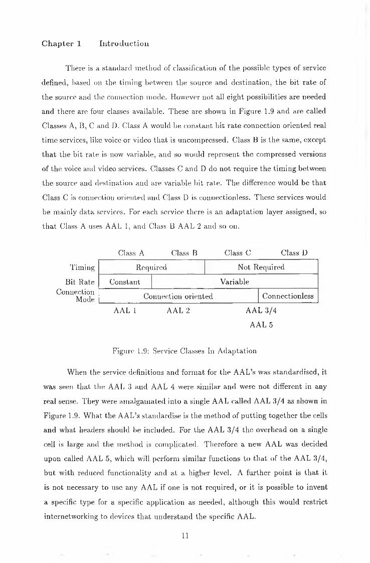
There is a s tandard method of classification of the possible types of service defined, based on the tim ing between the source and destination, the bit ra te of the source and the connection mode. However not all eight possibilities are needed and there are four classes available. These are shown in Figure 1.9 and are called Classes A, B, C and D. Class A would be constant bit ra te connection oriented real t im e services, like voice or video tha t is uncompressed. Class B is the same, except th a t the bit rate is now variable, and so would represent the compressed versions of the voice and video services. Classes C and D do not require the t im ing between the source and destination and are variable bit rate. T he difference would be tha t Class C is connection oriented and Class D is connectionless. These services would be mainly data services. For each service there is an adap ta tion layer assigned, so th a t Class A uses AAL I, and Class B AAL 2 and so on.
Class A Class B Class C Class DTiming Required Not Required
Bit Rate Constant VariableConnection
Mode Connection oriented ConnectionlessAAL 1 AAL 2 AAL 3 /4
AAL 5
Figure 1.9: Service Classes In A dap ta tion
When the service definitions and form at for the A A L’s was standardised , it was seen that the AAL 3 and AAL 4 were similar and were not different in any real sense. They were am algam ated into a single AAL called AAL 3 /4 as shown in Figure 1.9. W hat the AAL’s standardise is the m ethod of p u tt ing together the cells and what headers should be included. For the AAL 3 /4 the overhead on a single cell is large and the m ethod is complicated. Therefore a new AAL was decided upon called AAL 5, which will perform similar functions to th a t of the AAL 3/4, bu t with reduced functionality and at a higher level. A further point is th a t it is not necessary to use any AAL if one is not required, or it is possible to invent a specific type for a specific application as needed, although this would restrict internetworking to devices tha t understand the specific AAL.
11

C h a p ter 1 In tr o d u c t io n
1 .2 .5 A T M S ervicesATM will provide a Quality Of Service ( QOS ) to connections. During connection se t-up there is a need to find agreement between the user and the network on what QOS is required by tha t connection. The user will in itia te a connection request to the network for a connection. The signalling would involve the user passing traffic param eters to the network, which in the ATM Forum 3.0 s tandard [4] is carried in the ATM user cell ra te information element. Here the forward and backward param eters are specified, with param eters like the peak cell rate, the sustainable cell ra te and the m axim um burst size being typical. T he network may adjust the param eters of the connection, if due to other connections Q O S’s, it would not be possible to connect the new connection. It will then be a m a tte r for the user to decide if those param eters are sufficient for the connection or not.
There are a num ber of QOS th a t have been defined and they are coupled with the type of AAL th a t is used. It is of course also possible to have an unspecified QOS with no network guarantees. There are a num ber of types of services tha t can be supported by using these QOS types and the AAL’s. The Constant Bit R ate ( CBR ) service is one tha t uses AAL 1 and requires a level of QOS from the network by specifying the mean bit ra te and the cell loss acceptable as well as the allowable j i t te r in the cell delay. Another type of service is the Variable Bit Rate ( V B R ) service, which will use the AAL 2 and will also require a QOS from the network. In this service there will be specified param eters similar to the C B R but also the burst length and burst tolerance and the peak cell rate. Another type of service is the Unspecified Bit R ate ( U B R ) service, where there is no bit ra te declared and therefore only an unspecified QOS is given to the service. To allow for some guarantees to be given a new type of service called the Available Bit R ate ( ABR ) service is being defined. This service will try to fill up the available bandw idth and still give guarantees to the services.
12
C h a p te r 1 In tr o d u c t io n
1.3 G uarantees In A T M N etw ork sThe main reason th a t congestion and control are im portan t issues in ATM, is th a t in ATM the network is both a ttem pting to give a QOS to the users, as well as multiplexing the users together for efficiency. This is unlike any o ther da ta network at present. Two different types of congestion and control are possible in ATM networks, one at the cell level and the o ther a t the connection or call level. Cell level effects are due to the possible simultaneous arrival of a num ber of cells from different sources. The effect of this is th a t if there is not a buffer large enough to store these cells until they can be served, then there will be loss of cells. At the connection level there are similar problems, except this t im e it could be not only the simultaneous arrival of a num ber of bursts from sources, bu t it could also be tha t the statistical na tu re of a num ber of sources do not interleave to allow the traffic to be smoothed. Congestion of course could also occur a t e ither the cell or connection level due to the sources not correctly specifying or adhering to the param eters tha t were agreed on in the contract. Congestion occurs when not enough resources are available whereas control is the action taken to e ither ensure th a t congestion does not occur, or the action taken when congestion occurs. Connection and cell level control as well as cell level congestion are discussed in the standards [4].
1.3.1 Q uality O f Service D efin ition sA num ber of param eters are used to define the QOS. These include the Cell Error Ratio, Cell Loss Ratio, Cell Misinsertion Rate, Cell Transfer Delay, Mean Cell Transfer Delay, Cell Delay Variation and the Severely Errored Cell Block Ratio. A num ber of classes of QOS are supported by the network and fall into either a Specified QOS or an Unspecified QOS class [4]. At present the standards only specify th a t the Specified QOS class 1, which is the circuit emulation service and constant bit ra te video, be supported. A specified QOS may have two cell loss objectives, for the high and low priority traffic. T he network gives the user no guarantees in the unspecified QOS class. However the user m ay give the network some traffic param eters , tha t the network can use for internal operation. The
13

C h a p ter 1 In tr o d u c t io n
network could then use these param eters internally to achieve some quality of service. These param eters can change during a connection and may not always be specified correctly. This type of traffic could be the so called best-effort traffic. This allows the network to respond to tim e variable resources. The unspecified QOS is optional for the network to support.
Degradation of QOS may arise for m any different reasons and one of these is the ATM switch. The buffer capacity could be a complex multiple queue system with an algorithmically defined service rule th a t could be based on priorities. The switch may thus introduce loss under heavy load. For compliant connections the QOS will be supported for at least the num ber of conforming cells as specified in the conformance definition. For non-com pliant connections the network does not need to support any QOS. The issue arises, when using VPs and VCs, as to what QOS does the network take note of. In other words the users are specifying the QOS on the VCs, bu t the network really only wants to be concerned with the VPs for ease of m anagem ent. The translation between these is specified in the standards and is tha t the QOS of a VP will be the s tric test set of QOS of any underlying VC [4]. This imposes a difficult requirement on the network, in th a t even if only one of many VCs has a hard QOS, the whole VP, and hence all the underlying VCs, are given th a t QOS.
1.3.2 C ontract B etw een U ser & N etw orkThe method used by ATM networks to provide QOS to the users is by m aintaining a contract with them . W hen a connection requires resources there is a contract se t-up between the network and the user. The user describes the connection in terms of network param eters and the network then uses a connection admission control scheme to calculate if the. connection can be adm it ted to the network while providing tha t QOS to the incoming connection and also to m ainta in the QOS to the other connections tha t are already se t-up . One way of achieving this is by using the concept of effective bandwidths, where the burstiness of the connection is captured in a single param eter. There is then a linear constraint on the connection admission control scheme for the connection th a t is about to be adm itted
14

C h a p ter 1 In tr o d u c t io n
and it does not depend recursively on the connections tha t are se t-up . Once the connection is in place it is im portan t for the network to ensure tha t the connection is abiding by the contract. This is done by policing the connection to check on the contract traffic param eters [20]. T he likely m ethod of doing this for bursty connections is by means of the leaky bucket or generic cell ra te algorithm [4, 20]. This algorithm allows cells to pass at the mean rate, bu t also to have some burst characteristics.
Once a contract is in place it is then likely tha t the user will use this inform ation to control their own source. This type of behaviour is called traffic shaping and is similar in na tu re to the policer and usage param eter control th a t the network provides. However a difference is th a t the algorithm does not lose cells tha t do not comply, bu t merely stores then for further transmission and is called a regulator [16]. It is possible tha t the network may provide other contracts where there might be multi-level priority control on the basis of the VC tha t is in use and not the CLP bit in the header. This could be achieved through the signalling at the connection set-up, as is achieved in a num ber of early ATM switches.
1.4 T h e N etw ork &: U ser P ersp ectives
1.4 .1 T h e U ser P ersp ec tiv eThe user perspective on Integrated Services Networks are discussed first to em phasise th a t user preferences should be the prim ary consideration. Once the network is in place only the users directly benefit from using it, by running applications which achieve higher-layer com munication goals. Network owners and operators benefit indirectly, by providing services tha t users want or are willing to pay for.
From the users point of view, there should be as few restrictions as possible on the communication services they obtain from the network. In particu lar :
• the network may ask for various traffic param eters prior to accepting a connection. A user should be able to specify any values for these param eters or simply specify nothing abou t the traffic their connection will generate.
15

C h a p te r 1 In tro d u c tio n
• a user should be able to dem and any values of the various QOS param eters th a t the network has defined; or simply tell the network to provide the best possible service with no guarantees required.
• a user should be able to adjust connection traffic param eters dynam ically during the connection lifetim e, if desired. For example some da ta transfer applications are flexible regarding the delay incurred in completing the transfer and can vary the input traffic ra te during the connection.
• perhaps most importantly, the user should have a sim ple interface to the network to conduct these negotiations.
The simple interface is the interface between the person and the equipm ent tha t they use, and this allows some complexity to be handled by the user’s application hardware or software before the network interface. Therefore the restriction to a simple user interface to the network can be relaxed to a simple hum an interface as is shown in Figure 1.10. Any complicated processing necessary to trans la te user com m ands into actions affecting their network connection is assigned to the local processing element.
Simple Human User / NetworkInterface Interface
Figure 1.10: User Interface
This flexibility in user service characteristics is m otivated by the observation th a t it is becoming more and more difficult to accurately define a “typical” u ser’s requirements. There is already a spectrum of such user traffic characteristics as m ean b i t - ra te or p eak -to -m ean b i t - r a te ratio. In addition, technological advances m ay continue to change the requirements for p resen t-day services, for instance by reducing the bandwidth needed for voice or V C R -quali ty -v ideo calls. There is also a wide range of user QOS requirements even within m any of the service classes proposed in the literature. For example, some “video phone” users m ay require a
16
C h a p ter 1 In tr o d u c t io n
high-quality reliable connection while others m ay be satisfied with poorer-quality or interruptible connections.
1.4 .2 T h e N etw ork P ersp ectiv eAn Integrated Services Network could range from a Local Area Network ( LAN ) to a world-wide W ide Area Network ( WAN ), and could be private ( all the applications controlled by one organisation ) or public. T he operation of a public network may be the responsibility of several organisations, within each of which the operational functions may be au tom ated and / or d istributed. Conceptually, however, the control and m anagem ent functions of an In tegrated Services Network can be associated with a network operator as if one entity was responsible for controlling and operating the network.
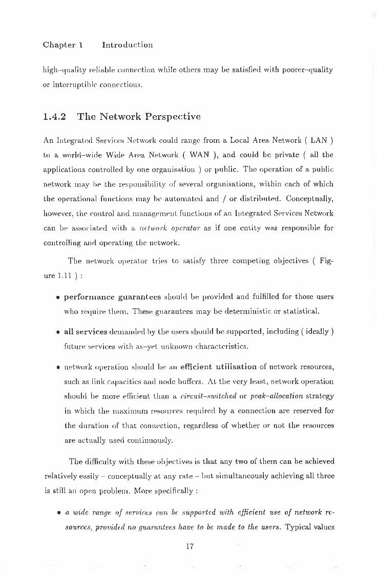
The network operator tries to satisfy three com peting objectives ( Figure 1.11 ) :
• performance guarantees should be provided and fulfilled for those users who require them . These guarantees may be determ inistic or statistical.
• all services dem anded by the users should be supported , including ( ideally ) future services with as-yet unknown characteristics.
• network operation should be an efficient utilisation of network resources, such as link capacities and node buffers. At the very least, network operation should be more efficient than a circuit-switched, or peak-allocation strategy in which the m axim um resources required by a connection are reserved for the duration of tha t connection, regardless of w hether or not the resources are actually used continuously.
The difficulty with these objectives is tha t any two of them can be achieved relatively easily - conceptually at any ra te - b u t simultaneously achieving all three is still an open problem. More specifically :
• a wide range o f services can be supported with efficient use o f network resources, provided no guarantees have to be made to the users. Typical values
17

C h a p ter 1 In tr o d u c t io n
GUARANTEES
SERVICES ► UTILIZATION
Figure 1.11: Network Objectives
of network performance measures may be a good indication of the expected QOS, aggregated over tim e and all users, but some user applications require more specific guarantees.
• guarantees can be made to the users and network operation can be efficient, provided only one ( or a narrow range ) o f service types have to be supported. Focusing on one type of service allows the network to be optimised to efficiently deliver tha t service in the ways required by the users. This is essentially the traditional telephone network model.
• a wide range o f services can be supported, and guarantees demanded by the users can be offered and fulfilled, provided efficient network operation is not important. This is usually achieved by an over provisioning of resources, such as reserving the peak bandwidth required by a connection.
The network operator should also be able to offer more customised service to individual users than is usually available today. This means th a t traditional network performance metrics such as average delay or packet loss m ay not be fine-grained enough, since typically a user cares only about the QOS their connections receive. Advances in user hardware and software, and the development of a com petitive network provider industry, will require network operators to focus on satisfying the communications needs of an individual user, regardless of the size of the user’s connection.
18

C h a p ter 1 In tro d u ct io n
1 .4 .3 Future In tegrated —S ervices N etw ork sT he exact form of integrated-servic.es networks of the fu ture is also unclear, but based on current trends in communications and com puting it is possible to predict some of its features with reasonable confidence. M ultim edia services offering storage and transfer of voice, video, images and d a ta will be supported , allowing rem ote conferencing and collaboration and replacing tex t processing with multi- m edia ‘docum ent’ processing. Networks will be interconnected and will allow users and organisations to set up virtual private networks em bedded in the physical network [2, 74], Intelligent network interfaces will be needed at internetwork boundaries and at user access points to hide the interface details and present the image of a single network to the users. The implication of this is th a t the boundaries of the network become more complex while the interior of the network becomes simpler. The users will also have become more complex com pared to the sort of user tha t would have typically used these networks. Users will dem and a wide spectrum of application requirements as they become familiar with the network. Some may continue to opt for network-defined services or choose from a library of predeterm ined services, bu t others may want to customise their connections and vary connection param eters dynamically.
The view taken here is th a t current trends and fu ture considerations in the communications and com puting areas point to the need for a change in the traditional user-network relationship. The traditional model is centralised with passive users : the network provides well-defined services and users choose from this limited range. User feedback is long-term and inferred from the aggregate dem ands for services. For example the feedback m ay take the form of the users either not re-c.onnecting to tha t service or changing to ano ther service, in a time period tha t is larger than maybe hundreds or thousands of call times. Because of the small well-defined services th a t the network provides, the network can assume th a t the users are identical in characteristics, and so when getting feedback will average the response out over all the. users. This is appropriate for large-scale provision of a single service, as in the phone network, bu t m ay be unsuitable for the kind of integrated m ulti-service network described above. T he relationship
19

C h a p te r 1 In tr o d u c t io n
implied by many of the proposed CAC schemes is more of a ‘con trac t’ : users describe their traffic and make quality dem ands, and the network provides a s ta ted level of service while enforcing the user com m itm ents. Some problems with this model were outlined above, although it is a step in the right direction. Taking this process further, the view here is th a t :
• the network should be a provider of basic network resources ra the r than complex user services;
• the responsibility for packaging these resources into services should lie with the users ( or in rea l- t im e their interface equipm ent );
• the network’s prim ary function should be to co-ord in a te requests for its resources. The goal of this co-ordination could be to optimise some measure of network performance, or to maximise a suitably-defined global user satisfaction, or to ensure some degree of fairness, or some other objective.
Thus the network is viewed simply as a h igh-speed cell relay network in which the central issue is transporting cells ra ther than implementing services [46]. Furtherm ore ATM is supposed to be a service independent network and therefore should not be concerned with the services tha t are im plem ented at the higher layers b u t instead concentrate on the core issue of cell delivery. Users may actually be working with higher layer protocols such as T C P / I P running on top of an ATM network, which also argues for keeping the ATM network as simple as possible. One proposal along these lines is to move connection admission and bandw idth allocation decisions to the term inal equipm ent a t the network access points, and somehow ensure tha t the combined user rates do not exceed the network capacities [81]. This gives a simpler network but it may be less efficient than previous networks.
Here the users take responsibility for requesting sufficient network resources to meet their QOS requirements. At connection se t-up this involves specifying some param eters of the requested connection, e ither manually or in a m enu-driven environm ent. If users want to adjust connection param eters during a connection then these param eter specifications m ay be autom ated . This kind of in-connection
20

C h a p te r 1 In tr o d u c t io n
negotiation is desirable for bursty connections where the actual resource usage is of interest [70]. One traffic managem ent scheme for burst- level resource reservation is described in [80], and a form of in-connection negotiation is now commercially available in some network interface equipm ent. Even for static connection requests, the connection se t-up process may involve a negotiation between the user and the network in which the user modifies their request to conform to the current level of resource utilisation. For example [25] outlines a rea l- t im e channel se t-up procedure in which detailed information is sent to the user if a connection request is refused, allowing the user to take this feedback into account in a revised request.
Some work is underway on modifying user traffic inputs via pricing in the In ternet [51] and in integrated-servic.es networks [6 6 , 76]. A con tract-based CAC scheme is proposed in [40] in which the. charge to users is related to how accurately they declared their traffic, rewarding users who provide b e t te r information on their connection characteristics.
1.5 R esou rce A llocation O f A T M N etw orksThere are many resources in ATM networks and the ones th a t are of interest here are the buffer spaces and bandwidths tha t are available in the network. The resources issue at the connection level is how to achieve reasonable network efficiency for source types, where traditional resource allocation techniques may not apply. Reactive control and feedback schemes are under investigation ( e.g. [27, 38] ) and may be useful in certain network environments or on longer t im e scales, e.g. connection level ra ther than burst or cell level. Experience with real users will show which schemes are feasible in an actual network as opposed to a research or test environm ent. The problem is complex and is likely to require a multilevel solution approach [47, 60, 85]. It is fair to say th a t how bandw idth will be allocated in ATM networks is still an open question. There is also some work on the cell level resource allocation in terms of the overhead and efficiency of the throughput of the cells.
21

C h a p ter 1 In tr o d u c t io n
1.5 .1 T im e ScalesThere are a num ber of t im e scales tha t are relevant in ATM networks and there are very different approaches used to examine each of them . The smallest time interval is concerned with bit tim ing and whether the bits are correct or not. This bit scale level is shown in Figure 1.12, and this is relevant at the physical m edium sublayer and is on the sub micro-second scale.
"S' J ?C% S'
Time
Figure 1.12: T im e Levels In ATM Networks
The cell scale effects are ones tha t are relevant to how the cells are put together, with particular im portance being placed on the overhead in the cell. This is discussed in C hap ter 3, when the overhead within the cell is too large over satellite links. The burst scale is relevant when dealing with the tim e between cells from the same source and how cells from different sources are mixed or multiplexed together. This is also dealt with in Chapter 3 in term s of what the worst case traffic might be due to cell effects. The connection scale is on the level of milli-seconds or more and this is what the remaining chapters deal with. There are longer time scales like the call scale, but these are not covered here. All these tim e scales can be seen in Figure 1.12.
W hen dealing with a particular tim e scale, especially the longer ones, it is im portan t for simulations to make a num ber of approxim ations about the lower tim e scale effects. W hen the connection level is dealt with it is convenient to make assumptions tha t there are no cell scale or bit scale effects tha t impinge on the model. If this were not the case then the t im e taken and complexity involved in simulation would be large and so would be unfeasible or impractical.
22

C h a p te r 1 In tr o d u c t io n
1.5 .2 S ta tistica l M u ltip lex in gOne of the fundam ental issues which has not yet been satisfactorily resolved is the mechanism by which user traffic, will be accepted into the network, usually referred to as Connection Admission Control ( CAC ). W hen a new connection is requested by a user, the network m ust decide whether or not to accept the connection; and if so, how to route it through the network and what resources to reserve for its virtual channel. Packet-sw itched networks use higher-layer protocols to guarantee acceptable packet delivery but these are not expected to scale well to broadband speeds. In circuit-switched networks ( such as most telephone networks ) the CAC mechanism results in connection blocking when the bandw idth of a requested connection exceeds the available bandwidth [5]. But in an integrated-services network the traffic source may be bursty, so the required bandw idth of its v ir tual channel varies with tim e during the connection.
The natu re of this tim e-vary ing behaviour and the m ean bandw idth requirem ent vary widely among different sources. Therefore it is difficult to characterise the bandwidth of a requested connection. This difficulty has led to proposals to reserve the peak bandw idth of the connection ( determ inistic multiplexing ), as required for constant bit rate. ( C B R ) sources. However the gain in efficiency possible by taking advantage of the statistical na tu re of variable bit ra te ( V B R ) sources has led to many schemes for statistical multiplexing. Such schemes assign less than the peak bandwidth required, and therefore may introduce cell loss and / or delay. The extent to which these service degradations occur is measured by the quality of service ( QOS ) offered to the connection.
The aim of a preventive CAC scheme is to balance the QOS offered to adm itted connections against network utilisation by limiting the num ber of connections using the network. Many schemes described in the l ite ra ture decide w hether or not to accept a connection based on knowledge of the connection behaviour, the user’s quality requirements, and the current state of the network [35, 69]. An example of this is given in [69], where the connection behaviour coupled with the QOS are m apped to specific, traffic classes. The current s ta te of the network is gained by
23

C h a p te r 1 In tr o d u c t io n
using predictive methods as well as reactive controls from the network. Another example is tha t the traffic contract tha t the user and network agreed on, must be available to the CAC [4] so tha t the CAC can base i t ’s decision on the connection behaviour and the users quality of service requirements. The network might then use a theory like “effective bandwidths” , which tells the CAC the current state of the network, to calculate if the connection can be carried without effecting the o ther users. Ideally a user requesting a connection would give a com plete statistical description of the connection, but in practice only a l im ited indication of expected connection behaviour is feasible [SO]. Connection behaviour is described by a set of param eters called traffic descriptors, such as m ean bit rate, peak b it rate, m axim um burst length, probability of cell arrival in a fixed interval, and so on. User quality requirements are usually expressed in term s of acceptable cell loss, delay and j it te r . Based on these requirements, traffic sources are divided into classes and each class is provided with a different QOS guarantee, eg. [79]. T he current s ta te of the network can be determ ined by m onitoring the utilisation of network resources and /o r by characterising the behaviour of connections already adm itted . For example, traffic, models based on fluid flow approxim ations have been used in analysing network bandwidth and buffer utilisation [48]. Based on the above knowledge, CAC schemes have been developed in which each source is assigned an effective bandwidth [39] in order to meet its QOS while still perm itting a statistical multiplexing gain.
1 .5 .3 E ffective B an d w id tlisEffective bandwidths are a way of summarising the statistical information of a source in a single param eter. The complex problem of resource allocation of a m ulti-service network can be simplified by try ing to get an equivalent circuit switched model [21]. By using effective bandw idths it is possible to get a linear equation similar to the circuit switched networks and see if there is sufficient bandwidth left to adm it another connection. The original idea of effective bandwidths can be a ttr ibu ted to Hui [36] and a sum m ary of the uses can be found in [39]. Using tha t notation, here is an overview of the m athem atica l formulation.
24

C h a p ter 1 In tr o d u c t io n
The simplest model is tha t there are J sources th a t are sharing the same link which has a capacity of C. Let X : be the load produced by source j and assume tha t all the X j 's are independent random variables with possibly different distributions. T he performance constraint on the system s can be given by looking at the probability of overflow of the queue and this is equivalent to the question whether it is possible to impose conditions on the distributions of the X j 1 s which would ensure th a t :
(1.1)
for a given value of 7 ? The answer is th a t there are constants a and K tha t depend 011 7 and C such tha t if :
■ £ B ( F j ) < K (1.2 )j - 1
is satisfied then Equation 1.1 is also satisfied. This is ju s t a linear constraint. The variable B (F j) is called the effective bandw idth and is given by :
B (F j) = ~ log E [e”A'<] (1.3)a J
This effective bandw idth can now be trea ted like in the circuit switched network and it is possible for a large range of m u l t i - ty p e sources th a t share a single queue to have a linear constraint 011 performance. This is true because it is possible to have an asymptotic, constraint 011 the tail d istribution of the buffers workload [2 1 ]. It is now known [40] tha t for a quite general models of sources and resources it is possible to associate an effective bandw idth to each source, such th a t if the sum of those effective bandwidths using the resource is less than a critical value then the resource can deliver the required perform ance [82]. For more general models of sources the simple version of the effective bandw idths given in Equation 1.3 may not be valid, however it is not known when the more general effective bandwidth is needed.
25

C h a p ter 1 In tr o d u c t io n
1.5 .4 C urrent R esou rce A lloca tion T echniquesThe current resource allocation methods used for services in ATM rely on many techniques. At present the CBR traffic and circuit emulation traffic is decoupled from the remaining services. This is achieved by using different VPs for each of them. This allows each sub-problem to be tackled independently. Effectively the bandw idth for the C B R traffic is split from the o ther traffic’s bandwidth , by reserving the am ount needed in advance. The o ther traffic can then have no effect on the CBR traffic. However not all the advantages of s tatistical multiplexing can be got by doing this. For VBR services like compressed voice there are a num ber of models using effective bandwidths tha t look to be useful and provide good bounds for the connection admission control. The C B R and V B R services will be policed by either a single leaky bucket or possibly a dual leaky bucket.
ABR traffic is more difficult to control due to the unknown na tu re of the sources and there have been a num ber of proposed schemes [1 0 , 6 8 ] to control it. The factors th a t have influenced the decisions on the choice of schemes are numerous and vary from what types of sources are expected to what might be possible in real networks. The final decision might not even have been arrived at, and this area is still under intense research.
An early scheme proposed, is to ju s t allocate the resources for the peak rate and resign the network to inefficiency. However this is probably only a short term solution as com petitive forces will force this option out. There is also the possibility of offering different levels of priority tha t the user can allocate to different services tha t they might have multiplexed together. W hile this might work when the user is in control of the multiplexing, in bigger networks this m ight not be possible. The different levels of priority are achieved by having a num ber of ou tpu t buffers in the switch and allocating different VCs to different buffers. As m any as seven levels of priority can be offered this way. The shortcoming of this scheme is th a t it is not clear how to decide to distribute the levels of priority, and different users may give different priorities to the same types of service so making decisions within the network becomes complex. This solution is likely to be of use only in the local part
26

C h a p ter 1 In tr o d u c t io n
of the network.One of the m ajor questions th a t has been posed for A B R traffic, is whether
a closed-loop scheme or an opeu-loop scheme is needed ? T he ATM Forum have decided that closed-loop feedback is needed for A B R traffic. Therefore en d -to -en d feedback is needed, bu t what type of feedback ? There is an ongoing debate about whether a credit based flow control scheme or a ra te based flow control scheme is better [77]. In a credit based flow control scheme it is claimed th a t there will be no loss and there is no need for policing the connections, as the credits are only created when there are sufficient resources available for the traffic. However the ra te based schemes depend on the ability of the A BR traffic to fill up the rest of the bandwidth and these are able to do this at high speed, whereas credit based schemes are not. The ATM forum has specified th a t the ra te based scheme will be the one implemented. Another question is how does the feedback actually take place, is it bit based or explicit ? W ith the bit based schemes the bit could be contained in the cells bu t then there has to a rule to decide w hat to do in each case of receiving this bit. However in the explicit case the new adjusted ra te is specified, bu t it needs a resource m anagem ent cell to carry the information. However this explicit feedback is the preferred m ethod. It is also likely th a t ra the r th a t using queue length to measure congestion, the rate of queue growth will be used.
Two schemes tha t have been tested are the Explicit Forward Congestion Indication ( EFCI ), scheme and the Enhanced Proportional R ate Control Algorithm ( EPR C A ). The EFCI scheme is similar to a scheme tha t was used in other data networks, and is a bit based feedback scheme. T he EPR C A scheme is on the other hand a new scheme and uses the resource m anagem ent cells to send information from the switches to the end users, in order to control the sources.
1.5 .5 W ill R esou rce A llo ca tio n C ontinue To B e Im p ortan t ?Some com mentators have suggested tha t the widespread deployment of fiber optic lines, and continuing exponential decreases in processor and m em ory costs, will result in these network resources becoming essentially “free” so th a t efficiency in
27

C h a p te r 1 In tr o d u c t io n
their use will not be im portan t in the future. However three points should be kept in m ind :
1 . demands are continuing to increase exponentially, so th a t it is not clear when - if ever - network resources will be “free” ;
2 . past experience suggests tha t application developers will have no difficulty in designing new services tha t use up all the available resources, perhaps after an initial ad justm ent period ;
3. when a significant num ber of users become involved in defining their service characteristics, efficient network operation will be critical in a com petitive network provider environment. P u t simply, if network operation is not efficient, the users will be efficient - by multiplexing their traffic before subm itting it to the network, for example. Legal barriers or tariff disincentives to this kind of user behaviour may not be feasible, so network inefficiency could lead to a financial penalty for the network operator.
1.6 A N ew M o d el O f A T M N etw ork in gAlready the model for ATM service negotiation involves the users more than before in defining their own services. Taking this process further, the following basic principles of network operation are proposed :
• the network should be a provider of resources ra ther than services ;
• responsibility for packaging these resources into services should lie with the users, or in rea l- tim e their interface equipm ent ;
• the network, or a third party provider, m ight offer a pre-defined menu of services th a t the users can choose from, if there are enough users th a t do not want to define their own services ;
• the network’s p rim ary function should be to co-ordinate requests for its resources. The goal of this co-ordination could be to optimise some measure
28

C h a p ter 1 In tr o d u c t io n
of network performance, or to maximise a suitably-defined global user satisfaction, or to ensure some degree of fairness, or some other objective ;
• resources can be requested and allocated in rea l- tim e, or essentially continuously. Therefore for all but the shortest-l ived connections it should be possible to adjust a connection’s param eters during its lifetime.
In this model the network is simply a h igh-speed cell-relay network [67] in which the central issue is transporting cells ra the r than im plementing services required at higher levels. This view is consistent with regarding a VC connection in an ATM network as a virtual wire [22], since the functionality delivered by the VC is similar to th a t of the physical layer in the OSI reference model. An im m ediate consequence of this new model is a fundam ental change in user-netw ork interaction : more flexible “contracts” can be continuously renegotiated by those users whose applications or QOS preferences perm it it, while still accom m odating users whose demands can be met by pre-agreed contracts.
The model proposed here agrees with the spirit of recent proposals to move decisions about network services to the edges of the network, preferably all the way to the users, and to take advantage of the flexibility of some application types :
• the proposed Available B it-R a te ( ABR, ) service would assign whatever bandw idth is not currently allocated for reserved-bandw idth applications to those users whose applications require little or no guarantees on delay or cell loss ;
• some proposed video schemes divide the bandw idth assigned to a connection into base and enhancement layers. The base layer bandw idth would be guaranteed so th a t some m inim um service is obtained, while the enhancem ent layer would provide additional bandw idth ( which presum ably corresponds to improved service ) whenever it was otherwise unused ;
• even for pre-agreed connection requests, the se t-u p phase could involve an iterative negotiation between the user and the network in which the user modifies their request to conform to the current level of resource utilisation.
29

C h a p ter 1 In tr o d u c t io n
For example [25] describes a rea l- tim e se t-u p procedure in which detailed information is sent to users whose connection requests are refused, allowing them to take this feedback into account in a revised request.
The crucial issue ignored in most of these proposals is the basis on which decisions should be made, both by the network and by users. By developing an economic framework in which incentives are provided, it is possible to make rational decisions and resource allocations in real- tim e. These incentives could correspond to actual money, or could simply be control signals, provided the users and the network operator react appropriately to them ( for example in a private network where one entity controls both the network and the “users” i.e. applications ).
1.7 O b jectives of T hesisThe main objective of this thesis is to propose m ethods to increase the efficiency of ATM. There is the way in which the ATM cell is formed and then multiplexed together in a buffer. The way tha t the cell is pu t together can lead to a gain in efficiency as is shown when looking a t ATM over satllite links, and the way the cells are multiplexed together is im portan t as can be seen when examining the area of worst case traffic in the network, over satellite, due to the inefficiencies. Another area of interest is tha t of user behaviour and it is shown th a t when adaptive users are examined it is possible to increase the efficiency of the network. There are a num ber of objectives for each chapter and these are now described.
1.7.1 O b jectives o f C h apter 2The objective of C hap ter 2 is to develop the tools for the further chapters. These tools are the models of the sources th a t will be used to investigate various aspects of ATM networks and the modelling and simulation techniques needed because of the nature of ATM networks. There is first a motivation to dem onstra te what sort of models are useful when examining ATM networks. It is seen th a t ATM networks pose some different simulation problems com pared to other networks and the so
30

C h a p ter 1 In tr o d u c t io n
lutions to these are a ttem p ted . There follows some justification for the simulation methods tha t are used in the rest of the thesis. There is some detail given about the software and simulation platform th a t will be used. T he different models designed are models for voice, video and d a ta sources, as well as models for the different network functions th a t will be. needed in the rest of the chapters.
1 .7 .2 O b jectives o f C h apter 3The two issues dealt with in C hap ter 3 are firstly the m ethod in which the cell is formed and secondly the way tha t cells can be multiplexed together. The first objective was to send d a ta efficiently over a satellite link along with o ther services, like voice. One of the problems is tha t there might not be a higher layer protocol protecting the d a ta from errors th a t would be encountered on the satellite link. W h at is then seen is tha t when using satellite hops, it is not possible to use the normal type of ATM protocol. However with some changes to the AAL, it would be possible to easily send d a ta reliably across the satellite. T he changes have to do with the m ethod by which the cell is formed.
Another problem, again concerned with the cell level, is to exam ine if there is a type of source, tha t adheres to the ATM policer, called the leaky bucket, tha t imposes the biggest constraints on the network. P u t another way, is there a type of source tha t complies with the leaky bucket and produces the worst performance in the network. If this were to be true, then for modelling purposes, it would be possible to always use this type of source, knowing tha t for all o ther types of sources, the network performance would be better . Two sources have been suggested to be contenders for being the. worst case source and what is shown here is th a t neither of these is the worst all the time. This of course does not rule out the possibility of there being an as yet unknown source tha t is indeed the worst case, b u t ra ther it tells tha t both types of sources should be considered when looking at performance modelling.
31

C h a p ter 1 In tro d u c tio n
1 .7 .3 O b jectives o f C hapter 4The objective of C hapter 4 is to define the problem of congestion control and propose solutions to it. Even the definition of congestion is unclear, and so a m athem atical framework is proposed to deal with these issues. T he m athem atica l model tha t is employed is based on economic principles, and this allows us to strictly define congestion and also efficiency in economic terms.
The user types are re-defined by using the idea of adaptive param eters, giving a new set of classification of users. By using the re-defined user types and the economic framework developed, it is possible to investigate how an economic solution to congestion, by using pricing, compares against o ther schemes. To define the efficiency, consideration has to be given to both economic term s and network terms. There are two types of efficiency present, network efficiency and economic efficiency. Some simple models and simulations are presented and the results show th a t by using both pricing and adaptive users, both the network and economic efficiency increase at the same time.
1.8 Sum m aryThis chapter has dealt with the need for ATM in Section 1.1 and has then developed the current standards tha t have been applied to ATM in Section 1.2. There the basic terminology has been introduced and explained. In Section 1.3 the framework for discussing guarantees in ATM was introduced and in Section 1.4 the user and network perspectives were addressed. In Section 1.5 the current and fu ture methods of resource allocation was presented. T he new model of ATM networking was explained in Section 1.6 and the sum m ary of the rest of this work in Section 1.8 concluded this chapter.
1.8 .1 Sum m ary o f T h esisTo analyse and compare various ideas in ATM networks it is usual to try to model and simulate the system. The models th a t are needed for this work are the typical
32

C h a p te r 1 In tr o d u c t io n
types of sources tha t might be used in future, and the parts of the network tha t are relevant to the performance of those services. This is dealt with in C hap ter 2 where various video sources, as well as d a ta and voice sources, are presented. A discrete event simulator is introduced and the simulation models are verified and validated.
At the level of ATM cells there are two im portan t issues dealt with, how to pu t the cell together and how to pu t the cells into the network, and these are examined in C hap ter 3. An example of why the form ation of the ATM cell is importan t is given by way of an example, which is a satellite link. This satellite link is modelled and then simulation carried out to exam ine the performance of the ATM cells with suggestions as to how the performance might be improved. The way tha t the cells are inpu tted to the network, and still abiding by the congestion control algorithms, is an im portan t issue, for network design. T he different ways of achieving this are then examined and some conclusions are drawn from m athem atica l analysis.
The different types of users th a t will use the ATM networks are presented in C hap ter 4. There are new types of sources presented and, even without giving a traffic descriptor, these types can still get guarantees. These adaptive sources are then modelled mathematically. A new model for efficiency is presented, where both network issues and economic issues are dealt with. By using economic principles it is possible to gain advantages com pared to the traditional approach in term s of efficiency. T he economic framework can also take advantage of the adaptive types of sources. Finally in C hap ter 5 some conclusions are drawn from the previous work.
33

Chapter 2
Perform ance M odelling Sz
Sim ulation
2.1 In trod u ctionT he Asynchronous Transfer Mode ( ATM ) network is widely accepted as being the broadband network of the fu ture [20, 46]. ATM allows the design of networks tha t give efficient and flexible allocation of resources by only allocating the am ount of the resource th a t is needed. This ability of ATM networks to support variable bit rate traffic can be used to meet the dramatically changing traffic requirements of many applications such as video telephony, full motion video or h igh-speed d a ta transfers. New im portan t issues related to ATM networks, such as congestion control and cell loss probability, have to be investigated. In addition even though the ATM concept provides ‘bandw idth on d em and 1 there is a need to ascertain the network’s efficiency or throughput. Performance evaluation of ATM broadband networks can be addressed by simulation studies using realistic and accura te models.
The modelling and simulation of ATM networks presents new challenges due to the small packet size and the high bit rate of the link. If reasonable run times are to be achieved on reasonable computers then ways of making the simulation efficient are essential. There are m any approaches to this problem, bu t here two m ethods will be investigated, decomposition and ra te control m ethods. By using these enhancements it is possible to achieve bo th accuracy and quick simulation
34

C h a p ter 2 P e r fo r m a n c e M o d e l l in g & S im u la t io n
time.This chapter is organised as follows. There is a discussion of modelling
and in particular network modelling in Section 2.2. One of the main objectives of the modelling was to model the different source types and this is addressed in Section 2.3. In this section the video source model is concentrated on as this presents the most difficulties. To produce an accurate video model the first task is to characterise the d a ta collected and this is addressed in Sub-Section 2.3.1, along with data for voice and d a ta models. The models are then presented, first the voice model in Sub-Section 2.3.2, then the video models in Sub-Section 2.3.3 and finally the da ta model in Sub-Section 2.3.4. In Section 2.4 the video model tha t was presented in the previous section is com pared to M P E G models. F irstly in S ub- Section 2.4.1 an overview of M PE G is given, followed in Sub-Section 2.4.2 by a hierarchical view of M PEG models and finally in Sub-Section 2.4.3 by a comparison of M PEG models to II.261 models. After the models have been designed there is a need to convert them in to simulation models. There is a discussion of simulation in Section 2.5. The package th a t was used to build the sim ulation models is called SES /workbench and is described in Sub-Section 2.5.1. This package provides a set of software tools for graphical anim ation and sim ulation of models. T he models th a t were designed in Section 2.3 are converted and described in Sub-Section 2.5.2. T he validation of these models is presented in Sub-Section 2.5.3 along with general discussion of validation m ethods. The next section deals with the problems of simulation in high-speed networks and the problems with m em ory and speed. This is discussed in Section 2.6. There are various techniques for overcoming these problems and these are described in Sub-Sections 2.6.1, 2.6.2 and 2.6.3. Finally there is some discussion of the overall chapter in Section 2.7.
2.2 O verview O f M od ellin gA model of a system is an abstraction and approxim ation to the actual one. The model may be conceptual, physical, electronic or com puter based. A model should simplify the analysis of the system under investigation. T he purpose of modelling is
35

C h a p ter 2 P e r fo r m a n c e M o d e l l in g &; S im u la t io n
to help the analysis, design, control or understanding of a system without actually having to build the system. There are many occasions where the actual system cannot be accessible, such as future systems which are only conceptual, or expensive systems where the cost of using the system is high, or system s th a t are providing critical services and cannot be taken out of use. Telecommunication networks and in particular fu ture networks are ideal candidates for modelling as they are expensive, very large and usually only conceptual a t the stage of modelling. Also it is usually not feasible to build a pro to type due to the inflexibility of the prototype and the expense. The types of systems tha t are modelled fall into these categories, for example a satellite link is an expensive item, or custom er behaviour is hard to work with in practise without long trials. T he models th a t are of interest are conceptual models and use is m ade of them to build com puter simulation models.
There are many factors th a t are taken into account when modelling bu t the most im portan t factor is probably the detail of the model. It is usual to have hard constraints on time, money and com puter resources. It is interesting to note tha t for most modelling one of the m ain reasons is th a t the real system is too slow and it would take too long to wait for results from it. However in the case of high-speed networks it is the opposite and it is difficult to get close to m atching the speed of the real systems by modelling and simulation. A basic principle of modelling is to try and reduce the detail in the model. This has to be done in the context of having the model accurately portraying the essential aspects th a t are of interest to the system. Some of the m ain principles used in modelling in this work are :
• use a big picture initially to find the areas of interest
• find the most im portan t parts of the system
• start with basic small models
• decide what results and performance is required
• only include detail th a t effects the results of the modelling
• include detail only to the extent tha t the d a ta is available
• constantly re-check the model against the aims

C h a p te r 2 P e r fo r m a n c e M o d e l l in g &c S im u la t io n
• it may be necessary to include more detail for credibility
Even if it were possible to build a detailed model, the excessive detail would slow down the run tim e and be irrelevant to the results. The detail in the model should only really represent the detail of the da ta tha t is available to us.
In terms of modelling these systems, the d iv ide-and-conquer approach is taken. Each component of the system is modelled separately and then the resulting model is the combination of these. The main interest of the modelling is for performance and so the elements tha t are modelled effect the performance of the system. Individual elements are the source models and the network elements. There are also other elements modelled such as customer behaviour and perform ance measures. The source models are discussed in detail in Section 2.3. The network elements include the. ATM cell structure , the ATM A dapta tion Layers of interest, the control measures in the ATM user-network interface, the policing methods, various link rates and standards as well as buffers and multiplexors. The result tha t are expected from the models is to be able to build com puter simulation models. These models can then be used to investigate the performance of proposed systems and com pare them to each other. The performance is generally given in terms of delay and loss, bu t also the efficiency, both in term s of networks and economics is investigated.
2.3 Source M o d ellin gThere is a need to model telecommunications elements for network design and planning, such as the investigation of various congestion control mechanisms. Traditionally it was sufficient to model voice traffic for the telephone network and d a ta traffic for com puter networks. W ith the emergence of ATM networks there will be a m ix ture of voice, data , video and still image traffic on one network. The sources may take advantage of the ability of ATM to provide bandw idth on dem and by supporting variable bit ra te traffic. In particular video coding schemes will produce bursty variable bit ra te traffic. W hile there are a num ber of coding schemes proposed it is likely th a t the algorithms used will be similar to those in the
37

C h a p te r 2 P er fo rm a n ce M o d e l l in g &c S im u la t io n
H.261 standard . The work here presents a contribution to the area of Video Traffic Characterisation ( V TC ). Video source models are presented which are based on analysis of real video phone type d a ta and discuss the results of the simulations carried out using these models. Both one and two layer codecs are considered. T he one layer codec is based on a discrete t im e Markov chain while the two layer model is modelled on its individual layers. Both are derived from an analysis of video conference data. The models are simulated using a commercial discrete event simulation tool. Evaluation of the characteristics of each source are presented, as are the capabilities and lim itations of the models. Comparisons are drawn between actual da ta and the models. While the results th a t are produced are dependent on the model of the video codec used, the m ethod used to design the model is general and can be adapted to any codec design. A part from video source modelling there is also a need to model the voice and d a ta sources and these models are also presented.
This section deals with modelling voice, video and d a ta sources for ATM networks. The voice models are taken from the l i te ra tu re [12, 15]. T he video data, which the video models are based on, were generated as in [87] using a H.261 one and two layer codec. This codec produced a d a ta set consisting of bit ra tes for each video frame. The da ta model presented here is for a file transfer application and gives a bursty source. The basis for the model is typical file sizes on a com puter system.
2.3 .1 Source A nalysis A nd C haracterisationVoice has been characterised by a constant bit ra te source, bu t this has been due to the technology ra ther than the information transfer rate. The normal m ethod for digitising the voice signal is to bandlim it the signal to a band from 100 Hz to 3400 Hertz and then to sample th a t at 8 kHz. Each sample is then given 8 bits, to produce a bit ra te of 64 kb/s . A voice call between two people will be silent abou t half the tim e in each direction, unless bo th are going to speak together. It is also possible to remove the inter-word silence and this gives the s tandard model used in the literature [12, 15, 29, 64]. It is possible to achieve about 35-40 percent
38

C h a p ter 2 P e r fo r m a n c e M o d e l l in g S im u la t io n
compression by using both of these silence removal techniques. T he resulting model can be described by a two s ta te on-ofF Markov chain.
Video, like voice, is naturally bursty [12, 15, 29] b u t can be m anipulated to give a constant o u tp u t bit rate. To gain the m ax im um efficiency from an ATM network only the real am ount of information should be sent. This will change as the information content of the p icture changes and so a variable bit ra te ou tpu t from the codec is expected. To gain m axim um compression a single one layer codec could be used. Sudden movements in the picture or scene changes will produce large information transfers and so will produce high b it rates. Small changes from frame to frame will result in low bit rates.
In ATM networks it is sometimes hard to characterise the sources. Performance evaluation of the network becomes difficult and subsequent guarantees of quality of service ( QOS ) are hard to achieve [65]. However a QOS for a constant bit ra te source might be easier to guarantee than th a t of a variable source. This has led to the development of two layered codecs [87]. One layer has a constant bit rate, called the base layer, and delivers a m in im um QOS to the user. The second layer contains the enhancem ent to the base layer and is bursty in nature. The base layer is expected to achieve very low loss rates, m aybe 10E-9 bit error rate, and this can be achieved as the layer is more or less constant b it rate. The enhancement layer can tolerate more loss and will slowly degrade the picture quality. The relevant quality of pictures of the one and two layer codecs is subject to the coding involved in the codecs, the bandw idth available and the probability of cell loss. The empirical d a ta on which the models are based were generated using algorithms implemented as in [87].
The H.261 video codec, is a m ethod of digitising video for use in video conferencing across the telephone network, and so the b it ra te th a t is produced is constant bit rate and is specified by a bit ra te of p 64 k b /s where p = 1,* •• ,30. For p = l a low quality video telephony of 64 k b /s is got, bu t if = 6 to get a bit ra te of 384 kb /s , then a good quality video conferencing is achieved, and of course it is possible to use up to p = 30 to give a b it ra te of 2 M b /s for high quality video.
Some of the m ain elements of H.261 include interfram e and intrafram e pre
39

C h a p ter 2 P e r fo r m a n c e M o d e l l in g & S im u la t io n
diction, motion com pensation, discrete cosine transform ation ( DCT ), quantisation of DCT coefficients and run length coding of the D C T coefficients. Interfram e prediction takes advantage of the fact tha t consecutive frames will be quite similar allowing jus t the difference between frames to be tran sm itted ra ther than the entire fram e data.
Intrafram e compression is when the frames are quite different and the frame is treated independently and compressed in a m anner similar to an image. This is used when there is substantia l new information in a frame, like a t the s ta r t of a video sequence or a sudden motion/scene change.
The II.261 codec produces constant bit ra te video, bu t the m ethod used to code the. video produced is inherently variable bit ra te [87], T he way th a t theH.261 produces a constant bit rate is tha t the quantiser step is adjusted during buffering the o u tp u t of the codec and a constant bit ra te is produced. The picture quality then varies according to the am ount of motion in the sequence shown. If the quantiser step is left fixed then a variable bit ra te o u tp u t is produced, and an approxim ate constant p ic ture quality is achieved. This variable bit ra te codec has a peak to mean of abou t 4 in general [87]. In this work a variable bit ra te one layer codec was produced using this technique. A two layer codec was investigated as well. The two layer codec is produced by using a one layer variable codec and putt ing the more im portan t information into a base layer. Such information might include the picture s ta r t codes, the coding modes, motion vectors and some of the quantised DCT coefficients. This is filled to produce a constant bit ra te layer and will provide a coarse level of quality. The rest of the coding will then, if present, be pu t into the enhancem ent layer, which will be inherently bursty.
The video sequences considered here are of ju s t a single person talking with some zooming motion. This is more typical of a video phone type picture than video conferencing because there is little changing of scenes and only m oderate motion. The spatial resolution of the five m inute sequence was Com mon Image Format, C IF , ( 384, 288 ) and the tem poral resolution was 25Hz. In order to capture the d a ta set for the encoded video sequences, on a per fram e basis, the ou tpu ts of the codecs were sampled every 0.04 seconds. This produced approxim ately 7500
40

C h a p ter 2 P er fo rm a n ce M o d e l l in g &; S im u la t io n
frames to be considered. It can be seen from Figure 2.1 th a t the bit ra te of this one layer codec varies considerably over the tim e interval. This short sequence and the type of p icture th a t was used are limiting factors for the reliability of the models produced.
Bit rate kbps
3Frame number x 10
Figure 2.1: Bit Rate Of One Layer H.261 Codec
The two codecs discussed here are the one layer 256 k b /s source, whose main characteristics are shown in Table 2.1, and the two layer 384 k b /s source, whose main characteristics are shown in Table 2.2.
The 256 kb /s one layer source has a similar peak to m ean ratio as is found in other studies [87]. The bit ra te varies from small values of 33 k b /s to large values of 732 kb /s , depending on the information content of the sequence. T he m ean rate is not quite 256 kb /s due to the na tu re of the design of the codec, however tha t was the aim for the m ean bit rate. It is found th a t the s tandard deviation is almost exactly the same as the mean.
The 384 k b /s two layer codec produced a combined b it ra te as is shown in Figure 2.2, which is quite different to tha t produced by the one layer codec and shown in Figure 2.1.
41

C h a p ter 2 P e r fo r m a n c e M o d e l l in g &: S im u la t io n
Table 2.1: Characteristics Of 256 k b /s One Layer Codec
P aram eter 256 k b /s One Layer CodecMean Bit Rate ( in k b /s ) 222
Lowest Bit Rate ( in k b /s ) 33Peak Bit Rate ( in k b /s ) 732Peak to Mean Ratio 3.3Standard Deviation Mean
Bit rate Mbps
3Frame number x 10
Figure 2.2: Bit Rate Of T he Com bined Two Layer H.261 Codec
It is seen for the 384 k b /s two layer codec th a t the base layer has different characteristics to the enhancement layer. T he base layer is almost a constant bit rate, with a bit ra te of about 384 kb /s , with the only exception is when there is not the information to send and the bit ra te drops to 317 kb /s . The enhancem ent layer is then varying from sending no information to a high value of 725 kb /s . If the two layers are considered together then the total mean bit rate would be 408 k b /s and the peak bit ra te would be 1109 k b /s and the peak to m ean ratio would be 2.7, which is again close to tha t found in other studies [87]. There will be higher
42

C h a p ter 2 P er fo rm a n ce M o d e l l in g & S im u la t io n
Table 2.2: Characteristics Of 384 k b /s Two Layer Codec
P aram eter384 k b /s Two Layer CodecBase Layer Enhancem ent
Mean Bit R ate ( in kb /s ) 369 39Lowest Bit R ate ( in k b /s ) 317 0
Peak Bit Rate ( in kb /s ) 384 725Peak to Mean Ratio 1.04 18.6S tandard Deviation 0 High
bit ra te sent with a two layer compared to a one layer due to the actual layering functions.
D ata source modelling is difficult as the types of d a ta transfer depend on the network and com puters using the network. ATM networks have not been running for long enough to collect da ta tha t would represent typical d a ta users. There are m any different types of d a ta transfer, from the almost constant b it ra te large file transfer to interactive client-server applications which would be bursty in nature. W hatever type of model is used for the d a ta source, the resulting simulations should not be specific to tha t model, so th a t if the d a ta model were to change the results should hold true.
2.3.2 V oice Source M odelThe voice model th a t is used here is a s tandard model with two states, speaking and silence [12, 29]. During speaking periods, cells are produced by the source at the bit ra te of the voice. During silent periods no cells are produced. The m ean duration of the speaking ( or ON sta te ) is 0.352 seconds. To allow for cells to be sent if not full the model is converted to the num ber of cells produced, ra the r than the on tim e in seconds. W hat is assumed is th a t even if the cell is not full, the cell still m ust be sent ra ther than waiting until it is full. This m eans th a t in the conversion from tim e to num ber of cells, the num ber is rounded up to the next
43

C h ap ter 2 P er fo rm a n ce M o d e l l in g &: S im u la t io n
highest num ber of cells. If the num ber of cells produced in this period is counted, it is found th a t this num ber is geometrically d is tributed . In this case here this geometric distribution will have a mean of 59 cells.
The silence is m ade up of two parts , one from the silences when listening and the other from the silences between words or sentences. Therefore to properly represent the silence distribution there should be two distributions. However it has been found tha t a hyper-exponentia l d is tribution will accurately model the silences [12, 29]. A hyper-exponentia l distribution is a d istribution th a t is made up of two exponential distributions, a lower exponential d is tribution with a mean of 7n l , and a higher exponential distribution with a m ean of m2. There is then a probability of being in either exponential d istribution , where p is the probability of being in the lower exponential d istribution. T he m ean of the hyper-exponential distribution is given by m and can be calculated by :
m — p m 1 + (1 — p) m2
The average silence, m , is found to be m = 0.65 seconds long. This is m ade up of the lower exponential, which models the inter-w ord silences, and the upper exponential, which models the listening silences. T he probability of being in the lower exponential d istribution is given by p = 0.8746 [29]. T he mean of the lower and upper exponential d istribution can then be calculated by using m l = m / (2p) for the lower exponential distribution and m 2 = m / (2 ( 1 — p)) for the upper exponential distribution [88]. Therefore the mean of the lower exponential distribution which models the inter-word silences is found to be m l = 0.372 seconds long and the upper exponential which models the listening silences is found to be m2 = 2.59 seconds long.
From these param eters it is possible to fully characterise the hyper-exponential silence distribution. The hyper-exponentia l d istribution relates these variables to the standard deviation, s , and this is shown in Equation 2.1.
(.s / m)2 + 1 - y W m ) 4 - 1 P = of( / - x 2 , n (2-1)2 { { s / m )2 + 1 )
From this equation it is possible to rearrange the variables to see th a t the second
44

C h a p ter 2 P e r fo r m a n c e M o d e l l in g & S im u la t io n
mom ent of the hyper-exponentia l d istribution is given by twice the p roduct of the means of the exponential distributions.
Let Y = s 2/ m 2 therefore E { X 2} = s 2 + m 2 = ( Y + l ) m 2
A* P = iV~ 2 {Y ^ ~ ' =*• 2 ( K + l)p = (K + 1) - W 2 - 1
(2/) - i ) ( y + i ) = - v /F 5̂ T => ( 2 , , - i ) 2( r + i ) J = ( r + i ) ( y - i )
2 (p — p'2) 2 p 1 — p
( Y + 1 ) m 2 = 2 — = 2 ?7il m2 = E { X 2}2p 2(1 - p)
Therefore the second m om ent is given by E { X 2} = 1.927. The s tandard deviation squared, s 2, is equal to the second m om ent less the m ean squared of the hyperexponential d istribution. ,s2 = E { X 2} — m 2 = 1.927 —0.652 = 1.504. T he s tandard deviation is then given by .s = 1.22525.
The resulting model assumes an input of 64 k b /s voice which if placed directly in the ATM layer would require a bit rate of 71 k b /s due to the 5 byte overhead for every 48 bytes of data. However as only the speaking portion is sent the required bit ra te is 24.8 kbps. This gives a p eak - to -m ean ratio of 2.8. The model outlined here assumes 64 kb/s voice, but this can be dynamically changed during the simulation if desired.
2.3 .3 V id eo Source M od elT he one and two layered codecs were considered separately. For the one layer model a discrete s ta te Markov chain was designed. This follows from work which verified th a t models based on m u lt i -s ta te Markov chains are sufficiently accurate for traffic studies [34, 71]. It was decided to take the frame as the basic unit of t im e for the chain and the ATM cell as the basic quantity. T he objective is to capture the burstiness of the source by neither overestimating or underestim ating the num ber of cells in each frame. T he Markov chain model was produced by
45

C h a p te r 2 P erform a n ce M o d e l l in g &c S im u la t io n
carrying out the following analysis on the empirical data . The first issue was to examine the probability density function ( P D F ) of the size of frames produced. A comparable measure is the num ber of frames versus the frame size normalised to bits per second as is shown in Figure 2.3.
0 1 0 0 2 0 0 3 0 0 4 0 0 5 0 0 6 0 0 7 0 0 0 0 0
Bit Rate kb/s
Figure 2.3: Shape Of One Layer Codec Probability Density Function ( P D F )
A few criteria were used to select the states of the Markov chain. It was felt th a t at least five states would be needed to capture the shape of the P D F b u t the num ber could not be too large as the model would become complicated. It was felt th a t all states should be close to being equiprobable so th a t for short simulation runs they can all be reached. It was noticed th a t if there were a small num ber of states then a b ir th death process could be achieved. However if the num ber of states were larger, the assum ption of a b ir th death process failed. The eventual num ber of states chosen was nine, which is a compromise between keeping a small num ber of states and also try ing to have a b ir th death process. The b ir th death process greatly simplifies the modelling of the Markov chain as will be seen in Sub-Section 2.5.2.
Careful selection of the nine sta tes resulted in a transition m a tr ix where there were small entries at a distance more than one from the diagonal. T h e assum ption m ade was to neglect these values. However the entries in the m a tr ix m ust sum to
46

C h a p ter 2 P e rfo r m a n c e M o d e l l in g S im u la t io n
unity and so a m ethod of proportioning the excess to the o ther entries was found. This was done by starting at either end of the Markov chain and conditioning on only the allowed transitions to the nearest neighbours. By starting at either end there would be two slightly different matrices. The eventual m atrix chosen is shown in Table 2.3.
Table 2.3: Transition Probability M atrix For T h e One Layer Codec
State 0 1 2 3 4 5 6 7 80 0.81 0.191 0.18 0.59 0.232 0.19 0.60 0.21
3 0.18 0.57 0.254 0.22 0.57 0.21
5 0.22 0.60 0.186 0.17 0.75 0.087 0.17 0.81 0.02
8 0.55 0.45
The probabilistic na tu re of transitions between these states is represented in m atrix form at by generating a count of all the transitions in and out of a particular state . This m atrix is normalised in order to obtain the transition probabilities between states in the M arkov-chain model ptJ where i j are the row column elements of the normalised transition m atrix.
To ensure tha t the states were almost equiprobable, states were chosen so th a t the total frame count in th a t s ta te did not exceed 15 percent of the total frame count. An a t te m p t is m ade to obtain a m atr ix th a t contained transitions of length at most one state. This simplification of the M arkov-chain to a ‘b irth death process’ greatly simplifies the complexity involved in simulating the model. W ithin each s ta te there is an upperbound and lowerbound on the bit rate of the source. This can be converted to an allowable num ber of ATM cells by conversion to the frame size and then fragmenting th a t frame size into S A R -S D U ’s and by
47

C h a p ter 2 P e r fo r m a n c e M o d e l l in g Sz S im u la t io n
the AAL to S A R -P D U ’s. This SA R -P D U joins with a five byte header to form an ATM cell. Therefore for each s ta te there are integer num bers of upperbound and lowerbound cells allowable in tha t frame time. T he actual num ber picked is uniformly d istributed across th a t interval.
The two layer codec was modelled differently as each layer was modelled separately. T he P D F of the two layers is shown in Figure 2.4. T he base layer is almost a constant bit ra te and was modelled by ju s t one sta te . W ith in tha t s ta te the b it ra te is uniformly d istributed from 350 k b /s to 388 k b /s giving the correct m ean ra te of 369 kb /s . The enhancem ent layer could have been modelled by a Markov chain similar to the one layer codec, model. However here the possibility of modelling the layer by a hyper-exponentia l distribution is investigated. T he hyperexponential function produces a m ean bit ra te of 39 k b /s . To fit the distribution to the d a ta a s tandard deviation of 124 kb /s was chosen.
600
500
400<L>| 300OZ
200
100
00 100 200 300 400 500 600 700 800 900 1000
bit rate kb/s
Figure 2.4: P D F For The Two Layer Codec
T w o L a y er C o d e c P D F lk b /s Intervals
48

C h a p ter 2 P e r fo r m a n c e M o d e l l in g & S im u la t io n
2 .3 .4 D a ta Source M od elA d a ta source is one of the most difficult sources to model as the source type depends on what applications are being run and on w hat system s bu t here it is modelled by a file transfer application. This captures the bursty natu re of da ta communications as well as its looser delay requirements relative to voice and video. A model was built based on transferring files from one com puter to another. An empirical distribution for file size ranges was obta ined from actual files stored on one of computers at DCU. In the simulations a range was chosen according to this empirical distribution, and then a file size was chosen from a uniform distribution within this range. The am ount of d a ta transfer can be varied depending on how many files are to be transferred. For one file per second the average bit ra te is 197 kbps. The p eak -to -m ean ratio of this source can be high with values up around 1000. The user’s quality requirem ent is tha t the file will be transferred at a rate determ ined by the network. A ra te is given to the d a ta source for a tim e interval and the rest of the file is stored awaiting transfer.
2.4 M P E G M o d els O f V id eo SourcesT he current industry s tandard for full motion p icture is the Moving P ic ture Expert Group, (M PEG), standard . The M PE G standard is a m ethod of coding both the frames themselves, in tra -fram e coding, and between different frames, in ter-fram e coding. The MPEG1 algorithm is similar to and almost com patible with H.261 [87]. However one of the differences between the H.261 and M PE G is th a t in M PEG there are a number of different types of frames. In H.261 when there is an error it tends to propagate, due to the in te r-fram e coding, to prevent this in M P E G a type of frame is sent periodically with no in ter-fram e coding. Models for M PEG traffic sources to be used in ATM evaluation are only now beginning to emerge in the literature [73].
49

C h a p te r 2 P e rfo r m a n c e M o d e l l in g &; S im u la t io n
2 .4 .1 O verview O f M P E GT he frame s tructu re for a motion p ic ture will have considerable changes between some frames and between o ther frames there is l it t le change. Therefore not as much use of in ter-fram e coding can be got as in the H.261 standard . There are a num ber of different types of frames in M PEG , to allow for both the scene changes and also to prevent error propagation caused by in te r-fram e coding.
The three types of frames in M PE G are : the I-fram e, P -fram e and B-fram e. The I-fram e is one where there is 110 reliance on previous or future frames for coding. T he coding is done on only the fram e itself and so there is only in tra -fram e coding used. This is useful when an error has been introduced to the frame sequence as it restores the correct frame again. The P -fram e is coded using prediction of the previous I-fram e or P -fram e. This prediction is usually accomplished by means of motion compensation and motion predication. The last type of frame the B -fram e is a frame tha t is coded by means of forward and backward prediction to I-frames and P -fram es or even an es t im ate of the in between value of them. This type of fram e is susceptible to propagating errors bu t has the advantage of low bit rate.
The I-frames are the frames with the most information in them and so have the largest frame size, in [73] they have a value of about 6.9 kbytes. This coding and compression is due to the discrete cosine transform similar to the H.261 coding. T he P-fram es have the next highest frame size with an average size of about 1.8 kbytes or about a quarter of the I-fram e. This compression is achieved by the motion compensation. The lowest fram e sizes are the B-frames, which have an average size of about 0.9 kbytes or abou t half the P-fram es. It can be seen th a t a considerable compression can be achieved by not ju s t sending all I-fram es, but instead sending a mix of the different fram e types. This mix of frames is called the group of pictures, (G O P), which is usually periodic between two I-fram es, as is shown in Figure 2.5. The sequence is decided in advance and is then deterministic. A typical G OP [73] which consists of 12 frames m ight be ‘IB B P B B P B B P B B ’ and then repeats again which is shown in Figure 2.5.
50

C h a p te r 2 P e rfo r m a n c e M o d e l l in g &z. S im u la t io n
Forward Prediction
Bidirectional Prediclion
Figure 2.5: A Typical M PEG Group Of P ictures Sequence, 12 Frames / G OP
2.4 .2 H ierarchical M odels O f M P E G V id eo SourceThere are many video source models used for investigating the performance of ATM with variable bit ra te sources [72], Because of the na tu re of M PE G frames there are a num ber of physical reasons for correlation’s between different frames. Due to the natu re of the types of frames available in M PE G there is a short term dependence on the particular G OP tha t is used. This short term auto-corre la tion is relatively fast-decaying. However there is also a long te rm auto -corre la tion due to the content of the video source which is a slow-decaying auto-correlation . It has been suggested tha t a hierarchical model is necessary to model the video source to a sufficient level to estim ate cell loss in an ATM multiplexor [11]. It has been suggested tha t it is natu ra l to classify the video traffic in term s of the t im e scale tha t they occur on. This would lead to modelling the video source in term s of the cell layer, the burst layer, the scene layer and the call layer. These have tim e durations of the order of microseconds, milliseconds, seconds and minutes respectively [1 1 ], as is shown in Figure 2.6.
T he scene duration and the hum an activity of the video sequence is due to a different source compared to the effect of the actual coding and so a distinction is m ade between them when modelling. There is a formal description of the various models proposed in [11]. There are continuous and discrete t im e models based on Markov, A lternating Markov, Semi-Markov and A lternating Sem i-M arkov source models. If the interest is not so much in the actual cell ou tpu t of one source, b u t ra the r in the combination of many source then there is also the possibility
51
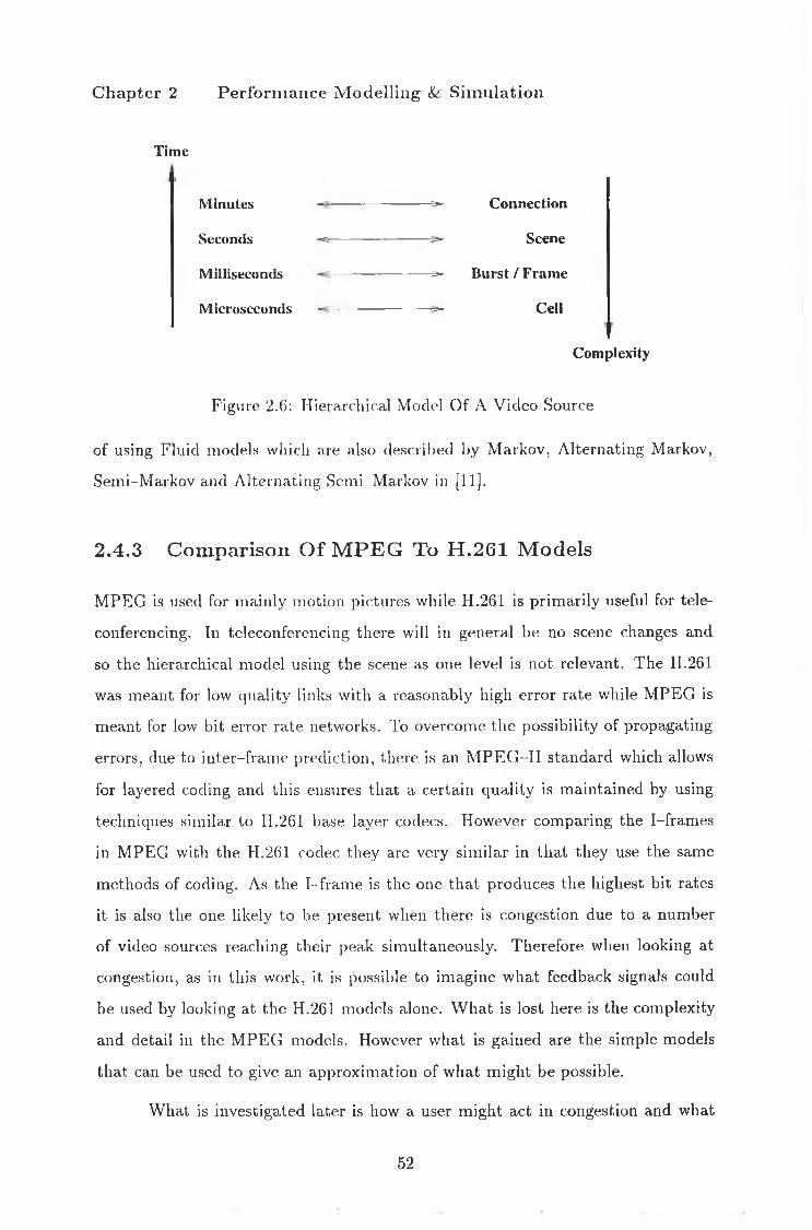
C h a p ter 2 P e r fo r m a n c e M o d e l l in g &; S im u la t io n
T im e
-5*- Connection
-==- Scene
•s*- B u r s t/ F r a m e
— Cell
Com plexity
Figure 2.6: Hierarchical Model Of A Video Source
of using Fluid models which are also described by Markov, A lternating Markov, Semi-Markov and A lternating Semi-Markov in [11].
2.4.3 C om parison O f M P E G To H .26 1 M od elsM PEG is used for m ainly motion pictures while H.261 is prim arily useful for teleconferencing. In teleconferencing there will in general be no scene changes and so the hierarchical model using the scene as one level is not relevant. The H.261 was meant for low quality links with a reasonably high error ra te while M PEG is meant for low bit error ra te networks. To overcome the possibility of propagating errors, due to in te r-fram e prediction, there is an M P E G -I I s tandard which allows for layered coding and this ensures tha t a certain quality is m aintained by using techniques similar to H.261 base layer codecs. However comparing the I-frames in M PEG with the H.261 codec they are very similar in th a t they use the same methods of coding. As the I-fram e is the one th a t produces the highest bit rates it is also the one likely to be present when there is congestion due to a num ber of video sources reaching their peak simultaneously. Therefore when looking at congestion, as in this work, it is possible to imagine w hat feedback signals could be used by looking at the H.261 models alone. W h a t is lost here is the complexity and detail in the M PEG models. However what is gained are the simple models th a t can be used to give an approxim ation of w hat m ight be possible.
W hat is investigated later is how a user m ight act in congestion and what
M inutes
Seconds -e-
M illiseconds
M icroseconds
52
C h a p ter 2 P e r fo r m a n c e M o d e l l in g &; S im u la t io n
use would there he of a feedback signal from the network indicating congestion. It might be possible in the fu ture for a video user to use a congestion signal from the network to lower the bit ra te by increasing the quantisation step used in the coding algorithm, or possibly to reduce the num ber of frames transm itted per second. For M PEG it would also be possible to increase the num ber of P -fram es and B-frames, bu t if the congestion is on the sub-fram e level then these m ethods would not really be useful as they would be too slow. Therefore it is likely tha t similar congestion avoidance techniques are possible for both the H.261 user and the M PE G user.
2.5 S im ulation TechniquesAfter models have been designed by normal modelling techniques there is then a choice of m ethods to gain insight in to the system and gain results from it through the model. It may be possible to have an analytical solution to the model bu t in a lot of cases this is not the case. The types of models th a t are dealt with here tend not to give analytical solutions in the detail th a t is required. This is mainly due to the fact th a t the system does not reduce to a product form solution, nor is it close to one. This is due to many factors but two of the m ain ones are th a t there are passive resources and there are priority schemes being used. There is also the problem th a t in the models there are em bedded heuristic algorithms. W hen it is not possible to get an analytical solution com puter simulation is an alternative. However there should be some crude analytical checks on the results from the simulations against the real system. The models th a t are designed are not static models bu t vary with time and so this fu rther complicates the analytical methods.
While modelling and simulation is a slightly indirect m ethod of studying the behaviour of systems it is sometimes a necessity when other alternatives such as observation or analysis are unavailable to us. In most cases com puter modelling and simulation is the only way of evaluating new networks and control m ethods which are only at the design stage. The simulation is based on a stochastic model and there is the issue of how long should the model run before there is consistancy
53

C h a p ter 2 P er fo rm a n ce M o d e l l in g & S im u la t io n
with the conceptual model. There are problems with simulation not alone in terms of verification but also due to the limits of com puting power available. Most of the simulation models will have problems relating to speed and m em ory of the com puting platform.
2 .5 .1 S E S / w o r k b e n c hT he simulation tool used to model the sources and the network is a commercial d iscrete-event simulator railed SES /workbench. [88]. Although a commercial package is slower to simulate in running tim e than raw C code, the t im e to get a model working is reduced considerably. It was felt tha t a lot more t im e would be saved by using a commercial package where models can be produced quickly even though the run time would be reduced. Even with raw C code it would be necessary to speed up the simulation tim e and this is easier to achieve using a package where m any methods can be tried out. SES /workbench, is used for software, hardw are and systems design. I t ’s use is not limited to com munication applications and it has been used extensively for non-engineering applications. SES /workbench consists of three modules, SES /design, SES / s i m and SES /scope.
SES /design is a graphical interface module th a t is used to specify the model. It can be used under an X-windows system which is what was used in this work. This graphical interface allows the building and designing of the models in a visual way and so eases the task of creating systems. An SES/ workbench model is a hierarchy of submodels where each submodel is a directed graph with nodes and links. There are predefined nodes available with the package and these include resource management, transaction flow control, submodel m anagem ent and some other types of nodes. The nodes can be used as is or it is possible to redefine them to have another configuration. A screen dum p of the 20 available nodes is shown in Figure 2.7.
The code behind the nodes is available to be altered. It is possible to write the SES simulation language called SES / s i m or to use C. W hen a model is built by SES /design then the o u tp u t of tha t will be a graphical model tha t
54

C h a p ter 2 P e r fo r m a n c e M o d e l l in g & S im u la t io n
P/<-|*?sinn 2.1 Module: nodesInd^yl Whar | Hr>w 1
Resource Management Nodes
■*1 0 *Service Delay
/ \Resource
Allocate Release Create
Destroy Block set
Submodel Management Nodes
E >>** HEnter Call
OD>2 - IReference Return
Transaction Flow Control Nodes
E > ~EESink
<1Source
Join Split
/
Fork
Loop
-»• >Interrupt Resume Branch
Miscellaneous Nodes
>1 b E MUser Declaration
Figure 2.7: S E S /design’s G raphical Interface
can be translated into a SES / s i m file. SES j s im is built upon the C program ming language. All SES / workbench files are transla ted into C before being translated into executable files. SES / s i m is similar to C and the expressions are the same in the two of them . Many declarations, expressions and sta tem ents are also the same, and even a function called “m ain” is needed to simulate a model. Because SES / s im is a superset of C it allows the user to gain access to a wealth of da ta underlying the model through a predefined set of variables, pointers, macros and run tim e library calls.
There are predefined probability functions contained in SES/ workbench, which include Poisson, geometric, binomial, Erlang, exponential, hyper-exponentia l, gam ma, normal, uniform and triangular distributions. Apart from these it is also possible to define a probability function empirically. T he probability functions either re turn an integer or a floating point num ber depending on the distribution
55

C h a p ter 2 P e rfo r m a n c e M o d e l l in g &: S im u la t io n
used. Ali of the probability functions and all the probabilistic modelling th a t is done in SES/ workbench uses random num ber generators. For random num ber generators there are a num ber of predefined ones as well as the possibility of defining one.
The predefined num ber generators include a pre-set linear congruential algorithm, a generic linear congruential algorithm and a card-shuffle algorithm. The pre-set predefined linear congruential random num ber generator is the default one and the one used for the work in this thesis. This is based on the following algorithm from [41] :
r / „ s ta tes ta te = { (a s ta te + b) mod ??i } ; rv — -------m
where rv is the random variable produced, ‘s ta te ’ is the s ta te of the algorithm which is initialised to the seed value, a = 1664525, b = 1664525 and m = 232. T he ‘s ta te ’ is initialised with the seed value of 314159, which can be altered in the code. One of the advantages in using this algorithm is tha t for a 32 bit machine, the algorithm is optimised and is quick to run. This is mainly because the m odulus function is done autom atically by having only 32 bit precision available. A nother advantage of using the predefined, p re-se t random num ber generator, is tha t for different runs of the program the same sequence of random num bers will appear. This means tha t the model will perform the same, unless the seed or random num ber stream is changed, and this allows for debugging of the model by going to a particu lar part of the run tim e, again and again, and getting the same results. It is possible to change the seed and the random num ber generator while the simulation is running, and it is possible to create many instances of the random variables. For most of the following work the random num ber generator used is the predefined, p re -se t random num ber generator.
The final module in SES /workbench is the running of the model and the examination of the results. This is available with the use of the SES /scope. SES /scope allows the user to anim ate the model and so to visualise exactly w hat is occurring in the simulation. A typical ou tpu t of the SES /scope is shown in Figure 2.8. It is possible to m ake an executable th a t is not an im atable and this will run quicker
56

C h ap ter 2 P e rfo r m a n c e M o d e l l in g &z S im u la t io n
than an executable tha t is anim atable. For the debugging stage it is useful to have the animation. SES /scope allows interaction with the model as it is running as well as controlling some param eters of the model. T he operation of SES /scope is through a graphical interface th a t is similar to S E S /design. It is possible to get detailed information from the model on the screen and to dum p this to a file. Apart from statistics th a t are collected from the SES /design it is also possible to pu t inspectors on any variable in SES /scope. W hen a variable has an inspector a ttached then a graph of the performance is possible as is shown in Figure 2.8.
SEf'/rl^i-. i inn .1,1
q u e u e _ s o u r c e• 5 © *
m _jn_l_queue-EE
q u e u e _ s i n k
m number_J.n_queue: p o p u la t io n :C u rre n t I f M10
/ uv " J W y ^
o’ 10 Time 0 . 21 '
0 n umber _i n . q u e u e l § f r a lS t a t i s t i c p o p u 1 a t i o nC a t e g o r y A l lC u r r e n t 4Min 0Mean 5 .1 7 7 3 1Max 9V a r i a n c e 4 .5 4 2 3 1C o u n t N/A
ITOI 0^479 jJHfS to p >1 T r a n s
I #i i ■ "a
S c o p e S e t t l n q sT r a f f i c C o n t r o l B No Log F i l e
( 4 6 , p a c k e t , U, NULL} @ 0*1479 c r e a t e d a t n o d e m_m _l. q u e u e _ s o u r c e{46, p a c k e t , 0 , NULL) @ 0 . 1 4 7 9 a t m_m_l . q u e u e _ s o u r c e s c h e d u l e d t o b e a c t j ^ ^( 4 6 , p a c k e t , 0 , NULL) @ 0 . 1 4 7 9 a c t i v a t e d a t m _m _l . q u e u e _ s o u r c e
n u m b e r _ o f _ « r r i v anum ber _ o f . . d e p a r t
n umber _ i n _queu(S) n umbe r .. I n _ g u e u e :
Figure 2.8: SES / s c o p e ’s Graphical O u tpu t
The simulation execution p latform was a cluster of Sparc-10 workstations. The workstation running UNIX can support m any sessions of SES at the same time. It is possible to remotely run SES from any com puter th a t supports X-windows emulation. There are a num ber of m ethods of achieving tha t . T he popular m ethod is by running a UNIX operating systems and even on a PC this is possible by running “LINUX” . If this option is not available then it is possible to have an X-window em ulator like “X -W in ” . This allows SES to be controlled from any PC with a connection to the internet.
57

C h a p ter 2 P e r fo r m a n c e M o d e l l in g &c S im u la t io n
2.5 .2 Source S im ulation M o d el D es ig n2.5.2.1 Voice Source Sim ulation M odel Design
The voice model produced by SES /workbench is on the cell level, so th a t each cell time a decision is taken on whether or not to produce a burst of cells. The transmission line is thus divided into cell times, and tha t is the smallest tim e unit considered. The size of the burst is the num ber of cells tha t will be tran sm itted and is chosen from the geometric distribution . W ithin the burst the cells are not back- to-back but ra ther at the cell ra te given by the voice source while on. After the burst the silence interval is chosen and no cells are produced. W hen the source does not produce a cell then a time is chosen from the hyper-exponentia l d istribution and no cells are produced in tha t interval but a cell will be produced in the next interval. It is possible using this model to find out how many cells will be produced in a fixed tim e interval and to find the num ber tha t will be produced in the interval after tha t as well. This allows for a speed-up of the simulation when there is no longer a need for cell-by-cell simulation.
2.5.2.2 One Layer V ideo Source Sim ulation M odel Design
Simulating the one layer model is sum m arised in Figure 2.9 1. T he basic t im e unit is a frame tim e or 0.04 seconds, which emulates a codec running at 25 frames per second. The b irth death process makes the model much simpler because instead of having 64 arcs connecting all the states to each o ther there are only 16 arcs. The transition m atrix for this b ir tl i-dea th process was shown in Figure reftrans.
Executing the model produces a num ber of ATM cells based on the range of bit rates th a t a particular s ta te represents. As shown in Figure 2.9 the model can enter a new sta te at a ra te of 25 per second. T he probability of a transition between states is determ ined by the normalised transition m atrix. On entering a s ta te the model produces a num ber of ATM cells. T he num ber produced depends on the sta te being entered and is uniformly d is tr ibu ted across the range of a tta inab le values in
lrThe bucket here corresponds to the state of the Markov-Chain and specifies the allowable bit rates, or frame sizes, for that time period.
58

C h a p te r 2 P er fo rm a n ce M o d e l l in g &c S im u la t io n
Iterate every 1/25 sec1
( Enter A N ew B ucke t)
This sim ulates the codec running at
25 Fram es per second.
Bucket
lb (kb/s) ub (kb/s)lb = I ew er bound ub= upper bound
\ /Produce A Num ber Of
O f A TM Data Cellscoll 1
x=4fl bytes (384 bits)
- a x k -. ... [ call h |-cont
Attach Header To Cells ( + 5 Bytes ) &
Tx Cells & ATM Line Hate
Figure 2.9: Process For Simulating The One Layer Codec
th a t state . Since the empirical da ta set for the coded video sequence presented the d a ta on a bit ra te per second format for each frame it was necessary to convert this d a ta to ATM cells. If the cell load was not filled with video information, the cell was sent anyway as it was tim e critical. This is similar to rounding up the integer values of the num ber of cells. T he AAL 3 /4 was used to show a possible im plem entation with 44 bytes of information per cell. ATM cells are generated equally spaced in tim e over the. frame duration , which is using source shaping.
2.5 .2 .3 Two Layer V ideo Source Sim ulation M odel D esign
Im plementing the two layer model was quite similar to the one layer model. In this case, however there is not a s ta te diagram but ra the r a single s ta te for the base layer and a s ta te for the enhancement layer. The base layer produces a num ber of cells each fram e tim e, where the num ber of cells produced is chosen uniformly between the limits of the base layer. The enhancem ent layer uses a hyper-exponentia l distribution, and so a num ber of cells is chosen from th a t each frame time. As
59

C h a p ter 2 P e r fo r m a n c e M o d e l l in g &: S im u la t io n
before the rounding of the continuous variables to the integer num ber of cells is up, so tha t cells th a t are not completely filled with video information are transm itted. Both the enhancem ent and base layers run at the same t im e combining to form the two layer codec output.
2 .5 .2 .4 D a t a S o u rc e S im u l a t i o n M o d e l D e s ig n
The data model produced by SES /workbench is th a t of a file transfer application. There are two param eters of interest, the file, size and the num ber of files to be transferred. T he assumption is th a t a num ber of file transfers is possible simultaneously. The file size has been chosen from a probability distribution tha t is empirically based. This d istribution was chosen from a sample of about 200 files on a PC [78], which varied in size from small tex t files to large executables. Both the ra te of file transfer and the num ber of files to be transferred simultaneously are based on probability distributions. These can be changed bu t are currently based on uniform distributions.
2.5.3 Source Sim ulation M o d el V alidationIt is generally felt th a t there are three steps in deciding if a simulation is an accurate representation of the actual systems considered [26, 33, 44], T he first step is to v e r i fy the model, tha t is to make sure th a t the com puter simulation acts as it is intended to against the conceptual model th a t has been designed. This generally involves debugging the code and can be aided by using modules of code rather than a large program. It also includes trying the systems under a num ber of input param eters. The software used [88] also allows the use of traces which are a powerful m ethod of checking on the s ta te of the system. This was used extensively and was checked with hand calculations of the models to check the simulation. It was also possible to anim ate the systems using SES /scope and this provided a visual m ethod of verifying the models. Another m ethod was to check against certain conditions occurring and this was also possible to do with SES /scope. Once the model produced is verified then the com puter simulation portrays the intended
60

C h a p ter 2 P e r fo r m a n c e M o d e l l in g &l S im u la t io n
system model. The next step is to v a l i d a t e the model so th a t the conceptual model can be considered to be accurately representing the real system. This validation is done by comparing the models to what is generally accepted as the real system, or in the case here the models represented in the literature. T he real system for this exercise can be thought of as the previous results and characteristics of the sources. The final step in the simulation is to ensure tha t the models are c r e d i b l e which is to see if the simulation is accepted as being accurate and useful. For the purpose of this research this would am ount to publication of the simulation details, models and methods. The relationship of these steps can be seen in Figure 2.10.
Validation
Figure 2.10: Relationship Between Verification, Validation and Credibility for Simulation Models
The voice model was verified and validated against the model of voice tha t is commonly used in the published literature [12, 29, 64]. T he main check was to see if the m ean ‘on’ t im e and ‘off’ time were similar to the models published. The d a ta model was verified bu t validation of this model is difficult as there is not a s tandard model. Again the check was to see if the model was accurate with respect to the conceptual model. T he validation of the model will be considered in the context of the overall modelling as the actual characteristics of the d a ta model should not affect the results of the simulations. The video models were verified and then validated by comparison to the characteristics of the d a ta th a t was captured from H.261 type algorithms. A first approach was taken by visually comparing the PD Fs of the empirical d a ta with those of the models. However due to the cell s truc tu re of the models there is a discrete effect on the PDF, and so visual
61

C h a p te r 2 P er fo rm a n ce M o d e l l in g Sz S im u la t io n
comparison was difficult. It was noted however tha t some edge effects were taking place at the boundaries of the states where a certain cell size was being favourably trea ted by being in two states. This was duly eliminated from the model. The basic measurements tha t were observed were the m om ents of the models and these are compared in Table 2.4 for the one layer model.
Table 2.4: Validation Of T he One Layer Codec Model
Param eter Empirical ModelMean ( in b /s ) 216 E + 3 223 E + 3Second Moment 2.08E+10 2.22E+10Root of Second M oment 144 E +3 149 E + 3T hird Moment 1.9 E +15 2.2 E +15Cubic Root of Third M om ent 124 E + 3 130 E + 3
These results show th a t statistically the model is producing similar m om ents to the empirical data. To validate the model further, the correlation functions should be taken and compared for the model and the data . For the two layer model the mean bit ra te produced is chosen to be identical to the empirical d a ta and the standard deviation is similarly chosen.
2.6 H ig h -S p e ed S im u lation P ro b lem sAs mentioned previously there are a num ber of problems associated with simulation of high-speed networks. As the bit ra te increases then the num ber of events per second also increases at the bit level. If the bit level was to be sim ulated then the slow-down of the simulation would be linear with the increased bit rate. However most of the work presented here is simulation at the packet or cell level. If the packet size increased according to the speed of the network then there would be no real increase in the simulation tim e as the cell ra te would remain the same going from low-speed networks to high-speed ones. However with ATM not only has the bit ra te increased but the cell size has got quite a lot smaller com pared to the
62
C h a p te r 2 P er fo rm a n ce M o d e l l in g & S im u la t io n
previous d a ta networks. For example E thernet frames are about 1500 bytes while ATM cells are only 53 bytes, and the bit ra te on E therne t is 10 M b/s compared to 155 M b/s on ATM. This gives an overall increase in simulation tim e from Ethernet to ATM of which is over 400 if the sam e m ethods and complexity of models isassumed. This decrease in cell size is counter intuitive as the higher speed networks have b e t te r error characteristics than the slower networks, and so larger packets are more efficient and also possible. However for ATM it is expected tha t the error control will be en d -to -end and not hop-by-hop . There is also the consideration of the real tim e services, and especially the low bit ra te ones like voice, which could not be carried in large packets due to high packetisation delays.
An indication of the efficiency of the simulation can be expressed in terms of the speed-up or slow-down factor. The speed-up factor is the num ber of seconds tha t can be simulated of the real system for one second of the processor time. The slow-down factor is the num ber of seconds of the C PU tim e needed to simulate one second of the real system. Using a Sun Sparc-10 with SES / workbench the speed of simulation can be es tim ated to be about 4,000 events per second [61]. This is comparable to other simulators th a t are discrete event based like O p-net. If the bit level was to be simulated and one bit were one event, an over simplistic assumption, then the slow-down factor would be nearly 40,000 for a 155 M b/s ATM link. This would mean than one second of the real system would take about 11 hours to simulate. However if cell level simulation is done then the slow-down factor is reduced to about 100. W hile the aim of the simulation would be to get the simulation to run as fast as the real system there is still room for improvement. Also in any reasonable size model there will be about 20-100 events per cell, so speed-up techniques of the order of 1,000 or so are still needed.
Even if the speed of simulation were not im portan t, there are other problems with the memory of the com puting platform. Again typical models allocate about 4 kBytes of memory to each basic simulation unit, be it cell or bit. Assuming tha t the simulation is at the cell level and th a t the ATM bit ra te is 155 M b/s, or 365,566 cells per second, and if the delay in the system were to be 0.02 seconds then the com puter would have to track about 7311 basic simulation units, and as each of
63

C h a p te r 2 P e rfo r m a n c e M o d e l l in g & S im u la t io n
them needs 4 kBytes of memory, the com puter needs to have about 30 Mbytes of memory. A typical Sun Sparc-10 has about 28 M bytes and while it is possible to increase this it costs more and does not really solve the problem. While in a lot of applications delays of this order would not be encountered there are a num ber of areas investigated in this work where they are. One is the long delay satellite links, where round-tr ip delays are of the order of 0.5 seconds. A second example is when there are m ultiple sources, and typical num bers of sources in a 155 M b/s single link could be of the order of 100. Therefore the m ax im um delay is now only allowed to be 0.2 milliseconds. This only represents a buffer size of about 75 cells.
Therefore there is a need to examine a lte rnative m ethods to both speed up the simulation tim e and reduce the amount of m em ory used in the simulation. There are a num ber of approxim ation techniques used in the lite ra ture [8 , 9, 26, 33, 44], and some of these are described below as they are used in the simulations.
2.6.1 D eco m p o sit io n M eth od sDecomposition is a m ethod of splitting the model into smaller models and then solving each independently. When this is done the results can be aggregated to form an approximate, solution. W hat is nice about decomposition is th a t for a num ber of communication systems the decomposition gives exact results [33]. If a model can be m ade to be in a product form then the solution is exact and this m ethod is generally called the llow-equivalence method. W hen the model is almost product form then the decomposition produces good approxim ations. W h at is surprising is th a t even for models which clearly violate product form criteria the results can be good. W hat makes the models here non-product form is th a t there are passive resources which inhibit the product form solution. T he m ost common form of passive resource th a t is here is the window size th a t is used for retransmission schemes. If this could be ignored then this problem would be removed. There is also another problem in th a t there are a num ber of heuristics th a t are em bedded in the model, as well as a num ber of priority schemes and these complicate the solution. However use is still m ade of the decomposition m ethod.
64
C h a p ter 2 P e r fo r m a n c e M o d e l l in g &; S im u la t io n
When using some approxim ation m ethods it is difficult to produce error bounds on the results due to the na tu re of the approxim ation. This can be particularly true for ad-hoc m ethods and intuition is appealed to for the justification and acceptance. While decomposition is generally applied to states of a system it can also be applied to tim e periods as well. In tim e decomposition what is achieved is to split the model into m any pieces, and each one is valid for a period of time. T he more detailed model takes more tim e to run, bu t this m ay be only needed for a small fraction of the t im e and m any orders of m agnitude can be gained by this m ethod [55, 58, 61].
2.6 .2 C e ll-R a te M eth o d sA cell-rate m ethod considers a burst or group of cells to be the basic simulation unit ra ther than the cell [8 , 18]. This allows a speed -up of the simulation as the num ber of units to be simulated has dropped. During a t im e period while the burst is active the inter-arrival t im e of the cells is constant and what changes in the simulation is the tim e a burst is active and the cell ra te while in a burst. Because the inter-arrival tim e of the cells is constant in a burst it is possible to solve the multiplexing of sources in a buffer by considering the rates ra ther than the cells. A typical tim e period of interest might be as shown in Figure 2.11 and it can be seen tha t the speed-up can be considerable, for exam ple it could be many orders of magnitude.
For this m ethod to produce good results what is needed is a large num ber of cells to be represented by a single event or burst. This usually means tha t either : 1 the burst has a long duration and the cell ra te can be small or else ; 2 if the burst length is short in t im e then the cell ra te of the source should be high. For example the gain in using this m ethod for voice would not give good results as the bursts are short and the bit ra te is low, and hence the cell ra te , is low also. However for da ta file transfer this can improve the simulation tim e considerably. W h a t can be seen is tha t the design of the models should be m ade with the approxim ation technique in mind to get good results.
65

C h a p te r 2 P e r fo r m a n c e M o d e l l in g &c S im u la t io n
cells/sec
600
400
200event 1 event 2 event 3 event 4
seconds
Figure 2 .11: Events in a Cell Rate System
2 .6 .3 S t e p -B y - S te p M eth o d sA proposed approxim ation m ethod is to break the possible times of simulation up into different parts and then to develop different models for each period. This type of simulation approxim ation is called a S tep -by -S tep m ethod [9, 17]. W hile there can be many different models, it is sometimes possible to gain a considerable speed-up with just two models. The simulation would normally consist of one detailed model and one coarse model tha t can run quickly. T he simulation runs with the coarse model until the detail in the detailed model is required and then the simulation steps into th a t model. Therefore it is only when the required detail is needed tha t the detailed model is used.
An example of this m ight be the loss from a finite buffer. A tim e interval could be chosen th a t is small enough so tha t not a lot of cells can arrive in one interval, and therefore it is possible to predict when cell loss is going to occur, bu t long enough to speed up the simulation. W hile the buffer is em pty it is possible to step along in tim e and not to consider how the individual cells arrive. However if the buffer fills to a certain stage then the model is changed into the detailed model and m aybe go at the cell t im e until the buffer empties and then swap back to the coarse model. Therefore at the end of each tim e interval the decision is m ade whether to stay in the coarse model or to change to the detailed model. This t im e
66

C h a p te r 2 P erfo rm a n ce M o d e l l in g &; S im u la t io n
interval of course can change dynamically during the simulation. The tim e interval will decide on the accuracy of the simulation and the speed and there is the normal trade off between the two tha t the more accurate the longer the simulation tim e is needed and the shorter tim e spent in the coarse model, and the more tim e in the detailed model.
2.7 D iscu ssionT he models presented in this C hap ter detail the modelling design and simulation techniques tha t are used in the rest of this report. An introduction to modelling was given along with detail about modelling of ATM networks. Various source models were presented and validated from the design to the simulation model. T he platform where, the simulations were executed was discussed as well as the simulation package. Various problems were pointed ou t in connection with ATM networks and some approxim ate solution to these has been given. T he whole process of modelling and simulation is circular in n a tu re with many iterations of the design, simulation, analysis validation and approxim ations. All the individual stages depend considerably on each other so none can be trea ted in isolation.
67

Chapter 3
Cell Level R esource A llocation
3.1 In trod u ctionThis chapter deals with cell level resource allocation issues. Of concern here is the structure of the ATM cell and how there is adap ta tion of the ATM to higher level services. There are problems encountered when using ATM in non-fiber optic systems and we investigate those lim itations when using ATM over a satellite link. Again at the cell level the use of traffic controllers poses problems for using resource allocation methods due to the unclear position of the worst case traffic tha t can be allowed through the controllers.
It is shown here how it might be possible to adap t ATM to satellite links. ATM is a h igh-speed protocol designed with optic fiber as the intended transmission medium and therefore several problems arise when satellite channels are used. A solution is proposed here for the error control mechanisms to adapt to the satellite channel by moving the error recovery and detection to a higher layer of the ATM. The error recovery tha t is proposed here is to use the ability of the ATM to determ ine the service of the retransmission and to base recovery on tha t service. The simulation results here show th a t not only is there an increase in the raw data throughput for satellite channels to alm ost the theoretical limit, bu t there is an improvement in the d a ta transfer efficiency of the ATM by 7.5%. T he results also show th a t it is possible to guarantee d a ta services with no loss of d a ta under certain conditions.
68

C h a p ter 3 C ell L eve l R eso u rc e A llo c a t io n
ATM networks allow for the input traffic from users to vary both from one connection to another and within the connection. ATM specifies a m ethod for controlling the traffic, flow across the user network interface ( UNI ). This involves each user negotiating connection param eters with the network. Once these param eters have been decided then a contract is made between the user and network. T he network must then enforce the contract in order to guarantee performance and quality of service to other users. W hat is of interest to the network is, given a particular set of users and contracts, what is the worst traffic th a t the users could input to the network while still abiding by their contracts? This type of input traffic would be called the worst case traffic as it would produce the lowest performance in the network. The reason why this is of importance is th a t for network performance it is im portan t to have the worst case traffic inputs. Furtherm ore, it is im portan t for the network traffic controller to know the possible worst case traffic so th a t it can assign resources accordingly.
The standards organisations have decided 011 an initial contract type for connection admission [4] and this is called the generic cell ra te algorithm. This is not ruling out the possibility of other types of contract descriptions being implemented in the future, but allows development of systems at this stage. W hat is needed now is to decide what type of traffic can still pass these contracts and produce the worst or lowest network performance. This problem has been studied in the literature [23, 83, 84]. Some theoretical background is given here, to explain some of the results in the literature, and a further look is taken at some examples of types of worst case traffic sources. It is shown here for the two most common types, the greedy on-off and the three s ta te source, th a t depending on the situation either can be worse [24, 62]. This would imply th a t neither of these types is generally the worst case traffic type as has been considered for the last num ber of years.
Ill the first par t of this chapter the problem of using ATM over satellite is addressed, while in the second part the worst type traffic tha t can pass the generic cell rate algorithm is investigated.
1. In Section 3.2 the reasons for using ATM over satellite are m otivated as well as
69
1
give a detailed description of the deep space network. T he deep space network is used by .JPL for com municating with u n -m an n ed space missions. Some problems with satellite ATM transmission are also exam ined. In Section 3.3 there is a description of the modelling of the satellite link and consideration is given to the decomposition m ethods used for the simulation. In Section 3.4 the issue of adapting the ATM to the services is considered. T h e problem with current adapta tion m ethods is pointed out as well as a proposed solution and some notes on the ability of ATM to be service selective in terms of retransmission schemes. Section 3.5 deals with the simulation of the satellite link and the results tha t are gained from the simulation. There is also some detail on the validation and theoretical comparison of the results and the design of the adapta tion scheme proposed.
2. Here the worst type traffic, th a t can pass the generic cell ra te algorithm is investigated. In Section 3.6 the cell level congestion and control area is explored and some detail is given about the s tandards approach and definition of congestion and usage param ete r control. T he leaky bucket is described as it is the s tandard usage param eter control. In Section 3.7 the issues tha t are dealt with here are introduced and a description of two worst case traffic types is given. There is also some discussion on the suitability of finite and infinite buffers in the analysis and the continuous and discrete variables. In Section 3.8 the new analysis used is presented for dealing with worst case cell traffic. Some supporting examples are then presented in Section 3.9 and both the case of a fast and slow server is analysed.
Finally there is discussion of the chapter in Section 3.10
3.2 M otiva tion For A T M O ver S a te lliteW hile ATM has been proposed for high speed services, at rates of 155 M b/s and622 M b/s, there is increasing interest in ATM at lower rates [14], such as 1.544 M b/s( T1 ). The interest of using ATM at low bit rates is s tim ula ted by two m ain factors :
C h a p ter 3 C ell L eve l R e so u rc e A l lo c a t io n
70
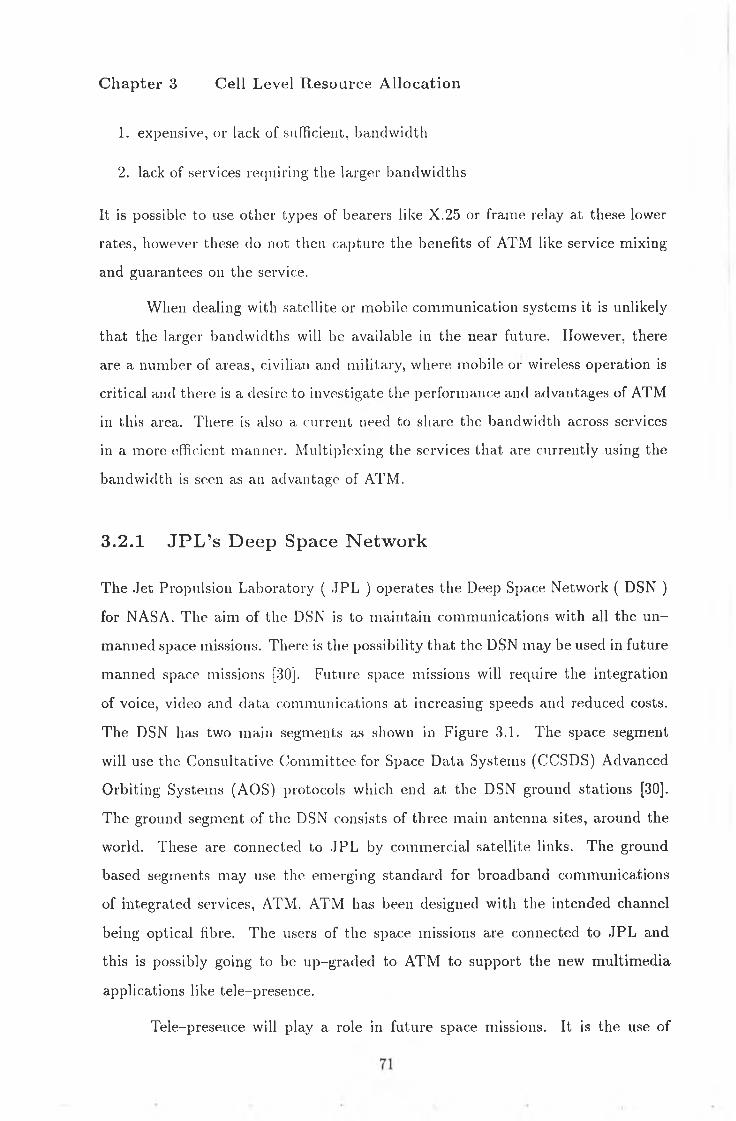
C h a p ter 3 C ell L eve l R e so u r c e A llo c a t io n
1 . expensive, or lack of sufficient, bandw idth
2 . lack of services requiring the larger bandwidths
It is possible to use other types of bearers like X.25 or frame relay at these lower rates, however these do not then capture the benefits of ATM like service mixing and guarantees on the service.
When dealing with satellite or mobile com munication systems it is unlikely th a t the larger bandwidths will be available in the near future. However, there are a num ber of areas, civilian and military, where mobile or wireless operation is critical and there is a desire to investigate the performance and advantages of ATM in this area. There is also a current need to share the bandwidth across services in a more efficient manner. M ultiplexing the services th a t are currently using the bandw idth is seen as an advantage of ATM.
3.2.1 J P L ’s D eep Space N etw orkThe Je t Propulsion Laboratory ( JP L ) operates the Deep Space Network ( DSN ) for NASA. T he aim of the DSN is to m ain ta in communications with all the unm anned space missions. There is the possibility th a t the DSN may be used in future manned space missions [30]. Fu ture space missions will require the integration of voice, video and d a ta communications a t increasing speeds and reduced costs. The DSN has two main segments as shown in Figure 3.1. The space segment will use the Consultative C om m ittee for Space D ata Systems (CCSDS) Advanced Orbiting Systems (AOS) protocols which end at the DSN ground stations [30], The ground segment of the DSN consists of three main antenna sites, around the world. These are connected to JP L by commercial satellite links. T he ground based segments m ay use the emerging s tandard for broadband communications of integrated services, ATM. ATM has been designed with the intended channel being optical fibre. The users of the space missions are connected to JP L and this is possibly going to be up-graded to ATM to support the new m ultim edia applications like tele-presenc.e.
Tele-presence will play a role in fu ture space missions. It is the use of

C h a p ter 3 C ell L evel R eso u rce A l lo c a t io n
Space Segment
Spain
Ground Segment
NASA Backbone
Figure 3.1: Deep Space Network
communications to provide a remote projection of hum an presence, for instance this can be done with robotic rovers remotely piloted by ea rth based scientists. Robotic rovers require stereo vision using low ra te compressed images. Therefore tele-presence m ethods require transmission of in tegrated video and data . Future m anned missions will require, integrated voice, data , and video communications systems [31, 32]. Cost minimisation requires the establishm ent of standardised communications techniques tha t may support these services.
The bit rates being used on the commercial satellite links in the ground segm ent are generally T l or less. The services th a t use these links vary from com m and files for spacecraft and ground distribution of telemetry, to voice communications among operators and test data. There is also the fu ture possibility of using these links for digital video. The accuracy of the d a ta from and to spacecraft is critical while o ther d a ta and voice to the other earth sites m ay not be as im portan t. At present there is no autom atic m ethod of differentiating between the different services th a t use the network.
72

C h a p ter 3 C ell L evel R e so u rc e A l lo c a t io n
3.2.2 P rob lem s U sin g Satellite Links For A T MBecause ATM has been designed with optic, fiber as the expected transmission medium this means th a t the expected errors will be produced by Gaussian noise and will introduce random geometrically d is tr ibu ted b it errors. T he bit error probability is denoted by pb and can be expected to be approxim ately pb = 1 0 -10 for fiber optic cable. ATM cells are 53 bytes long, or 424 bits, and so it is possible to calculate the probability for cell error. It is possible to further calculate how many of these errored cells have, ju s t a single bit in error, and then work out what the probability of more than a single bit in error is.
^ r c.ell in e r ro r ̂ 7;f>)= 4.24 10~8
^ s i n g l e b i t in e rro r — ^24 Pb ^ ~ Pb)= 4.2399 10" 8
424
4 2 3
^>1more than single bit in error { ̂ ^ f̂>) }\4 2 3- { 424 P6 ( l - Pbr )
Using an expansion for the (1 — pb)n te rm the following equations are got, and a bound on the error on the. result from the series expansion because of the alternating series can be found :
*̂rmore than single bit in error= { ! - ( ! - 424 pb + - 0 ( p t ) }
- {424 pb ( 1 — 423 pb + O(pl) ) }
= {424 Pb - p2b + 0 ( p 3b) }2 i- {424 pb - 424 -423 p\ + 0 ( p 3b) }
= 89676 p2b - 0 ( p 3b) = 8.967 1(T16 « lO" 15
73

C h a p ter 3 C ell Level R e so u rc e A llo c a t io n
W h at can be seen is tha t nearly all the errors will be single bit errors or less than 1 in 107 errors will be more th a t a single bit error. In fact for a 155 Mbps system, more than a single bit error would onlt occur every 80 years or so. Therefore error detection and single bit error correction will almost fully protect the data.
In satellite links bursty errors are common as will be seen in Sub-Section 3.3.2. These bursts may be a result of Gaussian noise, but ra ther than producing randomly distributed bit errors they produce a large group of bit errors due possibly to the coding of the channel. It is also possible th a t degraded performance m ay occur on the link causing increased bit errors which may destroy the link for a fraction of a second or more. On top of these bursty errors there is also background Gaussian noise which might produce error of the order of 10-6 . This introduces a different type of error distribution to what can be expected from optic fiber cables. The probability of having more than a single bit error, can also be calculated :
^ rmore than single b it in error= { 1 - (1 - Pby 24 } - { 424 Pb (1 - Pb) 423 }
= 89676 p2b - O(pl) = 8.967 1 0 " 8 « 10“ 7
This would mean tha t the same 155 Mbps system would have more than a single bit errored cell every 30 seconds or so and 1 in about 4000 errors will be more than single bit errors. Therefore single bit error correction is not likely to protect the data. The probability for loss of the d a ta and the header of an ATM cell is shown in Figure 3.2 versus the bit error probability for Gaussian noise.
It is seen tha t for optic fiber m edia there is about one cell lost every century for a 155 M b /s link whereas for satellite links the loss will be about one cell every minute. Therefore different error-detec.tion methods must be im plem ented when using ATM over satellites. If the errors were likely to be all bursty then it is possible to use the cell header to p ro tec t the d a ta and the incorrect cells could be discarded. For example if the bit error probability was 10- 7 b u t all the errors occurred in blocks of 400 bits, then when an error is got either one or two cells will be in error. The cell error probability is then less than 2 10- 7 which is b e tte r
74

C h a p te r 3 Cell Level R e so u rc e A llo c a t io n
Figure 3.2: Loss For 155 M b/s Link For Various Bit Error Rates ( B E R )
than optic fiber with pi> = 10- 9 . However with bo th bursty and random errors there have to be other schemes implemented to com bat the errors and to protect bo th the ATM cells and the d a ta th a t is contained within them . There are many schemes proposed to adapt ATM to non optic fiber environm ents [7] however these do not take into account the type of error found on the satellite links used by JPL. W ith any of the schemes proposed so far there is always the probability tha t the cell header m ay be correct and the d a ta contained within the cell is corrupted. It is assumed tha t there are some higher layer protocols, like T C P /IP , th a t look after these errors. However in the DSN this may not be the case.
Another problem in using ATM over satellite links is th a t the delay of the link is large and therefore there can be a large num ber of cells, or indeed higher layer d a ta units, outstanding on the link at any time. W hen designing the num bering scheme in ATM, and the adap ta tion layers, for fiber optic cables the delays are relatively small. This means tha t the num bering schemes in ATM m ay not be sufficiently large to allow the satellite link to operate in continuous transmission mode. This problem is called sequence num ber starvation [6] and can be overcome by either : 1 allocating more bits, and therefore more num bers, for the same cells or d a ta units; or 2 numbering larger d a ta units than before where the cells were
75

C h a p ter 3 C ell L eve l R e so u r c e A l lo c a t io n
num bered.
3.3 M easu rin g &: M o d ellin g A S a te llite LinkThe satellite link is characterised by the delay across the link and the bit ra te of the link. In this model the delay across the link is taken to be 270 milliseconds, and the bit ra te of the link is T l , or 1.544 M b/s . There is also the error due to incorrect decisions on the. bits a t the receiver. T here are m any models proposed to model this bit error and most are based on reasoning why the errors occur. R ather than take one of the predefined models or be involved in the actual coding and transmission schemes being used on the link, an empirical model based on actual test da ta taken from the DSN is used here. There is an am ount of d a ta tha t was collected from the DSN and the m ethod in which this was collected is described in Sub-Section 3.3.1 and then the actual d a ta is presented in Sub-Section 3.3.2. W hile looking at the d a ta it is im portan t to keep in m ind th a t the end result will be to perform simulations. There are problems in simulating long delay systems and so the modelling of the noise is critical.
3.3.1 E xp erim en ta l Test S e t—upThere was a study done on the DSN satellite links between the start of January 1992 and the. end of October 1992, a 10 m onth period [50]. This report examined the satellite links to produce results for both the circuit availability and also the circuit error characteristics. The only par t th a t is of concern here is the circuit error characteristics. The Ground Com munications Facility ( G CF ) at JP L consists of satellite links and the digital connections th a t connect the satellite links to the central site in Pasadena, CA. The unit of d a ta th a t is being used on these links is a NASCOM standard where the blocks of d a ta are 4800 bits in length [50]. T he links tha t are of concern to the report are the prim e and backup circuits which are :
76

C h a p ter 3 C ell L eve l R eso u rc e A llo c a t io n
• Prim e Circuits- Golclstone System 2, 1.544 Mbps, direct satellite- Canberra, 512 kbps, direct satellite- Madrid, 512 kbps, direct satellite
• Backup Circuits- Goldstone System 1 , 1.544 Mbps, direct satellite- Canberra, 64 kbps, undersea cable- Madrid, 56 kbps, terrestrial & satellite via GSFC
It is only the satellite links th a t are directly connected th a t are of concern, which are all the prim e circuits and the Goldstone backup circuit. 12 error ra te tests were conducted as par t of the study, and these results were reported on in the report. It was also possible to examine the receiving test set th a t was stored on electronic tape. Naturally the error rate tests were not carried out on the whole of the link capacity, as the links had to remain operational at all times. The error ra te tests are shown in Table 3.1.
The tests num bered 2, 3 and 8 , in Table 3.1, are not all satellite connections and so are not analysed here. In the tests num bered 5 and 6 , in Table 3.1, it was found out, after the tests were completed, tha t there was not enough transm itte r power being used and so these will not be analysed here either. So the tests tha t are further examined are 1 , 4, 7, 9, 1 0 , 1 1 , 1 2 . The error ra te tests th a t were carried out were one way tests where the d a ta being sent was generated and received at the far end by a “F irebird” test set. These test sets count the bit errors, block errors, blocks transm itted and other statistics. Every 10 m inutes the contents of the test set is available a t the output.
3.3 .2 E xp er im en ta l D a ta For Error D istr ib u tionT he experim ental d a ta used to model the error d istribution are from fractional T1 links, which vary in bit ra te from 56 k b /s to 224 k b /s and the tests were taken over a period from less than a day to about two days. T he results from the tests, tha t were described in Sub-Section 3.3.1, are summarised in Table 3.2.
77

C h a p ter 3 C ell L eve l R e so u r c e A llo c a t io n
Table 3.1: Error Rate Tests On T he G C F O f T he DSN
Test Link Bit ra te in kbps
Duration in hours
1 Canberra to JP L prime 56 412 Canberra to JP L backup 64 453 Madrid to JP L backup (via GSFC) 56 514 JPL to Goldstone prim e 56 445 Madrid to JP L prime 1 1 2 76 Madrid to JP L prime 56 527 Goldstone to JP L prime 224 178 JPL to Madrid backup (via GSFC) 56 519 JPL to Goldstone prime 224 10
10 JPL to Goldstone prime 224 24.511 Canberra to JP L prime 224 3512 JP L to M adrid prime 56 51
Table 3.2: Detailed Selected Error R.ate Tests
Testnum ber
Bit rate in kbps
Duration in hours
Blockstransm itted
Blockerrors
Biterrors
Bit Error R ate
1 56 41.28 1,728,990 0 0 0
4 56 43.7 1,835,213 16 3,151 3.58E-77 224 16.67 2,799,954 11 191 1.42E-89 224 10 1,679,379 17 28,813 3.57E-610 224 24.5 4,115,943 36 58,420 2.96E-611 224 34.78 5,843,957 575 1,376,946 4.91E-512 56 50.59 2,549,630 0 0 0
A total of 10n bits of d a ta were used from the tests th a t were done to produce the models here. T he overall bit error ra te from these tests exceeds the
78

C h a p te r 3 C ell L evel R e so u r c e A llo c a t io n
NASCOM standard of 10“ ' on 4 of the 7 tests done. More detailed exam ination of the results will show how m any bits are in error for each error event. An error event is when a num ber of bits are in error contiguously. From these results it is possible to examine the duration of each error event and from this a model of the error distribution can be found.
3.3 .3 M od el O f A Sate llite LinkW hile the da ta was being analysed possible decomposition methods were in mind. W ith tim e decomposition it would be possible to speed up the simulation by many orders of magnitude. The term burst event is defined to mean a tim e duration when there are a num ber of bits in error either back to back or with smaller bursts of errors periodically occurring over a short time, as can be seen in Figure 3.3. It may be possible to have single bit errors occurring as well within the burst event. A non -b urs t event is defined to mean a tim e when there are only single bit errors which occur in a random m anner. Therefore the result is a combination of burst event errors and single bit errors due to Gaussian noise as is shown in Figure 3.3.
burst event non-burst event
A A
time
| group of bits in error
Figure 3.3: Burst Event And N on-B urs t Events
Using this distinction between non-burs t events and burst events, it is found th a t the links operate in the n on -b u rs t event m ode for about 99.75% of the tim e, and so operate in the burst event mode for abou t 1/400 of the time. Because
79
nsingle bit in error

C h a p te r 3 C ell Level R eso u rc e A llo c a t io n
the single bit error mode of operation can be analysed separately and easly, it is now possible to use tim e decomposition between the burst events and the n on - burs t events. The reason why it is possible to analyse the single bit error m ode differently is tha t in most cells there will be only a single bit in error, for example when pb = 10- 7 the probability of cell error is 4 10- 5 of which all bu t 10- 9 are single bit errors. In the header of the cell the probability of error is 4 10- 6 of which all b u t 8 10-12 are single bit errors. The single bit errors will be corrected by most CRC algorithms, including the ATM header one. T h e probability of undetec ted cell header error is sufficiently low to be neglected at 8 1 0 —12, which is only one cell in error every 4 days on a 155 Mbps link. If only the burst events are sim ulated then there will be a speed-up factor of about 400.
W h at is needed now is to look at the burst event in detail. During this tim e there will be periods of complete loss of the bits and there will be single bit errors occurring as well. To model the groups of continuous b it errors both the duration of the group and the interarrival of these groups have to be determined. Both of these distributions are modelled by empirical distributions. Thus there are two distributions :
1 . d istribution of the time between the groups of errors, called the inter arrival of burst errors which is shown in Figure 3.4;
2 . distribution for the duration of the burst of errors, called the length of burst errors which is shown in Figure 3.5.
In the burst event the probability distribution for the inter arrival of burst errors is shown in Figure 3.4 and the mean tim e between bursts is approxim ately 36 seconds, and the variance is 24 seconds. The duration of the burst itself is given by the burst length and the probability distribution for this is shown in F igure 3.5 and the m ean burst duration is 0.15 seconds with a variance of 0.26 seconds.
Thus a burst may have tens of thousands of b its in error continuously. Both the burst length and the burst inter arrival are modelled in term s of t im e ra the r than in term s of bits so tha t this can be applied to different bit ra te links. The possible causes of this error distribution is unclear and m ay be a combination of the
80
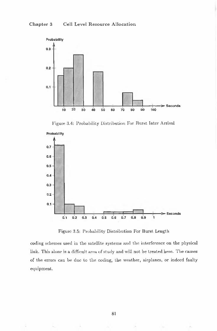
C h a p ter 3 C ell L eve l R eso u rc e A l lo c a t io n
Probability
j k0.3
0.2
0.1
!--- , 10 20 30 40 50 60 70 80 90 100
-5*- Seconds
Figure 3.4: Probability Distribution For Burst Inter Arrival Probability
0.7
0.6
0.5 -j
0.4
0.3 -|
0.2
0.1
0.1 0.2 0.3 0.4 0.5 0.6 0.7 0.8 0.9 1Seconds
Figure 3.5: Probability D istribution For Burst Length
coding schemes used in the satellite systems and the interference on the physical link. This alone is a difficult area of study and will not be trea ted here. The causes of the errors can be due to the coding, the weather, airplanes, or indeed faulty equipment.
81
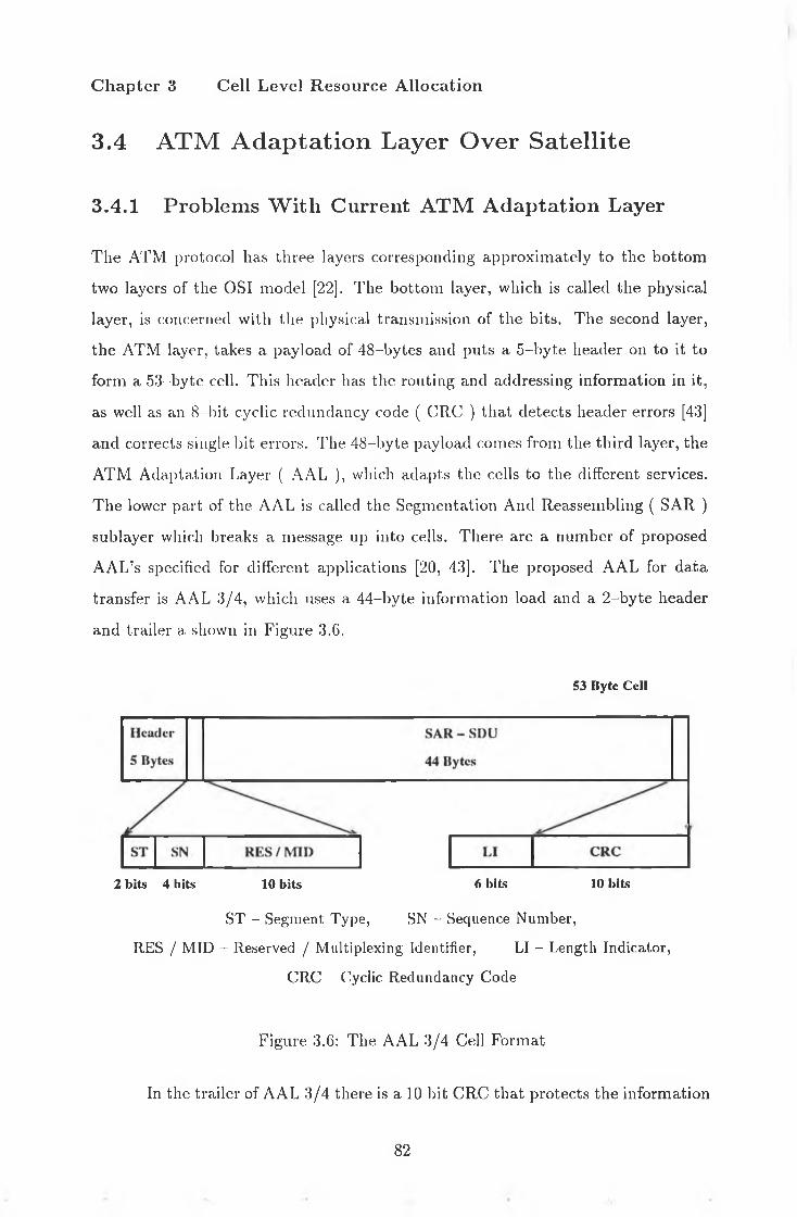
C h a p ter 3 C ell L eve l R e so u rc e A llo c a t io n
3.4 A T M A d a p ta tio n Layer O ver S a te llite
3.4 .1 P rob lem s W ith C urrent A T M A d a p ta tio n LayerThe ATM protocol has th ree layers corresponding approxim ately to the bo ttom two layers of the OSI model [22]. The bottom layer, which is called the physical layer, is concerned with the physical transmission of the bits. The second layer, the ATM layer, takes a payload of 48-bytes and puts a 5 -by te header on to it to form a 53-byte cell. This header has the routing and addressing information in it, as well as an 8 -b it cyclic redundancy code ( CRC ) th a t detects header errors [43] and corrects single bit errors. The 48-byte payload comes from the th ird layer, the ATM Adaptation Layer ( AAL ), which adapts the cells to the different services. T he lower part of the AAL is called the Segmentation And Reassembling ( SAR ) sublayer which breaks a message up into cells. There are a num ber of proposed A A L’s specified for different applications [20, 43]. T he proposed AAL for d a ta transfer is AAL 3/4 , which uses a 44-byte information load and a 2 -by te header and trailer a shown in Figure 3.6.
53 Byte Cell
2 bits 4 bits 10 bits 6 bits 10 bits
ST - Segment Type, SN - Sequence Number,RES / MID - Reserved / Multiplexing Identifier, LI - Length Indicator,
CRC - Cyclic. Redundancy Code
Figure 3.6: The AAL 3/4 Cell Form at
In the trailer of AAL 3 /4 there is a 10 bit CRC th a t protects the information
82

C h a p ter 3 Cell L evel R eso u rc e A llo c a t io n
load from errors. However due to the small CRC, the potential undetected error ra te is high. For the 10 bit CRC there are 210 different polynomials th a t can be used, no more. If the SAR SDU suffers an error there is then a 1 /2 10 probability th a t it will match the polynomial, or the undetected ra te could be as high as 10-3 . There is also no correction for double bit errors.
There is also another problem in th a t there are only four bits allowed for the sequence number. This means tha t there can be at m ost 24 S A R -S D U ’s ou ts tanding on the link, if there is to be a retransmission scheme working correctly. If the round trip propagation delay is 540 milliseconds then the m axim um throughput will be given by :
53 8 2*M aximum Bit ra te throughput = ---------- = 12,563 kbpsb 1 0.54 1This limits the m axim um transmission ra te for a single link. Even though there are methods tha t can be used to overcome this problem , it is a non-ideal solution, and the m axim um throughput should be larger. To get to a stage where you could have 155 Mbps throughput there would need to be 18 bits for the sequence number. This would impose 4.7% overhead, or an ex tra 3.6% overhead from the previous case, and this is probably unacceptably high.
3 .4 .2 P rop osed A T M A d a p ta tio n LayerIt is proposed here tha t it is more efficient to consider moving the CRC and the sequence num bers to the higher Convergence Sublayer ( CS ) [6]. By moving the sequence num ber to this layer larger blocks are got to pu t error detection and correction d a ta on. For the AAL 3/4 the overhead is about 8% b u t to modify tha t for a T1 satellite link an 11 bit sequence num ber would be needed. Also by moving the CRC to the CS level, and making it a 32 bit CRC, the unde tec ted error is reduced to less than IE-9. The ATM standards specify many A A L’s th a t can be used, bu t it is permissible to specify a different AAL for a particular application. It is suggestted here th a t high-speed, long-delay satellite links need a unique AAL. This can be achieved by inserting the sequence num ber and the CRC at the CS sublayer, requiring a type of framing. T he AAL th a t is proposed here is capable of
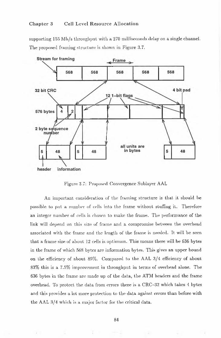
C h a p ter 3 C ell L eve l R e so u rc e A l lo c a t io n
supporting 155 M b/s throughput with a 270 milliseconds delay on a single channel. The proposed framing s tructu re is shown in Figure 3.7.
Figure 3.7: Proposed Convergence Sublayer AAL
An im portan t consideration of the fram ing s tructu re is tha t it should be possible to pu t a num ber of cells into the frame w ithout stuffing it. Therefore an integer num ber of cells is chosen to m ake the frame. The performance of the link will depend on this size of frame and a compromise between the overhead associated with the frame and the length of the fram e is needed. It will be seen th a t a frame size of about 12 cells is op tim um . This means there will be 636 bytes in the frame of which 568 bytes are information bytes. This gives an upper bound on the efficiency of about 89%. C om pared to the AAL 3 /4 efficiency of about 83% this is a 7.5% improvement in th roughput in term s of overhead alone. The 636 bytes in the frame are m ade up of the data , the ATM headers and the fram e overhead. To pro tec t the d a ta from errors there is a CRC-32 which takes 4 bytes and this provides a lot more protection to the d a ta against errors than before with the AAL 3 /4 which is a m ajor factor for the critical data.
84

C h a p ter 3 C ell L evel R eso u rc e A llo c a t io n
3 .4 .3 Service—B ased R etran sm ission Schem eIt is also proposed th a t there should be service selection to improve efficiency for reliable delivery. This is needed because rea l- t im e d a ta and voice usually cannot tolerate delays of one and a half times the round tr ip propagation delay. For example, voice will tolerate the 270 milliseconds propagation delay, bu t if it is in error, it will take another 540 milliseconds for retransmission, even assuming no congestion delay. The total delay is 810 milliseconds, which is unacceptable. Therefore there is no use in trying to detect errors or re transm it voice cells. In fact, any service tha t is delay sensitive in the sense of less than a few seconds is considered here to be real time and so is not fram ed for error detection and retransmission. For rea l- tim e services no framing is required. Even if the link is fully occupied the room for the retransmission of reliable d a ta is got by discarding some of the rea l- t im e cells, e.g., the voice cells. T he way in which the rea l- tim e cells mix with the fram ed cells is shown in Figure 3.8. It can be seen th a t the realtim e cells only enter the buffer if they expect to have less than a 50 millisecond queueing delay. Also the framed cells are kept in a t im e out buffer in case they are needed for retransmission.
Figure 3.8: Proposed Retransmission Scheme
It can be seen th a t the frame is at the CS sublayer and takes 568 bytes of user d a ta and adds 8 bytes of overhead to form a 12 by 48-by te frame to be split up by the SAR into 12 cells. The 8 bytes of overhead is m ade up of a 32-bit
85

C h a p ter 3 C ell L evel R e so u rc e A l lo c a t io n
CRC, which could be the s tandard IEEE 32-C R C [6]. There is a sequence num ber of 16 bits which allows a full 155 M b/s of d a ta on a link with the delay as given above and the size of frame chosen above. For the optim al size frame the error characteristics need to be known in advance, however the probability of b it error will be in the order of 10“ ' for satellite links, and possibly some degradation to around 10“ 6 should be allowed for. Knowing this and th a t the overhead on the frame is 8 bytes then the optimal frame size is 992 bytes which is in the same region as what has been chosen. It is shown in the results th a t a frame size of about 12 cells is a fair e s tim ate for the conditions of the channels investigated here. Also 12 cells in a frame corresponds reasonably well to the currently used NASCOM standard block size of 4800 bits [50]. The algorithm th a t the t ransm itte r uses to send framed and rea l- tim e cells in shown in Figure 3.9.
SourceL
rData
Get 568 Bytes Check Space in Buffer
I
1Real Time (Voice)
Check Buffer Space
rNot OK
Discard Voice Cells Check Space in Buffer
OK
Not OK Discard Data Frame
rOK
Queue in Buffer Number Frame
Put in Timeout Buffer Transmit
1Not OK
Discard Voice Cell
Figure 3.9: T ransm itter A lgorithm For Selective Retranmission
At the receiver there is a problem when a cell is lost in th a t it is not known whether it is a voice cell or is one of the fram ed cells. If the cells from one frame are sent back to back on the link then these problems would not occur, bu t tha t takes away from a lot of the advantages of ATM. Instead the VCI gets the cells in order for the framing. However when the header is lost there are problems. If the header could be decoded correctly then it would be possible to conclude from
86

C h a p ter 3 C ell L evel R eso u rc e A llo c a t io n
the VCI what type of cell it was. However with no header, all th a t is known is th a t a cell has been lost. W hat could happen if the cell were framed is th a t there would not be the required num ber of cells in the frame and the framing would loose synchronisation, To overcome this and to m aintain the framing synchronising, a one-b it flag is proposed, and this coupled with the VCI will show the s ta r t of the frame. This o ne-b it flag is the last bit of the cell, for fram ed cells, and tells whether the cell is the first in the frame or not depending on whether i t ’s a 1 or a 0. The algorithm th a t the receiver uses to receive framed and rea l- t im e cells in shown in Figure 3.10.
Reciever Make Cells
1Voice Data ErrorDone Make Frame Done
Check Start bit in Frame
OKCheck CRC |
X Not OKDiscard Cell
rCRC OK
Find Frame Number Send Acknowledgement
Done
CRC Not OK Discard Frame
Figure 3.10: Receiver Algorithm For Selective Retranmission
The efficiency tha t is gained from this proposed ATM adap ta tion layer is twofold :
1. there are only 8 bytes of overhead on a frame of 568 user information bytes and
2. there are the sequence num bers to transm it over long delay links which allows large th roughput and possible retransmission schemes to be implemented.
The gain in efficiency compared to AAL 3 /4 is th a t instead of carrying 528 bytes
87

C h a p ter 3 C ell L evel R e so u rc e A llo c a t io n
of user information bytes in 12 cells 568 bytes are carried, which is a 7.5% increase in efficiency over the whole frame.
3.5 S im ulation &; R esu lts For S a te llite A T M
3.5 .1 S im ulation D eta ilsThe proposed models were simulated using S E S /ivorkbench. SES / workbench is a discrete-event package tha t allows hardware and software simulation. The model of the retransmission scheme and the error probabilities here are created by use of the graphical interface. The SES /workbench, compiles the code to C and runs on a four-processor Sparc-Server 629. Each simulated d a ta point is the equivalent of 17 days on a T l satellite link, bu t ra ther than modelling the 2E+12 bits, only the burst events are simulated. This reduces the simulation to 5 E + 9 bits and further optimisation of the model compresses this to 5E +7 events. In real t im e this can take between 3 to 36 hours of run tim e as this configuration of com puting can execute between 400 to 5000 events per second depending on the complexity of the event and the detail of the model. In tota l 1300 hours of C PU tim e, or nearly 8 weeks continuously computing, was expended in the simulation tests. W ithou t the speed up in the modelling and simulation it would have taken at least 1000 years to get the equivalent results.
The model consists of the generation da ta cells, which are fram ed, and realtim e cells, as is shown in Figure 3.11. There is a buffer at the t ransm itte r , which varies in size, tha t can be used to influence the throughput. T he rea l- tim e source cells check the delay in the transm it buffer before joining the queue. If the delay is more than a specified value, in this case 50 milliseconds, then the channel is assumed to be in burst error and the cells are discarded.
The d a ta source generates cells, and these are framed together first. Then when a frame is ready this is a t tem p ted to be placed in the t ran sm it te r buffer, if there is space available. If the t ran sm itte r buffer is full, it checks to see if there are any rea l- tim e cells there, and if there are they are removed to m ake room for the
88

C h a p ter 3 C ell L evel R e so u r c e A llo c a t io n
u s s e i q : SE?/des ign ! . 1How
Module: diagramSubmodel: model
Transmitter Channel Receiver
Check_Delay
t t e r _ B u f t erData_Source
Data-InTime_Uut_But'f et
*[]___ if—Check_Delay Channel_Wi th_Noise
ime_Sink
D a t a _ S i n k
Make_Frame>,
ACK
Real_Time_Source
Figure 3.11: Simulation Model
fram ed d a ta cells. If there is still not enough room then the frame is lost. However if there is room in the t ransm itte r buffer, then the frame is added to the buffer and given a sequence num ber with modulo 65,563. When the frame is tran sm itted the frame is also kept in the t im e-ou t buffer in case it is needed for retransmission. This buffer is 111.3 kbytes, whirh accom m odates the two-way propagation delay plus a small processing delay.
The channel has two sources of noise, burst errors and Gaussian noise. At the receiver the rea l- tim e cells and all the errored cells are released, while the correct fram ed cells are kept to a t te m p t to make a frame. If any bits in the frame are in error, or if a cell is missing, which is seen by a missing one bit flag, then the whole frame is discarded. If the 32 bit CRC of the frame is okay then an acknowledgement is sent back to the transm itte r , through a channel in which it also m ay encounter errors.
W hen an acknowledgement arrives from the receiver, the frame which corresponds to th a t sequence num ber, is discarded from the t im e-ou t bufFer. Otherwise after the t im e-ou t delay, the fram e in the t im e-ou t buffer, skips to the head of the transm itte r buffer, after checking th a t there is sufficient room in the buffer,
89

C h a p te r 3 C ell L evel R eso u rce A llo c a t io n
and is re transm itted . If there is not sufficient space then rea l- t im e cells are discarded from the buffer, and if this does not release enough space then the fram e is discarded.
3 .5 .2 S im ulation R esu ltsIt is possible to guarantee delivery of the framed cells, with the given error probabilities by means of retransmission providing there is e ither excess bandw idth to allow for the retransmission or else the percentage of real t im e services is reasonably high. However if the mix of framed cells to re a l- t im e cells is high then some framed d a ta will be lost due to the burst errors. Tests were carried out for three types of errors, first only bursty errors, then only Gaussian errors, and finally for both Gaussian and bursty errors. For each of these types of errors the effect of the buffer size is investigated. Also, the effect of changing the framed d a ta mix on the cell loss is investigated.
For burst errors, the cell loss for framed d a ta varies depending on the mix of fram ed d a ta and 011 the t ransm itte r buffer as is shown in Figure 3.12. The cell-loss ra te for framed d a ta can be decreased to whatever value is required by either backing off the framed da ta mix or increasing the tran sm itte r buffer size. However as the percentage of framed d a ta gets toward 100% the effect of the buffer is small and the graph becomes almost vertical m eaning th a t e ither all the d a ta gets through or gets lost.
As the loss of framed d a ta cells is dependent on the mix of traffic types, it becomes im portan t to find the mix of framed da ta to unfram ed d a ta th a t allows all the fram ed d a ta to get through w ithout error. For b o th bursty error and Gaussian noise the buffer required for no framed d a ta loss is shown in F igure 3.13.
As expected, as the percentage of framed d a ta increases towards 100% the buffer size required for 110 loss increases fast and the buffer size becomes unreasonably large. It is therefore apparent th a t the best scheme is to have a reasonable mix of framed d a ta and rea l- t im e traffic.
Gaussian noise introduces mainly single frame errors for b it error ra tes lower
90
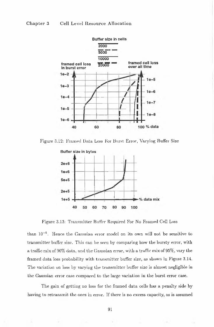
C h a p ter 3 C ell L eve l R e so u r c e A llo c a t io n
Buffer size in cells
2000
5000 "
10000framed cell loss 200™ in burst error
framed cell loss over all time
Figure 3.12: Framed D ata Loss For Burst Error, Varying Buffer Size Buffer size in bytes
Figure 3.13: T ransm itte r Buffer Required For No Framed Cell Loss
than 10- 5 . Hence the Gaussian error model on its own will not be sensitive to t ransm itte r buffer size. This can be seen by com paring how the bursty error, with a traffic mix of 90% data , and the Gaussian error, with a traffic mix of 95%, vary the framed d a ta loss probability with t ransm itte r buffer size, as shown in Figure 3.14. The variation on loss by varying the t ransm itte r buffer size is almost negligible in the Gaussian error case compared to the large variation in the burst error case.
The gain of getting no loss for the framed d a ta cells has a penalty side by having to re transm it the ones in error. If there is no excess capacity, as is assumed
91

C h a p te r 3 C ell L eve l R e so u r c e A llo c a t io n
Data loss in burst error
1 e-2
1e-4
1e-6
1e+5 2e+5 5e+5 1e+6 buffer sizein bytes
Figure 3.14: Effect Of Varying The Buffer Size
in this model, then there is going to be loss in the rea l- t im e cells. To see the effect of this loss, a plot of rea l- t im e cells, or voice cells, lost due to burst events for various transm itte r buffer sizes and against the fram ed d a ta mix is shown in F igure 3.15.
buffer size in cells
voice cell loss In burst error
5000 cells 10000 cells" 20000 cells voice cell loss
overall time2e-3
1e-3
5e -4
2e-4
1e-4
40 60 80 100 % data
Figure 3.15: Real T im e Cell Loss, Varying Buffer Size
In the burst event it is possible to lose all the voice cells if the mix of framed d a ta is high enough. This means th a t there is no more bandw idth available for retransmission. However this loss when averaged out over the day is of the order of
92
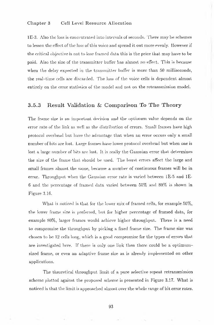
C h a p te r 3 C ell Level R e so u rc e A llo c a t io n
IE-3. Also the loss is concentrated into intervals of seconds. There m ay be schemes to lessen the effect of the loss of this voice and spread it out more evenly. However if the critical objective is not to lose framed d a ta this is the price th a t may have to be paid. Also the size of the transm itte r buffer has almost no effect. This is because when the delay expected in the tran sm itte r buffer is more than 50 milliseconds, the rea l- tim e cells are discarded. T he loss of the voice cells is dependent almost entirely on the error statistics of the model and not on the retransmission model.
3 .5 .3 R esu lt V alidation & C om parison To T h e T h eoryThe frame size is an im portan t decision and the op tim um value depends on the error ra te of the link as well as the distribution of errors. Small frames have high protocol overhead but have the advantage th a t when an error occurs only a small num ber of bits are lost. Large frames have lower protocol overhead but when one is lost a large num ber of bits are lost. It is really the Gaussian error th a t determines the size of the frame tha t should be used. T he burst errors affect the large and small frames almost the same, because a num ber of continuous frames will be in error. Throughput when the. Gaussian error ra te is varied between IE-5 and 1E- 6 and the percentage of framed d a ta varied between 50% and 80% is shown in F igure 3.16.
W hat is noticed is th a t for the lower mix of fram ed cells, for example 50%, the lower frame size is preferred, bu t for higher percentage of framed data , for exam ple 80%, larger frames would achieve higher throughput. There is a need to compromise the throughput by picking a fixed fram e size. The fram e size was chosen to be 12 cells long, which is a good compromise for the types of errors tha t are investigated here. If there is only one link then there could be a op tim um sized frame, or even an adaptive frame size as is already im plem ented on other applications.
The theoretical throughput limit of a pure selective repeat retransmission scheme plotted against the proposed scheme is presented in Figure 3.17. W hat is noticed is tha t the limit is approached almost over the whole range of bit error rates.
93

C h a p ter 3 C ell L eve l R e so u r c e A l lo c a t io n
no Gaussian noise
noise 1e-6 , 50% data mix
noise 1e-6 , 80% data mix
“ ise"l“ 5,“50% data mix
% Throughput noise 1e -5 , 80% data mix
Figure 3.16: Variation Of The N um ber Of Cells In A Frame
% Throughput
Figure 3.17: Comparison Of Proposed Scheme W ith Theoretical Limit
Therefore there is no need to use more complicated retransmission schemes [75] for these satellite links as there is only a small am ount of efficiency left to be captured with an increasing cost of transm itte rs and receiver protocols.
94

C h a p te r 3 C ell L eve l R eso u rce A llo c a t io n
3.6 C ell L evel C on gestion &: Traffic C ontrolT he primary role of traffic control and congestion control is to protect the network and the user in order to achieve network performance objectives. An additional role is to optimise the use of network resources. T he traffic control and congestion control mechanisms should not rely on other higher layer protocols which are either application or service specific to achieve the perform ance objectives required. However protocols may m ake use of the information in the ATM layer to increase their efficiency. The level of congestion control tha t is investigated here is concerned with the cell level. Given tha t there is congestion control used, what is of interest is the cell pa tterns th a t will cause the worst performance in the network.
3.6 .1 Traffic C ontract & U sage P a ra m eter C ontrolATM connections specify unidirectional Quality of Service ( QOS ) param eters. These param eters are specified at connection se t -u p and are guaran teed by the network. To guarantee the QOS, the network m ust be able to obtain enough information from the user about the connection and be able to ensure th a t no other connections th a t share the resources degrade the QOS. A user m ust enter into a contract with the network about the param eters of the connection. Then the network will im plem ent traffic control to avoid problems with degraded QOS before they occur. This includes Network Resource M anagem ent ( NRM ), Connection Admission Control ( CAC ) and Usage P aram eter Control ( UPC ). T he network will also control the case where congestion does occur by implementing Explicit Forward Congestion Indication ( EFCI ), selective cell discard and reaction to UPC failure.
W ithin the ATM cell there are a num ber of bits available for congestion and priority setting. These include the Payload Type ( P T ) indicator and the Cell Loss Priority bit ( CLP ) bo th of which are contained in the header of the ATM cell and can be seen in Figure 3.18.
The first bit of the P T indicator tells tha t the cell is a user cell and the next
95

C h a p ter 3 C ell L eve l R eso u rc e A l lo c a t io n
12
Bytes3
4
5
PT - Payload Type, CLP - Cell Loss Priority, HEC - Header Error Control
Figure 3.18: A Generic. ATM Cell Header
bit of it tells if congestion has been experienced by the cell in the network. The last bit differentiates between two different types of A T M -S D U ’s. The CLP bit is for high and low priority setting of the cells and can be done by the user and / or by the network. A cell entering the network with low priority is subject to being discarded by the network in times of congestion.
Traffic control is necessary to protect the network so th a t it can achieve the required performance objectives. UPC enforces a contract between the user and the network about the na tu re of the connection. This prevents any one user from causing excessive congestion th a t would degrade the quality of service provided to the other users. It is necessary to determ ine what is the worst traffic a user can inflict on the network while still abiding by U PC. T he Leaky Bucket A lgorithm is commonly used to implement the UPC function.
3 .6 .2 B asic A T M M od elA simplified ATM switch model consists of N users feeding a finite F irs t In First O ut ( FIFO ) buffer with B places and this is shown in Figure 3.19.
The arrival process from the users is random , bu t the U PC algorithm for worst case analysis makes the arrival process to the F IFO buffer deterministic. There are two types of arrival p a tte rns th a t are considered after the U PC and both
Bits8 7 6 5 4 3 2 1
Routing and Addressing
PT CLPHEC
96

C h a p ter 3 Cell L eve l R e so u rc e A llo c a t io n
Figure 3.19: Simplified Model
of them are periodic. The service process is also determ inistic ( at ra te r ). The worst case traffic, is tha t which creates the highest cell loss for a certain type of UPC, like the leaky bucket. A cell is lost when a cell arrives and gets through the U PC functions and finds tha t the buffer is full.
3 .6 .3 C onform ance D efin itio n — Leaky B ucketT he traffic contract specifies the negotiated characteristics of the connection. A connection traffic descriptor consists of 3 parts :
— the set of traffic, param eters in the source traffic descriptor— the cell delay variation tolerance
— the conformance definition
The conformance definition is used to decide which cells are conforming in an ATMconnection at the UNI [4]. A typical conformance definition is the leaky bucket [1]or Generic Cell Rate Algorithm ( G CRA ). The conformance definition should not be interpreted as the U PC algorithm, as the network provider may use any UPC as long as the operation of the UPC does not violate the QOS objectives of compliant connections. It is possible to use m any such algorithms together in tandem , and a typical im plem entation is the dual leaky bucket where there are two GCRA algorithms in series. The CAC will use the connection traffic descriptor to allocate resources and to derive param eters for the UPC. Any connection traffic descriptor m ust be enforceable by the UPC. Even though a cell is found to be non-conform ing
97

C h a p te r 3 C ell L evel R eso u rce A l lo c a t io n
th a t does not mean tha t the connection is not compliant. The precise definition of a compliant connection is left to the network provider. However a connection where all the cells are conforming m ust be specified by the network provider to be compliant. The traffic contract consists of the connection traffic descriptor and a requested QOS for each direction of the connection. T he private UNI m ay support a different traffic contract to the public UNI.
T he contract will contain the Peak ( ’ell R a te ( PC R ) and the cell delay variation as part of the source traffic descriptor, and will also contain the cell delay variation tolerance. Sustainable cell rate and burst tolerance are optional param eters. For best effort traffic the only p aram ete r specified is the P C R and the network may not reject the connection because th a t bandw idth is not available but it may impose a different PCR. CAC is used to decide if a connection should be accepted or continue to be accepted in the network. It is required th a t the traffic contract be accessible to the CAC so as to efficiently allocate resources. This access can be achieved by signalling for switched VCs or via a network m anagem ent system for perm anen t VCs. The prime concern is to achieve the required QOS for the new or re-negotia ted connection as well as to ensure tha t the connection will not degrade the QOS of all the other connections in the network. As well as deciding to accept the connection the CAC must determine the param eters needed by the U PC and route and allocate the. resources to the. connection. Even if high and low priority are not set the network may set them for non-conform ing cells.
The leaky bucket algorithm or GCRA has been standardised by the ATM Forum [4] for the conformance definition and it is formally defined as shown in Figure 3.20. There are a num ber of variables needed to define the algorithm. The Last Compliance Time. ( LCT ) is defined to be the last tim e th a t a conforming cell passed through the algorithm. How full the bucket is, is given by X the leaky bucket counter, and there is an auxiliary variable X* for predicting the value of the leaky bucket counter. The leaky bucket counter can pass cells conforming up to a limit given by L, and for each cell th a t is passed conforming the bucket is incremented by I. T he examination of the leaky bucket occurs when cell k arrives a t t im e t a(k). The variables L and I specify the operation of the algorithm.
98

C h a p ter 3 C ell L evel R eso u rce A l lo c a t io n
arrival of ccll k at time ta(k)
Non conforming ccll
Figure 3.20: Conformance Definition ( Leaky Bucket ) Algorithm
W hen a cell k arrives at t im e t.a(k) the variable X * is set to the value tha t the counter will have at this time. This is given by the previous counter value less the amount th a t the bucket will have leaked away since the last compliant cell, or X * = X — (■t a( k ) — LCT). If this is less than zero then the cell is compliant and the counter X * is set to zero and passes the cell. W hen a conforming cell is passed the counter X has to be updated by the increment I by X = X* + / and the last compliance tim e is the t im e of this cell, or LCT = t a(k). If the bucket has not completely leaked away then the bucket has to be checked to see if the limit is going to be exceeded or X* > L. If the lim it is not exceeded then the cell is conforming and the cell can be passed as before. Otherwise the cell is non compliant and no updates are done 011 the variables.
3.6 .4 Leaky B ucket A s T h e U P CU PC is the set of actions the network take to m onitor and control traffic. Even though the UPC definition is left to the network provider, it is likely th a t many network providers will use the leaky bucket to im plem ent it. This is because the same functions have to be carried out by the conformance definition and the UPC.
99
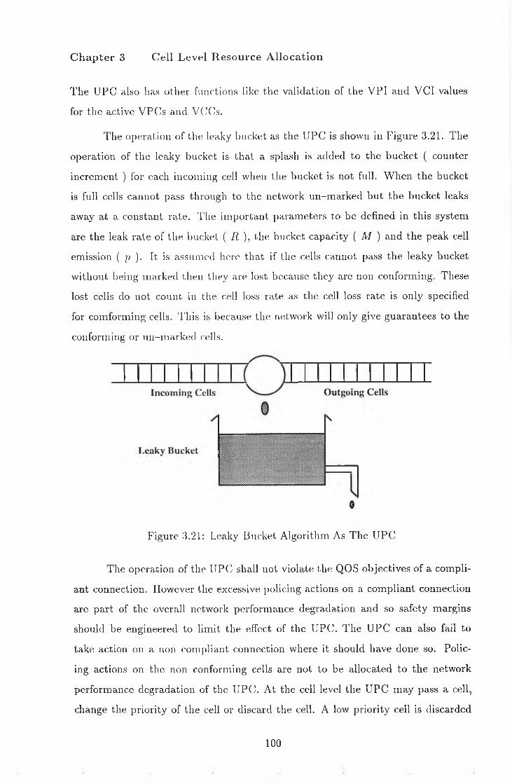
C h a p ter 3 C ell L evel R e so u rc e A llo c a t io n
The UPC also has o ther functions like the validation of the V PI and VCI values for the active VPCs and VC'Cs.
The operation of the leaky bucket as the UPC is shown in Figure 3.21. The operation of the leaky bucket is tha t a splash is added to the bucket ( counter increment ) for each incoming cell when the bucket is not full. W hen the bucket is full cells cannot pass through to the network un-m arked b u t the bucket leaks away at a constant rate. The im portan t param eters to be defined in this system are the leak ra te of the bucket ( R ), the bucket capacity ( M ) and the peak cell emission ( p ). It is assumed here tha t if the cells cannot pass the leaky bucket without being marked then they are lost because they are non conforming. These lost cells do not count in the cell loss ra te as the cell loss ra te is only specified for comforming cells. This is because the network will only give guarantees to the conforming or u n -m arked cells.
e
Figure 3.21: Leaky Bucket Algorithm As The UPC
The operation of the UPC shall not violate the QOS objectives of a compliant connection. However the excessive policing actions on a com pliant connection are part of the overall network performance degradation and so safety margins should be engineered to limit the effect of the UPC. The U PC can also fail to take action on a non compliant connection where it should have done so. Policing actions on the non conforming cells are not to be allocated to the network performance degradation of the U PC. At the cell level the U PC m ay pass a cell, change the priority of the cell or discard the cell. A low priority cell is discarded
100
C h a p ter 3 C ell Level R e so u rc e A l lo c a t io n
by the UPC if it is non conforming. Following the U PC, traffic shaping m ay be implemented on the conforming cells to reduce cell clumping. It is optional for the network operator to allow the UPC to initiate the release of a non compliant connection. Care must be taken when two levels of priority are used as the UPC may discard high priority cells. This can be the case even when if the U PC were placed only on the high priority cells they would be conforming. This is because the total of the two priorities are non conforming and there is the possibility tha t a previous low priority cell has been passed and so can not be taken back again.
The UPC and CAC are operator specific and should take into account the traffic contract to operate efficiently. It is specified tha t the signalling should take into account experimental traffic param eters tha t could be proprie tary to either the m anufacturer or network operator. It is optional to allow the operation of these param eters across the UNI by m utua l agreement. This could be achieved as before by either signalling for switched VCs or via a network m anagem ent system for perm anent VCs. It is optional for the user to be allowed to m ark cells as low and high priority. It is also optional for the network to m ark cells as low priority if they are not adhering to the traffic, contract. T he cell loss ratio for low priority cells must be higher than for high priority.
A commonly used UPC is a double leaky-bucket th a t controls the two different cell rates R and p, each with a separate, bucket. The peak ra te , p, is controlled by a bucket of size 1 and leak rate, p, and the second bucket operates as explained above. For a cell to be a conforming cell, it needs to be conforming with both buckets at the tim e i t ’s transm itted .
3.7 Issues For W orst C ase TrafficIt is of interest here to find the types of sources th a t can pass the conformance algorithm and produce the highest cell loss in the network when m ultiplexed together. This type of source will be called the worst case traffic. There are a num ber of issues arising when looking a t the worst case traffic.
101

C h a p ter 3 C ell L evel R e so u r c e A llo c a t io n
• The first item to consider is the potential types of sources tha t might produce high cell loss.
• The model of the buffer is im portan t as will be seen and there are a num ber of questions raised due to the use of infinite buffers. It is possible to use infinite buffers to approxim ately analyse random finite buffer systems, however this is not the case when the system is deterministic .
• There are fu rther complications due to the discrete na tu re of the problem. It is possible to simplify the problem by using continuous variable analysis and continuous variables but this can produce misleading results as can be seen by examining [23].
3.7 .1 T w o P o ten tia l W orst Traffic T y p esWhen considering which type of sources will produce the worst performance in the network while still m aintaining the con tract the first point to note is th a t the type of source will not allow the. leaky bucket to ever overflow. In other words the total available num ber of cells tha t are allowed to enter the network will enter to produce the lowest performance. Two types of sources th a t have been proposed tha t could be the worst types are a two s ta te source and a three s ta te source as shown in Figure 3.22.
The two s ta te source ( greedy on-off ) emits a burst of cells at the peak cell emission until the bucket is about to overflow and then falls silent waiting for the bucket to empty. This occurs periodically depending on the param eters of the system. T he three s ta te source is similar to the greedy on-off source except tha t it keeps em itting cells at the leak ra te after a burst. Therefore its operation is to emit a burst of cells a t the peak cell emission ra te until the bucket is about to overflow and then em it cells at the leak ra te of the leaky bucket for some tim e and then fall silent to allow the bucket to empty. This would then be repeated again. W hat can be seen is th a t the three s ta te source would have a longer period than the greedy on-off for the same system param eters.
T he general belief is tha t the greedy on-off source gives rise to the worst
102

C h a p te r 3 C ell L evel R eso u rce A llo c a t io n
Greedy O n-O ff
Ton Toff time
Three State
llllllll I I 1 II llllllll l l l l l ■Ton T* Toff time
Ton T* Toff time
Figure 3.22: Source Types
case traffic [83] as it would have the largest variance possible. However the three s ta te source has been proposed because it produces longer queues in an infinite buffer and therefore potentially larger loss in a finite buffer [84],
3 .7 .2 F in ite & Infin ite BuffersA study of the three s ta te source [84] compared i t ’s performance to th a t of the greedy on-off source, for a num ber of sources into an infinite buffer. W hat was found in those simulations is tha t the three s ta te sources produced higher buffer occupancy than the greedy on-off sources. The survivor function, P[Q > q], was found where Q was the buffer occupancy. This function was then assumed to approxim ate to cell loss in a finite buffer. However this would only be true for input traffic th a t would be statistically independent of the queue lengths, which is not the case here as the input traffic is periodic and determ inistic . It is possible to dem onstra te this fairly simply with a small example as is shown in Figure 3.23. Here the buffer occupancy for the infinite case of bo th the greedy on-off and the three s ta te is p lo tted on the same axis. Note th a t only a single source is being considered here on its own.
103

C h a p ter 3 Cell Level R eso u rc e A llo c a t io n
cell arrivals | | | | | | | | | | | | | | | | | |
cell arrivals | | | m | | | | | | I II II I
Figure 3.23: Buffer Occupancy In An Infinite Buffer
The period T of the greedy on-off is chosen to be half of the period of the three s ta te source so tha t it is possible to examine a single period of the three s ta te and compare it to two periods of the greedy on-off for cell loss. There are 2 cells arriving per cell tim e while the source is em itt ing at the peak ra te p and this continues until the bucket is full to capacity M , which in this example is 4. Then the bucket leaks away at a ra te of 1 cell per cell t im e R for the greedy on-off bu t for the three s ta te source it emits a t this ra te R for 6 t im e units, which is denoted by T* and here is equal to the period of the greedy on-ofF source. Look over 12 tim e units as both repeat exactly the same after this. Over this period there are12 cells inputted to the buffer which is the same as the leak ra te R multiplied by
104

C h a p te r 3 C ell L eve l R e so u r c e A llo c a t io n
the tim e period. The three s ta te source gives rise to higher buffer occupancy than the two sta te source as can be seen in Figure 3.23.
This would lead us to believe th a t the three s ta te source has higher loss compared to the greedy on-off source because of higher queue occupancy for the th ree s ta te source. W hen considering a finite buffer of capacity 2, as shown in Figure 3.24, it is found th a t the three s ta te source loses 2 cells, one at tim e period 1 and one at t im e period 2. However the greedy on-off source loses one a t tim e period 1 and one at t im e period 2 and again one at t im e period 7 and one at tim e period 8. So the cell loss ra te for the. three s ta te source is 0.166 while the cell loss rate for the greedy on-off is 0.333.
greedy o n -o ff
cell arrivals | m | | | | M | | | | | | | |
cell arrivals | | | | | | | | | | | | I I I I I I
12 three state
Figure 3.24: Buffer Occupancy In An Finite Buffer
105

C h a p te r 3 C ell L eve l R e so u rc e A llo c a t io n
The fact of higher buffer occupancy in the infinite case does not necessarily m ean higher cell loss rates in the finite buffer when the arrival process is dete rm inistic. For deterministic arrivals the loss in a finite queue is not necessarily related to the buffer occupancy in the infinite case bu t more on the m ethod of arrivals, or the process of arrivals, past the finite places in the queue. This problem was sim ulated [83] although the results were not explained.
3 .7 .3 C ontinuous & D iscrete V ariablesT he problem contains both continuous and discrete variables and therefore it is im portan t to distinguish between the two types. A simplified model is considered here which is similar to tha t published elsewhere in the lite ra ture [23] where there are two identical, independent users feeding a finite buffer. If the users were not independent then the worst case would be the greedy on-off source with all sources in phase em itting together. However when the users or sources are considered to be independent then the phase between the sources is random as shown in F igure 3.25. This then gives rise to the probability of cell loss because there is a probability of phase difference between the sources. The assum ption is m ade th a t the two sources are randomly phased, which m eans it is possible to consider one source as a reference source and the other one is then out of phase by some am ount. The am ount out of phase will determ ine the num ber of cells lost. The more in phase the more loss is expected. The probability of each of the possible combinations of out of phase is ju s t the reciprocal of the num ber of the possible combinations.
Two possibilities are considered here, e ither 2 greedy on-off sources or 2 th ree s ta te sources. The cell losses are calculated for every distinct com bination of the two traffic pa tterns in Sub-Section 3.8. To get the average cell loss for either case the losses are averaged. The cell loss ra te for each scenario is also com pared in Sub-Section 3.8. There are a num ber of constraints on the problem due to the discrete natu re of the variables which are described here :
1. T he sources may be out of phase only in cell t im e units which means th a t it
106
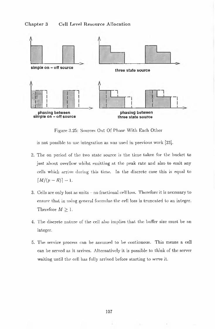
C h a p ter 3 C ell L evel R e so u rc e A l lo c a t io n
simple on - off sourcethree state source
mm■ i ' ih | i imm i i 1 >•
phasing between simple on - off source
I|
phasing between three state source
Figure 3.25: Sources O ut Of Phase W ith Each O ther
is not possible to use integration as was used in previous work [23].
2. The on period of the two sta te source is the t im e taken for the bucket to jus t about overflow whilst em itting at the peak ra te and also to emit any cells which arrive during this time. In the discrete case this is equal to\ M / ( p - R ) 1- 1 .
3. Cells are only lost as units - no fractional cell loss. Therefore it is necessary to ensure th a t in using general formulae the cell loss is trunca ted to an integer. Therefore M > 1.
4. The discrete natu re of the cell also implies th a t the buffer size must be an integer.
5. T he service process can be assumed to be continuous. This means a cell can be served as it arrives. Alternatively it is possible to think of the server waiting until the cell has fully arrived before s ta rt ing to serve it.
107
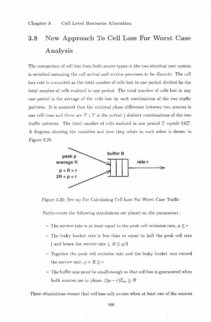
C h a p te r 3 C ell L eve l R e so u rc e A llo c a t io n
3.8 N ew A pp roach To C ell Loss For W orst C ase A n alysis
T he comparison of cell loss from both source types in the two identical user system is revisited assuming the cell arrival and service processes to be discrete. The cell loss rate is com puted as the total num ber of cells lost in one period divided by the total num ber of cells em itted in one period. The total num ber of cells lost in any one period is the average of the cells lost by each combination of the two traffic patterns . It is assumed tha t the minimal phase difference between two sources is one cell tim e and there are T ( T is the period ) d istinct combinations of the two traffic patterns. The total num ber of cells em itted in one period T equals 2R T . A diagram showing the variables and how they relate to each o ther is shown in Figure 3.26.
Figure 3.26: S e t-up For Calculating Cell Loss For Worst Case Traffic
Furtherm ore the following stipulations are placed on the param eters :
— The service ra te is at least equal to the peak cell emission rate, p < r— The leaky bucket ra te is less than or equal to half the peak cell ra te
( and hence the service ra te ), R < p / 2— Together the. peak cell emission rate and the leaky bucket ra te exceed
the service rate, p + R > r— The buffer size m ust be small enough so th a t cell loss is guaranteed when
both sources are in phase, (2p — r)Ton > B
These stipulations ensure tha t cell loss only occurs when at least one of the sources
108

C h a p ter 3 Cell L eve l R e so u r c e A llo c a t io n
is em itting at the peak rate. If the service process is assumed to begin as the cell is arriving this is called a fast server. Then the cell loss for two greedy on-off sources, x places out of phase with each other, is denoted by C L (x) and is calculated in Equation 3.1
C L ( x ) = \ { 2 p - r ) ( T on - x ) - B ] (3.1)
where the symbols have the usual meanings. W hen the two sources are on at their m axim um rate they exceed the service ra te by (2p — r) and so the queue is building up. This lasts for the am ount of tim e they are on at this ra te (Ton — x) and so the queue builds to (2p — r ) (T on — x) and so the loss is what this is in excess to the buffer size B. Hence Equation 3.1 is explained. Similarly the cell loss for the three s ta te source can be represented by Equation 3.2.
C L (x) = L(2 p - r ) (T on - x) + ( p + R - r ) (x ) - B \ (3.2)
The reason for the difference in the upper and lower bounds is due to the way in which the cells arrive at the end of the three s ta te source. T he upper bound, for the on-off source, is due to the fact tha t a fractional cell loss m eans th a t we have in fact lost tha t cell. A fractional cell loss in the three s ta te source comes from the overlap of the end of the peak ra te and the s ta r t of the m ean rate, b u t here they will not generate loss as the cells arrive as quick as the server can serve them . Therefore the lower bound is chosen.
Alternatively if it is assumed tha t the server waits until the cell has arrived in the buffer before starting to serve the cell, which is called the slow server, then the expressions for cell loss are modified for the greedy on-off source as follows in Equation 3.3
C L (x) = [(2p)(Ton - x ) - (Ton - * - 1 Jp)r - B ] (3.3)
W h a t is happening is tha t the t im e to serve has increased by l / p and so this m ust be included in the equations. For the three s ta te slow server the cell loss will be given in Equation 3.4.
C L ( x ) = [(2p)(Ton - x) - (Ton - x - 1 / p ) r + (p + R - r ) (x ) - B J (3.4)
109

C h a p te r 3 C ell L eve l R eso u rc e A l lo c a t io n
To calculate the cell loss ratio allow x to vary over all phase possibilities and then divide by the num ber of combinations and also divide by the num ber of cells t ransm itted by both sources. The num ber of cells tran sm itted by both sources will be 2R T and the num ber of phase combinations will be T, so the cell loss ratio, C L R , is given by Equation 3.5.
T - 1£ C L {x )CM = 1 w (3-5)
It is difficult to plot these equations due to the num ber of variable used and also because there are constraints on the variables th a t depend on the other variables. The constraints could be like Ton > x for cell loss to occur. Instead of a t tem pting to plot or sim ulate these equations, some examples will be provided.
3.9 C ounter E xam p les To T rad itional W orst C ase Traffic
To show th a t there is no single worst type traffic for two identical sources a counter example to the traditional theory of the greedy on-off being the worst case is presented. It is shown here tha t the three s ta te source can produce higher loss for integer values of variables chosen. As mentioned previously two different types of servers, the fast serving server and the slow serving server are considered.
3 .9 .1 Fast S erving ServerAssuming th a t the cell is served as it arrives here is an example showing the three s ta te source to give rise to greater cell loss in a finite buffer than the two sta te source. The following system param eters are used :
- p, peak cell emission ra te = 1
- r, service ra te = 1
- R , leaky bucket ra te = .5
110

C h a p te r 3 C ell L eve l R esou rce A llo c a t io n
- M , leaky bucket capacity = 8
- B , buffer size = 1 2
- T* ( for three s ta te source ) > ((2p — r )T on — B ) / ( p — R) = 6( Thi s is chosen so tha t there will be no loss when the two sources are out of phase by more than T* but there is a probability of cell loss if they are out of phase by less tha t T *. )
It takes 8 cell t imes to fill the bucket up but in th a t t im e 4 more cells are allowed through because of the constant leak rate of the bucket and while they try to fill the bucket 2 more arrive and then finally one arrives and the bucket is full. Therefore the am ount of t im e th a t the source is on and em itt ing cells at the peak rate is given by Ton = \ M / ( p — 7?)] — 1 = 15. When the bucket is full it takes M / R seconds to em pty normally, however here one tim e period has already elapsed so T0f j — 15.
There are 30 phase combinations for the greedy on-off source patterns , however sources th a t are too far out of phase do not give rise to cell loss. For the greedy on-off sources by examining Equation 3.1 sources th a t are 3 or more tim e units out of phase do not produce any cell loss. Rem em ber th a t this loss can occur when the second source is a little advanced from the reference and also when i t ’s so advanced th a t it is almost back in phase with the reference. This can be seen in Figure 3.27. T he cell loss for the two s ta te sources is in total 9 cells, which is calculated from 3 cells lost when in phase, 2 cells lost when either one ou t of phase and also 29 out of phase, and 1 cell lost when either two out of phase or 28 out of phase. For all o ther phases there is no cell loss. Get 9 cells lost in to ta l out of a possible 900 cells over the 30 phase and 2 sources. Therefore using Equation 3.5 the cell loss ratio can be calculated to be C L R = 0.01.
For the three s ta te sources cell there are 36 possible phase combinations and by examining Equation 3.2 loss can occur up to 4 units out of phase. The tota l num ber of cells lost over all 36 possible phases can be seen in F igure 3.27 and is 15 cells. By using Equation 3.5 the loss can be calculated to be C L R = 0.01157. Therefore the three s ta te source produces higher loss than the greedy on-off source for the fast server.
I l l

C h a p ter 3 C ell L eve l R e so u r c e A l lo c a t io n
Reference Source
timeOther Source with X = 0# Cells Lost 3 3
H i 1----- 1----- 1-----1------HX = 1 time
i 1--- 1----1--- rX = 2
# Cells Lost = 2 1 i 1--- 1--- 1----1- time
# Cells Lost =14--- 1--- (--- I--- 1----¥-
time(A)
Reference Source| , , , _ 4 _ h — |— |------------- p -
, , , , , v 3O ther Source with X = 0
-4-----1---- 1---- 1---- 1---- 1-----1---- k
time # Cells Lost = 3
X * 1time
# Cells Lost = 2
Figure 3.27: Fast Server: A. Greedy O n-O ff Source, B. Three S ta te Source
3.9 .2 Slow Serving ServerIf the service process is assumed to begin serving a cell only after it has fully arrived into the buffer here is a similar counter example. T h e following system param eters are used :
- p, peak cell emission ra te = 1
- r , service ra te = 1
- R, leaky bucket ra te = .5
112

C h a p ter 3 C ell L eve l R e so u rc e A llo c a t io n
- M , leaky bucket capacity = 8
- B, buffer size =14
- T* ( for three s ta te source ) > ((2p — r )T on — B + r / p ) / ( p — R) = 4
Similar to the fast serving server Ton = T0/ f = 15. For the greedy on-ofF sources by examining Equation 3.3 sources th a t are 2 or more tim e units out of phase do not produce any cell loss. This can be seen in Figure 3.28. T he cell loss for the two sta te sources is over all possible phase combinations equal to 4 cells and by using Equation 3.5 the cell loss can be calculated to be C L R = 0.00444.
Reference Source
O ther Source with X = 0 time
.....% # Cells Lost = 2 H 1--- 1--- 1----1-
X = 1
X = 2
# Cells Lost = 1 1--- 1--- 1--- 1--- 1----htime
time
h H i # Cells Lost = 0 -+— I--- 1--- 1—
(A) Ume
Reference Source
X = 2 time# Cells Lost = 1
1— 1— ---- 1---- 1---- 1---- 1-----1---- 1------------ o -X = 3
X = 4
I---1—I--1-
# Cells L ost = 0 -I 1---1---1---1-
# Cells Lost = 0 -I 1-----1-----1----- 1-----1 -
tlnic
time
Ume(B)
Figure 3.28: Slow Server: A. Greedy O n-O ff Source, B. Three S ta te Source
For the three s ta te sources cell loss can occur up to 2 tim e units out of phase. This is concluded by examining Equation 3.4 for the cell loss for a three
113

C h a p ter 3 C ell Level R eso u rc e A l lo c a t io n
sta te source and this is also seen in Figure 3.28. Here in total 6 cells are lost over all 34 possible phase combinations and so again by using Equation 3.5 the cell loss ratio can be calculated to be C L R = 0.00519. Therefore the three s ta te source produces higher loss than the greedy on-off source for the slow serving server.
Therefore regardless of how the service is achieved in the buffer there is an example of the three state source producing more loss than the greedy on-off source. It is therefore shown tha t there is no single type of worst case traffic source for the two identical source problem, considering these types of sources.
3.10 D iscu ssio nA num ber of issues have been dealt with here th a t arise when considering resource allocation at the cell level of the ATM. The s truc tu re of the adap ta tion schemes for satellites have been examined and the worst case traffic for the s tandard leaky bucket traffic controller has also been investigated.
It has been shown here tha t it is possible to use. ATM over satellite links. It is proposed here to place the error control in the convergence sublayer of the ATM ra the r than the segmentation and reassemble sublayer. This improves bo th the efficiency of the protocol and the efficiency of the error detection. T he moving of the error control functions is compliant with the ATM standards. It is also proposed here to differentiate the recovery mechanism, or re-transm issions, on the service. This allows a guarantee to be given to d a ta services of no loss while not affecting the real t im e services. While the simulation was for a T1 link, this approach can be incorporated into a da ta stream th a t is par t of a larger link, such as a 45 M b/s link.
From the analysis here, it may be concluded th a t the greedy on-off source does not always give rise to the worst case traffic. The first point th a t is m ade is regarding the infinite versus finite buffer and it is shown th a t the occupancy in an infinite buffer will not relate to the loss in a finite buffer when the traffic is deterministic. T he second point th a t is m ade here is th a t some of the variables are discrete and therefore a ttention m ust be paid when selecting examples and formula.
114

I
This is then concluded by showing two counter examples against the greedy on-ofF source and were able to say th a t there is no single worst case traffic type for the two identical source problem. The problem is far from totally solved as the result for this two source case is not binding on an 11 source situation, indicating one area of future work. On the other hand, the network needs to know what the worst case is in order to give the QOS to the users. This brings up the question of under what conditions is one case worse than o thers or if there is a single case th a t is not known abou t th a t performs universally badly for a given traffic controller. The progression could take either an analytical or simulation track, however care would be needed for e ither approach.
C h a p ter 3 C e ll L evel R e so u r c e A l lo c a t io n
115

Chapter 4
Pricing In ATM N etw orks
4.1 In trod u ctionAdmission control and bandwidth allocation are im portan t issues in telecommunications networks, especially when there are random fluctuating dem ands for service and variations in the service rates. In the emerging b roadband com munications environment these services are likely to be offered via an ATM network. In order to m ake ATM fu ture safe, methods for controlling the network should not be based on the characteristics of present services.
There are m any problems with traditional approaches to the connection admission control area. Users may not know enough about the sta tistics of their connections to provide accurate traffic descriptors to the network. This is particularly true for certain da ta transfers with long holding times. For example, in browsing a rem ote image database, it m ay not be possible to give a reasonable estim ate of the m ean bit ra te except over a long period of time. Even if users know their traffic descriptors they m ay be unwilling to reveal them , or m ay try to misrepresent them . This implies the need for some form of traffic policing and enforcement at the network access points, in order to ensure th a t each source is complying with what it declared at connection se t-up . Assuming accurate traffic descriptors, a complicated analysis is required to determ ine w hether sufficient resources are available to support the requested connection’s QOS while not degrading the QOS of adm itted connections. Current com putational m ethods cannot
116

C h a p ter 4 P r ic in g In A T M N etw o rk s
do this analysis on the short tim e scale in which CAC decisions m ust be m ade [80]. Consequently either simplifying assumptions about connection and resource interactions are introduced, or connections are grouped into classes whose members are assumed to have similar characteristics. Making simplifying assum ptions can lead to an over-controlled network, or produce unreliable results. For example, recent studies have shown tha t LAN and V B R video traffic is self-similar [45], which is very different to the behaviour predicted by Poisson-based or fluid flow models.
There is a trade-off between simplicity, which implies a small num ber of traffic classes, and the large num ber of classes needed to cover a wide range of different traffics and services. There is likely to be a wide variation in user requirements even within the same traffic class, due to individual preferences and internetworking considerations. Even if accurate traffic and network models were available, technological advances may quickly render their assum ptions invalid. For example, the bandwidth required for video or image transfer applications may continue to decrease due to improvements in compression / decompression algorithms and technology [3]. In addition, it is impossible to predict the characteristics of all fu ture applications, or the application mix when users become familiar with new network capabilities. It may be unwise to base CAC and bandw id th allocation schemes on the requirements and properties of current services.
ATM networks are expected to accom m odate a wide range of users including some who can tolerate a certain am ount of cell loss and / or delay. There are also likely to be some users who can modify their traffic inputs in response to feedback signals from the network. A feedback scheme is proposed to increase network efficiency by taking advantage of this flexibility.
The proposed approach here is based on pricing bandw idth to reflect network utilisation, with users competing for resources according to their individual bandwidth valuations. The prices m ay be components of an actual tariff or they may be used as control signals, as in a private network. Simulation results show th a t there is an improvement possible in term s of cell loss probability with the scheme here versus a more traditional approach, like the leaky bucket. This is p ar tly due to the fact tha t a closed-loop feedback scheme is being implem ented while the traditional
117

C h a p te r 4 P r ic in g In A T M N e tw o r k s
m ethods are open-loop schemes. In general closed-loop schemes can provide better utilisation than open-loop schemes. Simulation results here will show th a t a small queue with pricing can be efficient to m ultiplex heterogeneous sources. T he reason th a t only a small queue is needed is th a t once the num ber of cells th a t can be in excess in a feedback interval can be buffered, then the feedback can control the flows reasonably well. There is also consideration given to the economic efficiency of the network which addresses whether the traffic th a t is being carried is the most im portan t or not. There are other simulation results th a t show tha t it is possible to increase both the network utilisation and the economic efficiency together [53, 63].
Two fundam ental points about the approach here and pricing need to be spelled out :
• price is one possible feedback signal which has some a ttrac tive properties ( compactness, quantifiable, etc. ). Economists have developed a large body of theory on pricing mechanisms, and there is a lot of experience with the use of prices in real-world m arkets. However it is possible tha t there are other feedback mechanisms tha t , for one reason or another, m ay be preferable in communication networks. These other feedback mechanisms m ay be pricing schemes, like bandwidth auctions [51], or they might be traditional feedback schemes like Explicit Forward Congestion Indication, ( EFCI ), which eventually gets fed back to the user.
• when most people, think of prices, they think in m onetary term s, e.g. dollars and cents. However, there is nothing “inherently” monetary in applying pricing principles to communication networks. Pricing can be thought of as merely a m athem atica l framework or tool to be used to find the optim um operating point. O ther non-pric ing feedback schemes can be seen as special cases of the pricing scheme. For example the m ain reason th a t feedback will give the desired response is if the users change their traffic flows, and algorithm s th a t change traffic flows according to signals from the network can be modelled as an economic system. As long as the appropriate cost and valuation functions can be defined, a pricing m echanism can be applied even if money is not directly involved. An example is a private network where
118

C h a p te r 4 P r ic in g In A T M N etw o rk s
one organisation controls all the users. Here the valuation functions could be based purely on seniority. In this case the users ( or their applications ) are co-operative and can be programmed to obtain a desirable traffic mix. Of course some incentives are needed to ensure th a t the users respond as if the prices were going to be applied to their usage, b u t these incentives could be based on aggregated usage or some other indirect measure.
This chapter is organised as follows. In Section 4.2 the users are examined in detail in this light and they are re-classified using a new param ete r called adaptive. There are a num ber of new types of users investigated which can use a feedback signal from the network to control themselves and these are used in the rest of this chapter. In Section 4.3 there is the motivation for pricing in networks and in particular how to use price as a feedback signal and how price might be par t of the overall charging scheme. In Section 4.4 the m athem atica l model is built for the pricing and the benefit functions. First the user benefit function is addressed, and then the system or network problem. Then a proposed d istributed pricing algorithm is discussed. The following section, Section 4.5 deals with the network efficiency simulation model, the simulation environm ent and the results of the simulation. How to actually implement the pricing scheme suggested in shown in Section 4.6. There the generation of the price, the passing of the price from the network to the user and how the user uses the price to control the source is discussed. The idea of having both network and economic efficiency is discussed in Section 4.7 which starts off with an economic framework and the user models th a t might exist. In particular two of the five possible types of users are modelled, the elastic and inelastic users. Then another algorithm for pricing is proposed and the simulation details and the results are presented. In Section 4.8 it is shown where pricing fits into the overall picture of control of resources at the connection level. Finally in Section 4.9 there is some discussion of the chapter.
119

C h a p ter 4 P r ic in g In A T M N etw o rk s
4.2 A d ap tiv e C on n ection s
4.2 .1 D efin in g S ervices In A n A T M N etw orkAn ATM -based network is expected to allow users to negotiate their own service definitions. In this way a user can get a service appropria te to their individual needs. This assumes tha t some users will take a m ore active role in defining their network services than in p resent-day networks : these users are assumed to enter into negotiations with the network at the connection level, whenever a new connection is requested.
Some applications require guarantees from the network, on loss or delay or both. The user-network relationship for these applications in m any of the proposed Connection Admission Control ( CAC ) schemes is a contract : users describe their traffic and make QOS dem ands, and the network provides a s ta ted level of service while enforcing the user com m itm ents. When a new connection is requested, the network must decide whether or not to accept the connection; and if so, how to route it through the network and what resources to reserve for it. The connection request is refused by the network if accepting it would lead to QOS degradation for one or more currently-active connections which are complying with their contracts. Some CAC schemes provide feedback on the. reason for the refusal [25], which guides the user in subm itting a revised request.
Early CAC schemes reserved the peak bandw idth needed by an accepted connection - deterministic multiplexing - as required for c o n s ta n t -b i t- ra te ( CBR ) sources. However the gain in network utilisation possible by taking advantage of the statistical natu re of v a r iab le -b i t- ra te ( V BR ) sources has led to the idea of statistical multiplexing. S tatistical multiplexing is where it is possible to assign less than the peak bandw idth required bu t cell loss a n d /o r delay m ay be introduced.
The aim of a preventive CAC scheme is to balance the QOS provided to adm itted connections against network utilisation by limiting the num ber of connections using the network. Most proposed CAC schemes decide whether or notto accept a connection request based on knowledge of the traffic description, the
120

C h a p te r 4 P r ic in g In A T M N etw o rk s
u se r’s QOS requirements, and the current state of the network :
• ideally a user requesting a connection would give a com plete statistical description of their traffic, b u t in practice only a lim ited indication of expected behaviour is feasible. Connection behaviour is described by a set of param eters called traffic descriptors, such as mean b i t - ra te , peak b i t - ra te , m axim um burst length, probability of cell arrival in a fixed interval, and so on.
• user QOS requirements are usually expressed by networks researchers in terms of acceptable cell loss, delay and j it ter . How to relate these quantities to param eters the user is concerned with ( such as p icture quality in a video call ) is an active area of study.
• the current s ta te of the network can be determ ined by m onitoring the utilisation of network resources an d /o r by characterising the behaviour of connections already adm itted .
Based on this knowledge, CAC schemes have been proposed in which an effective bandw idth [39] is associated with each source in order to m eet its QOS requirements while still perm itting a statistical multiplexing gain.
Accepted connections are provided with a traffic contract and as long as they comply with tha t contract, their cells are treated as high priority by the network. Cells subm itted in excess of their contract may be discarded at the network access point, or m ay be m arked as low priority and discarded if the network is congested. Therefore the network provides no guarantees for low-priority traffic.
Not all applications require guarantees from the network. For example, some types of non -rea l- t im e d a ta transfers can tolerate a certain am ount of cell loss; or the application may recover from cell loss or delay at a higher layer of the protocol stack. These b e s t —e ffo r t applications request an Unspecified QOS service [4], in which the network always accepts the connection request bu t m ay assign a different Peak Cell Rate ( P C R ) than what was requested ( for example, a connection may be assigned a P C R of zero ). Cells which are subm itted in excess of the P C R are m arked as low priority.
121

C h a p te r 4 P r ic in g In A T M N etw o rk s
4 .2 .2 A daptive U ser B ehaviourIn the previous Sub-Section, network services were divided into “guarantees required” and “best-effort” , and an enforceable traffic description was needed from users who wanted guarantees from the network. This breakdown of services does not capture all possible user desires now, let alone in the future, because it does not account for a d a p t i v e users. A user is adaptive if they are able and willing to respond to feedback signals from the network during their connection lifetime by changing their offered traffic. The addition of w illingness-to-respond reflects the fact tha t some users may run applications which are capable of adaption, b u t do not want to be concerned with network feedback during the connection. A typical adaptive scheme is where there is a limited set of traffic param eters given to the network and the network gives a lim ited set of QOS to the user. However these param eters may not affect the user bu t would affect the user’s term inal equipm ent and would be instructed in advance by the user on how to adapt to the network feedback signals. Not all users will be adaptive and therefore the network will conta in a m ix ture of user types. Two types of users, an adaptive and non-adaptive , are shown in Figure 4.1. A user who is willing to wait ( based on network feedback ) to set up their connection but who wishes to be insulated from such feedback once the ir transmission starts is adaptive only at the connection level, and such users are not regarded as adaptive.
User / Network
Figure 4.1: Proposed Adaptive Feedback Scheme
122
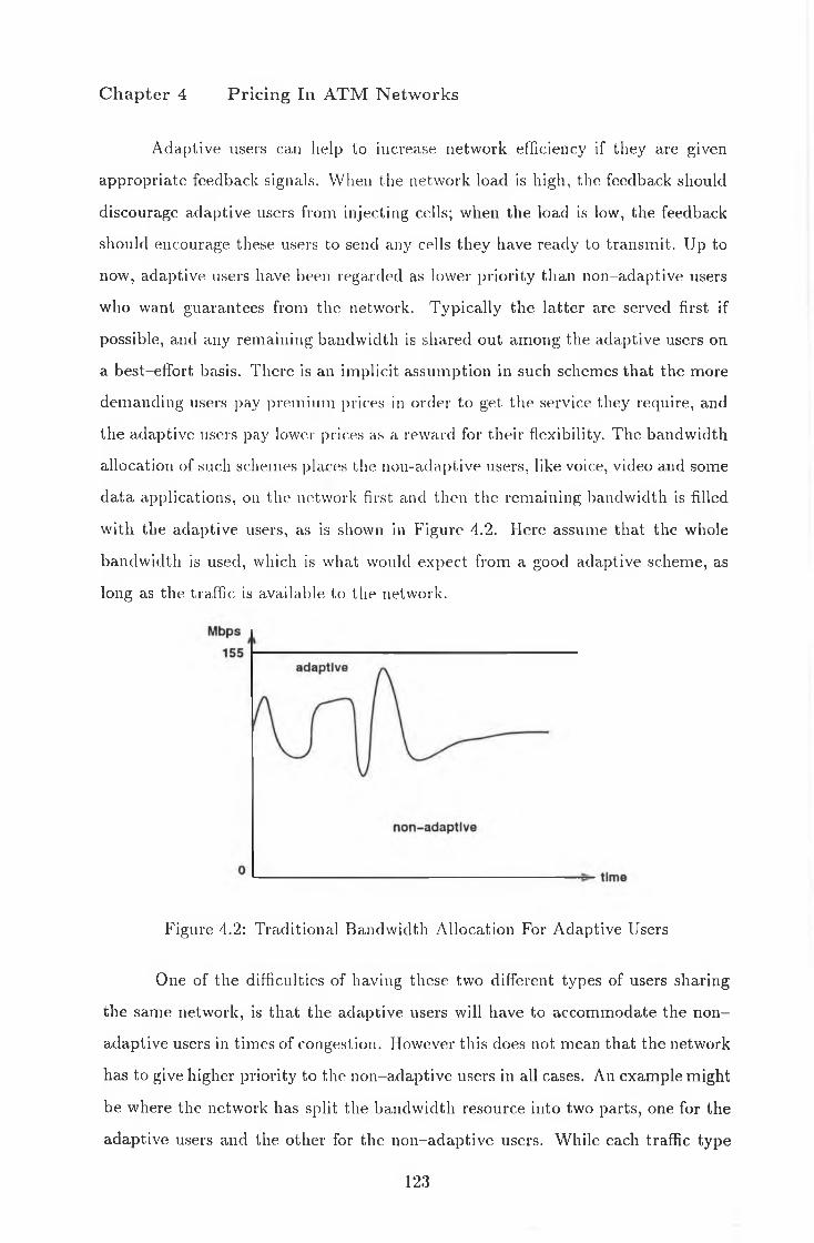
C h a p ter 4 P r ic in g In A T M N etw o rk s
Adaptive users can help to increase network efficiency if they are given appropriate feedback signals. W hen the network load is high, the feedback should discourage adaptive users from injecting cells; when the load is low, the feedback should encourage these users to send any cells they have ready to transm it. Up to now, adaptive users have been regarded as lower priority than non-adaptive users who want guarantees from the network. Typically the la t te r are served first if possible, and any remaining bandw idth is shared out among the adaptive users on a best-effort basis. There is an implicit assum ption in such schemes tha t the more dem anding users pay prem ium prices in order to get the service they require, and the adaptive users pay lower prices as a reward for their flexibility. The bandw idth allocation of such schemes places the non-adaptive. users, like voice, video and some d a ta applications, oil the network first and then the remaining bandwidth is filled with the adaptive users, as is shown in Figure 4.2. Here assume tha t the whole bandwidth is used, which is what would expect from a good adaptive scheme, as long as the traffic is available to the network.
Figure 4.2: Traditional Bandwidth Allocation For Adaptive Users
One of the difficulties of having these two different types of users sharing the same network, is th a t the adaptive users will have to accom m odate the n on - adaptive users in times of congestion. However this does not mean tha t the network has to give higher priority to the non-adap tive users in all cases. An example might be where the network has split the bandw idth resource into two parts , one for the adaptive users and the o ther for the non-adap tive users. While each traffic type
123

C h a p ter 4 P r ic in g In A T M N etw o rk s
is within i t ’s own part of the bandwidth, it has high priority, bu t when it uses the o th e r’s par t of the bandwidth then it has low priority. In Figure 4.3 it can be seen tha t the non-adap tive users have been allocated 100 Mbps of bandw idth and the adaptive users are allocated 55 Mbps. W hen the adaptive users fall into the 100 Mbps of the non-adap tive users bandwidth, then their priority is changed from high to low. However when the non-adaptive users use p a r t of the 55 Mbps of the adaptive users bandwidth then their priority is changed from high to low. However the adaptive scheme will lower the adaptive users input traffic to accom m odate the variations in this non-adap tive traffic.
Figure 4.3: Exam ple Of Priorities For Two Traffic Classes
W hether or not a network operator gives higher priority to more dem anding users is a policy or business decision, not a technical one, and it is not the intention here to argue for one side or the other. From a technical point of view it is as easy to give either higher priority. Naturally there are technical implications in giving one or the other higher priority. For example network dimensioning changes depending on the priority allocation. However, technical problems do arise when some adaptive users also require guarantees on cell loss. For example, d a ta transfers using compression m ay be very flexible with respect to delivery t im e bu t require zero cell loss to ensure d a ta integrity, if there is l it tle or no redundancy in the transm itted data. The classical approach to such users is to re transm it when errors occur, but in congested conditions this approach tends to increase the network load and worsen the congestion. This is especially true when the d a ta is p rotected by
124

C h a p ter 4 P r ic in g In A T M N etw o rk s
some higher layer protocol and one cell loss may m ean tens or hundreds of cells have to re transm itted as the block of d a ta tha t has to be re tran sm itted is much larger than the cell. This would mean th a t in times of congestion ra ther than run the risk of loss it would be b e t te r to delay the transmission of the data .
A novel idea is to provide a limited set of guarantees to adaptive users who require them. This could be giving loss guarantees to an adaptive user th a t can wait to send the cells. The network would give the guarantees by informing the user when there is a low load and therefore no expected cell loss in the network. However this is a difficult problem, since adaptive users cannot give an accurate traffic description at connection se t-up , the traffic they send depends in some way on network conditions at the tim e their application generates it. Before the proposed solution here is described to this problem, a discription of general classification of user types which includes adaptive users is done.
4 .2 .3 P ossib le T y p es O f U serFour criteria for classifying user types are considered here ( o ther criteria m ay also be useful and it is not claimed here th a t all possible user behaviour are described ) :
• a traffic description - in terms of network traffic descriptors - is available at connection set-up;
• guarantees are required on cell delay. Since the user knows ( or can determine ) their own processing delays, the applica tion’s delay tolerance can be translated into a m axim um acceptable delay within the network;
• guarantees are required on cell loss. In practice this means th a t the network guarantees to t rea t the user’s cells as high priority;
• the user is adaptive, in the above sense
This classification is sum m arised in Table 4.1.
Some of the entries in Table 4.1 can be ruled out as follows :
125

C h a p te r 4 P r ic in g In A T M N etw o rk s
Table 4.1: Classification Of User Types
Type AdaptiveTraffic
DescriptorLoss
G uaranteeDelay
G uarantee1
YesYes
2Yes
No3
NoYes
4Yes
No5
YesYes
6No
No7
NoYes
8 No9
YesYes
10Yes
No11
NoYes
12No
No13
YesYes
14No
No15
NoYes
16 No
• for non-adap tive users, a traffic description is required in order to get guarantees on loss an d /o r delay. Therefore rows 13, 14 and 15 can be eliminated;
• for non-adap tive users who provide suitable traffic descriptors to the network, combine the cases where they require guarantees. Therefore rows 9, 10 and 11 can be combined into a single user type;
• for users who do not require guarantees, no traffic descriptor is needed ( it is possible to think of these users as m arking all their cells to be low priority, as if they had been given Unspecified QOS service with a zero P C R ). Therefore rows 4 and 12 can be eliminated;
126

C h a p te r 4 P r ic in g In A T M N etw o rk s
• by definition, adaptive users do not have a traffic descriptor at the s ta r t of a connection. Therefore rows 1 — 4 can be eliminated;
• adaptive users who require guarantees on loss and delay have to decide a m inim um acceptable bandwidth. This is because it is not possible for the network to give guarantees to a user who cannot describe its characteristics and has to send the. cells immediately and requires a certain loss probability. So this type of user essentially converts their traffic into a non-adap tive component which has a traffic, descriptor and requires loss and delay guarantees ( row 9 ), and an adaptive component which requires no loss guarantees ( row 7 ). Therefore row 5 can be eliminated.
Table 4.2: Expected User Types
Type Old Type AdaptiveTraffic
DescriptorLoss
G uaranteeDelay
G uarantee1 9 ,1 0 ,1 1
NoYes
2 16 No3 8
Yes No NoNo
4 7 Yes5 6 Yes No
W hen these entries are eliminated, the user types shown in Table 4.2 are left. A particular user can divide their traffic input into one or more of these types :
1. n o n - a d a p t i v e , requ ires g u a r a n t e e s , h as a t ra f fi c d e s c r i p t i o n a t c o n n e c t i o n s e t - u p . This is one of the user types addressed by various proposed CAC schemes, so it will not be discussed fu rther in this work.
2. n o n - a d a p t i v e , no g u a r a n te e s requ ired . This is non-adap tive b e s t - effort traffic, such as the traffic a user injects in excess of their contract with current CAC schemes.
127

C h a p ter 4 P r ic in g In A T M N etw o rk s
3. a d a p t i v e , n o t d e l a y - s e n s i t i v e , n o lo s s g u a r a n t e e s requ ired . This type of user waits until feedback from the network indicates th a t the load is low, then sends cells on a best-effort basis. This could be implemented by negotiating a traffic contract specifying zero mean and zero peak rates. Then there is no reservation of resources and all cells will be marked as low priority. These users are called a d a p t i v e b e s t —e ffo r t users here.
4. a d a p t i v e , d e l a y - s e n s i t i v e , n o loss g u a r a n t e e s requ ired . Thistype of user responds to network feedback by modifying how m any cells they transm it, b u t sends them immediately on a best-effort basis. Otherwise they are similar to adaptive best-effort ( type 3 ) users, and they are called in e la s t i c users.
5. a d a p t i v e , n o t d e l a y - s e n s i t i v e , r e q u i r e s lo ss g u a r a n t e e s . Thistype of user waits until feedback indicates the network is lightly loaded, then transm its and requires tha t their cells are not lost in the network. These users are called e la s t i c users here.
The names th a t are given to the types th a t are listed in Table 4.2 are shown in Table 4.3 with a description.
Table 4.3: Description Of Expected User Types
Type Name Description1 Normal N on-A dap tive Guarantees2 Best-Effort N oil-A daptive No Guarantees3 Adaptive Best-Effort Adaptive No Guarantees4 Inelastic Adaptive Delay G uaranteed5 Elastic Adaptive Loss G uaran teed
Traditionally the view has been th a t w ithout an enforceable traffic description, no guarantees can be expected of the network. One possibility is tha t bursty sources can be well-described during a burst. T he need for burst- level CAC has
128

C h a p te r 4 P r ic in g In A T M N etw o rk s
been widely discussed, e.g. [70, 80]; however burst s ta r t t im e and duration can be unpredictable.
The view is taken here th a t adaptive users can be accom m odated with a f a s t r e s e r v a t i o n scheme. A form of in-connection negotiation is proposed here, on a tim e scale shorter than the dynamics of connection se t-up and tear down but longer than cell-sc.ale effects. Elastic users who comply with these dynamic contracts transm it h igh-priority cells in the interval between successive feedback signals from the network.
4 .2 .4 Feedback—B ased Fast R eservationIdeally, feedback would be provided continuously to adaptive users. In practice the signalling and com putation required means tha t time m ust be divided into feedback intervals. Feedback intervals on the order of a millisecond are expected here, so the adaptive user responses would have to be autom ated.
At the sta rt of each feedback interval, the network sends a signal to each adaptive user. T he responses of inelastic and adaptive best-effort users were outlined in the previous Section. Elastic users presum ably have an application- dependent deadline by which transmission m ust be completed or the application will be aborted; assume this deadline is long-term compared to the feedback dynamics and therefore is not a factor in their response to the feedback signals.
Based on the feedback signal and their application requirements, each elastic user signals the network with the num ber of cells they wish to transm it in this feedback interval. T he network uses buffers to take care of possible cell-scale congestion, and decides if it can accom m odate each elastic users request with zero cell loss. If not, the request is denied and the user waits until the next feedback interval to try again ( they can also transm it the cells immediately, a t low priority, bu t tha t essentially converts them into adaptive best-effort users ). If an elastic user’s request is accepted, then they transm it their cells with high priority during the feedback interval and are guaranteed th a t the network will not lose those cells. A mechanism is probably needed to enforce the user requests, since otherwise users
129

C h a p te r 4 P r ic in g In A T M N e tw o r k s
who are accepted but decide not to t ransm it unnecessarily block o ther users.The main problem with this kind of dynam ic contract negotiation is tha t
the network has to do the corresponding com putations every feedback interval. If the users contending for shared network resources are geographically separated, the tim e to do the required signalling may be excessive even if the necessary com putational power was available, and the feedback scheme would be potentially unstable.
One possibility is to localise the contention, for exam ple by deterministi- cally multiplexing the V P ’s within the network. This reduces the network to a set of “virtual channel connections” between source-destination pairs : the capacity of each such virtual channel connection is fixed for the feedback interval, and interactions within the network between traffic stream s corresponding to different source-destination pairs are eliminated. Therefore the only contention between users is at the network access points. W hile this model is a first cut, two points should be noted :
• the loss of efficiency by not statistically multiplexing the V P ’s within the network may be outweighed by the increased efficiency obta ined by using feedback to multiplex the users a t the network edges;
• the V P capacities could also be updated , on a longer t im e scale than the feedback intervals, to match overall dynamics of network traffic.
4.3 M otiva tio n For P r ic in gMost researchers divide users into classes according to their application requirem ents and traffic characteristics; for example, rea l- t im e video, re a l- t im e audio, stored (off-line) video, and off-line d a ta transfer. Each class is then regarded as having a generic, user for analytical purposes. Users are usually assum ed to be capable of negotiating a “contract” at connection se t-up , which specifies their traffic param eters and service level. T he network then polices the offered traffic and enforces the contract if users misbehave.
Two obvious user characteristics are usually ignored :
130

C h a p te r 4 P r ic in g In A T M N e tw o r k s
• even within a class, user preferences can be expected to be heterogeneous. If this “in ternal” variation within a class is substantial, then any assumptions about generic user behaviour will be inaccurate for m any users in this class. One way to capture this heterogeneity is to say th a t users value their network service differently, according to their subjective requirements for the quality of their application.
• some users may be capable of responding to control signals from the network during their connections, not ju s t at connection se t-up . Users are par t of the network and in many cases can be thought of as intelligent peripheral devices at the network edges. These intelligent peripherals can regulate how much and when traffic, is input, given appropriate indicators of the network status.
4 .3 .1 P ric in g B an d w id thT he system m ade up of the users together with the network has various resources th a t can be used to meet .service dem ands. However in all realistic systems these resources are lim ited and some m ethod of allocating them is needed when total dem and is greater than the resource limit. The resources are the capacities of the ATM connections. The bandw idth allocated to a user is considered to be a com modity which is sold by the network to the user [19, 52, 54]. The view here is tha t the users place a benefit, or w illingness-to-pay, on the bandw idth they are allocated. Given a price per unit of bandw idth , a user’s benefit function completely determines th a t user’s traffic, input. Users are assumed to act in their own best interests and to be capable of responding to changes in the price for bandwidth.
In the formulation here, network constraints such as virtual p a th capacities [13] are transla ted into cost functions on the bandw idth demands. This is because one user’s consumption of bandw idth gives rise to fairness issues involving all the other users. This can be represented as a social ‘cost’ ( in term s of longer delays, less available bandwidth, etc ) which is borne by all users. The network operator sets the prices so th a t the m arginal benefit the users place on their band-
131

C h a p ter 4 P r ic in g In A T M N etw o rk s
widths is equal to the marginal cost of handling tha t traffic in the netw ork1. The network operator dynamically adjusts the prices based on m onitored network conditions. T he assumption here is tha t when the price of bandw idth increases, users reduce their dem ands. There is no need for enforcement of connection param eters in the scheme here because users do not declare anything about their traffic.
A typical configuration tha t is envisaged is shown in Figure 4.4. T he user programs the term inal equipm ent with their benefit function. T he bandwidth in cells per second allocated to the user by the network depends on this benefit function and the price tha t is sent from the network to the term inal equipm ent.
User Terminal Network Access
Network Interface
Figure 4.4: Proposed Configuration For Access
T he approach here is intended to be applicable to general ATM networks and to the full range of user and service types, such as voice, video, rea l- t im e data and non-tim e-sensitive data. However a special case th a t is particularly suitable is th a t of a V irtual Private Network ( V PN ) in which one opera tor controls the network and all applications running on it. Why this is special is because when there is a single operator it is possible to implement pricing algorithms on all user nodes even without having any charging taking place. In a public network it would not be possible to ensure tha t all users would install the algorithms in the first place and then run them without tam pering with them . T he relative im portance of various applications in the V PN could then be varied over t im e and from node to node. For example, the operator may place a high priority on operational data transfer and low priority on other d a ta transfers; or interactive video and voice
10nly address the variable costs corresponding to network constraints. The recovery of fixed network costs could be done by an access charge or some other method.
132
C h a p ter 4 P r ic in g In A T M N etw o rk s
might get higher priority than other traffic types.Dynamic priority assignment is where the priority can change from one ap
plication to the next, or even during an application, for the sam e type of application. This can be used to differentiate between the im portance of even the same types of applications. However assigning dynamic priorities is difficult. W h a t is also needed is adaptive priority assignment so th a t it could be possible to give real t im e services priority if there is no chance of loss bu t change to give d a ta applications priority if there is likely to be loss. For example if the rea l- tim e applications such as voice and video are given priority to ensure timely delivery, then d a ta traffic may suffer higher loss though it may not be able to tolerate cell loss as well as voice. On the other hand, if priority is given to d a ta and large buffering is employed, then rea l- t im e applications may suffer large variable delays.
W hat is needed is a dynam ic adaptive in te r-tem poral priority scheme. The priorities should change to track changes in the network s ta te or in the application requirements over multiple tim e periods. R ather than have a complicated priority scheme, a pricing scheme like the one proposed could be used. T he operator would set the benefit functions for the different applications, and could also set different benefit functions for applications of the same type. Each application would then input traffic according to its assigned benefit function and the current s ta te of the network, as reflected in the. prices.
4 .3 .2 P rice A s A Feedback SignalThere are two distinct scenarios tha t need to be considered when deciding on an appropriate feedback signal : private and public networks. In a private network ( such as a LAN / MAN or a com pany-wide network ) the “users” are applications owned and controlled by one organisation. Therefore the users are co-operative, since their responses to feedback can be program m ed to obtain a desirable traffic mix. In a public network the users m ust be considered as separate entities, with their own private rules for deciding their traffic inputs. T h e network cannot assume the users will be co-operative without being given the right incentives.
133

C h a p te r 4 P r ic in g In A T M N etw o rk s
A num ber of proposals have been m ade concerning the use of feedback in ATM networks, e.g. [28, 38, 86]. A crucial issue ignored in most feedback proposals is the basis on which decisions should be made, both by the network and by users. The scheme th a t is proposed addresses this issue by developing an economic framework in which incentives are provided to enable rational decisions and resource allocations. These incentives would correspond to actual money in a public network as this would be a good m ethod of getting the users to adapt their behaviour. However in a private network the prices could correspond either to actual money or to control giving incentives to the users signals. These control signals would summarise the s ta te of network resources such as bandwidth or buffer space.
4 .3 .3 P rice A s A C om p on en t O f C hargingThe price th a t is being discussed can be thought of as a component of the total charge tha t the user faces from the connection. The total connection charge may be m ade up of many parts , like a connection charge, a tim e charge, a cell charge and then m aybe a congestion charge as shown in Equation 4.1.
total charge = A + B f { t } + C f { N } + tt (4.1)
A is the am ount charged for each connection se t-up , B is the am ount charged for each tim e unit, C is the charge per cell and N is the total num ber of cells sent in the connection and finally 7T is the congestion charge tha t the connection has encountered.
Therefore there might be a need to have a connection last a long tim e if the connection charge, A , were large and the tim e charge, B , were small. If the opposite were true and the connection charge, A , was small and the tim e charge,
large then there would be m any small duration connections for a single call, which is the reverse of what was there before. W hat can be seen is th a t the actual types of connections tha t may be seen in practice would depend on the charging stra tegy th a t is employed, th a t is the relative values given to A , B , C and 7T. The choice of these values might not be decided by purely technical considerations but m ay be decided by business and m arketing decisions. No m a t te r which charging
134
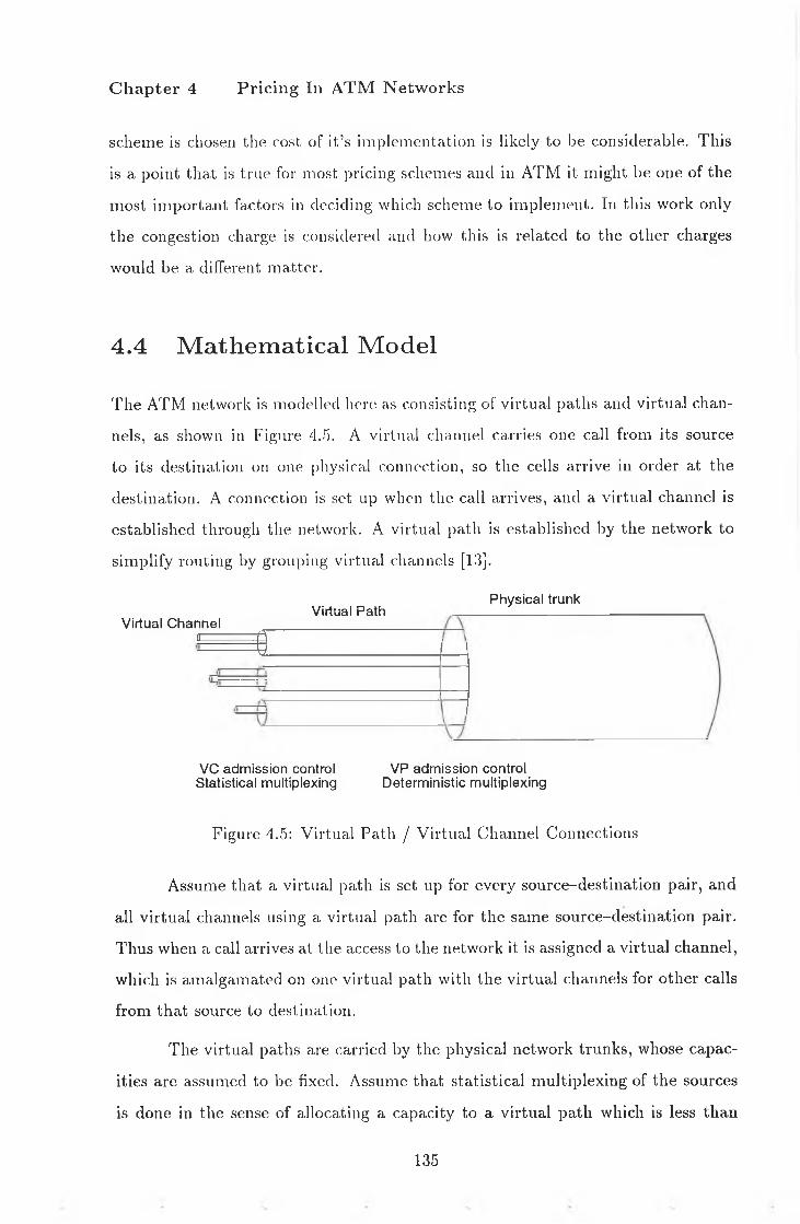
scheme is chosen the cost of i t ’s im plem entation is likely to be considerable. This is a point tha t is true for most pricing schemes and in ATM it m ight be one of the most im portan t factors in deciding which scheme to implement. In this work only the congestion charge is considered and how this is related to the o ther charges would be a different m atter.
C h a p te r 4 P r ic in g In A T M N etw o rk s
4 .4 M a th em atica l M o d elT h e ATM network is modelled here as consisting of virtual paths and v irtua l channels, as shown in Figure 4.5. A virtual channel carries one call from its source to its destination on one physical connection, so the cells arrive in order a t the destination. A connection is set up when the call arrives, and a v irtual channel is established through the network. A virtual path is established by the network to simplify routing by grouping virtual channels [13].
Physical trunkVirtual Channel
a------
Virtual Path
I
V C admission control Statistical multiplexing
VP admission control Deterministic multiplexing
Figure 4.5: V irtual P ath / V irtual Channel Connections
Assume tha t a virtual pa th is set up for every source-destination pair, and all v ir tual channels using a virtual path are for the same source-destination pair. Thus when a call arrives at the access to the network it is assigned a virtual channel, which is am algam ated on one virtual p a th with the v ir tua l channels for o ther calls from th a t source to destination.
T he virtual paths are carried by the physical network trunks, whose capacities are assumed to be fixed. Assume th a t s tatistical multiplexing of the sources is done in the sense of allocating a capacity to a virtual p a th which is less th an
135

C h a p ter 4 P r ic in g In A T M N etw o rk s
the sum of the virtual channel peak bandwiclths using this virtual path . The network decides the capacities of the virtual paths and these satisfy the physical trunk capacity constraints. For example, the network could simply do deterministic multiplexing at the virtual pa th level, as in Figure 4.5. Determ inistic multiplexing means tha t the sum of the virtual paths tha t use a physical trunk would be less than or equal to the capacity of the physical trunk . This is unlike statistical m ultiplexing where it is possible to divide more than the capacity of the physical trunks among the virtual paths. By doing deterministic multip lexing different virtual path capacities are not allowed to interact, at least not in real tim e. The virtual path capacities are assumed to be fixed. This assumption can be relaxed by having the virtual paths interact with each other at a longer t im e scale than the t im e scale of the pricing [57] w ithout affecting the model proposed.
4 .4 .1 U ser B en efit F unctionsT he users connected to an ATM switch wish to send traffic to various destinations. Their benefit versus bandw idth curve for a particu lar connection is assumed to be concave increasing in general, as shown in F igure 4.6. This follows the usual economic assumption th a t users value the first p a r t of a com m odity the most, with diminishing incremental valuation as they get more of the com modity [19, 89],
Benefit
Figure 4.6: User Benefit As A Function Of Traffic Rate
Consider the problem faced by a user a ttached to ATM node i in deciding their bandwidth dem and for a particular connection to destination ATM node j . Let the virtual p a th corresponding to this source-destination pair be denoted Vq.
136

C h a p te r 4 P r ic in g In A T M N etw o rk s
T he network quotes all users a price per unit of bandw idth 011 Vq, irq. Each user then uses their private benefit function benrq for connection r to decide their bandw idth a t th a t price, brq. This decision process can be form ulated m athem atica lly as follows :
maximise benrq(brq) — TTq ■ brq (4-2)
The user solves a maxim isation problem of this form for each connection to destination ATM node j , for each j . The optim ality condition for Equation 4.2 can be solved [49] and is given by Equation 4.3 :
dbenrq ~db, = 0 , V V, (4.3)'rq
4 .4 .2 S y stem P ro b lemConsider now the system m ade up of all the users and the ATM network, and suppose for the m om ent th a t there is a single ‘system m an ag er’ who knows all the problem data. It will be. seen th a t no such ‘system m anager’ is needed.
T he problem facing this ( hypothetical ) system m anager is to choose the bandw idth dem ands to m axim ise aggregate benefit, subject to the v ir tual pa th capacity constraints. Here the virtual path capacity constraint is replaced by a corresponding buffer capacity constraint, which ensures th a t the ATM switch buffer occupancy, denoted as bq, is less than the buffer size B q b u t allows the inpu t rates to tem porarily exceed the ou tpu t rate of the virtual pa th :
bq < B q , V Vq (4.4)
This constraint is d ropped and a barrier function te rm is added to the system objective function, B u f f costq. This function will be a convex function and the shape of this cost te rm is shown in Figure 4.7, and ensures th a t as the buffer capacity is approached, the ‘cost’ of assigning bandwidths increases to infinity.
The system problem can be formulated as follows :
maximise ^a l l V ,
^ ", benrq(brq) — B u f f c o s t q > (4-5)
137

C h a p te r 4 P r ic in g In A T M N etw o rk s
Figure 4.7: Barrier Function For q Buffer Capacity C onstraint
Because of the concave natu re of the functions defined, there is a guarantee tha t there will be an optimal solution. These optim ality conditions for the system problem are
dben rqdbrq
d B u f fc.ost.q 8ba
dbnd ( Z r brq) = 0 , V r , K (4.6)
Comparison of Equations 4.3 and 4.6 shows th a t by settingd B u f fco.stq
dbadbn
d (£r brq )(4.7)
individual user benefit maxim isation ( Equation 4.3 ) coincides with system optim ality ( Equation 4.6 ). Therefore if the network opera tor sets the prices according to Equation 4.7, the users will self-select their optim al bandw idth dem ands while com peting for the virtual pa th capacity.
One of the m ajor advantages of this scheme is th a t there is no need to have a ‘system m anager’ who knows all the user benefit functions as well as the network data . This is because the prices can be set as in Equation 4.7 by the network without any knowledge of any user benefit function. T he users will then use the price to maximise their private benefit functions and this in tu rn will give the network information to have the optim al conditions for the network. Therefore the network operator or provider can induce system -op tim al user behaviour by setting the prices as in Equation 4.7 without any knowledge of the user benefit functions.
138
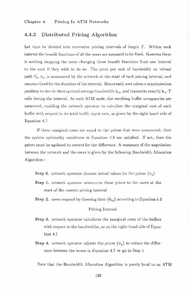
C h a p ter 4 P r ic in g In A T M N e tw o r k s
4 .4 .3 D istr ib u ted P ricin g A lgo rith mLet time be divided into successive, pricing intervals of length T . W ith in each interval the benefit functions of all the users are assumed to be fixed. However there is nothing stopping the users changing these benefit functions from one interval to the next if they wish to do so. T h e price per unit of bandwidth on virtual pa th Vq, 7T9, is announced by the network at the s ta r t of each pricing interval, and remains fixed for the duration of the interval. Hence each user solves a maxim isation problem to decide their optimal average bandw idth bTq, and transm its exactly brq'T cells during the interval. At each ATM node, the resulting buffer occupancies are measured, enabling the network operator to calculate the marginal cost of each buffer with respect to its total traffic input rate, as given by the r igh t-hand side of Equation 4.7.
If these marginal costs are equal to the prices th a t were announced, then the system optim ality conditions in E quation 4.6 are satisfied. If not, then the prices m ust be upda ted to correct for the difference. A sum m ary of the negotiation between the network and the users is given by the following Bandwidth Allocation Algorithm :
Step 0. network operator chooses initial values for the prices {7rg}Step 1 . network operator announces these prices to the users a t the
s ta r t of the current pricing intervalStep 2. users respond by choosing their {brq} according to Equation 4.3
Pricing Interval
Step 3. network operator calculates the m arginal costs of the buffers with respect to the bandwidtlis, as on the r igh t-h and side of Equation 4.7
Step 4. network operator adjusts the prices {7t9} to reduce the difference between the terms in Equation 4.7 go to Step 1
Note th a t the Bandwidth Allocation A lgorithm is purely local to an ATM
139
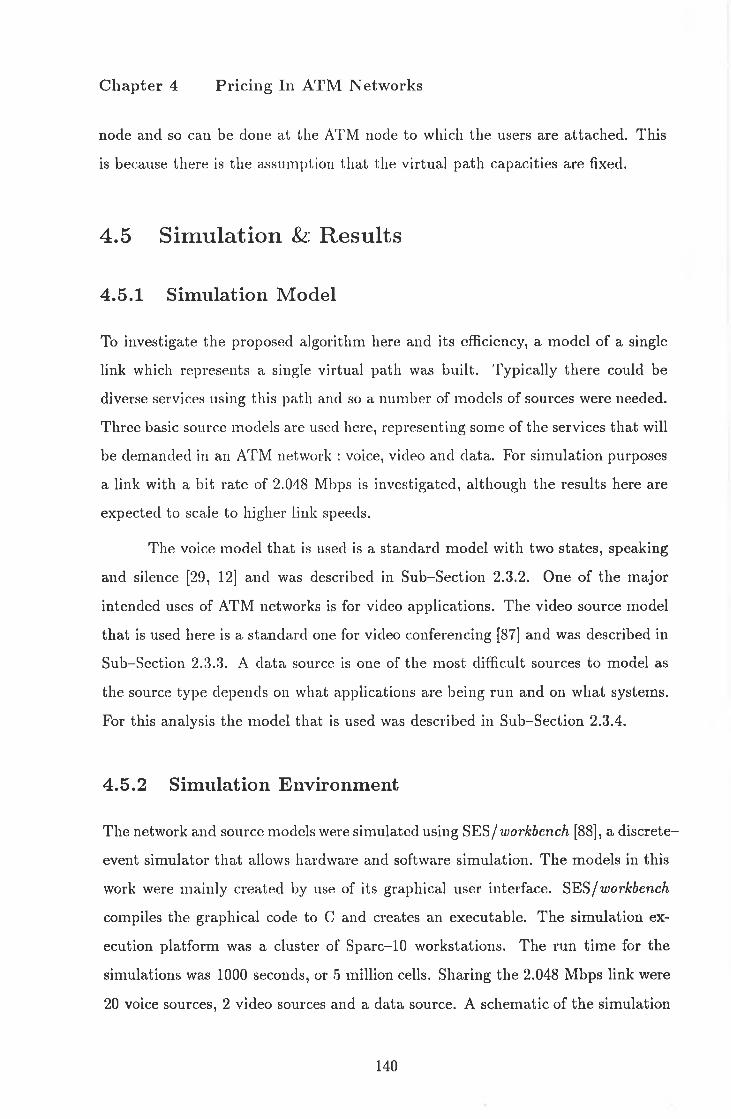
C h a p ter 4 P r ic in g In A T M N etw o rk s
node and so can be done at the ATM node to which the users are a ttached . This is because there is the assumption th a t the v irtual p a th capacities are fixed.
4.5 S im u la tion &: R esu lts
4 .5 .1 S im u lation M od elTo investigate the proposed algorithm here and its efficiency, a model of a single link which represents a single virtual p a th was built. Typically there could be diverse services using this path and so a num ber of models of sources were needed. Three basic source models are used here, representing some of the services th a t will be dem anded in an ATM network : voice, video and data . For simulation purposes a link with a b it ra te of 2.048 Mbps is investigated, although the results here are expected to scale to higher link speeds.
The voice model th a t is used is a s tandard m odel with two sta tes, speaking and silence [29, 12] and was described in Sub-Section 2.3.2. One of the m ajor intended uses of ATM networks is for video applications. The video source model th a t is used here is a s tandard one for video conferencing [87] and was described in Sub-Section 2.3.3. A d a ta source is one of the most difficult sources to model as the source type depends on what applications are being run and on what systems. For this analysis the model tha t is used was described in Sub-Section 2.3.4.
4 .5 .2 S im u lation E nvironm entThe network and source models were simulated using SES/ workbench [88], a d iscrete- event sim ulator th a t allows hardware and software simulation. T he models in this work were m ainly created by use of its graphical user interface. SES /workbench compiles the graphical code to C and creates an executable. T he simulation execution p la tform was a cluster of Sparc-10 workstations. T he ru n tim e for the simulations was 1000 seconds, or 5 million cells. Sharing the 2.048 Mbps link were 20 voice sources, 2 video sources and a da ta source. A schem atic of the simulation
140
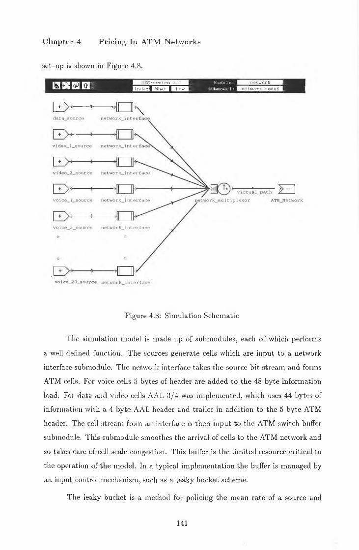
C h ap ter 4 P r ic in g In A T M N etw o rk s
se t-up is shown in Figure 4.8.
BSBB :.*Vd«8 ian 2 . 1 , 'Jo ! -,..r wr»rk 1 •rn r l^ y jj What- 1 How ■ •'!*!; • * 1 1 !)«-t W-'l k modnl |
E>— ----- *[□K
Figure 4.8: Simulation Schematic
The simulation model is m ade up of submodules, each of which performs a well defined function. T he sources generate cells which are input to a network interface submodule. T he network interface takes the source bit s tream and forms ATM cells. For voice, cells 5 bytes of header are added to the 48 byte information load. For data and video cells AAL 3 /4 was im plem ented, which uses 44 bytes of information with a 4 byte AAL header and trailer in addition to the 5 byte ATM header. The cell s tream from an interface is then inpu t to the ATM switch buffer submodule. This subm odule smoothes the arrival of cells to the ATM network and so takes care of cell scale congestion. This buffer is the lim ited resource critical to the operation of the model. In a typical im plem enta tion the buffer is m anaged by an input control mechanism, such as a leaky bucket scheme.
The leaky bucket is a m ethod for policing the m ean ra te of a source and
141

C h a p ter 4 P r ic in g In A T M N etw o rk s
still allowing bursts to occur. The mean ra te is the ra te at which tokens are given to allow cells past the network interface and into the network. If there were no storage of tokens then this would be a pure mean ra te policing function. If the source can store tokens, it could use up all the tokens in one go by bursting cells into the network. If a source has no remaining token allowance then ra the r than dropping th a t cell, it is usually marked. If there is congestion in the network and cells have to be discarded the m arked ones are discarded first. T he leaky bucket does not lower the cell loss in a buffer; it merely selects which ones to lose. The pricing scheme here actually lowers the probability of cell loss by smoothing the traffic adaptively based on the buffer occupancy to avoid congestion.
In the proposed scheme here a price is generated by the network based on the present s ta te of the network buffer, and the sources adapt their dem ands based on this. The leaky bucket can also be implemented on top of this scheme so tha t if there is cell loss the marked cell will be discarded first. T he model takes in cells over an interval of about 50 milli-seconds and gives a price to all the sources sharing the link. The price, reflects the congestion in the buffer ( if any ) and hence on the virtual path. T he higher the buffer occupancy, the higher the price sent back to the sources. For these simulations the following functions are used :
B u ! ! c o s t ' = " k (4 ,8 )
The corresponding price tha t is generated is then the solution to Equation 4.7 which is given by Equation 4.9.
7T - ---------- — — ------- (4 9)9 (B q - bqy 9 ( E r M 1 ‘ j
This price is received by the network interfaces which use it to calculate how m any cells they should input in the next interval. For example, a d a ta source may calculate tha t at the given price it should input 100 cells to the network, b u t if no cells are actually generated by the d a ta source in th a t tim e interval then obviously there is no input. The outline of the d istributed pricing algorithm th a t is used is contained in Section 4.4.3.
142

C h a p te r 4 P r ic in g In A T M N etw o rk s
In an interval of about 50 milli-seconds the link can serve about 250 cells and the buffer size tha t is choosen is 250 cells. This means tha t when the buffer is full there should be no more than 250 input cells over the next interval. The input sources are shaped as much as possible by the tim e the cells are form ed at the network interfaces, so the cells arrive approxim ately equally spaced in tim e. It is s tandard to give guarantees to rea l- t im e services, th a t if their cells get through, then the m axim um access delay they experience is the buffer queueing delay, which in this case is small ( 50 milli-seconds ).
4 .5 .3 R esu ltsIn practice voice and video calls may be inflexible with respect to bandw idth , and even if they are flexible they do not perm it a huge statistical multiplexing gain ( except for the enhancement layer of a two layer codec ) compared to data . In these, simulations here the. assumption is th a t the voice and video have inflexible bandwidth demands. There are 20 voice sources which have a combined m ean of 492 kbps and a potential m axim um of 1413 kbps. T he video has two channels, both one layer codecs, with a combined m ean of 507 kbps and a potential m ax im um of 1773 kbps. Even without a data source there is clearly a non zero probability of cell loss. The d a ta source has a mean of 237 kbps and a potential m ax im um equal to the bit ra te of the link, 2048 kbps.
The results of the simulations are sum m arised in Table 4.4 for the two cases of no pricing used and the pricing scheme proposed here used.
When a leaky bucket scheme alone was implemented the results in Figure 4.9.A were obtained for the sampled buffer occupancy. In Figure 4.9.B the plot of buffer occupancy is shown over the interval when the pricing scheme here was used. The buffer is not as occupied as in Figure 4.9.A . This is apparent when the loss probabilities are compared.
The pricing scheme produced no cell loss, e ither of m arked or unm arked cells2. There is a small decrease in the quality of service provided to the da ta
2It should be noted that there could be cell loss if a longer interval was chosen.
143

Table 4.4: Results For Both No Pricing & Pricing
C h a p ter 4 P r ic in g In A T M N e tw o r k s
N o p r i c in g u s e dTotal num ber of cells generated 2,914,191N um ber of m arked cells lost 32,268N um ber of unm arked cells lost 191,044Percentage of cells lost 7.7%P r i c i n g u s e d N o ce ll loss
Number of cells
A. W ithou t PricingNumber of cells
B. W ith Pricing
Figure 4.9: Buffer Occupancy W ith And W ithou t Pricing
source to gain this improvement. Figure 4.10 A shows the sampled num ber of
144

C h a p ter 4 P r ic in g In A T M N etw o rk s
waiting d a ta cells of d a ta over the interval when the leaky bucket is used. By comparing Figure 4.10 A to Figure 4.10 B for the pricing scheme, it can be seen th a t the m ean waiting tim e for the d a ta source has increased.
Number of cells x 1(P
15.00_
10.00 .
5.00.
0.00.0.00
Number of cells x 103
15.00_
10.00.
5.00.
0.00.
j J L0.20 0.40 0.60 0.80
A. W ithou t Pricing1.00
Time, sec x 10
i L lT0.00 0.20 0.40 0.60 0.80
B. W ith Pricing
y j1.00 lim e, sec x 10
Figure 4.10: Delay, In Cell Times, For D ata Cells W ith And W ithou t Pricing
145

C h a p ter 4 P r ic in g In A T M N etw o rk s
4.6 Im p lem en ta tion O f A P r ic in g S ch em eT he possible implementation of any pricing scheme involves m any practical difficulties, such as the volume of da ta to store, where to store the d a ta and security of the data. W ith usage based pricing, as presented here, there are additional problems associated with the measuring and recording of the usage and hence charge to be m ade to a user. A simplification is m ade here th a t it will be possible to implement the pricing at the edge of the network, instead of say within the network as in a hop-by-hop or segm ent-by-segm ent fashion. The proposed se t-u p could look like th a t shown in Figure 4.11.Users
Access Switch
Figure 4.11: E n d -T o-E n d Im plem entation Of A Pricing Scheme
4 .6 .1 G eneration O f T h e P riceThe measure of congestion tha t is used to determ ine the price from the network is the buffer occupancy. The buffer in question is the buffer for the v ir tual pa th tha t the connection is carried on from the access switch. Therefore all connections tha t are using the same virtual path a t the access switch will get the same price from the network. It is implicit tha t with the above assumptions th a t the congestion of the connections using the same virtual pa th will be similar. However it is possible th a t this may not be the case and so o ther virtual pa ths tha t are concatenated to the first virtual pa th may have to signal back across the network to the access switch what their s ta te of congestion is.
The buffer occupancy could be measured and averaged over a num ber of
146

C h a p te r 4 P r ic in g In A T M N etw o rk s
cell times, or it could be a moving average, again over a num ber of cell times. However what it imagined here is th a t the instantaneous cell occupancy at every pricing interval is used to calculate the price. W ith in a switch this would m ean th a t each v irtual path would need to calculate the price from its buffer occupancy every pricing interval. However it would be possible to stagger the measurem ents and calculations so tha t they do not occur together and impose a load on the switch processor.
4 .6 .2 P rice P assin g From N etw ork To U serTo pass the price information from the switch to the users is one of the most difficult issues. One possible suggestion is to pass the price back to the users by means of a specially dedicated operations and maintenance, (OAM), cell. If the pricing interval is small, for example 1.7 milli-seconds, then there are 600 OAM cells generated per second, which equals a b it ra te of 254.4 kbps. This m ay not seem excessive, bu t this would be for every connection tha t is connected to the switch. So if you had relatively small b it ra te connections, for example sub-M bps connections, then the overhead would be excessive. It m ight instead be possible to pass the price back through an OAM cell to each device connected to the switch and then let each device use th a t price to control all of i t ’s connections. This would be helpful especially for d a ta communications, as it is possible th a t a single processor could control multiple connections, some of which might be dorm ant on the second tim e scale.
Another possibility is to try not to generate an OAM cell for each price bu t ra the r to pass the price back to the users within other cells tha t are flowing in the reverse direction. The price th a t is generated could more than likely be encoded with 2 bytes of code, i.e., there would be at most a choice of 65,536 different prices in to ta l throughout the network. This seems a reasonable num ber when consideration is given to the fact tha t the price is based on the buffer occupancy and so there are unlikely to be more than 65,536 different levels of buffer occupancy, or 65,536 cells in a buffer. Therefore the 2 byte price would be em bedded in an reverse cell to the user from the access switch. R a th e r than try and use a complicated m ethod
147
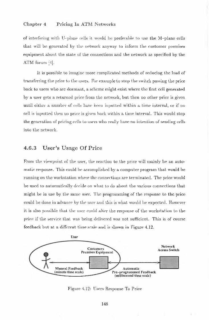
C h a p ter 4 P r ic in g In A T M N etw o rk s
of interfering with U -plane cells it would be preferable to use the M -p lane cells tha t will be generated by the network anyway to inform the custom er premises equipm ent abou t the s ta te of the connections and the network as specified by the ATM forum [4].
It is possible to imagine more complicated m ethods of reducing the load of transferring the price to the users. For example to stop the switch passing the price back to users who are dorm ant, a scheme might exist where the first cell generated by a user gets a returned price from the network, b u t then no o ther price is given until either a num ber of cells have been inputted within a t im e interval, or if no cell is inpu tted then no price is given back within a t im e interval. This would stop the generation of pricing cells to users who really have no intention of sending cells into the network.
4 .6 .3 U se r ’s U sa ge O f P riceFrom the viewpoint of the user, the reaction to the price will m ainly be an autom atic response. This could be accomplished by a com puter program th a t would be running on the workstation where the connections are term ina ted . T he price would be used to autom atically decide on what to do about the various connections tha t might be in use by the same user. T he program ming of the response to the price could be done in advance by the user and this is what would be expected. However it is also possible tha t the user could alter the response of the workstation to the price if the service tha t was being delivered was not sufficient. This is of course feedback bu t a t a different t im e scale and is shown in Figure 4.12.
Customers \ Premises Equipment
Manual Feedback (minute time scale)
User
Automatic Pre-programmed Feedback
(millisecond time scalc)
Network Access Switch
Figure 4.12: Users Response To Price
148

C h a p ter 4 P r ic in g In A T M N etw o rk s
The program ming of the intelligent interface to handle the price can be also customised to allow for the user to change the overall performance, without going into the details of pricing scheme, by application program s th a t could be written for interfacing with it.
4.7 D ifferent T y p es O f E fficien cies In N etw orksIn focusing on user preferences, two very different notions of efficiency need to be distinguished :
• N e t w o r k e ff ic ien cy refers to the utilisation of network resources such as bandwidth and buffer space.
• E c o n o m ic e ff ic ien cy refers to the relative valuations the users a ttach to their network service.
If a network can maintain an acceptable level of service over t im e while minimising the resources necessary to provide this service, its operation is ( network ) efficient. If users who value network service more are served ahead of users who value it less, then tha t operation is ( economically ) efficient.
Feedback signals from the network can help to increase bo th types of efficiency. When the network is heavily loaded, users who are flexible about when they input traffic, can be signalled to wait; when the network is lightly loaded again these flexible users can be encouraged to transm it. In this way m any of the congestion problems tha t can occur if the offered load is regarded as fixed can be avoided. The flexible users absorb the longer delays and do not tie up network resources, which can therefore be used to serve less flexible users.
A cost measure can be defined for any level of network operation. Typically this cost is made up of several components corresponding to fixed ( sunk ) costs, variable operational costs, and so on. One crucial com ponent is the congestion cost: the cost imposed on other users when a par ticu la r user adds traffic tha t increases network congestion ( degrades service quality ). If the prices quoted to
149
C h a p te r 4 P r ic in g In A T M N etw o rk s
the users reflect the current costs of operating the network, then those users who value network service more will choose to transm it, and users who value it less will wait for lower prices. If the network is lightly loaded then the prices will be close to zero and all users can be accommodated.
These increases in efficiency ( of either type ) require flexible or p rice- sensitive users to be more closely involved in controlling their connections than is currently the case. Not all users are capable of, or want to be involved in, dynamically adjusting their traffic inputs. How the network owner wishes to differentiate between these user preferences is not of concern here ( for example, by offering a “discount” to flexible users, or charging “p rem ium ” prices to users who want a predeterm ined price at connection se t-up ).
4 .7 .1 E conom ic Fram ew orkIn this Sub-Section one possible m ethod for com puting adaptive prices is shown. The users discussed below are thus adaptive users ( either adaptive best-effort, inelastic, or elastic. ). A more detailed description can be found in [56, 57]. O ther pricing schemes for com m unication networks have been suggested, e.g. [48, 51].
The network and its users are considered to form an economy or economic system. The system has various resources such as link bandwidths and buffer spaces th a t can be used to meet user dem ands for service. Network constraints such as buffer sizes or link capacities are translated into cost functions on the dem ands for resources. This reflects the fact tha t one user’s consumption of bandw idth or buffer space gives rise to a “cost” ( in terms of longer delays, less available bandwidth , longer buffer occupancies, etc ) which is borne by all users.
Each adaptive user is viewed as placing a benefit, or willingness-to-pay, on the resources they are allocated. Given a price per unit of bandw idth or buffer space, a user’s benefit function completely determines th a t user’s traffic input. A benefit function could follow the usual economic assum ption of diminishing increm enta l benefit as more of the resource is consumed ( Figure 4.13(a) ). Or it could be a simple threshold rule, or series of threshold rules, for deciding how much of
150

C h a p te r 4 P r ic in g In A T M N etw o rk s
the resource to request based on the current price ( Figure 4 .13(b),(c) ). Users are allowed to change their benefit functions every feedback interval so the examples in Figure 4.13 are for a particular interval.
Bandwidth
benefit bandwidth
A
bandwii3?h
( b )pri!ce
benefit bandwidth
Figure 4.13: Possible User Benefit Functions
The network operator sets the prices so th a t the marginal benefit the users place on their resource allocation is equal to the m arginal cost of handling the resulting traffic in the network3. The basic requirem ent is tha t price should go to infinity as usage of the resource approaches capacity. T he network operator dynamically adjusts the prices based on current network conditions. It tu rns out th a t it is not necessary for the network operator to know the user benefit functions; therefore this pricing scheme is suitable for both public and private networks.
4 .7 .2 U sers M odelsIn Sub-Section 4.2.3 the possible types of users were discussed. In this Sub-Section the e la s t i c and in e la s t i c users are modelled. T he users have a certain file size to send over a num ber of pricing intervals and what has to be decided is how much to
3These prices only address the variable costs corresponding to network constraints.
151

C h a p ter 4 P r ic in g In A T M N etw o rk s
send in each interval if any at all, based on the price th a t is given from the network.
4 .7 . 2 . 1 E la s t i c U s e r
There is one essential element to preferences for elastic traffic which is tha t the traffic has value even if it experiences delay. As shown before, however, the value should be declining the longer is the delay ( if it isn’t, then the decision rule to send is simple : never send unless the price is zero, or the lower bound, if not zero ). Another characteristic tha t is not necessarily intrinsic to all elastic traffic, bu t seems to be characteristic of most types ( e.g., files, messages ), is tha t a transfer has zero value unless the entire message ( file ) is delivered.
At the s ta rt of the connection for the elastic user, the user guesses the average price and the average Peak Cell R ate ( P C R ) over the lifetime of the connection and these are denoted by P* and P C R * respectively. These could be based on past experience or be given by the network. Assume th a t P* > 0 and P C R * > 0. Assume also th a t the connection lifetime is long with respect to the pricing interval. This will avoid the idea of the end effects th a t might influence the decision of the user, and they will always be willing to wait if the decision is not to send now. Assume tha t the users think th a t the price in the next interval will go directly to the average in the next interval, regardless of the actual price now. This is the simplest possible forecasting of the user. T he benefit th a t the user places on the connection is as follows :
b e n { x ,v } = v — h(d) (4-10)
T he value tha t the user places on the file size x cells is given by v if it were delivered without delay. When a delay of d occurs to the finish then the penalty of h(d) is paid in terms of lost benefit. The elastic user is flexible with respect to delay and so the send decision involves time, in particular their e s tim ate of the effect on overall delay of sending some cells now, as allowed by their current PCR . In general there is a recursive decision making process where e ither send at current P C R k o r wait till next interval, where: send at current PCRk+i o r wait till next interval, where: send at current P C R k + 2 ° r wait till next interval, etc.
152

C h a p ter 4 P r ic in g In A T M N etw o rk s
The model for the delay cost for the user, li(d), would have the following a ttr ibu tes : h (0) = 0; /;.(oo) = v. An example of this could be a function tha tapproaches v asym ptotically like h(d) — ?;(! — e~d) which is shown in F igure 4.14.
h(d)
Figure 4.14: Possible User Delay Cost Function
The elastic, user will decide whether to send or not in the next interval based on the fact of whether i t ’s b e t te r to wait till the next interval to send, or if i t ’sworth sending anything at all. Suppose tha t the length of the interval is given bytint and tha t the user has already paid the am ount already-charged{t) and tha t the current price is Pt and the allowable peak cell ra te from the network is P C R t- There will be a num ber of cells remaining to be sent from the elastic user and this is given by X ji( t) which is less than A'. There can be two cases as follows :
1 . In this case the user can finish the whole message in the interval, so the decision to send is based on if i t ’s b e t te r to wait till the next interval to send or not. Of course the user may have run out of t im e and have to drop themessage with no benefit at all. P C Rt £;„( > X n ( t )
2. In this case, the user can not finish the whole message in the interval, so the decision to send is based on maybe being able to send at the average rates in future intervals as well. P C R t tint < X n {t)
153

C h a p ter 4 P r ic in g In A T M N etw o rk s
C ase 1
In this case if the user sends now the benefit is :
b en e fi t = v — h(t) — already-charged(t) — Pt X R(t) (4-11)
However if the user sends nothing in the interval then there will be X R (t) left to be sent in the next interval. This will take a more intervals to com plete in the forecasted version from the user, where :
X p ( t )a = P C R * t iniT he benefit tha t the user expects to get would then be :
(4.12)
benefit, = v — h(t + a ) — already-c.harged(t) — P* X R(t) (4-13)
Comparing Equation 4 .1 1 and Equation 4.13, the user will send n o w iff :
h(t + a) - h(t) + ( P * ~ Pt ) X R(t) > 0 (4.14)
This means tha t the benefit of waiting and getting the average price and P C R will not be worth the delay in sending. Otherwise the user will wait and send nothing in the interval t.
C ase 2
In this case the user can’t finish the message in the interval t due to the length of the message left and the P C R available from the network. B u t the user can send the m axim um possible now or wait till the next interval. If the user sends the m axim um in this interval then there will be X R(t + 1) cells rem aining at the end of the interval t where :
X R(t + 1 ) = X R(t) - P C R , t int (4.15)
T he expected benefit to the user of sending the cells now would be :
b en e fi t = v — h(t + (3) — already-charged{t)- Pt P C R t t in t - P* X R{t + 1) (4.16)
154
C h a p ter 4 P r ic in g In A T M N etw o rk s
where /? is the expected num ber of more intervals th a t the user will need to send the remaining cells after this interval and is given by :
X R(t + 1) P C R * t inl (4.17)
Now by sending nothing now it will take a more intervals to send the message, where a is as before. The expected benefit to the user of waiting until after this interval to send anything would be :
b en e f i t — v — h(i. + o') — already-charged{t) — P* X R(t) (4-18)
Comparing Equation 4.16 and Equation 4.18, the user will send n o w iff :
h (t + a ) - h{t + ft) + (P* - Pt) P C R , t inl > 0 (4.19)
Otherwise the user will wait and send nothing in the interval t.
So in sum m ary the elastic user acts as follows :
h(t + a ) ~ h{t) + {P* - Pt) X R(t) > 0 , for P C R t t int > X R(t)h(t + a) - h{t + {3) + ( P * - Pt ) P C R t Um > 0 , for P C R t t int < X R(t)
Otherwise wait and send nothing in interval t.
4 .7 .2 .2 I n e l a s t i c U s e r
This user has a delay bound on the traffic, b u t can tolerate only sending a fraction of the cells tha t are ready to go in the interval in question. Assume th a t if they are not sent in the interval then there are discarded and useless to the user. This might be like the second layer of a video codec, which only enhances the picture, b u t are useless if they arrive after the fram e has been shown. Assume th a t the user has a concave benefit function, b e n e f i t ( X ) , on the num ber of cells sent, X . This is fixed for each interval b u t might vary from one interval to another or be fixed. If the user sends in interval t the num ber of cells X t then the benefit to the user
155
C h a p ter 4 P r ic in g In A T M N etw o rk s
is b e n e f i t t( X t ). How the user decides 011 the num ber of cells to send in interval t depends on the price given to the user Pt . T he user solves the following problem :
= P> (4.20)(JA
The user then solves for X and this value is the num ber of cells X t sent in the interval t.
4.7 .3 A n oth er D istr ib u ted P ricin g A lgorith mA distributed iterative pricing algorithm has been developed [56]. The d is tributed natu re of the pricing algorithm suggests tha t it m ay be possible to meet the realtim e feedback requirement. In addition, the com putation required per iteration at each user and ATM access switch is simple, which suggests th a t inexpensive processing elements may be sufficient in executing the algorithm.
In a feedback-based fast reservation scheme, it m ay be necessary to enforce the user requests to avoid unnecessarily blocking o ther users. One suggestion to provide financial incentives to users to encourage tru thfu l traffic descriptors ( for both adaptive and non-adaptive users ) was presented in [40]. In the scheme shown in Figure 4.15, the network operator could charge each elastic, user according to their request if their actual cell input is less than tha t .
It is possible to extend the pricing algorithm of Figure 4.15 to include the adjustm ent of V P capacities using a similar iterative, scheme. T he V P adjustm ents are not purely local, since contention between users is not confined to the network access points as before. On the other hand the V P adjustm ents have a longer tim e period in which to carry out their com putations.
4 .7 .4 S im ulation D eta ilsThe simulation details are similar to those discussed in Sub-Section 4.5.2. In the proposed scheme here a price is generated by the network based on the present sta te of the network buffer, and all the sources adap t their dem ands based on this.
156

C h a p ter 4 P r ic in g In A T M N etw o rk s
Figure 4.15: D istributed Iterative Pricing Algorithm
W hat is proposed and simulated here adheres to the UNI 3.0 specification from the ATM Forum [4]. A leaky bucket can also be im plem ented on top of the scheme here so tha t if there is cell loss it is possible to discard the m arked cells first.
The model takes in cells over a pricing interval and gives a price to all the sources sharing the link. The price reflects the congestion ( if any ) in the buffer and hence on the virtual path. T he pricing interval is short com pared to the video frame time : a value of about 0.05 of a fram e tim e was chosen. To achieve feasible run times cell scale effects are neglected. This neglecting of cell scale effects is critical to the speed up of the simulations. T he to ta l utilisation of the link is then high, at a value of around 0.85. It is possible to com pare the performance of the pricing scheme to o ther access control schemes by looking a t the loss and at the value of the traffic carried.
The initial set up is a high speed ATM 155 Mbps link with two types of users
157
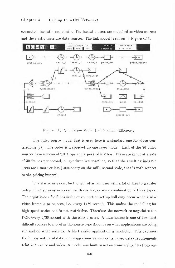
C h a p ter 4 P r ic in g In A T M N etw o rk s
connected, inelastic and elastic. The inelastic users are modelled as video sources and the elastic users are da ta sources. T he link model is shown in Figure 4.16.
r./r|*»s io n 2 . 1 M o d u le : sim p r i c eWM* 1 H***w j S u b m o d e l: l i n k mnrip 1
E>p r i c e _ s t a r t s m a l l _ i s m a l l _ 2 i n t e r _ 2 p r i c e _ s e t p r i c e _ f i n i s h
Figure 4.16: Simulation Model For Economic Efficiency
The video source model tha t is used here is a standard one for video conferencing [87]. The codec is a speeded up one layer model. Each of the 20 video sources have a mean of 2.3 Mbps and a peak of 5 Mbps. These are input a t a rate of 30 frames per second, all synchronised together, so tha t the resulting inelastic users are ( more or less ) s ta tionary on the milli-seconcl scale, th a t is w ith respect to the pricing interval.
The elastic users can be thought of as one user with a lot of files to transfer independently, m any users each with one file, or some combination of these types. T he negotiations for file transfer or connection set up will only occur when a new video frame is to be sent, i.e. every 1/30 second. This makes the modelling for high speed easier and is not restrictive. Therefore the network re-negotiates the P C R every 1/30 second with the elastic users. A d a ta source is one of the most difficult sources to model as the source type depends on what applications are being run and on what systems. A file transfer application is modelled. This captures the bursty natu re of d a ta communications as well as its looser delay requirements relative to voice and video. A model was built based on transferring files from one
158

C h a p te r 4 P r ic in g In A T M N etw o rk s
com puter to another. An empirical d istribution for file size ranges was obtained from actual files stored on one of the com puters in DCU. In the simulations a range was chosen according to this empirical distribution , and then a file size was chosen from a uniform distribution within this range. The am ount of d a ta transfer can be varied depending on how many files are to be transferred. The p e a k - to -m e an ratio of this source can be high with values up around 1000. There are on average 20 d a ta sources in use and these are taken from a uniform distribution between 1 and 39 sources. Each file to be sent is also taken from a uniform distribution between 20 and 660 cells. Therefore the average bit rate of a single d a ta source is about 4.3 Mbps.
The simulation was speeded up by use of tim e stepping, where the tim e step was chosen to be the frame time. This was possible as everything was known at the sta rt of the frame time, except the pricing, bu t if the price was low and the link un-congested then the pricing could be skipped. There was also an approxim ation to the price tha t the network generated. If Equation 4.8 is com puted on the cell level then the price generated will be between 0 and 1 for all values of bq < B q but when bq = B q then the price given by the network is oo. To avoid this problem the equation is changed slightly to give Equation 4.21 :
= e„ _ \ + i - bTTT ( 4 ' 2 1 )
The next detail is how to calculate the peak cell ra te th a t the network allows the elastic users. This is calculated based on the current level of the buffer and the num ber th a t can be served in an interval. If the buffer is em pty then it is desirable th a t the P C R to be equal to the num ber th a t can be served in an interval, and then find out how many active sources there are and divide th a t am ount up equally into all of them . However when the buffer s tarts to fill it is desirable to not only reduce the P C R bu t also to clear the buffer. To do this subtrac t the num ber in the buffer multiplied by 1.5 from the total num ber tha t can be served. This is shown in Equation 4.22 :
Dri D num ber tha t can be served — 1.5 bq ^ on\-T O it j or each source = Z (4.Z.Z)n um ber o j active sources
159

C h a p ter 4 P r ic in g In A T M N e tw o r k s
There is the possibility of oscillation in the price and this can be tuned by changing Equation 4.22. The average price, P*, th a t the user thinks th a t they will get from the network and the average peak cell rate, P C R *, are given by :
P* = 0.98 P* + 0.02 P P C R * = P C R (4.23)
In the simulations here, resource costs were chosen as barrier functions [49] to give a smooth increase as resource usage approached its limit. T he simulations were carried out for 20 seconds of real time, which translates into 7.3 million cell times.
4 .7 .5 R esu ltsThe results in Table. 4.5 show the difference between using adaptive pricing and no pricing at all. W hat can be seen is th a t both the network efficiency and the
Table 4.5: Results Of Both Network And Economic Efficiency
Source Type. % Loss User Value % Dec. Loss % Inc. Value
UnpricedInelastic 0 240
9 1 .0 14.8
Elastic 30.4 146Combined 19.1 386
PricedInelastic 4.4 239Elastic 0.1 204Combined 1.7 443
economic efficiency can increase by using pricing at the same time. Here there was an increase of 14.8% in the ecouomic benefit to the users as well as a decrease of 91% in the num ber of cells lost.
4.8 H ow P ric in g F its In to T h e A T M C ontrolsThere are two m ain functions in the area of congestion and control of ATM sources, namely connection admission control, ( CAC ), and usage param ete r control,
160

C h a p te r 4 P r ic in g In A T M N etw o rk s
( U PC ), as is shown in Figure 4.17. ATM is connection based and the understanding is th a t each connection will be able to describe itself and will require a certain quality of service, ( QOS ). The description of the connection will be by using some param eters tha t are useful to the network in deciding if it will accept the connection into the network and give it the required QOS while still m aintaining the QOS to all the other connections in the network. Therefore the CAC problem is multilevel and distributed across the whole network. Many methods have been proposed to break this problem into smaller more manageable ones. T he most promising solution is tha t proposed by effective bandwidths ( see Sub- Section 1.5.3 ) which effectively describe a connection independently of the other connections sharing the network and so decouples the problem. There is a further advantage of effective bandwidths in tha t the constraint on the network resources is linear in the effective bandwidths.
Connection Acceptance Connection In ServiceM ethod
C A C
Pricinglimited C A C
U P C
*- lim ited U P C
Figure 4.17: CAC, UPC Pricing
T he overall picture of the ATM admission scheme and congestion control might be as follows. The various sources like voice and video th a t are compressed and variable bit ra te would have an associated effective bandw idth and would be adm itted based on a CAC and then policed by a leaky bucket scheme to ensure compliance with the contract. These sources should efficiently add together to give network efficiency. The constant bit ra te sources would similarly be adm itted to the network by a CAC and be policed. However there are a num ber of sources th a t will not be able to undergo the above schemes. T h e source th a t is in mind is
161

C h a p te r 4 P r ic in g In A T M N etw o rk s
th a t of a da ta connection where there may be no description in advance in term s of effective bandwidth and so it may not be possible to include the above connection in this scheme. The other type of source is tha t of an adaptive source, where it is possible for the source to adapt i t ’s behaviour to network or other conditions without degrading the QOS of the connection. This is shown in Figure 4.18.
voicevideo } effective B W ’s, V B R -R T
data CBRdata ~ — — ■ — UBRadaptive
data ) ABR
V B R -R T variable bit rate; CBR constant bit rate; U BR unspecified bit rate; A BR available bit rate
Figure 4.18: W hich Sources Pricing Applies To
Pricing would be affected by the CAC and U PC functions of the network. It is possible tha t the CAC would limit the num ber of adaptive sources into the network, or similarly the CAC would take into account how m any priced source were adm itted , but this is not necessary for the scheme to work effectively. A lim ited CAC might be to impose a peak cell rate, ( P C R ), on the adaptive sources adm itted . There might also be a l im ited am ount of U PC on these sources then to ensure tha t they comply with this PCR . The cells from the priced sources might be policed to ensure th a t they are low priority and hence would not interfere with the other cells tha t have been given guarantees by the network.
4.9 D iscu ssionThis chapter found tha t there is a class of users, called adaptive users, th a t m ay require guarantees from the networks and this may be possible by allowing the users and network to co-operate. This chapter suggests pricing and user self-regulation
162

C h a p te r 4 P r ic in g In A T M N etw o rk s
as a means of allocating bandw idth in ATM networks. The pricing scheme is independent of the traffic, arrival model and does not require the network to police and enforce user com m itm ents in rea l- t im e as cells arrive from the sources. The pricing algorithm is d istributed and local to the ATM access nodes, suggesting th a t it may be able to m eet the tight tim e requirements of an admission control scheme. There is no need for the network to define and support traffic classes. The users have more flexible access to network resources than in other CAC schemes, bu t they take the responsibility of determining how much network resources to acquire in order to meet their par ticu lar needs. It should be noted tha t this view of th e user-network relationship should not be judged based on the feasibility or otherwise of the pricing scheme here. O ther CAC schemes may also be suitable and it remains to be seen whether the scheme, here is com patible with other approaches, perhaps in a multi-level solution approach. Similarly the pricing scheme here offers users the possibility of taking more control over their service than they have under traditional system models, bu t it does not require them to. Users whose applications have inflexible bandwidth dem ands, or who set a threshold price above which they dem and zero bandw idth , can be accom m odated in this formulation. In order to pursue an inflexible strategy, users m ay have to pay prem ium prices at times of heavy demand; but it is believed here tha t simply being forced to examine the relative im portance of their usage will give rise to a variation in user valuations th a t a scheme like ours can exploit. The success of this approach here depends on having a sufficient num ber and range of flexible applications, although how much is enough is as yet unknown.
It has also been shown th a t it is possible to maximise both the network and economic efficiency of the network at the same time. However it is felt here tha t it is still possible to use economics in networks even if it is not par t of a pricing scheme, for example in a private network. In a V PN pricing can be used to choose the desired application mix and vary this mix dynamically, as dem onstra ted in a simple case by the results here. Another use of pricing is in selectively dropping cells during congestion. Suppose th a t an application uses E therne t frames and one cell is dropped from a frame. Then the benefit of the rest of the frame should be
163
C h a p te r 4 P r ic in g In A T M N etw o rk s
set to zero if the whole frame has to be re transm itted . Similarly, if there are a num ber of video rails in progress, it may be b e t te r to drop all the cells from one connection during congestion ra ther than to spread out the loss. The feasibility of using this pricing approach here as a dynamic adaptive priority scheme in this way is one avenue for further research.
The pricing scheme here also applies to general ATM networks in which the user benefit functions are unknown to the network operator. There are m any issues which would have to be resolved in a practical im plem entation . For example, the assum ption here is tha t the benefit of making a connection is associated entirely with the sender. But in practice the benefit is shared, and some pre-connection negotiation may be necessary to agree 011 connection param eters acceptable to all parties. If interm ediate ATM nodes switch 011 the V CI as well as on the V P I [20], users a t different ATM nodes have to compete for shared resources, which complicates the algorithm and may increase the m in im um length of a pricing interval. W hether the prices used in the scheme here could be used as par t of an ATM network tariff is not clear. However it is believed here th a t the paradigm suggested is an interesting one. and may be helpful in solving these difficult network m anagem ent problems.
It has been shown here tha t pricing - and feedback in general - may be useful in resource allocation and congestion control for in tegrated-services networks. At the very least, such mechanisms deserve to be investigated : as an a lternative to m ore “trad itional” allocation and control m echanisms, or in tan dem with them .
164

Chapter 5
Conclusions
There are a num ber of conclusions tha t can be drawn from the resource allocation m ethods in ATM networks tha t have been discussed here. The issues involved in modelling and simulation were presented in C hap ter 2. There are multiple levels of resource allocation in ATM networks bu t the two th a t have been discussed here are the cell level, in C hap ter 3, and the connection level, in C hap ter 4.
After studying various m ethods of modelling and simulation techniques in Chapter 2, and why these are im portan t in ATM, it is seen tha t there is a need to present specialised models for ATM network performance. These specialised models are needed both to speed up the simulations and to decrease the num ber of simultaneous events taking place in the model. Speed up factors of over 6000 have been achieved in the satellite simulation in C hap ter 3 which was achieved by careful design of the problem being pursued and taking into account the decomposition m ethods as well as the cell ra te and s te p -b y -s te p methods. The end results are simplified approxim ate models for perform ance analysis th a t have been implemented and th a t are verified, validated and credible to the user.
At the cell level it has been shown tha t the way th a t the cells are pu t together and also the order and tim ing between them are im portan t considerations in some cases, as discussed in C hap ter 3. The way the cell is formed for an application is the ATM adap ta tion layer, ( AAL ) and for satellite links there are problems when using the AALs th a t have been standardised so far. T he problems are in terms of error correction, error detection, the percentage throughput and the m axim um
165

C h a p te r 5 C o n c lu s io n s
throughput. In C hap ter 3 after analysing and modelling the errors on the satellite links in the Deep Space Network a new AAL is proposed to allow d a ta transmission th a t incorporates selective retransmission techniques. This new AAL allows both d a ta to be guaranteed delivery, even with errors, and also improves the efficiency of the AAL by 7 .5 % over the AAL 3/4. The order and the tim ing of the cells is also shown to be im portan t when looking at the performance of the connection policer called the leaky bucket in C hap ter 3. The issue of the worst case traffic from a num ber of sources using the leaky bucket is an open problem. It was believed tha t the greedy on-off source was the worst case, even for two identical sources. It is shown in Chapter 3 th a t neither of the two traditional worst case sources produces the highest cell loss all the time. There may be of course an as yet unknown source th a t is worst case over all perm utations of the sources.
The connection level resource allocation issues are presented in C hap ter 4. It is shown tha t there is a need to have a new class of user called an adaptive user. This comes about because some users will not be catered for properly when looking at the current connection admission control schemes. There is a gap in user types when it is either not possible to describe the source or if it is possible to adap t the behaviour of the source autom atically or very quickly. The possible types of users are categorised in term s of :
1 . the ability to provide a traffic description tha t is useful to the network
2 . the need for guarantees in term s of loss and / or delay
3. whether the source is adaptive or not.
T he adaptation can be either in term s of delay or loss. After considering this, it is then possible to give sources tha t do not have a traffic descriptor guarantees on their connection, while still providing all the previously held guarantees and contracts of the other users.
There is a proposal also on how to achieve this adap ta tion in C hap ter 4. It is shown both tha t there is nothing inherently m onetary in applying economic principles to networks and th a t a possible feedback signal for adaptive users is price.
166

C h a p te r 5 C on clu s ion s
A m athem atical model is proposed for pricing, in which the congestion problem is tu rned into a constrained optimisation problem. It is then found th a t by the users acting independently, bu t optimising their benefits from the network, th a t the system optimisation is achieved. There is therefore no need for a system m anager or overseer of the network, all the network has to calculate is the price to give the user, and this is found form the constraint of the resources. By using the results from C hapter 2 it is possible to carry out simulations. T he results show th a t with pricing the cell loss is reduced and the buffer occupancy is also reduced. W ithou t pricing there was over 7% cell loss and th a t with pricing there was no cell loss.
In C hapter 4 it is also shown how a pricing scheme could be implemented and what issues need addressing. A more detailed exam ination of efficiency is carried out with the conclusion tha t there are two types of efficiencies :
1 . network efficiency
2 . economic efficiency
There is a detailed m athem atica l model of the different types of expected adaptive users, where the adapta tion can be either by tim e or by loss. A framework for the pricing and the effect on the efficiencies is formulated. By simulation it is possible to examine the effect of pricing on the different types of efficiencies. T he conclusion is th a t it is possible to increase both the economic, and network efficiency at the same tim e by using pricing. By using pricing a 9 1 % decrease in cell loss and also a 14 .8 % increase in economic benefit to the users was achieved simultaneously. Therefore it has been shown tha t pricing can be used to utilise adaptive user behaviour and can lead to an increase in the efficiency of the network.
Currently there are problems with resource allocation m ethods in ATM networks - however it has been shown ( through m athem atica l modelling and simulation ) tha t pricing, and feedback in general, can be helpful in solving them .
167

References
[1] S. Akhtar, ‘Congestion Control In A Fast Packet Switching Network’, M aster’s thesis, Washington University, 1987.
[2] R. Ahmad, F. Halsall, K. Lam and J. Zhang, ‘Performance Evaluation of Private ATM Networks’, 10th UK IE E Tcletraffic Sym.p., BT Laboratories, M artlesham Heath, April 1993.
[3] G. J. A rm itage and K. M. Adams, ‘Using the Com m on LAN to Introduce ATM Connectivity’, IE E E 18th Cotif. on Local Computer Networks , Sept. 1993.
[4] A T M Forum , ‘ATM IJsei-Network Interface Specification’, Prentice Hall,1993.
[5] V. E. Benes, ‘P rogram m ing and control problems arising from optim al routing in telephone networks’, Bell Syst. Tech. J ., Vol. 45, pp 1373-1438, 1966.
[6] D. Bertsekas, and R. Gallagher, Data Networks, 2nd ed., Prentice Hall, 1992.
[7] E. W. Biersack, ‘Performance Evaluation of Forward Error Correction in an ATM E nvironm ent’, IE E E J. Select. Areas Com mun., Vol. 11, No. 4, 1993, pp. 631-640.
[8] M. Bocci, J. M. P it ts and L. G. C u thbert , ‘Exploiting concurrency through knowledge of event propagation in cell ra te ATM sim ulation’, Tiuelfth UK IE E Teletraffic Syrnp ., Windsor, UK, 15-17 March 1995.
[9] M. Bocci, J. M. P it ts and E. M. Scharf, ‘Perform ance of T im e Stepping Mechanism for Parallel Cell Rate Simulation of ATM Networks’, Eleventh UI( IE E Teletraffic S y m p Cambridge, UK, 23-25 March 1994.
168

R efer e n c e s
[10] F. Bonomi and K. Fendick, ‘The Rate-B ased Flow Control Framework for the Available Bit R a te ATM Service’, IE E E Network , Vol. 9, No. 2, March 1995.
[11] D. D. Botvich, T. Curran, A Mac.Fhearraigh and S. Murphy, ‘Hierarchical Approach to Video Source Modelling1, Eleventh UK IE E Teletraffic Syrnp., Cambridge, UK, 23-25 March 1994.
[12] P. T. Brady, ‘A Statistical Analysis of O n-O ff P a t te rn s in 16 Conversations’, Bell Syst. Tech. J., pp 73-91, 1968.
[13] J. Burgin and D. Dorman, ‘Broadband ISDN Resource M anagem ent : The Role Of V irtual P a th s ’, IE E E Oomtnun. Mag., Vol. 29, No. 9, pp 44-48, Sept. 1991.
[14] E. T. Chow, and R. W. Markley, ‘Asynchronous Transfer Mode Link Performance Over Ground Networks’, TDA Progress Report Jt2-114, JPL, pp. 185-189, August 1993.
[15] D. ( }orry, ‘Simulation and Performance of a S tatistical Multiplexor in an ATM Network’, M aster o f Engineering, DCIJ, 1993.
[16] R. L. Cruz, ‘A Calculus for Network Delay, P ar t I: Network Elem ents in Isolation ', IE E E Trans, on Information Theory, Vol. 37, No. 1, pp 114-131, Jan. 1991.
[17] D. de Burca, ‘An Investigation into Com puter Simulation of H igh-Speed Networks’, B.E. Electronic Engineering Project Report, DCU 1995.
[18] P. Fonseca, J. P it ts and L. Cuthbert, ‘Im plem enting a Space Priority Mechanism in a C ell-R ate ATM Network S im ulator’, Eleventh UK IE E Teletraffic Symp., Cambridge, UK, 23-25 March 1994.
[19] A. de Fontenay, M.H. Shugard and D. S. Sibley, Telecommunications Demand Modeling : A n Integrated View, N orth-H olland, 1990.
[20] M. de Pryc.ker, Asynchronous Transfer Mode : Solution fo r Broadband ISDN, 2nd Eel., Ellis Horwood, 1993.
169

R eferen ces
[21] G. de Veciana, G Courcoubetis and J. VValrand, ‘Decoupling Bandwidths For Networks: A Decomposition Approach to Resource M anagem ent’, UCB / E R L Technical Report AIDS / 50, Submitted to IE E E / A C M Trans. Networking , June 1993.
[22] M. de Prycker, R. Peschi and T. van Landegem, ‘B -ISD N and the OSI Protocol Reference Model’, IE E E Network , Vol. 7, No. 2, pp 10-18, March 1993.
[23] B. T. Doshi, ‘Deterministic. Rule Based Traffic Descriptors For Broadband ISDN: Worst Case Behaviour And Connection Acceptance C ontro l’, International Teletraffic Congress, ITC-14, Vol la , pp 591-600, Antibes, France, June 1994.
[24] B. Erimli, J. Murphy and J. Murphy, ‘On Worst Case Traffic in ATM Networks’, Twelfth UK IE E Tcletraffic Symp., Windsor, UK, 15-17 March 1995.
[25] D. Ferrari, J. Ramaekers and G. Ventre, ‘C lien t-N etw ork Interactions in Quality of Service Communication Environm ents’, IF IP Transactions C ( C om m unication Systems ), Vol. C—14, pp 221-234, 1993.
[26] R. F. Garzia and M. R. Garzia, Network Modeling, Simulation, and Analysis, Marcel Dekker, NY, 1990.
[27] H. Gilbert, 0 . Aboul-M agd and V. Phung, ‘Developing a Cohesive Traffic Management Strategy for ATM Networks’, IE E E Com mun. Mag., Vol. 29, No. 10, pp 36-45, Oct. 1991.
[28] Y. Gong and I. F. Akyildiz, ‘D ynamic Traffic Control Using Feedback and Traffic Prediction in ATM Networks’, Proc. o f IE E E IN F O C O M ’94-
[29] J. G. Gruber, ‘A Comparison of Measured and Calculated Speech Temporal Param eters Relevant to Speech Activity D etection’, IE E E Trans. Communs., Vol. COM -30, No. 4, pp 728-738, 1982.
[30] T. Hanson and J. Murphy, ‘Internetworking Asynchronous Transfer Mode with the Consultative C om m ittee for Space D ata Systems Advanced Orbiting Sys
170
R eferen ces
tems Protocols’, Third International Conference on Telecommunication Systems, Modelling and Analysis , Nashville, USA, 16-19 March 1995.
[31] T. Hanson, and R. Mark ley, ‘A Proposed Com munications A rchitecture for the First Lunar O u tp o s t’, Proc. o f Globecom ’93, Houston, Texas, 29 N ov em ber- 2 December, 1993.
[32] T. Hanson, and R.. Markley, ‘Com munications Requirements for the F irs t Lunar O u tpo s t’, Proc. o f IE E E Southeastcon ’93, Charlotte, N orth Carolina, April 1993.
[33] P. G. Harrison and N. M. Patel, Performance Modelling o f Communication Networks and Computer Architec.tui'es, Addison-Wesley, 1992.
[34] D. P. Heyman and T. V. Lakshman, ‘Statistical Analysis and Simulation Study of Video Teleconference Traffic in ATM Networks’, IE E E Trans. Circuits and Systems For Video Tech., Vol. 2, No. 1 , pp. 49-59, March 1992.
[35] D. Hong and T. Suda, ‘Congestion Control and Prevention in ATM Networks’, IE E E Network , pp 10-16, July 1991.
[36] J. Y. Hui, Switching and Traffic Theory fo r Integrated Broadband Networks , 1st. Ed., Kluwer, Boston, 1990.
[37] I T U - T 1.311, ‘B-ISDN General Network Aspects’, ITU 1993.
[38] H. Kanakia, P. P. M ishra and A. Reibm an, ‘An Adaptive Congestion Control Scheme for R eal-T im e Packet Video T ransport’, Computer Communication Review, Vol. 23, No. 4, pp 20-31, Oct. 1993.
[39] F. P. Kelly, ‘Effective Bandwidths at M ulti-C lass Queues’, Queueing Systems Theory and Applications , Vol. 9, No. 1-2, pp 5-15, Oct. 1991.
[40] F. P. Kelly, ‘Tariffs, Policing and Admission Control for Multiservice N etworks’, 10th UK IE E Teletraffic Symp., B T Laboratories, M artlesham Heath, April 1993.
171

[41] D. E. K nuth , The Art. o f Computer Programming, Vol. 2, Sem i-numerical Algorithms, 2nd ed., Addison-Wesley, 1981.
[42] P. Komisarczuk, M. II. Hadjitheodosiou, F. Coakley and C. Smythe, ‘B-ISDN Im plem entation Via Satellite : The Cata lyst P ro je c t’, 10th UK IE E Teletraffic S ym p ., BT Laboratories, M artlesham Heath, April 1993.
[43] J. Lane, Asynchronous Transfer Mode : Bandwidth fo r the. Future, 1st ed., Telco, 1992.
[44] A. M. Law and W. D. Kelton, Simulation Modeling and Analysis , 2nd Ed., McGraw-Hill International Editions, 1991.
[45] W. E. Leland, M. S. Taqqu, W. Willinger and D. V. Wilson, ‘On the Self- Similar N ature of E thernet Traffic.’, Computer Communication Review , Vol. 23, No. 4, pp 183-193, Oct. 1993.
[46] I. M. Leslie, D. R. Mc.Auley and D. L. Tennenhouse, ‘ATM Everywhere ?’, IE E E Network , Vol. 7, No. 2, pp 40-46, March 1993.
[47] S. H. Low and P. P. Varaiya, ‘A New Approach to Service Provisioning in ATM Networks’, to appear in IE E E Trans, on Networking.
[48] S. Low and P. Varaiya, ‘A Simple Theory of Traffic and Resource Allocation in A TM ’, Proc. o f Globecom ’91, pp 1633-1637, Dec. 1991.
[49] D. G. Luenberger, Linear and N on-linear Programming, 2nd Ed., A ddison- Wesley, 1984.
[50] P. McClure, ‘G CF Digital Circuit Reliability’, Final Draft o f Proposed TDA Progress Report, JPL, January 15, 1993.
[51] J. K. MacKie-Mason and H. R. Varian, ‘Pricing the In te rne t’, presented at Public Access to the Internet, JF K School of Governm ent, Harvard University, May 26-27, 1993.
[52] J. K. MacKie-Mason, L. M urphy and J. Murphy, ‘T he Role of Feedback in Network Allocation’, M IT Workshop, Cambridge, USA, 7 March 1995.
R efer e n c e s
172
R eferen ces
[53] J. M acKie-Mason, J. M urphy and L. Murphy, ‘Using Price Feedback for ATM Efficiency1, Third Internatiorial Conference on Telecommunication Systems, Modelling and Analysis , Nashville, USA, 16-19 March 1995.
[54] J. R. Meyer, R. VV. Wilson, M. A. Baughcum , E. Burton and L. Caouette, The Economics o f Competition in the Telecommunications Industry , Oelgeschlager, Gunn and Hain, 1980.
[55] J. Murphy, E. Chow and R. Markley, ‘ATM Service-Based Selective Retransmission Over DSN Satellite Links’, 15th AIAA International Communication Satellite Systems Conference, San Diego, USA, March 1994.
[56] J. Murphy and L. Murphy, ‘Bandwidth Allocation By Pricing In ATM Networks’, IF IP Transactions C-2J: Broadband Communications II, pp 333-351, North-Holland, 1994.
[57] J. Murphy, L. M urphy and E. C. Posner, ‘D istributed Pricing For Embedded ATM Networks’, International Teletraffic Congress IT C -1 J , Antibes, France, June 1994.
[58] J. Murphy, E. Chow and R. Markley, ‘Systems Design of a Satellite Link Protocol’, to appear in the American Institute o f Aeronatitics and Astronautics Journal o f Spacecrafts and Rockets, A IA A J S R , 1995.
[59] J. Murphy and J . Teahan, ‘Video Source. Models for ATM Networks’, Eleventh UK IE E TeletraJJic S ym p ., Cambridge, UK, 23-25 March 1994.
[60] J. Murphy and T. Curran, ‘Optimising Em bedded ATM Networks’, Tenth UK IE E Teletraffic. Symp., Ipswich, UK, April, 1993.
[61] J. Murphy, ‘Modelling Of High Speed D ata Network Protocols’, First S E S /european Users Croup Conference , Leatherhead, UK, 16-17th February, 1994.
[62] J. Murphy, ‘Worst Case Traffic in Asynchronous Transfer Mode Networks’, B.E. Electronic Engineering Project R.e.port, DCU 1995.
173

R efer e n c e s
[63] L. M urphy and J. Murphy, ‘Pricing for .ATM Network Efficiency’, Third In ternational Conference on Telecom.viunicat.ion Systems, Modelling and Analysis, Nashville, USA, 16-19 March 1995.
[64] I. Norris, J. Roberts, A. Simonian and J. V irtam o, ‘T he Superposition of Variable Bit Rate Sources in an ATM M ultip lexer’, IE E E J. Selected Areas Commun., Vol.9, No. 3, April 1991.
[65] I. Nikolaidis and R. 0 . Onvural, ‘A Bibliography on Performance Issues in ATM Networks’ Computer Coni.munica.tion Review , Vol. 22, No. 5, pp 8-23, Oct. 1992.
[66] C. Parris, S. Keshav and D. Ferrari, ‘A Framework for the S tudy of Pricing in In tegrated Networks’, Technical Report TR.-92-016, International Computer Science. Institute, Berkeley, CA, March 1992.
[67] C. Partridge, Gigabit Networking, Addison-Wesley, 1994.
[68] K. K. R am akrishnan and P. Newman, ‘Integration of R ate and Credit Schemes for ATM Flow Control’, IE E E Network , Vol. 9, No. 2, March 1995.
[69] G. Ram am urthy, R. S. Dighe and D Raychaudhuri, ‘An U P C -B ased Traffic Control Framework for ATM Networks’, Proc. o f Globecom '94, 1994.
[70] .J. W. Roberts, ‘V ariab le -B it-R ate Traffic Control in B -IS D N ’, IE E E Commun. Mag., Vol. 29, No. 9, pp 50-56, Sept. 1991.
[71] R. M. Rodriguez-Dagnino, M. R,. K. Khansari and A. Leon-Garcia, ‘Prediction of Bit R ate Sequences of Encoded Video Signals’, IE E E J. Selected Areas Commun., Vol. 9, No. 3, pp 305-313, April 1991.
[72] 0 . Rose and M. R. Frater, ‘A Comparision of Models for V B R Video Traffic Sources in B -IS D N ’, IF IP Transactions C-24: Broadband Communications II , pp 275-287, Nortli-Holland, 1994.
[73] 0 . Rose, ‘Modeling of M PEG Video Traffic for an ATM Traffic G enera tor’, C O S T 242 TD (95), Stockholm, May 10-11, 1995.
174

R efer e n c e s
[74] J. M. Schneider. T. Preuss and P. S. Nielsen, ‘M anagem ent of V irtual Private Networks for Integrated Broadband C om m unication’, Com puter Communication Review , Vol. 23, No. 4, pp 224-237, Oct. 1993.
[75] M. Schwartz, Telecommunication Networks: Protocols, Modelling and Analysis, 1 st ed., Addison-Wesley, 1987, pp. 119-160.
[76] S. Shenker, ‘Service Models and Pricing Policies for an In tegra ted Services Inte rn e t ’, presented at Public Access to the Internet , JF K School of Government, Harvard University, May 26-27, 1993.
[77] R. J. Simcoe and L. Roberts, ‘The Great D ebate Over ATM Congestion Contro l’, Data Communications , Septem ber 21st, 1994.
[78] J. Teahan, ‘ATM Video Source S im ulation’, B.E. Electronic Engineering Project Report, DCU 1994.
[79] L. Trajkovic. and S. J. Golestani, ‘Congestion Control for M ultim edia Services’, IE E E Network , Vol. 6 , No. 5, pp 20-26, Sept. 1992.
[80] J. S. Turner, ‘Managing Bandw idth in ATM Networks with B ursty Traffic’, IE E E Network , Vol. 6 , No. 5, pp 50-58, Sept. 1992.
[81] S. M. Walters, ‘A New Direction for Broadband ISDN’, IE E E Com m un. Mag., Vol. 29, No. 9, pp 39-42, Sept. 1991.
[82] W. W hitt , ‘Tail Probabilities with Statistical Multiplexing and Effective Bandwidths in Multi-Class Queues’, A T & T Bell Laboratories, 1992.
[83] T. Worster, ‘Modelling Deterministic Queues: T he Leaky Bucket as an Arrival Process’, International Teletraffic Congress, IT C -1 4 , Vol la , pp 581-590, Antibes, France, June 1994.
[84] N. Yamanaka, Y. Sato and K. Sato, ‘Performance L im itation of Leaky Bucket Algorithm for Usage P aram ete r Control and Bandw idth Allocation M ethods’, IE IC E Trans. C om m un ., Vol E 75-B , No. 2, February 1992.
175

R efer e n c e s
[85] S. Yazid and II. T. Mouftah, 'Congestion Control M ethods for BISDN’, IE E E Comm,mi. Mag., Vol. 3U, No. 7, pp 42-47, Ju ly 1992.
[86] N. Yin and M. C!. Illitchyj, ‘On Closed-Loop Hate Control for ATM Cell Relay Networks’, Proc. o f IE E E IN F O C O M *94.
[87] ‘Redundancy Reduction Techniques for Coding of Video Signals in M ulti- Media Services’, COST 21 Ite r , Com pendium ATM, Coding Procedures, Simulation Subgroup, pp 1-83, May 1993.
[88] SES, SES/workbench Reference Manual , Release 2.1, Feb. 1992.
[89] US D epartm ent of Com merce, Telecommunications in the. Age o f Information , Oct. 1991.
176

P ublications Arising From This Work
[24] B. Erimli, .J. M urphy and J. Murphy, ‘On Worst Case Traffic in ATM Networks’, Twelfth UK IEE Teletraffic Syrup., W indsor, UK, 15-17 March 1995.[30] T. Hanson and J. Murphy, ‘Internetworking Asynchronous Transfer Mode with the Consultative C om m ittee for Space D ata Systems Advanced Orbiting Systems Protocols’, Third International Conference on Telecommunication Systems, Modelling and Analysis , Nashville, USA, 16-19 March 1995.[52] J. K. MacKie-Mason, L. Murphy and J. Murphy, ‘The Role of Feedback in Network Allocation’, M I T Workshop , Cambridge, USA, 7 March 1995.[53] J. M acKie-M ason, J. M urphy and L. Murphy, ‘Using Price Feedback for ATM Efficiency’, Third International Conference on Telecommunication Systems, Modelling and Analysis , Nashville, USA, 16-19 March 1995.
[55] J. Murphy, E. Chow and R. Markley, ‘ATM Service-Based Selective R etransmission Over DSN Satellite Links’, 15th AIAA In ternational Com munication Satellite Systems Conference, San Diego, USA, March 1994.[56] J. M urphy and L. Murphy, ‘Bandwidth Allocation By Pricing In ATM Networks’, IF IP Transactions C-24 •' Broadband Communications II, pp 333-351, N orth-H olland , 1994.[57] J. Murphy, L. M urphy and E. C. Posner, ‘D istributed Pricing For Em bedded ATM Networks’, International Teleti'affic Congress IT C -14 , Antibes, France, June1994.
[58] J. Murphy, E. Chow and R. Markley, ‘Systems Design of a Satellite Link
177
P u b lic a t io n s A ris in g From T h is W ork
Protocol’, to appear in tin American Institute o f Aeronautics and Astronautics Journal o f Spacecrafts and Rockets, A lA A .JSR, 1995.[59] .J. Murphy and .J. Trahan, ‘Video Source Models for ATM Networks’, Eleventh UK IE E TclctraJJic Symp., Cambridge, UK, 23-25 March 1994.[60] J. Murphy and T. Curran, ‘Optimising Embedded ATM Networks’, Tenth UK IE E Teletraffic Symp., Ipswich, UK, April, 1993.[61] J. Murphy, ‘Modelling Of High Speed Data Network Protocols’, First SES/- curopean Users Croup Conference , Leatherhead, UK, 16-17th February, 1994.[63] L. Murphy and Murphy, ‘Pricing for ATM Network Efficiency’, Third International Conference on Telecommunication Systems, Modelling and Analysis , Nashville, USA, 16-19 March 1995.
178