duopoly in the railroad industry: bertrand, cournot, or...
TRANSCRIPT

Please do not quote.
DUOPOLY IN THE RAILROAD INDUSTRY:
BERTRAND, COURNOT, OR COLLUSIVE?
Clifford Winston Scott M. Dennis Brookings Institution U.S. Department of Transportation
Vikram Maheshri Brookings Institution
Abstract: We develop an equilibrium model of entry in rail transportation markets for coal to test empirically one of the oldest controversies in economic theory: How are prices determined in duopoly markets? We find that competition between Union Pacific and Burlington Northern in the Powder River Basin of Wyoming and Montana is most accurately characterized by Bertrand’s theory that price-setting duopolists will sell their identical product at the competitive price. We identify the features of coal transportation markets that facilitate such behavior and briefly discuss the policy implications of our findings.
August 2004
We are grateful to David Brownstone, Jay Ezrielev, Theodore Keeler, Roger Noll, Sam Peltzman, and Peter Reiss for helpful comments.
Introduction
What will happen to prices when two producers of an identical good compete?
Economists have debated this question for nearly 200 years, “narrowing” the outcomes to
marginal cost pricing (Bertrand behavior), monopoly pricing (collusive profit-
maximizing behavior), or something between these extremes based on the market
demand for the output that is simultaneously offered by the two competitors (Cournot
behavior).
It is standard practice in economics for theory to identify a wide range of possible
behavioral outcomes in a market and for empirical work to indicate the most likely
outcome. In the case of duopoly competition, however, relatively little empirical
research exists. This paucity of evidence is particularly surprising because many antitrust
and regulatory policy issues turn on whether consumer welfare will be significantly
enhanced if an incumbent monopolist must face a competitor.
Competition in railroad markets offers a classic example of this situation. Like
many industries deregulated in the past 25 or so years, railroads responded to their
economic freedom in 1980 by consolidating through mergers. The most recent merger
wave, which began in the mid-1990s, left two major railroads in the western United
States, Burlington-Northern Santa Fe and Union Pacific, and two in the east, Norfolk
Southern and CSX. As a result, most U.S. shippers have only two rail carriers competing
for their business, and some have only one. Of course, even monopolist railroads will
often face intense competition from motor or water carriers, so most shippers have gained
substantially from deregulation of the surface freight transportation system (Winston
(1998), Dennis (2001)). Nonetheless, so-called “captive shippers” and the various
organizations that represent them complain that rail rates are not always reasonable and

2
that the Surface Transportation Board—the successor to the Interstate Commerce
Commission with the authority to determine the legality of rates in accordance with
maximum rate regulations—does little to protect them.1 Grimm and Winston (2000)
point out that the Board’s rate complaint process is time-consuming, costly, and complex
and that few rates are successfully challenged. In response to such charges, Congress has
been considering legislation to increase rail competition. The legislation is not yet final,
and one vital issue still pending is whether rail competition is sufficient if a captive
shipper has access to an additional railroad.
Recent developments in rail transportation markets for coal shipped from the
western United States provide a natural experiment for analyzing how rail prices are
affected when a monopoly carrier is subject to competition from another railroad. In this
setting, a rail transportation market is a route with a coal mine at the origin and an
electric utility plant at the destination. Beginning in the late 1970s, Burlington Northern
was the only rail carrier that shipped coal from the Powder River Basin in Wyoming and
Montana to electric utilities nationwide. In 1985, the Interstate Commerce Commission
authorized the Chicago & North Western railroad to build track into the southern end of
the Powder River Basin—thus enabling its subsequent merger partner, Union Pacific, to
compete in a growing number of markets with Burlington Northern in transporting
Powder River Basin coal to the nation’s power plants.
In this paper, we develop a structural econometric model of Powder River Basin
markets for coal transportation by rail treating Union Pacific’s entry as endogenous.
Parameter estimates of the model enable us to simulate the behavior of market rates over
time, isolating the effect of Union Pacific’s entry that creates duopolistic competition in
1 Under maximum rate guidelines, shippers can challenge a rate if it exceeds 180 percent of variable costs and if the railroad in question has no effective competition.

3
these markets. We find that the path of coal transport rates approaches the long-run
marginal cost of rail service in markets that UP has entered, suggesting that duopoly
railroad pricing in Powder River Basin markets is consistent with Bertrand competition.
We identify the features of coal transportation markets that facilitate such behavior and
briefly discuss the policy implications of our findings.
A Brief Overview of Powder River Basin Coal Transportation Markets
Coal from the Powder River Basin (PRB) in Wyoming and southern Montana
burns cleaner than most coal mined in the United States because of its lower sulfur and
ash composition. Demand for PRB coal increased substantially between 1988 and 1997
(figure 1) because the 1990 amendments to the Clean Air Act required electricity
generating plants to reduce their emissions. By switching to PRB coal, a plant can
remove sulfur dioxide for $113 per ton, whereas a plant burning eastern coal must spend
$322 per ton to remove the pollutant by installing scrubbers.2
Because virtually all PRB coal shipped to electric utility plants moves by rail for
most or all of the journey, railroads do not compete directly with trucks or barge
transportation in these markets. Burlington-Northern Santa Fe (BN) began transporting
substantial amounts of coal from the Powder River Basin in the late 1970s and enjoyed a
monopoly. But in 1985, authorized by the ICC, Union Pacific (UP) began to build into
the region. Competition between the carriers intensified as UP gave a growing number of
plants alternative access to PRB coal. As power plants’ contracts with BN expired, they
were able to renegotiate their contracts in a duopoly market. Given that mining and rail
service in the Powder River Basin are relatively new, UP and BN have been able to
2 These figures are from Coal Age, volume 104, August 1999.

4
employ the most efficient operations possible, unencumbered by the older rail
infrastructure and outdated technology that railroads have been shedding since
deregulation. In 1999, a third railroad, the Dakota, Minnesota & Eastern Railroad
Corporation, indicated an interest in connecting its network to the Powder River Basin.
Local landowners, however, have opposed the proposed rail line, and it has yet to be
built.
In sum, Powder River Basin coal transportation markets provide a natural setting
for an empirical test of duopoly behavior because the characteristics of PRB coal
distinguish its supply and demand from other domestic coal markets and because utilities
that receive PRB coal by rail transportation face either a monopoly supplier or a duopoly
in which both carriers, BN and UP, offer nearly identical services.
A Structural Econometric Model of Rail Transportation Markets for Coal
Empirical industrial organization research has addressed the two key aspects of
our problem, competition within a market and the impact of new entry, separately.
Authors such as Porter (1983) and Parker and Roller (1997) have characterized the
competitiveness of a duopolistic market, focusing on different sources of collusive
behavior, while authors such as Bresnahan and Reiss (1990, 1991) and Berry (1992) have
explored the determinants of entry, focusing on the number of competitors in a market
and the impact of entry on costs.
A few authors have estimated compensating variations to test explicitly for
alternative competitive outcomes in duopoly markets (e.g., Brander and Zhang (1990),
Fischer and Kamerschen (2003)). Compensating variations, however, are based on static

5
competitive conditions, which make them unreliable in markets such as rail, where
dynamic changes in competition occur as contracts expire and a new entrant is able to
compete for a shipper’s business.3
Our approach characterizes the duopoly behavior of Union Pacific and Burlington
Northern by analyzing the effect of UP’s entry—which creates duopolistic competition—
on coal transportation prices over time. We develop a model of demand and supply for
coal transportation by rail, where entry affects supply. We then specify a model of
carrier entry and derive the likelihood function to jointly estimate the central influences
on market prices, tons of coal shipped, and the decision to enter a market. Finally, we
isolate the effect of entry on equilibrium rail transportation prices and compare the
estimated price path with an independent estimate of the long-run marginal costs of
transporting coal by rail.
Demand. Our empirical analysis will be conducted on a panel of electric utility
plants. We specify power plant i’s demand for rail transportation, , at time t as: DitQ
);,( ititDit
Dit uXpDQ = , (1)
where is the price of rail transportation (in dollars per ton-mile), contains
exogenous influences on demand, and is an error term that is assumed to be
distributed normally with mean zero and variance .
Ditp itX
itu
2Qσ
The exogenous influences on coal shippers’ demand for rail transportation that we
include are the length of haul from the mine mouth to the plant, which controls for
3 Brander and Zhang (1993) estimate conjectural variations over time for airline routes involving competition between American Airlines and United Airlines but still invoke assumptions that may prevent them from capturing the dynamic aspects of duopoly competition.

6
service quality, and dummy variables to indicate whether the plant can receive non-PRB
coal by rail or water transportation, which controls for alternative coal sources. Greater
lengths of haul or an alternative source of coal should reduce the demand for rail
shipments of PRB coal. Because rail transportation is derived demand (in this case, it is
an input into the final production of electricity), we specify the maximum theoretical
output—that is, nameplate capacity, of a given plant and the average national price of
natural gas (to capture substitution with an alternative source of energy). We use
nameplate capacity instead of electricity actually generated because capacity is not
affected by the type of coal that a plant chooses to burn. We also include an index to
capture the sulfur dioxide emission caps imposed in 1995 on some but not all plants to
implement the standards set by the 1990 amendments to the Clean Air Act. The index
takes on values between zero and one, with higher values indicating that specific plants
are allowed to emit greater amounts of SO2 . Because the caps are based on a plant’s
emissions and fuel use five years before passage of the 1990 amendments, it is reasonable
to treat the caps as exogenous.4
Nameplate capacity and natural gas prices should have a positive effect on the
demand for PRB coal, thereby increasing the demand for rail transport. The sign of the
emissions caps is indeterminate because in response to the caps, plants might reduce their
demand for all sources of coal and produce less or substitute cleaner PRB coal for other
coal sources and maintain output. The first adjustment would cause their demand for rail
transportation to fall while the second would cause their demand to rise.
As noted, the passage of the 1990 amendments to the Clean Air Act increased
demand for PRB coal by encouraging all electric utilities to seek low-cost ways to reduce
4 Schmalensee et al. (1998) provide a discussion of emissions caps.

7
pollution. Our demand specification captures this effect with a dummy variable
indicating the years since the act’s passage. This dummy should have a positive sign.
Finally, we specify a time trend, as well as fixed effects at the regional, utility (some
utilities own multiple plants), and plant level to capture any unmeasured influences on
rail demand in these dimensions.
Supply. In a market of homogeneous firms facing a demand elasticityη , profit
maximization implies that firm k’s pricing behavior can be characterized as:
)(1 kk qMCp =⎟⎟⎠
⎞⎜⎜⎝
⎛+ηθ
,
where kθ is firm k’s conduct parameter, MC is its marginal cost function, and qk is its
output. Following Porter (1983), we aggregate this condition across firms such that the
relationship between market supply price, output, and entry effectively characterizes an
industry supply curve. Thus, we specify the supply price of rail transportation to power
plant i at time t as:
(2) );,,( itititSit
Sit ZEQSp ε= ,
where the price is a function of the quantity of coal transported, , entry of the second
carrier, , and exogenous supply characteristics, . The error term,
SitQ
itE itZ itε , is assumed to
be distributed normally with mean zero and variance . 2pσ
We measure entry with a dummy variable that indicates whether a plant can
receive PRB coal from two rail carriers at time t. As noted, it may take time for a new
entrant to influence rail prices because a shipper may be locked into a contract rate with
the incumbent railroad for several years. Thus, we also include the number of years after
entry that a second rail competitor offers a plant service from the Powder River Basin.

8
Both variables should have a negative effect on rail prices unless carriers engage in some
form of collusive behavior.5 In contrast to some markets (e.g., airlines), potential rail
competition is not likely to be a relevant factor in PRB markets because negotiations over
contract rates occur only when actual entry is assured—that is, UP is committed to
incurring the sunk costs of laying new track that connects a utility with the UP network.
Exogenous influences on rail prices consist of other sources of competition and
variables capturing rail costs. We include two dummy variables to indicate whether
plants can receive coal from outside the Powder River Basin by an alternative railroad or
by water transportation. Both measures of source competition should have a negative
effect on rail prices. We capture the influence of rail costs on prices by specifying rail
industry operating expenses (which effectively amounts to a rail cost index) and the
length of haul from the mine mouth to the plant.6 We expect higher operating costs to
increase prices, while greater lengths of haul should reduce prices per ton-mile because
of economies of distance in rail transportation. Finally, we include a time trend to
account for technical change in rail transport, as well as fixed effects at the regional,
utility, and plant level to capture unmeasured influences on prices in these dimensions.
Entry. Union Pacific did not elect to serve all routes where a utility received PRB
coal; thus, it is appropriate to treat its entry decisions as endogenous in our framework
because they are undoubtedly based on specific market conditions for coal transportation.
Generally, entry represents a strategic decision consistent with profit maximizing
5 Schmidt (2001) and Grimm, Winston, and Evans (1992) have found that an increase in the number of rail carriers in a market lowers rail rates. 6 Given that route specific operating costs were not available, we initially specified the cost index using industry operating costs per ton-mile. But we found that this measure performed poorly in the model, possibly because it was spuriously correlated with thedependent variable which is also denominated in dollars per ton-mile. Thus, we constructed the cost index using operating costs.

9
behavior. Berry (1992), for example, specified profit available to firm k by entering
market i as:
),,( NZXf ikiik =∏ ,
where Xi contains characteristics affecting demand, Zik contains characteristics affecting
costs, and N is equal to the number of firms in the market. Entry is assumed to occur
when , hence the probability of entry can be written in terms of the variables that
comprise X, Z, and N.
0>∏ ik
This specification of entry is a useful starting point, but it needs to be modified
for our situation. First, Union Pacific’s entry decisions are confined to markets served by
a single carrier of PRB coal. While this means that the number of rail carriers of PRB
coal is equal to one and does not vary by route, it would be expected that UP’s entry is
influenced by the presence of source competition from alternative rail carriers and water
transportation that could supply a plant with non-PRB coal. We therefore use the rail and
water source competition dummies to capture the presence of additional competitors in
the market.
Berry does not specify price in his model, implicitly allowing its influence to be
captured by the number of firms in the market and assumptions about competitive
behavior. In our case, Union Pacific can expect that deviations from monopoly rail
prices set by Burlington Northern reflect the presence of water or source competition,
thus we too do not specify entry as an explicit function of price. Furthermore, in our
model the equilibrium quantity of coal that is transported implicitly determines the

10
market price. We therefore posit that the revenue-related influences on entry simplify to
the tons of coal that is shipped and the length of haul.7
Finally, UP’s entry decisions are also influenced by the costs of entering and
competing in a market. To enter a route, UP must incur the sunk costs of laying down
new track that connects a utility with the UP network. We capture this cost by specifying
the “build-out” distance from the plant to the closest non-incumbent rail line. We expect
that as the required build-out increases, UP’s likelihood of entry decreases. Even if UP
can enter a market, it must consider its operating costs. We control for this effect using a
cost index based on industry operating expenses per ton-mile.8 In addition, UP will
clearly be at a competitive disadvantage against BN in a given market if it has to haul its
freight a greater distance than BN has to haul its and vice-versa. To account for this, we
specify the difference between UP’s length of haul and BN’s length of haul. Higher
operating costs and relatively greater lengths of haul will lower UP’s probability of entry.
Finally, we also include a time trend, as well as fixed effects at the regional, utility, and
plant level to capture unmeasured influences on entry in these dimensions.
Given these considerations, we can specify UP’s entry decision in market i at time
t as:
);,( itititiit YQLEE ν⋅= , (3)
7 The quantity of coal that was shipped in a given market tended to be stationary throughout the period covered by our sample unless a second railroad entered the market. Thus, we did not specify lagged values of tons shipped in the entry equation. 8 Industry operating costs denominated in dollars per ton-mile produced a more satisfactory statistical fit in terms of log likelihood than operating costs denominated in dollars. Note that in contrast to the supply equation, the dependent variable in this case is not expressed in dollars per ton-mile.

11
where , the length of haul, and QiL it, the quantity of coal demanded, yield ton-miles of
coal transported, captures exogenous cost and competition considerations, and the
error term
itY
itν is assumed to be distributed normally with mean zero and variance .
(Without loss of generality, we can set equal to 1.) In this formulation, we simply
observe the number of railroads in a market, while profit is a latent variable. Thus,
takes on a value of one or zero depending on whether UP has entered the market
(indicating whether ).
2Eσ
2Eσ
itE
0>∏ it
Likelihood function. The system of equations ((1), (2), and (3)) can be jointly
estimated by full information maximum likelihood, accounting for both endogenous and
exogenous influences and the correlation of the errors across the equations. The
appropriate likelihood function is obtained from the joint probability density function of
each decision variable in our system. The dependent variables in the demand and inverse
supply equations are continuous; because we observe entry instead of profit, the
dependent variable for the entry equation is discrete. Accordingly, we take the following
steps to join the three random variables. The joint distribution of the demand and inverse
supply equations can be expressed as bivariate normal, conditional on entry. Given that
entry is influenced by utilities’ demand for coal, we calculate the distribution of entry
conditional on demand. We then construct the likelihood function by deriving the joint
unconditional density for price, quantity, and entry.
Suppressing the time subscripts for simplicity, the distributions of the demand and
inverse supply equations are given by:
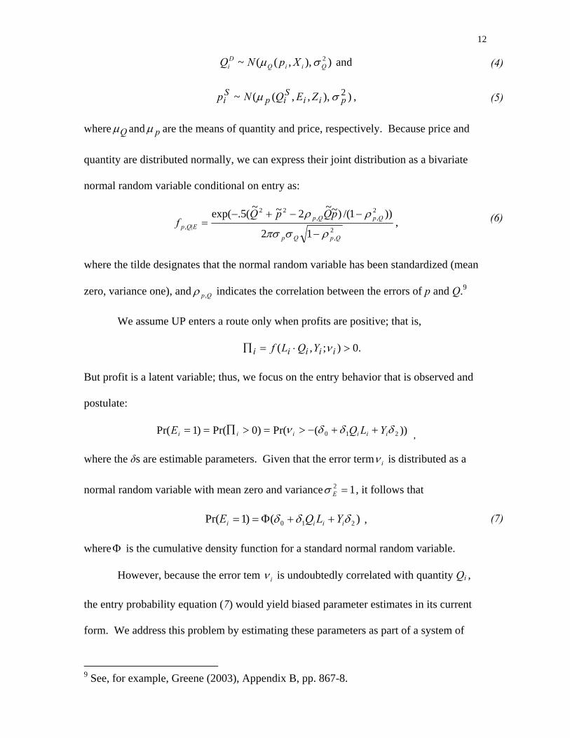
12
)),,((~ 2QiiQ
Di XpNQ σµ and (4)
)),,,((~ 2pii
Sip
Si ZEQNp σµ , (5)
where Qµ and pµ are the means of quantity and price, respectively. Because price and
quantity are distributed normally, we can express their joint distribution as a bivariate
normal random variable conditional on entry as:
2,
2,,
22
|,12
))1/()~~2~~(5.exp(
QpQp
QpQpEQp
pQpQf
ρσπσ
ρρ
−
−−+−= , (6)
where the tilde designates that the normal random variable has been standardized (mean
zero, variance one), and Qp ,ρ indicates the correlation between the errors of p and Q.9
We assume UP enters a route only when profits are positive; that is,
.0);,( >⋅=∏ iiiii YQLf ν
But profit is a latent variable; thus, we focus on the entry behavior that is observed and
postulate:
))(Pr()0Pr()1Pr( 210 δδδν iiiiii YLQE ++−>=>∏== ,
where the δs are estimable parameters. Given that the error term iν is distributed as a
normal random variable with mean zero and variance , it follows that 12 =Eσ
(7) )()1Pr( 210 δδδ iiii YLQE ++Φ== ,
whereΦ is the cumulative density function for a standard normal random variable.
However, because the error tem iν is undoubtedly correlated with quantity Qi ,
the entry probability equation (7) would yield biased parameter estimates in its current
form. We address this problem by estimating these parameters as part of a system of
9 See, for example, Greene (2003), Appendix B, pp. 867-8.

13
equations where we treat entry, price, and quantity as endogenous and obtain consistent
estimates of their parameters in the appropriate equations using exogenous variables in
the entire system as instruments.
Given that we can obtain a consistent estimate for δ1 accounting for the
correlation between the errors of the entry and demand equation ρE,Q , we can write the
conditional probability density function for entry as a binomial random variable:
[ ] ..))((1)1(
))(()|(
2,10
2,10
δρδδ
δρδδ
iiiQEi
iiiQEiiiE
YLQE
YLQEQEf
+⋅+Φ−−
++⋅+Φ=
(8)
If , only the first term in the equation is “switched on,” and if , only the
second term is.
1=iE 0=iE
We can now derive the joint density of entry, price, and quantity as the product of
the conditional density given in equation (8) and the marginal density of price and
quantity, namely:
QpQpEQpE fff ,,|,, ⋅= . (9)
The marginal density can be written as a weighted sum of bivariate normal random
variables. In equation (6), supply price is conditional on entry. To obtain the
unconditional distribution, we evaluate the price given in equation (5) for entry values of
E=1 and E=0, which yields:
0,1,, )0Pr()1Pr( == ⋅=+⋅== EQpEQpQp fEfEf . 10 (10)
10 When we substitute entry into the stochastic formula for price given in equation (5), we account for ρp,E , the correlation of error terms in the inverse supply equation and in the entry equation.

14
Using equation (9), our joint probability distribution is then equal to the product of
equations (8) and (10), which we denote as . As noted, we are simultaneously
computing the entry probabilities as stochastic functions of instrumented quantity.
QpE ,,f
Θ
Given the joint probability density function, the likelihood function we wish to
maximize with respect to the parameters of the demand (1), supply (2), and entry (3)
models, (including the ρs), is the product taken over all N observations
∏=
Θ=ΘN
iQpEfL
1,, ;)( .
In our estimations, the demand and supply equations take a logarithmic functional form,
which is plausible (see, for example, Porter (1983)) and fits the data better than a linear
functional form.
Sample and Estimation Results
Our empirical analysis is based on the shipping activity of the 48 electric utility
plants in operation from 1984 to 1998 that burned at least one million tons of Powder
River Basin coal in a representative year, 1995. The sample ends at 1998 because by
1999 electric utilities began to win a handful of maximum rate cases before the Surface
Transportation Board, so recent reductions in coal rates could potentially be attributable
to residual regulation.11
The plants in our sample account for nearly 75 percent of all Powder River Basin
coal shipped by rail. Of the 48 plants, 31 were served by a single railroad throughout the
sample period and 17 experienced entry sometime between 1985 and 1998. Of the 17
11 No utilities in our sample received a lower rail rate during 1984-98 by winning a maximum rate proceeding.

15
plants, 10 used only PRB coal. A few of the single-served plants came on line after 1984,
thus our final sample consists of 696 observations.
The data sources for the variables used in our analysis and their sample means are
presented in table 1. It is important to point out that virtually all railroad coal traffic is
transported under private contracts that do not reveal the shipper’s rate. Thus, we
collected publicly available data from the U.S. Department of Energy, Energy
Information Administration, and estimated rail rates for electric utilities as the difference
between the delivered price per ton of coal that is consumed at the plant and the price per
ton of coal at the mine mouth. The delivered price of coal reported by the utility includes
all the costs incurred by the utility in the purchase and delivery of the fuel to the plant
(FERC (1995)). The mine mouth price reported by the mine is the total revenue received
using the actual F.O.B. rail sales price (EIA (1995)). Dividing the difference by the
length of haul yields price per ton-mile. Subsequent discussions that we had with railroad
personnel confirmed that our estimates of rail rates in PRB markets were quite close to
actual rail rates.
Based on these data, a simple comparison of freight rates in monopoly and
duopoly markets from 1995 to 1998 suggests that a second entrant has reduced rates and
that rates in duopoly markets have fallen over time as contracts between the incumbent
carrier and shippers have expired (table 2). Of course, this comparison does not hold
other influences on rates constant; we do so by estimating our model of rail transportation
supply, demand, and entry in Powder River Basin markets.
Full information maximum likelihood (FIML) estimates of the model are
presented in table 3. As noted, we specified a time trend to control for unobserved
temporal effects and fixed utility and plant effects, but they were statistically

16
insignificant in the supply, demand, and entry equations and their exclusion had little
effect on the other parameter estimates so they are not included in the specification
presented here.12 Generally, the coefficients have their expected signs and are
statistically significant. The demand for rail transportation of coal is inelastic, which is
plausible. The demand elasticity of –0.38 is aligned with previous research and reflects
the small share of transport costs in the price of electricity and consumers’ inelastic
demand for electricity.13 Another factor that may limit plants’ response to coal rates is
that utilities tend to run their larger coal-fired plants at close to operational capacity—
which in most cases is fixed for the period covered by our sample. Given that the
marginal revenue associated with an inelastic industry demand curve is negative, it
appears that railroads are not engaging in single-period collusive profit maximization or
Cournot behavior. However, this conclusion may be premature to the extent that the
carriers’ conduct is consistent with either form of behavior subject to constraints imposed
by competition in wholesale electricity markets or the threat of maximum rate
regulation.14
The elasticity of rail prices with respect to tons shipped in the inverse supply
equation, 0.02, is not statistically significantly different from zero, indicating that rail is
operating at constant returns to scale. Although railroads generally exhibit economies of
traffic density (Braeutigam (1999)), our finding indicates that they are able to exhaust
12 We also interacted the fixed effects with operating costs to allow this variable to vary across plants, but the fixed effects were statistically insignificant. 13 Winston, Grimm, Corsi, and Evans’ (1990) estimate of the price elasticity of demand for rail transportation of coal was –0.33. 14 It should also be noted that we have estimated the market, as opposed to individual firms’, demand curve. Given the zero-sum nature of competition in the transportationmarket, UP gains traffic at the expense of BN, a firm may enter a market only if it can operate on the elastic part of its demand curve.

17
these economies in PRB markets by moving large shipments in unit coal trains. Bitzan
and Keeler (2003) also find that railroads exhaust economies of density at some point.
The parameter estimates for the rail competition variables in the (inverse) supply
equation are of central importance for our purposes. We find that the initial entry of a
second carrier into a Powder River Basin market reduces rail rates 15 percent and that
this effect becomes stronger over time, albeit at a diminishing rate.15 For example, after
four years of entry, during which time some contracts are likely to have expired, a second
entrant will have reduced rail rates by a third.16 As stressed throughout the paper, coal
shippers negotiate contract rates with railroads that generally last for several years.
According to our findings, contract rates dampen the initial impact that a new rail entrant
has on observed prices. But as shippers’ contacts expire they are able to play one
railroad off against another and obtain lower rates when they negotiate new contracts.
Apparently, carriers have not been successful in reaching a tacit understanding to prevent
such competition from developing.17 As noted, we did not expect potential competition
to have an influence on rate rates. If it did, its effect would be partly captured in the time
15 We also estimated a model that lagged the initial entry variable, but this did not lead to a better statistical fit. 16 Based on our coefficients, this estimate is obtained by calculating: (1-exp(-0.161))+ln(1+ 4 years)*0.117=33.7 percent. We expressed the persistent effect of rail entry as ln(1 + years of entry) because ln(1) =0 and ln (0) is undefined. This specification captures diminishing marginal reductions in rail prices caused by the entry of a second carrier. We explored other functional forms for this variable including a Box-Cox transformation and also specified time dummies to indicate specific years since the entry of the second carrier, but this functional specification produced the best statistical fit. 17 Scherer (1990) provides examples in other industries where large buyers play one seller off against another to elicit price concessions.

18
trend or year dummies as UP entered more markets, but these variables were statistically
insignificant.
The remaining parameter estimates reflect the workings of standard economic
forces. Rail prices respond to operating costs, economies of distance, and other sources
of competition.18 A 1 percent rise in rail operating costs increases rail rates roughly 2
percent. This finding is consistent with the railroad industry’s residual regulatory
environment that allows carriers to set rates that are 180 percent above variable costs
(Dennis (2001)). In addition, many markets in our sample are served by only one carrier.
A 1 percent increase in the length of haul decreases rates 0.17 percent. Similar
economies of distance have been found in other studies (Braeutigam (1999)). Rail source
competition lowers rail rates almost 20 percent, while water source competition lowers
rail rates 14 percent. However, each of these forms of competition has less impact on
prices than a second entrant in the Powder River Basin has after just one year.19 This
finding is consistent with Grimm and Winston’s (2000) estimate of the relative impact of
direct and source competition on rail rates.
Utilities demand more coal shipped by rail from the Powder River Basin as their
nameplate capacity increases, as natural gas prices rise, and after the passage of the Clean
Air Act of 1990. We also find that electric utilities located in the South have a greater
demand than other utilities in the country for coal shipped by rail from the Powder River
18 It has been argued that shippers who provide their own rail cars reduce rail costs and thus receive a lower rate. We specified the percentage of a utility’s coal traffic that is shipped in its private cars in the inverse supply equation, but it had a statistically insignificant effect on rail prices and is not included here. We suspect that this finding is due to the fact that most of the plants in our sample ship large shares of their coal in private cars. 19 After one year, a second entrant in the PRB reduces rail prices by (1-exp(-0.161)) + ln(1+1 year)*0.117=23 percent.
19
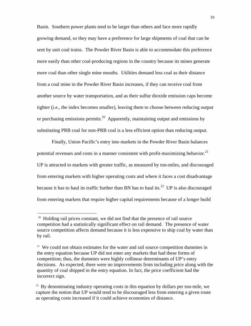
Basin. Southern power plants tend to be larger than others and face more rapidly
growing demand, so they may have a preference for large shipments of coal that can be
sent by unit coal trains. The Powder River Basin is able to accommodate this preference
more easily than other coal-producing regions in the country because its mines generate
more coal than other single mine mouths. Utilities demand less coal as their distance
from a coal mine in the Powder River Basin increases, if they can receive coal from
another source by water transportation, and as their sulfur dioxide emission caps become
tighter (i.e., the index becomes smaller), leaving them to choose between reducing output
or purchasing emissions permits.20 Apparently, maintaining output and emissions by
substituting PRB coal for non-PRB coal is a less efficient option than reducing output.
Finally, Union Pacific’s entry into markets in the Powder River Basin balances
potential revenues and costs in a manner consistent with profit-maximizing behavior.21
UP is attracted to markets with greater traffic, as measured by ton-miles, and discouraged
from entering markets with higher operating costs and where it faces a cost disadvantage
because it has to haul its traffic further than BN has to haul its.22 UP is also discouraged
from entering markets that require higher capital requirements because of a longer build
20 Holding rail prices constant, we did not find that the presence of rail source competition had a statistically significant effect on rail demand. The presence of water source competition affects demand because it is less expensive to ship coal by water than by rail. 21 We could not obtain estimates for the water and rail source competition dummies in the entry equation because UP did not enter any markets that had these forms of competition; thus, the dummies were highly collinear determinants of UP’s entry decisions. As expected, there were no improvements from including price along with the quantity of coal shipped in the entry equation. In fact, the price coefficient had the incorrect sign.
22 By denominating industry operating costs in this equation by dollars per ton-mile, we capture the notion that UP would tend to be discouraged less from entering a given route as operating costs increased if it could achieve economies of distance.
20
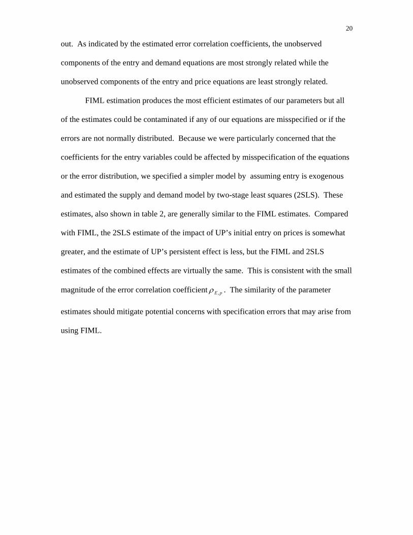
out. As indicated by the estimated error correlation coefficients, the unobserved
components of the entry and demand equations are most strongly related while the
unobserved components of the entry and price equations are least strongly related.
FIML estimation produces the most efficient estimates of our parameters but all
of the estimates could be contaminated if any of our equations are misspecified or if the
errors are not normally distributed. Because we were particularly concerned that the
coefficients for the entry variables could be affected by misspecification of the equations
or the error distribution, we specified a simpler model by assuming entry is exogenous
and estimated the supply and demand model by two-stage least squares (2SLS). These
estimates, also shown in table 2, are generally similar to the FIML estimates. Compared
with FIML, the 2SLS estimate of the impact of UP’s initial entry on prices is somewhat
greater, and the estimate of UP’s persistent effect is less, but the FIML and 2SLS
estimates of the combined effects are virtually the same. This is consistent with the small
magnitude of the error correlation coefficient pE ,ρ . The similarity of the parameter
estimates should mitigate potential concerns with specification errors that may arise from
using FIML.

21
Characterizing Duopoly Behavior
We have argued that rail competition in the Powder River Basin provides a
natural setting for testing theories of duopoly behavior because a monopolist railroad in
the region, Burlington Northern, has gradually begun competing with a new entrant,
Union Pacific, to supply a homogeneous service. We use the FIML parameter estimates
to simulate the effect of UP’s entry on rail prices for coal transportation. This exercise is
complicated by the fact that several other variables besides UP’s entry could affect rail
rates. Thus, we hold all variables except UP’s entry variable and its persistent effect on
prices at their 1984 levels—that is, before UP began entering PRB markets. We then use
the inverse supply and demand equations to predict market equilibrium prices in response
to the changes in UP’s entry behavior over time.
We can assess which theory of duopoly behavior is consistent with the evidence
by comparing the simulated price path with an estimate of the long-run marginal cost of
transporting coal by rail. It is reasonable to make this comparison because in PRB
markets rail is characterized by constant returns to scale—which allows marginal cost
pricing to be financially viable. In addition, shippers and carriers enter into rate
negotiations with a view toward the long run because contracts typically last for several
years. If UP and BN engage in collusive profit-maximizing behavior, simulated prices
should remain at their monopoly (pre-UP entry) level. If the carriers engage in Bertrand
competition, simulated prices should approach marginal cost. And if they engage in
Cournot competition, simulated prices should stabilize between these extremes.
To maintain consistency with the predicted price path, we obtain an independent
estimate of the long-run marginal cost of transporting coal by rail that does not reflect
changes in rail markets after 1984 that may have affected costs. The estimated equation

22
for marginal cost is from Winston, Grimm, Corsi, and Evans (1990) and is based on data
generated in the early 1980s.23 We assume that marginal costs are not affected by UP’s
entry, which is reasonable because PRB coal transportation markets are relatively new,
and both carriers have been able to employ the latest technology and most efficient
operations. Thus, marginal costs are held constant in our simulation.
The price path and long-run marginal cost were converted to 1998 dollars using
appropriate indices; the estimate for the marginal cost of transporting coal in 1984 (in
1998 dollars) is roughly 1.9 cents per ton-mile. Using Bitzan and Keeler’s (2003)
railroad cost function yields a marginal cost estimate for unit train output of 1.8 cents per
ton-mile (in 1998 dollars). Our estimate is also consistent with those obtained by
Bereskin (2001) and Ivaldi and McCullough (2001) that are based on unit train
operations. To repeat, the price path and marginal costs do not represent predictions of
actual rail prices and costs following UP’s entry because other influences on rates and
costs are held constant at their 1984 values.
Figure 2 shows that in the markets that UP has entered at some point between
1984 and 1998, duopoly railroad pricing behavior has evolved slowly, but it can be
reasonably characterized by Bertrand competition because rail prices approach marginal
cost. From 1985 to 1994, rail prices did not change much from their monopoly level.
But since 1994, they have fallen sharply as UP has expanded service to a sufficiently
23 The actual equation for marginal cost is: MC = -$19.06*Route Density + $8.338*Tons + $0.0164*Ton-miles, where route density is ton-miles/route miles; based on the size of the carriers’ networks, we assumed route miles were equal to 20,000. We use this equation to predict the marginal cost of shipping the amount of coal actually transported in each market where UP competes with BN. Because the parameter estimates were obtained using a sample of all commodities shipped by rail and given that we are interested in the marginal cost of transporting coal, the resulting estimate was adjusted by the ratio of the relatively lower cost of shipping bulk versus manufactured commoditiesusing cost estimates in Friedlaender and Spady (1981) and by the relative increase in bulk traffic since deregulation in 1980.

23
large cohort of plants and as BN has been forced to compete with UP for shippers’ traffic
because its contracts have expired.
Although our estimate of long-run marginal cost is consistent with other estimates
in the literature, one could argue that if we (and others) have overestimated marginal
costs by a modest amount, then rail competition would be better characterized by
Cournot than by Bertrand. Recall, however, that Cournot behavior is inconsistent with
our inelastic demand estimate unless railroads are constrained by the threat of maximum
rate regulation—a view that is strongly disputed by captive shippers. Moreover, we
estimate that roughly half of the 54 percent decline in actual rail prices from 1984 to1998
could be attributed to the additional competition supplied by UP and, as shown in table 2,
prices were still declining in duopoly markets in the final years of our sample. As time
continues to pass following the entry of a second carrier and as contracts continue to
expire after 1998, the price path would undoubtedly draw closer to marginal cost even if
the latter were somewhat lower than we estimated.
Indeed, the pervasive use of contract rates in rail freight transportation is probably
the most important reason why Bertrand’s prediction is realized. Each carrier faces the
prospect of getting none of a utility’s business for several years unless it lowers its rate in
response to a competitor’s bid. Given that a typical contract might call for five million
tons of coal to be shipped annually for at least five years, a railroad has a lot to lose if it
does not compete fiercely for a utility’s business and allows the utility to take its traffic
elsewhere.
Another factor that facilitates Bertrand competition is that coal transportation is a
homogeneous commodity. Both BN and UP use the same technology to transport coal

24
from the same source over similar routes, often using cars that are supplied by the
shippers themselves. The average of and variability in their transit times are similar, and
the low value of coal ensures that shippers place little weight on non-transport logistics
costs. All these factors make it extremely difficult for either railroad to convince
shippers that they are providing a different, let alone superior, service. Product
differentiation, primarily through advertising, can explain why some oligopolists have
been able to maintain high price-cost margins (e.g., Baker and Bresnahan (1985)). This
strategy, however, is not effective in rail freight transportation.
Finally, given that BN initially provided rail service for all the utilities that
demanded PRB coal, UP did not have any profits to lose by supplying additional capacity
in this market. Moreover, UP could gain revenue from additional traffic only by cutting
into BN’s traffic. Thus, the two were likely to end up as Bertrand competitors because it
is more difficult to behave as Cournot competitors in zero-sum situations.
Conclusions
We have developed a model of railroad transportation markets for coal to test one
of the oldest controversies in economic theory: How are prices determined in duopoly
markets? Of the available theories, we have found that rail competition in the Powder
River Basin is most accurately characterized by Bertrand’s theory that price-setting
duopolists will sell their identical product at the competitive price.
This finding is of broad interest because recent theoretical work related to
duopoly behavior has included game theoretic models that focus on outcomes between
the polar cases of profit-maximizing collusion and marginal cost pricing. Perfectly
25
competitive outcomes are generally thought to be a rarity. Our results suggest that more
theoretical attention should be given to the factors that generate Bertrand competition.
Empirical evidence of Bertrand competition is also of interest to policymakers as
they ponder whether there is sufficient competition in the railroad industry. Grimm and
Winston (2000) addressed shippers’ and carriers’ dissatisfaction with the Surface
Transportation Board by recommending that policymakers encourage these parties to
negotiate an end to the Board, which would allow full deregulation to go forward. As
part of the negotiations, shippers and carriers would agree on conditions that would
enable captive shippers to have access to another rail carrier. The evidence obtained here
indicates that that the direct competition resulting between two rail carriers is sufficient
to generate low rates for shippers.24
In addition to railroads, policy issues surrounding duopoly competition have
arisen in industries such as telecommunications and electricity as they slowly undergo the
transition to partial deregulation. This paper has identified some of the competitive
conditions that are conducive to Bertrand competition. Future work may be able to build
on this evidence to identify other duopoly markets that are likely to be characterized by
this type of behavior.
24 Negotiations would also recognize that although railroads’ profitability has improved since deregulation, the industry is not yet earning a normal rate of return.

26
Baker, Jonathan B. and Timothy F. Bresnahan, “The Gains from Merger or Collusion in Product-Differentiated Industries,” Journal of Industrial Economics, 33, June 1985, pp. 427-444. Bereskin, C. Gregory, “Sequential Estimation of Railroad Costs for Specific Traffic,” Transportation Journal, 40, Spring 2001, pp. 33-45. Bitzan, John D. and Theodore E. Keeler, “Productivity Growth and Some of Its Determinants in the Deregulated U.S. Railroad Industry,” Southern Economic Journal, 70, October 2003, pp. 232-253. Braeutigam, Ronald R. ,”Learning About Transport Costs,” in Jose Gomez-Ibanez, William B. Tye, and Clifford Winston, editors, Essays in Transportation Economics and Policy: A Handbook in Honor of John R. Meyer, Brookings Institution, Washington DC, 1999. Brander, James A. and Anming Zhang, “Market Conduct in the Airline Industry: An Empirical Investigation,” RAND Journal of Economics, 21, Winter 1990, pp. 567-583. Brander, James A. and Anming Zhang, “Dynamic Oligopoly Behavior in the Airline Industry,” International Journal of Industrial Organization, 11, September 1993, pp. 407-435. Berry, Steven T., “Estimation of a Model of Entry in the Airline Industry,” Econometrica, 60, July 1992, pp. 889-917. Bresnahan, Timothy F. and Peter C. Reiss, “Entry in Monopoly Markets,” Review of Economic Studies, 57, October 1990, pp. 531-553. Bresnahan, Timothy F. and Peter C. Reiss, “Entry and Competition in Concentrated Markets,” Journal of Political Economy, 99, October 1991, pp. 977-1009. Dennis, Scott M., “Changes in Railroad Rates Since the Staggers Act,” Transportation Research Part E: Logistics and Transportation Review, 37, March 2001,
pp. 55-69. Federal Energy Regulatory Commission (FERC), Form 423, Monthly Report of Cost and Quality of Fuels for Electric Plants, 1995. Fischer, Thorsten and David R. Kamerschen, “Price-Cost Margins in the U.S. Airline Industry Using a Conjectural Variation Approach,” Journal of Transport Economics and Policy, 37, May 2003, pp. 227-259.
References

27
Friedlaender, Ann and Richard Spady, Freight Transport Regulation, MIT Press, Cambridge, Massachusetts, 1981. Greene, Willaim, H., Econometric Analysis 5th edition, Prentice Hall, New Jersey, 2003. Grimm, Curtis and Clifford Winston, “Competition in the Deregulated Railroad Industry: Sources, Effects, and Policy Issues,” in Sam Peltzman and Clifford Winston, editors, Deregulation of Network Industries: What’s Next?, Brookings Institution, Washington, DC, 2000. Grimm, Curtis, Clifford Winston, and Carol Evans, “Foreclosure of Railroad Markets: A Test of Chicago Leverage Theory,” Journal of Law and Economics, 35, October 1992, pp. 295-310. Ivaldi, Marc and Gerard McCullough, “Density and Integration Effects on Class I U.S. Freight Railroads,” Journal of Regulatory Economics, 19, March 2001, pp. 161-182. Parker, Philip M. and Lars-Hendrik Roller, “Collusive Conduct in Duopolies: Multimarket Contact and Cross-Ownership in the Mobile Telephone Industry,” RAND Journal of Economics, 28, Summer 1997, pp. 304-322. Porter, Robert H., “A Study of Cartel Stability: The Joint Executive Committee, 1880- 1886,” Bell Journal of Economics, 14, Autumn 1983, pp. 301-314. Scherer, F.M., Industrial Market Structure and Economic Performance, 2nd edition, Rand McNally, Chicago, 1990. Schmalensee, Richard, Paul L. Joskow, A. Denny Ellerman, Juan Pablo Montero, and Elizabeth M. Bailey, “An Interim Evaluation of Sulfur Dioxide Emissions Trading,” Journal of Economic Perspectives, 12, Summer 1998, pp. 53-68. Schmidt, Stephen, “Market Structure and Market Outcomes in Deregulated Rail Freight Markets,” International Journal of Industrial Organization, 19, January 2001, pp. 99-131. United States, Department of Energy, Energy Information Administration (EIA), Form EIA-7A, Coal Production Report. Winston, Clifford, “U.S. Industry Adjustment to Economic Deregulation,” Journal of Economic Perspectives, 12, Summer 1998, pp. 89-110. Winston, Clifford, Thomas Corsi, Curtis Grimm, and Carol Evans, The Economic Effects of Surface Freight Deregulation, Brookings Institution, Washington DC, 1990.

Table 1. Sample Means and Data Sources of the Variables*
Variable Units Mean Data Source Freight charge $/ton-mile 0.017 Energy Information
Administration, Cost and Quality of Fuels and Coal Industry, Annual
Tons of coal shipped 1000 tons 2757 EIA, Cost and Quality of Fuels, Annual
Presence of second rail competitor
Dummy 0.068 Fieldston, Coal Transportation Manual, Annual
Rail source competition
Dummy 0.057 Fieldston, Coal Transportation Manual, Annual
Water source competition
Dummy 0.095 Fieldston, Coal Transportation Manual, Annual
Nameplate Capacity Million KWH
1.172 EIA, Annual Electric Generator Report, form EIA-860, Annual
SO2 emissions caps 1000 tons 2.110 EPA, Clean Air Act, Title IV
Natural gas price $/1000ft3 2.449 EIA, Historical Gas Annual, 2000
Rail industry operating expenses
$ Billions 30.60 American Association of Railroads, Railroad Facts, Annual
Length of haul from mine to plant
Miles 1024 RDI, Coal Rate Database, 1997
Length of “Build-Out” for entrant in 1984
Miles 9.204 Rand McNally, Railroad Atlas (1982) and Commercial Atlas and Marketing Guide (1991)
Incumbent length of haul minus new entrant length of haul
Miles 34.92 Rand McNally, Railroad Atlas (1982) and Commercial Atlas and Marketing Guide (1991)
*All values are in 1998 dollars where appropriate.

Table 2. Comparison of Rail Rates in Monopoly and Duopoly Markets*
Year Average Freight Charge: Monopoly Markets
Average Freight Charge: Duopoly Markets
1995 1.36 1.24
1996
1.29 1.11
1997 1.32 1.08
1998 1.28 1.06
*All freight charges are in 1998 cents per ton-mile

Table 3. Structural Supply, Demand, and Entry Parameter Estimates (Standard Errors are in parentheses) * denotes that the variable has been transformed by natural logarithm.
FIML Coefficients 2SLS Coefficients Variable Supply Demand Entry Supply Demand Freight charge ($/ton mile)* Dependent
Variable -0.382 (0.150)
-- Dependent Variable
-0.812 (0.237)
Tons of coal shipped to plant (thousands)* 0.019 (0.023)
Dependent Variable
0.122 c
(0.056) 0.071
(0.023) Dependent Variable
Supply Characteristics Direct rail competition dummy (1 if a plant can __receive Powder River Basin coal from two __competing railroads; 0 otherwise)
-0.161 (0.051)
-- Dependent Variable
-0.186 (0.076)
--
Number of years after the onset of competition that a __second rail competitor offers a plant service from __the Powder River Basin; (1 + years of entry)*
-0.117 (0.030)
-- -- -0.085 (0.040)
--
Rail industry operating expenses a* 2.032 (0.105)
-- -2.032 (0.408)
2.157 (0.114)
--
Demand Characteristics Plant Nameplate Capacity (millions of KWH) -- 0.626
(0.049) -- -- 0.631
(0.054) Average national price of natural gas ($/1000ft3) -- 0.163
(0.085) -- -- 0.231
(0.108) Clean Air Act (1990) dummy (1 if the Clean Air Act __has been passed; 0 otherwise)
-- 0.640 (0.142)
-- -- 0.515 (0.164)
South regional dummy (1 if plant is located in the __South; 0 otherwise)b
-- 0.859 (0.098)
-- -- 0.902 (0.127)
Plant SO2 emissions cap index (defined as 1 – (emissions cap)-1 for plants subject to emissions caps; 1 for plants not subject to caps)
-- 0.319 (0.149)
-- -- 0.360 (0.143)
Shipment Characteristics Length of haul from mine mouth to plant (miles)* -0.173
(0.028) -0.602 (0.097)
0.122c
(0.056) -0.178 (0.034)
-0.693 (0.129)
Difference in potential entrant’s and incumbent’s __length of haul (miles)
-- -- -0.006 (0.001)
-- --
Build-out distance circa 1984 (miles)*
-- -- -0.296 (0.062)
-- --
Source Competition Rail source competition dummy (1 if a plant can __receive coal from a non Powder River Basin __source by a competing railroad; 0 otherwise)
-0.218 (0.055)
-- -- -0.215 (0.110)
--
Water source competition dummy (1 if a plant can __receive coal from a non Powder River Basin __source by water transportation; 0 otherwise)
-0.156 (0.054)
-1.218 (0.306)
-- -0.078 (0.062)
-1.322 (0.292)
Constant -10.03 (0.467)
8.042 (0.775)
3.874 (1.501)
-10.82 (0.541)
6.777 (1.009)
Other Parameters =Qp,ρ
-0.125 ; (0.020)
=pE,ρ
0.011 ; (0.027)
=QE,ρ
-0.158 (0.123)
=2pσ
0.101 ; (0.006)
=2Qσ
1.208 (0.156)
Summary Statistics Number of Observations 696 696 696 696 696 Log likelihood at convergence -1373.02 -1373.02 -1373.02 -- -- R2 -- -- -- 0.42 0.32

Table 3. Explanatory Notes a Operating expenses are denominated in dollars for supply, and dollars/ton mile for entry. b The South region includes Alabama, Arkansas, Louisiana , Mississippi, Oklahoma, and Texas. c Entry is assumed to be a function of ln(ton miles). Estimation can be facilitated by noting that βln(ton miles) = βln(tons)+ βln(length of haul); that is, tons can be treated as endogenous in this specification if we constrain tons and length of haul to have the same coefficients in the entry equation estimation. We could not statistically reject this specification.

Figure 1. Share of coal used in the United States by origin
Source: EIA Coal Industry Annual, 1994-2000
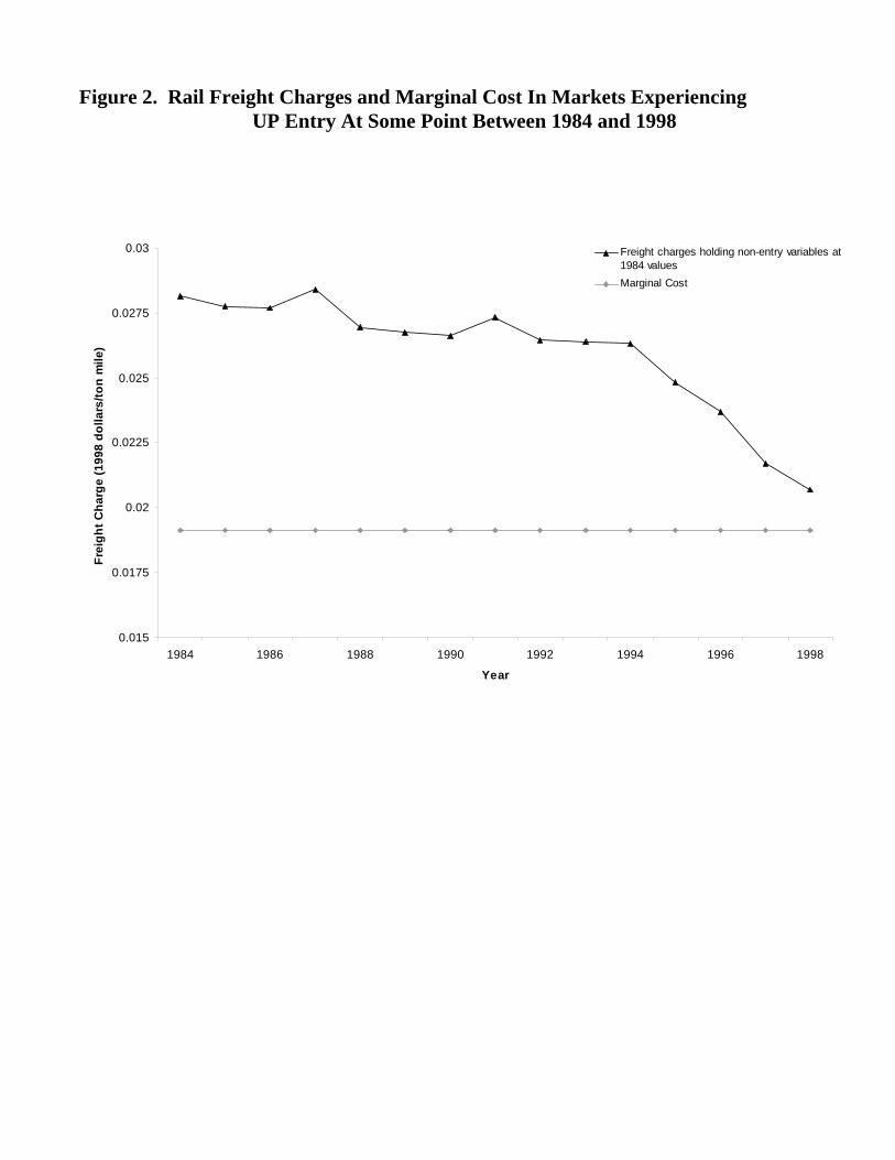
Figure 2. Rail Freight Charges and Marginal Cost In Markets Experiencing UP Entry At Some Point Between 1984 and 1998
0.015
0.0175
0.02
0.0225
0.025
0.0275
0.03
1984 1986 1988 1990 1992 1994 1996 1998
Year
Frei
ght C
harg
e (1
998
dolla
rs/to
n m
ile)
Freight charges holding non-entry variables at1984 valuesMarginal Cost