Policy Research Working Paper 7105

Durable Goods and Poverty MeasurementNicola AmendolaGiovanni Vecchi

Poverty Global Practice GroupNovember 2014

WPS7105P

ublic

Dis

clos

ure

Aut

horiz

edP

ublic

Dis

clos

ure

Aut

horiz

edP

ublic

Dis

clos

ure

Aut

horiz

edP

ublic

Dis

clos

ure

Aut

horiz

edP

ublic

Dis

clos

ure

Aut

horiz

edP

ublic

Dis

clos

ure

Aut

horiz

edP

ublic

Dis

clos

ure

Aut

horiz

edP

ublic

Dis

clos

ure

Aut

horiz

ed

Produced by the Research Support Team

Abstract

The Policy Research Working Paper Series disseminates the findings of work in progress to encourage the exchange of ideas about development issues. An objective of the series is to get the findings out quickly, even if the presentations are less than fully polished. The papers carry the names of the authors and should be cited accordingly. The findings, interpretations, and conclusions expressed in this paper are entirely those of the authors. They do not necessarily represent the views of the International Bank for Reconstruction and Development/World Bank and its affiliated organizations, or those of the Executive Directors of the World Bank or the governments they represent.

Policy Research Working Paper 7105

This paper is a product of the Poverty Global Practice Group. It is part of a larger effort by the World Bank to provide open access to its research and make a contribution to development policy discussions around the world. Policy Research Working Papers are also posted on the Web at http://econ.worldbank.org. The authors may be contacted at giovanni.vecchi@uniroma2.it.

The paper focuses on durable goods and their role in the measurement of living standards. The paper reviews the theoretical underpinnings of the methods available to estimate the value of the services flowing from consumer durable goods. It also provides a unified framework that

encompasses the acquisition approach, the rental equiv-alent approach, and the user cost approach. The pros and cons of each method are discussed in the context of poverty and inequality analysis and it is argued that the user cost should receive the highest consideration.

Durable Goods and Poverty Measurement

Nicola Amendola1 and Giovanni Vecchi23

JEL: C46, D31, I32, O15

Keywords: Measurement of poverty; Inequality; Consumption aggregate, Income Distribution

1 University of Rome “Tor Vergata” 2 University of Rome “Tor Vergata” 3 We are grateful to Lidia Ceriani, Sergio Olivieri, Marco Ranzani, Carlos Felipe Balcazar and Nobuo Yoshida for the useful comments

received.

1 Introduction

When it comes to measuring inequality and poverty, the choice and definition of an

appropriate welfare indicator is not a straightforward task. A number of decisions must be

made, many of which are controversial, and most often the decision making process is

based on well-established practices rather than on theoretical arguments (Lanjouw, 2009;

Deaton and Zaidi 2002). In this paper we focus on consumer durable goods and investigate

their contribution to determining the living standard of the household.

In general, long-lived items such as automobiles, appliances and furniture have a positive

and significant impact on living standards. Sometimes the outlay on durable goods only

claims a small fraction of disposable income, but they most often change the lifestyle of the

individuals, either by saving their time – as in the case of housework appliances – or by

consuming their time, as with entertainment appliances (Offer 2005). Either way, consumer

durable goods clearly matter to the wellbeing of individuals and there is an increasing

consensus on the fact that any welfare measure should account for them (Slesnik, 2001,

Deaton and Zaidi 2002, OECD 2013).

In the first part of this paper we review the theoretical underpinnings of the methods

available to deal with durables. We outline the main alternatives found in the literature and

discuss their advantages and disadvantages in the context of poverty and inequality

analysis. We end up our review by arguing that the so-called “user cost approach” is well

worth our recommendation (Diewert 2009). The underlying idea is that it is not the

expenditures on consumer durables that should be included in the welfare aggregate. Rather,

it is the flow of services from durables that must be valued and comprised in the welfare

aggregate, and the user cost method estimates it simply by calculating the difference

between the value of the durable at the beginning of analytical the period and its actual

value at the end of the same period. While simple, this method is not naïve, and offers the

2

further advantage (not shared by the rental equivalence approach) of being a viable solution

given the information typically available in household budget surveys.

The second part of the paper is devoted to measurement issues. What is simple in theory

can turn into a thorny problem in practice. In fact, the estimation of the user cost of durable

goods is an exercise fraught with difficulties. Data limitation is probably the single most

important obstacle to implementing the user cost method. We discuss how data limitations

can be overcome, or at least dealt with, by overviewing the current practice for a number of

countries all around the world.

PART I – THEORY

2 Concepts and definitions

What is a durable good and why durable goods require a special treatment? These are two

focal questions that need to be addressed before outlining the theoretical approaches

available to deal with consumer durable goods and their role in the measurement of living

standards.

A durable good is a consumption good that can “deliver useful services to a consumer

through repeated use over an extended period of time” (Diewert, 2009 p. 447). The main

characteristic of a durable good does not depend on its physical durability, a property

shared by many other consumption goods, but by the fact that, like capital goods, it is

productive for two or more periods. According to the System of National Accounts (SNA)

– the internationally agreed set of recommendations on how to compile measures of

economic activity – “….the distinction is based on whether the goods can be used once

only for purposes of production or consumption or whether they can be used repeatedly, or

continuously. For example, coal is a highly durable good in a physical sense, but it can be

burnt only once. A durable good is one that may be used repeatedly or continuously over a 3

period of more than a year, assuming a normal or average rate of physical usage. A

consumer durable is a good that may be used for purposes of consumption repeatedly or

continuously over a period of a year or more.” (SNA 2008: 184). Housing is clearly a

durable good, arguably among the most important ones in most consumers’ bundles. Due to

its importance, however, the way rents and imputed rents are estimated for inclusion in the

welfare aggregate is the object of a separate paper.4 In this paper we focus on consumer

durable goods other than housing5.

The SNA definition helps to answer the second question, namely why durable goods

require special treatment when measuring living standards. The essence of the problem lies

in the inconsistency between the so-called reference period chosen for the welfare

aggregate, and the period of time during which durable goods deliver their utility to the

consumer. In theory, prior to the analysis, “we need to decide the reference period for

welfare measurement, whether someone is poor if they go without adequate consumption or

income for a week, a month, or a year” (Deaton 1997: 151). Once this choice is made, the

same reference period must be applied to all the components of the welfare aggregate, no

matter if it is pears or t-shirts, electric fans or cars. In practice, very rarely the reference

period exceeds one year; most often, it coincides with the year6. If we assume that the

reference period is one year (or less), then it is clear that durable goods, by their very

4 This follows a well-established practice according to which, a welfare aggregate is constructed by putting

together four building blocks, namely (i) food consumption, (ii) non-food consumption, (iii) durable goods

and (iv) housing [Deaton and Zaidi 2002: 25]. 5 According to the Classification of individual consumption by purpose (COICOP) nomenclature,

consumption goods are classified as non durable (ND), semi-durables (SD) and durable (D). The consumption

goods classified as durable belong to the following categories: furniture, furnishings, carpets and other floor

coverings, major household appliances, tools and equipment for house and garden, therapeutic appliances and

equipment, vehicles, telephone and fax equipment, audiovisual, photographic and information processing

equipment (except recording media), major durables for recreation, electrical appliances for personal care,

jewelry, clocks and watches (ILO, 2004). 6 In most LSMS questionnaires the recall period for nonfood items does not exceed one year.

4

definition, pose a problem: how to reconcile the fact that items whose economic life

extends beyond the reference period of the welfare aggregate must be part of it?

The purchasing market price of a durable good is clearly an inadequate pricing concept.

This is because the purchasing market price corresponds to the value of the durable good

for its entire economic life, while what we need is the value of the use of durable goods for

a shorter period, the reference period. Unfortunately, the value of the use of a durable that

contributes to the welfare during the reference period is rarely, if ever, directly observed.

This explains why durable goods require special treatment: the expression coined in the

literature is that we need to estimate the consumption flow of durable goods, that is to

estimate the benefit accruing to the household from the ownerships of durable goods,

limited to the reference period of analysis.

The impact of using the consumption flow instead of the purchasing price of the durable

depends on the purposes of the analysis. Let us start with the context of the system of

national accounts (Moulton 2004; Young 2005). The value of expenditures on consumer

durables tend to fluctuate widely over the business cycle, while the value of their services

(the consumption flow) varies more smoothly. This suggests that the latter measure

provides a better picture than the former of the changes of a nation’s economic welfare over

time and make international comparisons more meaningful Katz (1983: 406). While the

2008 SNA recognizes these advantages, in practice, “the SNA measures household

consumption by expenditures and acquisitions only. The repeated use of durables by

households could be recognized only by extending the production boundary by postulating

that the durables are gradually used up in hypothetical production processes whose outputs

consist of services. These services could then be recorded as being acquired by households

over a succession of time periods. However, durables are not treated in this way in the

SNA. A possible supplementary extension to the SNA to allow for such an extension of the

production boundary could usefully take place in a satellite account.” (SNA 2008: 184).

A similar issue arises in the construction of a consumer price index (CPI). As argued by

Alchian and Klein (1973), any analytically correct measures of inflation should take

account of changes in the price of durable goods. The point was, in fact, made by Irving

5

Fisher as far back as 1911, when he explained that to base a price index only on “services

and immediately consumable goods would be illogical” (Fisher 1911: ch. 10, X.39). The

claim that durable goods should be covered by the consumer price index has never been

disputed from a theoretical standpoint. Yet, in practice, the task of incorporating the price

dynamics of consumer durables is not straightforward. A special treatment of the prices of

durables is often necessary in order to moderate the observed volatility in measures of

inflation that incorporate changes in the price of assets (Goodhart, 2001). Even more

relevant to the present context is the fact that if the CPI is to serve as a cost-of-living index,

then the pricing concept should hinge on the cost of the use of the services of the durable

good during the reference period rather than on its purchase price (Diewert 2004, 2009).

When it comes to measuring living standards, poverty and inequality, the estimation of the

value of consumer durables is also crucial. The use of the purchase price instead of the

consumption flow leads to overestimate the effect of economic cycle on the household

welfare, to underestimate absolute poverty, and most likely to bias the poverty profile

(Deaton and Zaidi 2002). A well-documented study on Russia, for instance, shows that the

impact on inequality can be very large: the Gini index of expenditure increases from 32

percent to 44 percent when the full purchase value of durables is included instead of its use

value (World Bank 2005: 9).

Irrespective of the angle that one may take, the estimation of the consumption flow from

durable goods stands out as a complex task. The main reason is that the value of the flow of

services of a durable depends on its physical deterioration rate but also on the (unobserved)

expected price of the durable7. This imputation exercise can be interpreted as a special case

of the classical problem of the measurement of capital, one of the oldest and most

contentious areas of economic theory (Hicks 1955; Hulten 1990; Downs 1986).

7 There are circumstances were the estimation of the consumption flow is a simple task. If the consumer

purchases the services of durables – for instance renting a car – then the price that s/he pays does the job as it

represents the consumption flow. Unfortunately, in most cases ownership is not separated from usage and

analysts must deal with the imputation problem.

6

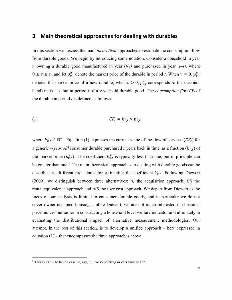
3 Main theoretical approaches for dealing with durables

In this section we discuss the main theoretical approaches to estimate the consumption flow

from durable goods. We begin by introducing some notation. Consider a household in year

t, owning a durable good manufactured in year (t-v) and purchased in year (t–s), where

0 ≤ 𝑠𝑠 ≤ 𝑣𝑣, and let 𝑝𝑝𝑣𝑣,𝑡𝑡𝑠𝑠 denote the market price of the durable in period t, When 𝑣𝑣 = 0, 𝑝𝑝𝑣𝑣,𝑡𝑡

𝑠𝑠

denotes the market price of a new durable; when 𝑣𝑣 > 0, 𝑝𝑝𝑣𝑣,𝑡𝑡𝑠𝑠 corresponds to the (second-

hand) market value in period t of a v-year old durable good. The consumption flow 𝐶𝐶𝐶𝐶𝑡𝑡 of

the durable in period t is defined as follows:

(1) 𝐶𝐶𝐶𝐶𝑡𝑡 = 𝑘𝑘𝑣𝑣,𝑡𝑡𝑠𝑠 × 𝑝𝑝𝑣𝑣,𝑡𝑡

𝑠𝑠

where 𝑘𝑘𝑣𝑣,𝑡𝑡𝑠𝑠 ∈ ℝ+. Equation (1) expresses the current value of the flow of services (𝐶𝐶𝐶𝐶𝑡𝑡) for

a generic v-year old consumer durable purchased s years back in time, as a fraction (𝑘𝑘𝑣𝑣,𝑡𝑡𝑠𝑠 ) of

the market price (𝑝𝑝𝑣𝑣,𝑡𝑡𝑠𝑠 ). The coefficient 𝑘𝑘𝑣𝑣,𝑡𝑡

𝑠𝑠 is typically less than one, but in principle can

be greater than one.8 The main theoretical approaches to dealing with durable goods can be

described as different procedures for estimating the coefficient 𝑘𝑘𝑣𝑣,𝑡𝑡𝑠𝑠 . Following Diewert

(2009), we distinguish between three alternatives: (i) the acquisition approach; (ii) the

rental equivalence approach and (iii) the user cost approach. We depart from Diewert as the

focus of our analysis is limited to consumer durable goods, and in particular we do not

cover owner-occupied housing. Unlike Diewert, we are not much interested in consumer

price indices but rather in constructing a household level welfare indicator and ultimately in

evaluating the distributional impact of alternative measurement methodologies. Our

attempt, in the rest of this section, is to develop a unified approach – here expressed in

equation (1) – that encompasses the three approaches above.

8 This is likely to be the case of, say, a Picasso painting or of a vintage car.

7

3.1 Acquisition approach

When a durable good is purchased by a household and its entire value is attributed to the

household expenditure, we say that the durable good is treated according to the acquisition

approach (also known as “net acquisition approach”). Looking at equation (1), this

approach amounts to specifying the coefficient 𝑘𝑘𝑣𝑣,𝑡𝑡𝑠𝑠 as follows:

(2) 𝑘𝑘𝑣𝑣,𝑡𝑡𝑠𝑠 (𝑎𝑎) = �1 𝑖𝑖𝑖𝑖 𝑠𝑠 = 0

0 𝑖𝑖𝑖𝑖 𝑠𝑠 > 0

In equation (2), the argument “a” in 𝑘𝑘𝑣𝑣,𝑡𝑡𝑠𝑠 (𝑎𝑎) stands for “acquisition”. According to the

acquisition approach, 𝐶𝐶𝐶𝐶𝑡𝑡 = 0 if the household does not purchase the durable during the

survey year t – eq. (2) says that 𝑘𝑘𝑣𝑣,𝑡𝑡𝑠𝑠 (𝑎𝑎) = 0 for all items for which s>0, that is for items

purchased prior to the current period t. Note that the definition does not contemplate v, that

is, it does not matter if the durable is new or used. A positive consumption flow 𝐶𝐶𝐶𝐶𝑡𝑡 = 𝑝𝑝𝑣𝑣,𝑡𝑡0

is attributed to durable goods purchased by the household when s=0, that is during the

survey year. Under the assumption that the market price 𝑝𝑝𝑣𝑣,𝑡𝑡0 captures the current value of

all services provided by the durable over its entire economic life, then the net acquisition

approach assigns the household the entire stream of current and future productive services

of the durable in year t and zero for subsequent years.

The acquisition approach ignores the problem of distributing the initial cost of the durable

over the useful life of the good and allocate the entire charge to the period of purchase [ILO

2003: 419]. Further, the acquisition approach is clearly distortionary: it underestimates the

welfare of households that owns used durable goods with respect to households who

happened to purchase durable goods in the current year. 9 When the net acquisition

approach is used for the construction of the consumption aggregate, both the level and the

9 It is certainly true that this distortionary effect is less important if we are interest in aggregated variables but

we cannot say that it completely vanishes (see section 4).

8

budget shares of durables tend to mirror the business cycle. This is due to the fact that

households tend to postpone the purchase of durables when the economy slows down, and

to increase it when the economy boosts.

3.2 Rental equivalence

If rental or leasing markets for consumer durable goods exist, then the market rental prices

can be used to estimating consumption flows from durable goods. This method is known as

the rental equivalence approach [ILO 2003, Diewert 2009]. Suppose that in period t a

competitive market exists, where households can purchase the services of v-year-old

durable goods. Consumers can rent a car or a refrigerator, for example. Also assume that

households own homogeneous durable goods, that is assume that all goods are of the same

type and quality. Let 𝑅𝑅𝑣𝑣,𝑡𝑡 denote the market rental value of the v-year-old durable good. If

markets are competitive and the economy is in equilibrium, then the market rental value

𝑅𝑅𝑣𝑣,𝑡𝑡 measures the consumption flow from the durable owned by the household.10 Going

back to equation (1), the rental equivalence approach specifies 𝑘𝑘𝑣𝑣,𝑡𝑡𝑠𝑠 (𝑟𝑟) as follows:

(3) 𝑘𝑘𝑣𝑣,𝑡𝑡𝑠𝑠 (𝑟𝑟) =

𝑅𝑅𝑣𝑣,𝑡𝑡 𝑝𝑝𝑣𝑣,𝑡𝑡𝑠𝑠

where 𝑅𝑅𝑣𝑣,𝑡𝑡 𝑝𝑝𝑣𝑣,𝑡𝑡𝑠𝑠⁄ is the rental ratio with respect to the market value of the durable owned by

the household, also known as the capitalization rate. In equation (3), the argument “r” in

𝑘𝑘𝑣𝑣,𝑡𝑡𝑠𝑠 (𝑟𝑟) stands for “rental”. If we substitute (3) in (1) we obtain 𝐶𝐶𝐶𝐶𝑡𝑡 = 𝑅𝑅𝑣𝑣,𝑡𝑡 .

In the rental equivalence approach, a pivotal role is clearly played by the market prices for

the services of durable goods. However, three restrictions must be introduced in order to

make the approach fully consistent: (a) one must assume the existence of a complete set of

10 We also do not consider here taxes and transaction costs. 9

markets for the services of the durables owned by the household; (b) markets must be

competitive and (c) the economy must be in equilibrium. If assumption (a) does not hold

we cannot apply the method and if one of the other two assumptions is violated the market

rental value does not reflect necessarily the household welfare gain from using the durable

in period t.

An additional concern with the rental equivalence approach has an empirical nature. The

estimate of 𝑘𝑘𝑣𝑣,𝑡𝑡𝑠𝑠 (𝑟𝑟) in equation (3) requires the availability of market rental prices in period

t for services of vintage-v durable goods. Even if, according to assumption (a), such a

market exists, this does not necessarily imply that actual transactions are available in the

sample. When markets are thin, 1) it can be very difficult to observe rental prices for all the

durables owned by the households, and 2) prices are likely to suffer from heterogeneity11.

The first condition is well-known and well documented in the literature that deals with the

measurement of the cost of shelter for homeowners (see, among the others, Gillingham

1983). One solution for determining rental price equivalents for consumer durables is to ask

households what they think their durables would rent for. Perception, however, does not

always and necessarily matches with reality. Households might have imperfect information

on current market prices especially with regard to consumption goods purchased or sold

infrequently (or never purchased or sold).

3.3 User cost

The user cost approach is based on a concept first introduced by Keynes (1936, chapter 6,

p. 53) and successively reformulated by Jorgenson (1963). The idea behind the approach is

highly intuitive: the user cost approach calculates the cost of purchasing the durable at the

beginning of the period, using the services of the durable during the period and then netting

11 Note that this should not happen if markets were perfectly competitive. Hence, the empirical relevance of

point 2) may indicate a violation of the perfect competition assumption.

10

off from these costs the benefit that could be obtained by selling the durable at the end of

the period (ILO 2003: 422)12.

Let 𝑝𝑝𝑣𝑣,𝑡𝑡𝑠𝑠 denote the market price of a durable produced in year t-v, but purchased in year t-s.

We assume here that the purchase took place at the beginning of period t. Similarly, let

𝑝𝑝𝑣𝑣+1,𝑡𝑡𝑠𝑠+1 denote the market price of the same durable at the end of period t. This notation

(both indices are now v+1 and s+1) reflects the fact that at the end of the period t both the

vintage of the good (v) and its purchase date have increased by one unit. The user cost

evaluated at the end of period t can be defined as follows:

(4) 𝑈𝑈𝐶𝐶𝑡𝑡 = (1 + 𝑖𝑖𝑡𝑡)𝑝𝑝𝑣𝑣,𝑡𝑡𝑠𝑠 − 𝑝𝑝𝑣𝑣+1,𝑡𝑡

𝑠𝑠+1

where 𝑖𝑖𝑡𝑡 is the nominal interest rate in period t.

The user cost can be interpreted as the opportunity cost of owning for one period the

durable instead of selling the durable at the beginning of period t. Equation (4) can be

manipulated to show that the user cost 𝑈𝑈𝐶𝐶𝑡𝑡 equals the sum of the net return of the durable

(in equilibrium, the net return corresponds to what the consumer would obtain by not

purchasing the asset and investing an equivalent amount of money on a competitive

financial market) plus a possible capital gain:

(5) 𝑈𝑈𝐶𝐶𝑡𝑡 = 𝑖𝑖𝑡𝑡𝑝𝑝𝑣𝑣,𝑡𝑡𝑠𝑠���

𝑟𝑟𝑟𝑟𝑡𝑡𝑟𝑟𝑟𝑟𝑟𝑟𝑠𝑠

+ �𝑝𝑝𝑣𝑣,𝑡𝑡𝑠𝑠 − 𝑝𝑝𝑣𝑣+1,𝑡𝑡

𝑠𝑠+1 ����������𝑐𝑐𝑐𝑐𝑐𝑐𝑐𝑐𝑡𝑡𝑐𝑐𝑐𝑐 𝑔𝑔𝑐𝑐𝑐𝑐𝑟𝑟𝑠𝑠

Equation (5) shows that the user cost depends on the current price of the durable 𝑝𝑝𝑣𝑣,𝑡𝑡𝑠𝑠 , on

the current nominal interest rate 𝑖𝑖𝑡𝑡 , but also on expected capital gains, that is on the

12 Alternatively, the user cost can be derived by equating the price of a durable to the discounted value of the

net benefits that it is expected to generate in the future. See Jorgenson (1963) and OECD (2009).

11

expected price of the durable at the end of period t. Thus, the user cost can be interpreted as

an ex-ante measure of the consumption flow. In equation (5), and in the rest of this section,

however, we do not distinguish between expected and actual prices. This amounts to

assuming that the economy is in equilibrium and that the user cost is at the same time an ex

ante and an ex post measure of the consumption flow.

In equation (5), capital gains (or losses) depend on the economic depreciation of the

durable and on the monetary price dynamics of durable goods. Economic depreciation is an

expression used to describe the loss in monetary value that most capital goods experience

with age [Hulten and Wykoff 1981]. Due to economic depreciation, one unit of the

consumer durable of vintage v at the beginning of period t corresponds to (1 − 𝛿𝛿𝑡𝑡) units of

a durable of vintage v+1 at the beginning of the period t, where 𝛿𝛿𝑡𝑡𝜖𝜖(0,1) is usually referred

to as the net depreciation rate.13 At the same time, the price of one unit of a consumption

durable of age v at the end of period t is equal to (1 + 𝜋𝜋𝑡𝑡)𝑝𝑝𝑣𝑣,𝑡𝑡𝑠𝑠 , where 𝜋𝜋𝑡𝑡 measures the

durable-specific inflation rate in period t. It follows that 𝑝𝑝𝑣𝑣+1,𝑡𝑡𝑠𝑠+1 = (1 − 𝛿𝛿𝑡𝑡)(1 + 𝜋𝜋𝑡𝑡)𝑝𝑝𝑣𝑣,𝑡𝑡

𝑠𝑠 .

Substituting in equation (5) we obtain:

(6) 𝑈𝑈𝐶𝐶𝑡𝑡 = [𝑖𝑖𝑡𝑡 + 1 − (1 − 𝛿𝛿𝑡𝑡)(1 + 𝜋𝜋𝑡𝑡)]𝑝𝑝𝑣𝑣,𝑡𝑡𝑠𝑠

If we assume 𝜋𝜋𝑡𝑡𝛿𝛿𝑡𝑡 ≃ 0, equation (6) simplifies to:

13 Hulten and Wykoff (1995) distinguish between “deterioration” and “depreciation”. The former is a quantity

concept while the latter refers to a financial value. Deaton and Zaidi (2002: 14) prefer to use the concept, and

discuss a model for the “deterioration rate” based on the assumption that “the quantity of the good is subject

to “radioactive decay”, so that if the household starts off the year with the amount St, it will have an amount

(1 − 𝛿𝛿𝑡𝑡)𝑆𝑆𝑡𝑡 to sell back at the end of the year”. This model corresponds to the geometric depreciation model

that we introduce in section 5.4.1. Hulten and Wykoff (1995), however observe that under the depreciation

model the two concepts coincide. See also Koumanakos and Hwang (1988)

12

(7) 𝑈𝑈𝐶𝐶𝑡𝑡 = (𝑟𝑟𝑡𝑡 + 𝛿𝛿𝑡𝑡)𝑝𝑝𝑣𝑣,𝑡𝑡𝑠𝑠

where 𝑟𝑟𝑡𝑡 = 𝑖𝑖𝑡𝑡 − 𝜋𝜋𝑡𝑡 is the Fisherian real interest rate. Equation (7) states that the user cost

can be obtained by applying the sum of the real interest rate and the economic depreciation

rate to the market price of an v-year old consumer durable in period t. Hence, according to

the user cost approach, the coefficient 𝑘𝑘𝑣𝑣,𝑡𝑡𝑠𝑠 (𝑢𝑢) is simply:

(8) 𝑘𝑘𝑣𝑣,𝑡𝑡𝑠𝑠 (𝑢𝑢) = 𝑟𝑟𝑡𝑡 + 𝛿𝛿𝑡𝑡

where the argument “u” in 𝑘𝑘𝑣𝑣,𝑡𝑡𝑠𝑠 (𝑢𝑢) stands for “user cost”. Equation (8) helps clarify the

relationship between the user cost and the rent equivalent approaches. The two approaches

produce the same estimate of the consumption flow if and only if 𝑘𝑘𝑣𝑣,𝑡𝑡𝑠𝑠 (𝑢𝑢) = 𝑘𝑘𝑣𝑣,𝑡𝑡

𝑠𝑠 (𝑟𝑟), i.e. if

and only if:

(9) 𝑅𝑅𝑡𝑡 = [𝑟𝑟𝑡𝑡 + 𝛿𝛿𝑡𝑡]𝑝𝑝𝑣𝑣,𝑡𝑡𝑠𝑠

Equation (9) states that the market rental value of the durable in a single period must be

equal to the real rate of return that can be obtained by selling the durable and investing it on

the capital market net of the depreciation rate of the durable. This is clearly an arbitrage

condition that is only satisfied in equilibrium and in absence of any market friction

[Jorgenson 1963, Deaton and Muellbauer, 1980]14.

14 Garner and Verbrugge (2007) find evidence on the empirical divergence between the two measures.

13

4 Discussion

There are clear conceptual and theoretical differences between the three approaches

reviewed in the previous section. The net acquisition approach is a stock approach, while

the rental equivalence and the user cost approaches are flow approaches. If we interpret the

consumer durable as a capital asset, the net acquisition approach consists in valuing both

the present and future productive services of new “capital” by means of the purchasing

market price of the durable. One advantage of this method is that it treats durable goods

symmetrically with non-durable consumption goods. The approach is also conceptually

simple, easy to communicate and parsimonious in terms of data requirement (Diewert,

2004, 2009): its implementation only requires the market value of the durables purchased

by the household in the survey period. A further advantage is its consistency with the

prescriptions of SNA 2008 (SNA 2008). For all these reasons, most statisticians engaged in

constructing consumer price indices adopt the acquisition approach for all durable goods

(with the exception of housing) [ILO 2003: 419].

There are, however, theoretical drawbacks that cannot be ignored. While the adoption of

the acquisition approach might have a relatively little impact on the SNA, especially if the

economy is on a steady state growth pattern15, the same is not true for micro-level analyses.

By imputing the entire value of the durable to the initial (acquisition) period the analyst

clearly misrepresents the time pattern of the welfare accruing to the household that owns

durable goods. The acquisition approach systematically overestimates the living standards

of households who decide to invest on new consumer durables, and underestimate it for

15 Diewert, (2004, 2002) prove that, in a long run equilibrium, the ratio between the value of the consumption

flow estimated according to the user cost approach and the value estimated following the acquisition approach

is constant and is, in general, larger than one. The ratio approximate the unity in a steady state growth pattern

Jorgenson and Lanfeld (2006) note, however, that the distortion induced by the acquisition approach could

also involve the aggregated level analysis. In a boost phase of the business cycle households tend to postpone

investments on durables and the opposite is true in boom phases. Hence, the acquisition approach emphasizes

the cycle giving a large weight to the more volatile component (sensitive to expectation) of households’

consumption expenditure

14

households who decide to postpone this decision or have taken this decision in the past.

While it is not easy to identify the direction and the magnitude of the bias, poverty and

inequality estimates are certainly biased in the presence of durable goods imputed by means

of the acquisition approach.

The above discussion lead us to prefer the rental equivalence and the user cost approaches

to the acquisition approach, at least in the context of welfare analysis. This is in line with

the conclusions reached by Deaton and Zaidi (2002: 35), Diewert (2004, 2009), and more

recently by the OECD Expert Group on Micro-statistics on Household Income,

Consumption and Wealth (OECD, 2013).

As shown in equation (9), in an equilibrium position, the rental equivalence and the user

cost approach are theoretically consistent. The rental equivalence approach uses the market

evaluation (observed paid rent) as an (ex ante) estimate of the user cost. If expectations are

fulfilled, market rents can be considered as a good approximation of the user cost. There

are however two problems. Firstly, if there is uncertainty, the hypothesis of perfect

foresight may not be a plausible one16. In most situations, the rental equivalence approach

is unlikely to converge to the user cost, due to departures from the theoretical conditions

that must hold in order for equation (9) to hold true. Market rental prices for durables are

often sensitive to expectations and other cyclical factors. Secondly, we should consider

certain data issues. For most v-year old durable goods, the availability of actual market

rental prices is the exception rather then the rule. In most developing countries, markets for

durable services are thin or even non existent and this makes the hypothesis of perfect

foresight discussed sub 1) untenable. As appealing as the solution of asking households a

self-assessment of durable rental prices might seem, the absence of reliable market data

would not allow to test the reliability of the answers.

16 The question has been clearly pointed out, even if in a different context, by Hulten and Wykoff (1995):

“The rental price, on the other hand, is the ex ante cost of acquiring the right to use the capital good for a

stipulated period of time. Under perfect foresight with full utilization the two concepts will tend to converge.

With uncertainty, they may not”

15

A combination of theoretical and data-related arguments leads us to express a preference

for the user cost approach. Further, questionnaires used in many household budget surveys

around the world contain useful information for implementing the user cost approach,

irrespective of the choice of the welfare aggregate (in particular, whether income- or

expenditure based). All in all, the user cost provides the best balance between theoretical

consistency and data requirement to properly account for durable goods in measuring

welfare at the household level.

PART II – PRACTICE

In this section we focus on implementation issues, and in particular on how to estimate the

consumption flow of consumer durable goods according to the user cost approach. The

discussion covers both data issues and estimation methods available to estimate the

consumption flow as expressed in equation (7). We start off with an overview of how

consumer durables are accounted for in living standard assessment reports around the world

(section 5). Next we focus on the practicalities of how the consumption flow from durables

can be estimated starting from the user cost approach (section 6).

5 A bird’s eye view of current practices

We begin our review by summarizing the solutions adopted in selected World Bank

Poverty Assessment Reports. We examined a sample comprising 95 reports published

between 1996 and 2014, covering 61 countries.17 We find that 43 percent of the reports fail

17 We excluded from the sample another 20 reports in which it was not possible figure out – with the due

detail – the definition of the welfare aggregate. In most cases, our understanding is that durables were not

accounted for. 16

to account for durable goods in the construction of the welfare aggregate: consumer durable

goods are simply ignored and excluded from the welfare aggregate, no matter whether

income- or expenditure based (Figure 1). The reason underlying the exclusion of consumer

durables is not necessarily a choice of the analyst. Oftentimes exclusion is a consequence of

data limitation: not all questionnaires collect suitable information on consumer durables

and their ownership. In other circumstances, durables are excluded due to the analyst’s

concern for making consistent intertemporal comparisons. This is the case, for instance, of

Turkey in 2005 or of Egypt in 2011. Among the reports that do include consumer durables,

almost one out of four follows the acquisition approach (Section 3.1).

Figure 1 – Durable goods in World Bank’s selected poverty assessment reports

Source: Authors’ elaboration

17

Regional practices matter. The choice of the method to deal with consumer durables tend to

be common to countries belonging to the same region. The regions in which durable goods

have been included in the welfare aggregate more frequently are Central Asia and Latin

America (60%). In the MENA region, one out of two reports does account for durable

goods, and does so by means of the acquisition approach. In contrast, in Central Asia and

Latin America and Caribbean the user cost approach is the most popular method (more than

70% of considered reports). The user approach is also popular in East and South Asia (2 out

of 3 reports account for durables), but almost 6 out of 10 directly exclude durables from the

welfare aggregate. Data constraints are particularly binding in Sub-Saharan Africa: only

few reports include durables.

Recently, an OECD expert group, chaired by Bob McCall from the Australian Bureau of

Statistics, has released a report, part of a project launch in 2011, aimed at improving the

measurement of living standards at the micro level, i.e. at the level of individuals and

households. The new framework, named “Framework for Statistics on the Distribution of

Household Income, Consumption and Wealth” (ICW Framework), takes advantage of the

result obtained by a previous work, the Canberra Group Handbook on Household Income

Statistics [Canberra Group, 2011], suggests a number of methodological innovations and

does so by giving durable goods the due attention.

According to the OECD report, consumer durables are to be accounted irrespective of

whether using income or expenditure as a welfare measure. Beginning from income-based

measures, the advocacy for including an estimated value of the flow of services of durables

is clearly stated: “As with owner-occupied housing, household consumer durables normally

provide their owner with services over a number of years. The economic resource flowing

to the owner is notionally the rental value of the durables less the costs such as maintenance

expenses, depreciation and interest on any loan used to purchase the items. While similar in

nature to the net value of owner-occupied housing, it is separated out because it is much

more difficult to obtain relevant data, and because on average it is likely to have less impact

on the micro data, although it may be significant for some sub-population analysis”.

[OECD 2013: 46] Later on in the report, the estimated consumption flow from durables is

18

clearly listed among the components of income (code I3.3, “Net value of services from

household consumer durables”) [OECD 2013: table 4.1, p. 83 ].

Similarly, the concept of consumption expenditure developed within the ICW framework

recognizes the need to account for durable goods: “When a household purchases a dwelling

or consumer durables, it does not normally consume them immediately. Rather, the

household can be viewed as a producing entity that invests in those items as capital

expenditure and provides a flow of services to itself as a consuming entity. In the ICW

Framework, that flow of services is included as consumption expenditure, rather than the

initial purchase of the capital items. Two such service flows are included in the detailed

framework: i) the value of housing services provided by owner-occupied housing and ii)

the value of services from household consumer durables” [OECD 2013: 105]. It is worth

noting, however, that “Any consumer durables (…) provided in kind to households as a

return for labour or for the use of the household’s property are included in income but not

in consumption expenditure” [OECD 2013: 106].

The country-level experience is variegated. We did not undertake an exhaustive review of

the common practice in all countries, a task that goes beyond our scope here, but we chose

a few countries, much depending on the accessibility of the websites where methodological

notes are stored. Following no special order, here is a schematic account of our findings:

− In the US, consumer durable goods do not seem to receive any specific attention. The

issue is mentioned in Citro and Michael (1995: 245), but only in passim. As a matter of

fact, the consumption flow from durables is not part of the method used to estimate

official poverty in the US.

− In Canada, there is no official government definition and therefore, measure, for

poverty. The point is clearly stated in Fellegi (1997): “Once governments establish a

definition, Statistics Canada will endeavour to estimate the number of people who are

poor according to that definition. Certainly that is a task in line with its mandate and its

objective approach. In the meantime, Statistics Canada does not and cannot measure the

level of “poverty” in Canada.” That said, Murphy et al. (2010, 2012) do not mention

any special treatment reserved to consumer durables, and our understanding is that, de 19

facto, consumer durables do not enter the definition of total income used to measure

poverty.

− In Australia, the income aggregate does not include any estimates of the service from

consumer durables (Australian Bureau of Statistics, 2013). With regards to the

expenditure based welfare aggregate, the Australian practice has primarily hinged on

the acquisition approach (Australian Bureau of Statistics, 2012: 18-20).

− In the UK, the income-based welfare aggregate does not include the consumption from

durables [Department for Work and Pensions, 2013].

− In India, durables are included in the welfare aggregate according to the acquisition

approach (Government of India, 2007).

Overall, in most countries, the current practice does not seem to be consistent with the

lessons stemming from Part I of this paper, where it was argued that the user cost approach

deserves the highest consideration as a way of including consumer durables in the welfare

aggregate. The recent OECD publication goes in the right direction in that it endorses the

need of estimating the consumption flow of durables by means of a flow-based depreciation

method.

6 The estimation of the consumption flow

We begin from equation (7), which we rewrite as follows:

(10) 𝑈𝑈𝐶𝐶𝑡𝑡 = (𝑖𝑖𝑡𝑡 − 𝜋𝜋𝑡𝑡 + 𝛿𝛿𝑡𝑡)𝑝𝑝𝑣𝑣,𝑡𝑡𝑠𝑠

Equation (10) contains four variables that must be estimated:

1) 𝑖𝑖𝑡𝑡, the nominal interest rate;

20

2) 𝜋𝜋𝑡𝑡 , the durable-specific yearly inflation rate. Note that 𝑖𝑖𝑡𝑡 and 𝜋𝜋𝑡𝑡 jointly determine the

real interest rate, 𝑟𝑟𝑡𝑡 = 𝑖𝑖𝑡𝑡 − 𝜋𝜋𝑡𝑡.

3) 𝑝𝑝𝑣𝑣,𝑡𝑡𝑠𝑠 , the current market value of the v-year old durable;

4) 𝛿𝛿𝑡𝑡, the economic depreciation rate.

In the rest of this section we discuss the information required to estimate each variable

separately. This will bridge the gap between theory (eq. 10) and practice.

6.1 The nominal interest rate

The nominal interest rate is determined in the capital market and is intended to measure the

monetary financial opportunity cost of a household who decides to purchase (or not to sell)

a durable good. In an economy with competitive markets there are many reference interest

rates. Moreover, financial assets may have different maturities and different degrees of risk.

The equilibrium interest rates reflect all this complexity and even more18. Which one,

among the many available rates, should the welfare analyst choose?

There are many defensible answers and the final choice depends on the ultimate aim of the

analysis, as well as on the institutional context. If one is willing to assume that risk aversion

and wealth are negatively correlated19, then a good choice is the average interest rate on

safe assets, e.g. the yields of government bonds. This type of information is typically

available in most countries, and regularly published either by the national statistical office

or by the central bank. A second possibility is to use the interest rates on loans, and

specifically the borrowing rate on consumer durable goods like cars or other major

durables20.

18 For instance, also the heterogeneity in agents’ expectations should be taken into account. Also, if one

allows for imperfections in financial markets, different individuals might face different interest rates on loans. 19 Arrow (1971) was the first one who argued that absolute risk aversion decreases as wealth increases. 20 See Katz (1983) and Diewert (2009).

21

Concerning the time horizon there are two possibilities: 1) to adopt the same reference

period of the estimated consumption flow (typically, one year); 2) to cover the average

economic life of the durable good considered. Under the first alternative short period

interest rates are considered, while in the second alternative use is made of long-term rates.

The second option is probably to be preferred to the first one, as it implies a lower volatility

typically associated to long-term rates. Further, long-term rates allow to mitigate the effects

of pure monetary fluctuations on inequality and poverty trends.

6.2 The inflation rate

The second variable in equation (10) is the annual rate of change of monetary price of the

durable for which we want to measure the real financial opportunity cost. In theory, we

are interested in a price index specific to each and every durable good acquired by the

household. In practice, no such an index is likely to exist. Instead, it is common practice

for analysts to rely on the general consumer price index (CPI)21. Accordingly, we can

assume:

(11) 𝜋𝜋𝑡𝑡 =𝐶𝐶𝐶𝐶𝐶𝐶𝑡𝑡 − 𝐶𝐶𝐶𝐶𝐶𝐶𝑡𝑡−1

𝐶𝐶𝐶𝐶𝐶𝐶𝑡𝑡−1

Equation (11) implies that a CPI for the at least two years is available in order to identify

the real interest rate in equation (10).

21 To the extent that the analysis is focused on poverty issues, it is advisable to refer to a cost of living index

specific to poor households, that is, an index based on the consumption pattern of households belonging to the

bottom deciles of the distribution of income and or expenditure.

22

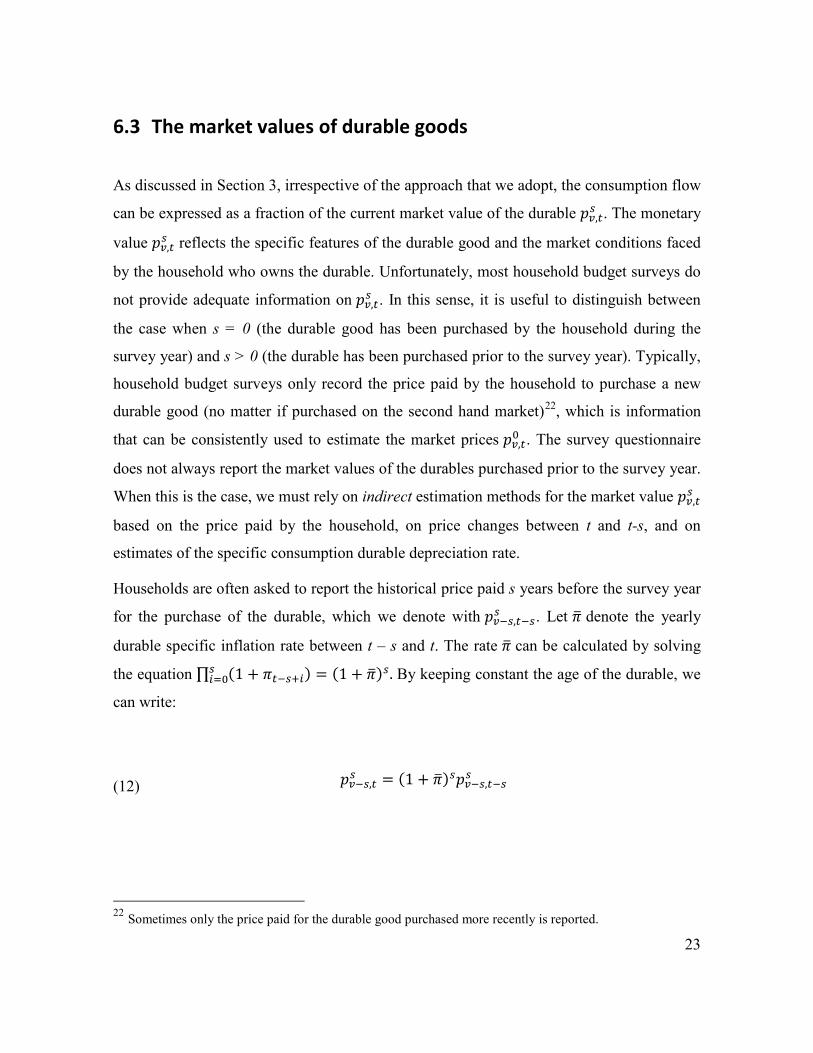
6.3 The market values of durable goods

As discussed in Section 3, irrespective of the approach that we adopt, the consumption flow

can be expressed as a fraction of the current market value of the durable 𝑝𝑝𝑣𝑣,𝑡𝑡𝑠𝑠 . The monetary

value 𝑝𝑝𝑣𝑣,𝑡𝑡𝑠𝑠 reflects the specific features of the durable good and the market conditions faced

by the household who owns the durable. Unfortunately, most household budget surveys do

not provide adequate information on 𝑝𝑝𝑣𝑣,𝑡𝑡𝑠𝑠 . In this sense, it is useful to distinguish between

the case when s = 0 (the durable good has been purchased by the household during the

survey year) and s > 0 (the durable has been purchased prior to the survey year). Typically,

household budget surveys only record the price paid by the household to purchase a new

durable good (no matter if purchased on the second hand market)22, which is information

that can be consistently used to estimate the market prices 𝑝𝑝𝑣𝑣,𝑡𝑡0 . The survey questionnaire

does not always report the market values of the durables purchased prior to the survey year.

When this is the case, we must rely on indirect estimation methods for the market value 𝑝𝑝𝑣𝑣,𝑡𝑡𝑠𝑠

based on the price paid by the household, on price changes between t and t-s, and on

estimates of the specific consumption durable depreciation rate.

Households are often asked to report the historical price paid s years before the survey year

for the purchase of the durable, which we denote with 𝑝𝑝𝑣𝑣−𝑠𝑠,𝑡𝑡−𝑠𝑠𝑠𝑠 . Let 𝜋𝜋� denote the yearly

durable specific inflation rate between t – s and t. The rate 𝜋𝜋� can be calculated by solving

the equation ∏ (1 + 𝜋𝜋𝑡𝑡−𝑠𝑠+𝑐𝑐)𝑠𝑠𝑐𝑐=0 = (1 + 𝜋𝜋�)𝑠𝑠. By keeping constant the age of the durable, we

can write:

(12) 𝑝𝑝𝑣𝑣−𝑠𝑠,𝑡𝑡𝑠𝑠 = (1 + 𝜋𝜋�)𝑠𝑠𝑝𝑝𝑣𝑣−𝑠𝑠,𝑡𝑡−𝑠𝑠

𝑠𝑠

22 Sometimes only the price paid for the durable good purchased more recently is reported. 23

The implementation of equation (12) requires the availability of the time series of some

sort of price index 𝐶𝐶𝐶𝐶𝐶𝐶𝑇𝑇 for T=t-s-1,…,t. If, for instance, the durable good was purchased

10 years prior to the survey year (s = 10), the analyst needs the price indices for the past 11

years. Secondly, equation (12) provides an estimate of 𝑝𝑝𝑣𝑣−𝑠𝑠,𝑡𝑡𝑠𝑠 , that is, of the current value of

a (v–s)-year old durable. However, the durable owned by the household is a v-year old

durable. To estimate 𝑝𝑝𝑣𝑣,𝑡𝑡𝑠𝑠 we need to know the average yearly economic depreciation rate

between age v – s and v. This is what we discuss in the next section.

6.4 The depreciation rate

The depreciation rate measures the loss (or gain) in value that durable goods experience

with age due to their physical deterioration and market value change. The depreciation

pattern of a durable good can be represented in a general way. In order to simplify our

discussion, we shall omit the index s, i.e. we will ignore the purchasing date of the

durable23. Thus, we can write:

(13) 𝑝𝑝1,𝑡𝑡 = (1 − 𝛿𝛿1) 𝑝𝑝0,𝑡𝑡

where 𝑝𝑝0,𝑡𝑡 is the market value of a new durable in t and 𝑝𝑝1,𝑡𝑡 is the market value of a 1-year

old durable in t. The value 𝛿𝛿1 ≤ 1 is the deterioration rate for the first year of life of the

durable. Following the same notation, and with the same interpretation, we can also write:

(14) 𝑝𝑝2,𝑡𝑡 = (1 − 𝛿𝛿2) 𝑝𝑝1,𝑡𝑡

23 In the rest of this section we also assume that delta is unique, for each good, at the national level. In

principle, one can explore the use of different deltas for different regions or population subgroups. To the best

of our knowledge, these possibilities have not been discussed in the literature.

24

Equation (14) expresses the price of the durable good when it turns 2-year old, that is at the

end of the second year, as a fraction of its value when it was 1-year old. Substituting

equation (13) in equation (14) we obtain:

(15) 𝑝𝑝2,𝑡𝑡 = (1 − 𝛿𝛿2)(1 − 𝛿𝛿1) 𝑝𝑝0,𝑡𝑡

Proceeding iteratively one obtains:

(16) 𝑝𝑝𝑣𝑣,𝑡𝑡 = �(1 − 𝛿𝛿𝑐𝑐)𝑣𝑣

𝑐𝑐=1

𝑝𝑝0,𝑡𝑡

According to equation (16) the entire depreciation pattern of the durable good between t–v

and t is described by the sequence {𝛿𝛿𝑐𝑐}𝑐𝑐=1𝑣𝑣 . There are, obviously, many ways of

characterizing this depreciation sequence and they all require different pieces of

information to be implemented. We will here discuss the three most common models that

are found in the literature 24: 1) the geometric depreciation model; 2) the straight line

depreciation and 3) the “light bulb” depreciation. Further, we will suggest a fourth

depreciation model, a mixture of methods 1) and 3), which has the advantage of being

parsimonious in terms of information requirement, and therefore potentially widely

applicable.

6.4.1 The geometric depreciation model

Under the geometric model the depreciation rate is assumed to be constant over time. In

other words, a constant fraction of the value of the durable is lost every year. In equation

(16) this implies that 𝛿𝛿𝑐𝑐 = 𝛿𝛿 for every i:

24 See Hulten and Wykoff (1981, 1996) and Diewert (2003, 2004, 2009). 25

(17) 𝑝𝑝𝑣𝑣,𝑡𝑡 = (1 − 𝛿𝛿)𝑣𝑣 𝑝𝑝0,𝑡𝑡

Equation (17) can be solved with respect to the (unique) depreciation rate 𝛿𝛿:

(18) 𝛿𝛿 = 1 − �𝑝𝑝𝑣𝑣,𝑡𝑡

𝑝𝑝0,𝑡𝑡�

1𝑣𝑣

In equation (18) the estimation of the depreciation rate only requires information on the

market values of homogeneous durable goods of different age. Due to its analytical

simplicity and its empirical robustness, the geometric model is one of the most popular

models25.

6.4.2 The straight line depreciation model

The straight line depreciation model assumes that the economic life of the durable is finite

and that its value follows a linear pattern of depreciation. Let us denote with T the

economic life of the durable: after T years its consumption flow equals zero. According to

the linear depreciation model we have:

(19) 𝑝𝑝𝑣𝑣,𝑡𝑡

𝑝𝑝0,𝑡𝑡= �

𝑇𝑇 − 𝑣𝑣𝑇𝑇

𝑖𝑖𝑖𝑖 𝑣𝑣 ≤ 𝑇𝑇

0 𝑜𝑜𝑡𝑡ℎ𝑒𝑒𝑟𝑟𝑒𝑒𝑖𝑖𝑠𝑠𝑒𝑒

25 See Hulten and Wykoff (1981, 1996) Jorgenson (1996) and Fraumeni (1997). The general conclusion of

the empirical literature on the capital depreciation rate is that the geometric pattern is closer to the actual

pattern than the patterns implied by the straight line and the light bulb depreciation model

26

Hence, it is straightforward to show that:

(20) 𝛿𝛿𝑐𝑐 = �1

𝑇𝑇 − 𝑖𝑖𝑖𝑖𝑖𝑖 𝑖𝑖 < 𝑇𝑇

1 𝑜𝑜𝑡𝑡ℎ𝑒𝑒𝑟𝑟𝑒𝑒𝑖𝑖𝑠𝑠𝑒𝑒

where 𝛿𝛿𝑐𝑐 is the depreciation rate for the year i of the economic life of the durable good.

Equation (20) shows that, unlike in the geometric depreciation method, the depreciation

rate here is not constant over time. This implies that in order to implement the user cost

formula we need to calculate a vintage-specific depreciation rate 26. Also note that the

implementation of the straight line depreciation model requires the knowledge of T, which

requires an estimate of the economic life for each and every durable good owned by the

households.

Deaton and Zaidi (2002) assume that the age of the durable goods is uniformly distributed.

Accordingly, 2𝑇𝑇� is an estimator of the maximum economic life of the durable, where 𝑇𝑇� is

the average life of the durable calculated form the data recorded in the survey. An

alternative consists in using some outlier-resistant statistics computed over the set of the

most long-lived goods in the sample: one possibility, for instance, is the 95th percentile of

the sample distribution of the ages of the durable good.

6.4.3 The light bulb depreciation model

The light bulb depreciation model, also known as the “one-hoss shay” model, is the

simplest among the depreciation models. The idea is that the durable maintains its

efficiency and value along all its economic life and ceases to work, like a bulb, after T

years. Accordingly, the consumption flow, as measured by the user cost, is constant over

26 For an application of the linear depreciation model see Diewert (2003).

27

the entire economic life of the durable. Let us define 𝑈𝑈𝑡𝑡 = 𝑈𝑈𝐶𝐶𝑡𝑡/(1 + 𝑖𝑖𝑡𝑡) as the user cost of

the durable evaluated at the beginning of period t. Equation (4) allows us to write:

(21) 𝑈𝑈𝑡𝑡 = 𝑝𝑝𝑣𝑣,𝑡𝑡𝑠𝑠 +

(1 + 𝜋𝜋𝑡𝑡)(1 + 𝑖𝑖𝑡𝑡)

𝑝𝑝𝑣𝑣+1,𝑡𝑡𝑠𝑠

If 𝑈𝑈𝑡𝑡 = 𝑈𝑈� is a constant for 𝑣𝑣 < 𝑇𝑇, then equation (21) can be rewritten as follows:

(22) 𝑝𝑝𝑣𝑣,𝑡𝑡𝑠𝑠 = 𝑈𝑈� + 𝛾𝛾𝑡𝑡𝑝𝑝𝑣𝑣+1,𝑡𝑡

𝑠𝑠

where 𝛾𝛾𝑡𝑡 = (1+𝜋𝜋𝑡𝑡)(1+𝑐𝑐𝑡𝑡) . We also assume 𝛾𝛾𝑡𝑡 < 1, i.e. that the real interest rate is always strictly

positive.

Each durable goods maintains its efficiency for T periods and then ceases to function.

Precisely at that time, 𝑝𝑝𝑇𝑇,𝑡𝑡𝑠𝑠 = 0. Substituting iteratively the RHS term in equation (22) we

obtain:

(23) 𝑝𝑝𝑣𝑣,𝑡𝑡𝑠𝑠 = 𝑈𝑈�[1 + 𝛾𝛾𝑡𝑡 + 𝛾𝛾𝑡𝑡2 … . +𝛾𝛾𝑡𝑡𝑇𝑇−1−𝑣𝑣] = 𝑈𝑈� �

1 − 𝛾𝛾𝑡𝑡𝑇𝑇−𝑣𝑣

1 − 𝛾𝛾𝑡𝑡�

By using equation (18) we obtain the final formula for the “light bulb” depreciation rates:

(23) 𝛿𝛿𝑣𝑣𝑡𝑡 = 1 − �1 − 𝛾𝛾𝑡𝑡𝑇𝑇−1−𝑣𝑣

1 − 𝛾𝛾𝑡𝑡𝑇𝑇−𝑣𝑣�

It should be observed that in order to estimate the depreciation rate for the user cost formula

we need to know the “duration” T of the durable, i.e. its economic life, and the parameter

28

𝛾𝛾𝑡𝑡 that depends on the period t asset specific inflation rate 𝜋𝜋𝑡𝑡 and on the nominal interest

rate 𝑖𝑖𝑡𝑡. If we assume that 𝛾𝛾𝑡𝑡 is constant over time the depreciation rate only varies with v,

i.e. with the vintage of the durable27.

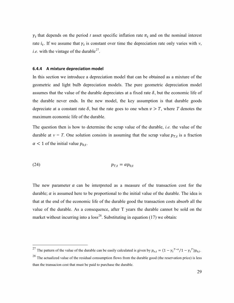
6.4.4 A mixture depreciation model

In this section we introduce a depreciation model that can be obtained as a mixture of the

geometric and light bulb depreciation models. The pure geometric depreciation model

assumes that the value of the durable depreciates at a fixed rate 𝛿𝛿, but the economic life of

the durable never ends. In the new model, the key assumption is that durable goods

depreciate at a constant rate 𝛿𝛿, but the rate goes to one when 𝑣𝑣 > 𝑇𝑇, where T denotes the

maximum economic life of the durable.

The question then is how to determine the scrap value of the durable, i.e. the value of the

durable at v = T. One solution consists in assuming that the scrap value 𝑝𝑝𝑇𝑇,𝑡𝑡 is a fraction

𝛼𝛼 < 1 of the initial value 𝑝𝑝0,𝑡𝑡.

(24) 𝑝𝑝𝑇𝑇,𝑡𝑡 = 𝛼𝛼𝑝𝑝0,𝑡𝑡

The new parameter 𝛼𝛼 can be interpreted as a measure of the transaction cost for the

durable; 𝛼𝛼 is assumed here to be proportional to the initial value of the durable. The idea is

that at the end of the economic life of the durable good the transaction costs absorb all the

value of the durable. As a consequence, after T years the durable cannot be sold on the

market without incurring into a loss28. Substituting in equation (17) we obtain:

27 The pattern of the value of the durable can be easily calculated is given by 𝑝𝑝𝑣𝑣,𝑡𝑡 = (1 − 𝛾𝛾𝑡𝑡𝑇𝑇−𝑣𝑣 1 − 𝛾𝛾𝑡𝑡𝑇𝑇⁄ )𝑝𝑝0,𝑡𝑡. 28 The actualized value of the residual consumption flows from the durable good (the reservation price) is less

than the transacion cost that must be paid to purchase the durable. 29

(25) 𝛼𝛼𝑝𝑝0,𝑡𝑡 = (1 − 𝛿𝛿)𝑇𝑇 𝑝𝑝0,𝑡𝑡

and solving with respect to 𝛿𝛿 we can write:

(26) 𝛿𝛿 = 1 − 𝛼𝛼1𝑇𝑇

Equation (26) compares with equation (18). The advantage of equation (26) is that it does

not require information on the current market prices of durable goods with different

manufacturing years. This facilitates tremendously its implementation, both when data are

relatively abundant, and even more so when the survey only provides an inventory of the

durable goods owned by the households. A drawback is that the estimate of the

depreciation rate 𝛿𝛿 depends on the parameter 𝛼𝛼, which is arbitrarily chosen by the analyst.

In fact, it can be shown that the consumption flow from the durable is quite insensitive to

choice of alpha. Equation (26) can be substituted in equation (10) and the elasticity of the

consumption flow with respect to alpha 𝜂𝜂𝐶𝐶𝐶𝐶 𝛼𝛼⁄ can be easily calculated:

(27) 𝜂𝜂𝐶𝐶𝐶𝐶𝑡𝑡 𝛼𝛼⁄ = 1𝑇𝑇 �𝑟𝑟𝑡𝑡 + 1− 2𝛼𝛼

1𝑇𝑇

𝑟𝑟𝑡𝑡 + 1−𝛼𝛼1𝑇𝑇� = 1

𝑇𝑇ℎ(𝛼𝛼)

where ℎ(𝛼𝛼) is always less than one and is a decreasing function of 𝛼𝛼. Hence the elasticity

of the consumption flow with respect to 𝛼𝛼 is always less than one and tends to zero as the

age of the durable tends to infinity. To get a sense of the magnitude of 𝜂𝜂𝐶𝐶𝐶𝐶 𝛼𝛼⁄ , assume a

conservative scenario where 𝑇𝑇 = 2 , 𝛼𝛼 = 0.10 and 𝑟𝑟𝑡𝑡 = 0.05; under this assumption the

elasticity 𝜂𝜂𝐶𝐶𝐶𝐶 𝛼𝛼⁄ = 0.28, that is a one percent increase in 𝛼𝛼 is associated with a 0.28 percent

increase in the consumption flow. Ceteris paribus, if 𝑇𝑇 = 25, 𝜂𝜂𝐶𝐶𝐶𝐶 𝛼𝛼⁄ = −0.22. Again, the

consumption flow is anelastic to 𝛼𝛼. 30

Figure 2 – Depreciation models compared

Source: our elaboration.

Figure 2 compares the four depreciation models described in this section. On the vertical

axis, the initial value of the durable good is normalized to one. We assume that the

geometric depreciation rate is 10% and that the economic life T is equal to 25 years

(empirically, these are reasonable assumptions for many consumer durables). The dashed

line describes the pattern of the straight line model, while the blue line describes the pattern

of the bulb light model. The geometric depreciation pattern is represented by the black solid

line. The green and the red lines describe the mixture model under the assumption that

𝛼𝛼 = 5% and 𝛼𝛼 = 10%, respectively.

31

6.4.5 Econometric models

A depreciation rate gives the percentage change of the market value of a durable good

between two subsequent years. In principle, depreciation rates can be calculated directly

from the empirical age-price curves for each durable good. In practice, however, lack of

adequate data prevent the analyst from drawing complete age profiles for most durable

goods and, as a consequence, to estimate the required depreciation rates 29. It is then

necessary to estimate the age-price profile by using an econometric model.

Studying the economic depreciation of capital assets Hulten and Whykoff (1981)

introduced an econometric model that encompasses all the theoretical depreciation models

described in sections 6.4.1-6.4.330. Let 𝑝𝑝𝑐𝑐 be the observed market price of an asset of age 𝑣𝑣𝑐𝑐

in year 𝑡𝑡𝑐𝑐. Then, the Box-Cox model for the used asset price is:

(28) �̂�𝑝𝑐𝑐 =∝ +𝛽𝛽𝑣𝑣�𝑐𝑐 + 𝛾𝛾�̂�𝑡𝑐𝑐 + 𝑢𝑢𝑐𝑐

where

�̂�𝑝𝑐𝑐 =𝑝𝑝𝑐𝑐𝜃𝜃1 − 1𝜃𝜃1

; 𝑣𝑣�𝑐𝑐 =𝑣𝑣𝑐𝑐𝜃𝜃2 − 1𝜃𝜃2

; �̂�𝑡𝑐𝑐 =𝑡𝑡𝑐𝑐𝜃𝜃3 − 1𝜃𝜃3

29 As observed by Hulten and Wykoff (1981a, 1981b), there is also a problem of censoring. The used price

sample contains only the price of the “survived” durables and they provide a biased estimate of the average

value of a specific vintage. A possible correction for censoring consists in multiplying the prices of surviving

assets of each vintage by the age dependent probabilities of survival. Jorgenson (1996) shows that this

correction has a relevant impact on depreciation rate estimates. Another possible source of bias depends on

the fact that the equilibrium prices in second hand markets might be largely affected by adverse selection

phenomena (Akerlof, 1970). 30 An alternative econometric model was proposed by Oliner (1993) who augmented the standard linear

regression model with polynomial components for 𝑣𝑣𝑐𝑐 and 𝑡𝑡𝑐𝑐. Micro-Economic Analysis Division of Canada

(2007) has carried out a variety of other estimation exercises based on survival econometric models.

32

and 𝑢𝑢𝑐𝑐 ∼ 𝑁𝑁(0,𝜎𝜎2). The parameter vector 𝜽𝜽 = (𝜃𝜃1,𝜃𝜃2,𝜃𝜃3) identifies the specific functional

form of the Box-Cox power transformation that corresponds to the theoretical depreciation

models discussed above. In particular, for 𝜽𝜽 = (0,1,1) equation (28) takes the semi-log

form that corresponds to the geometric depreciation pattern31. When 𝜽𝜽 = (1,1,1) we obtain

the linear depreciation pattern, while 𝜽𝜽 = (1,3,1) identifies the light bulb model.

In the absence of reliable data on used asset prices, the assumption of a geometric

depreciation pattern can be used to derive an alternative estimation procedure:

(29) 𝛿𝛿 =𝑝𝑝𝑣𝑣 − 𝑝𝑝𝑣𝑣+1

𝑝𝑝𝑣𝑣; 𝑣𝑣 = 0,1, … . . ,𝑇𝑇− 1

where 𝑝𝑝𝑣𝑣 is the vintage v asset price (we omit here the temporal index t) and T is the

expected economic life of the asset. From equation (29) we derive:

(30) 𝑇𝑇𝛿𝛿 = �𝑝𝑝𝑣𝑣 − 𝑝𝑝𝑣𝑣+1

𝑝𝑝𝑣𝑣

𝑇𝑇−1

𝑣𝑣=0

Equation (30) can be rewritten as follows:

(31) 𝛿𝛿 = ��𝑝𝑝𝑣𝑣 − 𝑝𝑝𝑣𝑣+1

𝑝𝑝𝑣𝑣

𝑇𝑇−1

𝑣𝑣=0� 𝑇𝑇� = 𝐷𝐷𝐷𝐷𝑅𝑅

𝑇𝑇

where DBR is known in the literature as the “declining balance rate”. The larger is the

expected service life T of the durable, the higher must be the declining balance rate

31 See also Jorgenson (1996)

33

consistent with a given geometric depreciation rate32. The idea of the method is that of

estimating directly DBR for all the assets for which there are reliable information on prices

and then to use these estimates to calculate, by means of eq. (31), the depreciation rate for

which there are only information about the expected economic life of the asset. This

“second best” estimation procedure that was firstly proposed by Hulten and Wykoff

(1981a, 1981b, 1996) is the one mainly adopted by the Bureau of Economic Analysis to

produce its official comprehensive table of depreciation rates33 (Fraumeni, 1997, BEA,

2003).

7 Conclusions

The estimation of the value of the flow of services from durable goods is a relevant issue in

many areas of economic analysis, from national accounting to price index theory, as well as

in welfare analysis. In this paper the focus has been on the treatment that consumer durable

goods must receive in the process of constructing a welfare aggregate. The economic

literature is relatively abundant in theoretical studies focused on the economic depreciation

of assets. The single most debated issue refers to the measurement of capital and

investment decisions. In contrast, the questions of economic depreciation of consumer

durable goods and the impact that different approaches have on the measurement of welfare

at the individual- or household-level have remained largely unexplored issues.

A general conclusion of the literature is that the user cost approach (section 3.3) is the most

appropriate pricing concept to evaluate the flow of services from durable assets. We also

found a broad consensus on the fact that the geometric depreciation model (section 6.4.1) is

the most empirically robust as well as theoretically consistent depreciation model for

32 Equation (31) is clearly an approximated formula. In the geometric depreciation model there is no ending

date for the capital asset. 33 According to the most recent BEA estimates, the DBR values range from 0.89 to 2.27

(www.bea.gov/national/pdf/BEA_depreciation_rates.pdf).

34

capital assets. Our analysis supports the fact that most of the advantages that hold true for

capital goods, broadly defined, also hold true for consumer durable goods. Alternative

approaches, like the acquisition approach or the rental equivalence approach, imply a

higher risk of affecting in undesired ways the distribution of the welfare aggregate, and

more generally welfare comparisons.

The second finding, relating to the advantages of the geometric depreciation model, is more

controversial for two reasons. The empirical evidence in favor of the geometric model is

based on capital assets and not on consumer durables. Extending the same line of argument

to consumer durables is not straightforward. Secondly, the lack of adequate data is often

responsible for insurmountable difficulties that prevent the analyst from estimating the

geometric depreciation rate for consumer durable goods. We suggested a new depreciation

model that preserves the basic structure of the geometric model, but relies on a more

parsimonious set of statistical information.

The main deficiency in the literature reviewed in this paper is that it fails to assess the

impact of the consumption flow from durable goods on the measurement of welfare and its

distribution. We are not aware of studies that come up with an evaluation of the impact on

poverty and inequality measures of including (excluding) the consumption flow in (from)

the welfare aggregate. Nor are we aware of studies that report the sensitivity of the welfare

distribution to different estimation methods of estimating the consumption flow. This adds

uncertainty when it comes to advising on the “best method” to use in practice, and to

designing guidelines for the construction of the welfare aggregate. Further research is badly

needed in this area.

35

References

Akerlof, G. (1970), The Market for Lemons, Quarterly Journal of Economics, 488-500

Alchian, A. and B. Klein, (1973) On a Correct Measure of Inflation, Journal of Money Credit and Banking, Vol. 5, 173-191.

Amendola, N. and G. Vecchi (2010), "Setting a Poverty Line for Iraq", in Confronting Poverty in Iraq: an Analytical Report on the Living Standard of the Iraqi Population, The World Bank.

Arrow, K. J. (1971) Essays on the Theory of Risk Bearing. Chicago: Markham Publishing.

Australian Bureau of Statistics (2012), Household Expenditure Survey and Survey of Income and Housing, User Guide, Australia 2009–10, ABS, Canberra.

Australian Bureau of Statistics (2013), Household Income and Income Distribution, Australia, 2011-12. ABS, Canberra.

Bureau of Economic Analysis (BEA), (2003), Fixed Assets and Consumer Durable Goods in the United States, 1925-97, U.S. Department of Commerce

Citro, C.F. and R.T. Michael (eds.) (1995), Measuring Poverty. A New Approach. Washington DC: National Academy Press.

Deaton, A. (1997), The Analysis of Household Surveys. A Microeconomateric Approach to Development Policy. The John Hopkins University Press.

Deaton A. and J. Muellbauer (1980), Economics and Consumer Behavior, Cambridge University Press.

Deaton A. and S. Zaidi (2002), “Guidelines for Constructing Consumption Aggregates for Welfare Analysis.” Living Standards Measurement Study Working Paper n. 135. The World Bank, Washington, DC.

Department for Work and Pensions (2013), Households Below Average Income. An analysis of the income distribution 1994/95 – 2011/12, June 2013 (United Kingdom)

Diewert, W. E. (2002) ‘‘Harmonized Indexes of Consumer Prices: Their Conceptual Foundations’’, in Swiss Journal of Economics and Statistics, Vol. 138, No. 4.

Diewert, W. E. (2003), “Measuring Capital”, NBER Working Paper, n. 9526

Diewert, W. E. (2004), “Durables and User Costs” in ILO, Consumer Price Index Manual: Theory and Practice, chapter 23, ILO/IMF/OECD/UNECE/Eurostat/World Bank.

Diewert, W. E. (2009), “Durables and Owner-Occupied Housing in a Consumer Price Index” in W. E. Diewert , J.S. Greenlees and C.R. Hulten (eds.), Price Index Concepts and Measurements, University of Chicago Press.

36

Fellegi, I.P. (1997), “On poverty and low income”, available here: http://www.statcan.gc.ca/pub/13f0027x/13f0027x1999001-eng.htm.

Fisher, I (1911), The purchasing power of money, Its Determination and Relation to Credit, Interest, and Crises. New Yoor: The McMillan Co.

Fraumeni, B. (1997) ”Measurement of Depreciation in the US. National Income and Wealth Accounts.” Survey of Current Business. US, vol 77 (7), 7 – 23

Garner, T. and R. Verbrugge (2007), “The Puzzling Divergence of U.S. Rents and User Costs, 1980-2004: Summary and Extensions”, BLS Working Papers, WP n.409

Gillingham R. (1983), “Measuring the Cost of Shelter for Homeowners: Theoretical and Empirical Considerations”, The Review of Economics and Statistics, (65)2: 254-65.

Goodhart, C. (2001), “What Weight Should be given to Asset Price in Measurement of Inflation?”, The Economic Journal, Vol. 111, 335-356.

Government of India (2007) “Poverty Estimates for 2004-05”. New Delhi.

Hicks, J.R. (1955), Capital and Growth, Oxford Clarendon Press

Hulten, C. R. (1990), “The measurement of capital”. In Fifty years of economic measurement, ed. E. R. Berndt and J. E. Triplett, 119– 58. Chicago: University of Chicago Press.

Hulten, C. R. and F. Wykoff (1981), “The measurement of Economic Depreciation” in C. R. Hulten eds, Inflation and Taxation of Income from Capital, Washington DC

Hulten, C. R. and F. Wykoff (1996), “Issues in the Measurement of Economic Depreciation: Introductory Remarks”, Economic Inquiry, 34 (1): 10– 23.

ILO (2004), Consumer price index manual: Theory and Practice. Geneva, International Labour Office, 2004

Jalava, J and Kavonius, K (2009), “Measuring The Stock of Consumer Durables and its Implications for Euro Area Savings Ratios”, Review of Income and Wealth, 55, 1.

Jorgenson, D. W. (1963), “Capital Theory and Investment Behaviour”, American Economic Review, 53: 247-259.

Jorgenson, D. W. (1973), “The economic Theory of Replacement and Depreciation”. In Econometrics and Economic Theory, ed. W. Sellekaerts, 189– 221. New York: Macmillan.

Jorgenson D. W. and S. Lanfeld (2006) “Blueprint for Expanded and Integrated U.S. Accounts Review, Assessment, and Next Steps”, in A New Architecture for the U.S. National Accounts, Dale W. Jorgenson, J. Steven Landefeld, and William D. Nordhaus (eds.), The University of Chicago Press Chicago and

37

Koumanakos, P. and J.C. Hwang, (1988). The Forms and Rates of Economic Depreciation, The Canadian Experience. Presented at the 50th anniversary meeting of the Conference on Research in Income and Wealth, Washington, DC, May 1988.

Katz, A. J. (1983), “Valuing the services of consumer durables”, Review of Income and Wealth, 29 (4): 405– 27.

Lanjouw, P (2009), “Constructing a Consumption Aggregate for the Purpose of Welfare Analysis: Principles, Issues and Recommendations Arising from the Case of Brazil”.

Meyer, B. D. and J.X. Sullivan (2011), “Consumption and Income Poverty over the Business Cycle”, NBER Working Paper No. 16751.

Micro-Economic Analysis Division (2007), “Depreciation Rates for the Productivity accounts”, The Canadian Productivity Review.

Moulton, B.R. (2004), “The System of National Accountsfor the New Economy: What Should Change?”, Review of Income and Wealth, 50 (2): 261-278.

Murphy, B., X. Zhang, and C. Dionne (2010), “Revising Statistics Canada's Low Income Measure (LIM)”, Income Research Paper Series, Statistics Canada, Income Statistics Division.

Murphy, B., X. Zhang, and C. Dionne (2012), “Low Income in Canada: a Multi-line and Multi-index Perspective”, Income Research Paper Series, Statistics Canada, Income Statistics Division.

OECD (2009), Manual: Measuring Capital, Second Edition OECD, Paris,

OECD (2013), OECD Framework for Statistics on the Distribution of Household Income, Consumption and Wealth, OECD Publishing.

Offer, A. (2005), The Challenge of Affluence. Self-Control and Well-Being in the United States and Britain since 1950. Oxford University Press.

Oliner, S. D. (1993) ”Constant-Quality Price Change, Depreciation, and Retirement of Mainframe Computers,“ in Price Measurements and Their Uses, edited by M. F. Foss, M. E. Manser, and A. H. Young. Chicago: University of Chicago Press.

Slesnik, D.T. (2000), Consumption and Social Welfare: Living Standards and Their Distribution in the United States, Cambridge University Press.

System of National Accounts (2008), Commission of the European Communities, International Monetary Fund, United Nations, World Bank, Brussels/Luxembourg, New York, Paris, Washington, DC, 1993.

Young, A.S. (2005), “Some Uncertainties in Household Consumption Expenditure Statistics”, mimeo (www.statssa.gov.za/commonwealth/presentations/Paper_young.pdf).

38