Durham E-Theses

Three dimensional frequency-domain solution method

for unsteady turbomachinery �ows

Vasanthakumar, Parthasarathy

How to cite:

Vasanthakumar, Parthasarathy (2003) Three dimensional frequency-domain solution method for unsteady

turbomachinery �ows, Durham theses, Durham University. Available at Durham E-Theses Online:http://etheses.dur.ac.uk/3089/

Use policy

The full-text may be used and/or reproduced, and given to third parties in any format or medium, without prior permission orcharge, for personal research or study, educational, or not-for-pro�t purposes provided that:

• a full bibliographic reference is made to the original source

• a link is made to the metadata record in Durham E-Theses

• the full-text is not changed in any way

The full-text must not be sold in any format or medium without the formal permission of the copyright holders.

Please consult the full Durham E-Theses policy for further details.

Academic Support O�ce, Durham University, University O�ce, Old Elvet, Durham DH1 3HPe-mail: e-theses.admin@dur.ac.uk Tel: +44 0191 334 6107

http://etheses.dur.ac.uk

2

I!Jfj ~fti~:6~ School of Engineering

THREE DlM~ENSIONAL FREQUENCY-DOMAIN SOLUTION METHOD FOR UNSTEADY TURBOMACIDNERY FLOWS

Parthasarathy Vasanthakumar

The copyright of this thesis rests with the author.

No quotation from it should be published without

his prior written consent and information derived

from it should be acknowledged.

~t:T> . .

- ' ' 2 9 .JAN zorn

A thesis submitted for the degree of Doctor of Philosophy

School ofEngineering University of Durham

2003

Abstract

The three-dimensional calculation of unsteady flows is increasingly gammg

importance in the prediction of turbomachinery flow problems. A three-dimensional

Euler/Navier-Stokes solver incorporating the time-linearized method and the

nonlinear harmonic method in the frequency domain has been developed for

predicting unsteady turbomachinery flows.

In the time-linearized method, the flow is decomposed into a steady part and a

harmonic perturbation part. Linearization results in a steady flow equation and a time­

linearized perturbation equation. A pseudo-time time-marching technique is

introduced to time-march them. A cell centred finite volume scheme is employed for

spatial discretization and the time integration involves a four stage Runge Kutta

scheme. Nonreflecting boundary conditions are applied for far field boundaries and a

slip wall boundary condition is used for Navier-Stokes calculations. In the nonlinear

harmonic method, the flow is assumed to be composed of a time-averaged part and an

unsteady perturbation part. Due to the nonlinearity of the unsteady equations, time­

averaging produces extra unsteady stress terms in the time-averaged equation which

are evaluated from unsteady perturbations. While the unsteady perturbations are

obtained from solving the harmonic perturbation equation, the coefficients of

perturbation equations come from the solution of time-averaged equation and this

interaction is achieved through a strong coupling procedure. In order to handle flows

with strong nonlinearity, a cross coupling of higher order harmonics through a

harmonic balancing technique is also employed. The numerical solution method is

similar to that used in the time-linearized method.

The numerical validation includes several test cases involving linear and nonlinear

unsteady flows with specific attention to flows around oscillating blades. The results

have been compared with other well developed linear methods, nonlinear time­

marching method and experimental data. The nonlinear harmonic method is able to

predict strong nonlinearities associated with shock oscillations well but some

limitations have also been observed. A three-dimensional prediction of unsteady

viscous flows through a linear compressor cascade with 3D blade oscillation,

probably the first of its kind, has shown that unsteady flow calculation in the

frequency domain is able to predict three-dimensional blade oscillations reasonably

well.

Declaration

This thesis is based on research carried out by the author during the period January 1999- September 2002 at University of Durham, under the supervision of Prof. Li He. No part of it has previously been submitted for any degree, either at this university or anywhere else.

11

Acknowledgement

During the course of this research programme I have had the pleasure of interacting

with many people and needless to say, I have received help and support from various

quarters in this period.

I would like to thank my supervisor, Prof. Li He, for his supervision, guidance and

support throughout the course of this research programme and particularly for

providing critical insights to problem solving. I would like to extend my thanks to Tie

Chen for his help during the code development stages. I would also like to thank Hui

Yang for providing the 3D experimental data. Thanks are also due to Haidong, Yun,

Kenji and Stuart for all those stimulating discussions.

This research programme was sponsored by Alstom Power and I wish to acknowledge

Roger Wells, Yangshen Li and Wei Ning for many helpful discussions. A part of the

tuition fee for this programme was provided by the ORS award for three years.

111

Abstract

Declaration

Acknowledgement

Contents

Nomenclature

Chapter 1 Kntroductiorn

1.1 General Background

Coll1lttell1ltts

1.2 Aerodynamic Damping

1.3 Some Relevant Parameters

1.3.1 Reduced Frequency

1.3.2 Inter-Blade Phase Angle

1.4 Relevance ofThree-Dimensional Computation

1.5 Overview ofThesis

Chapter 2 Review of lLiteratUllre

2.1 Computational Methods for Unsteady Flows in Turbomachinery

2.2 Nonlinear Time-Marching Method

2.2.1 Blade Row Interaction

2.2.2 Flutter

2.3 Time-Linearized Harmonic Method

2.4 Nonlinear Harmonic Method

Chapter 3 Unsteadiness and lFnow Nonlinearity

3.1 Unsteady Flow and the Concept of Averaging

3.1.1 Random Unsteadiness and Reynolds Averaging

3.2 Nonlinearity in Deterministic Unsteady Flow

3.2.1 Time-Averaging and Deterministic Stresses

Chapter 4 lLinear Harmonic Method!

4.1 Governing Equations

4.2 Time-Linearization

4.3 Numerical solution Method

4.3.1 Pseudo Time Dependence and Numerical Discretization

IV

11

Ill

IV

VI

1

1

3

5

5

6

7

9

10

10

11

12

15

17

19

23

23

24

27

28

31

31

32

36

36

4.3.2 Boundary Conditions

Chapter 5 Nonlinear Harmonic Method

5.1 Time-Averaging and Incorporating Nonlinearity

5.2

5.3

5.3.1

5.4

First Harmonic Perturbation Equation

Inclusion of Higher Order Harmonic Perturbations

Harmonic Balance Method

Numerical Discretization

39

45

45

49

54

55

59

5.5 Coupling Between Time-Averaged Flow and Unsteady Perturbation 60

Chapter 6 Two-Dimensional Results and Discussion 62

6.1 Oscillating Flat Plate Cascade 62

6.2 High Frequency Incoming Wakes

6.3 Oscillating Turbine Cascade (Fourth Standard Configuration)

6.4 Inviscid Transonic Unsteady Channel Flow

64

66

68

6.5 Inlet Distortion Through a Transonic Axial Flow Fan Rotor 72

Chapter 7 Three-Dimensional Results and Discussion 75

7.1 Validation of Three-Dimensional Euler Sol uti on 7 5

7.2 Unsteady Viscous Flow Through an Oscillating Compressor Cascade 77

Chapter 8 Conclusions and Suggestions 82

8.1 Linear Harmonic Method 82

8.2 Nonlinear Harmonic Method

8.3 Suggestions for Future Work

References

Figures

v

83

85

87

Symbol

A

c c

e

F

G

H

k

L

M

N

p

Po r

Re

s T

f

t'

u u

v v

Nomenclature

Computational cell face area; Diverging channel height

Amplitude of oscillation

Blade chord

Local speed of sound

Friction coefficient

Pressure coefficient

Fluid internal energy

Flux vector in the x direction

Flux vector in the e direction

Flux vector in the r direction; Blade height

Reduced frequency; Coefficient of heat conductivity

Reference length

Mach number

Blade number; Wave number; Number of perturbations

Static pressure

Total pressure

Radius; Radial coordinate

Reynolds number

Source term vector; Blade Span; Blade Spacing

Temperature; Time

Time

Pseudo time

Conservative variables vector

Velocity in the x direction

Grid moving velocity in the x direction

Reference velocity

Computational cell volume

velocity in the e direction

VI

w

X

y p

¢>

(J

r

J1

p

OJ

Subscript

I

t

x,B,r

exit

in!

ref

wake

Superscript

I

u

Grid moving velocity in the (J direction; Blade row rotating speed

Velocity in the r direction

Grid moving velocity in the r direction

Axial coordinate

Blade pitch; Incoming wake pitch

Phase angle

Tangential coordinate

Stagger angle; Specific heat ratio

Kinematic viscosity

Density

Inter-blade Phase Angle

Angular frequency

Complex conjugate

Inlet

Laminar

Turbulent

Variables in the x, (J and r directions respectively

Variable at exit

Variable at inlet

Reference quantity

Variable in wake

Time-averaged quantity

Unsteady perturbation

Steady state quantity

Complex amplitude of perturbation

Lower

Upper

Vll

Clhla pten- ]_

ITrrn tn-odl u.n cti o rrn

Ll Generan lBackgroam.dl

Turbomachinery flows are highly complex, three-dimensional and unsteady. New

blade designs are becoming more three-dimensional with large amounts of twist and

sweep and with very small inter-blade spacing. As the aerodynamic loading increases,

the evaluation of unsteady loading and blade stress levels becomes more important in

the design process. The aeromechanical behaviour of fans, compressors and turbines

is strongly dependent on the unsteady aerodynamic behaviour of the blade rows.

Aerodynamics related blade vibration is an undesirable consequence of the unsteady

flow process in an axial flow turbomachine that can lead to structural failure of the

blading. The vulnerability of turbomachines to vibration is not surprising in view of

the large gas loads and the small amount of mechanical damping and the high load at

the rotor root arising from the centrifugal loading.

Flutter and forced response are the two categories of aerodynamically induced blade

vibrations. Flutter is a dynamic aeroelastic instability, in which the aerodynamic

forces that sustain the blade motion are regarded as being solely dependent on that

motion. The flow perturbation due to motion of internal boundaries produces the

physical mechanism for blade flutter. The blade motion, however, causes unsteady

forces to act upon the blade surface, and it is the coupling of these forces with the

existing blade mode that results in the phenomenon of blade flutter. It is the phase

relationship between the blade motion and the unsteady forces induced that

determines the onset of flutter. Given the correct phase relation, the unsteady forces

will do work on the blade and flutter will commence. Under other conditions, work

will be done by the blade on the surrounding fluid, and damping of the blade vibration

will take place. Blade flutter modes can occur in two different ways; the bending

mode where the tip of the blade vibrates around the axial direction and the torsion

mode where the blade rotates around the spanwise direction. Nevertheless, it is now

widely accepted that the turbomachinery blade flutter tends to be a single mode

phenomenon, unlike the wing flutter in which bending and torsion modes couple

together. The turbomachine blade is much stiffer than the airplane wing since the

mass ratio of blade/fluid is considerably larger. The unsteady aerodynamic forces are

generally not large enough to significantly alter the natural mode shapes and

frequencies of the system at the rotational speed of interest. Therefore, the self-excited

vibrations are normally not of the coalescence mode type.

Flutter is primarily seen in fans, front and middle compressor blades, and high aspect

ratio low pressure turbine stages. The types of flutter observed in turbomachinery

blading are shown on an operating map of a compressor in Fig. 1.1. Flutter in

compressors is often comparatively ill defined, occurring at frequencies that are not

multiples of engine order and at different places in the operating map of the

compressor. Flutter rarely occurs at or near the design point. The most common type

is high operating line flutter, which is usually called stall flutter. This is seen in fans

and frontal compressor stages. The next most common type of flutter is supersonic

unstalled flutter, which is commonly seen in shrouded fans. Choke flutter is a less

common, low operating line, type of flutter experienced by middle and rear

compressor stages (Kielb, 1999). Flutter sometimes occurs on only a few blades in a

row with different amplitudes on the individual blades, but as the amplitude rises the

flutter tends to be more coherent to involve all the blades at a common frequency with

a fixed phase angle between the motions of adjacent blades.

In forced vibration, the aerodynamic forces that excite the motion are independent of

that motion. The circumferential asymmetry in the mean flow gives rise to the forced

response of the blading (Sisto, 1977). Flutter can occur over a wide range of operating

condition while forced vibration can occur when a periodic aerodynamic excitation,

with frequency close to a structural system natural frequency acts on the blades in a

given row. Such excitations arise from inlet or exit flow non-uniformities and the

aerodynamic interactions that occur between a given blade row and neighbouring

blade rows. The flow non-uniformities include variations in total pressure, total

temperature and static pressure at inlet and variations in static pressure at the exit. The

blade row interactions include potential flow and wake interactions. The potential

flow interaction is associated with static pressure variation on a given row from

upstream and downstream and wake interaction is the effect on the flow through

wakes shed by upstream rows (Verdon, 1993 ). The potential interaction decays

exponentially with an increase in the axial gap between the blade rows, whereas the

2

wake interaction can propagate several blade rows downstream. For forced vibration

almost all the sources must be at harmonics of the rotational frequency of the rotor

itself. The Campbell diagram, Fig. 1.2, presents the change in blade vibration

frequency as the rotational speed of the machine increases, together with the

corresponding engine order frequencies. Integral order vibrations correspond to

vibrations when the blade vibration frequency lies close to one of the engine orders.

Whether in flutter or forced vibration the blades vibrate in their natural modes at their

natural frequencies. The natural frequencies can be changed by changing the design of

the blade, but once the blade is made the natural frequencies are essentially fixed

parameters for the aerodynamic investigation.

The ability to predict the aeromechanical response of blades arising out of flutter and

forced response is critical to further improvement in the performance of

turbomachinery and requires a detailed understanding of flows in cascades. Since

cascade tests of transonic flows are complicated and very expensive, numerical

simulation is a very useful and practical tool to study this phenomenon. The

development of computational fluid dynamics has provided an opportunity to

formulate these tools. Accurate and efficient aerodynamic analyses are needed to

determine the unsteady blade loads for the simulation of nonlinear viscous unsteady

flows. There are two different types of analysis namely time domain analysis and

frequency domain analysis. The present work is concerned with frequency domain

analysis and this will be discussed in detail in the following chapters.

1.2 Aerodynamic Damping

The energy method (Carta, 1967) is widely used to predict flutter boundaries. In this

method, the unsteady aerodynamics are calculated for a given vibration mode and the

system stability is then determined based on the net energy transfer. Therefore, the

prediction of the unsteady flow field around oscillating blades is of essential

importance. The most direct global parameter that can be obtained from the unsteady

pressure distributions over the entire blade surface is the aerodynamic damping

parameter. This represents a measure of system stability, i.e. a system is stable if the

aerodynamic damping parameter is greater than zero. Under certain conditions, when

the unsteady aerodynamic forces do work on the blade, there will be a net energy

3

input to the blade vibration and flutter will commence. It is usual to assume a periodic

blade movement to express the blade perturbation in harmonics, and the blade surface

pressure coefficient is expressed as

C ( f) = -C ( ) . i(wt+¢p(x)) p X, p X e

(1.1)

Physically, the real and imaginary parts are interpreted as the components of the

pressure coefficient which are in-phase and out-of-phase respectively with the blade

motion defined by

h(t) = h · e;01, ;a(t) =a· e;w,

for bending and pitching motions respectively.

In terms of amplitude and phase angle

CP(x) = J[cp(x)]/ +[Cp(x)]/

rpp(x) = tan-1 {[Cp (xn j[Cp (x)]R}

The phase angle ¢P is defined as positive when the pressure leads the blade motion.

It should be noted that in computing the blade surface pressure distribution only

components, and not amplitudes or phase angles may be differentiated (Carta, 1983).

(1.2)

System stability is obtained from a computation of the work per cycle, and its

conversion to an aerodynamic damping parameter. The general fonn of the work

coefficient, expressed by the product of force or moment and translation or torsion is

given by

Cw,11 = 4Re[h(t) ·C,(t)] · Re[ dh(t)]

Cw,a = 4Re[a(t) ·CM(t)] · Re[ da(t)] (1.3)

Here, Cw 11 is defined as the work done on the blade during a pure bending cycle,

Cw,a as the work done on the blade during a pure pitching cycle. Ch(t) and CM(t) are

force and moment coefficients respectively. Positive work indicates that blade absorbs

energy from the flow and the blade vibration will be amplified. From equation (1.3) it

is seen that the work coefficient becomes negative for a stable motion that is when the

flow extracts energy from the blade vibration. The aerodynamic damping parameter

can be expressed as the normalized fonn of the negative aerodynamic work. The

4

normalized aerodynamic damping coefficient is thus positive when the flow damps

the blade vibration.

1.3 Some Relevant Parameters

1.3.1 Reduced Frequency

One of the most important non-dimensional parameters for blade unsteadiness is the

reduced frequency, k. Reduced frequency is a measure of unsteadiness and is defined

as

k = mL u

(1.4)

where {JJ = 2tr f and f (Hz) is the frequency of unsteadiness, L is a reference length

scale and U is a reference velocity usually taken as inlet velocity. For blade flutter

problems, L is usually taken to be the blade chord length. For blade row interactions,

L is either blade chord length or blade pitch length. The reduced frequency can be

interpreted as the ratio of the time taken for a fluid particle to flow past the length of a

chord to the time taken for the blade to execute one cycle of vibration. Another

interpretation by Platzer and Carta (1988) is given as follows: If an airfoil of chord

length L is oscillating at a frequency of w = 2tr IT in a stream moving past it at a

velocity V , a sinusoidal wake will be formed which is imbedded in the free stream

and hence also moves relative to the airfoil at a velocity V with wavelength

A= VT = 2trV I {JJ • If the airfoil chord is divided by this wavelength, we obtain

L I A= Lm I 2trV = k I 2tr . At low reduced frequency the wavelength is very large

relative to the chord while at high reduced frequency the wavelength is small relative

to the chord. Thus the reduced frequency is the ratio of the circumference of a circle

of radius L and the wavelength of the wake; the larger the wavelength, the smaller is

the k . For the unsteady flow induced by blade oscillation, the time scale of

unsteadiness is decided by blade oscillating frequency and the length scale is usually

taken to be the blade chord length. For small values of reduced frequency (e.g.

k < 0.1) the flow is quasi-steady, while for large values, unsteady effects dominate.

The value of the reduced frequency is an indicator of the temporal and spatial length

scales of unsteadiness. In turbomachinery blade design, the reduced frequency is used

as a criterion for avoiding the occurrence of blade flutter. For the unsteady flow

induced by blade row interactions, the reduced frequency is normally one order of

5

magnitude larger than the reduced frequency of the blade flutter. The time scale of

unsteadiness in blade row interactions is decided by blade passing frequency and the

length scale is decided either by the blade pitch or by the blade chord. Also, reduced

frequency is a useful design parameter for preliminary flutter design considerations.

For the bending mode, the design value is usually kept higher than 0.4, and for the

torsion mode, it is higher than 1.2.

1.3.2 Inter-blade Phase Angle

Inter-blade phase angle is a phase relationship that represents the motion of a blade

with respect to other blades. In a well-defined travelling wave mode, all the blades

vibrate in the same mode and with the same amplitude but with a phase difference

between neighbouring blades. Thus each blade will experience exactly the same

motion except at a slightly different time. According to Lane (1956), provided that all

blades are identical and equally spaced around the rotor and that linearity holds, the

inter-blade phase angle can be defined as

2trn (}"=--·

N' b

(n = 1,2,3, ... ,Nb) (1.5)

where n is the wave number or the number of nodal diameters. Therefore, ifNb is the

number of blades, then there will be Nb possible values of inter-blade phase angles.

The blade flutter will happen at the least stable inter-blade phase angle. A plot of the

aerodynamic damping versus the inter-blade phase angle normally provides the least

stable inter-blade phase angle. If the pattern of vibratory motion can be broken into its

harmonics, each of which is associated with a well-defined mode with an inter-blade

phase angle, then the unsteady aerodynamic forces acting on blades at a given set of

aero and structural parameters can be defined as the sum of all contributing harmonics.

As the phase relationship must add up to 2tr (or multiples thereof) as one moves

from one blade to another around the rotor, if n represents the wave number in

equation (1.5), one could consider the contributing harmonics to contain all integer

values of n , leading to as many inter-blade phase angles as the number of blades

(Srinivasan, 1997). Carta and St. Hilaire (1980) described the inter-blade phase angle

as the most important parameter affecting the stability of oscillating cascaded airfoils.

For a single blade passage, the steady flow variables on the upper periodic boundary

are identical to those on the lower boundary. For unsteady flows induced by blade

6

oscillation, the amplitude of flow variables are still identical on both upper and lower

periodic boundaries, but there is a phase difference between the upper and lower

periodic boundaries. The value of this phase difference is the inter-blade phase angle.

Due to the inter-blade phase angle, for an unsteady flow calculation in

turbo machinery, a phase-shifted periodic boundary condition can be applied when the

calculation is carried out on a single blade passage domain, or the unsteady

calculation has to be carried out on a multiple passage domain or on a whole annulus.

For multiple passage calculations, the number of passages needed depends on the

inter-blade phase angle.

For the blade row interaction, the inter-blade phase angle is decided by the pitch ratio

of neighbouring blade rows. For example, for a single compressor stage, let the blade

pitch ofthe reference blade row be Yp1 and that ofthe upstream adjacent blade row be

Y p2. Assuming that the upstream blade row is moving at a relative speed wr with a

blade passing frequency f (Hz), the time-lead of the upper blade relative to the lower

blade in the reference blade row is:

wr

The inter-blade phase angle between the upper periodic boundary and lower periodic

boundary is

a= 2m'1tf = 27r(l- YPI J YP2

(1.6)

Usually, the neighbouring blade rows have differing blade numbers, which results in

non-zero inter-blade phase angles. The inter-blade phase angle in wake/rotor or

potential/blade row interaction problem can also be worked out by the formulation

(1.6).

1.4 Rellevallllce of Tillree-lDlnmensional Com]putation

At present, there are two distinct approaches to the prediction of unsteady

turbomachinery flows, the nonlinear time-marching approach in the time domain and

the time-linearized approach in the frequency domain. The nonlinear time-marching

methods are very useful for research purposes, but are not feasible for design use,

probably for some time to come because of the large computing resources required.

7

The linearized harmonic methods are much more efficient than the fully nonlinear

methods. Previous work on linearized method has focussed on the development and

application of either two or three dimensional inviscid solvers or two-dimensional

viscous solvers. Three-dimensional effects can be important for many reasons.

Modem blades can have highly three-dimensional shapes. Many flow features in

turbomachines like hub and tip boundary layers, secondary flows, tip vortices etc.

limit the region in which the flow can be considered two-dimensional. Transonic

flows with strong shocks are highly three-dimensional. In the case of blade vibration,

even when the mean flow is two-dimensional, the vibration mode shape of the blade

may be three-dimensional. Also, even for simple geometries there is three­

dimensional (radial) communication of unsteady flow. Moreover, two dimensional

modelling and use of strip theory are known to lead to unreliable prediction of

aerodynamic damping (Srinivasan, 1997).

Currently, three-dimensional linerized Euler solvers are beginning to be used in

design and three-dimensional Navier-Stokes solvers are under active development.

However, the basic linear assumption may prove to be restrictive under transonic and

viscous flow conditions. Subsonic stall flutter may involve oscillations of a region of

separated flow. Further, the unsteady motion of the shock is a major contributor to the

unsteady work (Lindquist and Giles, 1994, Hall et al., 1994). Unsteady flow

phenomena such as shock oscillation, viscous layer displacement and separation

account for potentially important nonlinear effects. In order to take into account the

nonlinear effects, He ( 1996) developed a nonlinear harmonic method. This method

takes advantage of the high computing efficiency of the linear method while including

the nonlinear effects of unsteadiness on the time-averaged flows. This method has

already been successfully implemented in the two-dimensional Euler and Navier­

Stokes solvers (Ning, 1998). The results so far have consistently demonstrated the

method's effectiveness (Ning and He, 1998, He and Ning, 1998). Since

turbomachinery flows are highly three-dimensional, any practical blading design

needs to include three-dimensional effects to make the process a viable tool.

Therefore, it is natural to extend the nonlinear harmonic method to three dimensions.

As steady three-dimensional viscous solvers in the time domain are still to be used in

routine design due to their computational cost, the computationally more efficient

8

three-dimensional solvers m the frequency domain can be used as a reasonably

accurate design method.

1.5 Overview of Thesis

The objective of the present work is the development of three-dimensional Navier­

Stokes solver for the prediction of unsteady flow due to blade oscillation, based on

both time-linearized method and nonlinear harmonic method, and the validation of the

developed method. An important feature of the present work is the use of moving

computational grid in three-dimensions for the computation of blade flutter. The need

to extrapolate the flow variables from the boundary of the grid to the instantaneous

location of the airfoil as done in the case of fixed grid solutions is thereby eliminated.

The next chapter gives an overview of the literature related to computational methods

in the time domain as well as frequency domain for unsteady flows arising out of

flutter and blade row interaction. Then chapter 3 deals with how nonlinear effects

could arise in unsteady flow and how time averaging gives rise to the unsteady stress

terms due to nonlinearity. Chapter 4 details the formulation of three-dimensional

time-linearized method where the flow is assumed to be composed of a steady part

and a perturbation part. Chapter 5 gives the derivation of nonlinear harmonic method

in three-dimensions where the flow is assumed to be composed of a time-averaged

part and a perturbation part. The time averaging produces extra stress terms similar to

the Reynolds stress terms due to nonlinearity. The numerical discretization is similar

to that of the time-linearized method. The nonlinear harmonic method solves first

order harmonic perturbations. To improve the accuracy of nonlinear prediction higher

harmonics should be included and this is achieved through a harmonic balance

technique. The formulation of this harmonic balance technique is also presented in

this chapter. Chapter 6 presents the two-dimensional results and discussions from

computations using time-linearized and nonlinear harmonic methods. The discussions

also focus on the extent to which nonlinearity can be predicted using the nonlinear

harmonic method. Chapter 7 then presents three-dimensional computational results in

the frequency domain for blade oscillation. Finally, Chapter 8 gives conclusions and

suggestions for future work.

9

Chapter 2

Review of Literature

2.1 Computational Methods for Unsteady Flows in Turbomachinery

The application of computational fluid dynamics techniques to the analysis of

turbomachinery flows has made an enormous impact on the design of all types of

turbomachines and steady flow solvers have now become standard tools in the design

ofturbomachines. However, because ofthe unsteady nature ofturbomachinery flows,

introducing unsteady analysis in the design system is the key to further improve the

aerodynamic perfom1ance and structural integrity of turbomachines. With the

advancement in the computational techniques and availability of computing power,

considerable efforts have been made in recent years on the numerical calculation of

unsteady flows in turbomachines. Unsteady aerodynamic models must be able to

accurately predict unsteady aerodynamic loads arising from blade motion and forced

response and these models must be computationally efficient if they are to be a part of

useful design system.

A number of Euler and Navier-Stokes procedures have been developed to address

flow through single blade rows in which the unsteadiness is caused by blade vibration

or by aerodynamic disturbances at the inlet or outlet boundaries and flow through

aerodynamically coupled blade rows in which the unsteadiness is caused by relative

motion between the blade rows. The unsteady computation can be broadly classified

into nonlinear time-marching (time domain) methods and time-linearized (frequency

domain) methods. In the recent past, the prediction of unsteady flows in

turbomachinery has registered some significant advances in terms of development of

efficient linearized analyses. Also, considerable progress has been made in developing

a number of Euler and Navier-Stokes procedures for the non-linear time-marching

method, where the governing equations are time-accurately time-marched. The

nonlinear time-marching method offers improved understanding of unsteady

aerodynamic processes, but also requires substantial computational resources. On the

other hand, the time-linearized analyses are computationally more efficient and also

account for the effects of important design features and operation at transonic Mach

10

numbers. A comprehensive review of computational methods in the time domain as

well as in the frequency domain is provided in this section.

2.2 Nonlinear Time-Marching Method

In the nonlinear time-marching method, the nonlinear unsteady equations are

discretized on a computational grid and are time-accurately time-marched until all

initial transients have decayed and a periodic state is reached. This approach has the

advantage of including flow features like complicated shock structures, large

amplitude shock motions and viscous effects like flow separation and shock boundary

layer interaction. Therefore, the nonlinear time-marching method has the ability to

solve highly nonlinear flows in turbomachinery. However, because of the large

number of grid points required and the requirement that the analysis be both time­

accurate and stable, the size of the time step will generally be quite small, especially

for explicit schemes, making these calculations computationally expensive. In

addition, the requirement to compute multiple blade passages as against a single blade

passage in the linearized approach makes it prohibitively expensive for routine design

use. The main factor is the difficulty in realizing a solution in a single blade-to-blade

passage domain. For both blade flutter and rotor/stator interaction problems, periodic

unsteadiness would normally be in a circumferentially travelling wave mode. A

phase-shifted periodicity can then be assumed. Several phase-shifted periodic

condition methods have been proposed to enable solution of a single passage domain.

However, these methods are subject to various limitations. Consequently, most of the

time-marching computational methods use a multiple passage or the whole annulus

domain.

Moretti and Abbett ( 1966) were the first to use the time-marching method for the

calculation transonic flows over blunt bodies. Since then, a large number of numerical

schemes based on the concept of time-marching have been developed for steady

inviscid and viscous internal and external flows. In the turbomachinery design system,

time-marching methods are the most widely used methods for steady flow analysis in

isolated and multiple blade row environments. The works of Denton ( 1983, 1992),

Dawes (1988) and Ni (1989) are some ofthe well-known contributions in this regard.

11

In an unsteady time-marching calculation, the time-domain in which the unsteady or

the time-dependent solution is marched has a real meaning. Further, the nonlinearity

of the unsteady flow is naturally included in the time-marching unsteady solutions by

directly solving the nonlinear Euler/Navier-Stokes equations. For a periodic unsteady

flow, such as the unsteady flow induced by blade vibration or blade row interaction,

the solution must be advanced through many cycles of transient solution until a

periodic solution is reached. Usually, the time-marching unsteady calculation is an

order of magnitude more CPU time consuming than its steady counterpart. This is one

of the factors that constrain applications of unsteady flow analysis in turbomachinery

design. Nevertheless, significant development of time-marching methods for unsteady

turbomachinery flows has been made in the last two decades.

2.2.1 Blade Row Interaction

The time-marching unsteady calculations of turbomachinery flows were initially

confined to the simulation of blade row interactions. A key constraint to the

computational efficiency of the unsteady calculations in turbomachines 1s the

treatment of periodic boundaries. In a steady flow calculation, a direct repeating

periodic condition is applied by equating flow variables at the lower and upper

periodic boundaries in a single blade-to-blade passage domain. For an unsteady flow

calculation of the blade row interaction, the simple periodic boundary condition no

longer exists in a single passage calculation due to non zero inter-blade phase angles.

One either has to carry out an unsteady calculation on a multiple passage domain

which will significantly increase the computation time, or implement a phase-shifted

periodic boundary condition in a single passage calculation. As far as computational

efficiency is concerned, it is desirable to carry out the calculation in a single passage

domain. Therefore, developing phase-shifted periodic condition has played an

important role 111 the development of unsteady time-marching methods 111

turbomachinery.

The first unsteady flow calculation us111g the time-marching method 111

turbomachinery was made by Erdos et al. (1977). In this work, the unsteady flow in a

fan stage was calculated by solving the 2D Euler unsteady equations using the

McCormack predictor-corrector finite difference scheme in a single passage domain.

The phase-shifted periodic condition was implemented using the direct store method.

12

In this method, flow parameters on the periodic boundaries are stored at each time

step in one unsteady period to update the solution at the next corresponding period. At

every time step, parameters at the boundary are updated by averaging the data

obtained at the current step and those stored for a given inter-blade phase angle and

also correcting the stored parameters. Koya and Kotake (1985) extended this method

to calculate the three-dimensional inviscid unsteady flow through a turbine stage. The

disadvantage of this direct store method is the requirement of large computer storage

in an unsteady flow calculation. For three-dimensional viscous unsteady calculations,

the storage requirements become prohibitive.

Rai (1987) developed a 2-0 Navier-Stokes solver for stator/rotor interaction avoiding

the phase-shifted periodic condition. The calculations were carried out in a simple

stator/rotor pitch ratio by modifying the configuration of the rotor in a turbine stage so

that the direct repeating periodic condition could be used in the calculation. The

calculated unsteady pressure amplitudes largely depended on how close the

stator/rotor pitch ratio used in the calculation correlated to the real pitch ratio. He later

extended this technique to calculate three-dimensional viscous calculation of blade

row interactions (Rai, 1989).

Giles (1988) used a time-inclined method for implementing the phase-shifted periodic

boundary treatment in wake/rotor interaction calculation. In this method, the flow

governing equations are first transformed from the physical time domain to a

computational time domain. The computational domain is inclined along the blade

pitchwise direction according to the time lag between neighbouring blades. In the

computational domain, a direct repeating periodic condition can be applied at the

upper and lower periodic boundaries in a single blade passage. Giles (1990) also used

this technique to calculate blade row interaction in a transonic turbine stage. A

computer program UNSFLO was developed by Giles ( 1993) based on the time­

inclined method to handle two-dimensional unsteady problems in turbomachinery

such as wake/rotor interaction, potential interaction and flutter. This time-inclined

method has its limitations. Domain of dependence restrictions of the governing

equations restricts the time-inclination angles of the computational plane. These

angles are determined by the pitch ratio of rotor/stator in blade row interaction

13

problems and the inter-blade phase angle in flutter problems. The restriction becomes

severe as the frequency becomes lower.

There have been other efforts to improve the computational efficiency of the time­

accurate unsteady calculations in addition to the development of methods for phase­

shifted periodic conditions. One approach is to develop efficient time-marching

implicit schemes in which a much larger time step can be used compared to the

explicit scheme (Rai, 1987). Another approach is to use effective multigrid techniques.

He (1993) developed a time-consistent two-grid method which can considerably

speed up the convergence of unsteady calculations. In another development, Dorney

(1997) proposed a loosely coupled approach by which a reduction in computational

effort can be achieved by uncoupling the unsteady interactions between the blade

rows. Arnone (1998), in his IGV -rotor interaction analysis in a transonic compressor,

used multigrid in an efficient time-accurate integration scheme proposed by Jameson

(1991) where a dual time stepping in the physical time domain and a non-physical

time domain was introduced. In the physical time marching, an implicit scheme is

used. In the non-physical time-marching, any efficient accelerating techniques which

are used in steady calculations can be used to speed up the calculation, such as

multigrid, local time step, implicit residual smoothing.

Adamczyk (1985, 2000) proposed a notable concept of modelling unsteady effects by

solving an average passage Navier-Stokes equation system. In this system, three

different averaging methods, namely ensemble-averaging, time-averaging and

passage-to-passage averaging were used to average out the unsteady effects due to

random flow fluctuations (turbulence) and periodic flow fluctuations (unsteady

deterministic flow). This averaging concept transforms the solving of an unsteady

problem to solving a set of averaged equations. Any efficient steady flow solver can

then solve the averaged equations. But the difficulty in doing this is that the averaging

produces unknown deterministic stress terms in the averaged equations due to

nonlinearity of the original Euler/Navier-Stokes equations. Extra closure models are

required to work out all deterministic stress terms similar to turbulence models for

modelling the Reynolds stress terms in the Reynolds averaged Navier-Stokes

equations. Hall (1997) addressed the problem of closure for various stress correlation

terms in the average passage approach by proposing a sirn:ple empirical modelling

14

procedure. Rhie et al. (1998) implemented the concept of deterministic stresses into

stator/rotor interface treatment in the blade row interaction problem. In this approach,

the deterministic stresses were transferred across the interface of the mixing plane

effecting the continuous nature of all parameters across the interface.

2.2.2 Flutter

The treatment of boundary conditions is also a difficulty in unsteady flow calculation

for blade flutter analysis. For a non zero inter-blade phase angle, phase shifted

periodic boundary conditions have to be applied if the unsteady calculation are carried

out in a single blade passage domain. The requirement of computational efficiency is

more important in flutter analysis as it involves a large number of repeated

calculations.

Gerolymos (1988) modelled two-dimensional Euler equations to calculate unsteady

flows in oscillating cascades using the direct store method. This time-marching

scheme was later extended to model three-dimensional unsteady Euler equations

(Gero1ymos, 1993). A two-dimensional Euler solver was developed by He (1990) for

unsteady flows around oscillating blades. In this work, the phase-shifted periodic

boundary condition was applied using a shape correction method. The unsteady flow

variables on the periodic boundaries were transformed into Fourier components by

using a Fourier transformation. Compared with the direct store method, the computer

storage is greatly reduced by only storing the Fourier coefficients. Since all the phase­

shifted methods could deal only with problems with a single perturbation, He (1992)

developed the generalized shape correction method for multiple perturbations. He

( 1994) later extended the 2D method to a three-dimensional time-marching method

for inviscid and viscous unsteady flows around oscillating blades. Abhari and Giles

(1997) computed unsteady flow around oscillating airfoils in a cascade using a quasi­

three-dimensional, unsteady Navier-Stokes solver. They observed that for a transonic

compressor case, the nondimensional aerodynamic damping was influenced by the

amplitude of the oscillation. Gruber and Carstens (1998) have computed unsteady

transonic flows in oscillating turbine cascade using two-dimensional Reynolds

averaged Navier-Stokes equations to include viscous effects. Ayer and Verdon (1998)

validated a nonlinear time-marching method using two-dimensional unsteady Navier­

Stokes equations · for subsonic and transonic unsteady flows through vibrating

15

cascades. They observed that for subsonic flows the unsteady surface pressure

responses were essentially linear and for unsteady transonic flows, shocks and their

motions caused significant nonlinear contributions to the local unsteady response. It

was further shown that viscous displacement effects tend to diminish shock strength

and impulsive unsteady shock loads. Isomura and Giles (1998) studied flutter in a

transonic fan using quasi three-dimensional thin shear layer Navier-Stokes equations.

They have found that the source of flutter is not stall but the shock oscillation of the

passage shock near the blade's leading edge on the pressure surface. Further, the

unsteady blade surface pressure on the pressure surface generated by the foot of the

passage shock wave becomes a dominant source of aerodynamic excitation. They

have also observed that once the flutter starts the blade surface pressure on the suction

surface has a damping effect and if the the shock wave is fully detached then the

flutter may not occur. Recently, Bell and He (2000) investigated the aerodynamic

response of a turbine blade oscillating in a bending mode using three-dimensional

nonlinear Euler method and compared the results with their experimental data to find

good agreement for the full range of reduced frequency tested. The numerical and

experimental results also showed a predominantly linear behaviour of the unsteady

aerodynamics.

The blade flutter problem is also approached from the aspect of fluid structure

interaction, and nonlinear time-marching methods are used by many researchers for

developing coupling methods for blade flutter analysis (He, 1994, Marshall and

Imregun, 1996, Carstens and Belz, 2000). In the coupling method, the nonlinear

aerodynamic equations and the structural equations are solved by time-marching

schemes with data being transferred between the aerodynamic model and the

structural model at each time step. For the aerodynamic model, the temporal changes

of flow variables depend on the blade vibrating velocities and for the structural

dynamic model the temporal changes of blade vibrating velocities depend on the

instantaneous aerodynamic forces and moments determined by the flow variables.

The inter-blade phase angle at which the instability occurs is a part of the solution;

therefore the calculations are normally carried out on a multiple passage domain or on

a whole annulus. The drawback of the coupling methods is the computational cost,

not only due to nonlinear time-marching but also due to the coupling between

aerodynamic and structural dynamic models.

16

Hah et al. (1998) investigated the effects of circumferential distortion in inlet total

pressure on the flow field in a transonic compressor rotor by solving steady and

unsteady forms of the three-dimensional Reynolds-averaged Navier-Stokes equations.

The flow field was also studied experimentally and the experimental measurements

and numerical analysis were found to be highly complementary because of the

extreme complexity of the flow field. At a high rotor speed where the flow is

transonic, the passage shock was found to oscillate by as much as 20 percent of the

blade chord, and very strong interactions between the unsteady passage shock and the

blade boundary layer were observed.

The nonlinear time-marching method has provided a significant physical

understanding of the unsteady flow phenomenon in turbomachines, especially flows

with strong nonlinearity, despite its drawback in the form of high computational cost.

In addition, the time-marching method provides reliable results for validation of other

numerical methods.

2.3 Time-Linearized Harmonic Method

Time-linearized harmonic methods are the result of efforts to find a computationally

simpler alternative to the nonlinear time-marching methods and are widely used for

unsteady flows in turbomachinery. In the time-linearized approach, the unsteady flow

is approximated as the sum of a mean or steady flow and a small perturbation linear

unsteady flow. The small perturbation assumption is valid for flows where the

unsteady perturbations are less than about 10% of the flow. The nonlinear time­

dependent equations are linearized about the steady solution to obtain the linearized

unsteady equations. These equations are linear with variable coefficients and describe

the small disturbance behaviour of the flow. The variable coefficients are a function

of the mean flow field. Since many unsteady flows of interest are periodic in time, the

unsteady flow is assumed to be harmonic in time. Under this assumption, the explicit

time dependency is eliminated from the unsteady problem. As with steady solvers, the

unsteady flow is computed in a single blade passage. The validity of these methods

depends on the linearity of the unsteady flow problems. Over the years, it has been

17

shown by many researchers that in many cases of turbomachinery unsteadiness the

time-linearized methods are adequate to model the flow phenomenon.

Initially, time-linarized approaches were made usmg the potential flow model.

(Verdon and Casper, 1982 and 1984, Whitehead, 1987) The time-linearized models

were developed for two-dimensional potential flow in cascades. The governing

equations were obtained by linearizing the full potential equations about a mean flow

resulting in the linearized unsteady potential perturbation equations. Because of the

assumption of isentropic and irrotational flow, these potential analyses cannot be used

to model unsteady flows with strong shocks.

The linearized Euler analysis was first introduced by Ni and Sisto (1976). They used a

pseudotime time-marching technique to solve the linearized harmonic Euler equations.

Hall and Crawley (1989) later developed a direct method of solving the linearized

Euler equations and applied the work to subsonic cascade geometries and transonic

channel flows. In their work, the steady flow solution was obtained by solving the

steady Euler equations by the Newton iteration technique and the linearized harmonic

Euler equations were solved by a finite volume operator similar to the one used by Ni

(1982). A shock fitting technique was used to handle shock waves in transonic flow.

However, shock fitting techniques are not practical due to complex shock systems in

turbomachinery flows. It is therefore preferable to use shock capturing techniques.

Lindquist and Giles (1994) have showed that it is possible to use shock capturing in

time-linearized Euler method to predict blade unsteady loading correctly provided the

time-marching scheme is conservative and the steady shock is sufficiently smeared. In

order to consider three-dimensional effects, Hall and Lorence (1993) developed a

fully three-dimensional linearized Euler analysis for unsteady flows to predict flutter

and forced response. The three-dimensional Euler equations in rotating frame of

reference were solved using the pseudo time-marching technique originally suggested

by Ni and Sisto (1976). Hall et al. (1994) extended the above method for transonic

flows in turbomachines where shock capturing was used to model the shock impulse

(the unsteady load due to harmonic motion of the shock). Marshall and Giles ( 1997)

have also applied the fully three-dimensional linearized Euler analysis for flutter and

forced response.

18

The next step is the extension of Euler methods to Reynolds-averaged Navier-Stokes

equations (Holmes and Lorence, 1997). The Navier-Stokes methods are more realistic

for flutter analysis, especially for subsonic stall flutter prediction in which the

oscillation of the flow separation region is the dominant phenomenon. Another aspect

of interest is the interaction from adjacent blade rows. Silkowski and Hall (1998) have

shown that the aerodynamic damping of a blade row that is part of a multistage

machine can be significantly different from that predicted using an isolated blade row

model. Further, Clark and Hall (2000) have applied the time-linearized Navier-Stokes

analysis to predict both low-incidence flutter and high-incidence flutter at low speed

in two-dimensional cascades. Their results show that the time-lineraized analysis is

able to model accurately the unsteady aerodynamics associated with turbomachinery

stall flutter. Chassaing and Gerolymos (2000) have used time-linearized analysis,

based on linearization of an upwind scheme for convective fluxes, for compressor

flutter analysis to compute three-dimensional Navier-Stokes equations and showed

that computationally the time-linearized method is more than one order of magnitude

faster than nonlinear time-marching method.

The time-linearized harmonic solvers are computationally efficient using linearized

techniques while still modelling the dominant flow physics. Since linearization

converts a nonlinear unsteady equation into a steady flow equation and a linearized

perturbation equation, any well-developed time-marching techniques applicable for

steady flow solutions can be used by introducing a pseudo-time technique. Moreover,

the calculation can be performed in a single blade passage domain as application of

the phase-shifted periodic condition becomes easier due to the harmonic assumption.

However, the validity of time-linearized analysis is limited to flows in which

nonlinear effects arising from complex flow conditions like shock oscillations, finite

amplitude excitation, flow separation etc. do not play a role.

2.4 Nonlinear Harmonic Method

Considering the computational efficiency of the time-linearized method and the

ability of the nonlinear time-marching method to predict nonlinear effects of unsteady

flows, it is highly desirable to develop a method that has high computational

19

efficiency like the time-linearized method and which can also account for nonlinear

effects like the nonlinear time-marching method.

As mentioned earlier, Adamczyk (1985,2000) showed that time averaging the Navier­

Stokes equations resulted in the inclusion of the effect of the deterministic periodic

unsteadiness on the mean flow through stress terms similar to the Reynolds stress

terms. Giles (1992) combined the idea of Adamczyk with linear unsteady flow

modelling to formulate an asymptotic approach in which the level of unsteadiness was

the small asymptotic parameter. Unsteady flow was calculated using the linearized

form of the unsteady Euler equations assuming that its magnitude was sufficiently

small. Changes to the nonlinear steady flow field due to the time-averaged effect of

the linear unsteadiness were introduced through the inclusion of quadratic source

terms. He (1996) proposed a nonlinear harmonic methodology in which the extra

stress terms in the time-averaged equations due to nonlinearity were solved

simultaneously with the harmonic perturbation terms in a strongly coupled approach.

In the nonlinear harmonic approach, the time-averaged flow, instead of steady flow, is

used as the basis for unsteady perturbations. The nonlinear effects are included in a

coupled solution between time-averaged flow and unsteady perturbations. To

illustrate this approach in a simple way, a one-dimensional convection model equation

is used here:

au + _!__ auu = 0 at 2 ax

The time-dependent flow variable in the above equation is composed by -

u(x,t) = u(x) + u'(x,t)

-

(2.1)

(2.2)

where u is the time-averaghed quantity and u' is a periodic unsteady perturbation.

Substituting equation (2.2) into equation (2.1 ), we have

au' 1 a (- 2- , , ') 0 -+-- uu+ uu +u u = at 2 ax (2.3)

The time-averaged equation is obtained from time-averaging equation (2.3)

auu a (-'-') 0 --+- uu = ax ax (2.4)

20

Comparing equation (2.1) and (2.4 ), it is evident that time-averaging has generated an

extra term in the time-averaged equation (2.4). This extra term ~ (u'u') is a nonlinear ox term that is similar to the turbulence (Reynolds) stress terms.

The unsteady perturbation equation can be obtained by the difference between the

basic unsteady flow equation (2.1) and the time-averaged equation (2.4),

ou' 1 a - , , , -,-,) 0 -+--(2uu +uu -uu = ar 2 ax (2.5)

However, equation (2.5) is not readily solvable if a frequency domain approach is to

be used. It is assumed that the unsteady perturbation is dominated by first order terms.

Neglecting second order terms, the resultant first order equation is given by

ou' a --+-(uu')=O at ax (2.6)

The unsteady perturbation equation (2.6) is of the same form as the perturbation

equation in the time-linearized method. However, equation (2.6) is no longer linear -

because the time-averaged variable u is unknown, which in turn depends on the

unsteady perturbation. Due to the interaction between the time-averaged and the

unsteady perturbation equations, the nonlinear effects due to the unsteadiness can be

included in a time-averaged flow and unsteady perturbation coupled solution.

The nonlinear harmonic method has already been shown to predict flow unsteadiness

due to blade flutter with improvement over conventional methods for two­

dimensional cases (Ning and He, 1998; He and Ning, 1998). Chen et al (2001) have

shown that this method is more efficient than the conventional nonlinear time-domain

methods in modelling the three-dimensional unsteady blade row interaction effects. In

this paper, the rotor/stator interface treatment follows a flux-averaged characteristic

based mixing plane approach and includes the deterministic stress terms due to

upstream running potential disturbances and downstream running wakes, resulting in

the continuous nature of all parameters across the interface. At the inlet to the

downstream row, incoming wake perturbations, in terms of velocities, pressure and

density are produced by a spatial Fourier transform of the time-averaged non-uniform

field of the outlet from the upstream row. At the outlet from the upstream row,

upstream running potential disturbances can be produced by a spatial Fourier

transform of the time-averaged non-uniform field at the inlet to the downstream row.

21

Hall et al (2002) proposed a harmonic balance technique for modelling unsteady

nonlinear flows in turbomachinery. This technique enables the inclusion of harmonic

perturbations of order higher than one. Since many unsteady flows of interest in

turbomachinery are periodic in time, the unsteady flow conservation variables can be

represented by a Fourier series in time with spatially varying coefficients leading to a

harmonic balance form of the Euler or Navier-Stokes equations. These equations are

then solved using efficient computational techniques like pseudo-time time-marching

with local time stepping and multigrid acceleration. The original form of the harmonic

balance equations outlined in this paper is quite complex and to overcome this, the

Fourier coefficients are reconstructed at 2N+ 1 equally spaced points in time over one

temporal period, where N being the number of harmonics.

Recently, He (200 1) proposed to include higher order harmonics in the nonlinear

harmonic method using the harmonic balance technique in a simple approach and the

details of this method are provided in chapter 5. The results show that though the

inclusion of higher harmonics improved the prediction of nonlinearity, for highly

nonlinear flows, the prediction capability of the method has some shortcomings.

These are discussed in chapter 6.

A comprehensive review of computation of unsteady flows in time domain as well as

in frequency domain has been presented. Since the present work is concerned with

three-dimensional computation in the frequency domain the following chapters will

deal with the detailed derivation of time-linearized harmonic method and nonlinear

harmonic method followed by computational results and discussions.

22

Chapter 3

Unsteadiness and Flow Nonlinearity

3.1 Unsteady Flow and the Concept of Averaging

As discussed in chapter 2, many researchers have so far developed numerical methods

for calculating nonlinear unsteady flows. These codes have been of great help in terms

of understanding and investigating the unsteady flow phenomena in turbo machinery.

However, despite the capabilities of these nonlinear time-marching methods, they

could not be used as regular design tools in industrial applications due to the high

computational cost associated with these codes. This becomes acute especially in

multi-stage calculations. Therefore, the quest is to perform the turbomachinery flow

calculation that includes the unsteady effects in the best possible way. In the process,

it is pertinent to focus on the importance of unsteady effects in such predictions.

The flow field in multistage compressors and turbines is extremely unsteady with

frequencies ranging from a fraction of shaft speed to several times that of the highest

blade passing frequency. The length scales also vary considerably from the whole

circumference to a fraction of the blade chord. With such vast time and length scales,

it is easier to describe the flow with appropriately averaged set of equations that deal

with particular unsteadiness of interest instead of attempting to directly simulate the

entire set of nonlinear unsteady equations. Basically, the averaged set of equations

governs the underlying mean velocity field while including the effect of unsteadiness

on the steady flow. The unsteadiness in turbomachinery flows includes both random

unsteadiness and periodic unsteadiness. The random fluctuations are characterised by

turbulence. The Reynolds-averaged modelling of turbulent flows is an example of

modelling complex unsteadiness using averaged set of equations. The Reynolds­

averaging of unsteady Navier-Stokes equations decouples the random disturbances

from deterministic periodic unsteadiness. The fluctuating field depends in a nonlinear

fashion on the mean velocity distribution, which in turn is governed by these

Reynolds averaged equations. The Reynolds stresses arising out of this averaging

process contain the fluctuating velocities and need closure in the form of turbulence

models. It is therefore essential to understand how the averaging process produces

these stress terms due to nonlinearity of the unsteady flow equations and makes these

23

averaged set of equations different from the steady (mean) flow equations. The

following sections demonstrate how this approach can be used, first to resolve the

random fluctuations that account for turbulence and then to resolve the deterministic

periodic unsteadiness and the associated nonlinear effects on the mean flow.

3.1.1 Random Unsteadiness and Reynolds Averaging

The instabilities in a turbulent flow are related to the interaction of viscous terms and

nonlinear inertia terms in the equations of motion. This interaction is very complex

because it is rotational, fully three-dimensional and time dependent. Randomness and

nonlinearity combine to make the equations of turbulence very intractable. Therefore,

before attempting to solve the fluid flow momentum and energy equations, there

exists the question of resolving the consistency between the random nature of

turbulent flows, and the deterministic nature of classical mechanics embodied in the

Navier-Stokes equations. According to Newton's principle of determinism, if the

initial positions and velocities are known, for a given time t0 , at all scales, then there

exists only one possible state for the flow at any time t > t0 • Theoretically, it may

seem impossible to consider the deterministic evolution of a given turbulent flow for

arbitrary times, starting with a given field of initial conditions. Although the fluid

turbulence evolves with time in a complicated way due to the nonlinear interactions,

with a well-defined set of partial differential equations subject to well-defined

boundary and initial conditions, suitably large and powerful computers should be able

to solve the equations numerically. However, at higher Reynolds numbers, the

simulations generally only deal with large scales of flow, and contain errors due to the

lack of detail concerning the initial and bmmdary conditions in addition to the

inaccuracy of the numerical schemes. These errors are amplified by the nonlinearities

of the equations and after a period of time the predicted turbulent flow will differ

significantly from the actual field. These large eddy simulations (LES) generally

predict only the shape of the large structures existing in the flow.

On the other hand, it is also very useful to employ statistical tools and consider the

various fluctuating quantities as random functions and try to model the evolution of

averaged quantities of flow. The idea is to decompose a turbulent velocity field into a

mean and a fluctuating part in an attempt to extract the relevant mean physical

24

quantities. The averaged set of equations is derived starting from the Navier-Stokes

equations that govern the underlying turbulent velocity field. The most basic of these

averaged equations are those that govern the mean velocity field. Since direct

numerical simulation is still an expensive proposition in terms of computational effort,

the averaging approach provides the necessary tool wherein the determination of the

solution of the Navier-Stokes equations is achieved by formulating averaged flow

equations based on the mean flow field.

The incompressible momentum (N-S) equation is given by

au au. 1 ap a2u. __ 1 +u.--~ =----+v 1

at J ax. pax ax.ax. } I j }

(3.1)

Now, assuming that the velocity field is decomposed into a time-averaged (mean)

value and a random fluctuation, it can be expressed as

(3.2)

The decomposition of the velocity into its mean and fluctuation is called Reynolds

decomposition. The averaging of the flow equations can be carried out in different

ways but if the intention is to study the underlying steady flow then the method of

time averaging is the most commonly used one.

The time averaging operation is defined as

- 1 i+T u;(x) =- o u;(x,t)dt T o

(3.3)

The average of a fluctuating quantity is zero by definition:

} ro+T[ -}t u;(x,t)=- u;(x,t)-ui(x) t=O T o

(3.4)

The average of products is computed in the following way:

(3.5)

25

For a time average to make sense, the integrals in (3.3) and (3.4) have to be

intependent of to. It then follows that the mean flow has to be steady, i.e. aui = 0. at Without this constraint (3.3) and (3.4) would be meaningless. The averaging time T

needed to measure mean values is large compared to the time scale of fluctuations and

the actual value depends on the accuracy desired. If we are interested in periodic or

transient behaviour of an unsteady flow, an ensemble averaging process is usually

resorted to in the place of time-averaging so that the averaged quantity still remains

time dependent. There is no loss of generality however as expressions (3.4) and (3.5)

are valid for all kinds of averaging. In order to simplify the time-averaging process,

equation (3 .1) is written in conservative form;

aui +~(u.u .) = _ _!__ ap +v a2ui at axj I

1 p axi axjaxj (3.6)

Substituting the Reynolds decomposition (3.2) in the momentum equation (3.6) and

time averaging it, we get

a (- -,-,) 1 ap a2ui -- u.u.+u.u. =----+V---'--

axi I 1

I 1 p axi axjaxj

(3.7)

Since mass conservation holds for time-averaged flow, utilising the continuity

d.. au. 0 h b . b con 1hon -' = t e a ove equatiOn ecomes axi

-:;; aui + ___£___ ( u'u'.) = -_!__a p + v a2

-;;; 1 axj axj I

1 p axi axjaxj (3.8)

In equation (3.8), aside from replacement of instantaneous variables by mean values,

time-averaging has brought about the appearance of the term u;u~ due to nonlinearity

of the convection terms. Because a momentum flux is related to a force by Newton's

second law, the turbulent transport term may be thought of as the divergence of a

stress. Because of the Reynolds decomposition that represents the instantaneous flow

as a combination of mean and fluctuation, the turbulent motion can be perceived as an

agency that produces stresses in the mean flow. Therefore, this term u;u~ is called the

Reynolds stress term. Rewriting equation (3.8) by placing the Reynolds stresses along

with the viscous stresses, we have

26

(3.9)

- (au- au.J -_ i } I I where r .. - 11 -+-- -puu. I) r a a I J

x.i xi

The Reynolds stresses are written in Eq. (3.9) on the right side of the equation to

reflect their contribution to the forces acting on a fluid element, but they arise from

the nonlinearity of the convection terms on the left side. While the viscous stresses

stem from momentum transfer at the molecular level, the Reynolds stresses stem from

momentum transfer by the fluctuating velocity field. The Navier-Stokes equations

thus modified after Reynolds averaging are called Reynolds averaged Navier-Stokes

equations. The Reynolds averaged Navier-Stokes equations, therefore, represent an

unsteady deterministic flow field. The effects of turbulence on this flow field are

accounted for by means of the Reynolds stresses. Thus the application of time

averaging has resulted in the transformation of the original random turbulent flow

field into that of a deterministic flow, and the decomposition of the flow into a time­

averaged flow and random velocity fluctuations has isolated the effects of turbulence

on the time-averaged flow.

3.2 Nonlinearity in Deterministic Unsteady Flow

In turbomachinery flows, in addition to the random disturbances, the coherent blade­

to-blade unsteady flow structure gives rise to deterministic periodic unsteadiness.

Figure 3.1 illustrates a typical unsteady velocity distribution that includes both

random and periodic unsteadiness. Reynolds averaging such a flow separates the

random unsteadiness associated with turbulence from deterministic periodic

unsteadiness. Once the random disturbances are taken care of, we are left only with

the problem of tackling the periodic unsteadiness.

In numerical simulation of turbomachinery unsteady flows, the nonlinear time­

marching method in the time-domain is capable of resolving the nonlinearity arising

from periodic unsteadiness, as the equations are not constrained by any major

assumptions. On the other hand, in the case of time-linearized frequency domain

approach the linear assumption eliminates the nonlinear effects arising out of periodic

27

unsteadiness. However, there should be ways to include nonlinear effects due to

periodic disturbances in a frequency domain approach. According to Adamczyk

(1985,2000), the unsteady components of the flow are important only in as much as

they change the mean flow. In his passage-averaged equation system, he includes the

effect of detem1inistic periodic unsteadiness on the mean flow through terms that are

similar in nature to the Reynolds stresses in the Reynolds-averaging of turbulent flow

equations. Adamczyk showed that time averaging a three-dimensional unsteady

equation system results in an equation system with deterministic stress terms from

periodic unsteadiness. If nonlinear effects are significant, the time-averaged flow will

be different from the steady flow. Therefore, if time averaging can be incorporated in

the frequency domain approach, it should be possible to predict nonlinear unsteady

effects that affect the mean flow.

3.2.1 Time Averaging and Deterministic Stresses

The unsteady Reynolds averaged Navier-Stokes equations are:

aui aui 1 ap 1 arij -+u.-=----+---at 1 ax. p ax. p ax.

1 I 1

(3.1 0)

The unsteady velocity field in the above equation is deterministic, as the Reynolds

averaging has already decoupled the random fluctuations. For a steady flow, equation

(3.10) will become

aui 1 ap 1 arij u.--=----+---

1 ax j p axi p ax j (3 .11)

The unsteady deterministic variable in Eq. (3 .1 0) can be decomposed into a time-

averaged part and a fluctuating unsteady part

(3.12)

The time averaging operator is the same as in (3.3) except that T is the time of one

period in the case of periodically unsteady flows. Substituting Eq. (3.12) into Eq.

(3 .1 0) and time averaging it, we get

-a-;; a ~ 1 ap 1 arij u.-1 +-(u.u.)=----+---

1 ax· ax· I 1 p ax. p ax

1 1 I 1

28

(3.13)

Comparing the time-averaged equation (3 .13) with the steady flow equation (3 .11 ), it

is seen that time averaging of a periodically unsteady flow results in an extra term

u;uj due to nonlinearity of the equation. Since this extra term has been generated in

the same fashion as the Reynolds stress term, it can be termed as unsteady

deterministic stress. Since the deterministic stress is a correlation of fluctuating

quantities that depend in a nonlinear fashion on the steady flow, if nonlinear effect is

significant then the corresponding time-averaged flow should be significantly

different from the steady flow. Therefore, the extent of nonlinearity of a periodically

disturbed unsteady flow can be illustrated by the difference between a time-averaged

flow and a steady flow. In this context, it should be mentioned that in the case of a

time-linearized model or a linear flow response, a time-averaged flow would have to

be the same as a steady one.

The effect of the extra nonlinear term in the time-averaged equation depends on the

spatial gradient and not just the magnitude of the unsteady perturbation. In the case of

random disturbance (i.e. turbulence) in a time-mean flow, where the Reynolds stresses

are generated in the same fundamental mechanism by nonlinearity, the turbulent

fluctuations are normally much smaller in comparison to the time-mean flow

quantities, but their effect on the mean flow can be significant at certain conditions.

Therefore, the nonlinear effects cannot be easily neglected simply because the

unsteadiness under consideration is of a small magnitude. The variation of the

nonlinear term in space in terms of its phase and amplitude matters more than just its

magnitude.

The extent of nonlinearity in an unsteady flow can also be indicated by different

harmonics, compared to the periodically varying disturbances specified at boundaries

(He, 1999). On the other hand, a linear response will be in the same harmonic form as

that of the boundary disturbance. This can be illustrated by considering the motion of

a blade subject to sinusoidal oscillation, given by

x =A, sin(wt) (3.14)

where A, is the amplitude of the blade vibration. The response of the unsteady flow

to the blade oscillation can be considered linear, if the unsteady flow parameters also

vary in a sinusoidal form. Therefore, the fluctuating velocity can be expressed by

29

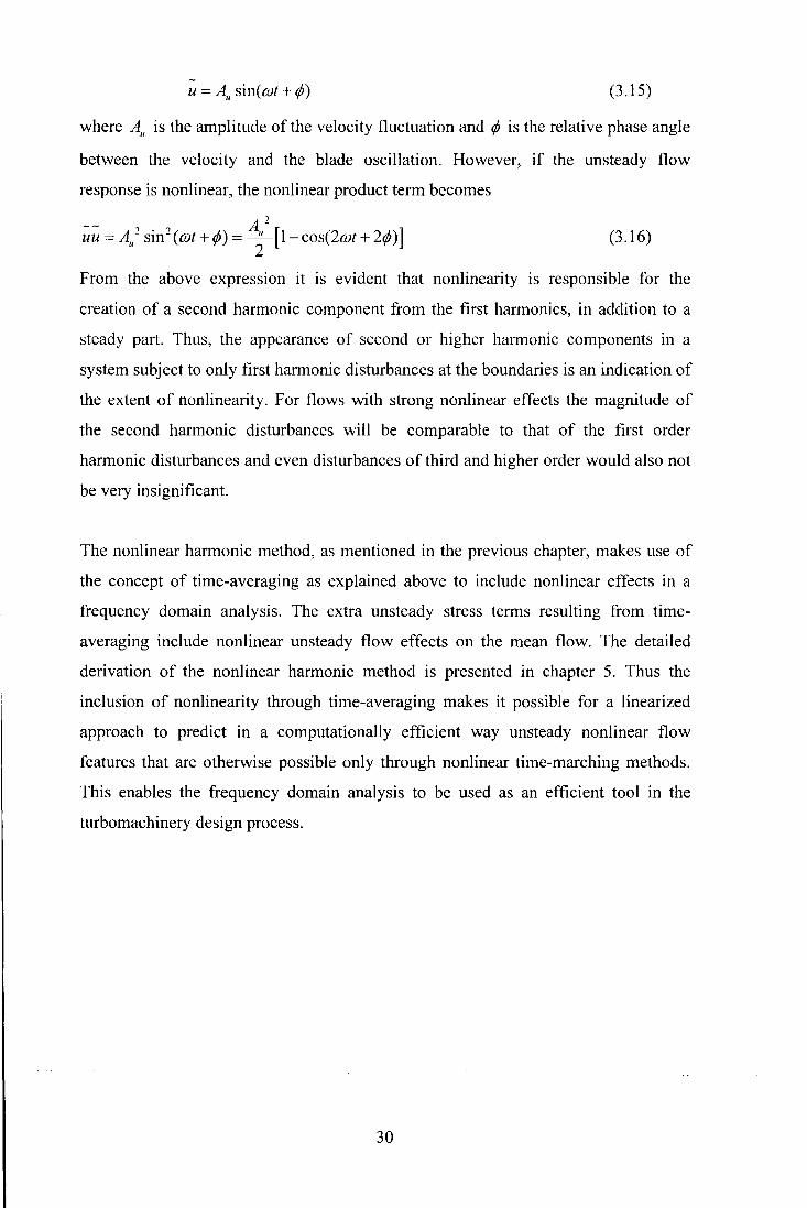
u = A11

sin(mt + ¢) (3.15)

where A" is the amplitude of the velocity fluctuation and ¢ is the relative phase angle

between the velocity and the blade oscillation. However, if the unsteady flow

response is nonlinear, the nonlinear product term becomes

-- A 2 uu = A11

2 sin2 (mt + ¢) = ~[l-cos(2mt + 2¢)] (3.16)

From the above expression it is evident that nonlinearity is responsible for the

creation of a second harmonic component from the first harmonics, in addition to a

steady part. Thus, the appearance of second or higher harmonic components in a

system subject to only first harmonic disturbances at the boundaries is an indication of

the extent of nonlinearity. For flows with strong nonlinear effects the magnitude of

the second harmonic disturbances will be comparable to that of the first order

harmonic disturbances and even disturbances of third and higher order would also not

be very insignificant.

The nonlinear harmonic method, as mentioned in the previous chapter, makes use of

the concept of time-averaging as explained above to include nonlinear effects in a

frequency domain analysis. The extra unsteady stress terms resulting from time­

averaging include nonlinear unsteady flow effects on the mean flow. The detailed

derivation of the nonlinear harmonic method is presented in chapter 5. Thus the

inclusion of nonlinearity through time-averaging makes it possible for a linearized

approach to predict in a computationally efficient way unsteady nonlinear flow

features that are otherwise possible only through nonlinear time-marching methods.

This enables the frequency domain analysis to be used as an efficient tool in the

turbomachinery design process.

30

Chapter 4

Linear Harmonic Method

4.1 Governing Equations

The basic laws of fluid dynamics are conservation laws that express the conservation

of mass, momentum and energy in a volume closed by a surface. Only with the

supplementary requirement of sufficient regularity of solution can these laws be

converted into partial differential equations. In case discontinuities such as shocks

occur, the solution of the differential equations is to be interpreted in a weak form, i.e.

as a solution of the integral form of the equations. In such cases, it is extremely

important that the conservation laws in their integral form are represented accurately.

The most natural method to accomplish this is to discretize the integral form of the

equations and not the differential form. The finite volume method is then the

appropriate choice for discretization.

The governing equations in the present case are three-dimensional Reynolds averaged

unsteady Navier-Stokes equations in cylindrical coordinates ( x, B, r) in an absolute

frame of reference. The integral form of the three-dimensional Navier-Stokes

equations over a moving finite volume !'!. V is

:t Jfiv UdV +eft[ (F- Fv )nx + (G- Gv )n8 + (H- H v )nr ]dA = JfivSdV

( 4.1)

where

p pu-pug pv- pvg pw- pwg

pu puu+ p- puug puv- puvg puw-puwg

U= pv ;F= r(puv- pvug) ;G= r(pvv+ p- pvvg) ;H= r(pvw- pvwg)

pw puw-pwug pvw-pwv g pww+p-pwwg

pe (pe+ p)u- peug (pe+ p)v- pevg (pe+ p)w- pew!?

0 0 0

r,

urr:r +vr,0 + wr,, -q,

31

and

0

0

S= 0

pv2 /r

0

r = 3_ Jl[2 ow _ _!_ av- au]- pw'w' rr 3 or r ae ox

[av I au] -, ,

r = r = Jl - +-- - pu v xe ex ox rae [

low av] -,, r =r = '' --+- -pvw

Br rB ,_ r o(} Or

[ax aw] -,,

rn = r,, = Jl or + ox - pw u

The inviscid fluxes in the three coordinate directions are represented by the flux

vectors F, G and H and the viscous fluxes are represented by the flux vectors

F;,, Gv and H v . The field vector U represents the vector of conservation variables.

In the above expression for the fluxes, u g, v g and wg are grid velocities, used to

accommodate the movement of the mesh due to the blade motion. The system of

equations is closed by an expression for pressure. For an ideal gas it is given by

p = (r -l)[pe-± p(u2

+v2 + w2)] (4.2)

The viscosity is Jl = JL1 + Jl,. The laminar viscosity JL1 is obtained from Sutherland's

law. For the present work, it is assumed that the laminar and turbulent viscosity

coefficients are frozen during linearization. The turbulent viscosity, Jl,, is obtained by

the standard Baldwin-Lomax algebraic mixing length model (Baldwin and Lomax,

1978). The coefficient of heat conductivity, k, is related to the viscosity through

Prandtl number.

4.2 Time Linearization

The governing equation can be linearized, provided the flow perturbations as well as

the effects of deterministic stresses are small enough compared to the steady flow.

The unsteady flow can be approximated as the sum of a mean or steady flow

component and a small disturbance unsteady component. The small perturbation

32

assumption is valid for flows where the unsteady perturbations are less than about

1 0% of the mean flow. Therefore, the unsteady flow can be represented as

.-.._

U(x,B,r,t) = U(x,B,r)+U'(x,B,r,t) (4.3)

However, many flows of interest are harmonic in time. Further, many flows that are

not harmonic are periodic in time. For the latter case, the unsteady perturbation flow

can be expressed as a Fourier series where the frequency OJ is 2tr/T. Since a linear

assumption has been made, the behaviour of each Fourier component can be analysed

individually, then summed together to form the total solution. Therefore, assuming

that unsteady flow can be divided into two parts, a steady flow and a small harmonic

perturbation part, for a single periodic disturbance, it can be represented as

~ -. - . U = U + Uelmt + U -e-Jmt (4.4)

Here U is the vector of complex amplitudes of perturbations in the conservation

variables given by

p

(pu)

U = (pv)

(pw)

(pe)

and U- is the complex conjugate of U .

(4.5)

The unsteady grid moving velocities ug, v g and wg are also assumed to change in a

harmonic form,

" (- iwt - -iwt) " (- iwt - -iwt) ug = Ug + Uge + Ug-e , vg = Vg + Vge + Vg-e ,

_,...,., - . - .

( /OJ{ -1{()()

wg = Wg + Wge +Wg-e (4.6)

For a rotor, Vg is the blade row rotating speed.

The computational grid is also assumed to undergo a small harmonic deformation

about its steady position, i.e.,

X=~+ (~eiwt + ~-e-iwt),B = {J + (Beiwt + B-e-ict1t ), r =; + (;eiwt +; -e-iM) (4.7)

Substituting the relationships (4.4) through (4.7) into the integral form of the

governing equation ( 4.1) and collecting the zeroth and first order terms, equation ( 4.1)

33

can be divided into two equations, i.e., the steady and the linearized unsteady

equations respectively. The steady equation is given by

cft[(F-Fv )dAx +(8-cv )dAo +(R -Hv )d71,.J = ffivsdv (4.8)

The linearized equation is

4JA[(F -Fv )dAx + (G-Gv )dAo +(H- Hv )dA,. +(F- Fv )dAx +

(G- Gv )dAo +(if- ii v )dA,.] = ffiv (siv + SdV)- im ffiv (uiv + uiv) (4.9)

All the variables in equations (4.8) and (4.9) are only space dependent and time does

not appear as they are cast in the frequency domain. The coefficients in the linearized

equation are obtained from the solution of the steady flow equation.

The perturbation fluxes are given by

---- - - ~ A A -

(pu)(u-ug)+(pu)(u-ug)+ p

F= r[(Pv)(~-~g)+(pv)(~-~g)J

(pw)(u- Ug) + (pw)(u- Ug)

[CPe)+ J;]~+[(pe)+ P]~-(Pe)~g -(pe)~g

(pu)(v- Vg) + (pu)(v- Vg)

G = r[ (Pv)(~ -~g)+ (pv)(~-~g) + J;] ----- - -

(pw)(v- Vg) + (pw)(v- Vg)

[CPe)+ J;]~+[(pe)+ P]~-(Pe)~g -(pe)~g

34

(pu)(w- Wg )+(pu)(w- Wg)

H = r[(;;)(~-~g)+(pv)(~-~g)J

-

0

0

S= 0

------ ~"""" -(pw)(w-wg)+(pw)(w-wg)+ p

[c0?)+ J;]~+[(pe)+ J;]~-(Pe)~g -(pe)~g

0

r XX

UT'xx + VT'xB + WT'xr + UT'xx +VI'_~+ WT'xr- qx

0

0

[ (Pv)~ + (pv)~Jjr 0

35

In the perturbation equation, the perturbation of viscosity is neglected by freezing the

viscosity to its steady value. Although the turbulence modelling could be linearized to

get the turbulent viscosity perturbation, this will increase the computation time and

make the code writing more complex. Under the Boussinesq approximation, the

primary role of turbulence is to provide enhanced diffusivities intended to mimic the

turbulent mixing. For moderate Mach numbers and moderate turbulent kinetic

energies, so long as there is no large separation, the interaction of the turbulence with

the mean flow is minor compared to the added diffusivity introduced by the eddy

viscosity. Holmes and Lorence (1997) have made blade flutter computations using a

linearized turbulence model and a normal turbulence model with frozen viscosity and

found that the results are nearly identical in both the cases for normal blade flutter

frequencies and the difference appears only in extremely low frequency cases

(reduced frequency of0.034).

4.3 Numerical Solution Method

Firstly, a steady flow solution is obtained by solving the steady Navier-Stokes

equation. The grid moving velocities are then prescribed according to the blade

vibrating mode shape. Then, for a given frequency and inter-blade phase angle, the

coefficients of the time-linearized equations are formed from the steady flow solution

and the time-linearized perturbation equations are solved. By linearization and

harmonic representation, solving a time-dependent unsteady problem in the time

domain is effectively transformed to solving two steady equations in the frequency

domain.

4.3.1 Pseudo Time Dependence and Numerical Discretization

In order to fully take advantage of the existing time-marching methods that are widely

used for steady flow calculations, a pseudo time variable ( t' ), as originally proposed

by Ni and Sisto (1976), is introduced to make the steady equation and the time­

linearized perturbation equation time-dependent, so equations (4.8) and (4.9) can be

rewritten as

!, fflvDdv +cft[cF -Fv )dAx +CG -ov )dAe +CH -ilv )dAr J = fft.sdv

( 4.1 0)

36

and

}___ ffi fJdv +A-r [(F -Fv )dAx +(G -Gv )dAe +(H -H v )dA,. +(F -Fv )dAx of' 1.\V 'tJ'A

+(G-Gv )dAe +(ii -iiv)dA,. J = fflv(sdv +SdV)-tw fff1.\v(udv +UdV)

( 4.11)

Now both the steady equation and the linear perturbation equation are hyperbolic in

nature and any well-developed time-marching scheme can be used to solve them.

Since only a steady state solution for steady flow equations and unsteady perturbation

equations is desired, any efficient acceleration technique like local time stepping and

multigrid can be used to speed up the convergence of the solution.

The spatial discretization for both Eq. (4.10) and Eq. (4.11) is made using a cell

centred finite volume scheme. For a hexahedral control volume, as shown in Fig. 4.1,

after semi-discretization, equations ( 4.1 0) and ( 4.11) can be written as

( 4.12)

and

(4.13)

where

-- - - - - - -Flux=(F+Fv)(~Axr +~Aor +~A,J+(G+Gv)(~Ax. +~Ao. +~A,.)+ .-....-...---

+(H +Hv)(~Ax, +~Ao, +~Ar,)

and

-- - - -- - --+(H +Hv)(~Ax, +~Ao, +~A,,)+(F+Fv)(~Ax, +~Ao, +~A,J - -- - -- -- --

+(G+Gv)(~Axo +~Ao0 +~A,.)+(H +Hv)(~Ax, +~Ao, +~Ar,)

-- - - - - ..........

Ax,, Ao, and A,, are steady projected areas and A,r, A or and A,, are unsteady

projected areas in the x direction of faces normal to the strearnwise, pitchwise and

..-... ......... -- ---- ......... -radial directions respectively. Similarly, Ax0 , Ao0 & Ar0 , A.,,, Ao, & Ar,. , Ax0 , Ao0 & A,8

- - -and Ax,, Ao, & A,, are steady and unsteady projected areas in the () and r directions

respectively. Fluxes in all three directions through faces in streamwise, pitchwise and

radial directions are summed up. For viscous fluxes, the first order spatial derivatives

37

are evaluated using the Gauss theorem. The cell centred finite volume scheme is a

spatial second order central difference scheme. In order to suppress numerical

oscillation, a second and fourth order adaptive smoothing (Jameson, 1981) is applied

in the streamwise, pitchwise and radial directions. The semi-discretized equations

(4.12) and (4.13) become

d...-..-... .,....,_,.....""" ....... ...-. _..-.. ..-.._ -(UdV) .. k = Rijk + dx +do+ dr- Dx- Do- Dr dt' lj

d-"' ~ ~ ~ ~----(UdV)lJ .. k = Rijk + dx +do+ dr- Dx- Do- Dr dt'

(4.14)

(4.15)

where dx,de and dr are second order steady smoothing terms and Dx,De and Dr

are the fourth order smoothing terms in x, B and r directions respectively. dx, de and

d r are the unsteady amplitudes of second order smoothing terms and Dx, De and Dr

are unsteady amplitudes of fourth order smoothing terms. For the steady flow

equations d, and Dx are given by

dx =c~~>cfJi+l,j,k -2Ui,j,k +Ui-l,J,k)t..V/M'

--- - (4) --- --- --- --- --- "I , Dx -EiJk (Ui+2,J,k -4U;+l,J,k +5U;,J,k -4Ui-IJ,k +U;-z,J,k)t..V M

where

and

(}<z> = Pi+l,J,k -2 Pi,J,k + Pi-i,J,k ijk

Pi+l,J,k + 2pi,J,k + Pi-l,J,k

( 4.16)

(4.17)

(4.18)

( 4.19)

(4.20)

where k< 2> is the second order smoothing coefficient with a typical value of 1/2 and

k< 4> is the fourth order smoothing coefficient with a typical value of 1/32. de,dr and

De, Dr can be given similarly.

For unsteady perturbation equation dx and Dx are given by

- - (2) - - - "I , dx - Eijk (Ui+l,j,k- 2Ui,j,k + ui-l.j.k) t..V f"..t (4.21)

38

(4.22)

The pressure sensor egl in the above expression ( 4.19) has not been linearized and

smoothing coefficients for the unsteady amplitudes are frozen at their steady value.

The unsteady fluctuations of the pressure sensor have been neglected here and this is

acceptable for and consistent with linear problems.

The pseudo time-marching for both the equations ( 4.14) and ( 4.15) is performed by

using the four stage Runge-Kutta scheme. The formulation for four stage Runge-Kutta

scheme from time step n to n+ 1 is

(4.23)

and

(4.24)

where k = 1 to 4, and for a four stage scheme the values of a are

4.3.2 Boundary Conditions

For a single blade passage domain as in the present case, there are four kinds of

boundary conditions, i.e. inlet, outlet, periodic and solid wall boundary conditions.

For steady flow calculation, the conventional boundary conditions are implemented.

A critical step in the implementation of boundary conditions is to separate the waves

into incoming and outgoing modes. The propagation properties in a one-dimensional

flow are expressed in a straightforward way by the characteristic variables. The form

of the missing information is defined by variables associated with the outgoing

characteristics. In a three-dimensional flow, for a subsonic inlet, four characteristics

are incoming and one is outgoing. At outlet, four characteristics are outgoing and one

is incoming. Therefore, at inlet, total pressure, total temperature and inlet flow angle

for subsonic flow or inlet Mach number for supersonic flow are prescribed, and the

static pressure at inlet is extrapolated from the interior domain. At outlet, the static

pressure is prescribed and other flow variables are extrapolated from the interior

domain. For periodic boundaries, a direct repeating condition is applied on both the

39

upper and lower boundaries. On the blade surface, zero flux is applied across the

boundaries for inviscid and viscous flow calculation. For viscous flow calculation,

either a no slip wall or slip wall boundary treatment can be used. For the no slip wall

boundary condition, the velocities on the blade surface are set to be zero and the wall

shear stress is evaluated from the local velocity gradients. The no slip wall boundary

condition requires a very fine mesh in the boundary layer region. For slip wall

condition, the wall shear stress for turbulent flows is approximated by a log law

formulation (Denton, 1990), as

where

CJ =

,... 1 " ,..,....._ ........... 2

Tw =-c1p2V2 2

2 ---- ;Re2 < 125 Re2

-0.001767 + O.O~ 77 + 0·25614 2 ; Re2 2125' ln(Re2) [ ln(Re2) J

(4.25)

(4.26)

(4.27)

The subscript 2 in the above expressions represents the mesh point one grid away

from the wall. The slip wall condition requires fewer mesh points near the wall than

the no slip wall condition and thereby saves computational time.

The boundary conditions for solving the time-linearized equations are different from

those for solving steady flow equations. For periodic boundaries, a phase-shifted

periodic condition is applied for solving the perturbation equation, i.e.

~u ~L . U =U ela (4.28)

where G" is the inter-blade phase angle and the superscript U refers to the upper

boundary and L refers to the lower boundary.

At inlet and outlet, the one-dimensional non-reflecting boundary conditions developed

by Giles (1990) and Saxer and Giles (1993) are implemented. The usual one­

dimensional approach is to assume perturbation travelling normal to the boundary in

40

the x direction. Hence the one-dimensional linearized Euler equations pre-multiplied

by the left eigenvector are written as

(4.29)

where ¢ = r-' fJ and A is the diagonal vector whose components represent the speed

of propagation (eigenvalues) of five characteristic waves, called the entropy, the two

vorticity and the upstream running and downstream running pressure waves. r-' is

the left eigenvector and ¢ is referred to as the vector of linearized characteristic

variables.

To implement the non-reflecting boundary conditions, firstly the transformation

between the amplitudes of five characteristic waves and amplitudes of pressure,

density and velocities are given by

and

1

c

p 0 u

v = 0

w

p 0

0

0

0

0

0

0

0

0

0 0 1 p

pc 0 0 u

0 pc 0 v

pc 0

-pc 0

0

0

1 w

1 p

0 0 "2

1 1 "2

2c 2c

0 0 1 1 t/J,

2pc

0 0 pc

0 1

0 0 pc

0 0 1

2 2

41

(4.30)

(4.31)

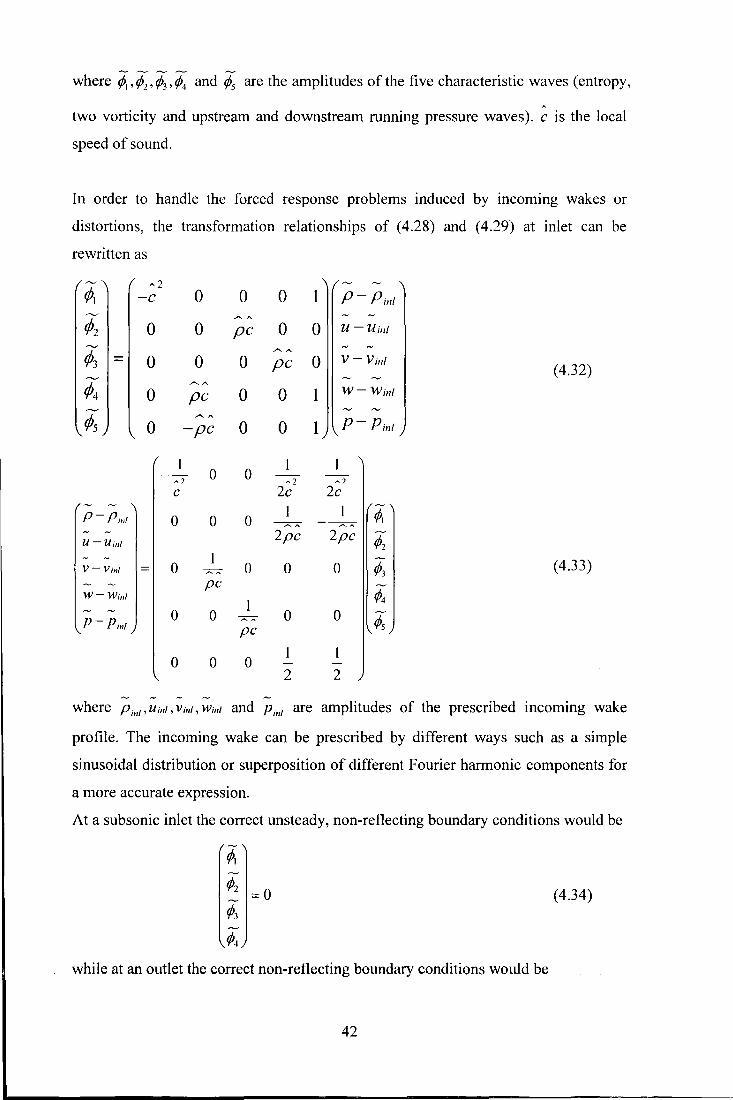
--------- --where rA, ¢2 ,¢3 , rA and ¢5 are the amplitudes of the five characteristic waves (entropy,

two vorticity and upstream and downstream running pressure waves). c is the local

speed of sound.

In order to handle the forced response problems induced by incoming wakes or

distortions, the transformation relationships of ( 4.28) and ( 4.29) at inlet can be

rewritten as

rA "2 -c 0 0 0 1 p- Pin/

(A 0 0 pc 0 0 U -Uinl

.......... .A" rA 0 0 0 pc 0 V- Vinl

(4.32)

¢4 0 pc 0 0 1 W-Winl

tPs 0 -pc 0 0 1 p- Pin/

~2 0 0

~2 ~2

c 2c 2c

p-pinl 0 0 0 I I ¢1 ~ ~~

U-Uinl 2pc 2pc ¢2

V-Vinl = 0 0 0 0 ¢3 (4.33) pc

¢4 W-Winl

p-pinl 0 0 0 0 rPs pc

0 0 0 I I

- -

2 2

where Pin!, Uini, Vini, Win! and Pin! are amplitudes of the prescribed incoming wake

profile. The incoming wake can be prescribed by different ways such as a simple

sinusoidal distribution or superposition of different Fourier harmonic components for

a more accurate expression.

At a subsonic inlet the correct unsteady, non-reflecting boundary conditions would be

(4.34)

while at an outlet the correct non-reflecting boundary conditions would be

42

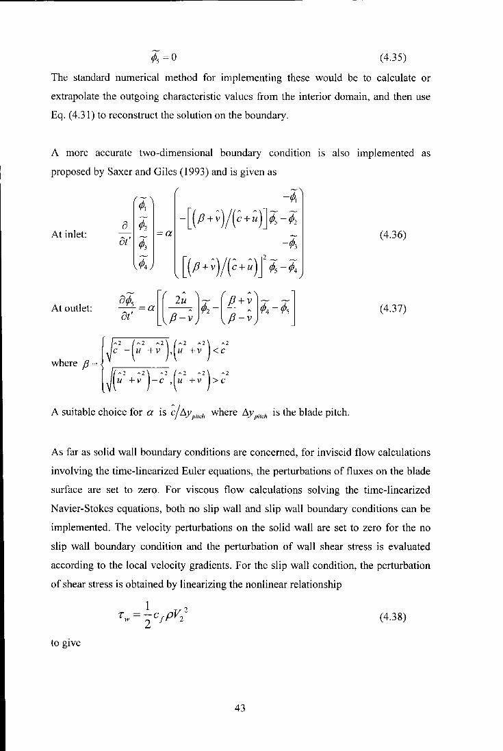
A. -0 'f/5 - (4.35)

The standard numerical method for implementing these would be to calculate or

extrapolate the outgoing characteristic values from the interior domain, and then use

Eq. (4.31) to reconstruct the solution on the boundary.

A more accurate two-dimensional boundary condition IS also implemented as

proposed by Saxer and Giles (1993) and is given as

-¢1

- [ ( fi + ~) / ( ~ + ~)] r/Js - r/J2

At inlet: =a (4.36)

At outlet: (4.37)

where f3 =

A suitable choice for a is ~ / b..y pilch where b..y pilch is the blade pitch.

As far as solid wall boundary conditions are concerned, for inviscid flow calculations

involving the time-linearized Euler equations, the perturbations of fluxes on the blade

surface are set to zero. For viscous flow calculations solving the time-linearized

Navier-Stokes equations, both no slip wall and slip wall boundary conditions can be

implemented. The velocity perturbations on the solid wall are set to zero for the no

slip wall boundary condition and the perturbation of wall shear stress is evaluated

according to the local velocity gradients. For the slip wall condition, the perturbation

of shear stress is obtained by linearizing the nonlinear relationship

(4.38)

to give

43

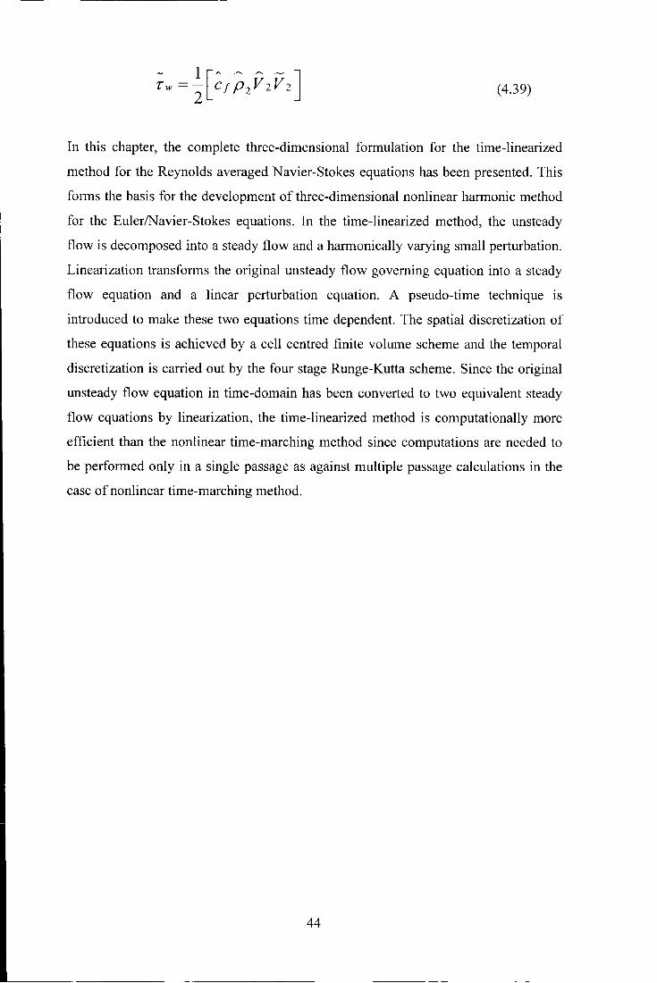
(4.39)

In this chapter, the complete three-dimensional formulation for the time-linearized

method for the Reynolds averaged Navier-Stokes equations has been presented. This

forms the basis for the development of three-dimensional nonlinear harmonic method

for the Euler/Navier-Stokes equations. In the time-linearized method, the unsteady

flow is decomposed into a steady flow and a harmonically varying small perturbation.

Linearization transforms the original unsteady flow governing equation into a steady

flow equation and a linear perturbation equation. A pseudo-time technique is

introduced to make these two equations time dependent. The spatial discretization of

these equations is achieved by a cell centred finite volume scheme and the temporal

discretization is carried out by the four stage Runge-Kutta scheme. Since the original

unsteady flow equation in time-domain has been converted to two equivalent steady

flow equations by linearization, the time-linearized method is computationally more

efficient than the nonlinear time-marching method since computations are needed to

be performed only in a single passage as against multiple passage calculations in the

case of nonlinear time-marching method.

44

Chapter 5

Nonlinear Harmonic Method

5.1 Time-Averaging and Incorporating Nonlinearity

The time-linearized approach results in solving two steady, single passage problems

instead of the original unsteady problem. The main feature of the time-linearized

approach is its high computational efficiency compared to the nonlinear time­

marching methods. However, this approach is restricted to linear problems due to the

linear assumption. Although the onset of flutter in turbomachinery is widely accepted

to be a linear phenomenon, the nonlinear effects with shock oscillations and viscous

flow separations can be potentially important. On the other hand, the forced response

of turbomachinery blades due to non-uniformity of unsteady flow fields like an

incoming wake, inlet distortion and potential interaction etc. is not necessarily a linear

phenomenon. Therefore, it is highly desirable to develop a numerical method that has

the high computational efficiency of time-linearized methods whilst including the

nonlinear effects like the nonlinear time-marching methods. The average passage

equation system formulated by Adamczyk showed that time-averaging the Navier

Stokes equations resulted in the inclusion of the effect of deterministic periodic

unsteadiness on the mean flow through stress terms similar to the Reynolds stresses.

Extra closure models are required to work out these deterministic stress terms similar

to turbulence modelling for Reynolds stress terms. Giles (1992) combined this

averaging approach with the linear unsteady flow modelling by including quadratic

source terms to account for the time-averaged effect. He (1996) proposed a nonlinear

harmonic methodology in which the extra stress terms in the time-averaged equations

are solved simultaneously with the harmonic perturbation equation using a strongly

coupled approach.

In the nonlinear harmonic method, a simple but significant change from the time­

linearized method is that a time-averaged flow field instead of a steady flow field is

used as the basis for the harmonic perturbations. The unsteady flow field is assumed

to be composed of two parts; a time-averaged flow plus an unsteady perturbation, e.g.,

U=U +U' (5.1)

45

where

p p' - (pu)' (pu)

U= r(pv) U'= r(pv)' - and (pw)' (pw) - (pe)' (pe)

(5.2)

and U is the vector of time-averaged conservative variables and U' is the vector of

perturbation variables. Similarly, the grid moving velocities are also divided into a

mean part plus a perturbation, i.e.

(5.3)

The computational grid can also be expressed by its steady position plus a small

perturbation, i.e.

x = x + x' , fJ = fJ + f)' , r == r + r' (5.4)

Substituting the expressions (5.1) through (5.4) into the original nonlinear integral

equation (4.1), and time-averaging it, the resultant time-averaged Navier-Stokes

equation can be given by

cfjA (F- Fv )d Ax+ (G- G;)d Ae + (H- H v )dAr+ (F'dA:) + (G'dA~) + (H'dA;)

-(F:dA:)-(G~~)-(H~dA;)= ffiv (SdV + S'dV') (5.5)

where

pu- pug

(pu- pug)u + p+(pu)'u'- (pug)'u'

F = r[(pu- pug)~+(pu)'v' -(pug)'v'] - ---

(pu- pug )w + (pu )' w'- (pug)' w'

(pu- pug )e + pu + p' u' + (pu)' e'- (pug)' e

46

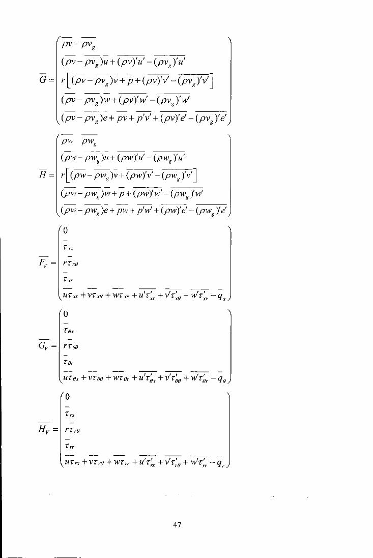
pv- pvg

(pv- pvg)u + (pv)'u'- (pvg)'u'

G = r[ (pv- pvg)~+ p + (pv)'v'- (pvg)'v']

(pv- pvg)w+ (pv)'w'- (pvg)'w'

(pv- pvg)e+ pv+ p'v' + (pv)'e'- (pvg)'e'

(pw- pwg)u + (pw)'u 1- (pwg )'u 1

H = r[(pw- pwg)~+(pw)'v' -(pwg)'v'] - ----

(pw- pwg)w+ p+ (pw)'w1- (pwg)'w'

(pw- pwg )e + pw + p 1W

1 + (pw)' e1- (pwg )' e'

0

Txx

Txr

I I f f f I U'[' xx + V'f xB + W'f xr + U 'f XX + V 'fx(} + W 'f xr - q X

0

I I f f f f UTox + VToo + WTor + U 'fox+ V Too+ W 'fer- qB

0

Trx

Trr

, , , , , , UT rx + VT rB + WT rr + U T,-x + V TrB + W Trr - q r

47

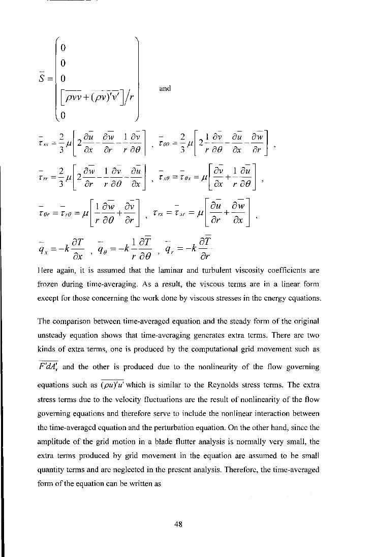
0

0

S= 0

[pv~ + (pv)'v']/r and

0

[ - -] - - av 1 au , TxB =Tax= f.1 ax+-; a(} ,

Here again, it is assumed that the laminar and turbulent viscosity coefficients are

frozen during time-averaging. As a result, the viscous terms are in a linear form

except for those concerning the work done by viscous stresses in the energy equations.

The comparison between time-averaged equation and the steady form of the original

unsteady equation shows that time-averaging generates extra terms. There are two

kinds of extra terms, one is produced by the computational grid movement such as

F'dA_: and the other is produced due to the nonlinearity of the flow governing

equations such as (pu )' u' which is similar to the Reynolds stress terms. The extra

stress terms due to the velocity fluctuations are the result of nonlinearity of the flow

governing equations and therefore serve to include the nonlinear interaction between

the time-averaged equation and the perturbation equation. On the other hand, since the

amplitude of the grid motion in a blade flutter analysis is normally very small, the

extra terms produced by grid movement in the equation are assumed to be small

quantity terms and are neglected in the present analysis. Therefore, the time-averaged

form of the equation can be written as

48

ct.fA[(F-F;/)dAx +(G-Gv)dAe +(H -Hv)dAr] = ffivSdV

(5.6)

The extra terms appear in the time-averaged momentum and energy equations. To

solve the above time-averaged equation, extra relationships are required to make the

equation closed. Nonconservative variables can be worked out from time-averaged

conservative variables, for example,

- - -;-u = (pu-p' u') p (5.7)

5.2 First Harmonic Perturbation Equation

Substituting the expressions (5.1), (5.3) and (5.4) into the original governing equation

and then subtracting the time-averaged equation, the unsteady perturbation equation is

given by

:t ffiv(UdV' +UliV)+cffA(F' -Fv')dAY +(G' -G~)dA8 +(H' -H~)dAr

+(F- Fv )dA_: +(G- Gv )dA~ +(H -H v )dA;] = fJL/SdV' +S'dV)

where

(pu )'-(pug)'

(pu- pug )u' + [ (pu)'- (pug r]~+ p'- (pu)' u' +(pug)' u

F' = r[ (pu- pug)v' + [ (pu)'- (pug)']~- (pu)'v' +(pug }v'] (pu- pug )w' + [ (pu )'-(pug)' J w- (pu )' w' +(pug)' w'

(5.8)

(pe+ p)u' + [ (pe)' + p']~- (pe)u~- (pe)'ug- p'u'- (pe)'u' + (pe)'u~

(pv)' -(pvg)'

(pv- pvg)u' +[ (pv)'- (pvg)']~- (pv)'u' + (pvg)'u'

G' = r[(pv- pvg)v' +[(pv)' -(pvg)']~+ p' -(pv)'v' +(pvg)'v']

(pv- pvg)w' + [ (pv)'- (pvg)'] w- (pv)'w' + (pvg)'w'

(pe+ p)v' +[(pe)' + p']~-(pe)v~ -(pe)'vg- p'v' -(pe)'v' +(pe)'v~

49

(pw) 1 -(pwg)1

(pw- pwg)u 1 + [ (pw) 1- (pwg)1]~ -(pw)'u 1 + (pwg)'u 1

H 1 = r [ (pw- pwg)V1 + [ (pw)'- (pwg)'];- (pw) 1V1 + (pwg)1

V1

]

(pw- pwg)W1 + [ (pw)'- (pwg)'] w+ p 1- (pw) 1W1 + (pwg)'w 1

and

(pe + p)w1 +[(pe)1 + p1]w-(pe)w~ -(pe)'wg- p 1W1 -(pe) 1W1 + (pe)'w~

0 I

rxx

F,:= r<o - -- --

1 I I I I I I I I I I I I

ur_U + vr x(} + -wfxr + U r_'(X + V r x(} + W rxr - q X - U r_'(X - V rx(} - W rXr

0

- ------1 I I I I I I I I I I I I

ur(}x + vr(}(} + wr(}r + u r(}x + v r(}(} + w r(}r- q(}- u r(}x- v r(}(}- w r(}r

0

- ------1 I I I I I I I I I I I I

ur,-x + vrr(} + -wrrr + u rrx + v rr(} + w rrr- qr- u rrx- v rr(}- w rrr

0

0

S'= 0

[pw' +(pv)'~-(pv)'v']/r 0

r' = 2 //[2 au'- aw' _ _!_ av'] r' = ~ //[2_!_ av'- au'- aw'] XX 3 r 0x ar r ae ' (}(} 3 r r ae 0x ar

50

, _-kaT' , = -k _!_ ar' , _-kaT' qx - ax ' q(} r ae ' q,. - ar

The complete form of the unsteady perturbation equation is not readily solvable if a

frequency domain approach is to be used. It is assumed that the unsteady perturbation

is dominated by first order terms. Retaining only the first order terms, the resultant

first order form of the fluxes can be rewritten as

(pu )'-(pug)'

(pu- pug )u' + [ (pu )'-(pug)' J~ + p'

F' = r [ (pu- pug)v' + [ (pu)'- (pug)']~]

(pu- pug)w' +[ (pu)' -(pug)'] w

(pe+ p)u' +[(pe)' + p']~-(pe)u~ -(pe)'ug

(pv)' -(pvg)'

(pv- pvg)u' + [ (pv)'- (pvg)'];;

G' = r[(pv- pvg)v' +[(pv)' -(pvg)']~+ p'] (pv- pvg)w' +[ (pv)' -(pvg)']w

(pe+ p)v' +[(pe)' + p']~-(pe)v~ -(pe)'vg

(pw)'- (pwg )'

(pw- pwg)u' +[ (pw)'- (pwg)']~

H' = r[ (pw- pwg)v' +[ (pw)'- (pwg)']~J

(pw- pwg)w' +[ (pw)'- (pwg)']w+ p'

(pe+ p)w' +[ (pe)' + p'] w- (pe)w~- (pe)'wg

51

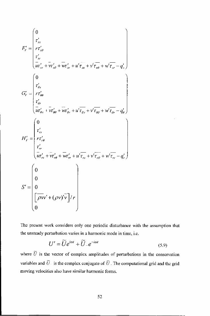
0 I

'xx

F;; = rr_:e

I I I I I I I

ur xr + Wxe + wrxr + U r_u: + V 'xo + W rxr - qx

0 I

'ox

G~ = rr~0

-I I I I I I I

Uf' Ox + W BO + Wf Or + U f' Ox + V f' 00 + W f' Or - qg

0

H~=

0

0

S1 = 0

[pvv 1 +(pv)'~]! r 0

The present work considers only one periodic disturbance with the assumption that

the unsteady perturbation varies in a harmonic mode in time, i.e.

U' = U eicvt + fJ _e-iwt (5.9)

where fJ is the vector of complex amplitudes of perturbations in the conservation

variables and U- is the complex conjugate of U . The computational grid and the grid

moving velocities also have similar harmonic forms.

52

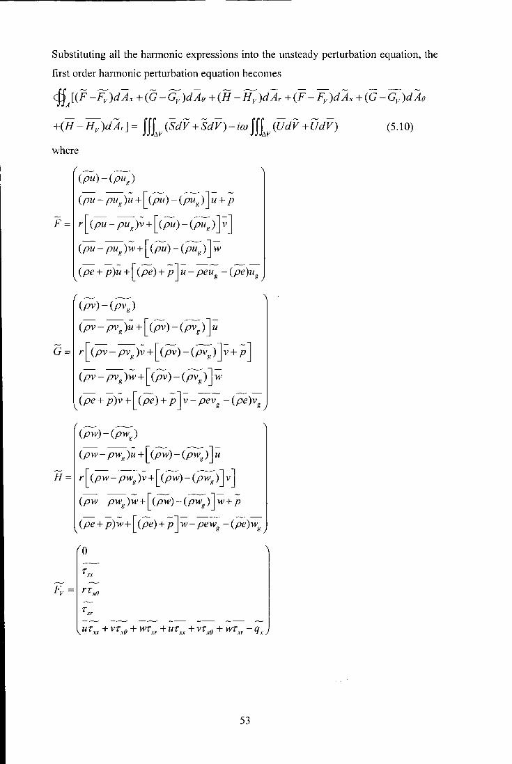
Substituting all the harmonic expressions into the unsteady perturbation equation, the

first order harmonic perturbation equation becomes

cff)CF -Fv )dAx + (G -Gv )dAe + (H- Hv )dAr+ (F- F;, )dAx +(G- Gv )dAe

+(H-Hv)dAr]= fflv(SdV+SdV)-im fflv(UdV+UdV) (5.10)

where

(pu)-(pu~)

(pu- pug)~+ [ (pu)- c-;;z;:) J ~ + p f' = r [ (pu -pug)~+ [ (pu)- c-;;z;:) J ~ J

(pu- pug);+[ (pu)- (-;;;;:) J w

(pe + p)~ +[ (pe) + 'P]~- peug- (pe)ug

(pv)- (pvg)

(pv- pvg)~ +[ (pv)- cty;;) ]~

G = r[ (pv- pvg)~+[ (pv) -(~) ]~+ 'P] (pv- pvg)~'+[ (pv)- (ty;;) J w

(pe + p)~ +[ (pe) + 'P]~- pevg- (pe)vg

(pw)-(pwg)

(pw- pwg)~+[(pw)-(j;~~)]~

H = r[ (pw- pwg)~+[ (pw)-(p;;)J~J

(pw- pwg);+[(pw)-(p;;)J~+ p (pe+ p)~+[ (pe)+ p];- pewg -(pe)wg

0

53

-

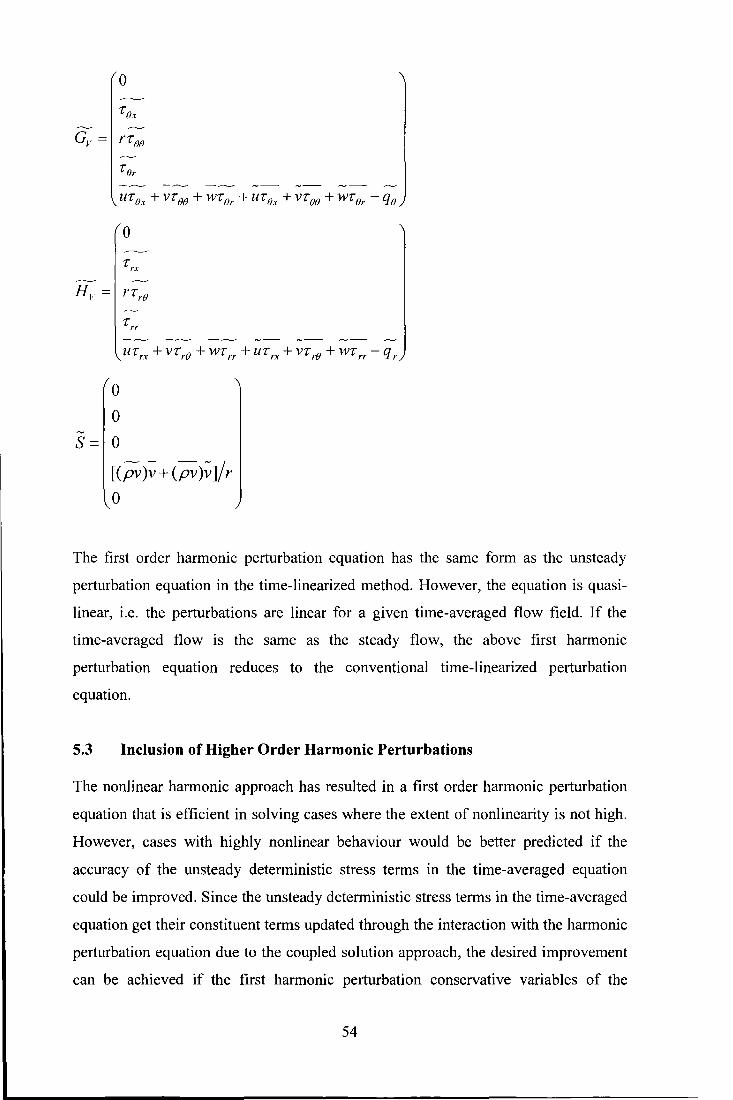
0

0

0

0

T,.x

T,.,.

S= 0

[(pv)~ + (pv)~ J/r

0

The first order harmonic perturbation equation has the same form as the unsteady

perturbation equation in the time-linearized method. However, the equation is quasi­

linear, i.e. the perturbations are linear for a given time-averaged flow field. If the

time-averaged flow is the same as the steady flow, the above first harmonic

perturbation equation reduces to the conventional time-linearized perturbation

equation.

5.3 Inclusion of Higher Order Harmonic Perturbations

The nonlinear harmonic approach has resulted in a first order harmonic perturbation

equation that is efficient in solving cases where the extent of nonlinearity is not high.

However, cases with highly nonlinear behaviour would be better predicted if the

accuracy of the unsteady deterministic stress terms in the time-averaged equation

could be improved. Since the unsteady deterministic stress terms in the time-averaged

equation get their constituent terms updated through the interaction with the harmonic

perturbation equation due to the coupled solution approach, the desired improvement

can be achieved if the first harmonic perturbation conservative variables of the

54

harmonic perturbation equation are made more accurate· by including higher order

harmonic perturbations through a cross coupling of perturbation terms in the

harmonic perturbation equation itself. This higher order cross coupling in turn

improves the first harmonic perturbation conservative variables that form the unsteady

stress terms in the time-averaged equation. This is achieved by a harmonic balance

technique that has its origins in the field of structural dynamics.

5.3.1 Harmonic Balance Method

For simplicity, the details are first expressed in a formulation of one dimension and

later extended to three dimensions.

Considering the one dimensional momentum equation,

a a a -(pu)+-(pu·u+ p)--(r) = 0 at ax ax (5.11)

and assuming that the flow is composed of a time-averaged part and a harmonic

perturbation part, the flow variables can be expressed as -

u =u+u' (5.12)

and

pu = pu + (pu )' (5.13)

The pressure is also similarly decomposed. Substituting (5.12) and (5.13) into the one

dimensional momentum equation ( 5.11) and time averaging it, we get the time­

averaged equation as

a-- -a--(pu·u+(pu)'u' + p)--(r) = 0 ax ax (5.14)

The above time-averaged equation is the same as in nonlinear harmonic approach.

Since the unsteadiness in the flow is assumed to be harmonic in time, the perturbation

variable u' in equation (5.12) can be expressed as a complex Fourier series to give,

N f '"'(- in(tJf - -inmt) - -imt - i(tJf - -i2mt - i2mt u = ~ Une +u-ne =U-Ie +u,e +u-2e +u2e + .....

n=l

(5.15)

- -where n is the order of harmonics, u_, is the complex conjugate of u, and N is the

total number of perturbations to be included. Since conservation variables are real

quantities, we only need to have Fourier coefficients for non-negative n. Similarly,

(pu )' in Eq. ( 5.13) can be expressed as

55

-------------------------------------------------------·----··

N

(pu)' = L ((puteinwt +(pu)_ne-inwt) = (pu)_l e-iwt +(pu)l eiwt + .... n=l

(5.16)

Substituting (5.12), (5.13), (5.15) and (5.16) into the momentum equation (5.11) and

collecting only the first order harmonic terms, we get the first order harmonic

perturbation equation as

~ a -- -~ ~- - ~ ~-im(pu)1 +ax [(pu)UI + u(pu)1 + (pu) 2 U-1 + U2(pu)_ 1 + (pu) 3 U-2

-~ a~ a~ +u3(pu)_2 + .... ]+-(p1)--(r1) = 0 (5.17)

ax ax

The order of harmonics of each term in (5.17) is one. In the case of terms involving

the product of fluctuations, the sum of the harmonics should be equal to one

(e.g., (pu )3

eiJrvt • u_2e -ilwt ). In this way, the harmonic balance is achieved for the entire

equation. Therefore, the general form (e.g. for OJ11

) of harmonic perturbation equation

can be expressed as

~ a { - - - ~ [ ~ - J} a ~ a -im(pu)11+- (pu)u

11+u(pu)

11+ L (pu)iul +-(p

11)--(r

11)= 0

OX i+ j=n OX OX

(5.18)

where i,j = ±1,2,3, ........... and n could be of any order of harmonics subject to the

condition that i + j = n. The zeroth harmonic, n = 0, corresponds to the mean flow. In

principle, the summation of harmonics i and j can be taken over all integer values of

n. In practice, however, they are truncated to a finite number of harmonics. The

equation (5.18) has a cross coupling term L (pu)i~J that has resulted from the i+j=ll

inclusion of higher order harmonics, which differentiates this equation from the one

obtained through the nonlinear harmonic formulation. Also, the deterministic stress

term in (5.14) can now be expressed as (pu)'u' = t[ (pu)11 ~-~~ + (pu)_~~~~~J.It is clear

from the above that with the inclusion of higher order harmonics the accuracy of

deterministic stress terms will improve as the cross coupling term in the harmonic

perturbation equation helps to refine the fundamental harmonic terms in a coupled

solution approach. If no higher order harmonics are considered, the first order

56

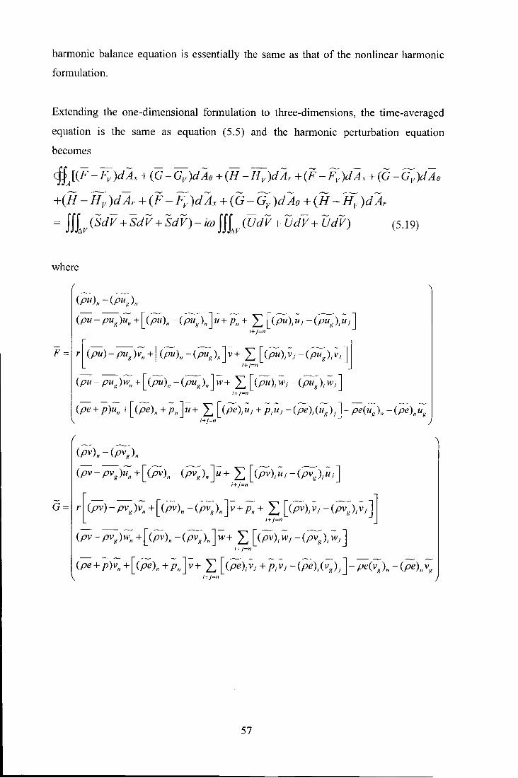
harmonic balance equation is essentially the same as that of the nonlinear harmonic

formulation.

Extending the one-dimensional formulation to three-dimensions, the time-averaged

equation is the same as equation (5.5) and the harmonic perturbation equation

becomes

c#)CF -Fv )dAx +(G-Gv)dAe +(H -H v)dAr +(F -Fv)dAx +(G -Gv)dAe - --- - ---- -.....-- -...... .- - ............. - ---- --

+(H -Hv)dAr +(F-Fv)dAx +(G-Gv)dAo +(H -Hv)dAr

= Jfiv (SdV + SdV + SdV)- im Jfiv (UdV + UdV + UdVJ (5.19)

where

(pu), -(pux),

(pu- pux)un +[(pu), -(p;:-).,]~+ p, +I [(pu)i~J -(p;:-)i~J J i+j=n

F ~ +pu)- pu,)V;> [ (pu),- (PU,), JV+,.~~J (pu),;; 1 -({;U;), ;;i]]

(pu- pux)w, +[(pu), -(p;:-),];+ I [(pu)i ;,J -(p;:-)i ;,J J i+j=n

(pe + p)u, + [ (pe), + p, ]~ + I [ (pe)i~J + pi~J- (peMug)J J- pe(ug)n- (pe),ug i+j=n

(pv)n- (pvg)n

(pv- pvg)u11 +[(pv)~~-(~),]~+ I [Cpv)i~J -(~)i~J] i+j=n

G ~ r[cpv)- pv,)v, +[(pv), -(pv,),}+ p, + ,~J (pv),VJ-(Pv,),Vi]]

(pv- pvg)wn +[(pv), -(pv~\ ];+I [Cpv)i ;,J -(p~\ ;,J] i+j=n

(pe + p )~ + [ (pe) II + p n J ~ + L [ (pe) j ~ j + p j ~j - (pe M v g); J - pe( v X) n - (pe) II v g i+j=n

57

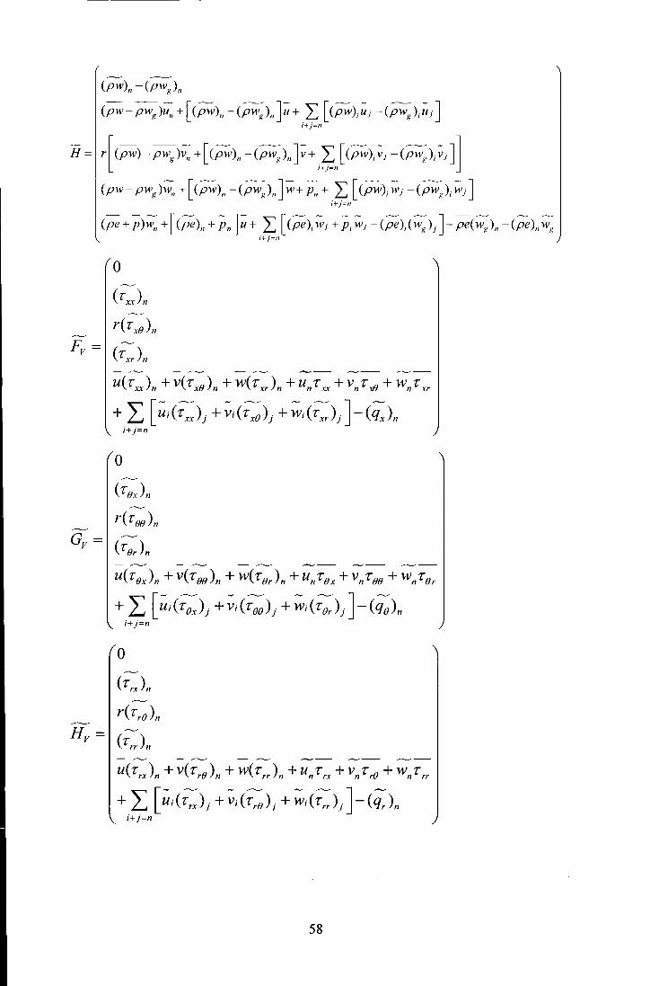
(pw)" -(pw8 )"

(pw-pwg)u11 +[(pw)11 -(~)11 ]~+ I [(pw);;J-(~);;i] i+j=n

H ~ +pw)- pw, )i\, + [ (pw )" - (P,V,\ J V + ,~J<pw ), V, - <P.: ), V 1]] (pw- pw8 )w11 +[(pw)" -(~)"];+ p" +I [(pw); ~'i -(~); ~'J J

i+j=n

(pe + p)w" + [ (pe) 11 + Pn ]~ + I [ (pe); ~'J + P; ~'J -(pe);(w,,)i J- pe(1-vx)" -(pe)11 wg

0

( r."-.Jn

r(rxot

Fv = ( ) r_w 11

i+j=n

U(TX-. ..)11 + V(TxB)n + W(rxJn + U 11 'f xx + V11 'f).{)+ W 11 'f_w

+I [~;(rx.-JJ +~;(rxB)J +;;(rxJJ]-(qJn i+j=n

0

(rBJ11

r(roo)n

Gv = ( ) TBr n

u(ro . ..Jn + v( TBB)11 + w(rBr)n + Un TBx + Vn TBB + Wn TBr

+I [~;(ro_..JJ +~;(roB)J +;;(ror)J ]-Cqo)n i+j=11

0

(rn;)11

r(rrB )n

Hv = ( ) rrr n

+I [~;(rrx)J+~;(rrB)J+;;(rrr)JJ-(qr)11 i+j=n

58

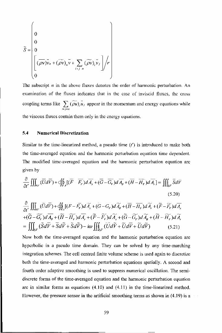
0

0

S= 0

[(pv)~, +(pv),~+ ;~, (pv); ~j ]f 0

The subscript n in the above fluxes denotes the order of harmonic perturbation. An

examination of the fluxes indicates that in the case of inviscid fluxes, the cross

coupling terms like L (pu);~J appear in the momentum and energy equations while i+}=ll

the viscous fluxes contain them only in the energy equations.

5.4 Numerical Discretization

Similar to the time-linearized method, a pseudo time (t') is introduced to make both

the time-averaged equation and the harmonic perturbation equation time dependent.

The modified time-averaged equation and the harmonic perturbation equation are

given by

:, fflv(UdV)+cfjA[(F-Fv)dA, +(G-Gv)dA0 +(H -Hv)dA,] = fflvSdV

(5.20)

:, fflv (UdV) + cffA [(F- Fv )d A,+ (G- Gv )d A0 + (H- Hv )d A,+ (F- Fy. )d A,

-~-- -~- -~~ -~.........__.. -----~

+(G-Gv )dA0 +(H -Hv )dA, +(F -Fv )dAx +(G-Gv )dA8 +(H -Hv )dA,

= Jfiv (SdV + SdV + SdV)- iw Jfiv (UdV + UdV + UdV) (5.21)

Now both the time-averaged equation and the harmonic perturbation equation are

hyperbolic in a pseudo time domain. They can be solved by any time-marching

integration schemes. The cell centred finite volume scheme is used again to discretize

both the time-averaged and harmonic perturbation equations spatially. A second and

fourth order adaptive smoothing is used to suppress numerical oscillation. The semi­

discrete forms of the time-averaged equation and the harmonic perturbation equation

are in similar forms as equations ( 4.1 0) and ( 4.11) in the time-linearized method.

However, the pressure sensor in the artificial smoothing terms as shown in (4.19) is a

59

nonlinear term and its nonlinearity cannot be ignored in cases with strong nonlinear

effects. Therefore, it is desirable to linearize the pressure sensor. Since an accurate

way to linearize the pressure sensor is not easy to achieve, an approximate approach is

used to partially linearize the pressure sensor (He and Ning, 1998). The modified

form of the pressure sensor is given by

P . I .k -2p. 'k +p. I .k Bk = 1- ,], 1,], I+,],

I)

P;-l,j,k + 2 Pu,k + P;+IJ,k

pi+l,j,k -2 P;,j,k + Pi-l,j,k + 0. 5 =-------==----=----1

P . I . k + 2p . . k + P· I . k I+ ,) , I,), I+ ,) ,

(5.22)

The modified pressure sensor is proportional to the local unsteadiness and the time­

averaged effects of the nonlinear behaviour of pressure sensor can be included.

5.5 Coupling Between Time-Averaged Flow and Unsteady Perturbation

In order to close the time-averaged equation, extra relationships are needed. For a

periodically unsteady flow, these terms can be directly evaluated in terms of the

unsteady perturbations. For example, u' and v' are two unsteady quantities changing

in the harmonic form, i.e.

N 1 """' (- incot + - -incot)

U = ~ Une U-ne (5.23) n=I

and

N

v' =I c ~neincot + ~-ne-incot) (5.24)

n=I

Time-averaging the product u'v' gives the deterministic stress

(5.25)

By using the relationship (5.25), the extra terms in the time-averaged equation (5.20)

can be worked out if the unsteady perturbations are already known. The unsteady

perturbations are obtained by solving the harmonic perturbation equation whose

coefficients are formed from the solution of the time-averaged equation. Therefore,

the time-averaged equation and the harmonic perturbation equation interact with each

other. Because of this interaction, these two equations cannot be solved separately and

a coupling procedure has to be used. The time-averaged equation and the harmonic

60

perturbation equation have to be solved simultaneously. A strong coupling technique

proposed by He (1994) is used to time-march the time-averaged flow field and the

unsteady perturbations. This strong coupling procedure is illustrated in Fig. 5.1. This

strong coupling procedure provides high stability that is particularly useful when the

interaction between time-averaged flow and unsteady perturbations becomes strong.

For the pseudo-time time integration of both the time-averaged equation and the

harmonic perturbation equation, the four-stage Runge-Kutta time-marching scheme is

used. The boundary conditions are the same as those applied in the time-linearized

method and the only difference is that the steady flow variables in the boundary

conditions are replaced by time-averaged variables.

In this chapter, the complete three-dimensional formulation for the nonlinear

harmonic method for the Reynolds averaged Navier-Stokes equations is presented. In

addition, the inclusion of higher order harmonics to the basic nonlinear harmonic

method through harmonic balancing has also been presented for the three-dimensional

Reynolds-averaged Navier-Stokes equations. When compared to the time-linearized

method there are some distinctive features of the nonlinear harmonic method that

needs to be mentioned. In this method, the unsteady flow is divided into a time­

averaged part and a perturbation part and the time-averaging brings in extra stress

terms that account for the nonlinear behaviour. Then the time-averaged equation and

the harmonic perturbation equation are solved using a strong coupling method that

facilitates the updating of the unsteady stress terms. Also, the pressure sensor in the

smoothing terms is suitably linearized to include the time-averaged effects of the

nonlinear behaviour of the pressure sensor. Though the coupling procedure solves

both the time-averaged and the first order perturbation equations simultaneously, the

scheme is computationally more efficient compared to the nonlinear time-marching

method while including nonlinear effects. The inclusion of higher order harmonics

through cross coupling raises the computational effort compared to the solution of the

first order perturbation equation alone but the computational efficiency is still

considerably higher than the nonlinear time-marching method.

61

Chapter 6

Two-Dimensional Results and Discussion

A three-dimensional Navier-Stokes solver incorporating the time-linearized method

and nonlinear harmonic method has been developed for unsteady flows in

turbomachinery. This has to be validated against a series of test cases to demonstrate

the efficiency of the frequency domain approach. However, since validation of three

dimensional unsteady flows is particularly difficult due to lack of experimental data,

the basic methods are first validated by computing two-dimensional inviscid and

viscous test cases. The validation consists of linear test cases for blade flutter and

forced response problems and nonlinear test cases for transonic flow in a diverging

channel and transonic flow through an axial flow fan. Depending on the test case

considered, the calculated results will be compared with results from any one of these

three sources; numerical results produced by well-developed linear theories, nonlinear

time-marching method and experimental data.

6.1 Oscillating Flat Plate Cascade

The basic time-linearized method is validated by computing the unsteady inviscid

flows around an oscillating flat plate cascade. The specifications of this cascade is

Chord =0.1 m

Solidity (Chord/Pitch) = 1.0

Stagger angle = 45°

The flow has a Mach number of0.7 at zero incidence.

The unsteady flows are introduced by the blade oscillation in a bending mode normal

to the chord with an amplitude equivalent to 1% of the chord for four inter-blade

phase angles of 90°, 180°, -90° and 0°. The unsteady flows are also computed for

blade oscillation in torsion mode around the blade leading edge with 1 degree

amplitude for the four above-mentioned inter-blade phase angles. The calculations for

both the bending and torsion modes were carried out for a reduced frequency, based

on blade chord and flow inlet velocity, of 1.0.

The unsteady pressure jump coefficient is defined by

62

-f'..p

c p = --~-----=---,~ 2=--- ,......._ ...... 2

(p)' -(p)" (6.1)

0.5 P;,1UreJA111 0.5p;,1UreJA111

where Am is the non-dimensionalized amplitude of blade motion, and the superscript

"u" represents the upper surface of a reference blade and "1" refers to the blade lower

surface.

Fig. 6.1 through Fig. 6.4 show the real (in-phase) and imaginary (out-of-phase) parts

of the calculated unsteady pressure JUmp coefficient plotted against

nondimensionalised blade chord. The calculated values are compared to those

generated by the linear analytical solver LINSUB. The programme LINSUB was

developed by Whitehead (1987) based on a semi-analytical linear method and it can

handle several kinds of turbomachinery unsteady flows in a flat plate cascade induced

by blade oscillation, incoming wakes and inlet or outlet pressure disturbances. The

comparison between the calculated values obtained by the present solver and those

obtained by LINSUB is good.

Figs. 6.5 and 6.6 show the real and imaginary parts of the calculated force and

moment coefficients at different inter-blade phase angles for bending and torsion

modes of oscillation. Also shown are the corresponding values obtained from

LINSUB. For the bending mode, the imaginary parts of force and moment

coefficients agree well with the values from LINSUB while the real parts show some

discrepancy for the phase 180°. On the other hand, in the case of torsion, the

imaginary parts of force and moment coefficients show a higher value for 180°. The

solution from LINSUB is based upon the distribution of a vorticity sheet along the flat

plate cascade that satisfies the inviscid boundary condition that there is no relative

flow normal to the flat plate. The resulting integral equation is solved computationally

in LINSUB, but the solution can be obtained so accurately that for test purposes it

may be considered to be an exact analytic solution. The present calculation, on the

other hand, uses unsteady boundary conditions in different ways. For unsteadiness

due to blade vibration, the grid nodes on the blade move with the blade, and this

produces extra flux terms due to grid movement that is taken account of in the

formulation. In the case of wake/blade row interaction, the velocity profile of the

wake coming into the blade row is specified. In the case of unsteadiness due to static

63

pressure fluctuations at the exit, a sinusoidal variation is assumed. In all these cases,

the boundary conditions are formulated in a non-reflecting manner, to ensure that

outgoing pressure and vorticity waves do not produce artificial reflections at the inlet

and outlet boundaries. This difference in the treatment between the analytical method

and the present numerical method could be the reason for the discrepancies observed.

A reasonably good comparison for the force and moment coefficients is an indication

that any computation of aerodynamic damping based on these parameters is reliable.

This information is useful to the turbomachine designer for judging the aeroelastic

behaviour of a specific cascade.

6.2 High Frequency Incoming Wakes

In order to assess the ability of the present time-linearized method to handle forced

response problems in turbomachinery, the unsteady inviscid flows around a flat plate

cascade induced by high frequency unsteady incoming wakes have been calculated.

In this case, the geometrical parameters ofthe cascade are:

Chord

Solidity

=O.lm

= 2.0

Stagger angle = 30°

The inlet flow has a Mach number of 0.7 and flow angle of 30°. The unsteady

incoming wake has a pitch that is 90% of the blade pitch and the corresponding

reduced frequency, based on axial velocity and axial chord, is 13.96 for an inter-blade

phase angle of -400°, corresponding to an incident wake to blade count ratio of I 0/9.

The wake in this calculation is prescribed by assuming a uniform static pressure,

uniform total enthalpy and a simple sinusoidal form of velocity defect across the wake,

so the unsteady perturbation amplitude of the incoming wake can be given by

p=O.O

A2 A2 u=A

111 U;n/ + Vinl cos(Pwake)

A2 A2 V -A - m Uinl + Vinl sin(Pwake)

where P ... ake is the angle of the incoming wake and has a value of -30° in this

calculation. Am is the amplitude of the wake velocity defect and has a value of 1 %.

64

The amplitude of the wake density, Pin!, can be worked out by linearizing the

following nonlinear relationship

P- = _!__ Pin/

in/ 1 ( 1 J r- · 2 2 c pr;nl - 2 uinl +villi

(6.2)

where r*int is the inlet total temperature and is constant in the wake frame. For the

wake in this calculation, Pint is given by

where cp is the gas constant and r is the ratio of specific heats.

The unsteady pressure coefficient jump in this case is defined by

-11p c" =~A _

pUre!Uref

(6.3)

(6.4)

where Uref is the velocity perturbation which would be induced at the leading edge of

the blade by inlet wakes, if the cascade were removed.

In order to resolve the high frequency (short wave length) unsteadiness, a fine mesh

with a size of 400 x 50 is used in this calculation. Fig. 6. 7 provides the comparison of

unsteady pressure coefficient jump between values calculated by the present code and

those obtained by LINSUB. For an unsteady flow with a very high frequency, the

comparison is good. A contour map of the first harmonic entropy is presented in Fig.

6.8 clearly indicating the propagation of the incoming wake downstream. Fig. 6.9

shows the contour map of first harmonic pressure. There are no obvious indications of

reflections from the outgoing pressure waves at the inlet boundary and this shows the

effectiveness of the non-reflecting boundary conditions. There are however a few

reflections at the exit boundary but they are not of a serious nature to affect the

numerical solution. The computation was repeated by doubling the mesh size to

800 x 1 00 in order to ensure that the calculation was not mesh dependent and the

results obtained were identical to those obtained with the original mesh.

65

6.3 Oscillating Turbine Cascade (Fourth Standard Configuration)

The fourth standard configuration represents a typical section of the modem free

standing turbine blades. This type of aerofoil has relatively high blade thickness and

camber and operates under high subsonic flow conditions. This configuration was

presented as part of a series of unsteady aeroelastic experimental results at the

Aeroelasticity Workshop (Boles and Fransson, 1986). A total of ten standard

configurations along with their experimental data have so far been made available as

part of an aeroelastic experimental project at the Lausanne Institute of Technology.

For each configuration, different numerical methods were used to calculate the

unsteady flows and the numerical results were compared with the experimental data.

In this case, the turbine cascade is oscillated in a bending mode with a vibration

frequency of 150Hz for different inter-blade phase angles. The cascade in this

experiment is an annular turbine cascade facility that did not rotate. Instead, inlet

guide vanes were used to introduce swirl in the flow to produce the required inlet flow

angles. The cascade configuration consists of 20 prismatic blades with the following

specifications:

Chord

Span

Stagger angle

Hub-tip ratio

Thickness-to-chord ratio

Pitch-to-chord ratio

= 0.0744m

= 0.040m

= 56.6°

= 0.8

= 0.17

= 0.76 (midspan)

In order to produce two-dimensional results, the blade profile is treated as same from

hub to tip as that of the midspan section. The test case considered for the present

numerical study has the following flow conditions:

Inlet flow angle /]1 = 45.0°

Inlet Mach number M 1 = 0.28

Outlet flow angle /32 = -71.0°

Outlet Mach number M 2;., = 0.90

66

The computation of inviscid flow through the cascade is performed by first

calculating the steady flow and Fig. 6.10 shows a good comparison of isentropic

Mach number distribution between the calculated and the experimental data. The

steady flow results are seen to be in good agreement with the experimental data.

Having calculated the steady flow, the unsteady flow due to blade bending in a

direction nearly perpendicular to the chord is computed by solving the time-linearized

perturbation equations. The reduced frequency for the blade oscillation is 0.12 and the

unsteady flow was calculated for four different inter-blade phase angles, -90°, 90°,

180° and 0°.

The predicted amplitudes and phase angles of unsteady pressure coefficients on the

blade surface for the four inter-blade phase angles are compared with the

experimental data in Fig. 6.11 to Fig.6.14. Towards the trailing edge both experiment

and calculation show an increase in the unsteady pressure amplitude on the pressure

surface for all the inter-blade phase angles except for 0°. Also, the calculation predicts

higher pressure values for the forward 30% of the blade for all the inter-blade phase

angles except for 0°. However, the phase predictions are reasonable except for the

case of 0° inter-blade phase angle in Fig. 6.14 where the amplitude of the unsteady

pressure is very small leading to the large degree of uncertainty in the phase angle

predictions. The agreement between the present calculations and experimental results,

while not exact, shows the correct trends. There are no apparent three-dimensional

effects, and this should not be surprising since the experiment was designed to

produce essentially two-dimensional results. The predicted results by the time­

linearized method are however very similar to those produced by a nonlinear time­

marching method (He, 1990).

Fig. 6.15 presents the computed values of aerodynamic damping coefficients

compared with the experimentally obtained data plotted against inter-blade phase

angle. It is seen that the shape of the aerodynamic damping coefficient versus the

interblade phase angle is similar for both calculation and experiment. The maximum

damping value has been reached by the calculation at the same inter-blade phase

angle as that of the experiment. A negative value for the aerodynamic damping is an

indication of instability and the cascade configuration shows instability at the inter­

blade phase angle of -90°and the computation captures this well. The calculation

67

predicts higher values of the damping coefficient than the experiment for all the inter­

blade phase angles and this is consistent with the over prediction of surface pressures

seen in Figs. 6.11 through 6.13.

6.4 Inviscid Transonic Unsteady Channel Flow

The test cases presented so far have been predicted using the time-linearized method

as all these cases are linear in nature and do not show any nonlinear behaviour.

However, the linear harmonic method is not sufficient to validate cases exhibiting

nonlinearity and for such cases the nonlinear harmonic method is used for validation.

Where nonlinearity is appreciable, higher order harmonics are included in the

computation of nonlinear harmonic method. The test case of unsteady inviscid

transonic flow through a diverging channel demonstrates the applicability of the

nonlinear harmonic method in predicting nonlinearity associated with large

amplitudes of shock oscillation. The unsteady flow in this case is computed using all

three methods viz. the time-linearized method, the nonlinear harmonic method and the

nonlinear time-marching method. Since among all the computational approaches

available for predicting unsteady nonlinear flows the nonlinear time-marching method

is known for its accuracy, calculations performed using the nonlinear time-marching

method are taken as the benchmark to compare the performances of the time­

linearized and nonlinear harmonic methods.

The test case considered is a diverging channel of height A, and its distribution along

the axial direction is given by

A(x) = A,,1., { 1.10313 + 0.10313 tanh [ 10( x- ±) ]} where 0 S: x S: 1 for any consistent set of units.

(6.5)

The flow at the beginning of the diverging section is supersonic with a Mach number

of 1.093. The ratio between the exit back pressure, Pex;, , and the inlet total pressure,

Po, is 0.7422, so that the supersonic flow is terminated by a normal shock around the

location of x = 0.5 . The computational mesh has 250 x 20 nodes. The unsteady flow

is introduced by a fluctuation of the back pressure at the channel exit in a harmonic

form given by

68

Pexit = p exit (1 +Alii sin wt) (6.6)

where Am is the amplitude of the back pressure fluctuation and p exit is the steady

value of back pressure in the time-linearized analysis and time-averaged value in the

nonlinear hannonic analysis. In order to demonstrate increasing levels of nonlinearity,

three different values of 7%, 10% and 15% of the back pressure amplitude A111

, are

considered for all the calculations. The reduced frequency based on the inlet velocity

and the channel inlet height is 0.63.

With the amplitude of back pressure fluctuation kept at 7%, first the unsteady flow is

calculated by the nonlinear time-marching method and the unsteady pressure is time­

averaged. The nonlinear effect in the unsteady flow is represented by the difference

between the steady flow and time-averaged flow. Fig. 6.16 gives the comparison of

pressure distribution along the channel wall for steady flow and time-averaged flow.

The nonlinear effect in this case is significant and this is evident from the difference

in the time-averaged flow around the shock position. The time-averaged shock is

smeared due to the large amplitude of shock oscillation.

The unsteady flow calculation is then performed using the nonlinear harmonic method.

The time-averaged pressure distribution from the nonlinear harmonic method is also

plotted in Fig. 6.16 and it shows this method is able to capture the nonlinearity

associated with the shock oscillation well. However, with just a single harmonic, the

time-averaged shock from nonlinear harmonic method is excessively smeared

compared to the distribution obtained from the nonlinear time-marching method. In

order to improve the accuracy and bring the nonlinear harmonic method on a par with

the nonlinear time-marching method, higher order harmonics are included and the

calculation performed with three orders of harmonics. This inclusion of higher order

harmonics provides a cross coupling as explained in chapter 5, and this in turn

improves the fundamental harmonic of the basic nonlinear harmonic method resulting

in the improved accuracy of the time-averaged value. It is clear from Fig. 6.16 that

with just three orders of harmonics the prediction by nonlinear harmonic method

matches very well with that of the nonlinear time-marching method. The upper and

lower limit of the x-axis scale in Fig. 6.16 is kept as close as possible to demonstrate

the extent of nonlinearity in this case and the ability of the nonlinear harmonic method ·

69

to capture this effect. The calculations are repeated with five orders of harmonics to

ensure that the results are consistent. As expected, there is hardly any difference in the

results between three and five orders of harmonics.

Fig. 6.17 shows the real and imaginary parts of the first harmonic unsteady pressure

coefficient produced by the nonlinear harmonic method compared with that of the

linear harmonic method. The unsteady pressure coefficient is defined by

(6.7)

In the case of the nonlinear time-marching method, the unsteady results are Fourier

transformed to get the first harmonic complex amplitudes of unsteady pressure

coefficients. This comparison proves that because the unsteady perturbation in the

linear harmonic method is based on the steady flow field, the predicted unsteady

shock impulse by the linear analysis is much higher and narrower than that predicted

by the nonlinear time-marching and nonlinear harmonic methods. On the other hand,

the predicted value from the nonlinear harmonic method matches very closely to that

of the nonlinear time-marching method. While the artificial smoothing is mainly

responsible for smearing of the shock in the case of linear harmonic method

(Lindquist and Giles, 1994 ), the unsteadiness due to the shock oscillation is the reason

for the smearing of the shock in nonlinear harmonic method. That the nonlinear

effects are substantial can be further confirmed by looking at the magnitude of second

hannonic unsteady pressures, and Fig. 6.18 gives the plot of second harmonic

unsteady pressure for the nonlinear time-marching and the nonlinear harmonic

methods. The magnitude of the second harmonic unsteady pressure is nearly half that

of the first harmonic values and this confirms the extent of nonlinear effects. Also, the

good comparison between the predicted values validates the inclusion of cross

coupling for higher harmonics in the nonlinear harmonic method.

Next, the amplitude of the back pressure fluctuation is increased to 10% and the

calculations are carried out for all the three methods. Fig. 6.19 shows the comparison

of pressure distribution for steady and time-averaged flow. In this case, the shock is

oscillating at much larger amplitude along the channel compared to the case of 7%

and this is evident from the time-averaged pressure distribution of nonlinear time-

70

marching method. As far as the nonlinear harmonic method is concerned, with such

higher amplitudes, even three orders of harmonics are not sufficient to predict the

correct trend and it takes five orders of harmonics to match the prediction of nonlinear

time-marching method. The computation is performed with seven orders to make sure

that the higher order cross coupling is still robust and the solution converges, even

though there is no difference in the solutions between five and seven orders of

harmonics.

Fig. 6.20 gives the first harmonic unsteady pressure coefficient distribution for 10%

amplitude. As expected, the shock impulse is wider than the case of 7% and the

prediction from the time-linearized method is still narrower compared to the nonlinear

time-marching method. Here again the nonlinear harmonic method matches closely

with the prediction of the nonlinear time-marching method. The second harmonic

unsteady pressure coefficients plotted in Fig. 6.21 confirm that the nonlinear effects

are significant at this amplitude of downstream disturbances.

The back pressure fluctuation is now increased to 15% and the calculations are again

performed for all the three methods. The time-averaged flow values from the

nonlinear time-marching method plotted in Fig. 6.22 show that the shock oscillation

now covers 15% of the entire channel length. In this case, the nonlinear harmonic

method requires at least seven harmonics to predict a similar behaviour and three or

five orders of harmonics fail to give any reasonable prediction. Fig. 6.23 and Fig. 6.24

give the first and second harmonic unsteady pressure coefficients and the width of the

shock impulse to the extent of 15% of the channel length is very evident from these

values.

This test case of transonic unsteady flows in a diverging channel has shown that the

nonlinear harmonic method can predict unsteady nonlinear effects remarkably well if

the nonlinear effects are not too high. Compared to the time-linearized method, the

prediction by the nonlinear harmonic method is a significant improvement for cases

involving nonlinear effects. The basic nonlinear harmonic method itself is able to

predict moderate nonlinear effects as seen in the case of 7% back pressure amplitude

and the inclusion of cross coupling of higher order perturbations further improves the

prediction capability significantly.

71

6.5 Inlet Distortion Through a Transonic Axial Flow Fan Rotor

In order to validate the effectiveness of the nonlinear harmonic method for unsteady

viscous flows, a test case of NASA-67 transonic axial flow fan rotor subjected to

forced response at the inlet in the form of total pressure variations is considered here.

The rotor has 22 blades and an aspect ratio of 1.56 (based on average span/root axial

chord). The rotor solidity varies from 3.114 at the hub to 1.29 at the tip. The design

rotational speed is 16043 rpm, which yields a tip speed of 429 rnlsec and an inlet tip

relative Mach number of 1.38. The rotor design pressure ratio is 1.63 at a mass flow

of 33.25 kg/sec. The configuration and other specifications of the rotor are given in

the AGARD report by Wood et.al. (1990). The steady flow calculations for the solver

for this case have already been validated by three-dimensional calculations performed

by Li and He (2002).

The computations are performed for a rotational speed of 16043 rpm. The

representative blade section used in this computation is at 70% from the hub. Inlet

total pressure distortions stationary in the absolute frame of reference are introduced.

The circumferential length scale (and therefore frequency) considered here is that of

267.38Hz with an inter-blade phase angle of -16.37°. The case of total pressure

distortion with 10% of the mean value is considered here. A computational grid of

110 x 25 is used for the present calculations. The computed values from the nonlinear

time-marching method are used as the benchmark in this case for comparing the

predictions from the nonlinear harmonic method and the linear harmonic method.

First, the computation is performed the using the nonlinear time-marching method

with 10% distortion amplitude of inlet total pressure for a frequency of 267.3 8Hz and

inter-blade phase angle of -16.37°. At this frequency, the distortion pattern covers the

entire annulus, and all 22 blade passages encompass one period of the inlet distortion.

Therefore, the nonlinear time-marching solution has to be performed for 22 passages.

The unsteady results are then Fourier transformed to get the amplitude and phase of

the unsteady pressure and velocity components at the inlet. These values are then used

as input for the nonlinear harmonic and linear harmonic methods. For the nonlinear

harmonic and linear harmonic methods the computation can however be performed

over a single passage domain.

72

Fig. 6.25 gives the comparison of blade surface pressure distribution for steady flow

and time-averaged flow. The static pressures are normalized with inlet mean

stagnation pressure. In this case, the nonlinear time-marching method shows a slight

forward shift around the mean shock position for both suction and pressure surfaces

indicating some nonlinear effect. The nonlinear harmonic method, while showing the

correct trend, predicts larger shift around the mean shock position.

The amplitude and phase of unsteady pressure fluctuations on suction and pressure

surfaces are compared in Fig. 6.26 and 6.27. The unsteady pressure is normalized by

the product of inlet mean dynamic pressure and the distortion amplitude. The

amplitude of unsteady pressures on suction and pressure surfaces in Fig. 6.26 shows

that the nonlinear time-marching method gives an indication of viscous displacement

effects tending to weaken and distribute impulsive unsteady loads associated with

shock motion. However, both linear and nonlinear harmonic methods predict higher

loads than the nonlinear time-marching method and do not exhibit any significant

viscous displacement effects. It can also be seen that the phase angles from the

numerical prediction by nonlinear harmonic method and linear harmonic method in

Fig. 6.27 do not really show the correct trend. Any attempt to improve the solution by

including higher order harmonics in the nonlinear harmonic method results in the

solution diverging.

The over prediction of nonlinear effect by the nonlinear harmonic method is not due

to the severity of the long wavelength distortion pattern considered above and this is

confirmed by performing the computation for a short wavelength, high frequency

distortion pattern covering only 5 passages of the total 22 passages. In this case, the

distortion frequency is 1069.5 Hz with an inter-blade phase angle of -72.0° and the

amplitude of distortion is 10%. The nonlinear time-marching calculations are carried

out for 5 passages. Here the time-averaged pressure distribution from nonlinear time­

marching method in Fig. 6.28 is only very slightly different from the steady flow on

suction and pressure surfaces indicating that the nonlinear effects in this case are not

appreciable. But the nonlinear harmonic method gives considerably different time­

averaged values especially on the suction surface. The amplitudes of the unsteady

pressures shown in Fig. 6.29 are higher for the nonlinear harmonic and linear

73

harmonic methods compared to the nonlinear time-marching method and this is

similar to what has been observed for the long wavelength, low frequency distortion

case. The phase angle predictions in Fig. 6.30 once again do not show the correct

trend.

The above analysis indicates that the nonlinear harmonic method tries to pick up

nonlinear effects but as the solution progresses the nonlinearity seems to get amplified

through the interaction between the time-averaged equations and the harmonic

perturbation equations. The wrong trend in the phase angle predictions seem to

suggest that the solution behaviour is not reliable. Considerable length of time was

spent on this particular test case trying out several options, in an attempt to understand

the solution behaviour. It should be noted that the nonlinear harmonic method

including the higher order cross coupling performed very well in the inviscid

transonic channel case described in section 6.4, picking up nonlinearity associated

with large amplitude shock oscillations. This indicates that in the case of viscous

unsteady flows, as in the present case, the viscous stresses in the energy equation that

contain time-averaged extra terms might be the reason for this amplification of

nonlinearity as the nonlinear effect is conveyed through these time-averaged terms.

Linearizing the turbulence model may remove this problem. Also, the numerical

smoothing seems to affect the solution in a way since the pressure sensor has been

linearized only in an approximate way.

Finally, even though not much significance can be attached to details of

computational efficiency in a test case like this, a comparison among the methods

provides an approximate measure of the computational cost involved in a practical

unsteady problem. The nonlinear harmonic method takes 3.5 times the CPU time per

iteration of the steady flow solver while linear harmonic method takes 2 times that of

the steady flow solver. As far as the nonlinear time-marching method is concerned,

since multiple passage solutions are required for a problem of this nature, even though

a single iteration for a single passage takes only 1.4 times the CPU time per iteration

of the steady flow solver, for a 22 passage solution that amounts to 31 times the cost

per iteration of the steady flow solver. This is approximately 9 times more expensive

than the nonlinear harmonic method.

74

Chapter 7

Three-Dimensional Results and Discussion

Predictions of three-dimensional unsteady flows in turbomachinery in the frequency

domain have so far been restricted to only inviscid Euler solutions. The present work,

therefore, focuses on the calculation of three-dimensional unsteady viscous flows in

turbomachinery, with specific attention to blade flutter predictions. When it comes to

validation of three-dimensional unsteady flows, the task is made particularly difficult

since three-dimensional unsteady experimental data are currently hardly available in

the published literature. Therefore, comparisons between numerical predictions and

solutions from analytical or semi-analytical linear theories for simple cascade

geometries for inviscid flow condition play an essential part in validations of three­

dimensional unsteady solution methods. The present validation programme considers

two test cases, an inviscid case to validate the three-dimensional Euler solution where

the results are compared with solutions from a semi-analytical theory and a viscous

case to validate the three-dimensional Navier-Stokes solution where the results

compared with measurements from an ongoing experimental investigation at the

University of Durham.

7.1 Validation of Three-Dimensional Euler Solution

This test case was originally proposed by He and Denton (1994). The geometry is of a

simple linear flat plate cascade placed between two parallel solid walls. The cascade

geometry has the following specifications:

Chord

Stagger angle

Pitch/Chord ratio

Span/Chord ratio

C=O.lm

y=45°

P/C=l.O

S/C=3.0

The inlet flow Mach number is 0. 7 and the incidence is zero. Hence, the mean flow

through the cascade is uniform. The blades are oscillated in a three-dimensional mode.

Each two-dimensional section is subject to torsion mode around its leading edge. The

torsion amplitude is linearly varied along the span. At the hub section the amplitude is

75

0 and at the tip, the amplitude is 1°. The blades vibrate with a reduced frequency of

1.0, based on chord and upstream velocity. Two inter-blade phase angles, 0° and 180°

are considered.

For flat plate cascade geometries at zero incidence flow condition, time-linearized

semi analytical theories are known to provide accurate solutions. The results of the

present calculations are compared with the solutions from the three-dimensional semi­

analytical lifting surface method developed by Namba ( 1977, 1983), who provided his

results for this case (Namba, 1991).

The mesh size for the present calculations is 161 x 41 x 41 in the stream wise, pitch wise

and radial directions, respectively. Computed unsteady pressure difference across the

blade surface at each two-dimensional section is presented in the form of unsteady

pressure jump coefficient defined by

-f:.p

Cp= ~ ~? (7.1) 0. 5 p inlel U ~riel A111

where f:.p is the first harmonic pressure jump across the blade and A111 is the torsion

amplitude at the tip in radians. The results are presented for span wise positions of 0%,

20%, 40% ,60% ,80% and 100%. Fig. 7.1 and Fig. 7.2 show the real and imaginary

parts of the unsteady pressure jump coefficients at six span wise sections (RJS, where

R is the radial distance measured form the hub) in comparison with Namba's semi­

analytical results for inter-blade phase angle 0°. Fig. 7.3 and Fig. 7.4 show the

corresponding results for inter-blade phase angle 180°. In order to make sure that the

computations were mesh independent, the calculations were repeated by halving the

mesh size to 81 x 21 x 21 in the stream wise, pitchwise and radial directions and the

results were found to be nearly identical. Fig. 7.4a and Fig. 7.4b show results for

inter-blade phase angle of 180° for both fine and coarse meshes for all spanwise

positions.

The computed results for both inter-blade phase angles show in general, a good

agreement with Namba's results. There are some discrepancies at the leading edge

and this stems from the numerical diffusion associated with the central difference

spatial discretization of the present solver. Also, total moment coefficients for these

76

two phase angles are also calculated and the computed values are shown along with

those provided by Namba in Fig. 7.5. The agreement between real parts is good for

both phase angles and while the imaginary parts match well for 0°, the calculation

over predicts for 180°. The reason for this difference is not known as the pressure

jump predictions are reasonably good. In Namba's method based on lifting surface

theory, the upwash velocity is expressed by integrating the linearized equation of

motion and the flow tangency condition is obtained through an integral equation for

the lifting pressure. As explained in section 6.1, the difference in the treatment of

boundary conditions between the present numerical method and that of Namba could

be the reason for the discrepancies. These results demonstrate the capability of the

three-dimensional time-linearized Euler analysis in the frequency domain to model

unsteady flows due to three-dimensional vibratory motions.

7.2 Unsteady Viscous Flow Through an Oscillating Compressor Cascade

As mentioned earlier, there are hardly any three-dimensional experimental data

currently available in the published literature. This lacuna is being addressed by the

unsteady aerodynamics research programme at the University of Durham in the form

of an experimental investigation in a low speed linear oscillating compressor cascade

test facility with three-dimensional blade oscillation. The complete description of the

test setup and the experimental programme are given in a report submitted to the

School of Engineering, University of Durham (Yang, 2000). The results from the

experimental work have since been communicated for publication (Yang and He,

2002).

This is a low speed, open flow facility built especially for this experimental work. The

test section is designed to provide a uniform rectilinear flow. The linear cascade

comprises of seven controlled-diffusion airfoils with the middle blade subjected to

oscillation in the bending mode. The influence coefficient method has been used for

obtaining values for different inter-blade phase angles. This method assumes linear

behaviour which was checked (see p 79). The details of cascade airfoil blade profile

specifications and operating conditions of the test facility are listed below:

Blade chord c =150mm

77

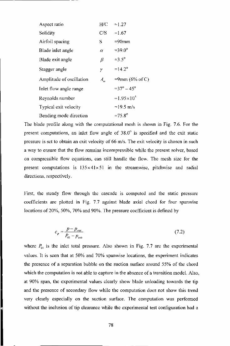
Aspect ratio H/C =1.27

Solidity CIS =1.67

Airfoil spacing s =90mm

Blade inlet angle a =39.0°

Blade exit angle fJ =3.5°

Stagger angle r =14.2°

Amplitude of oscillation Am =9mm ( 6% of C)

Inlet flow angle range =37°- 45°

Reynolds number =1.95 X 105

Typical exit velocity =19.5 rn/s

Bending mode direction =75.8°

The blade profile along with the computational mesh is shown in Fig. 7.6. For the

present computations, an inlet flow angle of 38.0° is specified and the exit static

pressure is set to obtain an exit velocity of 66 rn/s. The exit velocity is chosen in such

a way to ensure that the flow remains incompressible while the present solver, based

on compressible flow equations, can still handle the flow. The mesh size for the

present computations is 13 5 x 41 x 51 in the stream wise, pitch wise and radial

directions, respectively.

First, the steady flow through the cascade is computed and the static pressure

coefficients are plotted in Fig. 7.7 against blade axial chord for four spanwise

locations of20%, 50%, 70% and 90%. The pressure coefficient is defined by

C = p- Pexit

p p -01 Pexit

(7.2)

where Po 1 is the inlet total pressure. Also shown in Fig. 7.7 are the experimental

values. It is seen that at 50% and 70% spanwise locations, the experiment indicates

the presence of a separation bubble on the suction surface around 55% of the chord

which the computation is not able to capture in the absence of a transition model. Also,

at 90% span, the experimental values clearly show blade unloading towards the tip

and the presence of secondary flow while the computation does not show this trend

very clearly especially on the suction surface. The computation was performed

without the inclusion of tip clearance while the experimental test configuration had a

78

tip gap of 0.5 percent chord to accommodate the blade motion. The inlet total pressure

specification was based on the measured inlet total pressure profile which indicated

the presence of inlet boundary layer. The computed pressure coefficient for all

spanwise locations shows a somewhat jagged appearance on the suction surface, and

the reason for this is not clear. However, the overall agreement between the calculated

and the experimental values is good.

Having calculated the steady flow, the unsteady computation is performed for two

reduced frequencies of 0.4 and 0.6 (based on blade chord and isentropic exit velocity).

The amplitude specified at the tip is 6% of the blade chord. The bending amplitude is

varied linearly along the span from hub to tip. In order to confirm the linear behaviour

of the test configuration, the experimental tests were performed at two different

bending amplitudes, 6% and 3.3% of the blade chord. Fig. 7.7a shows the amplitude

and phase values of the unsteady pressure coefficient for these measurements and it

shows a nearly identical response for both amplitudes, thereby confirming the linear

behaviour. The unsteady results are presented at four span wise locations of 20%, 50%,

70% and 90% for three inter-blade phase angles of 90°, 180° and -90°. The unsteady

pressure coefficient is defined by

(7.3)

where A111

is the vibration amplitude at the tip. Fig. 7.8 to Fig. 7.11 show the

amplitude and phase of unsteady pressure coefficient for the reduced frequency of 0.4

and inter-blade phase angle of 90°. Also shown are the corresponding values from the

experiment. The calculation slightly under predicts the unsteady pressure load for the

forward 30% of the blade chord on both suction and pressure surfaces but this

gradually improves towards 90% of the span as the vibration amplitude increases. The

phase angle prediction shows a good agreement on the pressure surface while there is

a slight under prediction on the suction surface for all the span locations.

The amplitude and phase of unsteady pressure for inter-blade phase angle of 180° are

shown in Fig. 7.12 to Fig. 7.15. The calculation shows lower values for the amplitude

than that experimentally observed till 70% span, particularly on the suction surface,

indicating that the computation under predicts the effect of unsteadiness. The phase

79

predictions show a good agreement on the pressure surface and on the suction surface

the calculation is unable to predict the change in sign in the phase distribution due to

the separation bubble at 70% of the span.

For the inter-blade phase angle of -90°, the calculated unsteady pressure amplitude

and phase along with the experimental values are shown in Fig. 7.16 to Fig. 7.19. In

this case, the calculated values for the amplitude are slightly low compared to the

experimental values on the suction surface for up to 70% of the span. At the same

time, the pressure surface shows an over prediction between 20% and 40% of the

chord for all the spanwise sections. The phase angle predictions show reasonably

good agreement on the pressure surface for all the span locations while lower values

are predicted for the suction surface for 70% and 90% of the span locations. This

trend has been observed for all the three inter-blade phase angles. At 70% of the span,

for all three phase angles, the experimental values show a clear change in sign in the

phase distribution on the suction surface at around 55% of the chord due to the

presence of separation bubble and the numerical prediction is unable to capture this.

Having computed the unsteady pressure, how this affects the stability of the cascade

configuration should naturally be of interest and to determine this, the aerodynamic

damping coefficients are calculated for different inter-blade phase angles for the

reduced frequency 0.4. Fig. 7.20 shows the calculated damping values along with

experimentally determined values. It is seen the cascade configuration is stable for the

entire range of phase angles and the computation is able to predict this trend correctly.

Also, the values are slightly under predicted for all the phase angles except for -90°.

This is consistent with the under prediction of unsteady pressure loads. For the phase

angle -90°, while there is only a slight under prediction on the suction surface, the

over prediction on the pressure surface between 20% and 40% of the chord seems to

be contributing to a net amplitude that is higher than experimental value. Since the

phase angle prediction in this case is similar to that of other inter-blade phase angles,

the increase in damping can be attributed to the difference in pressure amplitude.

Next, the computational process is repeated for a reduced frequency of 0.6 and the

entire trend as regards the amplitude and phase of unsteady pressure is found to be

similar to that observed for reduced frequency 0.4. Therefore, for the sake of brevity,

80

those figures are not shown. However, the aerodynamic damping calculation is shown

in Fig. 7.21 and this shows that the stability margins have increased as expected at a

higher reduced frequency and the overall trend is similar to that observed for 0.4.

This entire exercise shows that the three-dimensional time-linearized Euler/Navier­

Stokes code is able to predict three-dimensional unsteady flows associated with blade

oscillations. Flutter is widely accepted as a linear phenomenon and the three­

dimensional test cases considered for the present computation are also of linear nature.

However, transonic unsteady flows involving shocks and their motions cause

significant nonlinear contributions to the local unsteady response associated with

blade flutter. As three-dimensional test data for such cases are not readily available,

the present work has not included any nonlinear flutter problems.

81

Chapter 8

Conclusions and Suggestions

The present work is concerned with the development of efficient frequency domain

methods for the prediction of three-dimensional unsteady turbomachinery flows. A

three-dimensional Navier-Stokes solver has been developed incorporating the time­

linearized method and nonlinear harmonic method. Some numerical investigations

have been carried out towards understanding and predicting unsteady flows in

turbomachinery with specific attention to flows around oscillating blades. These

investigations have revealed the relative merits of the time-linearized method and the

nonlinear harmonic method in addressing linear and nonlinear unsteady flows. Since

three-dimensional numerical investigations are constrained by the lack of

corresponding experimental data to validate them, those investigations have been

carried out to the extent possible and in all the other cases two-dimensional

investigations have been made necessary to validate the underlying methods. The

following sections summarise the conclusions drawn from the present work and offer

some suggestions for future work.

8.1 Linear Harmonic Method

In the area of frequency domain methods, the time-linearized method is widely used

in two-dimensional inviscid and viscous calculations for unsteady flows in

turbomachinery. In addition, three-dimensional inviscid Euler calculations are also

performed wherever necessary. However, so far there has been no three-dimensional

Navier-Stokes calculation involving the time-linearized method. The present work

approached and implemented the development of three-dimensional time-linearized

method for Euler/Navier-Stokes equations as a baseline method for the development

of three-dimensional nonlinear harmonic method for Euler/Navier-Stokes equations.

In Chapter 4, a detailed description of the development of three-dimensional time­

linearized method has been presented. In this method, the unsteady flow is

decomposed into a steady flow plus a harmonically varying unsteady perturbation.

The process of linearization transforms the original unsteady Euler/Navier-Stokes

82

equations into two equations, a steady flow equation and a time-linearized

perturbation equation. A pseudotime time-marching technique is introduced to take

advantage of well-developed time-marching schemes. The numerical solution

technique involved a cell centred finite volume scheme for spatial discretization and a

four stage Runge-Kutta scheme for time integration. Nonreflecting boundary

conditions are applied for far-field boundaries and a slip wall boundary condition is

used for Navier-Stokes equations.

The validation of the time-linearized Euler/Navier-Stokes method has been carried out

in two steps. First, a set of two-dimensional cases comprising an oscillating flat plate

cascade, a high frequency forced response case induced by incoming wakes for a flat

plate cascade and an oscillating turbine cascade has been considered. For the

oscillating flat plate cascade and the high frequency incoming wakes, a good

comparison with LINSUB has been obtained. For the oscillating turbine cascade of

Fourth Standard Configuration, the calculated results compared reasonably well with

the experimental data. Secondly, a set of three-dimensional cases comprising an

oscillating flat plate cascade and an oscillating linear compressor cascade has been

considered. The agreement between the calculated Euler solution for the oscillating

flat plate cascade and the solutions from Namba's semi-analytical method has been

good. For the experimental case of oscillating linear compressor cascade, the

calculated Navier-Stokes solutions agree reasonably well with the experimental data.

The aerodynamic damping calculations show good agreement with experimental data

indicating a reasonable prediction of stability margins. Therefore, the three­

dimensional Euler/Navier-Stokes time-linearized method has been shown to predict

unsteady flows around oscillating blades reasonably well.

8.2 Nonlinear Harmonic Method

The nonlinear harmonic method to predict nonlinear unsteady flows, was proposed by

He ( 1996) and the two-dimensional prediction of nonlinear unsteady flows have been

carried out successfully by Ning (Ning, 1998, He and Ning, 1998). The present work

has extended the nonlinear harmonic Euler/Navier-Stokes method to three­

dimensional unsteady flows. Also, inclusion of higher order harmonic perturbations

through the harmonic balance technique has also been implemented. In order to

83

- -- ---------------

compute blade oscillation, the present work uses moving computational grid in three­

dimensions. The need to extrapolate the flow variables from the boundary of the grid

to the instantaneous location of the airfoil as done in the case of fixed grid solutions is

thereby eliminated. In the nonlinear harmonic method, the unsteady flow is

decomposed into a time-averaged flow and an unsteady perturbation. Due to the

nonlinearity of the unsteady equations, time-averaging produces extra unsteady stress

terms in the time-averaged equations which are evaluated from unsteady perturbations.

While the unsteady perturbations are obtained by solving the harmonic perturbation

equations, the coefficients of perturbation equations come from the solution of time­

averaged equation. The time-averaged equations and harmonic perturbation equations

interact with each other and this interaction is achieved through a strong coupling

procedure. The nonlinear effects are included in the coupled solution approach

between the time-averaged equation and the unsteady perturbation equation. The

numerical solution method for the nonlinear harmonic method is very similar to that

used in the time-linearized method.

In order to handle strong nonlinearity in the flow, the present work also includes a

harmonic balancing technique, as proposed by He (200 1 ), to include higher order

perturbations in the solution of nonlinear flows as the original nonlinear harmonic

method could handle only first order perturbations. This harmonic balancing

technique introduces cross coupling of higher order perturbations which in tum

improves the accuracy of the fundamental harmonic through interaction with the time­

averaged equation. In the absence of higher order perturbations, the harmonic

balancing technique reduces to that of the first order perturbation equation of the basic

nonlinear harmonic method.

The validation of the nonlinear harmonic method has been carried out by calculating

transonic unsteady flows in a diverging channel and transonic flows through an axial

flow fan rotor subjected to inlet flow distortion. The calculation for the inviscid

transonic unsteady flows in a diverging channel has shown that the nonlinear

harmonic method can handle very strong levels of nonlinearity resulting from large

amplitude shock oscillation. The calculated values have been compared with solutions

from nonlinear time-marching method and time-linearized method. These

comparisons have shown that the validity of the time-linearized method for unsteady

84

flows is based on the strength of nonlinearity in the flow field. The nonlinear

harmonic method considerably improves the solution over the time-linearized method

in the presence of nonlinear effects. In addition, the inclusion of higher order

perturbations has enabled the nonlinear harmonic method to predict the strong

nonlinearity on a par with the nonlinear time-marching method. On the other hand,

the limitation of the nonlinear harmonic method has been observed from the

calculated results for inlet distortion through a transonic axial flow fan rotor. These

calculations have shown that the nonlinear harmonic method has a tendency to

amplify the nonlinearity in situations like oscillating shock interacting with the

boundary layer.

In terms of computational cost, the nonlinear harmonic method consumes 75% of

CPU time more than the time-linearized analysis, but it is still more efficient than the

nonlinear time-marching method for a similar calculation even after the inclusion of

cross coupling of higher order perturbations.

8.3 Suggestions for Future Work

Based on the limitations observed for the nonlinear harmonic method, it is imperative

to address the linearization of the turbulence viscosity in the perturbation equations.

The present practice of freezing the viscosity to its steady value seems to pose

problems in cases of strong viscous displacement effects. Also, the current form of

linearization of the pressure sensor in the numerical smoothing needs to be refined, to

handle flows with strong nonlinearity.

As far as unsteady predictions are concerned, the three-dimensional blade flutter

analysis problem can be approached to address nonlinear effects by including large

amplitude oscillations or by considering transonic flows with strong shock motions.

Since nonlinear harmonic method can handle perturbation from multiple sources of

unsteadiness, the blade flutter analysis could also include other sources of

tmsteadiness such as inlet distortions, bladerow interactions etc. In addition, some

more cases of three-dimensional blade flutter and forced response problems can be

considered for validation. The three-dimensional unsteady flow prediction will have a

85

number of applications m the area of flutter and forced response prediction and

analysis in the future.

86

References

Abhari, R.S. and Giles, M., 1997, "A Navier-Stokes Analysis of Airfoils in

Oscillating Transonic Cascades for the Prediction of Aerodynamic Damping," ASME

Journal ofTurbomachinery, Vol. 199, pp. 77-84

Adamczyk, J.J., 1985, "Model Equations for Simulating Flows m Multistage

Turbomachinery," ASME Paper 85-GT-226

Adamczyk, J.J., 2000, "Aerodynamic Analysis of Multistage Turbomachinery Flows

in Support of Aerodynamic Design," ASME Journal ofTurbomachinery, Vol. 122, pp.

189-217

Arnone, A., and Pacciani, R., 1998, "IGV -Rotor Interaction Analysis in a Transonic

Compresor Using the Navier-Stokes Equations," ASME Journal of Turbomachinery,

Vol. 120, pp. 147-155

Ayer, T.C., and Verdon, J.M., 1998, "Validation of a Nonlinear Unsteady

Aerodynamic Simulator for Vibrating Blade Rows," ASME Journal of

Turbomachinery, Vol. 120, pp. 112-121

Baldwin, B.S., and Lomax, H., 1978, "Thin-Layer Approximation and Algebraic

Model for Separated Turbulent Flow," AIAA Paper 78-257

Bell, D.L. and He, L., 2000, "Three-Dimensional Unsteady Flow for an Oscillating

Turbine Blade and the Influence of Tip Leakage," ASME Journal ofTurbomachinery,

Vol. 122, pp. 93-101

Boles, A., and Fransson, T.H., 1986, "Aeroelasticity in Turbomachines, Comparison

of Theoretical and Experimental Cascade Results," Communication du Laboratoire de

Thermique Appliquee et de Turbomachines, No. 13, Lausanne, EPFL

Carstens, V., and Belz, J., 2000, "Investigation of Fluid-Structure Interaction in

Vibrating Cascades Using a Time-Domain Method," Proceedings of the 9th

International symposium on Unsteady Aerodynamics, Aeroacoustics and

Aeroelasticity, eds, P. Ferrand and S. Aubert, pp.678-694

Carta, F.O., 1967, "Coupled Blade-Disc-Shroud Flutter Instabilities in Turbojet

Engine Rotors," ASME Journal of Engineering for Power, Vol. 89, pp. 419-426

Carta, F.O., and StHilaire, A.O., 1980, Effect of Inter-blade Phase Angle and

Incidence Angle on Cascade Pitching Stability," ASME Journal of Engineering for

Power, Vol. 102, pp. 391-396

87

Carta, F.O., 1983, "Unsteady Aerodynamics and Gapwise Periodicity of Oscillating

Cascaded Airfoils," ASME Journal of Engineering for Power, Vol. 105, pp. 565-574

Chassaing, J.C., and Gerolymos, G.A., 2000, "Compressor Flutter Analysis Using

Time-Nonlinear and Time-Linearized 3-D Navier-Stokes Methods," Proceedings of

the 9111 International symposium on Unsteady Aerodynamics, Aeroacoustics and

Aeroelasticity, eds, P. Ferrand and S. Aubert, pp. 666-677

Chen, T., Vasanthakumar, P. and He, L., 2000, "Analysis of Unsteady Blade Row

Interaction Using Nonlinear Harmonic Approach," AIAA Journal of Propulsion and

Power, Vol. 17, No.3, pp. 601-608

Clark, W.S., and Hall, K.C., 2000, "A Time-Linearized Navier-Stokes Analysis of

Stall Flutter," ASME Journal ofTurbomachinery, Vol. 122, pp. 467-476

Dawes, W.N., 1988, "Development of a 3D Navier-Stokes Solver for Application to

All Types ofTurbomachinery," ASME Paper 88-GT-70

Denton, J.D., 1983, An Improved Time-Marching Method for Turbomachinery Flow

Calculation," ASME, Journal ofEngineering for Power, Vol. 105, pp. 514-524

Denton, J.D., 1992, "The Calculation of Three-Dimensional Viscous Flow Through

Multistage Turbomachine", ASME Journal of Turbomachinery, Vol. 114, No. 1, pp.

18-26

Dorney, D.J., and Sharma, O.P., 1997, "Evaluation of Flow Field Approximations for

Transonic Compressor Stages", ASME Journal of Turbomachinery, Vol. 119, pp.

445-451

Erdos, J.l., Alzner, E., and McNally, W., 1977, "Numerical Solution of Periodic

Transonic Flow Through a Fan Stage," AIAA Journal, Vol. 15, No.l1, pp. 1559-1568

Gerolymos, G.A., 1988, "Numerical Integration of the Blade-to-Blade Surface Euler

Equations in Vibrating Cascades," AIAA Journal, Vol. 26, No. 12, pp. 1483-1492

Gerolymos, G.A., 1993, "Advances in the Numerical Integration of the Three­

Dimensional Euler Equations in Vibrating Cascades," ASME Journal of

Turbomachinery, Vol. 115, pp. 781-790

Giles, M.B., 1988, "Calculation of Unsteady Wake/Rotor Interaction", AIAA Journal

of Propulsion and Power, Vol. 4, pp.356-362

Giles, M.B., 1990a, "Stator/Rotor Interaction in A Transonic Turbine", Journal of

Propulsion and Power, Vol.6, No.5, pp.621-627

Giles, M.B, 1992, "An Approach for Multi-stage Calculations Incorporating

Unsteadiness", ASME Paper 92-GT-282

88

Giles, M.B., 1993, "Validation of a Numarical Method for Unsteady Flow

Calculations," ASME Journal of Turbomachinery, Vol. 115, pp. 110-117

Gruber, B, and Carstens, V ., 1998, "Computation of the Unsteady Transonic Flow in

Harmonically Oscillating Turbine Cascades Taking into Account Viscous Effects,"

ASME Journal ofTurbomachinery, Vol. 120, pp. 104-111

Hah, C., Rabe, D.C., Sullivan, T.J., and Wadia, A.R., 1998, "Effects of Inlet

Distortion on the Flow Field in a Transoinic Compressor Rotor," ASME Journal of

Turbomachinery, Vol. 120, pp. 233-246

Hall, E.J., 1997, "Aerodynamic Modeling of Multistage Compressor Flowfields- Part

2; Modelling Deterministic Stresses," ASME Paper 97-GT-345

Hall, K.C., and Crawley, E.F., 1989, "Calculation of Unsteady Flows in

Turbomachinery Using the Linearized Euler Euqations," AIAA Journal, Vol.27, No.6,

pp.777-787

Hall, K.C. and Lorence, C.B., 1993, "Calculation of Three-Dimensional Unsteady

Flows in turbomachinery Using the Linearized Harmonic Euler Equations,"

ASME.Journal ofTurbomachinery, Vol. 115, pp. 800-809

Hall, K.C., Clark, W.S., and Lorence, C.B., 1994, "A Linearized Euler Analysis of

Unsteady Transonic Flows in Turbomachinery," ASME Journal of Turbomachinery,

Vol. 116, pp. 477-488

Hall, K.C., Thomas, J.P. and Clark, W.S., 2002, "Computation of Unsteady Nonlinear

Flows in Cascades Using a Harmonic Balance Technique," AIAA Journal, Vol. 40,

No. 5, pp. 879-886.

He, L., 1990, "An Euler Solution for Unsteady Flows Around Oscillating Blades,"

ASME Journal ofTurbomachinery, Vol. 112, pp. 714-722

He, L., 1992, "A Method of Simulating Unsteady Turbomachinery Flows With

Multiple Perturbations," AIAA Journal, Vol. 30, No. 12, pp. 2730-2735

He, L., 1993, "A New Two Grid Acceleration Method for Unsteady Navier-Stokes

Calculations, AIAA Journal of Propulsion and Power, Vol. 9, No.2

He, L., 1994, "Integration of Two-Dimensional Fluid/Structure Coupled System for

Calculations of Turbomachinery Aerodynamic/ Aeroelastic Instabilities," Intl. Jl. of

Computational. Fluid Dynamics, Vol. 3, pp. 217-231

He, L. and Denton, J.D., 1994, "Three-Dimensional Time-Marching Inviscid and

Viscous Solutions for Unsteady Flows Around Vibrating Blades," ASME Journal of

Turbomachinery, Vol. 116, pp. 469-476

89

He, L., 1996, "Modelling Issues for Computation of Unsteady Turbomachinery

Flows," Unsteady Flows in Turbomachines, VKI Lecture Series 1996-05, von

Karman Institute for Fluid Dynamics.

He, L., and Ning, W., 1998, "Efficient Approach for Analysis of Unsteady Viscous

Flows in Turbomachines," AIAA Journal, Vol.36, No.11, pp. 2005-2012

He, L., 1999, "Nonlinear Time-Domain Aerodynamic Solutions," Aeroelasticity in

Axial-Flow Turbomachines, VKI Lecture Series 1999-05, von Karman Institute for

Fluid Dynamics.

He, L., 2001, University of Durham, Private Communication

Holmes, D.G., and Lorence, C.B., 1997, "Three-Dimensional Linearized Navier­

Stokes Calculation for Flutter and Forced Response," Proceedings of the 81h

International Symposium on Unsteady Aerodynamics and Aeroelasticity of

Turbomachines, ed. T.H. Fransson, Kluwer Academic Publishers, pp. 211-224

Isomura, K., and Giles, M.B., 1998, "A Numarical Study of Flutter in a Transonic

Fan,'"'ASME Journal ofTurbomachinery, Vol. 120, pp. 500-507

Jameson, A., Schmidt, W., and Turkel, E., 1981, "Numerical Solutions of the Euler

Equation by Finite Volume Method Using Runge-Kutta Time-stepping Scheme,"

AIAA Paper No. 81-1259

Jameson, A., 1991, "Time Dependent Calculations Using Multigrid With application

to Unsteady Flows Past Airfoils and Wings," AIAA Paper No. 91-1596

Kielb, R.E., 1999, "Flutter Design Analysis," Aeroelasticity in Axial Flow

Turbomachines, VKI Lecture Series, 1999-05, von Karman Institute of Fluid

Dymanics.

Koya, M. and Kotake, S., 1985, "Numerical Analysis of Fully Three-Dimensional

periodic Flows Through a Turbine Stage," ASME Journal of Engineering for Gas

Turbine and Power, Vol. 107, pp. 945-952

Lane, F., 1956, "System Mode Shapes in the Flutter of Compressor Blade Rows,"

Journal ofthe Aeronautical Sciences, Vol. 23, No.1, pp. 54-66

Li, H.D., and He, L., 2002, "Single Passage Analysis of Unsteady Flows around

Vibrating Blades of a Transonic Fan under Inlet Distortion," ASME Journal of

Turbomachinery, Vol. 124, pp. 285-292

Lindquist and Giles, M.B., 1994, "Validity of Linearized Unsteady Euler Equations

With Shock Capturing," AIAA Journal, Vol. 32, No. 1, pp. 46-53

90

Marshall, J.G., and Imregun, M., 1996, "An Analysis ofthe Aeroelastic Behaviour of

a Typical Fan Blade with Emphasis on the Flutter Mechanism," ASME Paper 96-GT-

78

Marshall, J.G., and Giles, M.B., 1997, "Some Applications of a Time-Linearized

Euler Method to Flutter & Forced Response in turbomachinery," Proceedings of the

8th International Symposium on Unsteady Aerodynamics and Aeroelasticity of

Turbomachines, ed. T.H. Fransson, Kluwer Academic Publishers, pp. 225-240

Morreti, G., and Abbett, M., 1966, "A Time-Dependent Computational Method for

Blunt Body Flows," AIAA Journal, Vol. 4, No. 12, pp. 2136-2141 Ni, R.H., and Sisto,

F., 1976, "Numerical Computation of Nonstationary Aerodynamics of Flat Plate

Cascades in Compressible Flows," ASME Journal of Engineering for Power, Vol. 98,

pp. 165-170

Namba, M., 1977, "Three-Dimensional Analysis of Blade Force and Sound

Generation for an Annular Cascade in Distorted Flows," Journal of sound and

Vibration, Vol. 50, pp. 479-508

Namba, M., and Ishikawa, A., 1983, "Three-Dimensional Aerodynamic

Characteristics of Oscillating Supersonic and Transonic Annular Cascades," ASME

Journal of Engineering for Power, Vol. 105, pp. 138-146

Namba, M., 1991, Kyushu University, Private Communication

Ni, R.H., 1982, A Multiple Grid Scheme for solving Euler Equations," AIAA Journal,

Vol.20,No.ll,pp.1565-1571

Ni, R.H., 1989, "Prediction of Multistage Turbine Flow Filed Using a Multiple Grid

Euler Solver, AIAA Paper No. 89-0203

Ning, W., 1998, "Computation of Unsteady Flow in Turbomachinery," Ph.D. Thesis,

University ofDurham

Ning, W. and He, L., 1998, "Computation of Unsteady Flows Around Oscillating

Blades Using Linear and Non-Linear Harmonic Euler Methods," ASME Journal of

Turbomachinery, Vol.120, pp.508-514

Platzer, M.F., and Carta, F.O., eds., 1988, "AGARD Manual on Aeroelasticity in

Axial Flow Turbomachines, Vol.2 - Structural Dynamics and Aeroelaticity

Rai, M.M., 1987, "Navier-Stokes Simulations of Rotor-Stator Interaction Using

Patched and Overlaid Grids," AIAA Journal of Propulsion and Power, Vol. 3, No. 5,

pp. 387-396

91

Rai, M.M., 1989, "Three-Dimensional Navier-Stokes Simulations of Turbine Rotor­

Stator Interaction", AIAA Journal of Propulsion and Power, Vol.5, No.3, pp.305-319

Rhie, C.M., Gleixner, A.J., Spear, D.A., Fischberg, C.J. and Zacharias, R.M., 1998,

"Development and Application of a Multistage Navier-Stokes Solver, Part 1:

Multistage Modelling Using Bodyforces and Deterministic Stresses", ASME Journal

ofTurbomachinery, Vol. 120, pp. 205-214

Saxer, A.P., and Giles, M.B., 1993, "Quasi-Three-Dimensional Nonreflecting

Boundary Conditions for Euler Equation Calculations," AIAA Journal of Propulsion

and Power, Vol. 9, No.2, pp. 263-271

Sisto, F., 1977, "A Review of Fluid Mechanics of Aeroelasticity in Turbomachines,"

ASME Journal of Fluids Engineering, Vol. 99, pp. 40-44

Silkowski, P.D., and Hall, K.C., 1998, "A Coupled Mode Analysis of Unsteady

Multistage Flows in Turbomachinery," ASME Journal of Turbomachinery, Vol. 120,

pp. 410-421

Srinivasan, A.V., 1997, "Flutter and Resonant Vibration Characteristics of Engine

Blades," ASME IGTI Scholar Paper 97-GT-533

Verdon, J.M., and Casper, J.R., 1982, "Development of a Linear Unsteady

Aerodynamic Analysis for Finite-Deflection Subsonic Cascades," AIAA Journal, Vol.

20, NO.9, pp. 1259-1267

Verdon, J.M., and Caspar, J.R., 1984, "A Linearized Unsteady Aerodynamic

Ananlysis for Transonic Cascades," Journal of Fluid Mechanics, Vol. 149, pp. 403-

429

Verdon, J.M., 1993, "Review of Unsteady Aerodynamic Methods for

Turbomachinery Aeroelastic and Aeroacoustic Applications," AIAA Journal, Vol. 31,

No.2, pp. 235-250

Whitehead, D.S., 1987, "Classical Two-Dimensional Methods," AGARD Manual on

Aeroelasticity m Axial Flow Turbomachines, Unsteady Turbomachinery

Aerodynamics, Vol. 1, AGARD-AG-298

Wood, J.R., Strazisar, A.J., and Hathaway, M.D., 1990, "Test cases for Computation

of Internal Flows in Aero Engine Components, Test Case- E/C0-2: Single Transonic

Fan Rotor," AGARD-AR-275

Yang, H., 2000, "An Experiment on 3D Unsteady Flow in a Linear Oscillating

Compressor Cascade," First Year Report, School of Engineering, University of

Durham

92

Yang, H., and He, L., 2002, "Experiment on Linear Compressor Cascade with 3-D

Blade Oscillation," ASME03-GT2003-38484, Communicated.

93

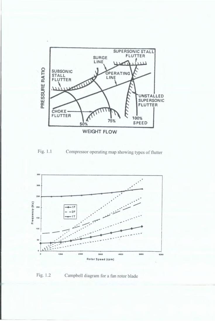
Fig. 1.1

SUBSONIC STALL FLUTTER

'

SUPERSONIC STALL

50%

WEIGHT FLOW

FLUTTER f

UNSTALLED SUPERSONIC FLUTTER

100% SPEED

Compressor operating map showing types of flutter

360.------------------------,

%SO L-----------:-7 ... e. 200 >-.. c: • :I

~ .so r u. 100 l

!

Fig. 1.2

.--: -;.,. .. . . .

Rotor Speed (rpm)

..

-~--- .. --...

uoo

Campbell diagram for a fan rotor blade

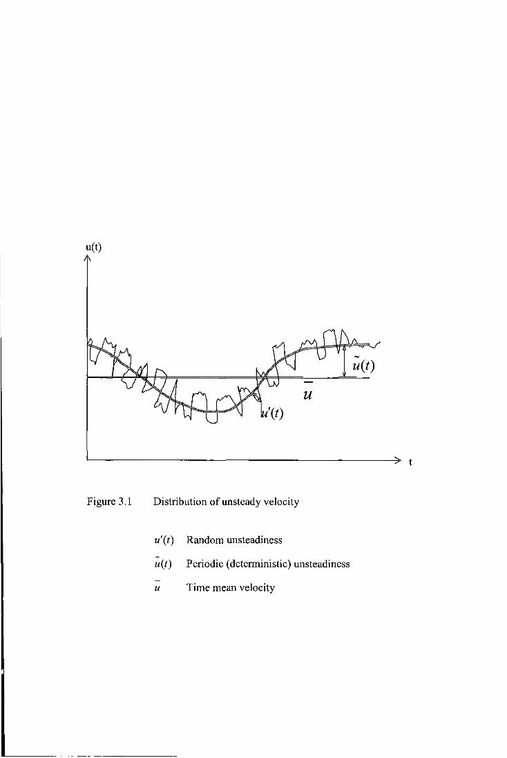
u(t)

-u(t)

u

t

Figure 3.1 Distribution of unsteady velocity

u'(t) Random unsteadiness

u(t) Periodic (deterministic) unsteadiness

u Time mean velocity

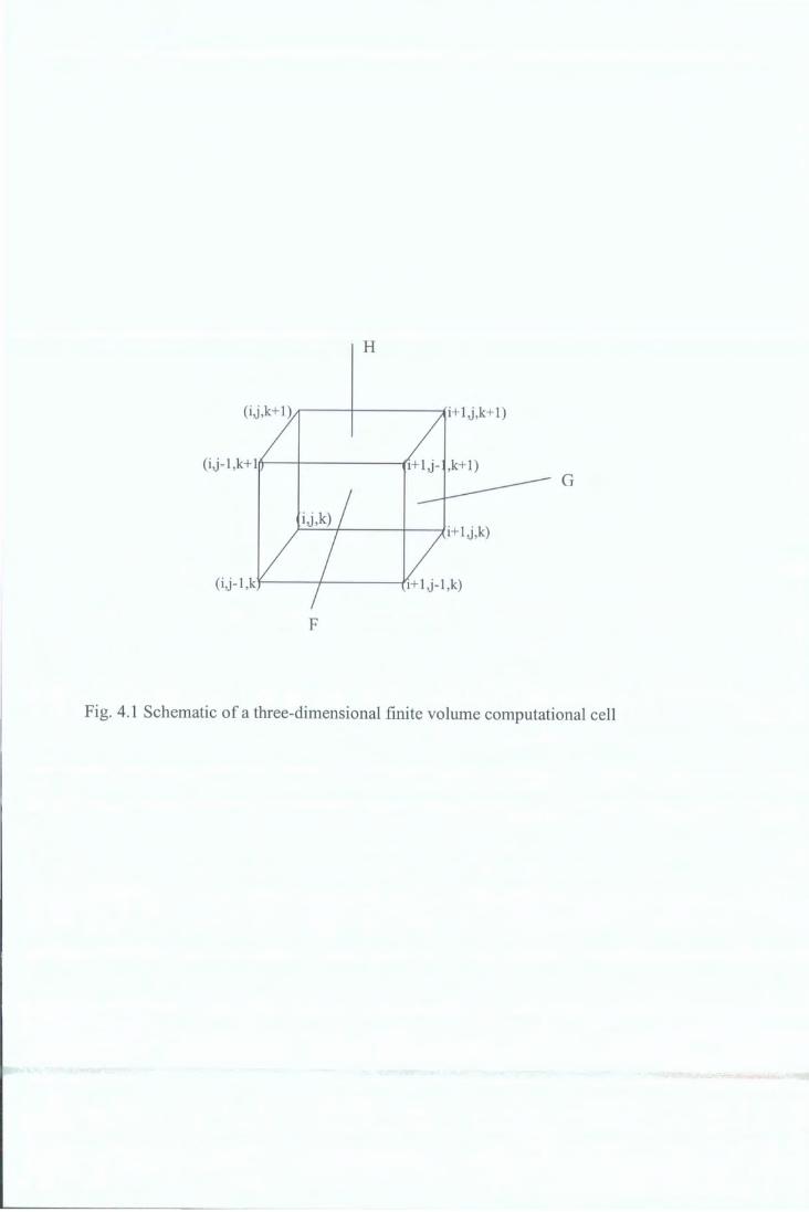
H

(i,j-1 ,k+ 1~-t------11

G

F

Fig. 4.1 Schematic of a three-dimensional finite volume computational cell

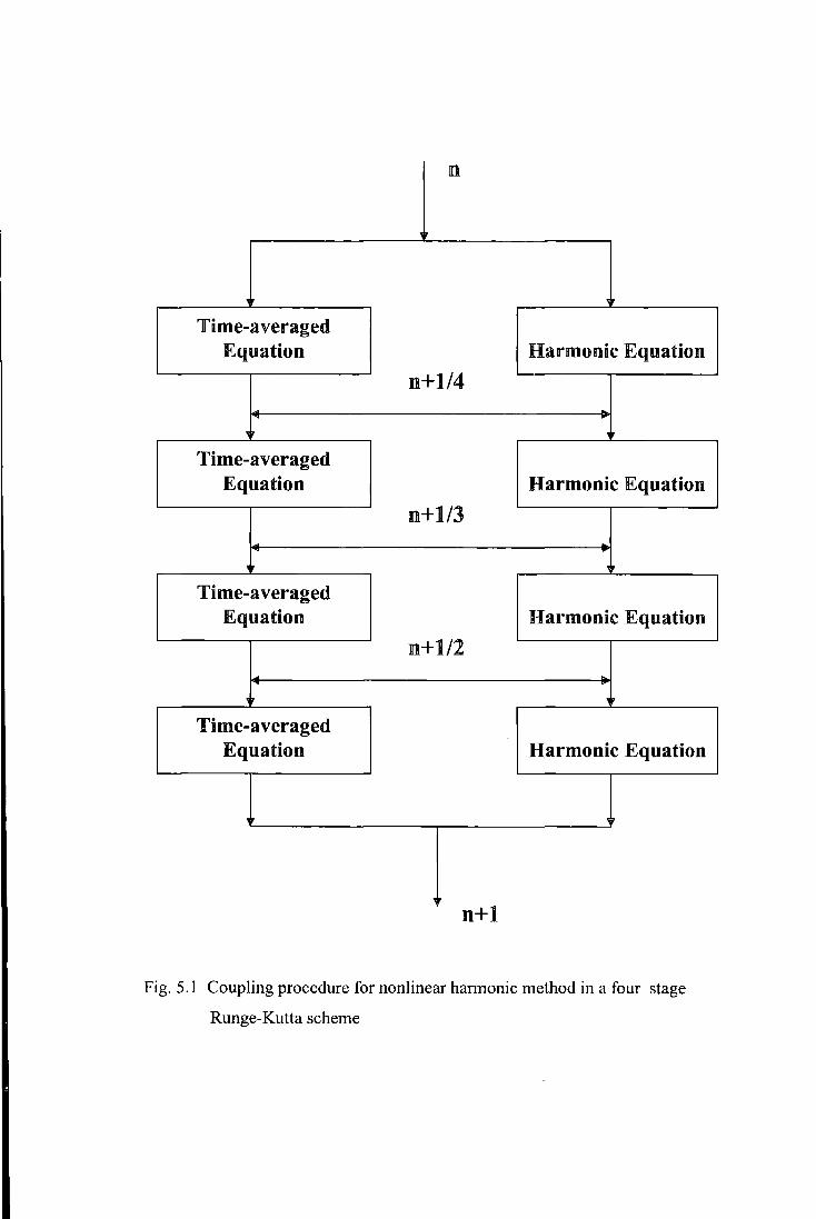
n

'fime=averaged JEquation Harmonic Equation

n+l/4

Time-averaged Equation Harmonic Equation

n+ 1/3

Time-averaged Equation Harmonic Equation

n+l/2

Time-averaged Equation Harmonic Equation

n+l

Fig. 5.1 Coupling procedure for nonlinear harmonic method in a four stage

Runge-Kutta scheme

IBPA=90 deg 20~-------------------------------------.

15 -c Q) 10 ·o ~

~ 5

() c.. 0

E ~ -5

~ ::J -10

~ ct -15

• Lin sub (Real) 0 Linsub (Imaginary)

--- Calculation (Real) , ~alculation (Imaginary) \ • "'&

----------~-

-20 +---.--...--....---...--....---...--....---...--..----i 0.0 0.2 0.4 0.6 0.8 1.0

X/C

IBPA=180 deg 20,--------------------------------------,

15 -c Q) 10 ·o ~

~ 5

() c.. 0 E ~ -5

~ ::J -10 ~ ~ 0.. -15

\

'•

• Linsub (Real) 0 Linsub (Imaginary)

--- Calculation (Real} ~lculation (Imaginary)

.. , .. ______ Jl __ • __ • __ • •

-- --

-20 +---.---.----.---..----.--...--....---..---.,...--1 0.0 0.2 0.4 0.6 0.8 1.0

X/C

Fig 6.1 Real and imaginary parts of unsteady pressure jump coefficient for a flat plate cascade (Bending; Reduced frequency=l.O)

IBPA=-90 deg 20,---------------------------------------

15 .... c Q) 10 ·o !:E ~ 5

(.) a. 0 E ~ ·5

~ :::J -10

~ ~ 0.. -15

00 0.2 0.4

• Linsub (Rea I) 0 Linsub (Imaginary)

- -- Ca leu Ia tion (Real) ----ca leu Ia tion (Imaginary)

0.6 0.8

X/C

IBPA=O deg

1.0

20,--------------------------------------,

15

c Q) 10 ·o !:E ~

(.)

5

a. 0 E ~ -5

~ :::J -10

~ ~ 0.. -15

• Linsub (Real) 0 Linsub (Imaginary)

- - - Calculation (Real) ---Calculation (lmagin ary)

-20 +-""T'"""-""T'"""--r---r---r---,----,----.----.-----j

0.0 0.2 0.4 0.6 0.8 1.0

X/C

Fig 6.2 Real and imaginary parts of unsteady pressure jump coefficient for a flat plate cascade (Bending; Reduced frequency=l.O)

-------------------------------------- -- ----

-c Q) ·o !E Q) 0 ()

0.. E ::J ...., Q) ..... ::J

~ Q) ..... a_

-c Q) ·o !E Q) 0 () 0.. E ::J ...., Q) ..... ::J

~ Q) ..... a_

25

20

15

10 ' ~ ~~

5 If' .. ~ 'ir ..

0 oo -5

-10

-15

IBPA=90deg

~ Linsub (Real) 0 Linsub (Imaginary)

~ ~ ~ calculation (Real) ==calculation (Imaginary)

-20 -+---.----.----r---r---.----r---r--...--...-----1 0.0 0.2 0.4 0.6 0.8 1.0

X/C

I BPA=180 deg 25

' 1!!1 Linsub (Real) 20 D I 0 Linsub (lmagina ry)

15 D ~ ~ ~ Calculation (Real)

~ ~alculation (Imaginary) 10

'~ ........... 5

0

-5

-10

-15

-20 0.0 0.2 0.4 0.6 0.8 1.0

X/C

Fig 6.3 Real and imaginary parts of unsteady pressure jump coefficient for a flat plate cascade (Torsion; Reduced frequency=l.O)

I BPA=-90 deg 25~------------------------------------~

20

c Q) 15 ·o !E 10

~ 0 5 a. E o :::J ...., ~ -5

:::J ~ -10

~ a_ -15

• Linsub (Rea I) 0 Linsub (Imaginary)

- ~ - Ca leu Ia tion (Real) ~lculation (Imaginary)

-20+---.--.----.---,----.---,----.---,---...----1 0.0 0.2

25

20 -c 15 Q) ·o IE 10

~ 0 5

a. E 0 :::J ...., Q) -5 .._ :::J

~ -10 Q) .._

-15 a_

-20 0.0 0.2

0.4 0.6 0.8

X/C

IBPA=Odeg

0.4

• Linsub (Real) 0 Linsub (Imaginary)

- - • Calculation (Real) ......-.calculation (lmagin ary)

0.6 0.8

X/C

1.0

1.0

Fig 6.4 Real and imaginary parts of unsteady pressure jump coefficient for a flat plate cascade (Torsion; Reduced frequency=l.O)

3,-------------------------------------------,

2

-LL ~0 -c Q) -1

'(3

~ -2

0 (,) -3 Q) (.)

0 -4 LL

-5

• Linsub (Real) 0 Linsub (Imaginary)

- - - Calculation (Rea I) ~alculation (lmagina ry)

~~----~--~~--~--------~~---r----.-----r -180 -90 0 90 180

Phase

1.0

li Linsu b (Real)

0.5 0 Linsu b (Imaginary) - ---Calculation (Real)

2 ~alculation (Imaginary) (,) - 0.0 -c Q)

'(3 -0.5 ... .. ..

~ ...... ...... _ ... -

8 ... -... ... ... _ ..... ... • ... ... - -1.0 c Q)

E • 0 -1.5 2

-2.0 -180 -90 0 90

Phase

Fig 6.5 Force and moment coefficients for a flat plate cascade (Bending; Reduced frequency=l.O)

180

3

2 l<:l Li nsub (Real) 0 Linsub (Imaginary)

- ~ ~ ~ Calculation (Rea I) LJ.. ~alculation (Imaginary) (.)

0 --c 0 0 (].) -1 0 "(3

IE -2 t? ... t? ..

(].) .. 0 t? .... ~ru (.) t?

-3 t? .., .,"iiiii ..,

(].) .. (,) .. .. .. .. .... -4 "" "" .. .. 0 , ..

LJ.. .. -5 ~

-6 -180 -90 0 90 180

Phase

1.0

§ Linsub (Real)

0.5 0 Linsub (lmagina ry) - ~ ~ ~ Calculation (Real) ~ ~alculation (Imaginary) (.)

0.0 - " c .1?1!!1"' (].) .1? .. "(3 .1? ~

iE -0.5 t? ..

(].)

8 - -1.0 .. c ..... ~

.. 0 -1.5 ~

-2.0 -180 -90 0 90 180

Phase

Fig 6.6 Force and moment coefficients for a flat plate cascade (Torsion; Reduced frequency=l.O)

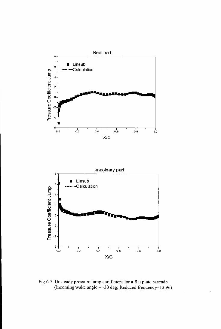
8

6 a. E :::J ...., 4

-c Q) 2 ·u !E ~ 0

(.) Q) ..... -2 :::J f/) f/)

~ -4 a_

-6 0.0

8

6 a. E ::J ...., 4

..... c Q) 2 ·u !E Q)

0 0 (.) Q) ..... -2

~ f/) Q)

-4 ..... a_

-6

0.0

Real part

• Linsub -----calculation

0.2 0.4 0.6

X/C

Imaginary part

• Linsub --........calculation

0.2 0.4 0.6

X/C

0.8 1.0

0.8 1.0

Fig 6. 7 Unsteady pressure jump coefficient for a flat plate cascade (Incoming wake angle= -30 deg; Reduced frequency=13.96)

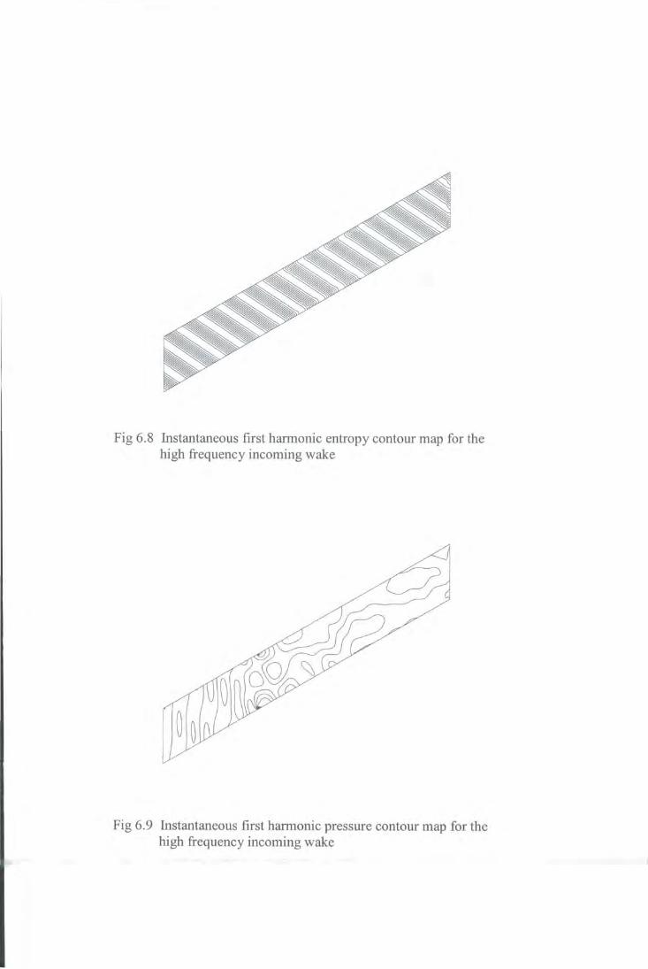
Fig 6.8 Instantaneous first harmonic entropy contour map for the high frequency incoming wake

Fig 6.9 Instantaneous first harmonic pressure contour map for the high frequency incoming wake

1.4

I... 1.2 Q)

..0 E ::::::1

z ..c (.)

ro ~ .S:2 a. 0 I... -c Q) (J)

1.0

0.8

0.6

0.4

0.2

0.0

Ill Experiment (Pressure surface) A E.xp eriment (Suction surface)

"' ..... Calculation (Pressure surface) -----Ga leu Ia tion (Suction surface)

0.0 0.2 0.4 0.6

XJC 0.8 1.0

Fig. 6.10 Isentropic Mach number distribution for a turbine cascade (Fourth Standard Configuration)

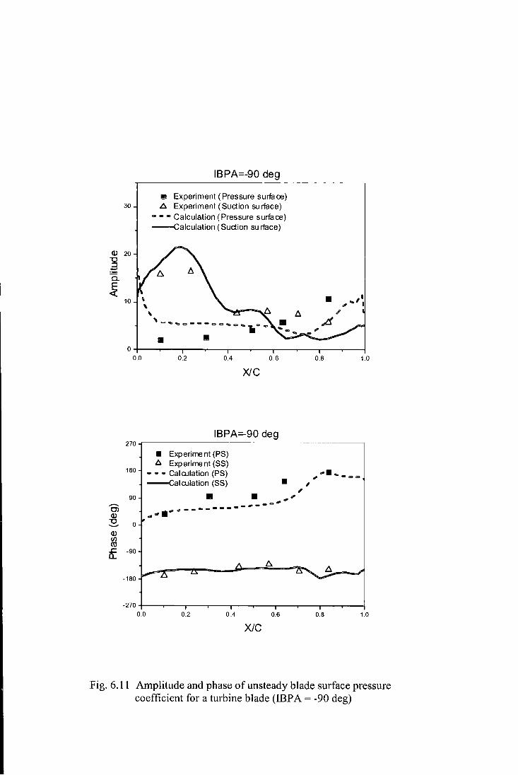
IBPA=-90 deg

111 Experiment (Pressure surface) 30 A Experiment (Suction surface)

<1) 20 "0 .3

10

0.0

~--Calculation (Pressure surface) ~alculation (Suction surface)

0.2 0.4 0.6

XJC

0.8 1.0

Fig. 6.11 Amplitude and phase of unsteady blade surface pressure coefficient for a turbine blade (IBP A = -90 deg)

IBPA=90 deg

!§I Experiment (Pressure surface) 30 6. Experiment (Suction surface)

~~~Calculation (Pressure surface) ===Calculation (Suction surface)

Q) 20 -g :!::::: a.

~ 10

Iii II

Iii 0 0.0 0.1 0.2 0.3 0.4 0.5 0.6 0.7 0.8 0.9 1.0

XJC

IBPA=90 deg 270~---------------------------------------,

Iii Experiment (PS) L:l. Experiment (SS)

180 ---Calculation (PS) ~alculatio n (SS)

90

-270 +----.---,---.-----.---.---y----..,.----r-----r----l 0.0 0.2 0.4 0.6 0.8 1.0

X/C

Fig. 6.12 Amplitude and phase ofunsteady blade surface pressure coefficient for a turbine blade (IBP A = 90 de g)

30

Q) 20 "0 .a c.

~ 10

IBPA=180 deg

0 Experiment (Pressure surface) 6. Experiment (Suction surface)

o ~ ~ Calrulation (Pressure surface) ==Ca lrula lion (Suction surface)

o;---~--.---~--~--~--r---~--r---~~ 0.0 0.2 0.4 0.6 0.8 1.0

XJC

270 IBPA=180 deg

180 ,-= b. c:.. ,f!r , 90 !;I I , - 1!!1 I O'l

"'-~ liil Q) ., ... .. ~ 0

~CICI-=oCIOCIICICbc:tGa e.~- .. -Q) (J)

m Experiment (PS) co ..s::: -90 6. Experiment (SS) a..

- o o Galrulation (PS) _1'l.

-180 ..... - ==Calrulation (SS)

-270

0.0 0.2 0.4 0.6 0.8 1.0

X/C

Fig. 6.13 Amplitude and phase of unsteady blade surface pressure coefficient for a turbine blade (IBP A = 180 de g)

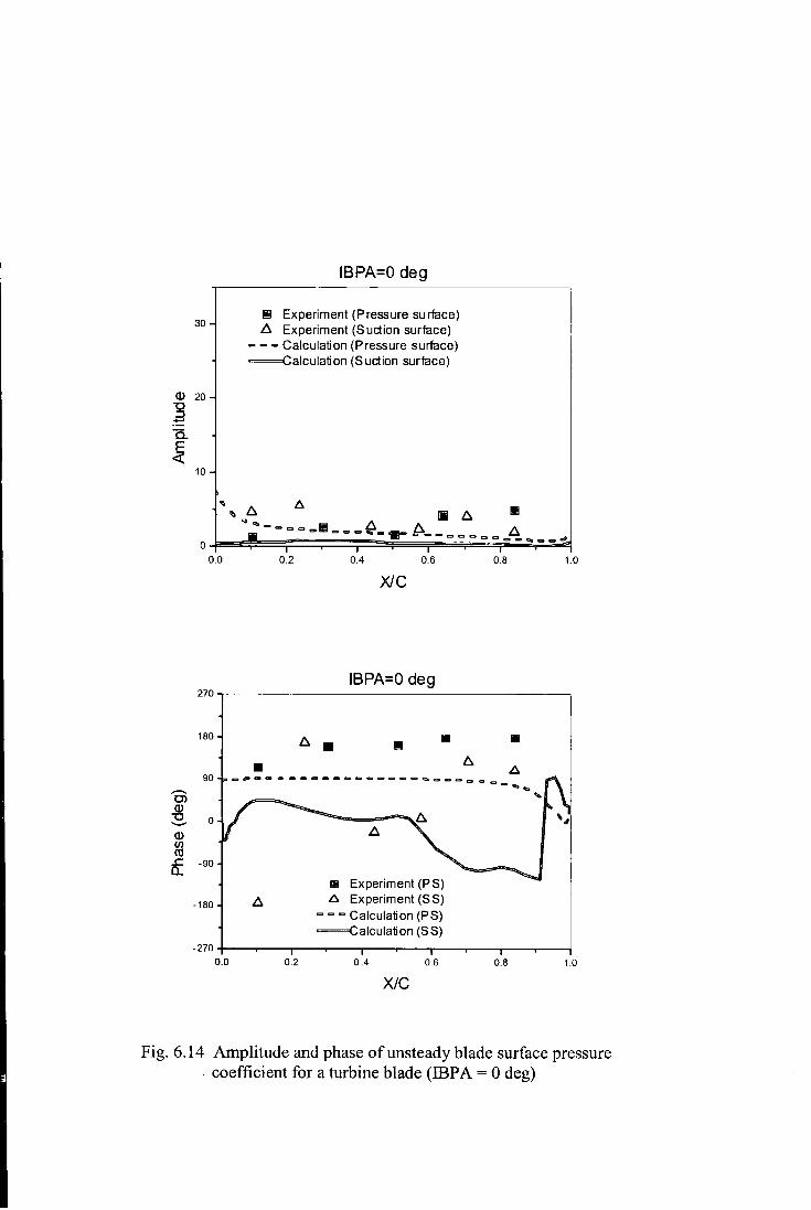
30

10

0.0

IBPA=O deg

~ Experiment (Pressure surface) l:::. Experiment (Suction surface)

~~~Calculation (Pressure surface) =Calculation (Suction surface)

0.2 0.4 0.6

XJC

IBPA=O deg

0.8 1.0

270~-------------------------------------,

180

90

C) Q)

~ 0 Q)

~ ..c -90 a.

-180

II 1!!1 Ill

• -p--0------------~~---a-­ ....

111 Experiment (P S) t::. Experiment (S S)

~~~Calculation (PS) ==Calculation (SS)

-270 +--~-.--...----.--...----,----r---y---,....----i 0.0 0.2 0.4 0.6 0.8 1.0

X/C

Fig. 6.14 Amplitude and phase of unsteady blade surface pressure coefficient for a turbine blade (IBPA = 0 deg)

------------------ --------- -

....... c Q) ·o !E Q) 0 0 0) c ·a. E ro

Cl C)

.E ro c >. "0 0 1....

~

12

Ill Experiment 10- - ... ..Calculation

8 ;. ...

6 " ~ ...

6' II ....

~', , .......

4

" ~ , 2

, I

" .. ' ""

""' d? "" 0 ""' ,"' Ill

~"" -2- Ill

-4

-6 I

-180 -90 0 90 180

lnterblade Phase Angle

Fig. 6.15 Aerodynamic damping coefficients in dependence of interblade phase angle (Fourth standard configuration)

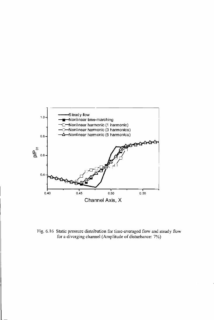
0 a..

1.0

0.8

'C. 0.6

0.4

0.40

"""""""""'oF.S tead y flow ~onlinear time-marching ---o--Nonlinear harmonic (1 harmonic) -:::>-Nonlinear harmonic (3 harmonics) ----6-Nonlinear harmonic (5 harmonics)

0.45 0.50

Channel Axis, X

0.55

Fig. 6.16 Static pressure distribution for time-averaged flow and steady flow for a diverging channel (Amplitude of disturbance: 7%)

10-

0.3

10 -c Q) ·a 8 t+= Qj 0 u 6

~ ::I 1/)

!fi 4 ,_ a.. >.

2 "'C

m -1/) c 0

:::::>

0.3

Real part

~onlinear time-marching = = = Linear harmonic ---6---Nonlinear harmonic (5 harmonics)

o, o a I \ I I I I

t\ 6i '~~ 0.4 0.5

Channel Axis, X

Imaginary part

~online ar time-marching ===Linear harmonic

0.6

----6-Nonlinear harmonic (5 harmonics)

0.4 0.5 0.6

Channel Axis, X

0.7

0.7

Fig. 6.17 First ham1onic unsteady pressure coefficient for a diverging channel (Amplitude of disturbance: 7%)

Real part 4,----------------------------------------,

----w-Nonli near time-marching ----b-Nonli near harmonic (5 harmonics)

1\ ~If ~~ ~

-3~--~----~----~---r----T---~----~--~ 0.3 0.4 0.5 0.6 0.7

Channel Axis, X

Imaginary part 4~---------------------------------------,

-Nonlinear time-marching c 3 -6-Nonlinearharmonic(Sharmonics) Q)

:~ ~ 2 Q) 0 u ~ :::J

~ o~~~~~'tf,r a.. >- -1

-g 2 -2 (/) c:

::::> -3~---T----,---~-----.----~---.----T---_,

0.3 0.4 0.5 0.6 0.7

Channel Axis, X

Fig. 6.18 Second harmonic unsteady pressure coefficient for a diverging channel (Amplitude of disturbance: 7%)

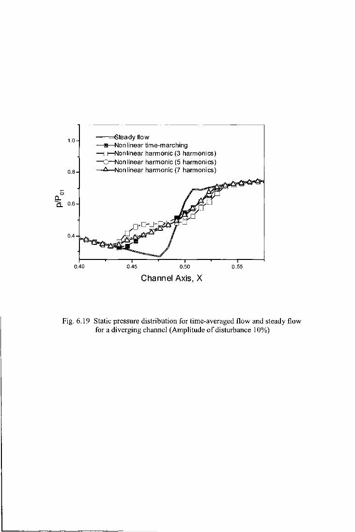
1.0 ==Btea dy flow ----M-Non linear time-marching -trNonlinear harmonic (3 harmonics) ---cr-Non linear harmonic (5 harmonics)

0.8 --.6--Non linear harmonic (7 harmonics)

~

0

a.. Ci. 0.6

0.4

0.40 0.45 0.50 0.55

Channel Axis, X

Fig. 6.19 Static pressure distribution for time-averaged flow and steady flow for a diverging channel (Amplitude of disturbance 1 0%)

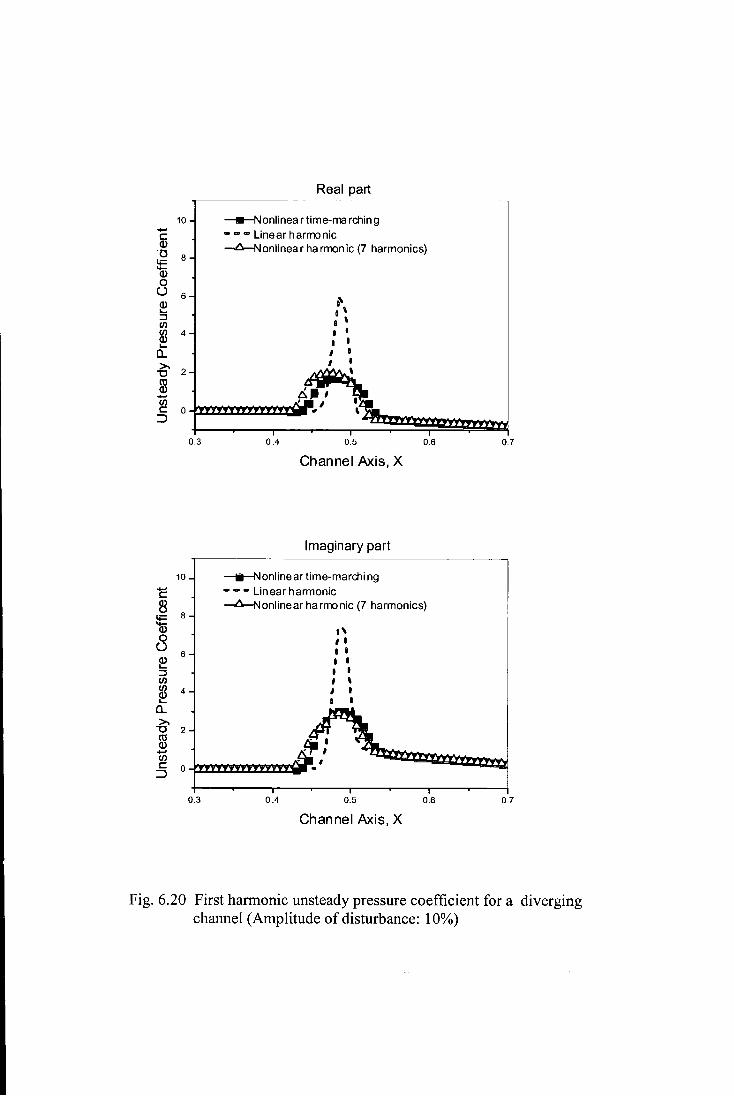
10 -c::

Real part

-Nonlinear time-rna rchin g ~~-Linear harmonic --.6-.Nonlinea r harmonic (7 harmonics) Q)

·o li= 8

'a> 0 u 6

•' ~ •' ~ a ' ~ 4 I I ._ I I ~ I I

~ 2 ~ m A~; ~ ~ o i:zmct:zm~m~,/.•'_.r: .. ' ~'-. :::::>

0.3 0.4 0.5 0.6

Channel Axis, X

Imaginary part

10 -w-N online ar time-marching ---Linear harmonic ~onlinearharmonic (7 harmonics)

0.3 0.4

1\ I I I I I I I I I \ I I I I

0.5

Channel Axis, X

0.6

0.7

0.7

Fig. 6.20 First harmonic unsteady pressure coefficient for a diverging channel (Amplitude of disturbance: 10%)

Real part 3~-------------------------------------.

~onlinea r time-marching - -----6-Nonlinearharmonic (7 harmonics) 53 2

-3~---T----.---~----.---~----.----r--_, 0.3 0.4 0.5 0.6 0.7

Channel Axis, X

Imaginary part 3~-------------------------------------.

~onlinea r time-marching ~onlinea r harmonic (7 harmonics)

-3 -f-----r-----,,-----.------.-----.-----r-----..-----1 0.3 0.4 0.5 0.6 0.7

Channel Axis, X

Fig. 6.21 Second harmonic unsteady pressure coefficient for a diverging channel (Amplitude of disturbance: 10%)

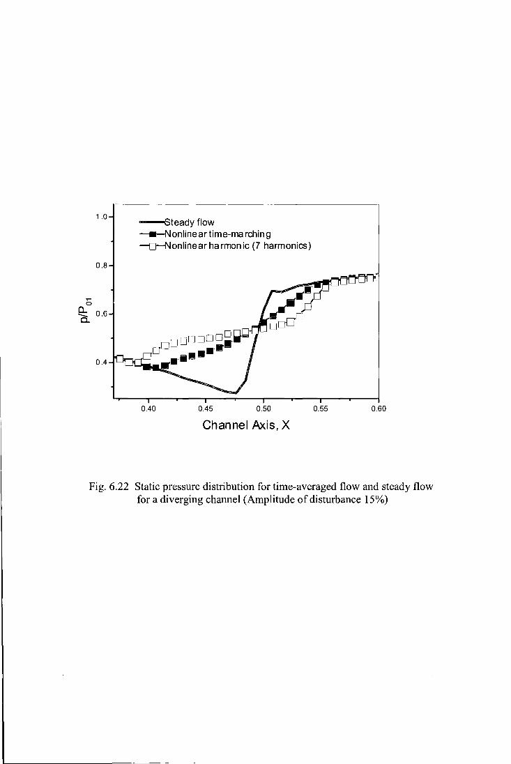
1 .0

0.8

0 a.. Ci 0.6

0.4

--steady flow --.-Nonlinear time-marching ---[]--Nonlinear harmonic (7 harmonics)

0.40 0.45 0.50 0.55 0.60

Channel Axis, X

Fig. 6.22 Static pressure distribution for time-averaged flow and steady flow for a diverging channel (Amplitude of disturbance 15%)

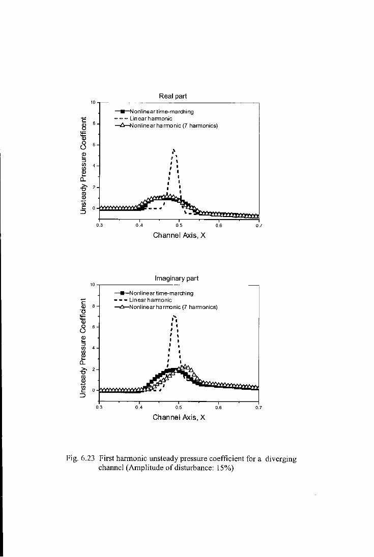
Real part 10,------------------------------------------,

0.3

---.-Nonlinear time-marching ~~~Linear harmonic ---6----Nonlinear harmonic (7 harmonics)

0.4

o' I ' I \ I I I I D I I I I I

0

0.5

Channel Axis, X

Imaginary part

0.6 0.7

10,-------------------------------------------

0.3

---.-Nonlinear time-marching ---Linear harmonic --oCr--Nonlinear harmonic (7 harmonics)

0.4

... I I I I I I I \ I I I •

I I

I I

0.5

Channel Axis, X

0.6 0.7

Fig. 6.23 First harmonic unsteady pressure coefficient for a diverging channel (Amplitude of disturbance: 15%)

Real part 3,----------------------------------------,

-G-Nonline ar time-marching ---.ll.--Nonline ar harmonic (7 harmonics)

AN\J'v,

-3~--~-----r----~---.----~--~----~--~ 0.3 0.4 0.5 0.6 0.7

Channel Axis, X

Imaginary part 3~---------------------------------------,

--!i!-Nonlinear time-rna rching --6-Nonlinear harmonic (7 harmonics)

-3~--~-----r----r----.----~--~----~--~ 0.3 0.4 0.5 0.6 0.7

Channel Axis, X

Fig. 6.24 Second harmonic unsteady pressure coefficient for a diverging channel (Amplitude of disturbance: 15%)

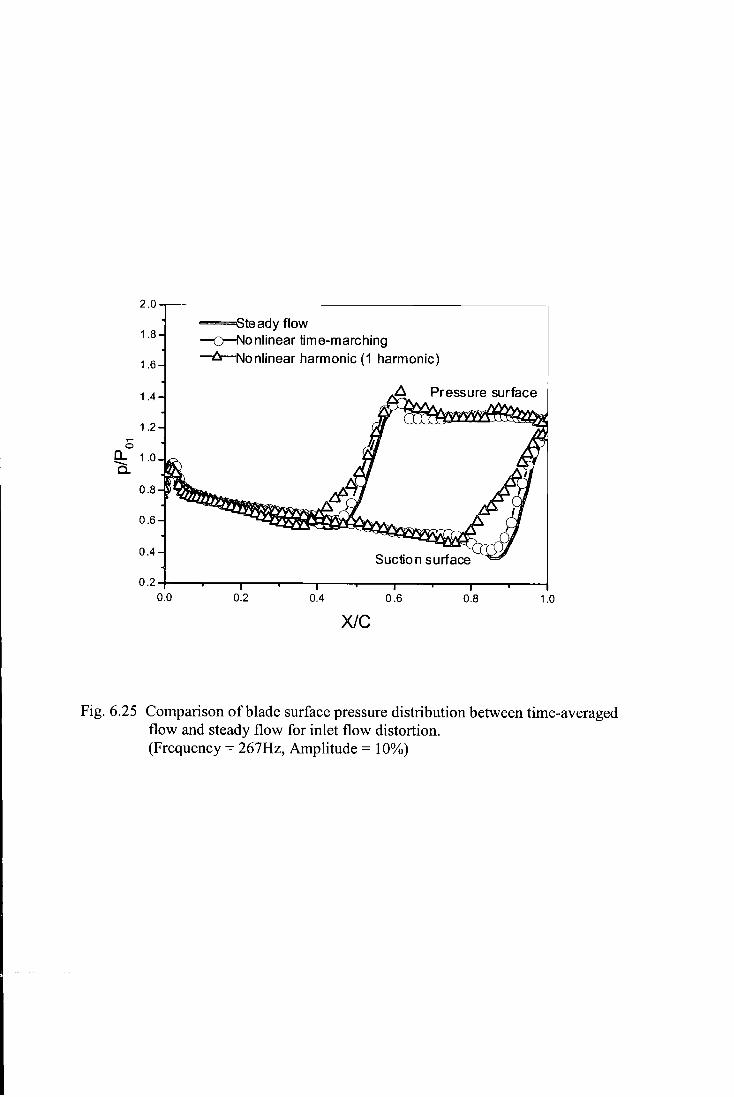
2.0

1 .8 """"'""""'...c::;ste ady flow ---cr-No nlinear time-marching

1 .6 -6--Nonlinear harmonic (1 harmonic)

1.4

1 .2 ~

0 a.. 1 .0 c. 0.8

0.6

0.4

0.2 0.0 0.2 0.4 0.6 0.8 1.0

X/C

Fig. 6.25 Comparison of blade surface pressure distribution between time-averaged flow and steady flow for inlet flow distortion. (Frequency= 267Hz, Amplitude= 10%)

Suction surface 40,-----------------------------------------,

30

Q)

-g 20 ......

10

0.0

-<rNonlinear time-mardling ====linear harmonic --6-Nonlinear harmonic (1 harmonic)

0.2 0.4 0.6

X/C

Pressure surface

0.8 1.0

40,------------------------------------------

Q) -o

30

2 20

c..

~ 10

0.0

--o-N online ar time-mardli ng ............j_in ear harmonic ~onlinear harmonic (1 harmonic)

0.2 0.4 0.6

X/C

0.8 1.0

Fig. 6.26 Amplitude of unsteady blade surface pressure coefficient for inlet flow distortion. (Frequency= 267Hz, Amplitude= 10%)

Suction surface 360

---crNonlinear time- marching

270 -i...inea r harmonic ~onlinear harmonic (1 harmonic)

180

Q) 90 (/)

ro ..c a..

0

-90

-180

0.0 0.2 0.4 0.6 0.8 1.0

X/C

Pressure surface 360

--0-Nonlinear time-rna rching

270 --Linear harmonic ----6---Nonlinear harmonic (1 harmonic)

180

Q) 90 (/)

ro ..c a..

0

-90

-180

0.0 0.2 0.4 0.6 0.8 1.0

X/C

Fig. 6.27 Phase of unsteady blade surface pressure coefficient for inlet flow distortion. (Frequency= 267Hz, Amplitude= 10%)

2.0

1 .8 ==6tea dy flow -o-Non linear time-marching

1 .6 --6-Nonlinear harmonic (1 harmonic)

1 .4

1 .2 ~

0 a.. 1 .0 c. 0.8

0.6

0.4

0.2 0.0 0.2 0.4 0.6 0.8 1.0

X/C

Fig. 6.28 Comparison ofblade surface pressure distribution between time-averaged flow and steady flow for inlet flow distortion. (Frequency = 1069Hz, Amplitude = 1 0%)

Q) "'C

Suction surface 40~---------------------------------------.

---<:rNonlinear time-mardling -Linear ha rrnon ic ----6-Nonlinear harmonic (1 harmonic)

30

.2 20

0..

~

Q) "'C

10

00 0.2 0.4 0.6 0.8 1.0

XJC

Pressure surface 40~---------------------------------------,

30

-<:rNo nlinear time-marching ~inear harmonic ---6--No nlinear harmonic (1 harmonic)

.2 20

a. ~

10

0~~~~~~~ 0.0 0.2 0.4 0.6 0.8 1.0

XJC

Fig. 6.29 Amplitude of unsteady blade surface pressure coefficient for inlet flow distortion. (Frequency= 1069Hz, Amplitude= 10%)

360

270

180

Q) 90 C/)

co ..c a..

0

-90

-180

0.0

360

270

180

Q) 90 C/)

co ..c a..

0

-90

-180

0.0

Suction surface

--crNo nlinear time-marching ===Linear harmonic -6-Nonlinear harmonic

0

~~ Q 0

0.2 0.4 0.6

X/C

Pressure surface

--o--No nlinear time-marching ~inear harmonic -6-Nonlinear harmonic (1 harmonic)

0.2 0.4 0.6

X/C

0.8 1.0

0.8 1.0

Fig. 6.30 Phase of unsteady blade surface pressure coefficient for inlet flow distortion. (Frequency= 1069Hz, Amplitude= 10%)

Real part R/S=O.O Imaginary part R/S=O.O 10 10

D Namba [] Namba --calculation

1: ---calculation

1: 6 6 Ql Ql ·o 4 ·o 4 IE IE 2l 2 2l 2

u 0~ u .a "' .. "" "' n g c. 0 J;'-

~ .:.. w ~ E

:J ·2 :J -2 -, -,

~ -4 ~ -4 :J :J

!ll -6 !ll .. Q) Ql

It .. It -8

-10 -10

00 02 0.4 0.6 0.8 1 0 0.0 0.2 0.4 0.6 08

XJC XJC

Real part R!S=0.2 Imaginary part RIS=0.2 10 10

Ill Namba !!I Namba

1: ---calculation 1:

---calculation 6 6

Q) Ql ·o 4 ·o 4 IE IE 2l 2 2l 2

u u oi'em-.n. c. 0 Iii c. m

E E :J -2 :J -2 -, -,

~ -4 ~ -4 :J :J

!ll -6 !ll -6 Ql &: It -8 -8

10 -10

0.0 02 0.4 06 0.8 1.0 00 02 0.4 0.6 0.8

XIC XJC

Real part R/S=0.4 Imaginary part R/S=0.4 10 10

1!1 Namba 1!1 Namba

---calculation -calculation 1: 6 1: 8 Ql Ql ·o 4 IE

·o 4 IE

2l 2 2l 2

u u g 0 c. 0

E :J ·2r

:J ·2 -, -,

~ -4 ~ -4 :J :J

!ll -6 !ll -6 Ql Ql

It -8 It -8

-10 -10

0.0 02 0.4 06 0.6 1 0 0.0 0.2 0.4 0.6 08

XJC XJC

Fig. 7.1 Real and Imaginary parts of pressure jump coefficients for an oscillating flat plate cascade. (Inter-blade phase angle = 0 deg)

1.0

1.0

1.0

Real part R/S=0.6 Imaginary part R/S=0.6 10 10

Ill Namba g Namba --calculation --calculation

c 6 c 6 Cll Cll ·o 4 ·o 4 ~ ~

8 2 8 2 (.) (.)

~ 0 a. 0

E :J -2 :J -2 ..., ..., ~ -4 ~ -4 :J :J gj -6 gj -6 Cll &! a: -6 -8

-10 -10

0.0 0.2 0.4 0.6 06 1.0 00 02 0.4 06 08

X/C X/C

Real part R/S=O.B Imaginary part R/S=O.B 10 10

rg Namba Ill Namba --calculation ----calculation

c 6 c 6 Cll Cll ·o 4 ·o 4 ~ ~

8 2 8 2 (.) (.)

a. a. 0

E E :J -2 :J -2 ..., ..., ~ -4 ~ -4 :J :J gj -6 !2 ·6

&! Cll -8 a: -8

-10 -10 00 0.2 0.4 0.6 0.8 1 0 0.0 0.2 0.4 0.6 08

XIC X/C

Real part R/S=1.0 Imaginary part RIS=1.0 10 10

II Namba li Namba --calculation --calculation

5I 6 c 6 Cll ·c::; 4 ·o

~ ~ Cll 8 2 0 u (.)

~ 0 a. 0

E :J -2 :J -2 ..., ..., ~ -4 ~ -4 :J :J gj -6 gj -6

&! -8 &! -8

-10 0.2 0.4 06 0.8 1.0 0.0 0.2 04 06 0.8

XIC X/C

Fig. 7.2 Real and Imaginary parts of pressure jump coefficients for an oscillating flat plate cascade. (Inter-blade phase angle = 0 deg)

1.0

1.0

1.0

Real part R/S=O.O Imaginary part R/S=O.O 20 20

15 • Namba • Namba 15

-calculation c: -calculation c: Q) 10 Q) 10 ·o ·o IE IE 2! 5 2! 5

u u 0. 0 -- 0. 0

E -5 VK • .. - E

::l ::l --.. --.. -5

~ ~ ~ -10 ~ -10

Q) Q) 6:: -15 a: -15

-20 -20 00 02 04 0.6 0.6 1.0 00 0.2 04 06 0.8

XIC XIC

Real part R!S=0.2 Imaginary part R/S=0.2 20 20

15 • Namba 15 • Namba

c: -calculation c: -calculation Q) 10 Q) 10 Ti ·o IE IE 2! 5 2! 5

u u 0. 0 ..... ~

0

E ::l

~if'. - - ::l -5 --.. --..

~ ~ ::l ~ -10 en -10 en ~ -15 J: -15 a..

-20 -20

0.0 0.2 0.4 08 08 1.0 0.0 0.2 0.4 06 0.8

XIC XIC

Real part RIS=0.4 Imaginary part RIS=0.4 20 20

• Namba 15 • Namba 15

c: --calculation c: Q) 10 Q) 10 ·o ·o IE IE 2! 5 2! 5

u u 0. 0 -- 0. 0

E E ~ -5

::l -5

( -. --..

~ ~ ~ -10 ~ -10

Q) Q)

6:: -15 6:: -15

-20 -20

0.0 02 0.4 0.6 0.8 1.0 0.0 0.2 0.4 0.8 0.8

XIC XIC

Fig. 7.3 Real and Imaginary parts of pressure jump coefficients for an oscillating flat plate cascade. (Inter-blade phase angle = 180 deg)

1.0

1.0

1.0

Real part R/5=0.6 Imaginary part R/5=0.6 20 20

15 • Namba 15

c: --calculation c Ql 10 Ql 10 ·o ·;::; IE lj ~ 5 5

u 8 a. 0 a. 0

E E :;;) :;;) • • • • --, -5 --, -5

~ ~ ~ ·10

:;;) ·10 !Jl

Ql Ql 6:: -15 6:: ·15

·20 ·20 0.0 0.2 0.4 06 0.6 1 0 0.0 0.2 0.4 06 0.8

X/C XIC

Real part R/5=0.8 Imaginary part R/5=0.8 20 20

• Namba 15

-calculation 15

c c Ql 10 .Ill 10 ·o u IE IE ~ 5 ~ u u ~

a. 0

E :;;)

-5 :;;)

-5 • • • • --, --, ~ ~ ~ -10 ii! -10

"' Ql Ql 6:: ·15 6:: ·15

·20 -20

DO 0.2 0.4 06 0.8 1.0 DO 0.2 0.4 0.6 0.8

XIC X/C

Real part R/5=1.0 Imaginary part R/5=1.0 20 20

15 • Namba 15

c: -calculation c Ql 10 Ql 10 ·o ·o IE IE ~ 5 ~ 5

u u a. a. 0

E E :;;)

-5 :;;)

-5 • • --, --, • • • • ~ ~ ~ ·10

:;;) ·10 !Jl

Ql 6:: -15 Ql 6:: ·15

·20 -20 0.0 0.2 0.4 0.8 0.8 1.0 00 02 04 06 0.8

X/C X/C

Fig. 7.4 Real and Imaginary parts of pressure jump coefficients for an oscillating flat plate cascade. (Inter-blade phase angle = 180 deg)

1.0

1.0

1.0

Real part R/S=O.O 20

15 !! Namba

c - • - .Coarse mesh

.!II 10 --Fine mesh (.)

lE 2l 5

u c. E ::l -5 :li!F """I!J "' ~ ...., ~ ii! -10 (/) Q)

It -15

-20 00 0.2 0.4 0.6 O.B

X/C

Real part R/S=0.2 20

!!I Namba 15 ---'Coarse mesh

c -=inemesh .!!l 10 (.)

lE 2l 5

u g- 0

~ -5 r -.. .. ~ ii! -10 (/)

~ -15

-20 00 02 04 06 OB

X/C

Real part R/S=0.4 20

Iii Namba 15 --- 'Coarse mesh

c -Fine mesh .!!l 10 (.)

lE 5 2l

u g-::l -5 ...., ~ ii! -10 (/) Q) It -15

-20 0.0 02 0.4 06 OB

XIC

20

15

c .!!l 10 (.)

lE 2l 5

u c. 0

E ::l

-5 ...., ~ ii! -10 (/) Q)

It -15

-20

1.0 00

20

15

c .!!l 10 (.)

lE 2l 5

u c. 0

E ::l -5 ...., ~ ii! -10 (/)

ct -15

-20

1 0 0.0

20

15

c .!!l (.)

lE 2l 5

u g- 0

::l -5 ....,

~ ii! -10 (/) Q)

It -15

-20 1.0 00

Imaginary part

13 Namba ---'Coarse mesh

02 0.4

!magi nary part

!!I Namba ---.COarse mesh

02 0.4

Imaginary part

Iii Namba ----coarse mesh

0.2 04

R!S=O.O

0.6 DB

X/C

R/S=0.2

0.6 08

XIC

R/S=0.4

O.B O.B

XIC

Fig. 7.4a Real and Imaginary parts of pressure jump coefficients for an oscillating flat plate cascade (IDPA=180°; Coarse mesh=8lx21x21; Fine mesh=l6lx41x41)

1.0

1.0

1.0

Real part RIS=0.6 Imaginary part R/S=0.6 20 20

El Namba IJ Namba 15

- - - -coarse mesh 15

- - • -coarse mesh c --Fine mesh c Q) 10 Q) 10

T5 ·u ~ ~

~ 5 ~ 5

u u a. 0 a. 0

E E D D ::J ::J ~ El 0 --, -5 --, -5

~ ~ iil -10 iil -10 rn rn Q) ~ a: -15 Q_ -15

-20 0.2 0.4 06 08 1.0 00 0.2 0.4 0.8 0.8

XIC X/C

Real part R/S=0.8 Imaginary part R/S=0.8 20 20

I!! Namba 15 - - - 'Coarse mesh 15

c -Fine mesh c -~ 10 .!!1 10

u ~ ~

~ 5 ~ 5

u u a. ~

0

E ::J -5

::J -5 m!l 1:1 Ill Ill D --, --,

~ ~ iil -10 iil -10 rn "' Q) Q)

a: -15 a: -15

-20 -20 0.0 02 0.4 06 0.8 1.0 00 02 0.4 0.8 08

XIC XIC

Real part RIS=1.0 Imaginary part R/S=1.0 20 20

Iii Namba Iii Namba 15 ---'Coarse mesh 15 -- - 'Coarse mesh c -Fine mesh c

-~ 10 .!!1 10 u

~ ~ ~ 5

~ 5

u u a. 0 a. 0 E E ::J -5 ::J

-5 • --, --, Iii II • • ~ ~ iil -10 iil -10 rn rn Q) a: -15

Q) a: -15

-20 -20 0.0 0.2 0.4 08 08 1.0 0.0 0.2 04 08 08

X/C X/C

Fig. 7.4b Real and Imaginary parts of pressure jump coefficients for an oscillating flat plate cascade (IBPA=180°; Coarse mesh=81x21x21; Fine mesh=16lx41x41)

1.0

1.0

1.0

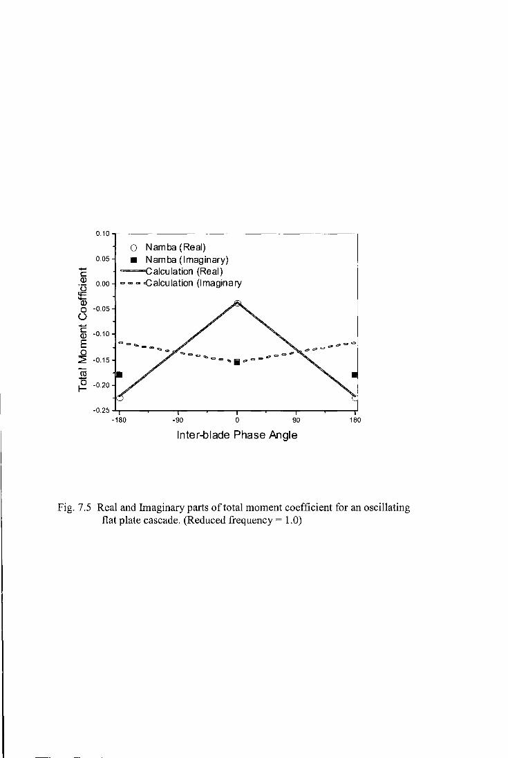
0.10

0 Namba (Real) 0.05 • Namba (Imaginary) - ~alculation (Real) c

Q) 0.00 """""".Calculation (Imaginary '(3

tt= Q5 0 -0.05 0 -c -0.10 Q)

E c;a~~::t't2tca- d'~~e!S

0 ~ -0.15 Cle:tllb.f?coEI

ro ~ -0.20

-0.25 -180 -90 0 90 180

Inter-blade Phase Angle

Fig. 7.5 Real and Imaginary parts of total moment coefficient for an oscillating flat plate cascade. (Reduced frequency= 1.0)

Fig. 7 .6a Controlled diffusion airfoil blade of the oscillating compressor cascade

Ftg. 7.6b Stde view and blade-to-blade view of the computational mesh

Span=20% Span=50% 05 05 • Experiment • Experiment

---calculation Pressure surface ---Galcul ation Pressure surface

00 00

~ ~ :i:l :i:l ~ ~ 8 .()5

8 .()5

~ ~ :::l :::l (/) (/)

~ (/) ·1 0 ~ -1.0 a. a.

-1.5 -1 5

00 02 0.4 06 0 6 1 0 00 02 04 06 0.6 1 0

XIC X/C

Sp;~n=70% Span=OO% 05 05 • Experiment • Experiment

--calculation Pressure surface -calculation Pressure surface

00 00 c c Ql Ql ·o :~ IE ~ 2! .()5 8 .()5 (.)

~ ~ :::l :::l (/) (/)

~ -1 0 ~ -10 a. a.

-15 -1 5

00 02 04 06 06 1 0 00 02 04 oe 08 1 0

XIC XIC

Fig. 7.7 Comparison ofblade surface pressure distribution for steady flow at different spanwise locations for oscillating linear compressor cascade.

Q) 4

~ c. 3

~

0.0

360

270

180

Q) 90 !/)

Cll

a:

-90

-180

0.0

Suction surface IBPA=90 deg

Iii 6.0%C,20%Span ....... 3.3% C, 20% Span

19 6.0% C, 50% Span --- 3.3% C, 50% Span

1>. 6.0% C, 70% Span • • •3.3% C, 70% Span * 6.0% C, 90% span

--3.3%C, 90% Span

02 04 0.6

XJC

06

Suction surface IBPA=90 deg

02

li 6.0% C, 20% Span -- -3.3% C, 20% span

8 6.0% C. 50% Span •••••• 3.3% C. 50% Span

" 6.0% C, 70% Span • • 3.3% C, 70% Span

* 6.0% C, 90% Span -:3.3% C, OO%span

0.4

;• .. i:: ... ·· •• • ....

0.6

XJC 0.8

1.0

1.0

Q) !/) Cll

a:

0.0

Pressure surface

El 6.0% C, 20% span •-- 3.3% C, 20% Span

0 6.0% C, 50% Span ···••••3.3% C, 50% Span

ll 6.0% C, 70% Span • • •3.3% C, 70% span * 6.0% C, 90% span

--3.3% C, 90% Span

0.2 0.4 0.6

XJC

Pressure surface

IBPA=90 deg

06 1 0

IBPA=90 deg 360.,----------------------,

270

180

90

-90

a 6.0% c. 20% Span ---3.3% C, 20% Span

• 6.0% c. 50% Span """ 3.3% C, 50% Span

A 6.0% C, 70% Span • • 3.3% C, 70% span

*' 6.0% C. 90% span --<3.3% C. 90% span

-180 +-~~--.--~--.---.----.-~--1 0.0 02 04 08 08 1.0

XJC

Fig. 7.7a Amplitude and phase of unsteady pressure coefficient at two bending amplitudes of 6.0% and 3.3% of chord. (Reduced frequency=0.4)

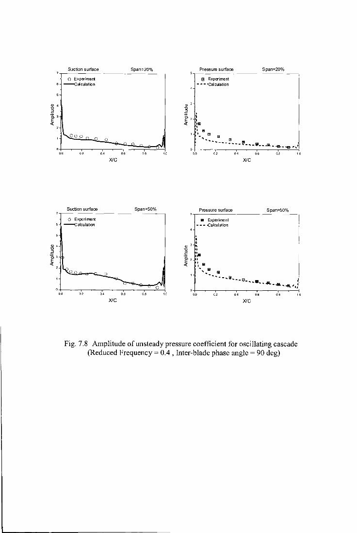
Suction surface

o Experiment 6 -calculation

QJ 4

~ 0.3 ~

QJ 4 "0

~ 15.3

~

0.0

Oo o 0 0

0.2

Suction surface

0 Experiment -calculation

02

Span=20%

0 j 0

0.4 06 06 1.0

XIC

Span=50%

04 0.6 0.6 1.0

XIC

QJ 3

Pressure surface

Iii Experiment ---·Calculation

~ ' a. 2 I

~ ~Iii I I EJ

1 I

0.0 02

Pressure surface

1!1 Experiment ---<Calculation

00 02

Span=20%

0.4 0.6 0.8 1 0

X/C

Span=50%

0.4 06 08 1.0

X/C

Fig. 7.8 Amplitude of unsteady pressure coefficient for oscillating cascade (Reduced Frequency= 0.4 , Inter-blade phase angle = 90 deg)

<1> 4

~ (iJ

~

Suction surface

0 Experiment --calculation

0.2

Suction surface

0 Experiment --calculation

02

04

XJC

04

XJC

Span=70%

0.6 0.8 1.0

Span=90%

0.6 0.6 1.0

Pressure surface

1!1 Experiment : --- <:alculation

' I ' I ·:~~~

\ I \ • Iii)

\' 1!1 ' .... ffi

.. -... ~--

0.0 0.2

Pressure surface

,, Ill Experiment 1 --- <:alculation

4 I 'I II

I I

Q) 3 :

~ ~ 12 'e~

04

Span=70%

--s-- ......... c .. -19 ... - fl...,·.:

I

06 0.6 1 0

XJC

Span=90%

... R- ... - .. ...... --m. ..... <o§.

- ... s, .. ~ ....... '"". " ,.,

of-~---.--~-.--~--~--~-.--~~ 0.0 0.2 0.4 06 0.8 1.0

XJC

Fig. 7.9 Amplitude of unsteady pressure coefficient for oscillating cascade (Reduced Frequency= 0.4 , Inter-blade phase angle = 90 deg)

0.> (/)

"' i£

0.> (/)

"' i£

Suction surface Span=20% ~0,----------------------------------

o Experiment 210 ---calculation

180

90

0

-90

-180 0.0 02

Suction surface 360

0 Experiment

270 -calculation

180

90

-90

-180 0.0 0.2

0

0.4 06 0.6 1.0

XIC

Span=50%

04 06 0.8 1.0

XIC

Pressure surface Span=20% ~0~---------------------------------

Iii Experiment

270 - - - .C aJ cui a lion

180

0.> 90 gJ i£

I

I ,.1 1

l!l 1i! 1!1 Iii D ~~ ol o : sliil ~--lil----~-,-----. ------- .,

\ , . -90 ('

-180 +---~-,---~--.--~---,---~----,.--~----j 00 02 0.4 06 08 1.0

XIC

Pressure surface Span=50% ~0~----------------------~--------,

11 Experiment

270 --- -<:alculation

180

~ 90

i£

-90

-180 +---~--.---~--.--~----.--~--.---~----1 0.0 02 0.4 0.6 08 1.0

XIC

Fig. 7.10 Phase of unsteady pressure coefficient for oscillating cascade (Reduced Frequency = 0.4 , Inter-blade phase angle = 90 deg)

Q) (/) ro It

Q) (/) ro II:

Suction surface 360

Span=70%

0 Experiment 270 --calculation

180

90

0 0

0

-90

-180

00 02 0.4 0.6 0.8 1 0

X/C

Suction surface Span=90% 360~-------------------,

0 Experiment

270 --calculatioo

180

90

-90

-180 00 02 0.4 06 08 1.0

XIC

Pressure surface Span=70% ~Or------------------,

270

180

o Experiment --- .Calculatioo

~ 90 I ~I Ill ro

It fi] g ~ ... o &iJ ca _________ !!1---B~------~ ...... o_, ~ ,,,.- .

I -90

00 02 0.4 06 0.8 1.0

XIC

Pressure surface Span=90% ~Or------------------,

!I Experiment

270 --- <:aiculation

180

. I

~ 90

It 0 1!1 1!1 Iii li Iii 1!1 il li ·::

-90

,~ .... ---------, .... -----------~--'., , II I It

00 0.2 0.4

XIC

06 0.8

~ ~ I

1.0

Fig. 7.11 Phase of unsteady pressure coefficient for oscillating cascade (Reduced Frequency= 0.4 , Inter-blade phase angle = 90 deg)

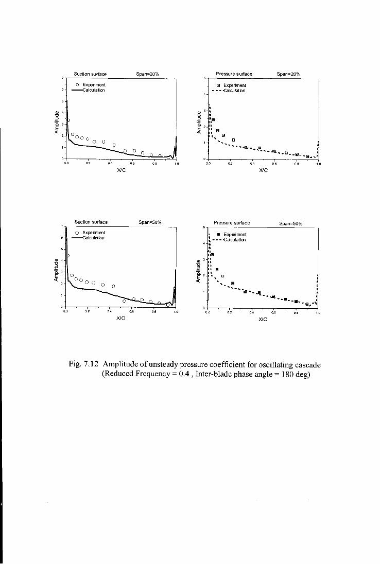
Q) 4 1:l .2 O.a ~

Q) 4 1:l .2 O.a ~

0.0

0.0

Suction surface

o Experiment --calculation

02 04

Suction surface

0 Experiment --calculation

0.2 0.4

XJC

XJC

Span=20%

0.6 O.B 1 0

Span=50%

0.6 08 1.0

Pressure surface

. Q

1!!1 Experiment - --.calculation

Q) 3 '

~ 1~ 0.2

~

DO 02

Pressure surface

• Iii Experiment : --- <:alculation

4 --,, ool!l I \

II II 1!1 II

• ' 13

',, B

04

Span=20%

0.6 08 1 0

XJC

Span=50%

... .,. - ... • I li"'.,...,S I .............. .

...... 1!1 •• 11 I ·-e,•'o

DO 0.2 0.4 0.6 0.8 1.0

XIC

Fig. 7.12 Amplitude of unsteady pressure coefficient for oscillating cascade (Reduced Frequency= 0.4 , Inter-blade phase angle = 180 deg)

Q) 4

~ Q.J

~

Q) 4 "0 .a 0.3 ~

00

0.0

Suction surface

o Experiment --calculation

0.2

Suction surface

o Experiment -calculation

02

0.4

XJC

04

XJC

Span=70%

0.6 O.B

Span=90%

06 0.8

1.0

1.0

Q) 3 "0 .a ~2

Pres sure surface

: • Experiment ~ ---"Calculation . I.

II I I I I Ill ·,, !;I

'~ ......

Span=70%

~~

.; ~~oil ~~ ....

00 0.2 04

Pressure surface

:: • Experiment •' --- ~alculation •' .. ,. •)I

I

'\I 'Iii

~ ~~-. ~

0.6

XJC

... ... ii • ... - 1!1-. -- .. , .. . .

OB 1.0

Span=90%

~ .. • ~--~~ I ... _ .

00 02 04

XJC 06

... ,..~ ,.,.: "''!t, II

08 1.0

Fig. 7.13 Amplitude of unsteady pressure coefficient for oscillating cascade (Reduced Frequency= 0.4 , Inter-blade phase angle = 180 deg)

Suction surface Span=20% MOy-----------------------------------,

o Experiment

270 --calculation

180

Pres sure surface Span=20% ~0.-----------------------------------,

11 Experiment

270 ----calculation

180

~ 90 Jo._o_o_o_o_o __ o __ o _ _,:;o~-0-~0:_o __ o_..)1 90 I• ~· ,u

I Ill

0 : • I::

QJ (/)

"' fi:

-90

-180 -+--~-.--~---.---~--.--~~-.--~--1 00 02 0.4 06 0.8 1.0

XIC

Suction surface Span=50% 360

0 Experiment

270 --calculation

180

90 0 0 0

-90

-180

00 0.2 04 06 08 1.0

XIC

.•• !1--•-------lii!.--Jil--111--1--•-. -90 .--- :

-180 -+---~-.--~---.---~--.-~~-.--~--! 0.0 02 04 0.6 09 1.0

XIC

Pres sure surface Span=50% ~0.---------------------------~------.

• Experiment 270 ---<Calculation

180

90 I \ ••• ,,, ••• o ' II I tl

: •.JL Jt. ---•---•--•--.a.. •-'•' .... - -.- ~ -90 , ,

: -180 -+---~-,--~---.--~--.-~~-.--~--1

0.0 0.2 0 4 06 0.8 '0 XIC

Fig. 7.14 Phase of unsteady pressure coefficient for oscillating cascade (Reduced Frequency= 0.4 , Inter-blade phase angle = 180 deg)

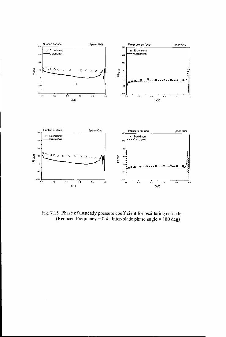
Ql

"' co &.

Ql

"' co &.

Suction surface Span=70% 360

0 Experiment

270 -calculation

160

90

-90 0

-180

00 02 04 06 0.6 1.0

XJC

Suction surface Span=90% 360

0 Experiment

270 ---calculation

160

90 0 0 0

-90

-180

Ql

"' co &.

Pressure surface Span=70% 360,--------------------,

• Experiment

270 ----calculation

160

90

I

• "' ,,, ,,,

0 I IU

: ..... _.!1~--'!--~·-. -·~-·--...__ .... , :: ~ u,

-90 ( I

• ' -160 +--~--.-~---.-~-,--~--.---.-j

0.0 0.2 0.4 06 06 1.0

XJC

Pressure surface Span=90% ~0.--------------~-----

• Experiment

270 ----calculation

180

90 l ,., ,., I •:•

0 I 1 11 ·- .... _ ... __ . ___ ._. _. __ ... _..__ .... ,, •' ,,_ ,. ~: r

-160 0.0 0.2 04 06 0.6 1.0 00 0.2 0.4 06 06 '0

XJC XJC

Fig. 7.15 Phase of unsteady pressure coefficient for oscillating cascade (Reduced Frequency = 0.4 , Inter-blade phase angle = 180 deg)

Suction surface

o Experiment 6 --calculation

<ll 4

~ (iJ

~

<ll 4 "0 2 0.3 ~

00

0.0

0.2

Suction surface

0 Experiment --Galculation

0.2

Span=20%

0.4 06 0.6 1.0

X/C

Span=50%

0.4 06 0.6 1.0

X/C

Pressure surface

Iii Experiment - • -<Calculation

I I I ~ I

II I I.

II

·'..til '... .

Span=20%

"'·- ... ---.---.li-~,Jil.. '

., ,8 • .II • .,. • • I

00 0.2

Pressure surface

• Experiment l ----calculation

~

0.0 0.2

04

04

O.B OB 1.0

X/C

Span=50%

0.6 0.8 1.0

X/C

Fig. 7.16 Amplitude of unsteady pressure coefficient for oscillating cascade (Reduced Frequency = 0.4 , Inter-blade phase angle = -90 deg)

Ql 4

2 0.3 ~

00

Ql 4 1:> .a 0.3 ~

00

Suction surface

0 Experiment ---calculation

0.2

Suction surface

0 Experiment ---calculation

0.2

0.4

XJC

04

XJC

Span=70%

06 0.8 1.0

Span=90%

Ql 3 1:>

~ f2

06 08 1 0

Pressure surface Span=70%

0.0 0.2 04 06 08 1 0

XJC

Pressure surface Span=90%

- !!! Experiment " " ---"Calculation " ' •• ' ' ' ' ' ~-~

\ ~

Iii'---- ..... II

ill Ill• ~ ·~~- -~--.. .;

'Iii,.,

00 0.2 04 06 08 1.0

XJC

Fig. 7.17 Amplitude of unsteady pressure coefficient for oscillating cascade (Reduced Frequency= 0.4 , Inter-blade phase angle = -90 deg)

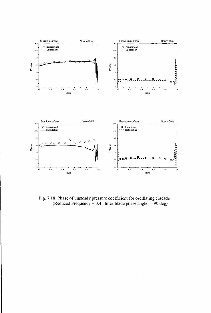
()) (/) ro ~

()) (/) ro ~

Suction surface 360

0 Experiment

270 --calculation

180

~ r.

Span=20%

" 0

Pressure surface Span=20% 360,---------------------,

El Experiment 270 - - -.calculation

180

n n

90~ "

-90

-180

360

270

180

90

-90

-180

0.0 0.2 04 06 0.6 1.0

XJC XJC

Suction surface Span=50% Pressure surface Span= 50% 360

0 Experiment • Experiment --calculation 270

---'Calculation

180 0

0 0 ooO o 0 0 0 0

0 0 I ())

90 'I (/) ro II

_r: I I" a. I I" 0 I Ill . . ..

I • II Ill -90

I'=J!l..lii-A~----~ ---1!1---e--"EE-- '" • "a.l ~

' ' -180 I

0.0 02 04 06 0.6 1.0 0.0 02 0.4 06 0.8 1 0

XJC XJC

Fig. 7.18 Phase of unsteady pressure coefficient for oscillating cascade (Reduced Frequency= 0.4 , Inter-blade phase angle = -90 deg)

Q) U) co a:

Suction surf ace Span=70% 360-,---------------------,

0 Experiment

270 --calculation

180

-90

-180

00 02

Suction surface 360

0 Experiment

270 ---calculation

180

000 0 0 0 90

-90

-180

00 0.2

0

0

0 0 0 0 0 0 _ _)

0

0.4 06 0.8 1.0

XJC

Span=90%

0 0 0

0.4 0.6 0.8 1.0

X/C

Q) U) co a:

Q) U) co .r:: 0..

Pressure surface Span=70% 360,---------------------,

11 Experiment ---.Calculation

270

180

90

-90

-180

300

270

180

90

-90

-180

I I II Ill Ill

I Ill I ltl

:.all~- JL- _Ill_--·- -'1!1. -·- - ... - .... : :: I II

' l 00 0.2 0.4 0.6 06 1 0

XJC

Pressure surface Span=90%

• Experiment ---.Calculation

J ,I, II .~ I

I I

: ··-·. ___ . __ ..... -- ... ·-- ............ _....,,• I I

00 02 0.4 06 08 1.0

XJC

Fig. 7.19 Phase of unsteady pressure coefficient for oscillating cascade (Reduced Frequency= 0.4 , Inter-blade phase angle = -90 deg)

7

...... • Experiment c ... Calculation Q) 6 (.)

li=

di 8 5

0> ,!;;;;; 4 c. E J • co 3 II 0 (.)

.E 2

co • 5-1

'8 • .....

~ 0 -180 -90 0 90 180

Inter-blade Phase Angle

Fig. 7.20 Aerodynamic damping coefficient in dependence of inter-blade phase angle (Reduced frequency= 0.4)

7

...... • Experiment c .... Calculation Q) 6 '(3 li= '+-Q) 5

8 0> • .!;;;;; 4 c. • E co 3 0 • (.)

E 2 co 5-1

"8 • .....

~ 0 -180 -90 0 90 180

Inter-blade Phase Angle

Fig. 7.21 Aerodynamic damping coefficient in dependence of inter-blade phase angle (Reduced frequency= 0.6)