Utah State University Utah State University

DigitalCommons@USU DigitalCommons@USU

All U.S. Government Documents (Utah Regional Depository)

U.S. Government Documents (Utah Regional Depository)

1996

Dutch Experience in Irrigation Water Management Modelling Dutch Experience in Irrigation Water Management Modelling

B J. van den Broek

Follow this and additional works at: https://digitalcommons.usu.edu/govdocs

Part of the Environmental Indicators and Impact Assessment Commons

Recommended Citation Recommended Citation van den Broek, B J., "Dutch Experience in Irrigation Water Management Modelling" (1996). All U.S. Government Documents (Utah Regional Depository). Paper 498. https://digitalcommons.usu.edu/govdocs/498

This Report is brought to you for free and open access by the U.S. Government Documents (Utah Regional Depository) at DigitalCommons@USU. It has been accepted for inclusion in All U.S. Government Documents (Utah Regional Depository) by an authorized administrator of DigitalCommons@USU. For more information, please contact digitalcommons@usu.edu.

1111111111111111111111111111111

PB97-160808 Information is our business.

DUTCH EXPERIENCE IN IRRIGATION WATER MANAGEMENT MODELLING

WINAND STARING CENTRE FOR INTEGRATED LAND, SOIL AND WATER RESEARCH, WAGENINGEN (NETHERLANDS)

1996

u.s. DEPARTMENT OF COMMERCE National Technical Information Service

.... .c Dutch experience in c: u Q) ~

E fa irrigation water Q) .... "" "-

fa Q) management modelling c- o::: Q) ~

1111111111111111111111111111111 0 Q) ...., .!: fa PB97-160808 u 3: B.J, van den Broek (Editor) "-fa "C Q) III C Q) fa

0:::

'-.. --' .- ..

'--- -... l~· .. i,.

. ... :. REPORT 123 REPRODUCED BV: KDa

u.s. o.p.tment ofCOftV1"WC.

Wageningen (The Netherlands), 1996 NItionIII Technic .. hfon'Nltion 1erYk:. Ij>mgtIoId, VIrgInIa 22111

,a •.•

r.

"'J

BIBLIOGRAPHIC INFORMATION

Report Nos:

Title: Dutch Experience in Irrigation Water Management Modelling.

Date: c1996

Authors: B. J. van den Broek.

PB97-160808

Performing Organization: Winand Staring Centre for Integrated Land, Soil and Water Research, wagenlngen (Netherlands). Agricultural Research Dept.

Supplemental Notes: Details in illustrations may not be fully legible in microfiche. Also pub. as Wlnand Staring Centre for Integrated Land, Soil and Water Research, Wageningen (Netherlands). Agricultural Research Dept. rept. no. REPT-123.

NTIS Field/Group Codes: 98C (Agricultural Equipment, Facilities, & Operations)

Price: PC A08/MF A02

Availability: This product may be ordered from NTIS by phone at (703)487-4650; by fax at (703)321-8547; and by email at 'orders@ntis.fedworld.gov'. NTIS is located at 5285 Port Royal Road, Springfield, VA, 22161, USA.

Number of Pages: 133p

Keywords: *Netherlands, *Irrigation water, *Mathematical models, *Drainage systems, Irrlgatlon systems, Decision support systems, Ground water, Hydrology, Irrigation practices, Irrigation effects, Drainage effects, Water management(Applied), Water allocation(Policy), SOil-water-plant relationships, Hydrodynamics, Water delivery, Agriculture, Computerized simulation, Meetings, *Foreign technology.

Abstract: Contents: Modeling the sOil-water-crop atmosphere system to improve agrlcultural water management in arid zones (SWATRE); Groundwater approach to drainage design in irrigated agriculture (SGMP); Computer Rrogram for flume and weir design (FLUME 3.0); A hydrodynamic model in the design of operational controllers for water systems (MODIS/MATLAB); Decision support simulation model for water managemnet at a regional and national scale (SIWARE); Management of water delivery systems (RIBASIM/OMIS); A water allocation, scheduling, and monitoring program (WASAM); and Irrigation agencies, farmers and computational decision support tools.

III 1111111111111111111111111111 PB97-160808

Dutch experience in irrigation water management modelling

B.J. van den Broek (Editor)

Report 123

DLO Winand Staring Centre, Wageningen (The Netherlands), 1996

Abstract

Van den Broek, B.J. (ed.), 1996. Dutch experience in irrigation water management modelling. Wageningen, DLO Winand Staring Centre for Integrated Land, Soil and Water Research. Report 123. 132 pp.; 43 figures; 16 tables; 2 photographs; 130 references.

The first workshop organized by the National Committee ofthe Netherlands ofthe International Commission on Irrigation and Drainage (ICID) has brought many Dutch scientists together in the field of irrigation water management to exchange their experiences in modelling. The models range from rather complex, one-dimensional simulations to large-scale irrigation, drainage and salinity projects in all parts of the world.

Keywords: decision-support system, drainage, groundwater, hydrology, irrigation, models

ISSN 0927-4537

NTIS is aUlhorized to reproduce and sell this report. Permission for turther reproduction must be obtained from the copyright owner.

©1996 DLO Winand Staring Centre for Integrated Land, Soil and Water Research (SC-DLO) P.O. Box 125, NL-6700 AC Wageningen (The Netherlands) Phone: 31 (317) 474200; fax: 31 (317) 424812; e-mail: postkamer@sc.dlo.nl

No part of this publication may be reproduced or published in any form or by any means, or stored in a data base or retrieval system, without the written permission of the DLO Winand Staring Centre.

The DLO Win and Staring Centre assumes no liability for any losses resulting from the use of this report.

Project 60021 [Rep123.HM/08.96]

Dutch experience in irrigation water management modelling

Contents

page

Preface 11

1 Modelling the soil-water-crop-atmosphere system to improve agricultural water management in arid zones (SW ATRE) 13 W.G.M. Bastiaanssen, 1. Huygen, 1.K. Schakel and B.J. van den Broek Introduction 13 Schematization of the SW A TRE model 14 Examples of SW A TRE applications 17 Calibration of model parameters 18 Results with local SW A TRE simulations 19 Regionalization of local SW A TRE results in Haryana, India 24 Conclusions 26 References 27

2 Groundwater approach to drainage design in irrigated agriculture (SGMP) 31 1. Boonstra, Sultan A. Rizvi and M.N. Bhutta Introduction 31 Nodal net recharge by inverse modelling 33 Decomposition approach 35 Design nodal net recharge 37 Considerations on drainable surplus 39 Discussion of results 41 Acknowledgements 44 References 45

3 Computer program for flume and weir design* (FLUME 3.0) 47 A.J. Clemmens, M.G. Bos, 1.M. Groenestein and 1.A. Replogle Introduction 47 Theory 47 Design requirements 48 Design evaluation 52 Databases, data entry and output 54 References 56

4 A hydrodynamic model in the design of operational controllers for water systems (MODISIMATLAB) 57 M.G.F. Werner, 1. Schuurmans, H.J. Campfens and R. Brouwer Introduction 57 The hydrodynamic model: MODIS 58 The mathematical package: MATLAB 58

Combination of MODIS and MATLAB 59 Model application: Punggur Utara, Indonesia 60 Model application: River Maas, the Netherlands 64 Discussion and conclusions 66 References 66

5 Decision support simulation model for water management at a regional and national scale (SIW ARE) 69 D. Boels Introduction 69 Model description 69 Modules of SIW ARE 70 Schematization, input data and output 74 Calibration and validation 76 Model applications and capabilities 80 Crop response to water management 82 References 85

6 Management of water delivery systems (RIBASIMIOMIS) 87 W. Schuurmans and G. Pichel Introduction 87 Selection of appropriate model 87 Hydraulic versus reservoir model 87 The model RIBASIM 88 The model OMIS 92 Example case: Anambe catchment area, Senegal 95 Example case: Fayoum scheme, Egypt 99 Observations 101 References 102

7 A water allocation, scheduling and monitoring program (WASAM) 103 A.J. van Achthoven and l.F. C. de long Introduction 103 Organizational framework 104 Outline of the WASAM program 108 Field water management 111 Preconditions for using the WASAM approach 112 Results and conclusions 114 References 115

8 Irrigation agencies, farmers and computational decision support tools 117 M. Menenti and c.A. van den Hoven Introduction 117 Decision support tools 119 Irrigation water management: regional and on-farm 122

Optimization methods, monitoring performance and administrative ~es 1~

Missing elements and research needs 129 References 130

Tables 1.1 A limited selection of SW A TRE applications 17 1.2 Categorized input data necessary to operate SW A TRE 18 1.3 Soil-water and crop water relationships which are to a certain extend uncertain

and have to be locally calibrated 19 1.4 Accuracy of SW A TRE simulations expressed as a Root Mean Square Error

(RMSE) between model prediction and field measurement in an irrigated vineyard (Mendoza, Argentina) with respect to soil water content, e, and solute concentration, C, for depth intervals of 25 cm 20

1.5 Cumulative simulated soil water balance terms (cm) from sowing to harvest for different crops 22

1.6 Simulated cumulative salt balance (mg/cm2) during 365 days for canal water (CW) and drainage water (DW) field experiments 24

1.7 Water management scenarios for land reclamation in Haryana 24 2.1 Synthetical design monsoon nodal net recharge values. 38 4.1 Performance parameters for simulated case for the whole month of

January 64 5.1 Pre-set model accuracy criteria: average monthly deviation allowed 78 5.2 Ratio of crop yield reduction (% )/evapotranspiration reduction (%) and the

threshold value for evapotranspiration reduction (%), above which this ratio is valid for the major field crops 84

5.3 SIW ARE development team 84 7.1 The required number of field staff 112 8.1 Overview of legislation and administrative regulations determining water

allocation in Mendoza, Argentina 120 8.2 Irrigation application strategies 125 8.3 Definition of irrigation performance indices; for each index the required land

use data are indicated explicitly, with their source; the models necessary to calculate each index and the ancillary data 127

Figures 1.1 Artists impression of an irrigation scheme emphasizing the role of on-farm

water management in establishing efficient irrigation water use 14 1.2 Moisture and solute flow directions in a SW A TRE-column 15 1.3 Measured and simulated soil water storage in a 125 cm thick rootzone of

a Mendozian vineyard 20 1.4 Modelled and observed soil water storage for the Sirsa experiment 22 1.5 Simulated and in-situ measurements of water table at the reuse of drainage

water experiment under shallow water table conditions, Hisar India 23 1.6 Relative transpiration calculated with SW ATRE for different geographical

units according to the water management scenarios listed in Table 1.7 25

2.1 Schedule I-B area showing the location of the eleven sump units 32 2.2 Nodal network map for Schedule I-B area 34 2.3 Comparison of seasonal average areal net recharges based on the

decomposition approach and on the inverse modelling result 37 2.4 Representation in SGMP of the areas in need of drainage in S-I-B area

according to original USBR design 42 2.5 Areas in need of drainage in S-I-B area according to SGMP with an average

permissible depth-to-watertable of 1.5 m 43 3.1 The user can choose from seven shapes for the approach and tail water

channels. For the control section, fourteen shapes are available 51 3.2 Example of a design report given by FLUME 3.0 53 3.3 Graphical data entry screen 55 4.1 Program structure of combination MODIS and MATLAB 59 4.2 Layout of water system used in case study 61 4.3 Discharge simulation results for a 10 day period 63 4.4 River Maas, with location of weirs 65 5.1 Flow chart of the SIW ARE model, its submodels and input and output 71 5.2 Example of soil salinity distribution before and after rice growing

season 73 5.3 Subdivision of the Nile Delta of Egypt into calculation units for SIWARE

application 75 5.4 Model deviation on single catchment scale for the Delta Regions East,

Middle and West of Egypt. 79 5.5 Relation between relative crop yield decrease and relative evapotranspiration

reduction 83 6.1 Example schematization of a river basin in Morocco. On the left the real

life system, and on the right the schematized system in RIBAS 1M. 90 6.2 Example of the RIBASIM interface, showing a GIS map of Upper Egypt

with the RIBASIM-network and the 'node selection menu' 91 6.3 Basic simulation approach. 93 6.4 OM IS is used as a decision support model for the irrigation manager 94 6.5 Crop pattern diagram and associated water balance using OMIS 94 6.6 Data flows to and information flows from a water operation centre 95 6.7 Screen image of OMIS, showing the drought stress for time step 10 in the

Cidurian scheme, Indonesia. 96 6.8 Schematization of two alternatives of the Anamb(YKayanga system in

RIBASIM 98 6.9 Map of the Fayoum irrigation scheme (top) and OMIS model

schematization 100 7.1 Information flow 104 7.2 Typical project organization structure 106 7.3 Schematic layout of an irrigation system 107 7.4 Water Allocation Scheduling And Monitoring (WASAM): an overview 108 7.5 Time chart of W ASAM 110 7.6 Monitoring graph - Kinda weir releases - wet season 1987 111 7.7 Information flow and tasks of the field staff and farmers 113 8.1 Conceptual scheme of functional constraints affecting the flexibility of on-

farm irrigation strategy in response to the market environment 119 8.2 Values of marginal benefit of total water supply for four different irrigation

strategies; results obtained with the simulation model SIMGRO 123

8.3 Average utility values per feature for an average year 126 8.4 Change in irrigated area by tertiary unit 129

Photographs 3 .1 FLUME 3.0 calculates a rating table based upon as-built dimensions 49 3.2 The addition of a sill to the bottom of the canal creates a low-cost and

accurate flow-measuring device 52

Preface

On march 31 1995 the National Committee of the Netherlands of the International Commission on Irrigation and Drainage (ICID) organised the first national workshop entitled 'Use of simulation models in irrigation water management'.

In the last decades, a vast amount of models has appeared in the field of water management at large. These models often range in complexity and are applied in numerous types of studies. Many of these models have appeared from the hands of Dutch scientists or in cooperation with others abroad and used in research projects across the globe.

The main aim of this first national workshop was to exchange existing know-how and experience in the broadest sense of irrigation water management modelling. A second aim was to further enhance the scientific ties for better cooperation in national projects and even more so on the international platform. The models presented range from small scale research studies in the Rhine river basin to large scale projects in the inland valleys of south east Asia.

During this workshop eight papers were presented by Dutch researchers representing the International Institute for Land Reclamation and Improvement (Wageningen), Delft University of Technology (Delft), HASKONING, Royal Dutch Consulting Engineers and Architects (Nijmegen), Delft Hydraulics (Delft), DHV -Consultants (Amersfoort), Euroconsult BV (Arnhem) and DLO-Winand Staring Centre for Integrated Land, Soil and Water Research (Wageningen). The presentations held during this workshop have been adapted for publication in this issue for which we are thankful to the authors.

Preceding page blank 11

1 Modelling the soil-water-crop-atmosphere system to improve agricultural water management in arid zones (SWATRE)

W.G.M. Bastiaanssen, J. Huygen, J.K. SchakeI and B.J. van den Broek

DLO Winand Staring Centre for Integrated Land, Soil and Water Research, P.O. Box /25, 6700 AC Wageningen, the Netherlands.

Introduction

Irrigation aims at enhancing biomass production through an increased crop water use. Waterlogging and salinization should be prevented and/or combatted by accurately providing the amount of water needed for crop growth and salt leaching. The success of sustainable water management system lies essentially in adapting the irrigation and drainage techniques such that the annual changes in water and salt content are negligibly small. The irrigation water supply should be such that crop evaporation is not hindered by a shortage of water. Percolating soil moisture conveys soluble salts by advection downward which leaches the rootzone but may create at the same time adverse effects by pushing the water table upward. Sub-surface drainage systems discharge excessive soil moisture and should prevent the rootzone from moisture saturation and unacceptable high salinity levels. Lateral drains convey the effluent from the field to a collector. In absence of a drainage infrastructure, the irrigation water supply should be adapted such that most water from irrigation and rainfall will evaporate by crop and soil.

From an academic viewpoint, the desired amount of water at required at the farm-level can be calculated on a day-to-day basis considering a certain probability of rainfall, initial field wetness, initial soil salinity, given evaporative demand of the atmosphere and crop properties. An operational procedure for such a sophisticated system can be implemented only if an on-demand water distribution systems is present. For rotational systems, the moments of water delivery and the depth of application depend strongly on water management policies followed.

Farm-economic aspects of beneficiaries can have an overriding importance on the desired local water management, i.e. the financial possibility to construct sub-surface drainage systems, the purchase of diesel pump to lift surface water from the irrigation and/or drainage canal or the use of small tubewells for extracting groundwater. The expected prices of the products have immediate effects on the financial possibilities to purchase water rights, water volumes and durable equipment. In many countries, the availability of labour for irrigation is another constraint for adequate on-farm water management.

Preceding page blank 13

Occasionally, water delivery is in accordance to what is locally desired, but the overall efficiency of irrigation is disappointingly low (Wolters, 1992). Since large irrigation schemes may show considerable variability in soils, crops, elevation and hydrology, the water demand at (sub-) scheme level is much more complex to estimate than at farm level. Nevertheless, we believe that on-farm water management should be the cornerstone on which regional water management is based (Figure 1.1). The latter implies that regionalization of on-farm water management strategies should rely on regional geographical information on soil type, crop type, salinity, water table etc.

"..lUU-"urface drainage

SWATRE - column

River

Fig. 1.1 Artists impression of an irrigation scheme emphasizing the role of on-farm water management in establishing efficient irrigation water use

The effects of on-farm water management for physically different conditions can be analyzed with numerical simulation models, either when a technical or a social irrigation and drainage scenario is considered (Menenti, 1994). These models provide the opportunity to study the response of crop yield, soil salinity and soil moisture conditions to an imposed water management scenario. The impact of interventions in water management by different timings, application depths, water qualities, drain depth and drain spacing can be studied in this manner. The current paper addresses how the SWATRE @.oil Water Actual TRanspiration Exentend) model has been used for this purpose, which data should be available and shows examples on the attainable accuracy.

Schematization of the SW A TRE model

SW A TRE is a mechanistic, deterministic model for simulation of one-dimensional unsaturated-saturated soil water flow (Feddes et aI., 1978; Belmans et aI., 1983).

14

Recently, SWATRE has been extended with a module which describes solute and pesticide transport (Work Group SWAP, 1994). Soil moisture transfer is computed with the Richard's equation (Richards, 1931). The soil therefore has to be described in terms of soil hydraulic properties, i.e. water retention and hydraulic conductivity, respectively a hm( e) relationship and a k(hm) relationship. The soil hydraulic properties may be specified by means of the Van Genuchten analytical functions (Van Genuchten, 1980). The movement of solutes is computed by the mechanisms of convection, dispersion, adsorption, decay and lateral drainage. Continuity of soil water content and solutes is ensured by separated continuity equations for both entities. A sink-term describes the extraction of soil moisture by roots as a function of matric pressure and osmotic pressure head. The rootzone is divided in sub-layers which enables a variable water uptake pattern (Figure 1.2).

,1/ -0-/1'

93 • C3

94 • C4

9s • C5

9j • Cj

9j . Cj

9n · Cn

Q

Fig. 1.2 Moisture and solute flow directions in a SWATRE-column

A sink-term of water uptake by roots needs to be prescribed according to the drought and salt tolerance of the crop in question. The drainage component of the SW A TRE model is based upon the Hooghoudt and Ernst equations (Ritsema, 1994) selection being dependent on the hydraulic resistance of the various soil layers in the heterogeneous soil profile. At the lower boundary, either pressure head, soil water

15

content, free drainage, known flux or a known flux-water table relationship can be specified. The maximum crop and soil evaporation can be determined by various options (Penman, 1948; Makkink, 1957; Monteith, 1965; Priestley and Taylor, 1972). For a more thorough understanding on the formulation and flow mechanisms dealt with in SWATRE, one is kindly referred to Feddes et al. (1978), Belmans et al. (1983), Feddes et al. (1988), Van Dam et al. (1990) and Van Dam and Feddes (1996).

The interrelation between irrigation, drainage and crop water use appears from the water balance, which for a one-dimensional unsaturated/saturated soil column can be written as:

(1.1)

where: ~ W = water storage change inside the soil column (ranging from the soil surface

to the lower level where Q applies) Q = flux through the bottom of the soil column (positive upward) P = gross precipitation lIT = irrigation water supply Tact = actual crop evaporation rate Eact = actual soil evaporation rate Ei = evaporation of precipitation intercepted by foliage Ew = evaporation of water ponded at the soil surface R = runoff arising from delayed infiltration processes Dr = drainage by an artificial sub-surface drainage system St = ponded layer at the land surface

The net infiltration into the soil, Inf' can be obtained as:

(cm/d) (1.2)

The partitioning between Inf and R is calculated with the Richards equation. Surface runoff is triggered if P + lIT exceed Inf + Ei + Ew + St. Hence, water application techniques should be such that R, Ew, and Ei are kept to a minimum and lIT and Inf

should be approximately equal.

When irrigation water contains solutes, then seepage Q forms a hazardous term for salinization. The salt balance of the soil can then be expressed as:

(1.3)

where ~C is the change in solute concentration inside the soil profile between the soil surface and the depth to which Q applies. The suffix denotes the different solute concentration related to the different water fluxes. Especially when the water table is in the vicinity of the rootzone, capillary rise will convey the salts (Q C3) upwards to the rootzone. For humid climates the aim of a drainage system is to control ~W, whereas for (semi-) arid conditions drainage should keep ~C at a zero level or preferably make it negative for longer time periods. As it is practically and (often)

16

financially impossible to construct drainage systems at small plots, possibilities to adjust the irrigation regime by means of lIT C1 in relation to Q C3 is an alternative solution.

Examples of SW A TRE applications

SW ATRE has proven its versatility and its power in many hydrological studies under a wide variety of climatic conditions and for several agricultural crops. The physical concept of SW A TRE makes the model suitable for irrigation scheduling, drainage design, percolation assessments (i.e. recharge to deep groundwater), rainfall-runoff studies, long term salinization and studying the fate of substances such as solutes, nitrogen and pesticides (see Table 1.1). The tendency of the applications is, without exceptions, directed into research. Operational on-farm water management with SW A TRE is not common. The model output helps however researchers to extract more practical guidelines and look-up tables, as:

- effects of drain spacing on water table fluctuations; - drain depth in relation to amount of reusable drainage effluent; - leaching requirement; - critical leaching periods; - application efficiency in relation to soil type and rooting depth; - specification of field capacity conditions; - capillary rise behaviour; - irrigation interval in relation to crop developing phase.

Table 1.1 A limited selection of SWATRE applications

Source

Boers et al. (1986) Ragab et al. (1990a,b) Feddes and van Wijk (1990) De Jong and Kabat (1990) Boesten and van der Linden (1991) Feddes and Bastiaanssen (1992) Zepp and Belz (1992) Kabat et al. (1992) Clemente et al. (1994) Bastiaanssen et al. (1994) Faria et al. (1994) Huygen et al. (1995) Menenti (1995) Van den Broek and Kabat (1995) Beekma et al. (1995) Van Dam and Feddes (1996)

Country of study

Israel Germany The Netherlands The Netherlands The Netherlands Egypt Germany The Netherlands Canada India Brazil Southern Europa Argentina Scotland Pakistan Pakistan

Application

Water harvesting Crop water consumption Land evaluation Grass production Pesticide leaching and persistence Sprinkler irrigation scheduling Sensitivity study Crop production Intercomparison simulation models Irrigation and drainage Intercomparison simulation models Irrigation scheduling Rainfall runoff Potato production Waterlogging and salinity Irrigation and drainage

17

Calibration of model parameters

The required input data for SW A TRE is large. The data can be categorized into soil, crop, meteorological and hydrological parameters (Table 1.2). The (un) certainty of each individual input parameter depends on its measured accuracy in the field or laboratory. For instance, wind speed can be obtained in a straightforward manner (anemometer) whereas rooting depth is much more cumbersome to obtain because roots are irregularly distributed and maximum root length is not similar to the discretized depth.

Model calibration is often executed in a subjective sense and the parameter set obtained (Table 1.2) is consequently non-unique. The experience of the model user usually determines the calibration philosophy followed. However, a calibration procedure for model parameters as shown in Table 1.2 should be in a structural manner, for instance: - divide a simulation period into different crop growing periods and associated

phenological stages; - assign sensitivity to each of the model parameters; - assign accuracy to each of the model parameters; - fix the model parameters which can be accurately measured; - specify the most likely parameter space on basis of literature or other sources which

cannot be accurately measured; - select shorter simulation periods in which the given parameters are most sensitive; - calibrate these model parameters in sequence of their sensitivity and for the

simulation periods selected; - validate the model parameters for a simulation period in which no calibration has

been realized.

Table 1.2 Categorized input data necessary to operate SWATRE (parameters between brackets are optional)

Soil

Water retention char. Saturated hydraulic condo Unsaturated hydraulic condo Bulk density Dispersion length Salt diffusivity Adsorption coefficient Freundlich coefficient

Crop

Rooting depth Soil coverage Leaf Area Index Drought resistance Salt resistance (Crop height) (Albedo)

Meteo

Solar radiation Air temperature (Air humidity) (Wind speed) (Drain depth) (Drain diameter) (Depth imperm. layer)

Hydrology

8(z)-init. C(z)-init. Bottom bound. (Drain spacing)

Practical experience has learned that soil-water relationships obtained from laboratory measurements are rather uncertain as (i) 'un-disturbed' soil cores can hardly be collected without destructing the soil

matrix of the sample; (ii) the thermal regime in an arid environment encountered in the field deviates

significantly from the conditioned environments in the laboratory; (iii) spatial variations in horizontal and vertical orientation can hardly be sampled

in the field and (iv) hysteresis effects forthcoming from the wetting/drying history are difficult to

realize in the laboratory environment.

18

Crop water relationships change with local crop varieties and their bio-physical adaptations to the local environment and may therefore not a priori be taken from standard look-up tables. Although it goes beyond the scope of this paper to discuss the physical/chemical meaning of parameter uncertainty and their need for calibration, standard values from literature are seldom suitable for predictions of local water and salt balances.

The unknown soil-water and crop-water relationships can be nicely calibrated from information on the temporal behaviour of the local 9(z) and C(z) profiles. As a matter of fact, soil properties can be best calibrated during the fallow period when interferences from crop-water relationships on moisture and solute flow is ruled out. The availability of transient 9(z,t) and C(z,t)-profiles at the appropriate times (at end of water application, at field capacity, before next irrigation, at start of season, at end of season) are extremely useful to obtain the uncertain parameters of Table 1.3.

Table 1.3 Soil-water and crop water relationships which are to a certain extend uncertain and have to be locally calibrated (after Bastiaanssen, 1995)

1. Residual soil water content, e r (Van Genuchten, 1980) 2. Inverse of the matric pressure head at air entry, a (Van Genuchten, 1980) 3. Empirical parameter determining slope of the hm(S) relationship, n (Van Genuchten, 1980) 4. Empirical parameter determining slope of the k(hm) relationship, I (Van Genuchten, 1980) 5. Saturated hydraulic conductivity, ksat of the entire SWATRE-column 6. An-isotropy factor for k/kh' with respect to horizontal flow to the laterals 7. Sink term critical pressure heads, hI to h4 (Feddes et aI., 1978) 8. Salt tolerance factor, £ (Bastiaanssen, 1992) 9. Empirical coefficient for bare soil evaporation, B (Boesten and Stroosnijder, 1986)

10. Effective depth of the rootzone for soil moisture extraction, zr (Feddes et aI., 1978) 11. Fractional contribution of max. crop evaporation across rootzone, Smax(z) (Prasad, 1988) 12. Thickness of top layer in rootzone which does not extract moisture, znon 13. Diffusion coefficient, Ddif (Boesten and van der Linden, 1991) 14. Dispersion length, Ldis (Boesten and van der Linden, 1991) 15. Adsorption coefficient, K (Boesten and van der Linden, 1991) 16. Freundlich coefficient, F (Boesten and van der Linden, 1991) 17. Distance to the impermeable layer, D (Ritsema, 1994)

Results with local SW A TRE simulations

Mendoza, Argentina The province of Mendoza situated at the pediments of the Andes has typical Mediterranean crops such as grapes, olives, fruits and vegetables. Mismanagement by means of excessive irrigation water supply in combination with an inadequate drainage disposal system has created waterlogging at the lowlands. The (semi-) arid climate with a continuous high atmospheric evaporative demand of the atmosphere and the water table in the vicinity of the soil surface has induced secondary salinization. At the Lavalle pilot area near the town of Mendoza, subsurface drainage systems were constructed at different spacings and a leaching experiment was initiated (Mirabile, 1990). SW ATRE was implemented to describe the water and salt fluxes during and after the leaching experiment. The soil-water and crop-water relationships were calibrated with 9(z) and C(z) profiles collected on 15 crucial days according

19

to the afore mentioned procedure on sensitivity and uncertainty. Extraction of soil moisture from the upper 25 em of the soil for the analysis of near surface solute concentration failed because of the high suction present in this part of the soil matrix. First, transient 8(z,t)-pattems were calibrated after which soil salinity parameters were determined from C(z,t). Soil profiles were sampled both at the upstream and the downstream end of the irrigation borders. SWATRE's attainable accuracy can be evaluated by comparing the model predictions with field measurements (Table 1.4).

Table 1.4 Accuracy of SWATRE simulations expressed as a Root Mean Square Error (RMSE) between model prediction and field measurement in an irrigated vineyard (Mendoza, Argentina) with respect to soil water content, e, and solute concentration, C, for depth intervals of 25 cm. The average soil water content and soil salinity is added (after Bastiaanssen, 1995).

Depth RMSE-8 Average-8 RMSE-C Average-C (cm) (cm3/cm3

) (cm3/cm3) (mg/cm3) (mg/cm3)

0- 25 0.045 0.27 25- 50 0.040 0.31 0.49 3.10 50- 75 0.042 0.37 0.54 3.30 75-100 0.044 0.41 0.86 2.96

100-125 0.041 0.45 0.86 2.58

The model was initialized just once while the 15 profiles reflect a complete annual cycle. The relative error (RMSE/average) is approximately 12% for e and 23% for C. These errors reduce substantially if the total rootzone (125 em for vineyard) is considered. Figure 1.3 shows the agreement for the 15 measurements (RMSE=0.024 cm3/cm3

). Measured (em) 54

50

46

42

38

1 : 1

/. •• •••• • • •

•

Modelled (em)

Fig. 1.3 Measured and simulated soil water storage in a 125 cm thick rootzone of a Mendozian vineyard (after Bastiaanssen, 1995)

Integration of these 15 field observations yielded an average value of W=44.5 em while the SWATRE simulations differed only by 2% (W=43.7). Taking the water storage term (W) as rather accurate, the annual water and salt balance at on-farm level are sufficiently understood for water and salinity management purposes if being calibrated with local 8(z) and C(z) profiles.

20

Soil water storage 0 - 50 em depth (em) 20 @ Soil water storage 0 - 50 em depth (em)

20 <ID

15 15

10 10

o o~ °rV\o 0__ ~,....~o~ / -..........; ~ ~v ...... e ••

o 0

5 5

O~--~----~----L---~ ____ ~ __ ~ OL-__ -L ____ L-__ ~ __ ~L_ __ ~ __ ~

300 400 500 600 700 800 900 300 400 500 600 700 800 900 Simulated period (1990 - 1992) Simulated period (1990 - 1992)

Soil water storage 0 - 50 em depth (em) 20 {O

Soil water storage 0 - 50 em depth (em) 20 ~

15 15

10 10

5 5

OL---~--~ __ ~ __ ~ __ -L __ -L __ ~ OL---~--~--~ __ ~ __ -L __ ~ __ ~

200 300 400 500 600 700 800 900 200 300 400 500 600 700 800 900 Simulated period (1990 - 1992) Simulated period (1990 - 1992)

Fig. 1.4 Modelled and observed soil water storage for the Sirsa experiment. Part A: wheat-cotton in the 0-50 cm layer, Part B: wheat-cotton in the 50-100 cm layer, Part C: mustard-fallow in the 0-50 cm layer, Part D: mustard-fallow in the 50-100 cm layer, Sirsa, India (after Singh, 1995).

Table 1.5 Cumulative simulated soil water balance terms (cm) from sowing to harvest for different crops (after Singh, 1995)

Crop P lIT Tact E act Q !!..W Epot Tpot

Wheat-91 4.2 24.0 26.5 5.5 -0.1 -3.8 10.4 33.6 Wheat-92 4.0 28.6 28.4 7.5 -0.3 -3.6 11.0 32.0 Cotton-91 20.5 27.5 37.1 14.7 -0.1 -4.0 31.3 62.5 Mustard-91 4.6 8.7 14.2 8.3 0.0 -9.3 21.7 22.1 Mustard-92 3.2 12.0 13.6 7.9 -0.1 -6.4 19.1 23.2

22

Haryana, India Haryana State is located in the northwestern part of India and the geophysical position (pediment of Himalayas) is quite similar to the location of the Mendoza province in relation to the Andes. More than 65 percent of the state lies in the arid and semi-arid tract with scanty and erratic rainfall. Waterlogging and salinization pose immediate threat to the sustainability of agricultural production and physical environment of Haryana. An annual rise in water table, at an alarming rate between 0.3 to 1 m per year, has been recorded in nearly 75 per cent of its arable land area while the water table has almost reached the surface in 10 percent of the area. Irrigation water losses on the farm have been reported to be one of the major causes of the rise in water table. Different improvements in on-farm water management were studied by means of field trials at the experimental farms of Haryana Agricultural University (Bastiaanssen et aI., 1994) as:

- Abeyance of post-sown irrigation water supply under shallow water table conditions; - Reduced water application at deep water table conditions and; - Reuse of drainage water under shallow water table conditions.

Reduced water application SW ATRE was used during a three year cultivation period with wheat-cotton and mustard-fallow growing cycles at the university farm at Sirsa during 1990-1992 (Singh, 1995). The water table was situated at 15 m depth and as such a free drainage lower boundary option was selected. The model parameters listed in Table 1.2 were calibrated from observed 8(z) profiles collected at regular time intervals during 1990 after which they were kept constant during the validation period (1991 to 1992). The crop water requirements were computed with the Priestley & Taylor approach as air humidity and temperature were (systematically) underestimated and overestimated respectively by the meteorological observations on non-irrigated drylands. Potential evaporation calculated by a Penman-Monteith type expression will then result in unrealistically high values (Kumar and Bastiaanssen, 1993) whereas the Priestley & Taylor method is driven by radiation. Soil salinity did not play an essential role as irrigation canal water was of good quality and secondary salinization was ruled out by the presence of a deep water table. The simulated soil water storage matched quite satisfactory with observed values for the entire simulation period (Figure 1.4), implying a well validated model. The impression exists that the mustard-fallow simulations are slightly more accurate than for wheat-cotton. Although moisture levels changed rapidly between successive irrigation turns, the simulations revealed near identical changes. The water balance presented in Table 1.5 shows that soil moisture was depleted (/1 W is negative). Furthermore, Table 1.5, describing the reduction in Tact compared to Tpot, shows that stress applies to the cotton and mustard crops, (being a logical consequence of water applications being far beyond the crop water requirement).

21

Reuse of drainage water Haryana is marked by an inland drainage basin condition with no natural outlet for drained and/or pumped water. Therefore, drainage effluent needs to be used locally. The possibility of reusing drainage effluent were investigated by the installation of a tile drainage system at a depth of 2.7 m and different spacings at the Hisar farm. The irrigation treatments chosen were (i) pure canal water, CW, (ii) full reuse of drainage water, DW, (iii) canal water in alternation with drainage water, AW and (iv) canal water mixed with drainage water in 1:1 ratio, MW (Kumar, 1995).

A four year data set on water table observations were consulted to calibrate and validate SW ATRE (1989: calibration; 1990-1993: validation). The results are depicted in Figure 1.5. The monsoon effect on water table levels are clearly visible. The average root mean square error between model predictions and field observed water tables turned out to be 18 cm which considering the limitation of a theoretical model, is fairly encouraging.

Depth to water table (m)

-1.5

•• • • •• . -..... . /_-... .-

••• r-- ". ( •• . ; ... ~ .~ ·v· ~. . e. • • .... •• •

-2.0

-2.5

• •

•

• • ••

-3.0 '-------'-----'-----'------'-----'-----'-------' 200 400 600 800 1000 1200 1400 1600

Day number (1 Jan 1989 = day 1)

Fig. 1.5 Simulated and in-situ measurements of water table at the reuse of drainage water experiment under shallow water table conditions, Hisar India (after Kumar, 1995)

The annual salt balance of the two extreme irrigation treatments CW and DW are presented in Table 1.6. The averaged annual value of ~C=25.9 mg/cm2 for CW and 93.6 mg/cm2 for DW reveal that even for CW, a net influx of salts occur (see Equation 1.3, Q C3). For the DW scenario, salinization is even further enhanced by lIT C!. Although reuse of drainage water is an attractive solution to reduce the total disposal of drainage effluent, it is evident that it is a hazardous threat to sustainable agricultural development. Reductions through the A W -treatment is therefore at least a better step in the direction of reducing the required drainage volumes.

23

Table 1.6 Simulated cumulative salt balance (mglcm2) during 365 days for canal water (CW)

and drainage water (DW) field experiments (after Kumar, 1995).

Year Treatment IITC r Q C2 Dr C3 LlC

1990 CW 10.2 40.0 43.3 +6.8 1991 CW 9.8 75.7 52.8 +32.7 1992 CW 10.7 108.9 81.4 +38.2

1990 DW 83.4 40.1 46.7 +76.7 1991 DW 93.3 75.7 58.5 +110.5 1992 DW 76.7 108.9 92.0 +93.6

Regionalization of local SW A TRE results in Haryana, India

Field experiments were designed in Haryana to investigate the effects of water management interventions on percolation and salinity control. The on-farm irrigation and drainage activities elsewhere in Haryana are however different from this situation. Rainfall becomes more intens when moving to central and northern part of Haryana and the depth to the water table and its salinity varies spatially (Agarwal and Khanna, 1983). SWATRE simulations were therefore also executed for other agro-climatic zones to prepare more general recommendations to improve agricultural water management in Haryana State (Schakel, 1994a).

Overlays of geo-referenced (i) agro-climatic zones, (ii) soil types, (iii) water table depths, (iv) groundwater salinities and (v) dominant crop types were made by means of a Geographical Information System.

Different Geographical Units can thus be allocated by merging these five data sources and their acreage estimated. The effect of these scenario's were investigated as agricultural water management of different Geographical Units differs. Hence, a distributed approach to combat waterlogging and salinization was worked out including the irrigation and drainage options as listed in Table 1.7.

Table 1.7 Water management scenarios for land reclamation in Haryana (after Schakel, 1994b)

Scenario Drainage Irrigation Water Depth Spacing Supply quality (m) (m)

1. 1.5 50 Full CW 2. 1.5 50 Full AW 3. 1.5 50 Reduced CW 4. 1.5 50 Pre-sowing CW 5. 2.5 100 Full CW 6. 2.5 100 Full AW 7. 2.5 100 Reduced CW 8. 2.5 100 Pre-sowing CW 9. Full CW

10. Full CW and tubewell mixed 11. Full CW and tubewell alternated 12. Reduced CW 13. Presowing CW

24

Relative transpiration (%) Relative transpiration (%)

1.0 Soil = loamy fine sand, gwl = 2m, ECw = 2 dSlm Soil = loamy fine sand. gwl = 15m. ECw = 2 dSlm

4 1.0 6g 38 ~1 oJ 9 11 10 ~d2 0.9

~ ~ 13i 0.9 12 0

0.8 6 7 12 6 7 11 6 6 11 0.8 12 i 13 0 0 o 0 0 0

01

0

0.7 0.7 13 0

0.6 4 8 13 ~ 8 12 3 7 12 0.6 0 0 0 0 0 0 0 0 13i

0.5 0.5 0.4 0.4

0.3 0.3

0.2 0.2

0.1 0.1

0 0 Wheat - Wheat - Raya - Wheat- Wheat - Raya -cotton pearlmillet pearlmillet cotton pearlmillet pearlmillet

Relative transpiration (%) Relative transpiration (%) Soil = loamy fine sand. gwl = 2m. ECw = 15 dSlm Soil = sandy clay loam. gwl = 2m. ECw = 2 dSlm

1.0 1.0 5 S 13

oa 0 ~

0 5

0.9 0 0.9 6 i ! 12 0

0.8 1 0.8 68 0 5 7 4 13 0 0 0 0 0.7 0.7 3 0 0 12

0.6 0.6 12 1 0 0

0.5 7 5 0.5 0 0

0.4 0.4

I~ 3

7 1

0.3 0

0 0

0.3 ~

0.2 &8 0.2 2 0

~ 0

0.1 8 0.1 0

0 13i 0 Wheat- Wheat - Raya - Wheat- Wheat- Raya -cotton pearlmillet pearl millet cotton pearlmillet pearlmillet

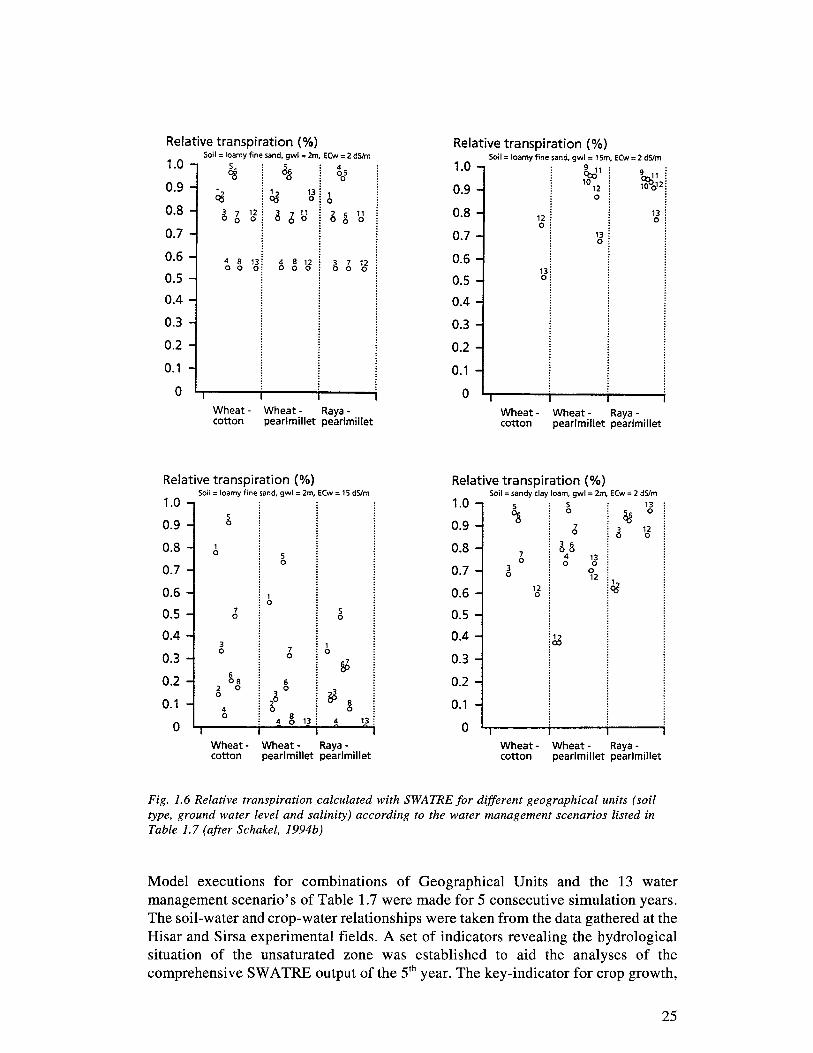
Fig. 1.6 Relative transpiration calculated with SWATREfor different geographical units (soil type, ground water level and salinity) according to the water management scenarios listed in Table 1.7 (after Schakel, 1994b)

Model executions for combinations of Geographical Units and the 13 water management scenario's of Table 1.7 were made for 5 consecutive simulation years. The soil-water and crop-water relationships were taken from the data gathered at the Hisar and Sirsa experimental fields. A set of indicators revealing the hydrological situation of the unsaturated zone was established to aid the analyses of the comprehensive SW ATRE output of the 5th year. The key-indicator for crop growth,

25

relative transpiration (Taclfpot)' is shown in Figure 1.6 for wheat-cotton, mustard-pearl millet and wheat-pearl millet crop rotations. The relative transpiration was calculated for different initial water table depths (2 m and 15 m), different salinity levels (2 and 15 dS/m) and different soil types (loamy fine sand and sandy clay loam).

Not all combinations of Geographical Units and water management scenario's were considered as drainage is a less usefull solution for deep water table conditions. Figure 1.6 exhibits that scenario 5 is rather favourable, which is not surprising considering its full canal water supply and the unlimited options to discharge the drainage effluent. Furthermore, the deep drainage at 2.5 m (scenario 5) seems to create systematically more favourable crop growth conditions than the 1.5 m (scenario 1) while scenario 6 with A W has potential when the groundwater quality is still reasonable (2 dS/m). For salinized conditions, only scenario's with drainage are recommended. Because wheat-cotton performs better than the other rotation schemes on saline soil, the cultivation of cotton on saline prone areas of Haryana should be stimulated. The Mustard-pearl-millet rotation in Figure 1.6B reflect proper yields even with reduced canal water applications (scenario 12) which saves a tremendous amount of water. Hence, the natural variation of physical factors demand for a variable agricultural water management.

Other indicators such as the stability in water and salt storage, the required annual amount of canal water and the cumulative drainage effluent are equally important. The superior scenario for each Geographical Unit should therefore be determined on the basis of multi-objective decision techniques (Schakel, 1995). With these mathematical techniques, the contrasting objectives of maximum crop yield, a neutral moisture change and salt change, a minimum of canal water and a minimum of drainage water effluent, can be obtained in an objective fashion for large datasets.

Conclusions

The model SW A TRE has again proven to be a very versatile and powerful package which can be applied under numerous circumstances. Testing was done under conditions of limited data avaialability to stress that calibration and validation will always remain a very vital part of simulation modelling. The local calibrations as shown in the examples are required for precisely diagnosing the water and solute dynamics in the unsaturated zone. The accuracy of the model was clearly shown in calculations of annual water and salt balances.

Combinations of Geographical Units, dependent on practical guidelines, with regional GIS provides a sound basis to improve regional water management.

26

References

Agarwal, M.C. and S.S. Khanna, 1983. Efficient soil and water management in Haryana. Haryana Agricultural University, Hisar, India, 105 pp.

Bastiaanssen, W.G.M., 1992. Delimitation of a numerical simulation experiment with the SW ASAL T model for irrigated crops on the Hisar farm, India. Mission Report of the Indo-Dutch Operational Research Project, Haryana Agricultural University, DLO-Winand Staring Centre, International Activities Report 22, Wageningen, the Netherlands, 64 pp.

Bastiaanssen, W.G.M., R Singh, S. Kumar and M.C. Agarwal, 1994. Control of soil degradation by modified irrigation and drainage techniques. In: Behl et al. (Eds), Impact of modem agriculture on environment, Proceedings of Indo-German Conference, Dec. 1-3, 1993, CCSHAU, Hisar, India, 83-93.

Bastiaanssen, W.G.M., 1995. Modelling on-farm soil water and salt balances of irrigated vineyards, Mendoza, Argentina. International Activities Report 42, DLO­Winand Staring Centre, Wageningen, the Netherlands, 80 pp.

Beekma, J., Th.J. Kelleners, Th.M. Boers and Z.I. Raza, 1995. Application of SW ATRE to evaluate drainage of an irrigated field in the Indus Plain, Pakistan. In: L.S. Pereira et al. (Eds.), Crop-Water-Simulation Models in Practise, Wageningen Press, Wageningen, the Netherlands, pp. 141-160.

Belmans, c., J.G. Wesseling and R.A. Feddes, 1983. Simulation model of water balance of a cropped soil: SWATRE. Journal of Hydrology, 63(3/4): 271-286.

Boers, Th. M., M. de Graaf, R.A. Feddes and J. Ben-Asher, 1986. A linear regression model combined with a soil water balance model to design micro-catchments for water harvesting in arid zones. Agricultural Water Management, 11: 187-206.

Boesten, J.J.T.I. and L. Stroosnijder, 1986. Simple model for daily evaporation from fallow tilled soil under spring conditions in a temperate climate. Netherlands Journal of Agricultural Science, 34: 75-90.

Boesten, J.J.T.I. and A.M.A. van der Linden, 1991. Modelling the influence of sorption and transformation on pesticide leaching and persistence. Journal of Environmental Quality, 20: 425-435.

Clemente, RS., R de Jong, R.N. Hayhoe, W.D. Reynolds and M. Hares, 1994. Testing and comparison of three unsaturated soil water flow models. Agricultural Water Management, 25: 135-152.

De Jong, R. and P. Kabat, 1990. Modelling water balance and grass production. Soil Science Society of America Journal, 54(6): 1725-1732.

27

Faria, R.T. de, C.A. Madramootoo, J. Boisvert and S.O. Prasher, 1994. A comparison of the performance of SW ACROP and the versatile soil moisture budget models in Brazil. Canadian Journal of Agricultural Engineering, 36: 1-12.

Feddes, R.A., P.J. Kowalik and H. Zaradny, 1978. Simulation offield water use and crop yield. Simulation Monograph. PUDOC, Wageningen, the Netherlands. 189 pp.

Feddes, R.A., P. Kabat, P.J.T. van Bakel, J.J.B. Bronswijk and J. Halbertsma, 1988. Modelling soil water dynamics in the unsaturated zone - state of the art. Journal of Hydrology, 100: 69-111.

Feddes, R.A. and A.L.M. van Wijk, 1990. Dynamic land capability model: a case history. Philosophical Transactions of the Royal Society, London B., UK, 329: 411-419.

Feddes, R.A. and W.G.M. Bastiaanssen, 1992. Forecasting soil-water-plant­atmosphere interactions in arid regions. In: H.J.W. Verplancke et al. (Eds.). Water saving techniques for plant growth. NATO-series: 57-78.

Genuchten, M.Th. van, 1980. A closed form equation for predicting the hydraulic conductivity of unsaturated soil. Soil Science Society of America Journal, 44(5): 892-898.

Huygen, J., G. Jacucci, P. Kabat, L.S. Pereira, P.J. Verrier, P. Steduto, C. Uhrik, J.L. Teixeira and J. Vera Munoz, 1995. The HYDRA Crop Growth Simulation System. Proceedings of the International Conference on Land and Water Resources Management in the Mediterranean Region, September 4-8, 1994, Bari, Italy.

Kabat, P., B.J. van den Broek and R.A. Feddes, 1992. SWACROP: a water management and crop production simulation model. In: L.S. Pereira et al. (Eds), Special Issue on Crop-Water Models, ICID Bulletin, 41(2): 61-84.

Kumar, S. and W.G.M. Bastiaanssen, 1993. Simulation of the water balance in relation to crop water requirements in (semi)arid zones. Question 44, R 28, The Hague, the Netherlands, 349-363.

Kumar, S., 1995. Suitability of simulation techniques on reuse of drainage water. In: K.V.G.K. Rao et al. (Eds.), Reclamation and management of waterlogged saline soils, CSSRI and CCSHAU, Central Soil Salinity Research Institute, Kamal, India, 331-346.

Makkink, G.F., 1957. Testing the Penman formula by means oflysimeters. Journal of International Water Engineers, 11: 277-288.

Menenti, M. 1994. Do Irrigation agencies and farmers need computational decision support tools? Proceedings of the International Conference on Land and Water Resources Management in the Mediterranean Region, September 4-8, 1994, Bari, Italy, 1061-1081.

28

Menenti, M., 1995. Analysis of regional water resources and their management by means of numerical simulation models and satellites in Mendoza, Argentina. In: S.P. Simonovic et al. (Eds.), IAHS Publication 231: 49-59.

Mirabile, c., 1990. Evaluacion y ensayos de campo en el area piloto de recupracion de suelos degrados por drenaje y salinidad en el departamento de Lavalle Mendoza. Proyecto FAO-Instituto Nacional de Ciencia y Technica Hidricas, Centro Regional Andino (INCYTH-CRA), Mendoza, Argentina, (in Spanish).

Monteith, J.L., 1965. Evaporation and the environment. In: The state and movement of water in living organisms, Proceedings XIXth Symposium Society of Experimental Biology, Swansea, Cambridge University Press 19: 205-234.

Penman, H.L., 1948. Natural evaporation from open water, bare soil and grass. Proceedings of the Royal Society, Land Ser. A, 193: 120-145.

Prasad, R., 1988. A linear root water uptake model. Journal of Hydrology, 99: 297-306.

Priestley, C.H.B. and R.J. Taylor, 1972. On the assessment of the surface heat flux and evaporation using large scale parameters. Monthly Weather Review, 100: 81-92.

Ragab, R., F. Beese and W. Ehlers, 1990a. A soil water balance and dry matter production model: I. Soil water balance of oat. Agronomy Journal, 82: 152-156.

Ragab, R., F. Beese and W. Ehlers, 1990b. A soil water balance and dry matter production model: II. Dry matter production of oat. Agronomy Journal, 82: 157-161.

Richards, L.A., 1931. Capillary conduction of liquids through porous mediums. Physics, 1: 318-333.

Ritsema, H.P. (Ed.), 1994. Drainage Principles and Applications. ILRI Publication 16, second edition (completely revised), International Institute for Land Reclamation and Improvement, Wageningen, the Netherlands, 1125 pp.

Schakel, J.K., 1994a. A distributed approach to control waterlogging and salinization, an application study with the SWASALT model. Internal Note 307, DLO-Winand Staring Centre, Wageningen, the Netherlands, 80 pp.

Schakel, J.K., 1994b. Effect of different water management scenario's on waterlogging and salinization, irrigation and drainage compendium, Version 1.0. DLO-Winand Staring Centre, Wageningen, the Netherlands, 75 pp.

Schakel, J.K., 1995. FIRM, manual of an on-farm decision support system. Technical Document 38, DLO-Winand Staring Centre, Wageningen, the Netherlands, 143 pp.

29

Singh, R., 1995. On-farm irrigation planning through simulation models in semi -arid regions. In: K.V.G.K. Rao et al. (Eds.), Proceedings national seminar on reclamation and management of waterlogged and saline soils, CSSRI and CCSHAU, Central Soil Salinity Research Institute, Kamal, India, pp. 347-358.

Van den Broek, B.I. and P. Kabat, 1995. SWACROP: dynamic simulation model of soil water and crop yield applied to potatoes. In: P. Kabat et al. (Eds), Modelling and Parameterization of the Soil-Plant-Atmosphere System. A comparison of potato growth models. Wageningen Press, Wageningen, the Netherlands, pp. 299-333.

Van Dam, J.e., I.M.H. Hendrickx, H.C. van Ommen, M.H. Bannink, M.Th. van Genuchten and L.W. Dekker, 1990. Water and solute movement in a coarse-textured water-repellent field soil. Journal of Hydrology, 120: 359-379.

Van Dam, J .C. and R.A. Feddes, 1996. Modeling of water flow and solute transport for irrigation and drainage. In: L.S. Pereira et al. (Eds), Sustainability of Irrigated Agriculture, Kluwer Academic Publishers, the Netherlands: 211-231.

Wolters, 1992. Influences on the efficiency of irrigation water use. Ph.D. thesis, Technical University Delft, Delft, the Netherlands, 150 pp.

Work Group SWAP, 1994. SWAP 1993 Input instructions manual. DLO-Winand Staring Centre and Wageningen Agricultural University, Internal Note 291, DLO­Win and Staring Centre, Wageningen, the Netherlands, 66 pp.

Zepp, H. and A. Belz, 1992. Sensitivity and problems in modelling soil moisture conditions. Journal of Hydrology, 131: 227-238.

30

2 Groundwater approach to drainage design in irrigated agriculture (SGMP)

J. Boonstra!, Sultan A. Rizve and M.N. Bhutta3

1 International Institute for Land Reclamation and ImprovementlILRI, P.O. Box 45, 6700 AA Wageningen, the Netherlands

2 Netherlands Research Assistance ProjectlNRAP, 13 West Wood Colony, Thokar Niaz Baig, Lahore, Pakistan

3 International Waterlogging and Salinity Research InstitutelIWASRI, 13 West Wood Colony, Thokar Niaz Baig, Lahore, Pakistan

Introduction

To improve drainage design criteria, the Netherlands Research Assistance Project/NRAP, in collaboration with the International Waterlogging and Salinity Research InstitutelI­W ASRI in Lahore, Pakistan, executes field research at the Fourth Drainage Project near Faisalabad in Pakistan. The Fourth Drainage Project is located in the south-western part of the Rechna Doab. The Rechna Doab consists of the area between the Rivers Ravi and Chenab and comprises about 28,000 km2

• The Fourth Drainage Project includes two separate areas, Schedule I and II, covering a total of 55,000 ha. In an area of 31 ,000 ha, horizontal subsurface drainage systems are under construction. Determining the drainable surplus and the drainage coefficient are two of the objectives of the on-going research in this Project.

Schedule I-B was selected to study the extent to which the assessment of the required drainable surplus could be refined. The area comprises some 90 km2 and is typified by its flatness. Schedule I-B belongs to the Samundri Unit II and is bordered in the north and south by two irrigation canals (i.e. the Lower Gugera Branch Canal and the Burala Branch Canal, respectively), by the Maduana Branch Drain in the west, and the city of Satiana in the east. In this area, eleven sump units with collectors and fields drains have been installed to alleviate waterlogging and salinity (Figure 2.1).

A methodology that uses a groundwater approach was developed to assess the drainable surplus for an irrigated agricultural area. Four components can be distinguished in that methodology: (i) Assessing historical net recharge to an underlying aquifer system based on a

groundwater-balance approach (ii) Decomposing this net recharge into its contributing components of recharge and

discharge, and assessing their order of magnitude (iii) Assessing the design net recharge by adopting a rainfall-recharge methodology (iv) Assessing areas in need of drainage and their drainable surplus based on design net

recharge.

The application of this overall methodology to Schedule 1-B of the Fourth Drainage Project is the subject of this paper.

31

to Dijkot o 2 3 4km I I I I

I I I , ,

I I

Talya'a disly / ~

surface d, ain

irrigation canal

road

.~/ ,. ______ K------ subsurface drains I i"'f·------- wilh sump unil no. ~~J

.. "'I ","'I -----~I

?' sadduwaladr~C~JU-. i

.' ' " ' I \ \ Ahmadabad Try drain 6! \ i \ ,----------

0---1 " , /Ei: L~ I

-------1 ~I \ \ \ \ \ \ d \ t ___ L.o-J \~I 10 \ ,-

/-----~:--"7 11 L _____ _ , , I

I , ' l~_T!.Y2~!!!1.. __ - l... __ _

\-'-\ I:: I \ I \:' i----_l._.§i~.!!<!'.I~~~C!!~!!!."---: ~ ______ L__: '\_ .!..3 ~ j------

,,:Jt--, I I ,I I r-------

,: : : I I I I ': ,----;." , , I' \F... :---

, , : ,'------- ' ~--~-.-.;,.' ~-----. , , ,y-------- , '

i , , ' , , I I I I , , ' 9------\ ___ L___ 9

17--=--....r .. ~,.'

-----..;;;.-!,1

I I

I r--_ I -----"'1----' -_............. \

" '6 _____ _ "', -----::9-:..::----~i .... ;_----.I I , ___ _ , .... , >', ~ I, I ~ _________ _

~ b I' \ ~jl=jr=_:::=:::=:c=====fi..=-=-=-=-=-=-=-=-=-=-·=='!.. I ~---,---- ~ '" \ I 51 :

1_---.

1(;----........ '''h; ......... rt/sly

\ I ....... Q---- f ____________ ~ : , _______ . '<' , ; I !

'"L___ ,--------------: : r-------" I '4 I

: : : ,11 : ,---- i-------: :: : 'I : . ,: ' I ' &" ' 1 __ ' 1 L "," : ,-----0-...' -----

0"4 ' : ' ' - --I I.,,~ \ ---1 r-----C);';'1- " _____ L ____ .... c::::::--" L----,ti'.t:.-Tiy-dra!:' J=.:::*'=-:.;-l--__ ----

~,," --------- I

------~-----. , I _____ L ______ .

Burala Branch canal

.... _--, ,

Balochwala minor

, ... , \ ,

\ , , --" ,', , to Tandlianwala to Tandlianwala

Fig. 2.1 Schedule 1-B area showing the location of the eleven sump units

~ I \ , ,

Nodal net recharge by inverse modelling

Moghal et al. (1992) reported on the development of a numerical groundwater model for Schedule I-B area. The relevant aspects of this report are summarized here. The groundwater model used is an updated version of the ~tandard Groundwater Model f.ackage, SGMP (Boonstra and De Ridder, 1990).

Numerical groundwater modelling requires a discretization in space. In SGMP, this is done using a nodal network. A distinction is made between internal and external nodes. The internal nodes are each representative for a nodal area, whereas the external nodes act as boundary conditions. The discretization in space resulted in a nodal network for Schedule I-B as depicted in Figure 2.2. This figure shows that the nodal network consisted of 56 nodes. Out of these 56 nodes, 24 external nodes acted as boundary conditions; these nodes are referred to as boundary nodes. The remaining 32 nodes represented the internal nodal areas; their size varied from 0.3 to 3.0 km2 with an average size of 1.6 km2

• These internal nodal areas represented the model area and comprised some 66 km2

• From here on, this area is referred to as S-I-B area (hatched area in Figure 2.2).

Based on geological reports, groundwater hydrographs and watertable contour maps, the aquifer system underlying Schedule I-B was treated as a homogeneous and isotropic unconfined aquifer. The aquifer thickness ranges from 180 m in the upstream part of Schedule I-B to some 210 m in the downstream part. In the model runs, different sets of aquifer-parameter values were adopted to allow for the ranges resulting from the various aquifer test analyses: the value of the horizontal hydraulic conductivity was taken as 20, 30, and 40 mid, while values of 5, 10, and 15% were used for the specific yield. The Basic Model Run constituted the mean values of the hydraulic conductivity and specific yield, being 30 mid and 10%, respectively.

As initial conditions the watertable elevations based on June 1985 readings were prescribed for all 56 nodes. The boundary conditions were the watertable elevations at the 24 boundary nodes at specified moments in time. The watertable elevation data observed bi-annually in June and October were regarded as being representative for the pre-monsoon and post-monsoon conditions. The model was run for the period June 1985 to June 1990 with a variable time step of 4 and 8 months, alternately.

Usually, watertable elevations at the internal nodes are calculated as a function of prescribed net recharge values which may vary in space and time. Based on these calculated watertable elevations, the various relevant water-balance components -horizontal subsurface incoming and outgoing groundwater flow, change in groundwater storage - are calculated for each internal nodal area. When SGMP is run in this manner, it is referred to as running in normal mode.

33

to Tandlianwnla to Tandlianwala

Fig. 2.2 Nodal network map for Schedule /-B area

o 2 3 4 km I I I I

I LEGEND:

----------- surface drain

Irrigation canal

road

roodel area with nodel number

In the so-called inverse mode, net recharge values in the internal nodal areas are calculated as a function of prescribed, historical watertable elevations at these nodes. All the simulation runs with SGMP in Moghal et al. (1992) were made in inverse mode. This resulted in ten sets of seasonal nodal net recharge values, five sets for monsoon and five sets for non-monsoon periods, in total 320 nodal net recharge values per run. Due to the range in hydraulic conductivity and specific yield values, sensitivity runs were made in this respect, resulting in five sets of different hydraulic characteristic values. Because of discrepancies in reported NSL values from SMO and FDP, sensitivity runs were also made in that respect, resulting in two sets of different absolute watertable elevations. Based on sensitivity analyses, the highest average net recharge value for S-I-B area ranged from 0.2 to 0.9 mm1d with a most probable value of 0.6 mmld for the monsoon of 1986; the return period for this monsoon was calculated as 2.8 years. The reported range in net recharge values could have been considerably smaller had the historical watertable elevations been known with an accuracy of a few centimetres.

Decomposition approach

With inverse modelling, the net recharge towards an underlying aquifer can only be assessed as a lumped value; this overall net recharge is actually composed of various contributing recharge and discharge components. The following recharge and discharge components with respect to the groundwater system were distinguished:

with Qne! = net recharge rate to aquifer Qrr = recharge from rainfall Qdr = recharge from distributaries Qir = recharge from water courses and irrigated fields Qcr = discharge by capillary rise Qpr = discharge by private tubewells QPll = discharge by public tubewells QSll = discharge by sump units of sub-surface drainage systems

(2.1)

The recharge by branch canals was not explicitly one of the components contributing to the net recharge of S-I-B area, because the nodal network was confined to an area in between the Lower Gugera and Burala Branch Canals. The losses of these two branch canals were, however, implicitly accounted for in the historical, observed watertable elevations at the external nodes which acted as head-controlled boundaries to the groundwater model.

The various components contributing to the overall net recharge, i.e. the terms on the right-hand side of the equals sign in Equation 2.1, were obtained in a tuning procedure.

35

Tuning procedure In the tuning procedure, the unsaturated zone was treated as a black box. A distinction was made between readily available data and so-called transform functions. The first are referred to as basic data.

The basic data consisted of daily rainfall data, daily head delivery discharges of the various distributaries and minors, land use data, depth to watertable data, Class A Pan data, and monthly drafts of private, public and sump unit tubewells. It was decided not to change any of these data in the tuning procedure.

The transform functions were as follows. Recharge by rainfall was estimated according to the Maasland procedure (Maasland et aI., 1963); in this procedure rainfall recharge is related to areal rainfall, land use, and cropping pattern. Recharge by irrigation was done on a water-balance basis: separate loss factors were introduced for distributaries, minors, water courses, and in the fields. Discharge by capillary rise and subsequent evapo(transpi)ration was related to watertable depth, soil type, pan evaporation, land use, and irrigation scheduling. Reduction in tubewell discharge was related to loss factors in water courses and in the fields. From a literature review, ranges for each of these transform functions were established prior to the tuning. It was decided not to exceed any of these ranges in the tuning procedure.

A series of interlinked spreadsheets was developed in which the basic data were fixed and the corresponding transfer functions were represented as parameters to be changed within certain limits.

Tuning criteria The tuning results were evaluated on the basis of the following criteria: (i) Minimum differences between seasonal nodal net recharge values resulting from

inverse modelling with SGMP and those calculated with the decomposition approach;

(ii) Minimum differences between watertable elevations as simulated by SGMP in normal mode using the nodal net recharge values from the decomposition approach and those observed in the field; and

(iii) Minimum differences between seasonal average net recharge values for S-I-B area as an entity resulting from inverse modelling with SGMP and those calculated with the decomposition approach.

The first criterion is the most strict one, because when the results satisfy the first criterion, they will automatically satisfy the third criterion. The opposite, however, is not true. Results may satisfy the third criterion, while not satisfying the first one. The second criterion is usually taken as the major criterion to calibrate numerical groundwater model applications. In this study, it was only taken as a relative criterion, because substantial differences in nodal net recharge values resulted in relatively small differences in simulated watertable elevations because of the large aquifer transmissivity values.

36

Tuning results Based on all three criteria, the parameter values in the transform functions were optimized. The final results can be summarized as follows; it should be noted that they are expressed as loss percentages contributing to groundwater recharge: monsoon rainfall: 20-30%; non-monsoon rainfall: 15-20%; distributaries: 6-8%; water courses: 10-15%; fields: 6-11 %.

In most water-balance studies, a differentiation is made between losses from the irrigation system on the one hand and irrigation losses recharging the groundwater on the other hand; in the tuning procedure only the latter could be evaluated. As an illustration of the results, Figure 2.3 shows the comparison between seasonal areal average net recharge values based on the above parameter values with those from the inverse modelling results (Basic Model Run).

Figure 2.3 shows that there is good agreement between the two sets of areal average net recharge values, except for Season 9 (monsoon 1989), where the net recharge is significantly higher than it is according to the Basic Model Run. There was no possibility to improve on the result of this season, unless the basic data are adjusted.

average areal net recharge in mm/d 1.0 ~------------------------------------------------~

0.8

0.6

0.4

0.2

o

-0.2

-0.4

~ decomposition

approach •

• •

•

-0.6~--~--~--~--~~--~--~--~--~8----9~--~1~0~

seasons

Fig. 2.3 Comparison of seasonal average areal net recharges based on the decomposition approach and on the inverse modelling result (Basic Model Run)

Design nodal net recharge

Usually, a historical study period will not comprise a monsoon season which is representative for a design monsoon. This implies that a set of synthetical nodal net

37

recharge values should be made. In this study, they were based on the values calculated for the wettest monsoon in the study period from inverse modelling and their rainfall recharge values were substituted by those of the design monsoon; in this substitution procedure the rainfall recharge methodology and parameters were adopted from the tuning procedure.

The wettest monsoon in the study period occurred in 1986 with 282 mm rainfall and a return period of 2.8 years (Boonstra et aI., 1991). For design purposes it is common in Pakistan to take a one-in-5-year wet monsoon. Based on the same frequency analysis, the total rainfall depth in such a design monsoon was calculated as 347 mm.

Table 2.1 presents design net recharge values for the various nodal areas separately as well as an average value for S-I-B area. The latter is according to Table 2.1 equal to 0.7 mm/d, which is only 0.1 mm/d more than the historical corresponding value for monsoon 1986 (Moghal et aI., 1992). A similar slight increase in this value between monsoon 1986 and the design monsoon was reported by Rizvi (1993).

The value of 0.7 mmld is based on the inverse modelling results from the Basic Model Run. In the tuning procedure, the results of this run gave the best comparison with the results from the decomposition approach. This implies that without the results from the tuning procedure, the average design net recharge for S-I-B area would have been presented as a range, from 0.3 to 1.0 mmld.

To check whether the groundwater condition during the monsoon 1986 was representative for design monsoon conditions, SGMP was run with the design net recharge values of Table 2.1 as substitute for the historical monsoon 1986 net recharge values. The calculated watertable elevations in this run were not more than 10 cm higher than those at the end of monsoon 1986. Because of this, we concluded that the calculated capillary rise rates for that monsoon were also representative for the synthetical design monsoon.

Table 2.1 Synthetical design monsoon nodal net recharge values.

nodal design qnet nodal design qnet nodal design qnet

area (mm/d) area (mm/d) area (mm/d)

3 2.1 24 1.3 37 1.0 4 0.8 25 0.8 40 2.3 7 1.8 26 0.0 41 0.9 8 0.8 27 0.1 42 0.3

11 1.6 28 0.3 43 0.7 13 0.2 29 0.4 46 0.8 14 1.3 30 0.4 47 0.7 17 0.4 33 0.7 49 -0.8 18 0.3 34 0.9 51 0.1 19 0.6 35 0.4 52 0.4 22 1.5 36 0.5

38

In addition, there is also no reason to assume that the irrigation deliveries during a design monsoon will be different from the monsoon 1986 deliveries. In other words, apart from a different rainfall recharge, all the other calculated recharge and discharge components contributing to the net recharge can thus be taken to be representative for a design monsoon.

Considerations on drainable surplus

Drainable surplus is here defined as the quantity of water that must be removed from an area within a certain period so as to avoid an unacceptable rise in the groundwater level. Drainage coefficient is sometimes used as a synonym for drainable surplus although it is usually limited to a short period, in the order of days. This study can only present an assessment for the drainable surplus, because of the seasonal time step of 4 and 8 months.

The question to be addressed here is to what extent the net recharge can be regarded as a measure for the drainable surplus, i.e. which of the components contributing to the net recharge should be considered for assessing the drainable surplus. To this end, we present the following considerations: - Recharge components from rainfall and irrigation: there is no discussion, as they are

also part of the drainable surplus in the traditional drainage design. - Discharge by capillary rise: this will also occur during a design monsoon. It should

be a discharge component contributing to the drainable surplus, although it is not a part of it in the traditional drainage design.

- Discharge by private tubewells: it depends whether farmers will pump less groundwater or no groundwater at all during a design monsoon. Most probably farmers will gradually realize that a particular monsoon is extremely wet, i.e. they will reduce their pumping sometime during such a monsoon period. It is often assumed, however, that private tubewell pumping should not be part of the drainable surplus.

- Discharge by public tubewells: it depends whether the new drainage system under consideration should replace all the existing drainage systems or whether it should be regarded as an additional system. In the first case, it is obvious that it should not be a discharge component contributing to the drainable surplus and in the second situation, it is equally obvious that it should.

For this study, the conservative approach was followed: both private and public tubewell pumping should not be a discharge component contributing to the drainable surplus. The drainable surplus can thus be described by:

(2.2)

Different assessments for the drainable surplus will be presented based on the groundwater approach, which is actually a combination of the bottom-up and top-down approach. It integrates the groundwater recharge resulting from the various water balance components at the land surface with the contribution from the aquifer itself, i.e. lateral groundwater in- and outflow, capillary rise and change in groundwater storage.

39

Drainable surplus without induced groundwater flow For the assessment of the drainable surplus as described by Equation 2.2, two different approaches were followed. The first approach to assess the drainable surplus is based on the bottom-up approach. The net recharge is based on the lateral groundwater in- and outflow and change in groundwater storage, and its lumped value is assessed using the inverse modelling results. This value implicitly represents all the contributions of relevant recharge and discharge components as summarized in Equation 2.1. So, the contributions of the various tubewell pumping should be eliminated from its value in order to assess the drainable surplus according to Equation 2.2. The value of the average drain able surplus can thus be described by:

(2.3)

It should be noted that Qne! in Equation 2.3 represents the design net recharge; the historical net recharge based on the inverse modelling results thus needs to be adjusted for increased rainfall recharge during a design monsoon. During the monsoon of 1986 no sump units were operational, so Qsu was equal to zero.

A second approach to assess the drainable surplus is based on the top-down approach, i.e. directly on Equation 2.2. The values of its recharge and discharge components were assessed from the tuning procedure, except rainfall recharge; for its value, the design rainfall recharge was substituted. The average drainable surplus according to the second approach then yields:

(2.4)

Both approaches would result in identical estimates for the drainable surplus when the tuning procedure yields a perfect match between the two sets of net recharge values.

Drainable surplus with induced groundwater flow The assessment of the drainable surplus is usually made without considering the relationship between drainable surplus, minimum permissible depth-to-watertable, and areas in need of drainage. This relationship was found by running SGMP in normal mode.

In SGMP, there is a provision to prescribe upper levels of the water table, which may not be exceeded in a simulation run. If during a particular period the calculated watertable elevations would exceed such an upper level, SGMP introduces an artificial drainage component to keep the calculated watertable elevation just below that level. These upper levels can be regarded to represent the minimum permissible depth-to­watertable, to be controlled by a subsurface drainage system and the artificial drainage rate to represent its required drainable surplus. In reality, the watertable depth between two drains will be smaller than the actual drain depth. This can be accounted for by taking the average of minimum permissible watertable depth midway between the drains and actual drain depth.

40

To determine the relationship between drainable surplus, minimum permissible depth­to-watertable, and areas in need of drainage, the drain able surplus values were calculated according to Equation 2.3, thus eliminating the tubewell component from the design net recharge. Next, a particular drainage strategy was required. The areas which were originally designed to have subsurface drainage, i.e. the eleven sump units in S-I-B area (Figure 2.1), were selected as potential areas in need of drainage. In other words, the drainage strategy of USBR was adopted. Since the area drained by a particular sump unit does not fully coincide with one or more of the nodal areas of SGMP's nodal network, the following rule has been used: if more than 50% of a nodal area is drained by a sump unit, this nodal area was selected as a potential area in need of drainage (hatched areas in Figure 2.4).

To these nodal areas certain upper levels of the water table were recognised; these levels represented the average natural surface elevations in the nodal areas minus average permissible depth-to-watertable. For various permissible depths-to-watertable simulation runs were made with SGMP. Figure 2.5 shows the results of these runs simulating a subsurface drainage system with a permissible depth-to-watertable of 1.5 m below land surface.

The results of this run can be summarized as follows: (1) out of the 21 nodal areas which were in need of drainage according to the original USBR design, only 11 nodal areas need artificial drainage according to the present study and (2) an average value of 1.3 mmfd for the required drainable surplus is found in this study, whereas in the original design the drainage coefficient was taken as 2.4 mmfd.

All simulation runs with SGMP were done on a seasonal basis, because data on watertable depth were only available on a bi-annual basis during the study period 1985-1990. This implies that the drainable surplus of 1.3 mmfd is an average value over the four months of a monsoon period. In reality, higher values will occur during shorter periods. So, the drain able surplus may not be considered to be a measure for the drainage coefficient. This aspect needs further study.

Discussion of results

A groundwater-balance approach was used to assess the regional and nodal net recharge for Schedule I-B of the Fourth Drainage Project. To this end, a groundwater model was used in inverse mode. For this approach, data on the geometry of the aquifer system, its hydraulic parameters, and historical watertable elevations were collected from the field. The resulting net recharge is a lumped parameter: all the relevant contributing recharge and discharge components are integrated in its value. This net recharge can be regarded to be representative for a historical period, provided that the watertable elevations are determined with sufficient accuracy.

41

10 Dijkol

......

BUr ala Branch canal

to Tandlianwala 10 Tandlianwa!a ~

o 2 3 4km

\ ,

I I I I

I

... , , ... -, .......

~

----------- surface drain

-------- irrigation canal

======= road

~area in need of drainage ~according to original design

", \ I ,

... ,

Fig. 2.4 Representation in SGMP of the areas in need of drainage in S-/-B area according to original USBR design

(0 Tandlianwala to T:::mrlli:lnw::l;1:r.

o 2 3 4km I I I I

I

-~

LEGEND:

----------- surfacedrain

-irriga1ion canal

load

area in need of drainage according 10 SGMP

'" , I

" ,

Fig. 2.5 Areas in need of drainage in S-I-B area according to SGMP with an average permissible depth-to-watertable of 1.5 m

The advantage of assessing the net recharge with the groundwater-balance approach is that far fewer data are required. For instance, to assess the same net recharge by integrating the water balance for the unsaturated zone with the water balance at the land surface would require considerably more data: e.g. data on rainfall, irrigation, seepage from open water bodies, crops, soils, and tubewells. Collecting and processing these data, many of which vary in space and time, is time-consuming, and their reliability is sometimes questionable. Hence, using a groundwater-balance approach with inverse modelling to assess the net recharge to an aquifer system deserves more attention than it has been given. Moreover, if simulation models based on the integrated water-balance approach will be used, the groundwater-balance approach can then serve as a check on the results of these models.

A rather simplified and rigid procedure was applied to assess the contribution of relevant recharge and discharge components to the overall net recharge value for the aquifer. The methodology described had as a major objective the development of a calculation algorithm where all the contributions were linked to each other. This implies that all the existing opinions on the order of magnitude of various contributions could be systematically evaluated using the inverse modelling results from SGMP as a benchmark.

An integrated approach was followed taking into account all the relevant recharge and discharge components contributing to the drainable surplus. In the assessment of the drain able surplus two different approaches were used. The first approach did not include the change in lateral groundwater flow induced by lowering the watertable as a result of the various sump units. The drainable surplus can then be represented as the design net recharge corrected for tubewell pumping. Within this approach two assessments of the drainable surplus were presented: one based on the inverse modelling results and the other based on the decomposition results. The second approach did not only include the change in lateral groundwater flow, but also introduced the relationship between drainable surplus and minimum permissible depth to watertable. This could only be simulated with groundwater models. This approach yielded a re-assessment of the areas in need of drainage.

Finally it should be noted that no values for the drainage coefficient could be presented, because data on watertable depth were only available on a bi-annual basis during the study period 1985-1990. This is not a limitation of the methodology presented; the same methodology could have resulted in an assessment of the drainage coefficient if the depth-to-watertable data would have been observed at shorter intervals than at the present seasonal interval. The difference between drainage coefficient and drainable surplus is actually only due to the difference in rainfall recharge; the other components of drainable surplus are also representative for the drainage coefficient.

Acknowledgements

The research for this paper was conducted in the framework of the Netherlands Research Assistance Project (NRAP), Lahore, Pakistan, a joint project of IW ASRI

44

and ILRI sponsored by the Governments of Pakistan and The Netherlands. The authors appreciate the financial support received for this study.

References

Boonstra, J. and N .A. de Ridder, 1990. Numerical modelling of groundwater basins (2nd. ed.). ILRI Publication 29, Wageningen, the Netherlands.

Boonstra, J., Ashraf M. Moghal, Syed Hamid Ali and W.F. Vlotman, 1991. Collection, processing and screening of data for the S-I-B Area of the Fourth Drainage Project. NRAP Report 30, Lahore, Pakistan.

Maasland, M., J.E. Priest and M.S. Malik, 1963. Development of groundwater in the Indus Plains. Pakistan Engineering Congress, Lahore. Symposium on Waterlogging and Salinity, Proceedings, Vol. 7, Paper No. 56, 123-161.

Moghal, Ashraf M., Syed Hamid Ali and J. Boonstra, 1992. Seasonal net recharge to aquifer underlying the schedule I-B Area, June 85 - June 90, Fourth Drainage Project. NRAP Report 33, Lahore, Pakistan, 127 pp.

Rizvi, Sultan A., 1993. Prediction of drainable surplus for Fourth Drainage Project Faisalabad. A thesis for the degree of Master of Philosophy in Water Resources Management. CEWRE, University of Engineering & Technology, Lahore, Pakistan.

45

3 Computer program for flume and weir design* (FLUME 3.0)

A.J. Clemmensl, M.G. BOS2, J.M. Groenestein3 and J.A. Reploglel

2

3

u.s. Water Conservation Laboratory, 4331 E. Broadway Road, Phoenix, AZ 85040, U.S.A. International Institute for Land Reclamation and ImprovementlILRI, P.o. Box 45, 6700 AA Wageningen, the Netherlands Groenestein en Borst vof, Costerweg 5, 6702 AA Wageningen, the Netherlands

Introduction

FLUME 3.0 is a useful computer program for the design and calibration of critical­depth, open-channel, long-throated, flow-measuring structures, e.g. the long-throated flume and the broad-crested weir. It matches the user's requirements for flow measurement with the hydraulic conditions of the channel in which the measuring structure is to be placed. It allows the user to enter data conveniently with pull-down menus and graphical data entry screens.

For existing structures, the graphical data entry screen can be used to enter data on the channel, the flume profile, and the cross section. The user can select from among a variety of cross-section shapes. These cross sections are drawn to scale and can be superimposed upon one another to assure that the correct dimensions have been entered.

FLUME 3.0 provides a variety of reports, including flume input data, flume design results, rating tables, equations, and field data comparisons. Many of the reports are also available as graphs. The FLUME 3.0 database keeps track of all flume designs, as-built dimensions, rating tables, and field data. A variety of units can be chosen for depth, discharge and flow velocity.

Theory

Critical depth theory has been known for more than a century. Although this theory assumes an ideal (frictionless) fluid and ideal hydrostatic pressure distributions (no streamline curvature), water flow is influenced by friction, and real flumes and weirs cause some streamline curvature. Long-throated flumes and broad-crested weirs minimize streamline curvature and its effects.

* Presented at the ASCE (Irrigation and Drainage Division) conference: Management of Irrigation and Drainage Systems, 21-23 July 1993, Park City, Utah, U.S.A.

Preceding page blank 47

Replogle (1975) devised a computational scheme to account for the influences of friction. His scheme calculated the discharge for known values of the upstream water depth. These computations have proved accurate enough for long-throated flumes to be used in the field without laboratory calibrations.

One of the major problems for the designer of critical-depth flumes and weirs in practice is to install the devices without allowing downstream submergence to influence the discharge reading. Bos and Reinink (1981) developed a method to determine the amount of head loss required between upstream and downstream levels to assure that critical flow continues to exist. The critical-depth theory of Replogle (1975) and the head-loss calculation of Bos and Reinink (1981) were combined in FLUME to aid in the calibration and design of critical-depth flumes and weirs (Clemmens et aI., 1987).

The main dimensional requirements of these flumes and weirs are given in the FLUME 3.0 user's manual (Clemmens et aI., 1993). Guidelines on recommended channel conditions are provided in FLUME 3.0 and in the user's manual.

Some of the advantages of critical-depth flumes and weirs are: - Provided that the critical flow occurs in the throat, a rating table can be calculated

with an error of less than 2% in the computed discharge. Rating tables can be calculated for any combination of a prismatic throat and an arbitrarily shaped approach channel; The throat, transverse to the direction of flow, can be shaped so that a range of discharges can be measured accurately, and no excessive backwater effect is created; The head-loss requirement over the weir or flume to obtain modular flow, i.e. the unique relationship between the upstream sill referenced head, hI' and the discharge, Q, is minimal; The head-loss requirement can be estimated with sufficient accuracy for any critical-depth weir or flume in any arbitrary channel; The gradually converging transitions prevent most problems with floating debris; Field and laboratory observations have shown that the structures can be designed to pass sediment transported by channels with subcritical flow; Provided that the throat is horizontal in the direction of flow, a rating table based upon as-built dimensions can be calculated, even if errors were made in construction to the designed dimensions. This as-built rating also allows the throat to be reshaped after initial construction, if required (Photograph 3.1); Under similar hydraulic and other boundary conditions, critical-depth weirs and flumes are usually the most economical of all structures for the accurate measurement of flow.

Design requirements

The design procedure for flumes and weirs is straightforward in some cases; in other cases, it can be quite complicated. Manual design procedures and rating tables for some standard types and sizes of flumes and weirs were presented in Bos et aI.

48

(1984). These procedures had the designer try different standard flumes and then evaluate whether or not they met the criteria on submergence and freeboard at maximum flow. More detailed manual design procedures, including consideration of accuracy and conditions at both minimum and maximum flows, are provided by Bos et al. (1986).

These manual design procedures are based on sufficient contraction in flow area for a given, desired, upstream water level and flow rate. The Froude number of flow in the approach channel can be related to the area of the control and approach sections, to their top-width ratios, and to the exponent of the head-discharge relation, u. The procedure is still iterative in that it is difficult to determine directly a shape with the correct values for these three variables.

Photo 3.1 FLUME 3.0 calculates a rating table based upon as-built dimensions

49

But even so, it is much quicker than trial and error for designers who are trying to determine head-discharge relations for the almost infinite number of possible structure shapes. These relations were expanded upon by Clemmens and Bos (1992) for FLUME 3.0 so that designers could conveniently calculate the mathematical values.

Design inputs The user provides the following basic design inputs: - Minimum and maximum flow rates;

Desired accuracy at minimum and maximum flow rates; Method of head detection (or accuracy of head detection); Existing discharge relationship in the channel stage (without flume); Shape and dimensions of the channel's cross section upstream and downstream from the measurement site (including canal depth); An initial shape, with dimensions, for the flume throat's cross section.

Design options The user can choose to define the maximum allowable upstream water level in one of two ways: - As channel freeboard as a percentage of upstream sill-referenced head; - As a fixed freeboard height.

If there is more head available at the site than necessary, the user can specify that a structure be chosen: - To minimize head loss; - To maximize head loss; - To be halfway between minimum and maximum head loss; - To make the head loss match the drop in channel bottom.

Structures can be designed with a fixed crest (the usual case) or with a vertically movable crest.

The program allows the user to choose a variety of cross-section shapes for flumes, and it does not require that all cross sections have the same shape. For example, the flume crest can be circular and the approach channel can be a trapezoid. The different shapes are shown in Figure 3.1. To design a structure automatically, the user must enter a reference shape for the throat. This is essentially a starting point for the design.

Next, the user must specify how the shape should be altered to arrive at a design. This input is necessary as there may be an infinite number of structures that will satisfy the design criteria. The options for shape modification are: - Contract the bottom (raise the bottom or add a bottom sill to the shape)

(Photograph 3.2); - Contract the sides (move the sidewalls in at the same side slope or reduce the

radius of the circle or the focus of the parabola); - Raise or lower the entire throat section relative to the approach section; - Raise or lower the inner section of a complex shape (move, for example, a

trapezoid up or down inside the circle).

50

Zc

~ ~, , bx '

v

simple trapezoid

rectangle

V-shaped

circle

U-shaped

parabola

~Zmid~ complex

D~et:apeZOid , ,( b' ),' : In 1 :C ): . bout .

~~in l()l--- -bc

Dc

J b===,{:

~I'--P' f1 ,---/::-------- In

._----------- +

trapezoid in circle

trapezoid in U-shape

trapezoid in parabola

sill in circle

sill in U-shape

sill in parabola

Fig. 3.1 The user can choose from seven shapes for the approach and tailwater channels. For the control section, fourteen shapes are available

51

Photo 3.2 The addition of a sill to the bottom of the canal creates a low-cost and accurate flow­measuring device

Design evaluation

From the above information, the program attempts to find a flume shape that will satisfy the user's design criteria. Sometimes, a variety of shapes will be acceptable. In these cases, the program checks the remaining dimensions (e.g. the lengths) to make sure they satisfy the requirements for long-throated flumes. If they do not, the user can modify them by rounding them to whole numbers where appropriate. The user can then check to see if this flume shape still meets the design criteria. The dimensions are stored in the FLUME 3.0 database. The user can also check the acceptability of any flume without going through the program's design calculations.

Once the program has produced either an acceptable design or a reasonable starting point for a design (if no acceptable design is found), it will provide a design report. An example is given in Figure 3.2. Design acceptability is decided by the following boundary conditions: - Allowable error in flow rate at minimum flow C.± two standard deviations); - Allowable error in flow rate at maximum flow; - Head loss at minimum flow; - Head loss at maximum flow; - Freeboard at maximum flow; - Froude number at maximum flow.

52

If all the design criteria specified in these conditions are met, a design will be found. If only some criteria are met, the program will suggest various ways to modify the shape of the flume, gradually guiding the user towards a feasible design according to which criteria are met and which are not. If the user follows the suggestions, the program will either find a feasible design or it will show that a feasible design with these design criteria is not possible.

User: Dr.Ir.M.G.(Rien) BOS Report made on: June 23, 1993 Flume: Phoenix, Phoenix, example structure used in manual Version 3

Report on all flume data.

GENERAL DATA ON FLUME Type of structure: Stationary crest. Type of lining: Concrete smooth Roughness height of flume: 0.00100000 m

BOTTOM PROFILE DATA

Length per section: Approach section = 2.000 m Converging ramp length = 1.200 m Control length = 1 .000 m Expansion length = 2.550 m

Vertical dimensions: Upstream channel depth = 1.250 m Height of sill = 0.425 m Bedlevel drop = 0.000 m Expansion ramp slope = 6.000:1

APPROACH SECTION DATA Section shape = SIMPLE TRAPEZOID Bedwidth = 1.000 m Channel side slope = 1.00:1

CONTROL SECTION DATA Section shape = SIMPLE TRAPEZOID Bedwidth = 1.800 m Channel side slope = 1.00:1

TAILWATER SECTION DATA Section shape = SIMPLE TRAPEZOID Bedwidth = 1.000 m Channel side slope = 1.00:1

Fig. 3.2 Example of a design report given by FLUME 3.0

In some cases, it may be that the basic flume shape should be modified. For example, if both a side contraction and a bottom contraction are required for a satisfactory design, the design calculations will not find that shape, as only one dimension is allowed to change at a time. The user can keep repeating the design calculations with new starting shapes until the program eventually arrives at a feasible shape (if a

53

shape is possible with the given design criteria). If the program indicates that a design is not possible, the user can relax the design criteria and try again. It may be that with less stringent specifications for accuracy or for freeboard limits, or with a different head-detection method, the program will find a reasonable design.

Databases, data entry and output

FLUME 3.0 maintains a database for flume dimensions and site conditions and a database for rating tables. When defining a new structure, the user can either copy an existing structure from the flume database or create a new flume with default data. The user can then alter the data to fit new site conditions, new flume dimensions, and new design requirements. If the physical dimensions of a flume are altered, the rating tables are not saved and will have to be recalculated. The program maintains a version number for each flume so that the user can check whether or not the flume dimensions and design reports match the rating tables, equations, and field-data reports.

A number of standard flumes are available in the initial database. The user can copy some of them to a new site to test their suitability there or to begin the design process. Together, the databases are an extremely useful feature of the program, helping engineers who design and construct flumes only infrequently, and providing a permanent record of as-built information on flow-measuring structures.

Graphical data entry FLUME 3.0 enables the user to enter flume dimensions in a graphics mode, where they are drawn to scale, so that the user can be sure the right shapes and dimensions are being chosen. The entry screen is illustrated in Figure 3.3. During the design process, the program uses several different data entry screens. They all display the same information, but data editing differs for each. For example, when defining channel conditions, the user can edit only the parameters which define the channel. When defining the initial control-section shape, the user can alter only those parameters which define the flume. When reviewing the design, the user can change the flume-crest width with the profile-sill height automatically, according to the design mode chosen.

An important feature of the program is data entry of cross-section dimensions on a scale drawing. With this, the control section, drawn to scale and with appropriate elevations, can be superimposed on the approach or on the tail water channel. The user can quickly see whether or not errors in data entry have been made and get a sense of how suitable the flume design is.

54

All dimensions are in m Channel depth 1.2513

BOTTOM PROFILE

S ill height 13.-+1313

Slope~ Slope 6.1313

.......... ....................................................................ir;;llililll:III.....llillllr .. rt. ~:::.:.:.o 0

2.131313 Approach

APPROACH SECTION

Slope 1.1313 ........ 1~··:·:···

-'::::::', ...... "::::~~~::::-. ,' ... '

'.::::::.:.:.;.:.:-:.:.:.:.:.::::,'

1.131313 Bedwidth

Section shape: SIMPLE TRAPEZOID

1.21313

Converge

1 . a a a Control

CONTROL SECTION

1 . a a a Bedwidth

Section shape: SIMPLE TRAPEZOID

Fig. 3.3 Graphical data entry screen

Reports and graphs

2.-+1313 Expand

Tailwater

TAILWATER SECTION

Slope 1.1313

1~:':':-:-' ........

.. ::::::.:.:-:.:.:.:.:.:.:.:.::::::{:/::"

1 . a a a Bedwidth

Section shape: SIMPLE TRAPEZOID

The program will generate rating tables for discharge at even intervals of depth and rating tables for depth at even intervals of discharge. The latter tables are useful in the manufacture of wall-mounted gauges marked with discharge units. Output from the program calculations is automatically saved in the database for future recall. The user specifies which data in addition to head and discharge are to be displayed in the output tables or graphs. The program generates reports that contain basic information so that the user can identify the flume for which data is displayed. These reports can be viewed on the screen, sent to a printer, and written to a disk file. The program can fit rating equations to the flume rating-table data, from which it can generate a report or a graph. Field data on depth and discharge can be entered for comparison with the rating table calculations. The program will compute a discharge for each measured value of head and generate a report or a graph for comparison of both values.

The program contains an OPTIONS menu that allows the user to manage the databases, set up the system (e.g. printer, display mode, and so on), and select units. FLUME 3.0 stores all data in SI units (e.g. m, m3/s, m/s) and displays all data in user-specified units. A variety of units are available for depth, discharge, and velocity.

55

References

Bos, M.G. and y. Reinink, 1981. Head loss over long-throated flumes. American Society of Civil Engineering Journal of the Irrigation and Drainage Division, 107(IR1): 87-102.

Bos, M.G., J.A. Replogle and A.J. Clemmens, 1984. Flow measuring flumes for open channel systems. John Wiley & Sons, New York, U.S.A.

Bos, M.G., A.J. Clemmens and J.A. Replogle, 1986. Design of long-throated structures for flow measurement. Irrigation and Drainage Systems, 1(1): 75-92.

Clemmens, A.J. and M.G. Bos, 1992. Critical depth relations for flow measurement design. Journal of Irrigation and Drainage Engineering, 118(4): 640-644.

Clemmens, A.J., M.G. Bos and J.A. Replogle, 1993. FLUME: Design and calibration of long-throated measuring flumes. Publication 54, ILRI, Wageningen, the Netherlands.

Clemmens, A.J., J.A. Replogle and M.G. Bos, 1987. FLUME: A computer model for estimating flow through Long-Throated measuring flumes. U.S. Department of Agriculture, Agricultural Research Service, ARS-57.

Replogle, J.A., 1975. Critical-flow flumes with complex cross-section. Irrigation and Drainage in an Age of Competition for Resources, 366-388. American Society of Civil Engineers, St. Joseph, Michigan, U.S.A.

56

4 A hydrodynamic model in the design of operational controllers for water systems (MODISIMA TLAB)

M.G.F. Wernert, J. Schuurmanst, H.J. Campfens2 and R. Brouwerl

1 Delft University of Technology, Faculty of Civil Engineering, Section of Land and Water Management, P.O. Box 5048, 2600 GA Delft, the Netherlands

2 HASKONING Royal Dutch Consulting Engineers and Architects, P.O. Box 151,6500 AD Nijmegen, the Netherlands

Introduction

In the operational design of water systems, hydrodynamic programs can be applied as a research tool. The designer of a water system can gain insight into the effect of proposed operational measures before they are actually implemented. Although the investment in the development of such a model is often substantial, the potential savings are much greater. In the past, although the water systems modelled were sometimes complex, the operational strategies applied and the controllers that generate instructions for the manipulation of adjustable structures was often kept elementary. The existing modelling packages, although often difficult to work with, are generally adequate in these cases. They are, however, in adequate for dealing with more complex problems that require more complex controllers.

Operational control systems are used to increase the effectiveness of the water system (Brouwer, 1993). The development of progressively more complicated operational control systems has led to the desire to have more freedom in the choice of algorithms that can be implemented in the model. At present, the user of a hydrodynamic modelling package is often required to perform a large amount of laborious low level programming. This is a very time consuming task, as this programming is usually done within the original source code, which is complicated and often not adequately documented (Burt, 1993).

A link between an existing hydrodynamic modelling program MODIS (MOdelling Drainage and Irrigation §ystems) and a flexible mathematical package MA TLAB may well be able to increase the flexibility of algorithm choice, as well as increasing user friendliness.

This paper investigates such a combination. The hydrodynamic program itself and the mathematical package, as well as the structure of the combination will first be discussed. The applicability will then be demonstrated through two case studies.

57

The hydrodynamic model: MODIS

The program MODIS was developed at the Delft University of Technology (Schuurmans, 1993). It was based on the hydrodynamic modelling package RUBICON, developed by HASKONING Royal Dutch Consulting Engineers and Architects (RUBICON, 1984).

The model uses the complete Saint Venant equations. These are solved using the implicit Preismann scheme (Schuurmans and Maherani, 1991). MODIS allows the user to model any open channel water system. The advantage of MODIS is that the user can change parameters of, for example, structures during simulation. The values of parameters can thus be made to depend on the simulated values of model variables. This makes it possible to model control systems in which, for example, the sill level of a weir is adjusted according to the water levels in the system. A number of operational control algorithms are pre-defined in MODIS and can easily be implemented in the model. The model also includes performance indicators, providing a useful tool for the evaluation of various operational control systems. However, if the control system to be investigated is not already available, then the user is required to program it as FORTRAN 77 code and link it with the model.

Through the experience of students using the MODIS package in the context of their graduation research it has become apparent that programming a user-defined algorithm to investigate operational strategies requires a sound knowledge of FORTRAN computer programming, as well as enormous patience, as the process is often frustrating and time consuming. It was found that even the use of pre-defined algorithms often required some reprogramming to suit the user's needs exactly. Through the combination of MODIS with a package which simplifies programming, a lot of time could be saved. The MATLAB package was found to be suitable.

The mathematical package: MATLAB

The MATLAB package has been under development for a number of decades. It was specifically developed to deal with numerical problems (MATLAB, 1993). The numerical computations in MATLAB are based on matrix calculations.

MA TLAB can also be seen as a programming language, as it is possible to write one's own routines. The advantage it has over FORTRAN and other low level languages is that it is a fourth generation, script based language. The programming syntax is simple and debugging is facilitated by the interactive nature of the program. A large number of mathematical functions have already been programmed. So-called toolboxes, containing more specialised procedures, are available.

Algorithms which are to be used, either user defined or part of the MATLAB package, are implemented via so-called M-files. These are ASCII files containing the source code of the routine. Once a number of operational algorithms have been developed, a library can be created, so that the user will in future be able to choose from a number of algorithms suited for use in water systems. These could

58

subsequently be customised as the M-files are easy to understand. A number of operational control algorithms as well as irrigation performance algorithms have already been developed as M-files. A simple example of an M-file is given below:

%PlotVectors: This M-file plots the vector y against the vector x plot(x,y);

where '%' indicates a comment line. If the M-file is saved under the name PlotVector.m then the plot will be drawn upon entering this name at the MATLAB command line, provided of course that x and y exist and have the same length.

Combination of MODIS and MA TLAB

The MA TLAB package has the capability to call the actual hydrodynamic calculation part of the model as a function (see Figure 4.1). This has limited the amount of reprogramming, and also maintains computational speed (because it is an interpreted rather than compiled language, large computational loops are slow in MATLAB).

MODIS MATLAB

Input Hydro- U Calculation Input

Model dynamic of Algorithms User Defmed Water

System Calculation H,'Q and Output Algorithms

T T

Tables and Figures

Fig. 4.1 Program structure of combination MOD1S and MATLAB

The model-definition part of the original program has been maintained and works in the same manner as in the original MODIS package (Schuurmans, 1992). The input is done via a formatted ASCII file in the same manner as in the original MODIS model. This file contains following: - channel geometry; nodes, branches and grid points - location and geometry of structures (variables to be determined by MATLAB are

indicated as such in this file).

59

The model-definition part of the program processes this file and if it is error-free then binary files are produced which can be read by the model computation part.

The computation part is called as a function from MATLAB. This happens at each timestep. A simple presentation of the calling routine of the hydrodymic model is given below:

from BeginTime to EndTime, increment = timestep do: MODIS(u, Q, H, time, timestep) determine new values of u

end of loop

where: MODIS : actual hydrodynamic computation routine u : vector of all variables determined by MATLAB, such as sill levels of

weirs, lateral inflows, pump discharges etc. Q : discharge at all grid points H : water level at all grid points

The actual command line is written in an M-file, and thus the user runs the model for all time steps simply by typing in the name of the M-file, in much the same way as one would start an executable.

Advantages of programming in MATLAB A brief summary of some of the advantages of the combination of MODIS and MATLAB is given below: - programming errors are handled nicely in MATLAB, the user is informed on

location, type and possible solution. - finding of errors in the channel definition input is simplified as the simulation can

be 'followed' graphically. - very versatile graphical output, easy links with other software (e.g. Word

processors) and printers.

Model application: Punggur Utara, Indonesia

Through two case studies an attempt will be made to illustrate the versatility of the combination of MODIS and MATLAB. The first case study considers a model developed by the Delft University of Technology and HAS KONING, Royal Dutch Consulting Engineers and Architects. It was used to investigate an improved irrigation water supply for the Way Sekampung (Sekampung River) Irrigation project, a part of the Punggur U tara irrigation scheme in Lampung province, Indonesia (Lohr, 1994).

60

Description of water system Figure 4.2 gives a layout of the system. The two intakes for two feeder channels directly upstream of the Argoguruh weir control the supply to the Punggur Utara irrigation area. The Argoguruh weir maintains a minimum water level for these inlet structures. The reservoir behind the Butategi Dam (under construction) will be able to regulate a proportion of the flow in the Sekampung River. Hydrological inflows downstream of the dam have been schematised to a point inflow, representing all tributaries (HAS KONING, 1992).

Butategi Dam

Water level set point

Argoguruh Weir

------~o~n~·fi:~~--------~~======~=====;~============~:=~= Water Level sensor

Sekapmung River

Tributaries into Sekampung River

60Km

Feeder 1 Feeder 2

Inlet structures for Punggur Utara irr. Area

12 Km

Fig. 4.2 Layout of water system used in case study (not to scale). Also showing the feedback control system

Operational problems Without a suitable control system the efficiency of the water supply to the irrigation area is low. The daily fluctuations in the discharge of the Sekampung river upstream of the Argoguruh have been shown to result in possible flooding in the irrigation area at peak flows, and water shortages at low flows. Besides improvements in the irrigation area itself, the procedure of water intake from the river can be refined (De long, 1994). At peak flows large amounts of water are lost as spill over the weir.

The fluctuations in the river will be limited upon the completion of the Butategi Dam. Unfortunately the catchment area behind the dam represents only 20 % of the total catchment area of the weir, and therefore the dam can only have influence on a small proportion of the flow.

61

Improved operational strategies To improve the efficiency of the intake of water three operational improvements have been investigated. (i) the dam affects only a small proportion of the flow. A suitable operational

control system is required to use the storage in the dam effectively. A feedback controller (as a first approach a Proportional Integral, PI controller) was used to maintain the level directly upstream of the weir at a set target level by manipulation of the dam flow;

(ii) to create local storage at the weir site Begemann gates can be placed on top of the Argoguruh gates. The fluctuations of the water level at the weir will increase due to these Begemann gates (Brouwer, 1987);

(iii) with the Begemann gates the fluctuation in water level at the weir will increase, and thus the intake of water into the irrigation channels must be improved by operating the gates more frequently (either mechanically or manually). The demand discharge can then be met more accurately (a procedure which allocates set percentages of the available water to each feeder in case of water shortage was also implemented).

'Translation' into a simulation model A simulation model of the water system described above was made. This was done according to the guidelines set down in the MODIS User's guide (Schuurmans, 1992). The hydrograph used as input by the tributaries was derived from an analysis of the catchment characteristics and the measured discharges at the Argoguruh weir.

The feedback controller was programmed in an M-file. The algorithm used was the velocity form of the discrete Proportional Integral (PI) controller (Seborg et aI., 1989). The operation of the intake gates of the two feeders, including the procedure to be followed in case of water shortage, were also written in M-files.

Simulations to evaluate the operational control system To be able to determine if the proposed operational changes improve the efficiency of the system a number of tests cases were simulated. To compare the results of the tests three performance parameters were considered: (i) the spill over the weir (volume, m3/s) (ii) the operation efficiency (eo). This indicates the percentage of water effectively

delivered, i.e. when required (Schuurmans and Maherani, 1991). It is defined as the effective volume divided by the actual volume. The operation efficiency for each feeder was calculated separately.

(iii) the Delivery Performance Ratio (DPR). This indicates to what degree the intended volume of water is delivered. It is defined as the actual volume of water delivered divided by the intended volume (Schuurmans and Maherani, 1991). This was also calculated for each feeder.

To allow for variations in the river flow, three separate sets of hydrological data were used as input for the tributaries, January 1992, March 1992 and June 1992, considered as hydrological normal, wet and dry months respectively.

62

The results for a ten day period in January are presented. The test case has the feedback controller for the dam implemented and the automation of the feeder intakes. The Begemann gates have been omitted.

Results from simulation The simulation showed that with the measures described above the efficiency of the water system could be increased considerably.

Figure 4.3 shows that the demand at the inlets is met quite well. In the first few days there is a shortage of water due to a low flow from the tributaries. It can be seen that the dam releases more water in this period and then almost shuts down when the tributary flow is high. The dam does not shut completely, due to a minimum flow requirement.

Flow at Weir 200.--------------------.

W150 M-E ---~100 ... co

..c: u en

i:5 50 / \ Spill

..... \ J .I J

\

/ O~--------~----------~ o 5 10

Feeder No.1 60r-----------~--------~

..!!! 50 CO)

E CD

E'40 co -

..c: u en

i:5 30

-Actual - -Demand

20~--------~----------~

o 5 10

Input Discharges 200.---------------------~

en 150 M-E CD

E'100 co ..c: u en i:5 50 r\.

/ " \. Dam

O~------------~-~-~-~-~-~-~-~

o

70

40

o

5

Feeder No.2

-Actual - -Demand

5 Time (days)

10

10

Fig. 4.3 Discharge simulation results for a 10 day period

63

Table 4.1 Performance parameters for simulated case for the whole month of January

Operational No operational system system

Spill over weir (volume, m3) 39xl06 m3 49xl06 m3

feeder 1 operation efficiency (eo) 99.36% 99.54% Delivery Performance Ratio (DPR) 98.11% 84.31 %

feeder 2 operation efficiency (eo) 99.97% 99.89% Delivery Performance Ratio (DPR) 96.58% 83.30%

The parameters in Table 4.1 show that the operational control system improves the efficiency. It was found in subsequent tests that placing Begemann gates on the weir further improved the efficiency of the water intake while reducing the spill.

Conclusions Punggur Utara In the investigation of the operational strategies for the Punggur Utara scheme the use of the model demonstrated the advantages to be gained with the various measures. The simulation of a large number of alternatives, and testing these under varying conditions (some 18 different cases were tested in the study) did not pose any large problems with this model. The implementation of the various operational strategies was comparatively fast.

Model application: River Maas, the Netherlands

The system described in the previous case is, from an operational point of view, fairly straightforward. To illustrate the application of the MODISIMATLAB combination to a more complicated problem a second case will be discussed briefly. It considers an operational control system in development for the Maas river.

The river Maas originates in France and flows through Belgium to the Netherlands and the Northsea. It is a rainfed river and as a consequence the discharge variations are substantial. In the Dutch part of the river there are a number of structures to control the level in the river (see Figure 4.4). For very high discharges in the river the operational system becomes obsolete as the barrages are then removed to maximise the area of flow. The task of Rijkswaterstaat (National Water Board) is to maintain a given target level within a narrow band.

The structures in the river are at present operated manually. The structures consist of three main components (i) adjustable weirs, moved up and down by a winch (Stoney weir). (ii) barrages built up of separate plates which are removed or placed by a crane

(Poirree Barrage). (iii) hydropower stations, equipped with a adjustable blades to control the flow. Each

hydropower station has a maximum flow.

64

~ = Water Level Sensor ~ = Discharge Measurement I!!J = PI Regulator St.l = Water Level Set Point No.1

50

ii:' 40

~ i + S 30

0.> u c:: 0.>

~ 20 0.> ~ 0.> :> 0

.Q 10 '" 0) :> j

o -

-10 -

0

Distance (Ian)

Fig. 4.4 River Maas, with location of weirs (COW, 1995)

A study is being made to investigate the possibilities of automating the operation of the Stoney weirs and the Poirn!e Barrages in such a way that the water level deviations from the set points do not exceed ten centimetres (COW, 1995).

This procedure is such that at each time interval the following steps are taken: 1. a decision is made which set points to use. This has particular reference to the two

reaches with two set point locations where for extremely low flows the upstream set point is used, while the lower is used for higher flows (Figure 4.4);

2. the desired flow rate change through each structure is calculated; 3. the division of flow between the Stoney weir, the Poirree Barrages and the

hydropower station is calculated; 4. the new position of the Stoney weir is determined, and if necessary the number of

plates to be removed or replaced in the Poirree Barrage; 5. a prediction of the flow rate through each structure in the near future ( in the order

of ten hours) is made.

The water system was modelled using the combination of MODIS and MA TLAB. Once the configuration of the system was implemented in the model then various operational strategies were investigated. It soon became apparent that simple feedback control was not adequate and a more advanced control system was required. A feedforwardlfeedback control system was investigated in depth, and is depicted in Figure 4.4. In this case the discharge at Borgharen-Dorp is measured and anticipatory adjustments of the weirs are made, with an offset in time to account for lag times in the river.

65

From the results of the simulation it became apparent that the feedforward/feedback system as depicted in Figure 4.4 gave the most acceptable results, maintaining the water levels at the set points within the limits given.

Discussion and conclusions

The applicability of the combination of MODIS and MATLAB has been illustrated through the case studies described above. The model can be successfully applied in the research and design of operational strategies in water systems. Some examples of application of the model are given below as an indication:

- Research and Training: The model can be used both in the research into new and advanced operational strategies, as well as the training of students to gain insight. This concept has already been applied, as it is now in use at the Delft University of Technology by both PhD and MSc researchers as a tool in their work, as well as for a course in operational water management.

- Consulting Engineers: Although the MODISIMATLAB combination is still under development at present, it can be used by consulting engineers to design operational strategies for specific projects.

- Water System Management Organisations: Water boards and other organisations (both in the field of drainage, irrigation as well as on a larger scale such as river authorities) can use a custom-made version of the model to test the effect of operational measures on their system. The development of a custom-made interface to this purpose is also possible in MATLAB.

Further information on the hydrodynamic program MODIS as well as on the combination of MODIS and MATLAB can be obtained through the authors.

References

Brouwer, R., 1987. Design and application of automatic check gate for tertiary turnouts. 13th Congress ICID, Morocco.

Brouwer, R., F. Neelen, J. Schuurmans and W. Schuurmans, 1993. Operational water management. Subject literature for F19 course, Delft University of Technology, Delft, the Netherlands.

Burt, C.M., 1993. Irrigation-canal-simulation model usage. Journal of Irrigation and Drainage Engineering, ASCE, 119(4),631-636.

COW, 1995. Centre for Operational Water management. Toepassing van meet- en regeltechniek voor de waterstandsbeheersing op de Maas (Detailontwerp), TU Delft, the Netherlands (in Dutch).

66

HAS KONING, 1992. Development of Punggur Utara Irrigation Scheme, Review of design capacities and operation system. HASKONING, Royal Dutch Consulting Engineers and Architects, Nijmegen, the Netherlands.

Jong, M. de, 1994. Development of the Punggur Utara Irrigation Scheme, Manually operated sliding gate versus BegemannNlugter Gate. MSc Graduation thesis, Delft University of Technology; HAS KONING, Royal Dutch Consulting Engineers and Architects, Nijmegen, the Netherlands.

Lohr, J.W., 1994. Improved water supply. Way Sekampung Irrigation Project. MSc. Graduation thesis, Delft University of Technology; HASKONING, Royal Dutch Consulting Engineers and Architects, Nijmegen, the Netherlands.

MATLAB, 1993. User's guide, Version 4.2b. The MathWorks. Inc., Natick, Massachusetts, USA.

RUBICON, 1984. User's guide of the hydrodynamic modelling system Rubicon. HAS KONING, Royal Dutch Consulting Engineers and Architects, Nijmegen, the Netherlands.

Schuurmans, W., 1992. MODIS user's guide, COW (Centre for Operational Water management), Delft University of Technology, Delft, the Netherlands.

Schuurmans, W., 1993. Description and evaluation of program MODIS. Journal of Irrigation and Drainage Engineering, ASCE, 119(4),735-742.

Schuurmans, W. and M. Maherani, 1991. Operational performance of canal control systems. Water Resources Management, 5(2), 149-159.

Seborg, D.E., T.!. Edgar and D.A. Mellichamp, 1989. Process Control Dynamics. John Wiley & Sons Inc., New York, USA.

67

5 Decision support simulation model for water management at a regional and national scale (SIW ARE)

D. Boels

DLO Winand Staring Centre for Integrated Land, Soil and Water Research, P.O. Box 125, 6700 AC Wageningen, the Netherlands

Introduction

Planning of water management in arid regions is a continuous process to achieve an optimum utilization rate of the scarce water resources in terms of national economics. As a consequence, the water allocation will change with respect to time and place, depending on the development in different economical sectors (Abdel­Dayem, 1994). Since water resources are limited, the different plans related to water management focus on the increase of water use efficiency (Ghani et aI., 1989) through which certain quantities of water will become available for additional economical activities. Attempts to increase the system efficiency of large irrigation systems during recent decades have failed to significantly produce additional water (Thompson, 1988). Reuse of agricultural drainage water, however, has been recognized as a feasible and economically attractive means of increasing the utilisation efficiency of water, but is unfortunately associated with endangering public health and salinization hazards in irrigated agriculture.

A fundamental limitation in the planning of future irrigation water management in arid regions, however, is that changes in the quantity and salinity of reused drainage or irrigation water as a result of changes in water management, cropping patterns or other developments cannot be derived from historical data on drain discharge and salinity. The proper procedure for predicting changes in such complex situations is to formulate all relevant physical, hydrological, agronomical and other functional relationships and combine them in a simulation model (Anonymous, 1995a).

Model description

Objectives The SIWARE @mulation of Water management in the Arab Republic of .fu;ypt) model is developed for large areas (several million acres) in humid regions, where the supply rate to the major irrigation canal intakes is fully controlled and where to a certain extend the areas grown with certain crops can be limited. Drainage water generated by crops is diverted to local drains, which discharge into regional major drains, intended to convey drainage water to a lake or sea. At certain locations along these major drains, pump stations lift drainage water to be mixed with fresh canal water (reuse of drainage water). Domestic and industrial sewage water is released to the major drains and can become part of the quantity of reused drainage water.

69

Preceding page blank

Ground water abstraction, local non-official reuse of drainage water, rainfall and differences in weather conditions are included.

The primary application of the model is to support decision making in water management in arid regions on a regional and national scale through the evaluation of effects of water management on water distribution, crop growth reactions, soil salinity and salinity of surface water in irrigation and drainage canals. For planning purposes, the model facilitates the determination of the maximum rate of reuse of drainage water under the condition that it remains socially as well as economically attractive and guarantees a sustainable agriculture. The SIW ARE model can be used: a) in the yearly planning of water distribution and estimation of available quantity of drainage water for reuse in irrigation; b) for generating results for further (national)-economic analysis of plans for expansion of the irrigated area, increasing ground water use, the introduction intensified cropping pattern, etc.; c) for evaluation of the effects of different water saving and reuse of drainage water options on the salinity of irrigation water and canal water at intakes of drinking water plants.

Modules of SIW ARE

It is virtually impossible to include the complex reality true to nature in models dealing with regional and national applications. Hence, simplifications are a necessity and only the most important processes and functions have been included for the simulation of the water and salt cycle in a region or nation.

A flow chart of the SIW ARE model, its sub models, inputs and outputs is presented in Figure 5.1.

DESIGN Submodel DESIGN (Rijtema et aI., 1994) deals with the allocation (distribution) of available Nile water among the intakes of main canals, based on the principle of proportionality between supply and demand. Canal water is required to meet domestic, industrial and agricultural demands and to maintain water depths for navigation if the canal is navigable. The total demands of water per main canal intake per ten-days period is reduced by the anticipated quantities of abstracted ground water, the average rainfall, and the anticipated quantities of drainage water returned to the canal through reuse pumps. The agricultural demand for water is determined from the area of different crops and average crop water requirements per ten-days period. Only ten major crops are included. The area of the minor crops is added to the most similar major crop. Once the supply rates to the main canal intakes are determined, the flow rates in the (hierarchical) canal system are calculated, assuming a water distribution proportional to the demands. Also the water depths upstream and downstream of control structures and the required settings of the control structures (gates or weirs) are calculated as an option.

70

Quantity irrigation and reuse water Layout irrigation system Areas served

Physical dimensions irrigation system

REUSE

Drainage - quantity salinity

Evapotranspiration Soil salinity Reuse

Cropping pattern Irrigation schedule Hydrological conditions

Fig. 5.1 Flow chart of the S1WARE model, its submodels and input and output

WATDIS The actual water distribution among the sub areas is calculated with the W ATDIS program (Smit et aI., 1989; Rijtema et aI., 1994). This distribution will deviate from the distribution planned with the program DESIGN for three reasons. First, the irrigation capacity of irrigation tools used by farmers is in reality higher than was assumed in the original design of the irrigation canal system (use of diesel pumps instead of sakkias). Secondly, farmers tend to over-irrigate their crops to a certain extent in order to cope with rough land levelling. Lastly, the crop water requirements are not the same throughout the whole study area, but vary because of different soil types, different climatic conditions (relatively high evaporative demands in the desert fringes, relatively low evaporative demands in coastal regions) and different seepage conditions. The water distribution is calculated by means of a simplified approach of dynamic flow through canals, the simulation of the management of the control structures for the planned water distribution, water abstraction for irrigation according to exact water requirements at each location, return flow of drainage water through reuse pumps and water withdrawal for municipal and industrial use.

71

WDUTY The water requirements of each crop in each calculation unit for each irrigation interval is calculated with the program WDUTY. The potential crop evapo­transpiration is calculated from data from local meteorological stations and tabulated for different crop heights and soil cover. The actual evapotranspiration is bound to the potential evapotranspiration and is reduced when moisture stress, depending on crop physiology, is experienced between two successive irrigations. In the WDUTY model effects of soil salinity on crop evapotranspiration are ignored in order to calculate the maximum possible evapotranspiration. For the calculation of the actual evapotranspiration the model assumes abundant water supply. The total quantity, however, depends on the moisture deficit, on-farm conveyance losses and drainage losses during and after irrigation. Furthermore, seepage or leakage is accounted for. The total quantity of water passing the soil surface is limited by the maximum infiltration opportunity time of the different crops, expressing their susceptibility for prolonged oxygen deficiency. The average actual evapotranspiration equals or is less than the potential evapotranspiration. The actual evapotranspiration calculated through the WDUTY model is referred to as the maximum or the optimum evapotranspiration.

REUSE The simulation of drainage for the calculation units is done by the program REUSE (Boels et aI., 1989). The calculated irrigation water abstraction by farmers in each calculation unit is distributed proportionally among the field crops. Use of drainage water for supplemental irrigation within certain limits when water shortage occurs is a farmer's decision and built into the program as a decision procedure. This use of drainage water is referred to as non-official reuse and is withdrawn from either the regional drains or the local drains or from both. Nevertheless, when water shortage remains, water is distributed according to the drought sensitivity of crops (,farmers preference'). It is virtually impossible to include all field plots of all the crops in the model calculations. One representative plot for each different major crop is considered in the model instead. A special algorithm is included in the model to determine the agricultural drain discharge and salinity, crop evapotranspiration, seepage and leakage, and soil salinity evolution for the whole calculation unit on the basis of calculated outputs of each representative plot. Furthermore the model calculates the salinity water in irrigation canals resulting from mixing with drainage water at the delivery side of reuse pumps and upward seepage of saline ground water in seepage affected areas.

FAIDS The application efficiency is determined by the FAIDS model (Roest et aI., 1993; Boels, 1986a and b; Abdel-Gawad, 1987) through the simulation of field irrigation. This model is built into both the REUSE and the WDUTY models. The calculations include the determination of on-farm conveyance losses, the movement of a water front across a representative field plot during irrigation, and the simultaneous infiltration and loss of water at locations in the plot where the total infiltration exceeds the water holding capacity of the soil or losses due to surface run-off. The total infiltration is restricted by either the supplied quantity of irrigation water or by the maximum infiltration opportunity time, which is determined by the sensitivity of crops to prolonged oxygen deficiency in the root zone. The model determines the

72

leaching of salts from the soil during irrigation and subsequent drainage. On shrinking and swelling soils the losses of water during irrigation through the cracks to the drainage system is considered ('rapid drainage'). As the swelling proceeds the rate of loss diminishes and becomes insignificant when swelling is complete.

Water losses to the atmosphere through evaporation from the soil surface and transpiration of crops, to the drainage system, and recharge (leakage) or discharge (seepage) of the ground water system are calculated for each representative field plot during each period between two successive irrigations. The leaching rate of salts from the soil and the redistribution of salts in the soil profile (Figure 5.2), including the effect of upward capillary flow to the root zone, are also calculated during this period.

Depth below soil surface (cm) o

20

40

60 . 0 After rice crop

80 • Before rice crop

100~----~----~----~----~~b-~

0.02 0.03 0.04 0.05 0.06

Soil salinity (S·m-')

Fig. 5.2 Example of soil salinity distribution before and after rice growing season

The quantity and salinity of drainage water from all representative field plots are combined and transformed through a special algorithm in the REUSE model, considering residence time, to the drainage of the whole calculation unit. This quantity and its salinity is combined with spill losses from distributaries, disposal of sewage water and losses over the tail ends of irrigation canals and added to the regional drains. The regional drains are considered as part of a hierarchical canal system where flow rates are not subject to dynamic changes. The flow rate changes when reuse pumps withdraw water from the drain, when drainage water from calculation units is disposed of or when canal seepage occurs. Both the salinity and flow rate in the regional drains increases in seepage-affected regions. At the locations of reuse pump stations the actual quantity of drainage water abstracted per ten-days period from drainage canals is calculated. The program gives a warning when the anticipated quantity or salinity cannot be realized and provides the calculated quantity and salinity.

73

Schematization, input data and output

Although all relevant processes were simulated in the model, implicit simplified assumptions limit the accuracy of model output. Also, spatial variability and heterogeneity cannot be considered to the extent of their real occurrence, so averaging and regional schematization are necessities when applying the integrated regional water and salt management model SIW ARE to all parts of the Nile Delta.

The SIWARE program package (De Visser and Visser, 1995; Sijtsma et aI., 1995) requires the subdivision (schematization) of the study area into a number of sub-areas (calculation units) according to the model requirements and are to a certain extent uniform with respect to soil hydrological, climatic and water supply conditions. The existence of administrative units (e.g. Irrigation Directorates) for the management and operation of the water distribution system and the further subdivision of these units into irrigation districts with a different number of distributary canals has been incorporated in the model. Since the model calculation follows both the irrigation system hierarchy and the drainage system hierarchy, these districts have been split up into smaller units (Figure 5.3). The size of sub-areas typically ranges from 5,000 to 30,000 acres.

Model input The required input data for running the model are described below. They comprise five main groups.

System layout This group of data includes the lay-out of the irrigation and drainage canal system, the position of control structures, reuse and drainage pump stations, major water intake points for drinking and industrial water (abstraction rates by minor intakes are combined per calculation unit) and the areas served downstream a number of strategic locations along the irrigation canals.

Soils and climate This group of input data includes a soil map and a description of the physical characteristics of the different soil types, a map with thickness of the clay cap overlying the aquifer system, together with a description of its physical characteristics. Information on rainfall and data for the determination of the potential crop evapotranspiration (net radiation, wind velocity, relative humidity, temperature, hours of sunshine) are required.

Agriculture Data of this group comprise crop physiology: crop growth development, sensitivity to oxygen deficiency, moisture deficit and salt stresses, and further data related to farm management: irrigation schedules of different crops, crop rotation and capacity of irrigation device (sakkia or pump).

74

Mediterranean Sea

o Calculation unit

,,- Nile branch

o 25 km L..............

Vl c m N

n Qj

:::> Qj

Fig. 5.3 Subdivision of the Nile Delta of Egypt into calculation units for SIWARE application

Water management This group of data relates to the total water demand: average crop water requirements, areas grown with different crops in different regions, water requirement for municipal and industrial water use, navigation requirement and conveyance losses. Also included are data regarding the available water resources comprising quantity and salinity of Nile water, anticipated quantity and salinity of reused drainage water, ground water abstraction for supplemental irrigation and its salinity, and drinking water supply and return flow of sewage water and salinity. Also data on drain depth and spacing are required. Finally information concerning the water allocation procedures, which in general have a legal and operational background, and the priority ranking of different water users goes with this group of data.

Domestic and industrial water use Data in this group deal with the locations, source (surface or ground water) and required abstraction rates of water for municipal and industrial water use. Also included is information on the location, rates and salinity of released sewage water to either irrigation canals or the open drains.

Model output The different programs of the SIW ARE model package generate output for other programs in the package, as well as output which can be of the interest of the user.

Program DESIGN provides an overview of the main canal system and provides for each canal a table with the area served, the industrial and municipal water use, the required intake rate during each ten-days period and the anticipated reuse.

75

Program WDUTY prepares for each crop in the area under consideration a table with the weighted average and the minimum and maximum calculated water requirement per irrigation interval.

Program W A TDIS generates for the whole study area a table with the total monthly irrigation water supply, the (official) reused quantity of drainage water, the abstraction of irrigation water by farmers, and conveyance, spillway and tail end losses.

Program REUSE generates output in graphical form. This output (presented on a map) gives all input data (eg. soil type, depth subsurface drainage, salinity ground water in the aquifer, cropping pattern, etc.) and the output of the simulations, which includes drainage rates, drainage water salinity, soil salinity (root zone), desalinization or salinization, seepage or leakage, crop evapotranspiration, total evapotranspiration, irrigation water supply, non-official reuse of drainage water and several system performance indicators.

A table is generated with the different components of the water and salt balance per calculation unit on a yearly basis. Also a table is generated containing a warning when the anticipated quantity of drainage water for reuse cannot be realized in certain periods and gives the expected quantity (and salinity) instead.

The average discharge rate and the salinity at certain locations along the drainage canals per ten-days periods can be inspected through graphs. This option is especially useful to identify potential locations from which drainage water can be returned to the irrigation canals.

Calibration and validation

The SIW ARE model is usually applied on an area of several million acres for which the amount of input data required is proportional to the size of the calculation units. In practice, three types of input data exist: 1) data which fully comply with the model requirements, 2) data obtained through interpolation or extrapolation or averaging, 3) data on observed but not determined (not measured) parameters, for which expert judgments were used. Model calibration includes the adjustment of uncertain parameters (input data of the second and third type) through matching the calculated drainage water discharge and salinity with the observed rates and salinity.

The change of the calculated output when a certain parameter is changed reflects the sensitivity of the model for that particular parameter. The model result, especially the drain discharge, is rather sensitive to the sowing or planting dates of crops, the irrigation schedule and rooting depth. The magnitude of the calculated drainage water salinity is sensitive to the clay cap thickness in conjunction with the aquifer pressure and the salinity of the ground water. Parameters belonging to the second data type may be varied within ranges complying with the local variability. In general the ranges are limited and bound to the local minimum and maximum values of the parameter. Parameters of the third data type may be varied according to the logic of the parameter. These parameters concern the over-irrigation, the maximum non-

76

official reuse, farmers irrigation practice (operation of pumps, water distribution among crops) and the operational practice of level control structures.

Data on spatially distributed hydrological characteristics are in general limited and for model applications interpolation and extrapolations will be necessary. These data belong to the second type. They include the thickness of soil layers overlying the aquifer, soil hydraulic conductivity, drainage resistance and piezometric head in the aquifer. The variability in these data is large in deltaic areas where soil heterogeneity is generally high. Special field and laboratory measurements will in general be required to obtain those soil physical data absent or insufficiently available from existing data and literature.

Data concerning initial soil moisture and salinity and depth of ground water table are not available (data type 3). These data can be generated by running the model for a sufficient long period, with constant input data for land use, climate and distribution of irrigation water quantity and quality, to arrive at a situation where the average soil salinity remains constant (no salinization nor desalinization). The calculated initial input data have been verified with limited available field and literature data. Through this procedure a steady state situation was obtained with respect to soil salinity in recently reclaimed saline soils in the Western and Middle Delta. The calculated salinity of drainage water from these areas deviated from the observed salinity because desalinization of these areas still occurs.

Model parameter estimation (calibration) and checking their accuracy (validation) have been the performed at 4 levels for which measured data were available: (i) at command canal level for water allocation (DESIGN) (ii) at irrigation canal level for water distribution within irrigation canal commands (iii) at drainage catchment level for the integrated result of hydraulic and operational

relations in the irrigation canal network, irrigation water supply, farmers' irrigation practice, field water distribution, evapotranspiration, drainage and salt accumulation relations, including official and unofficial reuse of drainage water (REUSE)

(iv) at drainage catchment and composite catchment level, based on the measured data from the monitoring programme of DRI

Calibration is virtually the adjustment of uncertain model parameters to obtain a good agreement between the calculated and observed results (drain discharge and salinity) of one single year. The calibration results have been evaluated by the average monthly deviation as a percentage of the calculated values of discharge and salinity from measured data. The adjustments should be continued until the accuracy specified in this project is obtained (Table 5.1).

Calibration The criteria, presented in Table 5.1, are reasonably strict, since the error in the model output increases due to error propagation. The drainage discharge of a calculation unit is calculated from the water balance of this unit. All errors introduced by the calculation of the other simulated terms of the water balance are transferred to the calculated drainage discharge. When the other water balance terms are calculated

77

with an average deviation of 10% and if the drainage quantity is 40% or 50% of the irrigation water supply to the unit then the deviation in the calculated discharge is already more than 30% and 25% respectively. When the error in the irrigation water intake by control structures equals 5%, then there will be a gradually increasing error in the calculated water supply to the most downstream calculation units which may reach as much as 50%.

Table 5.1 Pre-set model accuracy criteria: average monthly deviation allowed

discharge salinity

single catchments 30% 50%

composite catchments 20% 30%

complete study area 10% 20%

The deviation in the salinity is determined by the deviations in the salt load of the different salt balance terms and by the deviation in the drainage water discharge. So all deviations introduced during the simulation are reflected in the monthly deviation of salinity. The criteria for model performance, on the basis of discharge and salt concentration of drainage water, require a much smaller deviation in the other water and salt balance terms. Moreover, it must be realized that the measured data of drainage water discharge and salt concentration have no specified accuracy and their inaccuracy (Roest and El Quosy, 1988) contributes also to the mean monthly deviation.

The average monthly deviation of the calculated drainage water discharge and salinity in each single drainage catchment was sorted in descending order and plotted against the ratio of the accumulated area of the sorted catchments over the total study area (Figure 5.4).

It appears from Figure 5.4 that the model performance in the Eastern Delta is satis­factory for both discharge and salinity for 99% of the area covered by single catch­ments (Abdel-Gawad et aI., 1991). All the calibration results of the Middle Nile Delta, whether in terms of discharges or chloride concentrations, are in line with the quality criteria for model performance (Smit et aI., 1995a). The average deviation of the calculated drain discharge in the Western Delta is respectively less than 30% and 20% in about 90% and 65% of the area.

The limited accuracy for this part of the Delta can mainly be attributed to large but unknown discharge of industrial and municipal sewage water from the city of Alexandria and unknown seawater intrusion at the suction side of the major drainage pump close to Alexandria (Smit et aI., 1995b).

78

A B

Average deviation (%) Eastern Delta 60 E

50 :3

40

30

20

10

0

Middle Delta 50

40

30

20

10

0

Western Delta 80

70

60

10

o~~~~~~~~~~~

o 20 40 60 80 100 0 20 40 60 80 100

Cumulative relative area (%)

Fig. 5.4 Model deviation on single catchment scale for the Delta Regions East, Middle and West of Egypt. A - discharge; B - chloride concentration

Validation For applying the model to evaluate different water management alternatives, the model results should be sufficiently reliable. A model is reliable when the calculated drain discharges and salinity are in agreement with measured values for situations where the total Nile water supply significantly deviates from the supply in the calibration year. The reliability is determined by comparing model results with measured values for a sequence of years. The calibrated parameters remain

79

unchanged. The model is sufficient reliable when the variation in calculated output (drain discharge and salinity) is within certain limits similar to the variation in measured values. As a yardstick for the reliability the predictive value is introduced. This value is obtained from the linear relationship (called 'trend') between measured and calculated drain discharge and also salinity. The average deviation of the calculated values from the 'trend' (- 4So-line) is divided by the range (maximum minus minimum) of measured values. This ratio is subtracted from one and the result, expressed as a percentage, is called the 'predictive value'. The criteria for validation used in this project are: the model is reasonably valid with predictive values of more than 50% and sufficiently valid with a value of 75%. When, however, the range is small, the predictive values will be low, even when the calibration is highly successful. The predictive value is calculated for single drainage catchments.

Model validation was performed for the Eastern Nile Delta of Egypt with field data of measured discharge and salinity over the period 1984 through 1988, for the Middle Nile Delta over the period 1985 through 1990 and for the Western Nile Delta for the period 1986 through 1990.

The drain discharge and salinity of the complete study area can be considered as sufficiently validated according to the above-mentioned criteria. For the Eastern Nile Delta, 10% of the area is insufficiently validated for drain discharge and 20% for salinity (Abdel-Gawad et aI., 1991). In the Middle Nile Delta, 4% of the area for discharge and 15% for salinity were insufficiently validated (Smit et aI., 1995a). The validation for the Western Delta was less successful, caused mainly by the small variation in total Nile water supply (3% against 10-12% in the other Delta parts) and the ongoing land reclamation, for which no data were available (Smit et aI., 1995b).

The results of the model calibration and validation show that the SIW ARE model can reliably be used for the analysis and evaluation of different water management options in the Nile Delta.

Model applications and capabilities

Once the model is calibrated and validated for a certain region, it can be applied for different purposes. All applications have in common that they deal with intended changes in water management for which no experience has been gained in the past and for which the medium and long term effects have to be estimated with a certain degree of reliability. Effects are diverse and relate to crop production parameters, soil salinization, quantity and salinity of re-used drainage water, quantity and salinity of drainage water in the main drains, salinity of irrigation water, operational and conveyance losses, recharge or discharge of ground water systems etc. Effects will show in general a spatial variability.

80

In this view, the program package is exclusively suitable for planning purposes. Examples of different aspects for which the model can be used to estimate the effects are: - Water management policy:

changes in volume and salinity of irrigation water, volume and salinity of reused drainage water, allocation policies, cropping pattern, effect of mixing drainage water on supply canal water quality, availability of drainage water at specific sites, and intensification of ground water abstraction.

- System layout: introduction of new irrigation and drainage canals, new irrigation and reuse pump stations, changes in control structures and control system, any other changes causing changes in the layout of the calculation units.

- Physical characteristics: introduction of vertical drainage, subsurface drainage conditions, use of modified drainage systems in rice areas, land reclamation, change in aquifer pressure head.

- Agricultural development: change of net irrigated area, change in cropping pattern through the introduction of new crops with different growth rates and water requirements, introduction of a new crop rotation system, crop intensification (introducing 3 crops per year), increase of plot size due to farm mechanization, change in capacity of irrigation tools, changes in applied field irrigation system.

- Urban and industrial development: changes in municipal and industrial water use, changes in sewage flow rates from urban areas and industry.

The role of the responsible authorities during the development of different plans is primarily the definition of alternatives they consider deserve examination. Secondly, the responsible authorities have to define questions to be answered through model application. A number of questions have already been raised about the quantity of irrigation water required for agriculture, the effects of under-irrigation on crop yields, acceptable upper limits for irrigation water salinity and the best management for the combined use of fresh water, drainage water and ground water in view of crop production on a national scale.

The role of the modelling team is to specify required changes of the existing input data related to the development of plans, the selection of typical model output suitable for the evaluation of different alternatives and presenting the consequences of alternatives for agricultural production.

Related to the required input data changes the alternatives can be divided into two main groups: 1 alternatives dealing with the variation in volume and distribution of irrigation

water supply and the volume of officially reused drainage water to single and composite catchments and to Delta regions, without changing the layout of the system and the agricultural system management;

2 alternatives dealing with the introduction of new irrigation canals, new drains, as for instance the EI Salaam canal or other transport canals, new irrigation and reuse pump stations or changes in the agricultural system management.

81

The evaluation of alternatives of the first group can be performed by changing the input of the data group 'water management' only, and keeping the input data in the other groups unchanged. This type of management option plays for example a dominant role during the annual planning of water releases from the High Aswan Dam. The release should match the total water requirement. In case of water shortage the requirements have to match the available quantity of water, in which case the cropping pattern could be adapted by replacing crops with a high water requirement by crops with moderate or low requirements. When the cropping pattern changes or the supplied quantity of water changes, the quantity of drainage water available for reuse changes too. Because reused drainage water is considered as a source for water, the High Dam releases will be adjusted for this change. The model offers the possibility of estimating the available quantity of drainage water for reuse when the water supply or the cropping pattern changes. Moreover the model provides information on expected side effects.

Because the model will be used for planning purposes of this kind, a Oraphical Users Interface (OUI or end-user interface) has been developed for preparing the limited changes in the input data, running the model and getting the required output. The technical and functional description of this Oill is presented in Anonymous (1995b,c).

Besides these typical applications, the model, embedded in the OUI, is also applicable for the analysis of the effect of different water management alternatives on the irrigation water distribution and the availability of drainage water in the region, improvement of the efficiency of the system, identification of salt intrusion hazards, identification of locations for additional reuse pump stations, effects of changed water

. management on salinity hazards, local and regional reuse and regional saving of irrigation water.

The second group of alternatives requires more radical changes in all the input data groups. The input data groups: 'system layout', 'soils and climate', and 'agriculture' have to be changed if large scale changes take place in one or more calculation units.

Changes in the almost-permanent input data, in particular when the system layout changes, requires highly qualified expertise to adapt all the input files correctly. An Expert Users Interface (UI) has been developed, for experts present at DR!, to deal with the required input data operation. The technical and functional documentation of this interface for expert users of the SIW ARE system is given by De Visser et al. (1995).

Crop response to water management The SIW ARE model calculates the actual and the' optimum' evapotranspiration for different crops. Under optimum water supply and soil salinity conditions the crops transpire at the optimum rate. The latter parameter is calculated by the WDUTY model, assuming an unrestricted supply of water quantity and quality, and low soil salinity conditions. When the irrigation intervals are fixed, however, effects of stress conditions due to long irrigation intervals may be included in this optimum crop evapotranspiration. Actual evapotranspiration is calculated in F AIDS with a crop dependent function of climate, salinity and soil moisture stress.

82

The general shape of the crop yield response to soil salinity is a horizontal line until a certain threshold soil salinity value, and a linear decrease of crop yield with increasing soil salinity above this threshold value. For each crop a certain threshold value exists and a certain drop in yield per unit increase of soil salinity, and both values depend on the crop tolerance to salinity.

The major effect of soil salinity on crop response is caused by the increase of the soil water potential due to the osmotic pressure. This means that the major mechanism of the effect of soil salinity on evapotranspiration is similar to the effect of a lower moisture content in the crop root zone (physiological drought). In the model both relations were combined and a relation between relative crop evapotranspiration and crop yield is obtained and extensively discussed by Abdel-Gawad et al. (1991). The correlation found following this procedure is rather good (Figure 5.5). The reduction in evapotranspiration is therefore used as an indicator of crop yield depression due to soil salinity and/or water stress conditions. The relation found is based on a comparison of the SIW ARE calculation results for 1986 with data from international literature.

The crops for which the yields are most sensitive to reductions in evapotranspiration appear to be deciduous trees and maize (Table 5.2). Cotton is by far the least sensitive crop, which complies with the general knowledge that this crop should be grown under stress conditions in order to promote the production of a high quality fibre. Also the grain yield of wheat and rice appear to be quite tolerant to reductions in evapotranspiration.

Decrease in crop yield (%) 70

60

50

40

30

20

10

o

A

o 10 20 30 40 50 0 10 20 30 40 50 Decrease in evapotranspiration (%)

Fig. 5.5 Relation between relative crop yield decrease and relative evapotranspiration reduction A - long berseem B - combination of all crops Eastern Nile Delta, 1986

83

Table 5.2 Ratio of crop yield reduction (%)levapotranspiration reduction (%) and the threshold value for evapotranspiration reduction (%), above which this ratio is valid for the major field crops

crop

wheat

long berseem

short berseem

winter vegetables

cotton

maize

rice

summer vegetables

trees

crop yield reduction! evapotranspiration reduction ratio (-)

1.11

1.98

1.81

1.57

0.70

2.55

0.87

0.95

10.55

evapotranspiration reduction threshold value (%)

2.0

1.3

1.5

2.9

1.8

-1.5

0.2

2.2

12.9

Relations are based on SIW ARE model simulation results for the 82 calculation units in the Eastern Nile Delta 1986.

Model development team, property of model package The SIW ARE model package is developed for a V AX-VMS, MS-DOS and UNIX environment by a modelling team (Table 5.3) of which members were responsible for the development and programming of different modules of the program package.

Table 5.3 SIWARE development team

Module

DESIGN WDUTY WATDIS REUSE FAIDS Expert User Interface Graphical User Interface

team members and affiliation

D. Boels\ M.F.R. Srnie, S.T. Abdel Gawad2

D. Boels, C.W.I. Roese, M.A. Abdel Khalek2 M.F.R. Smit, S.T. Abdel Gawad D. Boels, C.W.I. Roest, S.T. Abdel Gawad, M.A. Abdel Khalek C.W.I. Roest, M.A. Abdel Khalek P. de Visser3

, R. Lokers3, K. Oostindie\ T.N.M. Visser i

, B.R. Sijtsma i

Magdy Saleh4

i DLO Winand Staring Centre, P.O. Box 125,6700 AC Wageningen, the Netherlands 2 Drainage Research Institute, P.O. Box 1362115, Kanater, Cairo, Egypt 3 QRay Agrimatica, P.O. Box 848, 3900 AV Veenendaal, the Netherlands 4 TRIANGLE, Trading and Engineering Company, Information Systems Division, Cairo, Egypt

The expert user interface and the graphical end user interface have been developed for a MS-WINDOWS environment.

The intellectual property of the SIW ARE package is held by DLO Winand Staring Centre, Wageningen, the Netherlands and the Drainage Research Institute, Cairo, Egypt. Both institutes signed a Memorandum of Understanding for further development and application of the model package.

84

References

Abdel-Dayem, S., 1994. Potentials of drainage water for agricultural reuse in the Nile Delta. In: Proceedings (Volume 1) of the VIII IWRA World Congress on Water Resources; satisfying future national and global water demands, Cairo, Egypt, November 21-25, 1994.

Abdel-Gawad, S.T., 1987. Application of on-farm irrigation efficiency approach. The Institute for Land and Water Management Research, Wageningen, the Netherlands. ICW Note 1766. 14 pp.

Abdel-Gawad, S.T., M.A. Abdel-Khalek, D. Boels, D.E. EI Quosy, C.W.J. Roest, P.E. Rijtema and M.F.R. Smit, 1991. Analysis of water management in the eastern Nile Delta. DLO Winand Staring Centre, Wageningen, the Netherlands. Drainage Research Institute, Cairo, Egypt. Reuse Report 30, 245 pp.

Abdel-Khalek, M.A., A. EI Ganzouri and A. Abdel-Rasheed, 1995. Calibration and validation of SIWARE model: Western Nile Delta. DLO Win and Staring Centre, Wageningen, the Netherlands. Drainage Research Institute, Cairo, Egypt, Reuse Report 46, 71 pp.

Anonymous, 1995a. Reuse of drainage water in Egypt; monitoring, modelling and analysis; final report of the Reuse of Drainage Water Project. DLO Winand Staring Centre, Wageningen, the Netherlands. Drainage Research Institute, Cairo, Egypt. Reuse Report 50, 76 pp.

Anonymous, 1995b. Maintenance manual graphical users interface. DLO Win and Staring Centre, Wageningen, the Netherlands. Drainage Research Institute, Cairo, Egypt. Reuse Report 42, 80 pp.

Anonymous, 1995c. Graphical users interface, manual for end-user. DLO Win and Staring Centre, Wageningen, the Netherlands. Drainage Research Institute, Cairo, Egypt. Reuse Report 43, 30 pp.

Boels, D., 1986a. Calculation of on-farm irrigation efficiency. The Institute for Land and Water Management Research, Wageningen, the Netherlands. ICW Note 1697, 33 pp.

Boels, D., 1986b. A simplified approach to calculate the drainage quantity in irrigation practice. The Institute for Land and Water Management Research. Wageningen, the Netherlands. ICW Note 1783,25 pp.

Boels, D., M.A. Abdel-Khalek, C.W.J. Roest and M.F.R. Smit, 1989. Formulation of the regional drainage model, REUSE. DLO Winand Staring Centre, Wageningen, the Netherlands. Drainage Research Institute, Cairo, Egypt. Reuse Report 22,54 pp.

Ghani, M.A., S.l. Bhuiyan and R.W. Hill, 1989. Gravity irrigation management in Bangladesh. Journal of Irrigation and Drainage Engineering, 115(4): 642-656.

85

Rijtema, P.E., M.F.R. Smit, D. Boels and S.T. Abdel-Gawad, 1994. Formulation of the water and salt distribution model W ATDIS for surface water systems. DLO Win and Staring Centre, Wageningen, the Netherlands. Drainage Research Institute, Cairo, Egypt. Reuse Report 23, 95 pp.

Roest, C.W.J., P.E. Rijtema, M.A. Abdel-Khalek, D. Boels, S.T. Abdel-Gawad and D.E. El Quosy, 1993. Formulation of the on-farm water management model 'FAIDS'. DLO Winand Staring Centre, Wageningen, the Netherlands. Drainage Research Institute, Cairo, Egypt. Reuse Report 24, 118 pp.

Roest, C.W.J. and D.E. EI Quosy, 1988. Accuracy analysis of routine measurement programme. DLO Win and Staring Centre, Wageningen, the Netherlands. Drainage Research Institute, Cairo, Egypt. Reuse Report 16, 38 pp.

Sijtsma, B.R., D. Boe1s, T.N.M. Visser, C.W.J. Roest and M.F.R. Smit, 1995. SIW ARE user's manual, Version 1.2. DLO Winand Staring Centre, Wageningen, the Netherlands. Drainage Research Institute, Cairo, Egypt. Reuse Report 27, 158 pp.

Smit, M.F.R. and S.T. Abdel-Gawad, 1989. Users guide for the program 'WATDIS'. DLO Winand Staring Centre, Wageningen, the Netherlands. Drainage Research Institute, Cairo, Egypt. Reuse Report 25, 81 pp.

Smit, M.F.R., W.M. Khairy and C.W.J. Roest, 1995a. Calibration and validation of SIW ARE model: Middle Nile Delta. DLO Win and Staring Centre, Wageningen, the Netherlands. Cairo, Egypt. Reuse Report 44, 45 pp.

Smit, M.F.R., W.M. Khairy, D. Boe1s and S.T. Abdel-Gawad, 1995b. Two water management scenarios for the Middle Nile Delta; A stepwise reduction in the total water supply and effects of major changes in the cropping pattern. DLO Win and Staring Centre, Wageningen, the Netherlands. Drainage Research Institute, Cairo, Egypt. Reuse Report 45, 43 pp.

Thompson, S.A., 1988. Patterns and trends in irrigation efficiency. Water Resources Bulletin 24(1): 57-63.

Visser, P. de and T.N.M. Visser, 1993. Description of the SIWARE package, version 1.0. DLO Winand Staring Centre, Wageningen, the Netherlands. Cairo, Egypt. Reuse Report 40, 20 pp.

Visser, P. de, R. Lokers and K. Oostindie, 1995. Technical and functional documentation of an interface for expert users of the SIW ARE System, Version 1.2. DLO Win and Staring Centre, Wageningen, the Netherlands. Drainage Research Instistute, Cairo, Egypt. Reuse Report 41, 29 pp.

86

6 Management of water delivery systems (RIBASIMIOMIS)

W. Schuurmans1 and G. Pichel2

Delft Hydraulics, P.O. Box 177, 2600 MH Delft, the Netherlands

2

Delft University of Technology, Department of Civil Engineering, Section of Land and Water Management, P.O. Box 5048, 2600 GA Delft, the Netherlands. DHV-Consultants BV, P.O. Box 1399, 3800 BJ Amersfoort, the Netherlands.

Introduction

A model is often needed to study the desired allocation of water in a river basin or irrigation scheme. Without a model, a system is usually too complex to foresee consequences of an adapted distribution strategy or infra structural improvements. As the demands vary in time and space, so does the water availability. The complexity even increases when water quality aspects are taken into account.

In practice the use of models is not so much debated, as what type of model should be applied. In this paper two models RIBASIM (RIver BAsin SImulation Model) and OMIS (Qperational Management for Irrigation ,furstems), are discussed and their use is illustrated by example cases. Both models are water allocation models based on mass balances only.

Selection of appropriate model

Hydraulic versus reservoir model If one considers the problem of water allocation it is in principle not necessary to use a hydraulic model. A hydraulic model computes the water distribution on the basis of given canal properties and gate settings. This computation is in principle not relevant for the allocation problem apart from possible constraints on water allocation. Nevertheless one often sees that hydraulic models are used for allocation problems.

One might argue that it does no harm to use too complex a model. Unfortunately, this is not true as the use of a too complex model often requires too much data and considerable computation time. In water allocation studies, it is often necessary to simulate several decades. Using an hydraulic model would force the user to collect accurate data of cross-sections, resistance and structure data and to use small time steps (hours) to guarantee stability. Using a water balance model, on the other hand, requires only input data on capacities and can compute with any time step, e.g. months.

87

Simulation versus optimization Another point of discussion is whether a simulation model or an optimization model should be used. An optimization model seems most appropriate for water allocation problems, as this type of problem is basically an optimization problem. In principle, the optimization model is indeed preferable to the simulation model. However, an optimization model requires in practice a linear analytical model to avoid excessive computing time. If these simplifications are not allowed, the optimal solution found by using the simplified model might not be optimal in the real system. Hence, it is still necessary to use a simulation model alongside an optimization model to examine whether solutions found by optimization are optimal for the real system. If water quality aspects are involved too, it becomes more and more difficult to apply optimization models.

Program versus model A model should be applied by users, and therefore be incorporated in a software program that is easy to use. Numerous models have been developed but seldom transferred to a really user-friendly program. The user-friendliness should not be viewed as a nice toy, but has become essential if the model is to be used by others than the developers. In fact, more than 50% of the effort in making a program is reserved for the user interface. The user should therefore not only look to the functionality of the model, but also to the functionality of the interface.

The following two models discussed are used for water allocation problems: the first (RIBASIM) for the allocation of water in a river basin and the second (OMIS) for daily operation of a single irrigation system.

The model RIBASIM

RIBASIM is a generic model package for simulation of the behaviour of river basins during varying hydrologic conditions. The model is a comprehensive and flexible tool to link the hydrologic inputs of water at various locations to the various water­using activities in the basin and to evaluate a variety of measures related to infrastructure and operational management. It provides an efficient handling and structured analysis of the large amounts of data commonly associated with (complex) water resources systems.

RIBASIM has been developed and fine-tuned at Delft Hydraulics in the course of many projects in over 30 countries (Verhaeghe et aI., 1995; Verhaeghe and van der Krogt, 1996a,b). In most of these countries a continued use is made of the model by national agencies. The variety of applications have resulted in a versatile model; modelling elements (e.g. reservoir operation, irrigation water use, low flow requirement, etc) can be selected from a library of options which can easily be expanded to include further options. Pre- and post-processing modules which incorporate the latest (graphical) communication possibilities have been added and form part of a menu-driven user interface. Facilities are provided to setup and guide the simulation analysis and interpret results.

88

In many projects the RIBASIM model has been used to generate the flow pattern as a basis for water quality and sedimentation analyses, and special attention has been paid to a flexible transfer of the necessary data to other models. An option exists further to complement the RIBASIM simulations with an optimization of the flow pattern (e.g. optimization of the releases from a set of reservoirs). This facility is provided by the model TARCOMP (TARget COMPutation), which essentially uses the same input data base as RIBASIM.

Problems addressed The types of analysis addressed by the model are the following: - evaluation of the limits on resources and/or the potential for development in a

region or basin: given the available water resources and their natural variations, to what extent can a river basin be developed in terms of reservoirs, irrigation schemes, water supply systems, while avoiding unacceptable shortages for users? When and where will conflicts between water users occur? Which combination of infrastructure and operational management will provide an optimum use of the available resources?

- evaluation of measures to improve the water supply situation: measures concern changes in the infrastructure, operational management and demand management.

Simulation of the water balance of the regionlbasin forms the basis for such analyses. RIBASIM provides the means to prepare such balance with sufficient detail, e.g. taking into account re-use of water, and with facilities to vary the simulated configuration and to process results.

Approach To perform river basin simulations with RIBASIM, a model schematization of the study area is prepared in the form of a network, consisting of nodes connected by branches. (Figure 6.1). Such a network represents all the features of the basin that play a role in its water balance.

Four main groups of schematization elements are distinguished in the model: (i) Infrastructure, both natural and man-made (reservoirs, rivers, canals, pumping

stations, pipelines); (ii) Water users, or in a wider sense: water related activities (public water supply,

agriculture, hydropower, aquaculture, nature); (iii) Management of the water resources system (operation rules for reservoirs;

diversions, priorities and proportional water allocation, minimum flows in certain river stretches for sanitary or ecological reasons);

(iv) Hydrology (inflows to the system, precipitation), geo-hydrology (ground water), and hydraulic behaviour (e.g. flow level relationship).

RIBASIM distinguishes a number of standard node types with which the river basin network can be constructed. The nodes of the network represent structures, water users, inflows and so on; the branches represent transport of water in between the different activities (Figure 6.2).

89

152026

I •

Atlas Mountains

EIJadida

Ouad OUed Tessaout Ghazel

- river + weir

Ouad Lai4ldar

- canal • city, town or village

ATLANTIC OCEAN

Ouad Zam

•

Oued Amnnsul

mmt reservoir

mID irrigation area

Oued EIAbid

[]] irrigation area with aquifer

Moulay You.e'

OUad Tossaout

o o

Bas Oouk

HauIOouk

Droit O'eau

o

Sali

Afourer

-Mr"'~' Bin EIOuidane

Oued I Lnkhdar 6

Oued Ghazel

Qued EIAbid

@] end node 0 inllow node

C8J run-of-river node t><l diversiM node

D fixed or vnrinble irrigation node • conlluence node

¢ ¢ Casablanca

1 • Cum Er Rbia Bani

Moussa

Qued Oema

Kasba Tadla

OUm ErAbla

<> low llow node

eenlAmir

Atlas Mountains

~ reservoir with hydro power plMI node

o public waler eupply and Induelriallupply nod.

Fig. 6.1 Example schematization of a river basin in Morocco. On the left the real life system, and on the right the schematized system in RIBASIM.

Fig. 6.2 Example of the RIBASIM interface, showing a GIS map of Upper Egypt with the RIBASIM-network and the 'node selection menu'

Each type of node corresponds to a particular part of the model which handles the relevant computations for this type of node. The model contains a library of nodes which can easily be expanded to include other activities (nodes) specific to a particular basin. A selection of available 'node' features is presented below: - irrigation areas: computation of water demand on the network taking into account

irrigation parameters and actual rainfall; - conjunctive use of ground water and surface water for irrigation and public water

supply (ground water balance); - aquaculture: flushing demands; - minimum flow requirements for sanitation, navigation or ecology; - loss flow from river stretches to ground water; - run-of-river power plants; - hydropower production at reservoirs: firm (guaranteed) and secondary energy,

scheduling according to load-duration curve; - computation of pumping energy (from ground water or surface water to users); - return flows from users (agriculture, aquaculture, public and industrial water

supplies); - reservoir operation rules (firm storage, long-term maximum energy generation, flood

storage).

91

Simulation Simulations are usually made over long series of years to cover sequences of dry and wet periods. The simulation proceeds in time steps, of typically one month, half a month or 10 days (decade). In essence RIBASIM is a water balance model. Within each time step a water balance calculation is made, in two phases: - Target setting or demand phase. Determination of all the water demands, resulting

in targets for the releases from reservoirs and diversion flows at weirs and pumping stations.

- Water allocation or supply phase. Allocation of water over the users according to targets, availability and allocation rules.

Water allocation to users can be implemented in a variety of ways: in its simplest format water is allocated on a 'first come, first serve' principle along the natural flow direction. This allocation can be amended by rules which e.g. allocate priority to particular users or which result in an allocation proportional to demand.

On the basis of a set of simulations, usually made for a range of alternative development or management strategies, the performance of the basin is evaluated in terms of water allocation, shortages, (firm) energy production, overall river basin water balance, etc.

Results For a quick visual interpretation of results a number of graphs can be produced on screen (e.g. during calibration testing). They show over a year the water allocation, the shortages per user, reservoir storage, the overall water balance of the basin, ground water levels, energy production, etc. Most data can be presented per year or as an average over the simulation period.

Tables range from summaries of the main results (allocated amounts of water, shortages, energy production) to user-defined tables with detailed results per time step for specific variables per node or branch. The tables with results can further be processed by other software such as spreadsheet and text processors.

The preparation of input data, running the system and processing of output data into graphs, maps of the study area, diagrams and tables takes entirely place via user­friendly menu screens (see Figure 6.3).

The model OMIS

Taking into account the fresh water deficiencies there is a strong demand for more efficient water use in irrigation practices. Proper allocation of water requires tuning of the water demand for the crops and the supply of the irrigation water. Although the basic principles for water allocation are fairly simple, the enormous amount and diversity of data, and the numerous institutions involved, make water management of irrigation systems a complex task. Since 1989, Delft Hydraulics has developed a decision support model (OMIS) to assist the irrigation manager as shown in Figure 6.4 (Verhaege and van der Krogt, 1991; Schuurmans and van der Krogt, 1992; Van der Krogt, 1993; Verhaeghe and van der Krogt, 1995).

92

INPUT SYSTEM OUTPUT

I hydrology 1:- water r--resources system

• inflows

~ I performance

• rainfall • evaporation • water

related • water allocation

activities (users) • shortages

I management I- • surface • energy production and groundwater

• operation rules • allocation priorities

Fig. 6.3 Basic simulation approach.

The OMIS model supports the following management activities: - pre-season planning of a cropping pattern;

8·7680040

- in-season processing of monitoring data and generation of allocation schedules; - post-season evaluation of the performance of the system.

Pre-season planning Before the irrigation season starts a cultivation plan for each command area served by an irrigation outlet has to be prepared. This is not an easy task as the expected water availability, the farmer preferences for certain crops, the land suitability for certain crops and local irrigation practises have to be taken into account. Most of these data have already been entered in the OMIS database, so that the user only has to vary some data, e.g. the areas cultivated and the moment in time on which cultivations start.

A prepared cultivation plan can also be simulated for various hydrological years, which are stored in the database, to evaluate the water shortage for these years (see Figure 6.5).

In-season processing Updated operation schedules for each irrigation outlet are prepared at regular operation intervals, e.g. once a week. At the end of each operation interval an new allocation plan is prepared for the next interval, using actual monitored data collected from the field, and the expected water availability, such as rainfall and river flows. Figure 6.6 shows the schematization of the monitoring process. If water shortage is expected to occur a water management strategy can be chosen such as: proportional reduction or 'first come first served'.

The aim is to provide a reliable and fair allocation schedule based on actual monitoring data and without unnecessary water spillage.

93

~ f ,e.'i:s~e~ canal

system agri­

culture

irrigation manager

G.I.S

institutional system

management rules

monitoring system

OMIS ~ data base D.

system

!

data analysis

modules for management

tasks

M·· : f .; , ~ I. . - .....

~ . ~ . ~ ~

graphs

system L,;:========~~

OM IS presentation

CD reports

Fig. 6.4 OMIS is used as a decision support model for the irrigation manager

area (1000 hal total crop plan, based on T.U.' s m3 /s water balance 12.--------------------------------

10

8

6

4

2

o 5 10

crop intensity: 200%

15 20 25 period

25~~~~~r-~~~

20

15

10

5

o 10 15 20 25

c:::::J info

c:::::J retrieve a crop plan

c:::::J save current planning

c:::::J specify total area

c:::::J insert cultivation

c:::::J Change cultivation

c:::::J delete cultivation

c:::::J view detailed CWR

c:::::J print detailed CWR _ print screen

c:::::J print planning

c:::::J quit T1152oo2

Fig. 6.5 Crop pattern diagram and associated water balance using OMIS

94

irrigation outlet

RIVER rainfall

/ diversion weir

instructions -_________ ~~====== instructions instructions

~------- flow ----------

.. ------------- flow ----------

flow gauge

Fig. 6.6 Data flows to and information flows from a water operation centre

flow area of each crop /

field wetness

In practice the gate operators might face difficulties in setting the hydraulic gates in order to establish the allocated schedule. Therefore, a hydraulic module could be used as a post-processor to compute the new gate positions that are needed to accomplish the scheduled allocation.

Post-season evaluation At the end of the irrigation season the performance of the irrigation system can be evaluated using the collected monitoring data. For the evaluation different performance indicators can be selected such as the yield drought stress (Figure 6.7), ratios of the intended and actual irrigation outlet supply, and the drainage irrigation ratios of each command area. The results of the evaluation can be used for the planning of a new crop plan for the next irrigation season.

Example case: Anambe catchment area, Senegal

Introduction The Anambe valley encompasses about 10,000 ha of irrigable areas suitable for rice agriculture. A large dam (called 'Barrage du Confluent') was constructed in the 1980' s to store water for irrigation. Irrigation is realized with low lift pumps which lift water into open main channels. From there, water is distributed by gravity through a network of open channels (secondary canals etc.). The rivers upstream of the Confluent dam drain an area of 2950 km2 consisting of two sub-catchments, one belonging to the Anambe and the other to the Kayanga river.

95

water deficit (%) ------EillJ 0

TIME STEP 10

Rice cumulative results

Fig. 6.7 Screen image of OMIS, showing the drought stress for timestep 10 in the Cidurian scheme, Indonesia.

35 30 25

20 15 10

5

T1152001

In the original design concept for the development of the entire Anambe river basin, three dams were proposed to develop and irrigate the 10,000 ha of available land: one dam in the Anambe river just upstream of the existing Confluent dam (called 'Barrage de Garde') and a second one in the Kayanga river near Niandouba village (called 'Barrage de Niandouba'). A part of 1400 ha of the areal potential has been developed and is currently under irrigation. Furthermore, in the original design option, hydro-electric power was a realistic option at the projected Niandouba damsite. An investment program has been formulated and was approved for the original design concept.

Since 1968 persistent droughts have occurred affecting the entire Sahelian belt in which the project area is situated and as a consequence, flows to the Confluent dam have diminished drastically. The Confluent reservoir level was very low, and no overflows across the spillway have been observed for the last 10 years of the dam's existence.

96

The objective of the study was to detect the influence of droughts on the flows and to assess vanous scenarios in which the irrigated area and the number of reservoirs are varied. The computer model RIBASIM played a decisive role in bringing a proper perspective to the choices for the Government and funding agencies to proceed with the project implementation.

RIBASIM simulations. Climatic, rainfall and hydrological data of the Anambe and Kayanga river basins have been analyzed and used as main input in RIBASIM. Rainfall data at Velingara was selected as reference and extension of data through correlation with other rainfall stations provided monthly time series over a period of 75 years. This 75 year period has been divided into three separate 25 year sub­periods with their own rainfall characteristics: 1918-1942 period was humid (1028 rnrnIyear); 1943-1967 period was very humid (1108 mm/year); and 1968-1992 period was relatively dry (830 mm/year).

For the RIBASIM simulations the period 1968-1992 was selected as the reference period. Evaporation data of the area are available and have been cross-checked with values obtained from Penman formula. Penman data have further been used to calculate evaporation of open water in the reservoirs as well as the crop evapotranspiration.

Ground water analysis has led to the conclusion that ground water resources are not sufficient for irrigation purposes. Thus the only water resources are the flows of the Anambe and Kayanga rivers.

System simulation by RIBASIM RIBASIM model was selected to simulate the water resources system and to find the Optimum Case. The sub-period 1968-1992 was adopted as the reference, because this time frame reflects the most pessimistic situation likely to occur in the next 25 years (there is nothing to indicate that annual rainfall will recover to normal levels). Catchments of Anambe and Kayanga have been schematized with nodes and strings, representing features such as main watercourses, the reservoirs (existing and projected) and the water extraction locations as shown in Figure 6.8.

Input data are: - flow data of the Anambe and Kayanga rivers - net irrigation requirements - capacity curve of the reservoirs - reservoir evaporation - varying irrigated areas

RIBASIM simulations give an indication of: - possible area that can be irrigated - probability of water shortage (20 % failure is allowed) - water allocations and losses in terms of volumes for irrigation, evaporation and - spillway flows

97

Cont rc sai so n Hivcrnagc Out 2

Out 1

Rctcn~ Anambe Confluence

, A _ Cas avec r~t~nue Anambe

Contre saison HivcrnagtZ Out 2

v v Out 1

Rcs 1 Res 2 Kayonga

Distr ibution ~CD

Retcnuc .c.nambC RcttZnuc Niondoubo

B _ Cos retenues Anambe et Niandoubo

_LEGENOE_ Q) 0 [Xl -- I Herud pour Ie debit NCltud tcrminat Nocud pour distri bution d'cou d'en!!'':. • Nocud pour Ie: confluenc.

~ Nocud pour kl rctcnue [YJ Nocud pour pnilcvcmcnt d irrigation

Fig, 6,8 Schematization of two alternatives of the Anambe/Kayanga system in RIBASIM

Several cases have been worked out, resulting in different water levels to be managed in the reservoirs of Anambe and Niandouba. For every case, between 1 up to 8 RIBASIM simulations considered to be realistic were run. After assessing all simulated cases, it turned out that one case is the most promising case, because it combines the optimum characteristics of the water and land resources,

The 'Optimum Case' corresponds to the following exploitation mode: - the net volume of the Confluent reservoir ranges between levels +20.00 m IGN

and +22.30 m IGN - the net volume of the (projected) Niandouba reservoir ranges between the levels

+26.00 m IGN and +32.00 m IGN - the exploitation of 5000 ha of rice agriculture land in the rainy season and a

proportional area of 3000 ha in the subsequent dry season, which is only half of the area projected in the initial design concept

- a probability of water shortage of 20 % (shortages occurring in average once in five years during the lifetime of the project).

98

The implementation program has undergone a substantial change in comparison with the original design concept and has been re-defined as follows: - keeping the configuration of the spillway of the Confluent dam as it is now - constructing the Niandouba dam in the Kayanga river, with exclusion of hydro-

electricity component and at a lower crest elevation level - abandoning the project to construct the 'Barrage de Garde'.

These changes implied a significant reduction of overall costs of the Anambe development programme. The final results of the RIBASIM study have been presented at the official meeting of all funding agencies held in Dakar in 1993 and have helped to regain the confidence of Government and funding agencies which at the same meeting decided to proceed with the execution of the remaining 3600 ha irrigation command area and the Niandouba large dam.

Example case: Fayoum scheme, Egypt

Scheme The Fayoum irrigation scheme covers about 100,000 ha. and is located in a natural depression in the desert. The lowest area of the Fayoum is occupied by Lake Qarun, which receives all drainage water. The rapid rise of the water level in Lake Qarun and the low uniformity of water distribution over the Fayoum are the main problems to be tackled. The entire scheme (Figure 6.9) is divided into 25 command areas, with an average area of about 4000 ha.

The rainfall is negligible, and all irrigation water is supplied from the river Nile. In principle, enough water is available and the river flow is not very erratic. The spatial inequity of supply leads to over-irrigation at some areas and drought stress in others. Over-irrigation causes excessive drainage flows resulting in a rise of the lake level, whereas irrigation deficiencies leads to salinity problems. The aim of the model was to better tune the supplies with the actual demands to avoid salinity and drought stress problems.

The model has been installed in the offices of the Fayoum Irrigation Department (FID). The model's database contains all relevant information monitored by the Fayoum Water Management and Drainage Improvement Project. For the introduction of the model a water management course was organized for the local water managers. Further guidance will be given to integrate the model in the day-to-day operation practice of the FID.

For each command area a cropping pattern can be formulated by the user in terms of crop type, and starting date of cultivation. The crop water requirement is based on standard tables presently applied by the Fayoum Irrigation Department.

99

•••• droun

--co,,., ® re·usc: "~1ion . ----- bouOl.J.:lry or I;ub-unit

LA.KE QARUN

NezIe(R)

Obanq(D) YUt.a .. t(R)

W~<D) -- ck~u\

[=:J .ub-unh

• _0'"'_ I§] m.aiA lAUIJr..

H d.i. .... nion .U'UCIU",

0 r_u_ pu=p .'alion 0 0 Wau4(4) L.abua(M)

Fig. 6.9 Map of the Fayoum irrigation scheme (top) and OMIS model schematization (bottom)

100

Allocation of water The water allocation computation is rather straightforward. A water balance of the canal system is set up, in which the inflow of the supply canal(s), drainage re-use stations, seepage losses, and capacity constraints are incorporated. At present the computation of the drainage flow is rather straightforward, a fixed leaching percentage plus the excess of supply is supposed to be drained. In the future more precise soil water balances could be incorporated.

The allocation priority is on a 'first come first serve' basis, which reflects reality for upstream controlled systems: first the upstream located offtakes are served and the rest is used for downstream. If the resulting water distribution is not satisfactory, the supply to the upstream units should be reduced, or the intake supply should be increased by the water manager.

The simulation model provides the water manager with a sufficient degree of flexibility, but prevents the water manager from taking in appropriate decisions as he is directly confronted with the results of his action. The use of GIS enables the water manager to see at one glance the spatial inequities.

Re-use of drainage water The model allows the user to determine the impact of new re-use stations. Re-use stations are frequently applied in the Fayoum, but the quality of the drainage water is less due to higher salinity. If water is used more efficiently, the quantity of drainage water will considerably reduce, and so does the quality of the remaining drainage water.

Performance indicators To evaluate the performance, several performance indicators, such as the ratio of actual supply and demand, the drainage irrigation ratio, the salinity of irrigation and drainage water, and the lake level can be visualised on a map of the scheme. To review the variation in time, the user can browse through time, and evaluate the performance by watching changes of the colours.

Observations

At the implementation of allocation models for design, operation and training purposes the following is observed : - Although computer knowledge and experience in computer use of local officers

are often lacking a user-friendly and attractive decision support system makes them eager to learn within a short period (order of days). It makes people enthusiastic.

- Requirements for the user interface are high: the operation should be simple and reliable, the generation of a cultivation plan or operation schedule should be reduced to routine actions. Only those parameters which are relevant for a quick interpretation of the situation in the field should be presented.

- Procedures for a reliable collection of (monitoring) data is one of the most essential and sensible elements in the whole process to a successful implementation of a

101

decision support system. Monitoring data are raw materials to build up to the decisions. - Set up and introduction of a model for daily operation of a system requires effective

and continuous guidance especially at first when the software package has to be adapted to the local situation. Problems detected in use must lead to changes in the software, e.g. better validation checks on monitoring data. The program can suggest data corrections based on previous periods as in expert systems.

- The use of a Graphical Information System improves the ease of use considerably and facilitates easy interpretation of computation results and thus the actual situation in the fields.

- Models like RIBASIM and OMIS are in a continuous development. New hardware and software options become available which facilitate the use of the decision support system. This must lead to the release of new versions. The guidance of the development and the guidance of those new releases can be given by a central unit e.g. at the department of irrigation within the ministry of Public Works in cooperation with research and engineering companies.

References

Schuurmans, W. and W.N.M. van der Krogt, 1992. Experiences with management support models in Egypt and Indonesia. Cemagref-IIMI Workshop on the application of mathematical modelling for the improvement of irrigation canal operation, Montpellier, France.

Van der Krogt, W.N.M., 1993. OMIS, a model package for irrigation system management. Proceedings of FAO Expert consultation on irrigation water delivery models, Rome, Italy.

Verhaeghe, RJ. and W.N.M. van der Krogt, 1991. Modelling of irrigation water management, Eighth Afro-Asian Regional Conference of the ICID, Bangkok, Thailand.

Verhaeghe, R.J. and W.N.M. van der Krogt, 1995. Crop water modelling with an operational management perspective. In: L.S. Pereira et aI., (Eds), Crop-Water­Simulation Models in Practice. (ISBN 90-74134-26-2), Wageningen Pers, Wageningen, the Netherlands, pp. 303-314.

Verhaeghe, RJ. and W.N.M. van der Krogt, 1996a. Estimation of demands and balancing of resources at basin level. ICID-sept. 1996, Cairo, Egypt, (in prep).

Verhaeghe, R.J. and W.N.M. van der Krogt, 1996b. Decision support system for river basin planning. Hydroinformatics 96 (sept. 1996), Zurich, Switserland, (in prep).

Verhaeghe, RJ., W.N.M. van der Krogt, RK. Patnaik and B.B. Singh Samant, 1995. Developments in river basin planning. International R&D conference Water&Energy 2001, New Delhi, India.

102

7 A water allocation, scheduling and monitoring program (WASAM)

A.J. van Achthoven and J.F.C. de Jong

Euroconcult BV, P.O. Box 441, 6800 AK Arnhem, the Netherlands

Introduction

The aim of water management is to deliver the right amount of water at the right time at the right place. This goal is the end result of a series of ordered processes by the irrigation agency, influenced by such diverse factors as staff, farmers, weather, condition of the irrigation and drainage system, etc.

In this paper experiences with a computerized water management tool, W AS AM OY.. ater Allocation ~cheduling And Monitoring) are described. The W ASAM program calculates the required amount of irrigation water based on fixed data such as the physical characteristics of the canal system and variable data such as cropped area, planting date, rainfall, field condition, etc. The computer is then able to calculate all the required discharges (= supplies + losses) within the technical limitations determined by the layout, design and actual applied operation level of an irrigation scheme.

Introducing the W ASAM program will give insight into the actual operation of the irrigation scheme. In many irrigation schemes, proper water management is hampered by the absence of an adequate set of rules for guidance and operation, owing to the complexity of such rules, and by the lack of management information. Therefore the use of W ASAM is not merely a question of introducing a computer tool for calculation of water distribution, but rather should be seen as an integrated approach to effective irrigation water management (Rowbottom and van Vilsteren, 1987). This implies that the choice for W ASAM has far-reaching consequences for the organization of the irrigation service. This is further explained in the following section.

The program was developed and is in use in the Mae Klong Irrigation Project, Thailand since 1983 (Rowbottom and van Vilsteren, 1987) and was also introduced in the Kinda Irrigation Scheme, Burma since 1986 (ILACOIWOC, 1987a). The program can be used in the operation of existing and new gravity irrigation systems.

In Thailand the W ASAM program has been adopted as the nationwide standard for water management in larger irrigation projects. Also, in Burma the W ASAM program has proved to be a succesful tool for analyzing and improving the operation and water distribution of the irrigation systems. Detailed information about the W ASAM program and its application is given by Vilsteren and Srikirin (1987) and the Royal Irrigation Department (1988a, b).

103

The logical order of activities and constraints in using the WASAM program succesfully are explained in the following sections. First the basic requirements are discussed for the layout of the irrigation system and for the overall organization in which W ASAM operates. Next the theory of the W ASAM program is explained briefly, followed by a description of the field water management organization. The preconditions required for W ASAM are outlined next. Experiences and results of the application of the W ASAM approach round off this article.

Organizational framework

In the projects mentioned before, the prevailing organization was only partly suitable for the W ASAM approach for which adaptations were needed. The organization of the irrigation agency should ensure that information is collected regularly in the field and submitted to the operational decision-makers, who can then translate this information into instructions for gate setting, etc., which are transmitted to the field operation staff.

1 Delivering water to the farmers

I

·1 Farmer I

I

I ,.

Cropped area Reid wetness

Gate settings 0 & M staff

Instructions Monitoring data

Processing data

Fig. 7.1 Information flow

Whether the farmers will then receive the amount they require depends largely on the speed and continuity of the information flows up and down. The structure of this information circle is shown in Figure 7.1.

104

Controlling and checking the flow of information requires an organization structure as given in Figure 7.2. This organization follows closely the layout of the irrigation scheme, a typical example of which is presented in Figure 7.3.

The following definitions are in use for such an organization. A scheme is the name of the complete irrigation system and is headed by an Executive Engineer (Burma) or the O&M Engineer (Thailand). This part is not shown in Figure 7.2 for brevity.

When more than one main canal is used in an irrigation scheme or the area is very large (> 30 000 ha), a scheme is divided into projects and is headed by project engineers, (see Figure 7.2).

Each project is subdivided into canal sections and/or water master sections (approx. 8000 ha); a water master section is often the irrigation area supplied by a main canal (see Figure 7.3) and is headed by water masters, (see Figure 7.2, field operation staff).

Each water master section is divided into zones (approx. 800 ha); a zone is normally the area irrigated by a secondary canal (see Figure 7.3) and is headed by a zone man (see Figure 7.2, field operation staff).

Each zone delivers water to tertiary units (approx. 50 ha); a tertiary unit covers the area irrigated by a tertiary canal (see Figure 7.3) and is headed by a ditch head (see Figure 7.2, farmers).

The tertiary unit can be subdivided into quaternary canals (see Figure 7.3); a quarternary canal serves 10 ha each (only in Burma) and is headed by a selected farmer if more than one farmer is involved (see Figure 7.2, farmers).

Regulating and measuring structures form the boundaries to determine the work areas for the project engineers, water masters and zone men. The ability to regulate and measure the flow of water is the foundation of the Water Allocation Scheduling And Monitoring program.

The responsibilities of the irrigation authority reach down to the level of the zone man, who operates the tertiary off takes. The farmers are responsible for the operation and maintenance of the system downstream of the tertiary offtake. As the farmers have no knowledge of the design consideration, the operational rules according to the design should be explained to the farmers and demonstrated. The key person for this is the zone man, who is in daily contact with the farmers. He should have very good relations with the farmers to be able to obtain the required data to calculate the water requirements and to promote the proper use of water.

105

............................................................................................................ P.I)(!$.19.~.$.

I ADMINISTRATION

I DESIGN

CONSTRUCTION REHABILITATION

PROJECT

PROJECT ENGINEER

(up to 30000 hal

WATER MANAGEMENT

I . ~ MAINTENANCE i1

I MECHANICAL ENGINEERING WORKSHOP

WATER MANAGEMENT ............................................................................................................. .. .......................................... " ........................ ................ .......... ~

:lJ... :1.(

:~ :CJ) :<: :0 :j::

~~ ~~ :0 :Q :-.1 .l1J ~li:

:CJ) :ct: :l1J :::E :cx: 1li:

WATER MASTER SECTION (OOOOha)

I WATER MASTER I

ZONE (800 hal

ZONE MAN

TERTIARY UNIT (SOha)

DrrCHHEAD

FARM (1.5 hal

FARMER

/Main / Canal

// 1 . / Secondary Canals:

/ ~ / :

/ : / :

/ : / :

/ : / :

/ Tertiary Canals : / :

/ : / :

/ : / :

/ : / :

/ Quartemary Canals : / ~

· ................... _-- ............. _-_ ... _--_ ..... ---_ ....... _-_.--- .. --- ......... -- .. - .... - .... _--- ...... - ......... -.- .. - ...... - .............. __ .. .

Fig. 7.2 Typical project organization structure

106

r c: 0

:;::; <) CD

CJ)

r IN ....

CD U) C'CS

:E c:: 0 .... :g CD - CJ)

C'CS CI)

3: (ij c:: til

1 ()

1 OUT

---

RIVER ~

r-----------------------------I Secondary canal I

: ............................ ~ I . . I

. . ;. .......... _- ................... .

tertiary unit

I I I I I I I I I I I I I

~-----------------------______ I

ZONE --- ------ ---DRAIN

Fig. 7.3 Schematic layout of an irrigation system

The field operation staff is supported by a central unit called the Water Operation Centre (WaC, Figures 7.1 and 7.2), which is responsible for training the field operation staff, coordinating the data collection, executing the calculations, analyzing the results, monitoring the total functioning of the system and calibrating all the structures. The Centre also develops guidelines and task descriptions for the field operation staff. The staff of the wac is referred to as the water management staff.

Water management depends largely on the proper functioning of the whole canal system, and therefore the structures should be operational and calibrated. For the calibration of the structures, a calibration team carries out the measurements and the processing of the data, which are then transferred to rating curves and calibration tables representing the discharge characteristics of these structures.

Lastly, proper water management is only possible if the canal system is well maintained. Since the field operation staff is in the field every day, they are able to report the maintenance necessary to the project engineers. Coordination with the maintenance division is required.

107

Outline of the W ASAM program

The W ASAM program is designed to schedule and monitor water allocation on a weekly basis. Using a computer, the irrigation requirement for each tertiary unit, zone and water master section is calculated in advance every week (Van Vilsteren and Srikirin, 1987).

BASIC I HISTORICAL METEO DATA DATA

SEMI BASIC DATA

SEASONAL DATA

WEEKLY DATA

, MONITORING

Expected evapotranspiration I-Expected effective rainfall

I CANAL SYSTEM I Drainage Discharges (max .• min.)

'--Conveyance efficiency Layout

I CROP COEFFICIENTS I I vrop stage (KC) ractors Percolation Land preparation -Leaching Tertiary unit efficiency

I CROPPING PATTERNS I Ivroptype I-Crop area Plant week

I ACTUAL RAINFALL I from last week I=--

I FIELD WETNESS I from last week t;;;;;---

--------------------.,

I DAILY I Discharges

I: Rainfall Field wetness

SEASONAL

I Cropped areas h - - - - .... - - _ .. - - - - - - - .. - - - - - - - - -->

o IBM Compatible

--( )--

DATA STORAGE

Fig. 7.4 Water Allocation Scheduling And Monitoring (WASAM): an overview

.-_ .............. _-- ........... .

IRRIGATION SCHEDULE

Quantity Location

Time

Project engineer report

Water master report

~ report

... __ ..... _--_ ........ _--_ ......

Efficiencies

Performance of O&Mstaff

Planning future water use

The calculation unit of the program is a specific canal section, which is defined as part of a canal (main or secondary) which starts and ends with a regulating and measuring structure, i.e. the in- and out-flow of that specific canal section can be regulated and measured. The zones and water master sections are composed of one or more canal sections. In Figure 7.3 one canal section is indicated, which in this case forms part of a water master section.

108

The irrigation requirement and corresponding discharges in each canal section of the whole system are calculated using (i) basic information such as historical meteorological data and canal system data (ii) semi-basic data like various types of crop coefficients. (iii) seasonal data such as cropping patterns (iv) weekly data like actual rainfall and field wetness.

The calculations result in printed reports about the irrigation schedule (water distribution) in their work area during that week for the project engineer, the water masters and the zone men (see Figure 7.4). The actual water distribution is monitored and compared with the calculated discharges for improvement and optimization of the water distribution.

The zone men will report every week on the actual situation in their zone to allow for corrections of the computer-calculated irrigation supplies, i.e. correction factors are used. This is done through a field wetness number in the range of 1 to 5. A field wetness of 1 indicates a very dry situation, and the program will allocate more than the 'normal' quantity, which is based on historical meteorological data, for the next week. This situation may occur when there has been much less rain than expected or when there have been problems with the field water management. A field wetness of 5 indicates a very wet situation, and the program will reduce the 'normal' allocation for the next week. This situation will occur when there has been more rainfall than expected. By comparing the field wetness figure with the actual rainfall in the last week, the human factor in the field wetness is balanced against the more neutral figure of the rainfall. This correction part of the program requires a regular data flow but makes the program much more flexible, i.e. the outcome can be influenced.

The irrigation week as used in W ASAM is shown in Figure 7.5. The irrigation week runs from Thursday to Wednesday, with Tuesday being the day for the computer calculations. The Operations and Maintenance (O&M)staff activities for scheduling and monitoring are planned so that there is no extreme load at anyone day of the week. Saturday and Sunday are relatively quiet days in the weekly planning.

Actually released discharges are measured 3 times a day to monitor the operation and evaluate the system efficiency. Calibrated structures and measuring devices such as staff gauges and gate opening measuring scales should be available for this monitoring. The discharge data are collected weekly and fed into the computer. The program compares these actual discharges with the planned discharges, resulting in monitoring graphs. These graphs can be used to discuss with the field operation staff the functioning of their part of the system. Problems are then detected, analysed and corrected. These graphs have a strongly motivating influence on the field staff (Figure 7.6).

109

Actions: Water Operation Centre

SPECIAL ACTIVITIES ---------r--------,

field visits

processing field visits

. monitoring data L- ______ L- ______ •

Start of irriaation week

;,

Thursday Friday Saturday

Actions: Field staff

DAILY

checking gate settings 3 times daily

SPECIAL ACTIVITIES ----------,

new gate settings

L- ______ •

Fig. 7.5 Time chart of WASAM

Sunday

field wetness

-------~----------r'- .. --- .. _, data collection I water allocation I water allocation . field wetness calculations I report distribution

I rainfall last week I I collection . data transmission reports printing I monitoring L- _ _ _ _ _ _ L- _ _ _ _ _ _ L- reports ______ 1

Monday Tuesday Wednesday

discharges 3 times daily actual rainfall

---------.,---------,

sending monitoring

reports

sending monitoring

reports L- ______ L- ______ •

KINDA IRRIGATION SCHEME MAIN SYSTEM DISTRIBUTION MONITORING

PROJECT: KRMC DATE: 11-30-1987

2628

1752

Q eusee

876

... -., ~ ..... .

6

4

RAIN in/w

2

O~~~~~-'~~~T-~~~LY-+-,.u~r-~~~~~~--+O

293031 32333435363738394041 424344 4546474849 50 51WK

RIVER (DAM-WEIR) from 0 to 39400 feet

MAXIMUM CANAL CAPACITY: 2000 eusee MINIMUM SUPPLY DISCHARGE: 0 eusee

ADVICED DISCHARGE ACTUAL DISCHARGE

• EXPECTED RAINFALL AT Kinda Weir o ACTUAL RAINFALL AT Kinda Weir

Fig. 7.6 Monitoring graph - Kinda weir releases - wet season 1987

Field water management

For each level within the organization structure detailed task descriptions and guidelines are developed. The field operation staff and the water management staff have to be trained to be able to perform their tasks efficiently (Figure 7.7).

To be able to calculate the water requirements correctly, it is important that the field data (such as crop, planting data, cropped area) at the beginning of each season become available to the WOC.

With these data the water requirements are calculated for each zone, as well as the required discharges at each regulation or diversion structure. These required discharges are transferred to the field operation staff by the reports of the project engineer, water masters and zone men. The field staff set the structures accordingly by reading the gate settings from the calibration tables or curves. Three times daily these settings are read and corrected if needed. The average daily reading is mentioned in the monitoring report, as well as the actual setting of the gates if this deviates from the instructions (e.g. if a gate is closed due to maintenance work).

Since the zone man checks the tertiary offtake three times a day, he has close contact with the farmers. He is therefore able to collect the information on increase or decrease of planted area and the planted crops, the field wetness conditions and the problems occurring at the farmer level. These field data are collected by the water master, who meets the zone man daily, to check and to help him. The water master

111

contacts the project engineer and together they analyse how the water is actually distributed and how corrections can be made if needed.

The required number of field staff for the Burma project is given in Table 7.1 as an example (ILACOIWOC, 1987a).

Table 7.1 The required number of field staff (Kinda Irrigation Scheme, 45 000 ha, Burma)

Level

Scheme (45 000 ha)

Projects Main canals (15 000 ha)

Water master sections (2000 - 5000 ha)

Main structures

Zones (400 - 800 ha)

Optional

No.

3

15

26

71

102

FunctionfTransport

Executive engineer 1 jeep

Project engineer 3 jeeps

Water masters 15 motorcycles

Gate operators 13 bicycles

Zone men 71 bicycles

Assistant zone men

The assistant zone men were included in this project as at the beginning no bicycles were available. With a three times daily inspection the walking distance can be only 3 km, and one zone man would then not be able to cover his canal sections.

Strong support to the field operation staff is given by the Water Operation Centre (WaC) staff, who have the overall picture of the functioning of the irrigation scheme and all its structures. They regularly visit the field to analyse the operation of the system with the field staff. The total staff required for the wac in Burma is about ten persons: three irrigation engineers, two computer operators, one secretary, a driver and two messengers to distribute the weekly reports. For the calibration of the structures there are three teams, each comprising of one irrigation engineer and two assistants, with a total of ten persons.

Preconditions for using the W ASAM approach

The efficient use of the W ASAM program or any other water management program requires that a number of conditions are fulfilled (Rowbottom and van Vilsteren, 1987), starting with a well designed and constructed irrigation, road and drainage system. Feedback from the water management staff to the design and the construction supervisors is something which can help to achieve this, and should therefore be stimulated as much as possible. A small change in the design of a measuring scale or in the way of opening and closing a gate can be of great help in later field operations.

112

Water allocation, scheduling and monitorlng, calibration structures and preparation of manuals

verlllcalion of the: - released discharges - monitoring reports

IOrganlzing the collection and checking of: 1-1 -------1 - monitoring reports (discharges) - field wetness and cropped areas reports

Organizing the collection of: - actual discharges

types, cropped areas, field wetness and harvestina dates

Reporting - function of the tertiary system - crop types, cropped areas, field wetness

Executive Engineer

if more than one project In the scheme

Project Engineer

Water Master

Zone Man

Ditch Head

Fanner

Gate operators head regUlators

main canal

and instruct water master, and staff

problems In his project Information flow

Instruct zone men and gate operators required discharges

regulators of secondary tertiary canals Read discharges and Inform ditch head about rotation

i--------il Control distribution and rotation in the tertiary unit

Fig. 7.7 Information flow and tasks of the field staff and farmers

Training offield operation staffis the second necessity. This staff must be trained in the use of the canal system, the use of W ASAM, the maintenance needs of the system, and the communication with farmers and within the irrigation agency (ILACOIWOC, 1987b).

Awareness of the farmers in using their system is the third link in the management system. Audiovisual aids and mobile training units (mounted on a pickup) are part of the instruments used to train large numbers of farmers in the Mae Klong irrigation projects. A few names of the films prepared for the farmers are: the Ditch President; Maintenance; Irrigated Rice Farming; Rotation of Water Supply and Working Together. Details on training farmers and staff can be found in Van Vilsteren and Poolsawat (1987).

Motivation of staff and farmers can be obtained through sufficient salary for staff, availability of the means to perform their tasks and building up of confidence between the irrigation authority and the farmers. Confidence can be established by delivering the water promptly and as scheduled.

Good communication systems are essential to let the information streams flow easily. In order of technical complexity the following possibilities are mentioned: - Communication between Water Operation Centre (WaC) and the field operation

staff is affected by messengers bringing reports to the field staff and collecting monitoring reports for the wac. Bicycles or even better motorcycles will speed up the work of the messengers. All the required data from the field, rainfall stations etc. can be carried by messenger to the wac, but this is time-consuming and the next step is therefore a logical one:

- Introduction of telephone, radio-telephone or radio increases the speed of data collection. A limited number of messengers for sending and collecting the reports will remain. However, telephone lines can be damaged, which makes radio or radio­telephony more reliable.

- A good road infrastructure along the canals facilitates the movement of staff, so they can be quickly on site and use their time efficiently. This reduces the communication time between field and operation staff, and calibration teams can do more measurements per day.

A well-maintained canal, drain and road system with its structures increases the reliability of the operation. With a well-maintained system, the problems can be identified more easily. The link between the water management staff and the maintenance division should be very close.

Results and conclusions

Developing and using the WASAM approach with the projects in Thailand and Burma resulted in the following main findings. - Calibration of structures should start at the beginning of the project, since many

structures are not built as designed. Without proper calibration wrong discharges will be used. With calibration, the actual functioning of the structures can be recorded and corrections can be made, thus improving the system step by step.

114

- With calibrated structures the actual conveyance efficiencies can be determined and canal sections can be identified which have to be investigated for seepage losses etc., after which it can be decided to line these sections. In Thailand the overall project efficiencies of 35% increased to 40-50%. In Burma an overall project efficiency of 25 % and a main canal efficiency of 50% for earth unlined canals were found. Comparative data for the situation after the introduction of W AS AM are not yet available.

- In Burma water balance studies were made including the measurement of drain discharges. Field application efficiencies at tertiary level could then be estimated. An application efficiency of 35% was found at the level of the zones, but the field application efficiency at tertiary level was lower and the distribution in the tertiary unit was irregular.

- Areas with permeable soils can be determined and cropping patterns adapted to this condition, for instance by changing from paddy to upland crops.

- Using the W ASAM approach, canal sections which are in need of maintenance can be identified more easily, and maintenance work can be done more efficiently.

- Improving communication is an effective way of quickly obtaining a more efficient water distribution.

- Training of staff will make communication with the farmers more efficient and clarify the operational procedures.

- Application of W ASAM gives a picture of the actual distribution of water over the project area and during the year, and pinpoints bottlenecks to be solved. The coordination with other agencies becomes easier due to the more structured organization.

- W ASAM was developed over a period of 3 years in Thailand. The introduction of the developed program in Burma took only 1 year.

- The cost of irrigation water is a sensitive subject. People are however influenced by the cost price of a commodity, in our case irrigation water. Increasing awareness of the value of irrigation water by direct water charges and/or advertising the real costs of irrigation water to the users will help improve the efficiency of a system.

References

ILACO/WOC, 1987a. Final report on the activities 1986-1987. Water Management, Operation and Maintenance Branch, Report No. WOC-4, Kinda Irrigation Scheme. Myittha, Burma.

ILACO/WOC, 1987b. The interaction between the farmers and the operation staff to obtain a regular water distribution. Water Management, Operation and Maintenance Branch, Report No. HO-9. Kinda Irrigation Scheme. Myittha, Burma.

Rowbottom, R.J. and A.E.M. van Vilsteren, 1987. Integrated irrigation development in Thailand. Land and Water International, 59: 11-17.

Royal Irrigation Department, 1988a. WASAM program description. Water management and operation & maintenance report no. 5.5. Mae Klong irrigation project; revised April 1988, General program description. Thailand.

115

Royal Irrigation Department, 1988b. W ASAM computer manual. Water management and operation & maintenance report no. 5.6. Mae Klong irrigation project; revised April 1988. Operator manual. Thailand.

Vilsteren, A.E.M. van and S. Srikirin, 1987. Computerized water allocation scheduling and monitoring in the Mae Klong irrigation scheme in Thailand. 13th ICID Congress, Morocco.

Vilsteren A.E.M. van and Poolsawat, 1987. Training of 0 & M staff and water users' groups by a task force. 13th ICID Congress, Morocco.

116

8 Irrigation agencies, farmers and computational decision support tools

M. Menenti and C.A. van den Hoven

DLO Winand Staring Centre for Integrated Land, Soil and Water Research, P.O. Box 125, 6700 AC Wageningen, the Netherlands.

Introduction

Context and needs Two diverging trends are affecting the irrigation sector: the share of gross national product contributed by irrigated agriculture is decreasing in many countries, whilst improvements in urban water supply are claimed with increasing urgency. This tendency does not necessarily imply a further significant constraint on irrigation: actual consumptive water use is a fraction of total volumes diverted and significant room exists for improving performance. Such possibility, however, is often hampered by the current management procedures, particularly by the scarcity of up-to-date information on all aspects of system management and the lack of appropriate tools to use information effectively. Several technical solutions to improve irrigation water management were presented recently (ICID, 1994).

Uptill now the low cost of water, as compared with other inputs, and the relatively large water allocation to the irrigation sector have reduced the urgency of overcoming this situation. Increasing scarcity of water, the need for a revised intersectoral allocation of fresh water and for reducing direct and indirect government subsidies for irrigation will combine to require major improvements in the cost-effectiveness of the irrigation sector. For a comprehensive presentation of facts and analyses on water scarcity see Gleick (1993). Assuming that higher water prices will be made unavoidable by shortages, the necessary investments in advanced decision support tools will likely be less of a limiting factor than the relative complexity of their operational use.

In the controversy about the practical relevance of computational decision support tools, an issue which deserves particular attention is to establish which numerical simulation tools are useful in the context of planning irrigation water management and which ones are useful in the context of the operation of irrigation systems. This distinction is relevant, since required accuracy and time scale are different in the two cases.

Planning of irrigation water management is typically based on approximate knowledge of trends, e.g. expected water availability through an irrigation season, and of broad patterns, e.g. water requirements of broad groups of crops. High accuracy in the determination of decision variables is not required, since planning is implemented

117

by a variety of individuals and organizations, which cannot be controlled to a high degree of precision. Contrariwise, actual operation of the irrigation infrastructure requires accurate information provided in rather short time.

In our view, the debate about the practical relevance of the tools described in this paper should focus on the analysis of the economic conditions (e.g. water prices) required for their succesful application.

This paper summarizes research experience dealing with remote sensing, georeferenced digital information, numerical simulation and optimization methods. The term 'computational decision support tools (CDST), refers to the combination of these methods.

Water management perspective of Irrigation Agencies and of Farmers The functioning of an irrigation scheme is the result of a number of different processes (Figure 8.1). When the entire set of layers is considered, one may argue that the fields of intervention of farmers and of, say, basin-wide Irrigation Agencies (IA) become fully separated. This separation is usually underscored in literature by considering top-down and bottom-up management approaches as mutually exclusive. In the higher water prices cum stronger competition scenario described above, some kind of solution has to be devised. This should improve the flexibility of irrigation services provided to farmers, while at the same time improving the water utilization ratio in the agricultural sector.

In principle, the function of an irrigation system is to provide farmers with a resource which places them in a better market position. In practice this means that farmers should be able to adapt rapidly their irrigation and cropping strategy in response to the evolution of market conditions (Menenti, 1990b). This principle clashes with natural constraints such as soil and hydrological conditions and, even more, with the constraints resulting from the increasing response time of the functional elements of irrigation management (Figure 8.1). The response time of 'Administrative Rules', 'Organization' and 'Irrigation Technique' can be decreased by efficient use oflarger amounts of information.

In the long run increased flexibility in these elements will by necessity lead to adapted legislation and changes in the social context of irrigation.

At the lower levels in the scheme presented in Figure 8.1, e.g. system operation, improved information and analysis tools have a nearly self-evident impact on system performance. At higher levels, e.g. legislation, it is less so. One should realize, however, that certain implications, e.g. improved water allocation criteria, mayor may not be enforceable depending on technical resources available to Irrigation Agencies.

118

t INCREASING RESPONSE TIME

SOCIAL CONTEXT

LEGISLATION

ADMINISTRATIVE RULES

ORGANIZATION

IRRIGATION TECHNIQUE

I FARMERS I

MARKET ENVIRONMENT

Fig. 8.1 Conceptual scheme of functional constraints affecting the flexibility of on-farm irrigation strategy in response to the market environment

In this paper we do not intend to argue that the use of advanced decision support tools may solve problems in itself; instead we suggest that it creates the conditions for major improvements in the performance of irrigation schemes.

Decision support tools

Upstream and downstream users: Irrigation Agencies and Farmers We will describe some decision support tools in relation to the scheme in Figure 8.l. Examples of situations where decision support tools may prove useful are given below.

Irrigation Agencies (IA) lAs may carry the responsibility of implementing proper conjunctive use of surface and groundwater. This requires planning water allocation by taking into account the physical characteristics of the irrigation system and of the aquifers and the different value or cost of either ground- or surface water within the scheme.

As may carry the responsibility of planning and enforce controlled reuse of drainage water. This requires the preparation of detailed reuse strategies for a number of sub­regions within the scheme. IA-s may be assigned, e.g. by legislation, the responsibility of guaranteeing equal water distribution, water supply or of controlling water table depths.

Major changes in legislation on water distribution may require a quantum jump in the capability of the local IA to organize water distribution. For example, this might soon be the case in Mendoza, Argentina (Chambouleyron, 1990) where water

119

distribution according to actual irrigated area (i.e. area having water rights is conditional to actual use) is being enforced and may soon evolve towards water distribution on the basis of actual crop water requirements and soil conditions, (Table 8.1). lAs carry the responsibility of collecting water fees from all users to guarantee fair sharing of operation and maintenance costs.

Table 8.1 Overview of legislation and administrative regulations determining water allocation in Mendoza, Argentina

Year

1888

1953

1993

19??

Farmers

Legal status

Water Law

Law

Resolution of State Parliament

Proposed New Water Law

Water allocation rule

proportional to area having water rights (conditional to use) area having water rights becomes independent from actual use original interpretation of 1888 Law restored (conditional water rights) water allocation to meet net water requirements (taking soil and crop type into account)

At the farmers' end of an irrigation system a conceptually similar problem arises: how to translate into operational procedures the farmers' wishes about water management and how to assess the technical feasibility of such procedures. To achieve this objective, farmers' wishes have to be identified so precisely as to lead to practical changes, e.g. in water distribution. Moreover, these 'candidate innovations' have to be evaluated to establish their feasibility

Preparation and extension of guidelines on irrigation scheduling is the vehicle to improved water management; simulation models might be an effective tool to prepare such guidelines, for example in the form of tables and diagrams. A special case is irrigation under conditions conducive to significant salinization hazards, e.g. because of poor regional drainage. Poor irrigation uniformity has significant consequences on yields; timely observations of crop conditions lead to the identification of remedial actions.

Social context: farmers' perceptions and preferences Farmers' perceptions and preferences about water distribution can be evaluated quantitatively (Baars and van Logchem, 1994), marketing techniques were used to draft a procedure in which farmers can actually contribute towards the design of an intervention.

This implies the following technical issues: design of feasible water management options and/or evaluation of the investments required to implement additional options for alternative management procedures; these options can be presented to farmers for their subjective evaluation. evaluation of modalities of water distribution and application preferred by farmers. design of water distribution procedures which implement farmers' preferences. This may not be straightforward, e.g. since conflicting preferences regarding water distribution may prevail within sub-command areas.

120

This procedure leads to the definition of design criteria for the implementation of an innovation; here a new water distribution. The design criteria combine the physiological crop water requirements, soil factors and the on-farm management features. Through applying this technique, based on the marketing science, the water users' wishes can be translated into operational procedures for water management. This approach has been applied in a large scale farmer managed irrigation system in Mendoza, Argentina (Baars and van Logchem, 1994). The outcome of the study is three clusters in which a high homogeneity exists between the farmers. These clusters are explained by the following farm or farmer characteristics: Cluster 1: Farmers with perennial crops only and currently receiving a large flow

rate at their farm-inlet. Cluster 2: Farmers with part of their land under vegetables and a relatively large part

of their land with water rights abandoned attach more importance to smaller intervals than to flow rate ranges. Water rights are attached to area of land. When a large part of the land, with water rights is abandoned then water users use extra water of the abandoned land for irrigating their vegetables, so the amount of water is not a restriction for the cultivation of vegetables, but the time when water is applied (interval).

Cluster 3: Farmers with part of their land under vegetables and hardly any land is being abandoned. Preference is given towards small flow rates.

Farmers in all clusters gave preference to the new water allocation rule over the present system. The new allocation rule implies that farmers may formulate their monthly water allocation within the yearly allocation. An important features that explains the difference between the clusters is the cultivation or not of vegetables. Both clusters 2 and 3 comprise vegetable growers and cluster 1 comprise non­vegetable growers. Farmers in cluster 2 receive sufficient water in the current water distribution system to irrigate vegetable crops and therefore attach a high importance to a correct irrigation interval instead of flow rate. When, however, the new water distribution is to be implemented all vegetable growers would receive sufficient irrigation water and all would put a high importance on the feature interval.

However, the formulation of design criteria should not be limited to the identification of farmers' preferences only, since a new water distribution should not induce processes which affect the sustainability such as waterlogging and salinization. Therefore the hydrological feasibility of the new water distribution system needs to be assessed (van den Hoven, 1995). The following procedures are applied for making the hydrological analysis:

translation of design criteria based on farmers' preferences into actual irrigation strategies. identification of site specific characteristics for different situations which represent the command area. simulation of the water flow and solute transport through the saturated/unsaturated zone at farm level for all situations. assessment of water management indicators which describe the transpiration (crop growth), soil moisture condition and degree of salinization as a result of changes in water management practices. The definition of these indicators is based on a study conducted in India by Bastiaanssen (1993) and Schakel (1994).

121

The non-vegetable growers in cluster 1 are represented by the hydrological simulation of grape and peach. The vegetable growers in cluster 2 and 3 are represented by the hydrological simulation of onion. The outcome of the study is that there are no hydrological restrictions regarding the interval and new allocation rule of the water distribution based on farmers' preferences. However more research is needed on the hydrological implications during periods of limited snowfall in the mountains which restricts the total yearly water allocation for irrigation purposes; the snowfall could be predicted using the watershed models described by Menenti (1995).

Irrigation water management: regional and on-farm

This section relates to the layer 'Irrigation Technique' (Figure 8.1). The options available to lAs to meet the often conflicting requirements within an irrigation scheme are objectively limited and farmers' requirements have to be accommodated within these constraints.

Regional To define the available options at scheme level, numerical simulation models (Querner, 1993) can be applied describing the hydrological interactions of the irrigation and drainage canals systems with the aquifer, and water flow in open channels. Different water allocation criteria and operational procedures can be easily evaluated for different purposes, including the design of rehabilitation works such as canal lining. In recent years modelling of hydrological processes at regional scale has received significant attention. Distributed models are ideally suited for this type of application, since it is possible to take into account explicitly the spatial variability of hydrological and system properties. Moreover, a sufficiently detailed representation of the irrigation and drainage canal systems leads to planning and operation guidelines rather close to the actions necessary for implementation.

The model applied in the case study described by Urso et al. (1992) and Morabito and Querner (1993) describes water flow in the saturated and un-saturated zone, in the canal systems and interaction of the latter with a multi-layer aquifer.

The flow equation for the saturated zone is solved by means of the finite elements method; quasi-three dimensional flow is considered., i.e. horizontal flow in water bearing layers and vertical flow in less permeable ones.

The unsaturated zone is modelled by two reservoirs, one for the root zone and one for the sub-soil. Stored water, inflow and/or outflow, is included in the root zone water balance. The water table depth is calculated from the sub-soil's water balance by means of a storage coefficient.

The output of distributed hydrological models can be used for the analysis of management aspects, especially in areas where conflicts on water uses exist or when it is necessary to match crop water requirements with resources availability (Figure 8.2).

122

1.2

1.0

0.8

0.6

0.4

0.2

0.0

IP (-)

1 2 3

_ irr=100% E/Ep=0.99

~ irr= 50% E/Ep=0.92

4 5 6 7

subregions

[2ZJ irr=75% E/Ep=0.97

CS] irr=25% E/Ep=0.73

8 9

Fig. 8.2 Values of marginal benefit (evapotranspiration -wise) of total water supply for four different irrigation strategies; results obtained with the simulation model SIMGRO

The water distribution procedure described by Baars and van Logchem (1994) requires the determination of a yearly amount of water allocated to each farmer, who is subsequently free to specify how he wishes to distribute this allocation throughout the year. The estimation of the yearly water allocation should be based on an estimation of available water resources and its allocation to each (sub )command area should take into account local hydrological conditions. Regional hydrological models can be applied to this end.

On-farm This section relates to the layer 'Farmers' (Figure 8.1). Preparation and extension of guidelines on irrigation scheduling is typically related to on-farm situations, where certain combinations of soil, crop hydrology and micro-meteorology prevail. One possible way to study the crop response to different dates and depths of irrigation water application is by designing field experiments. One serious restriction of such isolated experiments is that only local situations in soil and micro-meteorology can be studied at best.

Computerized simulations of the water balance of the unsaturated zone can support the interpretation of field experiments and extrapolation in a wider context in a threefold manner: (i) Prediction of the water and salt balance on a day-to-day basis on the basis of

water table observations and soil moisture/ salinity measurements.

123

(ii) Predictions of crop growth for water management scenarios for which no field trials are available. Other crops, soils and climatological conditions may be considered as well.

(iii) Predictions of the long-term effects of certain irrigation scheduling criteria on water table salinization/desalinization.

Still, simulation of on-farm irrigation has its restrictions, e.g. simulating flow rate is difficult because one has to know detailed on-farm information such as the actual area which is being irrigated and the actual application time for the specific area.

The procedure of a one-dimensional water flow and solute transport model in combination with regionalization of the different input parameters is used in several studies. For example Bastiaanssen (1993) applied the procedure to study the long-term evolution the vertical distribution of solute concentration in response to different water management strategies and hydrological conditions. The impact of capillary rise of saline ground water was demonstrated. Schakel (1994) used the procedure to support scheme management in identifying water management strategies which reduce water logging and salinization problems. Indicators have been identified which describe the hydrological properties of the simulation; these are used for the analysis and ranking of the water management strategies.

The consequences of farmer perceptions on irrigation scheduling can be studied by simulating the soil response to evaluate farmers' wishes in a similar way. In this manner, effects of on-demand water supply systems, rotational systems, irrigation interval and amount of irrigation water on crop growth and water logging can be understood prior to bringing those rules into practice.

Van den Hoven (1995) used the procedure as a first step in formulating design criteria relevant for the implementation of an alternative water distribution system which facilitates IA decision making. A regional hydrological model (Querner, 1993) is used for the identification of site specific hydrological conditions. After the ranking of the irrigation strategies, which is established through an algorithm in which a pay-off is made between numerical values of different criteria (Querner, 1993; Goicoechea et aI., 1982), an utility analysis is performed. Utility analysis is often used as a marketing technique for the conjoint measurement of the trade-off which clients (farmers) make in the subjective evaluation of a product profile (irrigation strategy). In this procedure the utility analysis is used to gain information on elements of irrigation strategies, since the basic concept behind conjoint analysis as is used in this study is that a product or profile (irrigation strategy) consists of a combination of features (water application depth, solute concentration and interval). Each feature is composed of several levels. The irrigation strategies and feature(s) levels are presented in Table 8.2.

124

Table 8.2 Irrigation application strategies

Irrigation interval solute concentration total application total application application (day) of irrigation water depth (mm) for depth for onion strategy (gil) grape and peach

a 30 1.84 858 524 b 30 0.64 858 524 c 30 0.92 858 524 d 16 0.92 870 550 g 10 0.92 880 540 j 8 1.84 880 540 k 8 0.64 880 540

8 0.92 880 540 n 10 0.92 1320 810 0 10 0.92 440 275 P

The outcome of the study is a clear graphical representation (see Figure 8.3) of utility functions. The utility values range between 0 and 1, where 0 represents a poor irrigation performance and 1 a good irrigation performance. This approach also has the potential to include non-hydrological parameters in the formulation of design criteria, since these can be incorporated in the ranking of profiles.

Optimization methods, monitoring performance and administrative rules

Optimization methods This section relates to the layer 'Irrigation Technique' (Figure 8.1). The procedures described above to identify and evaluate management options come with a self­evident problem: how to select the most suitable one for a given objective. In some cases, when objectives can be neatly translated into quantitative terms, numerical optimization techniques can be applied successfully. This applies to a wide class of irrigation management problems, such as minimizing total consumptive water use or total cost or maximizing net benefit or utility. Explicit consideration of the irrigation system, even though in a simplified form, and of the essential mechanisms of water distribution and allocation is necessary to guarantee the practical relevance of results. Menenti et ai. (1992 a,b) presented the theory and the results of two case studies completed in Argentina dealing with the determination of optimal water allocation.

In other cases, when unquantifiable factors come into play, computer aided intercomparison of options is a better procedure (Van Walsum, 1992). Here the function of the computational decision support tool is to make it feasible to compare options effectively and quickly. The Computational Decision Support Tool (CDST) of Van Walsum (1992) was applied to compare and select guidelines for reuse of drainage water in the Nile Delta (Abdel Gawad et aI., 1991).

125

Scenario 1 Utility (%) 1,-~~----------,

0.9 ... 0.8 ................. -...... .

0.7 ..................... .

0.6

0.5 • 0.4 ..................................................... .

0.3 ..................................................... .

0.2 ..................................................... .

0.1 ..................................................... .

OLr----.---~----~ 8 10 16 30

Irrigation delivery interval (day)

Scenario 2 Utility (%) 1,-~~------------,

0.9 ..................................................... .

0.8 ..................................................... .

0.7

~:::~ 0.4 ..................................................... .

0.3 ..................................................... .

0.2 ..................................................... .

0.1 ...................................... .

OLr----~---r----~ 8 10 16 30

Irrigation delivery interval (day)

Scenario 3 Utility (%) 1,-~~~----------'

0.9 ..................... .

0.8 .................................. .

0.7 .... . ......................... .

~:::~ 0.4 ........... . .................. .

0.3 ..................................................... .

0.2 ..................................................... .

0.1 ..................................................... .

8 10 16 30 Irrigation delivery interval (day)

TOTAL UTILITY VALUES

Utility (%) 1,-~~-----------;

0.9 ................................................ .

0.8

0.7

0.6

0.5······························

0.3 ..................................................... .

0.2 ..................................................... .

0.1 ..................................................... .

OLr------~------~ 0.64 0.92 1.84

Solute concentration (gil)

Utility (%) 1.-----------------,

0.9 ..................................................... .

0.8 ..................................................... .

0.6 ................................................... .

0.5 ................................................... .

0.4 ................................................... .

0.3 ................................................. .

0.2 ..................................................... .

0.1 ............................. .

OLr------~------~ 0.64 0.92 1.84

Solute concentration (gil)

Utility(%) 1,-~~~----------,

0.9 . . ............... .

0.8 .. 0.7 ......................... .

0.6

0.5

0.4 0.3 ..................................................... .

0.2 ..................................................... .

0.1 ..................................................... .

O~-------r------~ 0.64 0.92 1.84

Solute concentration (gil)

Fig. 8.3 Average utility values per feature for an average year

126

Utility (%) 1.-~~----------~

0.9 ................................... .

0.8 .

0.7 0.6 . 0.5 .................................................. .

0.4 .................................................. .

0.3 ................................................... .

0.2 .................................................... .

0.1 .................................................... .

O~----~--~----~ o 44 88 132

Irrigation application depth (em)

Utility (%) 1.---------------~

0.9 .................................................... .

0.8 .................................................... .

0.7 .. .

0.6

~::j::::::::::::::::::·:::.::-::::::::::::::::::::·::::·:I 01 . I . I

o [i [

o 44 88 132 Irrigation application depth (cm)

Utility (%) 1~~~----------~

0.9

0.8

0.7

0.6 0.5 .............. .

0.4·

0.3················································· . 0.2 .................................................... .

0.1 .................................................... .

O~--~r----r----~ o 44 88 132

Irrigation application depth (em)

Another issue where optimization techniques have a significant potential is canal rotational schemes. Especially when farmers within a (sub)command area have conflicting requirements as regards e.g. rotational interval, optimal canal scheduling is far from straightforward. Similar difficulties may arise when using crop water requirements and trying to implement on-demand water distribution.

The approach briefly described above to determine farmers' preferences leads to a quantitative measure of different rotational schedules in terms of utility functions. The latter can be used to determine the schedule which maximizes total utility for a (sub)command area (Schakel, 1993).

Performance monitoring This section relates to the layer 'Irrigation Technique' (Figure 8.1). An obvious drawback of the methods reviewed above is that they provide guidelines about how an irrigation system should work, not about what it actually does. Measurement and monitoring of all aspects of system performance is, therefore, essential to identify problem areas and to assess whether innovations do achieve their objectives as given in Table 8.3.

Table 8.3 Definition of irrigation performance indices; for each index the required land use data are indicated explicitly, with their source; the models necessary to calculate each index and the ancillary data

Irrigation performance Land use data Source Model Ancillary Index needed data

dij V/Aij irrigated/non- satellite discharges 1. eij = -- = --

di V/Ai irrigated area image

Epk * Aik crops or groups satellite CRIWAR discharges, 2. ei = having a similar image meteorological

Vi Kc data

3. ei = (Ek,w- Ek)Aik

satellite SWATRE discharges, crops Vi image meteorological

data, soil properties

Vi = volume supplied to unit i (m3/month) Vij = volume received at unit j, within higher order unit i (m3/month) Ai = irrigated area in unit i (m2

)

Aik = area of crop k in unit i (m2)

Epk = potential evapotranspiration of crop k (mlmonth) Ek,w = actual evapotranspiration of crop k irrigated (m/month) Ek = idem, non-irrigated (mlmonth) Kc = crop coefficient

Irrigation performance can be assessed using a combination of measurements (e.g. Chambouleyron and Morabito, 1990); satellites provide useful information to assess performance of water distribution and application (Menenti et aI., 1989). Past experience indicates that the value of remote sensing is significantly enhanced through

127

integration with other ancillary data in tabular or map form. Geographic Information Systems provide an efficient vehicle for this integration and for further data analysis with interpretative models.

Satellite based estimates of actual evapotranspiration and of evaporative fraction (Bastiaanssen et aI., 1992) give a measure of the adequacy of water supply, while avoiding the need for detailed ancillary data.

To identify precisely the cause of mismatches of water supply with crop water requirements a different satellite based approach can be applied (Azzali et aI., 1990). This approach takes into account the within-crop variability of crop water requirements. Recent research (Stanghellini et aI., 1990) has shown that values of crop coefficients can be analytically related to Leaf Area Index and other architecture­dependent canopy properties.

Since these vegetation characteristics are well correlated with spectral reflectances, remote multispectral observations provide a basis for mapping cropped areas having similar water requirements. Numerical classification techniques have to be applied in a two stage manner: a suitable set of classes is determined first using unsupervised non-hierarchical algorithms, while a supervised classifier is subsequently applied to assign image pixels to the identified classes.

Finally, use of performance indicators is a practical way of comparing candidate guidelines, as for example identified with the help of numerical simulation models. Examples of this approach were presented by Urso et al. (1992) and Bastiaanssen (1993).

Enforcement of administrative rules This section relates to the layer 'Administrative Rules' (Figure 8.1). From the point of view of Irrigation Agencies, the most immediate application of CDSTs is likely to be in improving the enforcement of administrative regulations.

Collection of irrigation water fees is a notorious and worldwide problem area. Since fees depend on land use, remote observations is a cost-effective way of comparing actual land use with data bases on due and collected water fees. Examples of applications were presented by Azzali and Menenti (1987) and by Thome et al. (1990), see Figure 8.4.

This approach can be applied at different levels within an irrigation scheme, from say the command areas of the primary canals to farm level. In the former case the· necessary digital maps of the boundaries of individual command areas may be easily available and sufficiently accurate. In the latter case, such maps are unlikely to be available and are very often of poor accuracy. The cost-benefit relation is extremely favorable when the application does not go beyond tertiary irrigation units; if information at farm level is required, the initial investment to establish a proper map basis should be considered carefully.

128

(%) 60

IZ2J IRR(1986)-1RR(1988)

40

20

-20

head ----> tail

Fig. 8.4 Change (1986 through 1988) in irrigated area by tertiary unit; 1986 taken as reference; changes in % relative to 1986; Viejo retamo command area, Argentina

It should be noted that there is a strict interdependence between improved irrigation management, administrative regulations and information requirements.

Irrigation water allocated on the basis of cadastral water rights, i.e. independent from actual land use, may change occasionally through a precise procedure. A data base on water rights is relatively easy to establish and maintain, although not very indicative of actual irrigation performance. Contrariwise, if water rights are conditional, i.e. depend on actual land use for irrigation, to maintain an up-to-date data base is a major undertaking, whilst providing a good basis for efficient water use.

Missing elements and research needs

In the authors' view beside the general constraints mentioned in the Introduction, the factor limiting widespread operational use of the CDSTs described in this paper is that insufficient attention has been dedicated so far to the study of the organizational aspects of these techniques.

129

The actual and effective use of CDSTs requires that all the elements of the complex irrigation machinery presented schematically in Figure 8.1 function precisely. This implies strict organizational requirements; moreover, collection and management of the required information amounts to a new management task which may not be easily accomodated within current organizational procedures.

Research on such organizational aspects would provide useful guidelines for further improvement and adaptation of CDSTs to meet the challenges of an evolving irrigation sector.

A second important issue is the definition of decision rules applicable under increasingly severe water shortages; this includes also the evaluation of economic and social consequences and the development of operational procedures to actually enforce these rules.

References

Abdel-Gawad, S.T., M.A. Abdel-Khaled, D. Boels, D.E. EI Quosy, C.W.J. Roest, P.E. Rijtema and M.F.R. Smit, 1991. Analysis of water management in the Eastern Nile delta. Reuse of drainage water project. Reuse Report 30, Main Report: 245 pp.

Azzali, S. and M. Menenti, 1987. Application of remote sensing to irrigation water management in two Italian irrigation districts. In: T.D. Guyenne and G. Calabresi (Eds.), Monitoring the Earth's Environment. ESA SP-I102: 41-48.

Azzali, S., M. Menenti, I.J.M. Meeuwissen and T.N.M. Visser, 1990. Mapping crop coefficients in an Argentinian irrigation scheme. In: M. Menenti (Ed.), Remote sensing in evaluation and management of irrigation, INCYTH-CRA, Mendoza, Argentina, pp. 79-102.

Baars, E. and B. van Logchem, 1994. A client oriented and quantifiable approach to irrigation design. A case study in Mendoza, Argentina. Report 75.1. DLO Winand Staring Centre, Wageningen, the Netherlands, 119 pp.

Bastiaanssen, W.G.M., C.W.J. Roest, M.A. Abdel-Khalek and H. Pelgrum, 1992. Monitoring crop growth in large irrigation schemes on the basis of actual evapotranspiration: comparison of remote sensing algorithm and simulation model results. In: J. Feyen et al. (Eds). Advances in planning, design and management of irrigation systems as related to sustainable land use. Leuven, Belgium, pp. 473-483.

Bastiaanssen, W.G.M., 1993. Interpretation of field experiments to arrest rising water tables using SWASALT model. International Activity Report 29. DLO Win and Staring Centre, Wageningen, the Netherlands, 77 pp.

Chambouleyron, J.L., 1990. Irrigation and remote sensing in the Province of Mendoza, Argentina. In: M. Menenti (Ed.), Remote sensing in evaluation and management of irrigation. INCYTH-CRA, Mendoza, Argentina, pp. 1-13.

130

Chambouleyron, J.L. and J.A. Morabito, 1990. Evaluation and diagnosis of water use efficiency in Mendoza, Argentina. In: M. Menenti (Ed.), Remote sensing in evaluation and management of irrigation. INCYTH-CRA, Mendoza, Argentina, pp. 129-146.

Feddes, R.A. and W.G.M. Bastiaanssen, 1992. Forecasting soil-water-plant­atmosphere interactions in arid regions. In: H.J.W. Verplancke et al. (Eds.), NATO workshop water saving techniques for plant growth. NATO ASI-series, pp. 57-78

Gleick, P.H., 1993. Water in Crisis. Oxford University Press, 473 pp.

Goicoechea, A., D.R. Hansen and L. Duckstein, 1982. Multi-objective decision analysis with engineering and business applications. John Wiley and Sons, New York, USA, 422 pp.

Hoven, c.A. van den, 1995. Evaluation of users' oriented water application strategies in irrigation schemes using a one-dimensional model of solute and unsaturated water flow. Report 75.3 (in press). DLO Win and Staring Centre, Wageningen, the Netherlands, 108 pp.

ICID, 1994. Efficient and ecologically sound use of irrigation water with special reference to European Countries. Proceedings. Vols. 1,2,3.

Menenti, M., 1990a. Sensing local sensitivities. Land and Water International, 66: 10-12.

Menenti, M. (Ed.), 1990b. Remote Sensing in evaluation and management of irrigation. INCYTH-CRA, Mendoza, Argentina, 337 pp.

Menenti, M., T.N.M. Visser, J.A. Morabito and A. Drovandi, 1989. Appraisal of irrigation performance with satellite data and georeferenced information. In: J.R. Rydzewsky and K. Ward (Eds). Irrigation Theory and Practice. Pentech. Press, London, UK, pp. 785-801.

Menenti, M., J.L. Chambouleyron, J.A. Morabito, L. Fornero and L. Stefanini, 1992a. Appraisal and optimization of agricultural water use in large irrigation schemes.Part I: Theory. Water Resources Management, 6: 185-199.

Menenti, M., J.L. Chambouleyron, J.A. Morabito, L. Fornero and L. Stefanini, 1992b. Appraisal and optimization of agricultural water use in large irrigation schemes. Part II: Applications. Water Resources Management, 6: 201-221.

Menenti, M., S. Azzali and G. d'Urso, 1994. Remote sensing and irrigation management in arid zones. In: A. Vidal and J.A. Sagardoy (Eds). Use of remote sensing techniques in Irrigation and Drainage. Proceedings Experts Consultation, CEMAGREF-FAO, Montpellier, France.

131

Menenti, M. (Ed.), 1995. Analysis of regional water resources and their managment by numerical models and satelite remote sensing. Report 75.2. DLO Win and Staring Centre, Wageningen, the Netherlands, 105 pp.

Morabito, J.A. and E.P. Querner, 1993. Regional hydrological modelling of irrigation and drainage systems: case study in Argentina. Proceedings ICID Workshop on Sub­surface Drainage Simulation Models. CEMAGREF, Montpellier, France, pp. 309-320.

Querner, E.P., 1993. Aquatic weed control within an integrated water management framework. Ph.D. Thesis. Agricultural University, Wageningen, the Netherlands, 204 pp.

Schakel, J.K., 1993. Semidemand canal scheduling procedure for the Tunuyan irrigation district, Mendoza, Argentina. Internal Note. 278. DLO Winand Staring Centre, Wageningen, the Netherlands, 75 pp.

Schakel, J .K., 1994. A distributed approach to control water logging and salinization, an application study with the SW ASAL T model. Internal Note. 307. DLO Winand Staring Centre, Wageningen, the Netherlands, 82 pp.

Stanghellini, C., A.H. Bosma, P.C.J. Gabriels and C. Werkhoven, 1990. The water consumption of agricultural crops: how crop coefficients are affected by crop geometry and microclimate. Acta Horticulturae, 278: 509-515.

Thome, R., H. Yanez and J. Zuluaga, 1988. Determinacion del area bajo riego en la Provincia de Mendoza. In: M. Menenti (Ed). Mecanismos de aprovechamiento hidrico en la region andina: modelos de simulacion e imagenes satelitarias. INCYTH­CRA, Mendoza, Argentina, pp. 166-183.

Urso, G., E.P. Querner and J.A. Morabito, 1992. Integration of hydrological simulation models with remotely sensed data: an application to irrigation management. In: J. Feyen et al. (Eds). Advances in planning, design and management of irrigation systems as related to sustainable land use. Leuven, Belgium, pp. 473-483.

Walsum, P.E.V. van, 1992. The Interactive Comparative Display System (ICDS). Environmental Software, 7: 35-40.

132

Reproduced by NTIS National Technical Information Service Springfield, VA 22161

This report was printed specifICally for your order from nearly 3 million titles available in our coUection.

For economy and efficiency, NTIS does not maintain stock of its vast collection of technical reports. Rather, most documents are printed for each order. Documents that are not in electronic format are reproduced from master archival copies and are the best possible reproductions available. If you have any questions concerning this document or any order you have placed with NTIS, please call our Customer Service Department at (703) 487-4660.

About NTIS NTIS collects scientific, technical, engineering, and business related information - then organizes, maintains, and disseminates that information in a variety of formats - from microfiche to online services. The NTIS collection of nearly 3 million titles includes reports describing research conducted or sponsored by federal agencies and their contractors; statistical and business information; U.S. military publications; audiovisual products; computer software and electronic databases developed by federal agencies; training tools; and technical reports prepared by research organizations worldwide. Approximately 100,000 new titles are added and indexed into the NTIS collection annually.

For more information about NTIS products and services, call NTIS at (703) 487-4650 and request the free NTIS Catalog of Products

and Services, PR-827LPG, or visit the NTIS Web site http://www.ntis.gov.

NTIS Your indispensable resource for government-sponsored

Information-U.S. and worldwide

r~~ \~)

U.S. DEPARTMENT OF COMMERCE Technology Administration

National Technical Information Service Springfield, VA 22161 (703) 487-4650