dwh modeling - tu wien
TRANSCRIPT

� � � � � � � � � � � � � � � � � � � � � � � � � � � � �
� � � � � � � � � � � � � � � � � � � � � � � � � � � � � � � � � �
� � ! � " #
• Steps for modelling a DWH
• Data granularity
• Data storage
• Attribute hierarchies
• Querying a DWH / OLAP
• Frequent mistakes when building a DWH
• Example: grocery store (R. Kimball [KIM96])
$ % & ' ( ( ) * + , - , . , / , 0 ' 1 % 2 3 '
� � � � � � � � � � � � � � � � � � � � � � � � � � � � �
� � � � � � � � � � � � � � � � � � � � � � � � � � � � � � � � � �
4 5 6 7 8 9 : ; ! < = ! > ? @ < !
• Grocery chain with 500 stores spread over 3 states in the US
• Stores: supermarkets with departments like grocery, dairy, meat, frozen food,bakery, liquor, drugs etc.
• About 60.000 products in each store
(R. Kimball, [KIM96])
$ % & ' ( ( ) * + , - , . , / , 0 ' 1 % 2 3 '
� � � � � � � � � � � � � � � � � � � � � � � � � � � � A
� � � � � � � � � � � � � � � � � � � � � � � � � � � � � � � � � �
B 6 C " = C
• Data from source systems: OLTP, legacy systems, syndicated data• Cleaned - within itself consistent data
Data availab le -> building a Data W arehouse:
• Which business processes to model
• Defining granularity of data to be fed into the DWH
• Modelling the DWH data structure for storing the data
• Transforming data according to DWH structure
• Calculating aggregations and derived attributes
$ % & ' ( ( ) * + , - , . , / , 0 ' 1 % 2 3 '
� � � � � � � � � � � � � � � � � � � � � � � � � � � � D
� � � � � � � � � � � � � � � � � � � � � � � � � � � � � � � � � �
E F " = F B G C " H C C I ! < = C C C @ < J < K 9
DWH represent a business process view of the underlying data as opposed to thetransaction-oriented OLTP systems
The decision which business processes to model has serious effects on the resulting datawarehouse
• Problems to be addressed
• Questions to be asked
• Information needed and available
• Central DWH or data marts?
$ % & ' ( ( ) * + , - , . , / , 0 ' 1 % 2 3 '
� � � � � � � � � � � � � � � � � � � � � � � � � � � � L
� � � � � � � � � � � � � � � � � � � � � � � � � � � � � � � � � �
4 5 6 7 8 9 : B G C " H C C I ! < = C C
OLTP - data:
• Point-of-Sales data (POS)• Vendor delivery data• Accounting data• Customer data• Promotions• ...
Goal: build a dail y item mo vement database
$ % & ' ( ( ) * + , - , . , / , 0 ' 1 % 2 3 '
� � � � � � � � � � � � � � � � � � � � � � � � � � � � M
� � � � � � � � � � � � � � � � � � � � � � � � � � � � � � � � � �
; ! 6 H G 9 6 ! " @ >
• Data is fed into the DWH at a certain level of granularity• Based on this level of granularity aggregations can be defined• higher granularity - more data, lower granularity - less data
Questions :
• Which levels of granularity are available?• Which levels of granularity are reasonable and useful in the DWH
(temperature sensor data: per millisecond, second, minute, hour?)
Tendency to store highest-granularity data where possible - once the granularity has beenreduced, detailed information is no longer recoverable
$ % & ' ( ( ) * + , - , . , / , 0 ' 1 % 2 3 '

� � � � � � � � � � � � � � � � � � � � � � � � � � � � N
� � � � � � � � � � � � � � � � � � � � � � � � � � � � � � � � � �
4 5 6 7 8 9 : ; ! 6 H G 9 6 ! " @ >
Which granularity for POS data?Possibilities:
• single transactions per customer per product per store• group transactions per customer per product per store• group transactions per store per product per day• group transactions per store per product per week• group transactions per day per productgroup per region• ...
Goal: daily item movement database
transactions per day per product per store
$ % & ' ( ( ) * + , - , . , / , 0 ' 1 % 2 3 '
� � � � � � � � � � � � � � � � � � � � � � � � � � � � O
� � � � � � � � � � � � � � � � � � � � � � � � � � � � � � � � � �
4 5 6 7 8 9 : ; ! 6 H G 9 6 ! " @ > P Q R
Granularity: transactions per da y per pr oduct per store
• Not per customer per product per store because customers cannot be uniquelyidentified which would be essential for market basket analysis
• Not per week or month because we loose differences in e.g. Monday vs. Saturdaysales
• Not per productgroup because of loss of all information relating to special brands,promotion campaigns
Note: these decisions depend a lot on the business process to be modelled and thequestions to be answered!
$ % & ' ( ( ) * + , - , . , / , 0 ' 1 % 2 3 '
� � � � � � � � � � � � � � � � � � � � � � � � � � � � �
� � � � � � � � � � � � � � � � � � � � � � � � � � � � � � � � � �
E 6 > C < S ? @ < ! " H T @ F U 6 @ 6
• Data used for OLAP analysis must be stored in some kind of database to beaccessed by the OLAP engine
• MOLAP?
• ROLAP?
• HOLAP ?
• Data Marts?
$ % & ' ( ( ) * + , - , . , / , 0 ' 1 % 2 3 '
� � � � � � � � � � � � � � � � � � � � � � � � � � � � �
� � � � � � � � � � � � � � � � � � � � � � � � � � � � � � � � � �
4 5 6 7 8 9 : ? @ < ! 6 T S < ! ; ! < = ! > U E V
• Relational databases widely available
• Relational databases used for OLTP systems at companies
• Experienced IT personnel at companies used to relational databases
• ROLAP approach currently most common
Relational database used f or storing Gr ocer y DWH data
$ % & ' ( ( ) * + , - , . , / , 0 ' 1 % 2 3 '
� � � � � � � � � � � � � � � � � � � � � � � � � � � � �
� � � � � � � � � � � � � � � � � � � � � � � � � � � � � � � � � �
W 6 = @ C 6 H K U " 7 H C " < H C
Facts:
• Represent primary business process areas• Unlikely to change once they are generated• Stored at a certain level of granularity
Dimensions:
• Reference information by which facts can be structured for analysis• Define aggregation hierarchies
$ % & ' ( ( ) * + , - , . , / , 0 ' 1 % 2 3 '
� � � � � � � � � � � � � � � � � � � � � � � � � � � � �
� � � � � � � � � � � � � � � � � � � � � � � � � � � � � � � � � �
4 5 6 7 8 9 : W 6 = @ C 6 H K U " 7 H C " < H C
Grocer y Store , POS-Data
Facts:
• POS: sales facts
Dimensions:
• Time• Store• Promotion• Product
$ % & ' ( ( ) * + , - , . , / , 0 ' 1 % 2 3 '

� � � � � � � � � � � � � � � � � � � � � � � � � � � � A
� � � � � � � � � � � � � � � � � � � � � � � � � � � � � � � � � �
X � Y Z I ? @ < ! 6 T ? = F 7 6 [ ? = F 7 6
Star Sc hema:• Partitioning the data• Denormalizing tables• One central fact table is surrounded by several dimension tables• Queries address the fact table and are structured using the dimension tables• No need for joins spanning multiple tables• Most prominent model for DWH
Snowflake Sc hema:• Based on star - schema• Fact table structure identical to star - schema• Dimension tables normalized (3. NF)• Clearer structuring of dimensions• Database people used to 3. NF• But: necessity to hide the now more complex structure from the user• Usually not fully normalized dimension tables
$ % & ' ( ( ) * + , - , . , / , 0 ' 1 % 2 3 '
� � � � � � � � � � � � � � � � � � � � � � � � � � � � D
� � � � � � � � � � � � � � � � � � � � � � � � � � � � � � � � � �
4 5 6 7 8 9 : \ F < < C " H T 6 ? = F 7 6 S < ! ; ! < = ! > U E V
• Snowflake schema higher normalized
• Uses less disk space
• Browsing by direct access to tables more complicated because of referencesspanning multiple tables
• Dimension tables rather small -> little disk space benefit compared to size of DWH
• Star schema simpler to administer
Choosing a star sc hema f or the gr ocer y store D WH
$ % & ' ( ( ) * + , - , . , / , 0 ' 1 % 2 3 '
� � � � � � � � � � � � � � � � � � � � � � � � � � � � L
� � � � � � � � � � � � � � � � � � � � � � � � � � � � � � � � � �
4 5 6 7 8 9 : ? @ 6 ! ? = F 7 6 S < ! ; ! < = ! > ? @ < ! U E V$ % & ' ( ( ) * + , - , . , / , 0 ' 1 % 2 3 '
� � � � � � � � � � � � � � � � � � � � � � � � � � � � M
� � � � � � � � � � � � � � � � � � � � � � � � � � � � � � � � � �
Z @ @ ! " ] G @ C
• Deciding which fields to add to the various dimension tables as well as to the facttable
• Attribute hierarchies
• Aggregation levels
• Considering possible queries and constraints on the tables
• Effects on OLAP operations like drill-down, roll-up
• Separately for each table
$ % & ' ( ( ) * + , - , . , / , 0 ' 1 % 2 3 '
� � � � � � � � � � � � � � � � � � � � � � � � � � � � N
� � � � � � � � � � � � � � � � � � � � � � � � � � � � � � � � � �
4 5 6 7 8 9 : W 6 = @ ^ 6 ] 9
• Stores data relevant for chosen business process area
• Includes key to the attached dimension tables
• Data taken from OLTP system: POS data
• Product sales per store per day
• Defining the place where the aggregation takes place: POS systems calculate thesales for each product and upload to the central DWH
$ % & ' ( ( ) * + , - , . , / , 0 ' 1 % 2 3 '
� � � � � � � � � � � � � � � � � � � � � � � � � � � � O
� � � � � � � � � � � � � � � � � � � � � � � � � � � � � � � � � �
4 5 6 7 8 9 : W 6 = @ ^ 6 ] 9 P Q R
Fact tab le attrib utes f or sales data
keys facts
time_key dollar_salesproduct_key units_salesstore_key dollar_costpromotion_key customer_count
... (tbd) ...
$ % & ' ( ( ) * + , - , . , / , 0 ' 1 % 2 3 '

� � � � � � � � � � � � � � � � � � � � � � � � � � � � �
� � � � � � � � � � � � � � � � � � � � � � � � � � � � � � � � � �
4 5 6 7 8 9 : W 6 = @ ^ 6 ] 9 P _ R
• Key of fact table is made up of four foreign keys of dimension tables
• Basic facts obtained from the POS system
• Additional derived attributes for analysis purposes to be defined
• Size considerations (estimations): Gross revenue of grocery chain: $4 billion,average price of product $2 -> about 2 billion items sold (ticket lines)3 years history -> 6 billion records -> storing single transactions not easily feasible2 billion ticket lines divided by 365 days divided by 500 stores -> ~11.000 items dataper day per store to be transferred if aggregation is performed at central DWHaverage store 30.000 different products, about 10% sold per day -> transferring~3000 records per day per store to central DWH if aggregation is performed at POS
$ % & ' ( ( ) * + , - , . , / , 0 ' 1 % 2 3 '
� � � � � � � � � � � � � � � � � � � � � � � � � � � � �
� � � � � � � � � � � � � � � � � � � � � � � � � � � � � � � � � �
4 5 6 7 8 9 : U " 7 H C " < H ^ " 7
• Most general dimension
• Present in almost any DWH
• ‘Date’ attribute enough if only consecutive order of days relevant
• Separate dimension for evaluations concerning days of week, fiscal periods,seasons, holidays, special events, festivals etc.
• Can be built in advance
$ % & ' ( ( ) * + , - , . , / , 0 ' 1 % 2 3 '
� � � � � � � � � � � � � � � � � � � � � � � � � � � � � �
� � � � � � � � � � � � � � � � � � � � � � � � � � � � � � � � � �
4 5 6 7 8 9 : U " 7 H C " < H ^ " 7 P Q R
Time dimension f or dail y data
time_key quarterday_of_week fiscal_periodday_number_in_month holiday_flagday_number_overall weekday_flagweek_number_in_year last_day_in_month_flagweek_number_overall seasonmonth eventmonth_number_overall ...
$ % & ' ( ( ) * + , - , . , / , 0 ' 1 % 2 3 '
� � � � � � � � � � � � � � � � � � � � � � � � � � � � � �
� � � � � � � � � � � � � � � � � � � � � � � � � � � � � � � � � �
4 5 6 7 8 9 : U " 7 H C " < H ^ " 7 P _ R
• Preloaded with data for 5 - 10 years -> ~ 3650 records• day_of_week: allows fast comparison of e.g. Monday to Saturday business• day_number_in_month and last_day_in_month_flag: used for daywise comparison,
pay-day analysis• day_number_overall: consecutive numbering of days allowing fast arithmetics
across month and year boundaries• Similar flags for weekday - weekend business, holiday - non holiday, quarter
comparisons etc.• event for special events like festivals, strike, catastrophies• MIND: promotion periods could be handled as time attribute, but since they vary
from store to store and from product to product this is not feasible - promotions formseparate dimension
$ % & ' ( ( ) * + , - , . , / , 0 ' 1 % 2 3 '
� � � � � � � � � � � � � � � � � � � � � � � � � � � � � A
� � � � � � � � � � � � � � � � � � � � � � � � � � � � � � � � � �
4 5 6 7 8 9 : U " 7 H C " < H ^ " 7 P ` R
? @ 6 ! [ ? = F 7 6 � C a ? H < # S 9 6 b [ ? = F 7 6
$ % & ' ( ( ) * + , - , . , / , 0 ' 1 % 2 3 '
� � � � � � � � � � � � � � � � � � � � � � � � � � � � � D
� � � � � � � � � � � � � � � � � � � � � � � � � � � � � � � � � �
4 5 6 7 8 9 : U " 7 H C " < H I ! < K G = @
• Identifies each product by its stock keeping units ID (SKU)
• Based on universal product code (UPC) imprinted as barcode
• Includes special codes for in-store products like fresh meat, groceries, bakery goodsetc.
• Stores description of products
• Package size, product groups, brand names, subcategories and categories,department, etc.
$ % & ' ( ( ) * + , - , . , / , 0 ' 1 % 2 3 '

� � � � � � � � � � � � � � � � � � � � � � � � � � � � � L
� � � � � � � � � � � � � � � � � � � � � � � � � � � � � � � � � �
4 5 6 7 8 9 : U " 7 H C " < H I ! < K G = @ P Q R
Product dimension
product_key (SKU) weightSKU_description weight_unit_of_measurepackage_size units_per_retail_casebrand units_per_shipping_casesubcategory cases_per_palletcategory shel_widthdepartment shelf_heightpackage_type shelf_depthdiet_type ...
$ % & ' ( ( ) * + , - , . , / , 0 ' 1 % 2 3 '
� � � � � � � � � � � � � � � � � � � � � � � � � � � � � M
� � � � � � � � � � � � � � � � � � � � � � � � � � � � � � � � � �
4 5 6 7 8 9 : U " 7 H C " < H I ! < K G = @ P _ R
• Managed by headquarters and distributed to stores
• Defines a kind of merchandise hierarchy, e.g. SKUs roll up to package_size -> brand-> subcategory -> category -> department etc.
• Normalization: only about 30 departments, repeated many times in table orpackage_type -> could be normalized to save disk space, but not necessary
• Usually many more attributes stored in product dimension table
$ % & ' ( ( ) * + , - , . , / , 0 ' 1 % 2 3 '
� � � � � � � � � � � � � � � � � � � � � � � � � � � � � N
� � � � � � � � � � � � � � � � � � � � � � � � � � � � � � � � � �
4 5 6 7 8 9 : U " 7 H C " < H ? @ < !
• Describes each store of the grocery chain
• Geographic dimension
• Created at headquarters by collecting information from stores (contrary to productdata which is available at headquarters and distributed to stores)
• Two types of hierarchies in store dimension: geographic hierarchy and sales regionhierarchy
• Attributes describing stores with respect to relevant analysis queries like store size,location, available departments etc.
$ % & ' ( ( ) * + , - , . , / , 0 ' 1 % 2 3 '
� � � � � � � � � � � � � � � � � � � � � � � � � � � � � O
� � � � � � � � � � � � � � � � � � � � � � � � � � � � � � � � � �
4 5 6 7 8 9 : U " 7 H C " < H ? @ < ! P Q R
Product dimension
store_key store_faxstore_name floor_plan_typestore_number photo_processing_typestore_street_address finance_services_typestore_city first_opened_datestore_county last_remodel_datestore_state store_sqftstore_zip grocery_sqftsales_district frozen_sqftsales_region meat_sqftstore_manager ...store_phone
$ % & ' ( ( ) * + , - , . , / , 0 ' 1 % 2 3 '
� � � � � � � � � � � � � � � � � � � � � � � � � � � � � �
� � � � � � � � � � � � � � � � � � � � � � � � � � � � � � � � � �
4 5 6 7 8 9 : U " 7 H C " < H ? @ < ! P _ R
• Geographic hierarchy: store -> store_zip -> store_county -> store_state
• Sales hierarchy: store -> sales_district -> sales_region
• floor_plan_type, finance_services_type are textfields filled with standardizeddescriptors that can be read and interpreted directly -> can be used for generatingOLAP queries by interacting with the table
• first_opened_date, last_remodel_date are date-type fields either directly filled withdate values or linked to copies of the time dimension
$ % & ' ( ( ) * + , - , . , / , 0 ' 1 % 2 3 '
� � � � � � � � � � � � � � � � � � � � � � � � � � � � � �
� � � � � � � � � � � � � � � � � � � � � � � � � � � � � � � � � �
4 5 6 7 8 9 : U " 7 H C " < H I ! < 7 < @ " < H
• Describes each promotion condition under which a product is sold, e.g. temporaryprice reduction, newspaper ads, coupons, etc.
• So-called ‘causal dimension’: factors are thought to change product sales
• Causal conditions highly correlated: price reduction or coupons combined with ads -> one record for each combination of promotions
• Can be used to analyze which products experienced an increased sale during thepromotion period
• Cannot be used to analyze which products which did not sell because they are notpresent in the fact table storing only products sold (POS - data)
$ % & ' ( ( ) * + , - , . , / , 0 ' 1 % 2 3 '

� � � � � � � � � � � � � � � � � � � � � � � � � � � � � �
� � � � � � � � � � � � � � � � � � � � � � � � � � � � � � � � � �
4 5 6 7 8 9 : U " 7 H C " < H I ! < 7 < @ " < H P Q R
Product dimension
promotion_key ad_media_namepromotion_name display_providerprice_reduction_type promo_costad_type promo_begin_datedisplay_type promo_end_datecoupon_type ...
$ % & ' ( ( ) * + , - , . , / , 0 ' 1 % 2 3 '
� � � � � � � � � � � � � � � � � � � � � � � � � � � � � �
� � � � � � � � � � � � � � � � � � � � � � � � � � � � � � � � � �
4 5 6 7 8 9 : U " 7 H C " < H I ! < 7 < @ " < H P _ R
Used for evaluation:
• Gain in sales during the promotional period (lift) - only possible if a kind of baselinesales can be defined if the product had not been promoted
• Whether products under promotions showed a drop in sales after the promotionperiod thus cancelling the gain (time shift)
• Whether products under promotion showed a gain in sales while other products inthe same product category showed a decrease in sales (cannibalization)
• Whether the products under promotion (plus additional products of the same brandor product category) showed a net overall gain in sales comparing periods before,during and after the promotion (growing the market)
• Whether the promotion was profitable taking into account the lift, time shift,cannibalization as well as the costs for the promotion.
$ % & ' ( ( ) * + , - , . , / , 0 ' 1 % 2 3 '
� � � � � � � � � � � � � � � � � � � � � � � � � � � � � A
� � � � � � � � � � � � � � � � � � � � � � � � � � � � � � � � � �
4 5 6 7 8 9 : W 6 = @ ^ 6 ] 9 P ` R
Current F act Table Attrib utes f or Sales Data
keys facts
time_key dollar_salesproduct_key units_salesstore_key dollar_costpromotion_key customer_count
... (tbd) ...
Additional attributes to be defined for further analysis
$ % & ' ( ( ) * + , - , . , / , 0 ' 1 % 2 3 '
� � � � � � � � � � � � � � � � � � � � � � � � � � � � � D
� � � � � � � � � � � � � � � � � � � � � � � � � � � � � � � � � �
4 5 6 7 8 9 : W 6 = @ ^ 6 ] 9 P c R
Additivity:
• dollar_sales, units_sales and dollar_cost are additive across all dimensions
• It is possible to calculate aggregates in all dimensionse.g. sales or costs per week, per month, per product group, per sales region etc.
• customer_count is not additive across all dimensions -> semi-additive attribute
• It is not possible to calculate e.g. customer count per product group
• Information is lost during the aggregation process
$ % & ' ( ( ) * + , - , . , / , 0 ' 1 % 2 3 '
� � � � � � � � � � � � � � � � � � � � � � � � � � � � � L
� � � � � � � � � � � � � � � � � � � � � � � � � � � � � � � � � �
4 5 6 7 8 9 : W 6 = @ ^ 6 ] 9 P d R
Example for customer_count:
• customer_count per week per product per store can be calculated• customer count per week per product per sales region can be calculated• customer_count per week per product group per store cannot be calculated:
sales for product A in store 1 has a customer_count of 20sales for product B in store 1 has a customer_count of 60sales for product group containing products A and B for store 1 has acustomer_count between 20 an 80
If required ways for obtaining correct customer counts for other dimensions must beidentified
$ % & ' ( ( ) * + , - , . , / , 0 ' 1 % 2 3 '
� � � � � � � � � � � � � � � � � � � � � � � � � � � � � M
� � � � � � � � � � � � � � � � � � � � � � � � � � � � � � � � � �
4 5 6 7 8 9 : W 6 = @ ^ 6 ] 9 P e R
Making customer_count additive:
• Changing granularity by storing single transaction lines per customer -> customercounts can be calculated by grouping transactions and calculating sums on the fly
• Expensive solution
• Store brand, subcategory, category, department etc. customer counts in explicitlystored aggregates
• Computed while aggregating the data for single customer ticket at POS• Individual customer ticket aggregates are additive to allow computation of daily item
movement records
$ % & ' ( ( ) * + , - , . , / , 0 ' 1 % 2 3 '

� � � � � � � � � � � � � � � � � � � � � � � � � � � � � N
� � � � � � � � � � � � � � � � � � � � � � � � � � � � � � � � � �
4 5 6 7 8 9 : W 6 = @ ^ 6 ] 9 P f R
customer_count and Ad ditivity in Other Dimensions?
• Additivity in time dimension?
• Additivity in stores dimension?
• Additivity in promotion dimension?
$ % & ' ( ( ) * + , - , . , / , 0 ' 1 % 2 3 '
� � � � � � � � � � � � � � � � � � � � � � � � � � � � � O
� � � � � � � � � � � � � � � � � � � � � � � � � � � � � � � � � �
4 5 6 7 8 9 : ? @ 6 ! ? = F 7 6 S < ! ; ! < = ! > ? @ < ! P Q R$ % & ' ( ( ) * + , - , . , / , 0 ' 1 % 2 3 '
� � � � � � � � � � � � � � � � � � � � � � � � � � � � � �
� � � � � � � � � � � � � � � � � � � � � � � � � � � � � � � � � �
Z T T ! T 6 @ ^ 6 ] 9 C
Most queries address detailed data on one dimension and use summarized data on otherdimensions
Examples :
• How much total business did the newly remodelled stores do compared with thechain average?Specific stores, summarized over all products
• How did leather goods items costing less than $5 do with my most frequentshoppers?Specific products, summarized over all stores
• What was the ration of nonholiday weekend days total revenue to holiday weekenddays?Specific days, summarized over stores and products
$ % & ' ( ( ) * + , - , . , / , 0 ' 1 % 2 3 '
� � � � � � � � � � � � � � � � � � � � � � � � � � � � � �
� � � � � � � � � � � � � � � � � � � � � � � � � � � � � � � � � �
Z T T ! T 6 @ ^ 6 ] 9 C P Q R
Goal: Accelerating the most frequent queries
Steps :
• Identify the most frequent queries
• Identify dimensions and aggregates that are most relevant to the respectivebusiness areas
• Define aggregate hierarchy
• Create selected pre-calculated aggregate fact tables
• Create corresponding aggregate dimension tables
$ % & ' ( ( ) * + , - , . , / , 0 ' 1 % 2 3 '
� � � � � � � � � � � � � � � � � � � � � � � � � � � � A �
� � � � � � � � � � � � � � � � � � � � � � � � � � � � � � � � � �
Z T T ! T 6 @ ^ 6 ] 9 C P _ R
The use of prestored summaries (a ggregates) is the singlemost eff ective too the data warehouse designer has to contr ol
perf ormance
(R. Kimball, [KIM96])
$ % & ' ( ( ) * + , - , . , / , 0 ' 1 % 2 3 '
� � � � � � � � � � � � � � � � � � � � � � � � � � � � A �
� � � � � � � � � � � � � � � � � � � � � � � � � � � � � � � � � �
g K H @ " S > J < C @ W ! h G H @ i G ! " C
• Creating a list of possibly most frequent queries
• Performed during design phase (needed for DWH design anyway)
• Based on existing OLTP system and reports
• But : monitored and performed during operation of DWH:watch what users are doing!
• Behaviour of users changes with given possibilities!
• List of queries
$ % & ' ( ( ) * + , - , . , / , 0 ' 1 % 2 3 '

� � � � � � � � � � � � � � � � � � � � � � � � � � � � A A
� � � � � � � � � � � � � � � � � � � � � � � � � � � � � � � � � �
4 5 6 7 8 9 : g K H @ " S > " H T i G ! " C
• Sales of bakery goods during holiday periods compared to non-holiday periods
• Sales in the western sales district compared to the eastern sales district
• Sales of low-fat food products in the last 24 months
• Profitability of newspaper ads compared to radio commercials, effects ofcombinations of both
• ...
$ % & ' ( ( ) * + , - , . , / , 0 ' 1 % 2 3 '
� � � � � � � � � � � � � � � � � � � � � � � � � � � � A D
� � � � � � � � � � � � � � � � � � � � � � � � � � � � � � � � � �
g K H @ " S > U " 7 H C " < H C
• Select dimensions most frequently involved in list of relevant queries
• Mind: select only the most relevant dimensions
• Consider size of aggregate tables: sparsity failure!
Sparsity: siz e explosion:
even if only 10% of a stores’ different products are being sold per day:
• not only 10% of all brands being sold in that store on that day• more than 10% of all different products being sold over all stores
$ % & ' ( ( ) * + , - , . , / , 0 ' 1 % 2 3 '
� � � � � � � � � � � � � � � � � � � � � � � � � � � � A L
� � � � � � � � � � � � � � � � � � � � � � � � � � � � � � � � � �
4 5 6 7 8 9 : g K H @ " S > " H T U " 7 H C " < H C
Dimensions:
• Product ?
• Stores ?
• Time ?
• Promotion ?
$ % & ' ( ( ) * + , - , . , / , 0 ' 1 % 2 3 '
� � � � � � � � � � � � � � � � � � � � � � � � � � � � A M
� � � � � � � � � � � � � � � � � � � � � � � � � � � � � � � � � �
g K H @ " S > V " ! 6 ! = F " C
• For each dimension create hierarchy based on available attributes
• Consider relevant queries
• Consider available data
• Consider additivity of fact table attributes(e.g. customer count per product group?)
$ % & ' ( ( ) * + , - , . , / , 0 ' 1 % 2 3 '
� � � � � � � � � � � � � � � � � � � � � � � � � � � � A N
� � � � � � � � � � � � � � � � � � � � � � � � � � � � � � � � � �
4 5 6 7 8 9 : V " ! 6 ! = F > S < ! I ! < K G = @
Attrib utes - Dimension Hierar chy :
product_key (SKU) ? weight ?SKU_description ? weight_unit_of_measure ?package_size ? units_per_retail_case ?brand ? units_per_shipping_case ?subcategory ? cases_per_pallet ?category ? shel_width ?department ? shelf_height ?package_type ? shelf_depth ?diet_type ? ...
$ % & ' ( ( ) * + , - , . , / , 0 ' 1 % 2 3 '
� � � � � � � � � � � � � � � � � � � � � � � � � � � � A O
� � � � � � � � � � � � � � � � � � � � � � � � � � � � � � � � � �
4 5 6 7 8 9 : V " ! 6 ! = F > S < ! I ! < K G = @ P Q R$ % & ' ( ( ) * + , - , . , / , 0 ' 1 % 2 3 '
� � � � � � � � � � � � � � � � � � � � � � � � � � � � A �
� � � � � � � � � � � � � � � � � � � � � � � � � � � � � � � � � �
4 5 6 7 8 9 : Z T T ! T 6 @ C S < ! ? @ < ! C
Attrib utes - Dimension Hierar chy :
store_key ? store_fax ?store_name ? floor_plan_type ?store_number ? photo_processing_type ?store_street_address ? finance_services_type ?store_city ? first_opened_date ?store_county ? last_remodel_date ?store_state ? store_sqft ?store_zip ? grocery_sqft ?sales_district ? frozen_sqft ?sales_region ? meat_sqft ?store_manager ? ...store_phone ?
$ % & ' ( ( ) * + , - , . , / , 0 ' 1 % 2 3 '
� � � � � � � � � � � � � � � � � � � � � � � � � � � � A �
� � � � � � � � � � � � � � � � � � � � � � � � � � � � � � � � � �
4 5 6 7 8 9 : V " ! 6 ! = F > S < ! ? @ < ! C P Q R$ % & ' ( ( ) * + , - , . , / , 0 ' 1 % 2 3 '
� � � � � � � � � � � � � � � � � � � � � � � � � � � � D �
� � � � � � � � � � � � � � � � � � � � � � � � � � � � � � � � � �
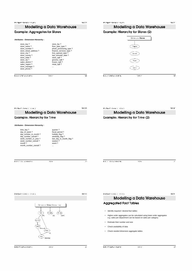
4 5 6 7 8 9 : V " ! 6 ! = F > S < ! ^ " 7
Attrib utes - Dimension Hierar chy :
time_key ? quarter ?day_of_week ? fiscal_period ?day_number_in_month ? holiday_flag ?day_number_overall ? weekday_flag ?week_number_in_year ? last_day_in_month_flag ?week_number_overall ? season ?month ? event ?month_number_overall ? ...
$ % & ' ( ( ) * + , - , . , / , 0 ' 1 % 2 3 '
� � � � � � � � � � � � � � � � � � � � � � � � � � � � D �
� � � � � � � � � � � � � � � � � � � � � � � � � � � � � � � � � �
4 5 6 7 8 9 : V " ! 6 ! = F > S < ! ^ " 7 P Q R$ % & ' ( ( ) * + , - , . , / , 0 ' 1 % 2 3 '
� � � � � � � � � � � � � � � � � � � � � � � � � � � � D A
� � � � � � � � � � � � � � � � � � � � � � � � � � � � � � � � � �
� � � � � � � � � � � � � � � � � � � � � � � � � � � � D D
� � � � � � � � � � � � � � � � � � � � � � � � � � � � � � � � � �
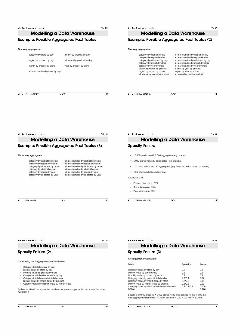
Z T T ! T 6 @ K W 6 = @ ^ 6 ] 9 C
• Identify required / desired fact tables
• Higher-order aggregates can be calculated using lower-order aggregatese.g. sales per department can be based on sales per category
• Estimate their number and size
• Check availability of data
• Check needed dimension aggregate tables
$ % & ' ( ( ) * + , - , . , / , 0 ' 1 % 2 3 '
� � � � � � � � � � � � � � � � � � � � � � � � � � � � D L
� � � � � � � � � � � � � � � � � � � � � � � � � � � � � � � � � �
4 5 6 7 8 9 : g K H @ " S > " H T Z T T ! T 6 @ K W 6 = @ ^ 6 ] 9 C
Desired aggregate fact tables:
• One-way aggregate: category totals by store by day
• One-way aggregate: district totals by store by day
• One-way aggregate: monthly totals by product by store
• Two-way aggregate: category totals by district totals by day
• Two-way aggregate: category totals by month totals by store
• Two-way aggregate: district totals by month totals by product
• Three-way aggregate: category totals by district totals by month totals
$ % & ' ( ( ) * + , - , . , / , 0 ' 1 % 2 3 '
� � � � � � � � � � � � � � � � � � � � � � � � � � � � D M
� � � � � � � � � � � � � � � � � � � � � � � � � � � � � � � � � �
4 5 6 7 8 9 : g K H @ " S > " H T Z T T ! T 6 @ K W 6 = @ ^ 6 ] 9 C
• 7 aggregated fact tables
• Aggregated fact tables are derivatives of basic fact table
• Checking additivity of fact table attributes:dollar_sales ?units_sales ?dollar_cost ?customer_count ?
• Aggregates of customer_count must be created at POS (point of sales)
$ % & ' ( ( ) * + , - , . , / , 0 ' 1 % 2 3 '
� � � � � � � � � � � � � � � � � � � � � � � � � � � � D N
� � � � � � � � � � � � � � � � � � � � � � � � � � � � � � � � � �
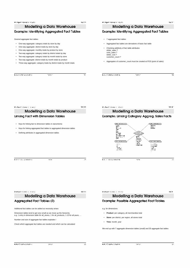
Y " H b " H T W 6 = @ # " @ F U " 7 H C " < H ^ 6 ] 9 C
• Keys for linking fact to dimension tables in starschema
• Keys for linking aggregated fact tables to aggregated dimension tables
• Defining attributes in aggregated dimension tables
$ % & ' ( ( ) * + , - , . , / , 0 ' 1 % 2 3 '
� � � � � � � � � � � � � � � � � � � � � � � � � � � � D O
� � � � � � � � � � � � � � � � � � � � � � � � � � � � � � � � � �
4 5 6 7 8 9 : Y " H b " H T \ 6 @ T < ! > Z T T ! T a ? 6 9 C W 6 = @ C$ % & ' ( ( ) * + , - , . , / , 0 ' 1 % 2 3 '
� � � � � � � � � � � � � � � � � � � � � � � � � � � � D �
� � � � � � � � � � � � � � � � � � � � � � � � � � � � � � � � � �
Z T T ! T 6 @ K W 6 = @ ^ 6 ] 9 C P Q R
Additional fact tables can be added as necessity arises
Dimension tables tend to get very small as we move up the hierarchye.g. 1 entry in dimension table for all_stores, 1 for all_products, 1-10 for all years, ...
Number and size of aggregate fact tables explodes !
Check which aggregate fact tables are needed and which can be calculated
$ % & ' ( ( ) * + , - , . , / , 0 ' 1 % 2 3 '
� � � � � � � � � � � � � � � � � � � � � � � � � � � � D �
� � � � � � � � � � � � � � � � � � � � � � � � � � � � � � � � � �
4 5 6 7 8 9 : I < C C " ] 9 Z T T ! T 6 @ K W 6 = @ ^ 6 ] 9 C
e.g. for dimensions
• Product : per category, all merchandise total
• Store : per district, per region, all stores total
• Time : month, year
We end up with 7 aggregate dimension tables (small) and 35 aggregate fact tables
$ % & ' ( ( ) * + , - , . , / , 0 ' 1 % 2 3 '
� � � � � � � � � � � � � � � � � � � � � � � � � � � � L �
� � � � � � � � � � � � � � � � � � � � � � � � � � � � � � � � � �
4 5 6 7 8 9 : I < C C " ] 9 Z T T ! T 6 @ K W 6 = @ ^ 6 ] 9 C
One way aggregates:
category by store by day district by product by day
region by product by day all stores by product by day
month by product by store year by product by store
all merchandise by store by day
$ % & ' ( ( ) * + , - , . , / , 0 ' 1 % 2 3 '
� � � � � � � � � � � � � � � � � � � � � � � � � � � � L �
� � � � � � � � � � � � � � � � � � � � � � � � � � � � � � � � � �
4 5 6 7 8 9 : I < C C " ] 9 Z T T ! T 6 @ K W 6 = @ ^ 6 ] 9 C P Q R
Two way aggregates:
category by district by day all merchandise by district by daycategory by region by day all merchandise by region by daycategory by all stores by day all merchandise by all stores by daycategory by month by store all merchandise by month by storecategory by year by store all merchandise by year by storedistrict by month by product district by year by productregion by month by product region by year by productall stores by month by product all stores by year by product
$ % & ' ( ( ) * + , - , . , / , 0 ' 1 % 2 3 '
� � � � � � � � � � � � � � � � � � � � � � � � � � � � L A
� � � � � � � � � � � � � � � � � � � � � � � � � � � � � � � � � �
4 5 6 7 8 9 : I < C C " ] 9 Z T T ! T 6 @ K W 6 = @ ^ 6 ] 9 C P _ R
Three wa y aggregates:
category by district by month all merchandise by district by monthcategory by region by month all merchandise by region by monthcategory by all stores by month all merchandise by all stores by monthcategory by district by year all merchandise by district by yearcategory by region by year all merchandise by region by yearcategory by all stores by year all merchandise by all stores by year
$ % & ' ( ( ) * + , - , . , / , 0 ' 1 % 2 3 '
� � � � � � � � � � � � � � � � � � � � � � � � � � � � L D
� � � � � � � � � � � � � � � � � � � � � � � � � � � � � � � � � �
? 8 6 ! C " @ > W 6 " 9 G !
• 10.000 products with 2.000 aggregates (e.g. brands)
• 1.000 stores with 100 aggregates (e.g. districts)
• 100 time periods with 30 aggregates (e.g. financial period based on weeks)
• 10% of all products sold per day
Additional size
• Product dimension: 20%
• Store dimension: 10%
• Time dimension: 30%
$ % & ' ( ( ) * + , - , . , / , 0 ' 1 % 2 3 '
� � � � � � � � � � � � � � � � � � � � � � � � � � � � L L
� � � � � � � � � � � � � � � � � � � � � � � � � � � � � � � � � �
? 8 6 ! C " @ > W 6 " 9 G ! P Q R
Considering the 7 aggregates identified before:
• Category totals by store by day• District totals by store by day• Monthly totals by product by store• Category totals by district totals by day• Category totals by month totals by store• District totals by month totals by product• Category totals by district totals by month totals
By how much will the size of the database increase as opposed to the size of the basefact table ?
$ % & ' ( ( ) * + , - , . , / , 0 ' 1 % 2 3 '
� � � � � � � � � � � � � � � � � � � � � � � � � � � � L M
� � � � � � � � � � � � � � � � � � � � � � � � � � � � � � � � � �
? 8 6 ! C " @ > W 6 " 9 G ! P _ R
A sug gestion / estimation:
Table Sparsity Factor
Category totals by store by day 0.2 0.2District totals by store by day 0.1 0.1Monthly totals by product by store 0.3 0.3Category totals by district totals by day 0.2*0.1 0.02Category totals by month totals by store 0.2*0.3 0.06District totals by month totals by product 0.1*0.3 0.03Category totals by district totals by month totals 0.2*0.1*0.3 0.006TOTAL 0.716
Baseline: 10.000 products * 1.000 stores * 100 time periods * 10% -> 100 mil.Plus aggregated fact tables: ~72% of baseline = 0.72 * 100 mil. -> 172 mil.
$ % & ' ( ( ) * + , - , . , / , 0 ' 1 % 2 3 '

� � � � � � � � � � � � � � � � � � � � � � � � � � � � L N
� � � � � � � � � � � � � � � � � � � � � � � � � � � � � � � � � �
? 8 6 ! C " @ > W 6 " 9 G ! P ` R
e.g. brands total by store by day:
• Assumption: only 10% of all products sold in given store on a given day ->10% of 10.000 products = 1.000 products being sold ->1.000 products in daily store data
• If every product sold belongs to a different brand ->1.000 different brands = 50%
• There may be 50% of all brands in the daily store data as opposed to 10% of theindividual products ->1.000 brands in daily store data
• Aggregated fact table may have same size as basic fact table
$ % & ' ( ( ) * + , - , . , / , 0 ' 1 % 2 3 '
� � � � � � � � � � � � � � � � � � � � � � � � � � � � L O
� � � � � � � � � � � � � � � � � � � � � � � � � � � � � � � � � �
? 8 6 ! C " @ > W 6 " 9 G ! P c R
Table Product Store Time Sparsity # Recor ds
Base: Products by store by week 10.000 1.000 100 10% 100 mil.Brand by store by week 2.000 1.000 100 50% 100 mil.Product by district by week 10.000 100 100 50% 50 mil.Product by store by period 10.000 1.000 30 50% 150 mil.Brand by district by week 2.000 100 80 80% 16 mil.brand by store by period 2.000 1.000 30 80% 48 mil.Product by district by period 10.000 100 30 80% 24 mil.Brand by district by period 2.000 100 30 100% 6 mil.
TOTAL 494 mill.
Database may grow up 394% !
$ % & ' ( ( ) * + , - , . , / , 0 ' 1 % 2 3 '
� � � � � � � � � � � � � � � � � � � � � � � � � � � � L �
� � � � � � � � � � � � � � � � � � � � � � � � � � � � � � � � � �
? 8 6 ! C " @ > W 6 " 9 G ! P d R
• Take care when designing aggregate tables
• Make sure that each aggregate summarizes at least about 10 - 20 records on theaverage
Example:
• Product dimension summarized only 5 lower level products on the average• Time dimension summarized only about 3 periods on the average• One way aggregates of time and product contributed 250 mil. records
• If each had summarized about 20 lower level items on average ->only about 70 mil. new records even with sparsity growing to 70%
$ % & ' ( ( ) * + , - , . , / , 0 ' 1 % 2 3 '
� � � � � � � � � � � � � � � � � � � � � � � � � � � � L �
� � � � � � � � � � � � � � � � � � � � � � � � � � � � � � � � � �
i G ! > " H T Z T T ! T 6 @ ^ 6 ] 9 C
Queries transformed into SQL statements
e.g.: Show total sales by category in Cincinnati stores on New Year’s Day 1998 for basefact table::
select category_description, sum(sales_dolars)from base_sales_fact, product, store, timewhere base_sales_fact.product_key = product.product_keyand base_sales_fact.store_key=store.store_keyand base_sales_fact.time_key = time.time_keyand store.city = ‘Cincinnati’and time.day = ‘January 1, 1996’group by category_description
$ % & ' ( ( ) * + , - , . , / , 0 ' 1 % 2 3 '
� � � � � � � � � � � � � � � � � � � � � � � � � � � � M �
� � � � � � � � � � � � � � � � � � � � � � � � � � � � � � � � � �
i G ! > " H T Z T T ! T 6 @ ^ 6 ] 9 C P Q R
Same query if category totals aggregate table exists:
select category_description, sum(sales_dolars)from category_sales_fact, category_product, store, timewhere category_sales_fact.product_key = category_product.product_keyand category_sales_fact.store_key=store.store_keyand category_sales_fact.time_key = time.time_keyand store.city = ‘Cincinnati’and time.day = ‘January 1, 1996’group by category_description
Category_sales_fact and corresponding category_product dimension table replace basesales fact and basic product dimension table
$ % & ' ( ( ) * + , - , . , / , 0 ' 1 % 2 3 '
� � � � � � � � � � � � � � � � � � � � � � � � � � � � M �
� � � � � � � � � � � � � � � � � � � � � � � � � � � � � � � � � �
i G ! > " H T Z T T ! T 6 @ ^ 6 ] 9 C P _ R
• Navigator
• Reads users query and transforms it into best available aggregate query
• Metadata descriptions provide information about existing aggregate tables
• Existence of aggregate tables is transparent to the user
• Can be used to build statistics on user queries, aggregate table usage and the needfor additional aggregates
• Allows incremental rollout of new aggregation tables
$ % & ' ( ( ) * + , - , . , / , 0 ' 1 % 2 3 '

� � � � � � � � � � � � � � � � � � � � � � � � � � � � M A
� � � � � � � � � � � � � � � � � � � � � � � � � � � � � � � � � �
i G ! > " H T Z T T ! T 6 @ ^ 6 ] 9 C P ` R
• Navigator: Replacing base-level fact and dimension tables with aggregated fact anddimension tables
1.) Rank order all aggregate tables
2.) Starting from the smallest, verify whether all of the dimensional attributes in the querycan be found.If so, replace base tables in query with corresponding aggregate tables.If not continue with the next bigger aggregate table until finally reaching the base facttable
$ % & ' ( ( ) * + , - , . , / , 0 ' 1 % 2 3 '
� � � � � � � � � � � � � � � � � � � � � � � � � � � � M D
� � � � � � � � � � � � � � � � � � � � � � � � � � � � � � � � � �
4 5 6 7 8 9 : j 6 � " T 6 @ < !$ % & ' ( ( ) * + , - , . , / , 0 ' 1 % 2 3 '
� � � � � � � � � � � � � � � � � � � � � � � � � � � � M L
� � � � � � � � � � � � � � � � � � � � � � � � � � � � � � � � � �
J @ 6 K 6 @ 6
• Describes the data in the DWH
• Technical metadata
• Business metadata
• Operational metadata
$ % & ' ( ( ) * + , - , . , / , 0 ' 1 % 2 3 '
� � � � � � � � � � � � � � � � � � � � � � � � � � � � M M
� � � � � � � � � � � � � � � � � � � � � � � � � � � � � � � � � �
4 5 6 7 8 9 : J @ 6 K 6 @ 6 W 6 = @ ^ 6 ] 9 $ % & ' ( ( ) * + , - , . , / , 0 ' 1 % 2 3 '
� � � � � � � � � � � � � � � � � � � � � � � � � � � � M N
� � � � � � � � � � � � � � � � � � � � � � � � � � � � � � � � � �
4 5 6 7 8 9 : J @ 6 K 6 @ 6 [ Z @ @ ! " ] G @ C$ % & ' ( ( ) * + , - , . , / , 0 ' 1 % 2 3 '
� � � � � � � � � � � � � � � � � � � � � � � � � � � � M O
� � � � � � � � � � � � � � � � � � � � � � � � � � � � � � � � � �
4 5 6 7 8 9 : J @ 6 K 6 @ 6 [ U ! " � K Z @ @ ! " ] G @ C$ % & ' ( ( ) * + , - , . , / , 0 ' 1 % 2 3 '

� � � � � � � � � � � � � � � � � � � � � � � � � � � � M �
� � � � � � � � � � � � � � � � � � � � � � � � � � � � � � � � � �
4 5 6 7 8 9 : J @ 6 K 6 @ 6 [ U " 7 H C " < H C$ % & ' ( ( ) * + , - , . , / , 0 ' 1 % 2 3 '
� � � � � � � � � � � � � � � � � � � � � � � � � � � � M �
� � � � � � � � � � � � � � � � � � � � � � � � � � � � � � � � � �
4 5 6 7 8 9 : J @ 6 K 6 @ 6 [ U " 7 H C " < H V " ! 6 ! = F " C$ % & ' ( ( ) * + , - , . , / , 0 ' 1 % 2 3 '
� � � � � � � � � � � � � � � � � � � � � � � � � � � � N �
� � � � � � � � � � � � � � � � � � � � � � � � � � � � � � � � � �
4 5 6 7 8 9 : J @ 6 K 6 @ 6 [ ^ " 7 U " 7 H C " < H$ % & ' ( ( ) * + , - , . , / , 0 ' 1 % 2 3 '
� � � � � � � � � � � � � � � � � � � � � � � � � � � � N �
� � � � � � � � � � � � � � � � � � � � � � � � � � � � � � � � � �
4 5 6 7 8 9 : J @ 6 K 6 @ 6 [ 4 g ? I 6 T $ % & ' ( ( ) * + , - , . , / , 0 ' 1 % 2 3 '
� � � � � � � � � � � � � � � � � � � � � � � � � � � � N A
� � � � � � � � � � � � � � � � � � � � � � � � � � � � � � � � � �
4 5 = G @ " � g H S < ! 7 6 @ " < H ? > C @ 7 C
• Briefing books
• Tables
• Charts
$ % & ' ( ( ) * + , - , . , / , 0 ' 1 % 2 3 '
� � � � � � � � � � � � � � � � � � � � � � � � � � � � N D
� � � � � � � � � � � � � � � � � � � � � � � � � � � � � � � � � �
4 5 6 7 8 9 : B ! " S " H T B < < b$ % & ' ( ( ) * + , - , . , / , 0 ' 1 % 2 3 '

� � � � � � � � � � � � � � � � � � � � � � � � � � � � N L
� � � � � � � � � � � � � � � � � � � � � � � � � � � � � � � � � �
4 5 6 7 8 9 : ^ 6 ] 9 $ % & ' ( ( ) * + , - , . , / , 0 ' 1 % 2 3 '
� � � � � � � � � � � � � � � � � � � � � � � � � � � � N M
� � � � � � � � � � � � � � � � � � � � � � � � � � � � � � � � � �
4 5 6 7 8 9 : \ F 6 ! @$ % & ' ( ( ) * + , - , . , / , 0 ' 1 % 2 3 '
� � � � � � � � � � � � � � � � � � � � � � � � � � � � N N
� � � � � � � � � � � � � � � � � � � � � � � � � � � � � � � � � �
I " @ S 6 9 9 C
• Not knowing what you really want
• Thinking that DWH-design is the same as transactional DB design - a DWH is notsimply a big database!
• Loading the warehouse with data simply because it is available
• Underestimating the complexity of a DWH project
• Getting caught by technological gadgets
• Focusing on internal data and ignoring the use of external data
• Using data with overlapping or confusing definitions / semantics
• Believing performance and scalability promises
• Believing that once a DWH is running the work is done
$ % & ' ( ( ) * + , - , . , / , 0 ' 1 % 2 3 '