DYNAMIC ANALYSIS OF ARCH DAMS: EFFECT OF THERMAL LOADING

by

Ryhane Moghadas Jafari

A THESIS SUBMITTED IN PARTIAL FULFILLMENT OF

THE REQUIREMENTS FOR THE DEGREE OF

MASTER OF APPLIED SCIENCE

in

THE COLLEGE OF GRADUATE STUDIES

(Civil Engineering)

THE UNIVERSITY OF BRITISH COLUMBIA

(Okanagan)

January 2016

© Ryhane Moghadas Jafari, 2016

ii

Abstract

Conducting a case study, this thesis investigates the dynamic behavior of Karun IV arch dam

(Iran) under the effect of maximum feasible thermal input. A three-dimensional finite

element model is created using ANSYS software. The thesis determines the impact of

thermal loadings under two scenarios of normal and minimum water levels. The dam-

foundation, dam-water and water-foundation interactions are considered in the modeling to

accurately capture its dynamic response. Furthermore, in addition to the water

compressibility, appropriate wave absorbing boundaries are used for the reservoir far end and

bottom and for the foundation. Stability, static, modal, and thermal analyses are conducted as

initial conditions. Using three orthogonal earthquake components, linear dynamic time

history analyses with and without thermal loading are performed. The comparison of the

results verified that the application of thermal effects on the dynamic analysis increases the

maximum tension, changes the maximum pressure, and decreases the displacements in the

dam body. This study concludes that thermal loading must be considered in the dynamic

analysis of an arch dam as it can worsen the tensile cracks.

iii

Table of Contents

Abstract .................................................................................................................................... ii

Table of Contents ................................................................................................................... iii

List of Tables .......................................................................................................................... vi

List of Figures ........................................................................................................................ vii

List of Abbreviations ............................................................................................................. ix

List of Symbols ........................................................................................................................ x

Acknowledgements .............................................................................................................. xiii

Dedication ............................................................................................................................. xiv

Chapter 1 Introduction........................................................................................................... 1

1.1 Research Motivation ............................................................................................................. 1

1.2 Research Objective, Assumptions and Methodology ........................................................... 2

1.3 Thesis Outline ....................................................................................................................... 3

Chapter 2 Literature Review ................................................................................................. 4

2.1 Seismic Failure Mechanisms of Arch Dams and Their Affecting Factors............................ 4

2.2 Necessity of Seismic Analysis of Arch Dams ....................................................................... 5

2.3 Thermal Loading in Safety Analysis of Arch Dams ............................................................. 5

2.4 Literature Review .................................................................................................................. 7

Chapter 3 Governing Equations and Boundary Conditions ............................................ 10

3.1 Damping .............................................................................................................................. 10

3.1.1 Material Damping Matrix ............................................................................................... 10

3.2 Finite Element Equation of the Dam Body ......................................................................... 11

3.3 Equation of Motion for the Reservoir ................................................................................. 11

3.4 Finite Element Equation of the Reservoir ........................................................................... 12

3.5 Dam-Reservoir Interaction .................................................................................................. 13

3.6 Finite Element Equation of the Coupled Dam-Reservoir ................................................... 13

3.6.1 Effect of Soil-Structure Interaction................................................................................. 13

3.6.2 Direct Method ................................................................................................................. 14

iv

3.7 Effect of Foundation Mass .................................................................................................. 15

3.8 Thermal Boundary Conditions ............................................................................................ 16

3.9 Reservoir Boundary Conditions .......................................................................................... 16

3.9.1 Reservoir Free Level Boundary Condition ..................................................................... 16

3.9.2 Dam-Reservoir Boundary Condition .............................................................................. 17

3.9.3 Reservoir-Foundation Boundary Condition .................................................................... 17

3.9.4 Far End of the Reservoir Boundary Condition ............................................................... 18

3.10 Semi-Infinite Foundation Boundary Condition .................................................................. 20

Chapter 4 Modeling of the Dam Body, Reservoir, and Foundation ................................ 21

4.1 Geometric Characteristics of the Dam ................................................................................ 21

4.1.1 Concrete Characteristics ................................................................................................. 21

4.2 Water Specifications ........................................................................................................... 24

4.3 Foundation Materials Specifications ................................................................................... 24

4.4 Specifications of the Finite Element Model of the Dam, Reservoir, and Foundation ........ 24

4.4.1 Finite Element Model of the Dam Body ......................................................................... 25

4.4.1.1 Solid45 Element ..................................................................................................... 26

4.4.1.2 Solid70 Element ..................................................................................................... 26

4.4.2 Finite Element Model of the Reservoir........................................................................... 26

4.4.2.1 Fluid30 Element ..................................................................................................... 27

4.4.3 Finite Element Model of the Foundation ........................................................................ 28

4.4.3.1 Combine14 Element ............................................................................................... 29

Chapter 5 Loadings, Analyses and Results......................................................................... 30

5.1 Types of Loading ................................................................................................................ 30

5.2 Seismic Loading .................................................................................................................. 30

5.2.1 Earthquake Frequency Content ....................................................................................... 31

5.2.2 Earthquake Duration ....................................................................................................... 31

5.3 Thermal Analysis ................................................................................................................ 36

5.4 Stability Analysis ................................................................................................................ 38

5.5 Static Analysis .................................................................................................................... 39

5.6 Modal Analysis ................................................................................................................... 41

5.7 Dynamic Analysis ............................................................................................................... 42

5.7.1 Dynamic Analysis without Thermal Loading ................................................................. 43

5.7.2 Dynamic Analysis with Thermal Loading ...................................................................... 50

v

Chapter 6 Conclusion ........................................................................................................... 58

6.1 Conclusions ......................................................................................................................... 58

6.2 Recommendations ............................................................................................................... 60

References .............................................................................................................................. 61

Appendix A: Permission Request ........................................................................................ 66

vi

List of Tables

Table 1 Basic information about the dam (Iran Water & Power Resources Development

Co., 2004) ............................................................................................................... 21

Table 2 Mechanical and thermal properties of the dam concrete (Iran Water & Power

Resources Development Co., 2004) ....................................................................... 23

Table 3 Natural vibration frequencies for the first fifteen vibration modes of the system .. 41

vii

List of Figures

Figure 1 Research overview ................................................................................................... 3

Figure 2 Heat sources and heat transfer processes of an arch dam (adopted from

Sheibany & Ghaemian, 2006, with permission from ASCE) ................................ 6

Figure 3 Complete model of the dam-reservoir-foundation ................................................ 24

Figure 4 Format of the finite element grid of the dam body ................................................ 25

Figure 5 Analytical model of the reservoir .......................................................................... 27

Figure 6 Analytical model of the foundation rock ............................................................... 29

Figure 7 X-direction record of the earthquake ..................................................................... 32

Figure 8 Y-direction record of the earthquake ..................................................................... 33

Figure 9 Z-direction record of the earthquake ..................................................................... 34

Figure 10 Fourier Transform Amplitude of X, Y, and Z components of the earthquake .... 35

Figure 11 Curve of the energy released during the earthquake for X component ............... 35

Figure 12 Thermal input in the crown cantilever................................................................. 36

Figure 13 Temperature distribution in the dam body for the summer and winter critical

times ..................................................................................................................... 37

Figure 14 Distribution of the maximum principal stress (S1) and minimum principal

stress (S3) for downstream and upstream faces in the stability analysis ............. 38

Figure 15 Distribution of the X direction displacement (m) in the stability analysis .......... 39

Figure 16 Distribution of S1 and S3 for upstream and downstream faces in static

analysis ................................................................................................................ 40

Figure 17 Distribution of X direction displacement (m) in static analysis .......................... 40

Figure 18 First seven vibration modes of the dam body ...................................................... 42

Figure 19 Nodes used for consideration of dynamic analyses results on the dam

upstream and downstream faces .......................................................................... 43

Figure 20 S1 and S3 distribution envelops for the dam upstream and downstream faces

in state (a) ............................................................................................................ 44

Figure 21 Time-history curve for the dam crest displacement in X direction in state (a) ... 45

Figure 22 Time-history curves of S1 for the selected nodes in the dam upstream face in

state (a) ................................................................................................................. 45

viii

Figure 23 Time-history curves of S1 for the selected nodes in the dam downstream face

in state (a) ............................................................................................................ 46

Figure 24 S1 and S3 distribution envelops for the dam upstream and downstream in state

(b) ......................................................................................................................... 47

Figure 25 Time-history curve for the dam crest displacement in X direction in state (b) ... 48

Figure 26 Time-history curves of S1 for the selected nodes in the dam upstream face in

state (b) ................................................................................................................ 48

Figure 27 Time-history curves of S1 for the selected nodes in the dam downstream face

in state (b) ............................................................................................................ 49

Figure 28 S1 and S3 distribution envelops for the dam upstream and downstream faces

in state (c) ............................................................................................................ 51

Figure 29 Time-history curve for the dam crest displacement in X direction in state (c) ... 52

Figure 30 Time-history curves of S1 for the selected nodes in the dam upstream face in

state (c) ................................................................................................................. 52

Figure 31 Time-history curves of S1 for the selected nodes in the dam upstream face in

state (c) ................................................................................................................. 53

Figure 32 S1 and S3 distribution envelops for the dam upstream and downstream faces

in state (d) ............................................................................................................ 54

Figure 33 Time-history curve for the dam crest displacement in X direction in state (d) ... 55

Figure 34 Time-history curves of S1 for the selected nodes in the dam upstream face in

state (d) ................................................................................................................ 55

Figure 35 Time-history curves of S1 for the selected nodes in the dam upstream face in

state (d) ................................................................................................................ 56

ix

List of Abbreviations

3D Three-Dimensional

FEM Finite Element Model

CEA Canadian Electricity Association

USACE U.S. Army Corps of Engineers

DBE Design Basis Earthquake

MCE Maximum Credible Earthquake

NWL Normal Water Level

MWL Minimum Water Level

PREF Reference pressure

x

List of Symbols

𝜌 Considered medium density

𝐶 Specific heat

𝑇 Temperature

{𝑉} Mass transport heat flow

∇ Divergence

∇° Gradient

𝑡 Time

[𝐷] Conductivity matrix

𝑣𝑜𝑙 Element volume

{𝑞} Thermal flux vector

𝑆2 Concrete dam exposed surfaces subject to thermal flows

𝑆3 Concrete dam exposed surfaces subject to convection

ℎ𝑓 Heat transfer coefficient

𝑇𝐵 Temperature of the adjacent fluid

𝑞 Heat production rate per unit volume

[𝑀] Mass matrix

[𝐶] Damping matrix

[𝐾] Stiffness matrix

𝛼 Mass coefficients matrix

𝛽 Stiffness coefficients matrix

𝑖, 𝑗 Dominant vibrational modes of the system

𝜉 Damping ratio

𝜔𝑖, 𝜔𝑗 ith

and jth

natural frequencies

𝜔 Frequency of dominant vibration mode of the system

{�̈�} Acceleration of the structural nodes relative to the ground

{�̇�} Nodal acceleration vector

{𝑈} Nodal displacement vector

{𝑓} Hydrodynamic pressure vector

xi

{𝑓1} Resultant vector of the other forces on the structure

{�̈�𝑔} Ground acceleration (earthquake) in the base of the structure

Ρ Fluid pressure

𝐶 Velocity of fluid pressure wave (sound wave)

𝐾 Bulk modulus

[𝐺] Reservoir mass matrix

{𝑃} Reservoir hydrodynamic pressure vector

[�́�] Damping matrix of the reservoir

[�́�] Reservoir stiffness matrix

{𝐹} Pseudo force vector in the fluid due to the boundary conditions in the

reservoir surfaces

[𝑄] Coupled matrix of the dam-reservoir interface which converts the

reservoir pressure into nodal forces on the structure

{𝐹𝐹1} Force vector related to the acceleration of the dam-reservoir and reservoir-

foundation

{𝐹2} Force vector due to the ground acceleration in the dam-reservoir boundary

and the total acceleration in the other boundaries

[𝐷] Conductivity matrix

[𝐻] Pseudo rigidity matrix

ℎ Reservoir depth

{𝐹1} Force vector of volumetric and hydrostatic forces

𝐶𝐿 Longitudinal wave speed in the foundation ambient

𝑎° Dimensionless frequency

𝑔 Acceleration of gravity

Ζ Vertical axis with the center at the water surface

n Perpendicular vector to the surface unit in the dam-reservoir interface

ans Dam structure acceleration along n vector

𝜌𝑟 Density of the materials in the reservoir bottom

𝐶𝑟 Longitudinal wave velocity in the reservoir bottom materials

𝐸𝑟 Modulus of elasticity of the reservoir bottom materials

xii

𝑎𝑛 (𝑡) Acceleration of the reservoir bottom in the time 𝑡

𝐸𝑐 Concrete modulus of elasticity

𝑓𝑐 90-day compressive strength of the concrete

𝑓𝑡 Tensile strength of the concrete

𝜐 Poisson’s ratio

𝛼 Coefficient of thermal expansion

𝐸𝑓 Deformation modulus of foundation rock mass

𝑆1 Maximum principal stress

𝑆3 Minimum principal stress

𝐷𝑆 Downstream face

𝑈𝑆 Upstream face

𝑈𝑥 Displacement of the dam crest in 𝑥 direction

xiii

Acknowledgements

I appreciate the efforts of my supervisor, Dr. Bahman Naser.

I owe special thanks to my parents because of their whole life supports and inspiring.

I thank the faculty, staff, and my fellow students at the UBCO, who encouraged me to

continue my work in this field.

xiv

Dedication

1

Chapter 1 Introduction

Dams play an important role in the optimal use of surface water resources in dry or semi-dry

countries, also for making clean hydropower energy in the world. Dam failure makes

disastrous life and property losses as it has been observed in the history. Therefore, structural

dam safety is very important and critical. A realistic consideration of all factors affecting

dam safety while designing new projects or updating safety evaluations of existing dams can

improve their efficient operation, particularly in arch dams. Comparing to the other dams

(e.g. gravity and rock fill dams) arch dams indicate a more complicated behavior due to their

three-dimensional thin arch structure, the mechanism of load transfer to the supports, and the

operation of contraction joints. According to statistics, arch dams display somewhat worse

performance over time compared to other type of dams (Regan, 2010). As various loading

conditions and interactions among different media (water, dam, foundation, and ambient

environment) may affect their performance more significantly, this dissertation focuses on

arch dams.

1.1 Research Motivation

Arch dams are under static, dynamic and thermal loadings. Static loads include the self-

weight and hydrostatic pressure. Dynamic loads include the impact force of the earthquake

on the structure and the hydrodynamic pressure of the water behind the dam.

Thermal effects have been reported as the main causes of the deterioration in concrete

dams. Freeze-thaw cycles covered 19% of cases, while temperature changes were 9% of

cases (ICOLD, 1984). In regions with high difference between seasonal ambient air

temperature, (e.g. in some areas in Canada the temperature changes between summer and

winter reaches to 45°C), the associated thermal stresses may go above the allowable tensile

strength of concrete and that may eventually cause tensile failures (Daoud et al., 1997).

Previous researchers and designers considered thermal input as a predetermined

assumption for their calculations. According to their point of view, arch dams are very

sensitive to the variation of ambient temperature due to their special geometries and shapes.

Therefore, temperature changes within the dam body and their related thermal stresses should

be included as initial conditions in any safety analysis of arch dams (Agullo et al., 1996;

2

Daoud et al., 1997; Sheibany & Ghaemian, 2006; Mirzabozorg et al., 2014). This research

tests and verifies the necessity of this assumption for the case of Karun IV arch dam (Iran).

This is done by creating an advanced three-dimensional (3D) finite element model (FEM) of

the dam.

1.2 Research Objective, Assumptions and Methodology

As overall objective, this study aims at investigating the significance of thermal loading on

the dynamic response of double curvature Karun IV arch dam. This objective is achieved

through the following sets of goals:

Stability Analysis: to verify dam stability under its weight;

Static Analyses: to study dam stability under full static loading conditions as well as

an initial condition for dynamic analyses;

Thermal Analyses: to find temperature distribution over the dam body;

Modal Analysis: to determine the natural mode shapes and frequencies of the dam;

and

Dynamic Analyses: to create a comprehensive dynamic response of the dam under all

loading conditions.

The following assumptions were adopted in this project:

The reservoir is modeled with normal and minimum and water levels;

Water is compressible;

Ignoring the hydration heat, the research studies only thermal loads due to ambient

temperature change;

Dynamic analysis considers horizontal as well as vertical components of earthquake;

Foundation is assumed to be massive;

Dam-reservoir, dam-foundation and reservoir-foundation interactions are considered;

and

Absorbing boundaries are located on the bottom, walls, and far end of the reservoir,

and around the foundation as well.

Figure 1 shows the steps for research methodology. A 3D FEM of the dam is provided by the

ANSYS software. Thermal, stability, static, and modal analyses are done as initial

3

conditions. Finally, linear dynamic time-history analyses, without and with thermal loading,

are performed and the results are compared.

Figure 1 Research overview

1.3 Thesis Outline

This research is reported in six chapters. Chapter 1 is an introduction to the research problem.

Chapter 2 briefly reviews the relevant background and literature. Chapter 3 explains briefly

about governing equations and boundary conditions of the model. The characteristics of the

FEM of the dam body, reservoir, and foundation are discussed in Chapter 4. Chapter 5

presents loading conditions and provides the analyses scenarios and their results. Chapter 6

concludes the thesis by highlighting the key findings and recommending future research.

4

Chapter 2 Literature Review

2.1 Seismic Failure Mechanisms of Arch Dams and Their Affecting Factors

According to the previous observations and experiences, the probable mechanism of damage

of an arch dam under the earthquake can be classified as follows:

1- Under seismic loads, tensile stresses in some points of the dam body exceed

the limit, making cracks in those points. Vertical joints are made of lower resistance

materials compared to the concrete. Therefore, due to an increase in the tensile stresses, the

vertical joints between the blocks and also the horizontal seams open. This problem leads to

the loss of integrity of the dam body and changes the force transmission system from arch to

cantilever. If the cracked blocks do not withstand additional loads, they will break and result

in the general or partial damage of the dam.

2- Sliding of the masses around the valley and over the reservoir on the dam

body, sliding of the masses over the reservoir into the reservoir, and mud displacement

beneath the reservoir can create damage in part of the dam or powerful waves in the

reservoir. These waves can subsequently result in the overflow of the reservoir water on the

dam crest, overpass, destruction of the spillways and the side structures, and ultimately the

destruction of the dam.

3- Earthquake can cause displacement of the fault, landslide or cracks in the

stony foundation of the dam. These can cause probable damage in the grout curtain, which

causes an increase in water leakage and in pore-water pressure in foundation. Eventually, the

problems in the foundation lead to the dam slide and damage (Tatalovich, 1998).

Some of the factors that influence the seismic response of an arch dam are as follows

(Zhou et al., 2000):

Characteristics and intensity of the earthquake, waveforms, and vibration modes, and

their changes.

Interaction of the dam body with the foundation material and the reservoir water;

interaction of the foundation with the reservoir water.

Features of the existing materials; changes in the features of dam materials (material

nonlinearity).

Cracking or opening-closing of cracks in the dam body, foundation and joints; relative

5

displacement of vertical or horizontal joints of the dam body; joint sliding and

compression (geometric nonlinearity).

Type of computer modeling (in terms of meshing and other characteristics), and

Reservoir water level.

2.2 Necessity of Seismic Analysis of Arch Dams

Because of severity and intensity of dynamic forces, dynamic analysis and design of arch

dams are essential. According to the statistic declared by CEA (Canadian Electricity

Association) in 1990, USACE (U.S. Army Corps of Engineers, 1995), and Knight and Mason

(1992), many arch concrete dams were affected by severe earthquakes such as Pacoima and

Hoover (United States), Kurobe (Japan), Monteynard (France), Maina Sarris (Italy), Kariba

(Zimbabwe), and Rapel (Chile). Among them, Rapel and Pacoima dams were damaged

(Tinawi et al., 2000). Furthermore, according to the statistics declared by Serafim and

Olivera regarding the information collected since 1987 to 1994 from 1527 existing dams, 42

dams were subjected to earthquake and 8 dams were damaged (Serafim & Oliveira, 1987).

The mentioned statistics and studies have indicated that the previous design methods,

contrary to the expectations, have not been conservative. It should be taken into

consideration that due to the long return period for large earthquakes, many of the existing

dams in the areas of high seismicity have not experienced yet the predicted earthquakes by

the seismicity studies. Therefore, the catastrophic losses due to the failure of dams indicate

the importance of updated seismic analysis for arch dams and re-examination of the behavior

of these structures. It should be done through using up-to-date computational models and

analysis techniques, and consequently evaluating the stress response, resistance, and

movement of dam-reservoir-foundation system as well.

2.3 Thermal Loading in Safety Analysis of Arch Dams

Arch dams are thin, arched and fixed in foundation and abutments. This special condition

makes them sensitive to the variation of the ambient temperature. Figure 2 shows the general

heat sources and thermal boundary conditions in the operational phase of an arch dam. The

boundary conditions at the interface of concrete and air are solar radiation, concrete-air

convection, and concrete radiation to the air (Sheibany & Ghaemian, 2006). Air and water

6

temperature are obtained from meteorological reports. The concrete and water temperature

are the same at the concrete and water interface (Sheibany & Ghaemian, 2006).

Figure 2 Heat sources and heat transfer processes of an arch dam (adopted from Sheibany & Ghaemian,

2006, with permission from ASCE)

Heat transfer is taken into consideration in construction as well as operational phases

of a concrete dam (U. S. Army Corps of Engineers, 1994; Sheibany & Ghaemian, 2006; Li et

al., 2014). Heat of operation is also considered at least from two aspects; first, the effects of

long term changes in the ambient temperature and second, the effects of temperature

distribution in the dam body at certain times (i.e., after the peak of summer heat and the peak

of winter cold).

Regarding the first aspect, according to literature, stresses caused by annual

temperature variation have a significant effect on reducing the strength and durability of arch

dams throughout the year, especially in the areas with high thermal gradients. Moreover, the

thermal response of concrete dams affects some properties of concrete mixture such as creep,

thermo-elastic properties and alkali aggregate reactions (Sheibany & Ghaemian, 2006; Li et

al., 2014).

Thermal cracks are not directly responsible for the instability of arch dams. Rather,

due to the weathering, water and sediments penetration, and the permanent cycles of melting-

7

freezing, the cracks gradually broaden and cause more destruction in the dam concrete.

Therefore, an aged-dam affected by an earthquake at a specific moment has initial stress

distribution due to the heat and also a series of thermal cracking and demolition.

Consequently, earthquake and hydrodynamic forces exerted on the dam, together with

already existing gravity and hydrostatic loads, can extend cracks and cause general instability

of the dam (Javanmardi et al., 2005).

2.4 Literature Review

In the realm of investigating temperature distribution and thermal effects on dams, Agullo

and Aguado (1995) proposed a one-dimensional simple explicit finite-difference scheme by

developing a simple analytical formula. This simple model predicted the thermal behavior of

the dam body based on the dam height, at various sections for different given heights and

changeable thicknesses, at any moment. The scheme considered concrete thermal variables,

dam site and geometry, as well as environmental function of the dam. According to their

research, annual mean temperature of the ambient, water, and the total daily solar radiation at

the site, mainly influences the mean temperature of the section. The section thickness, annual

range of the ambient and water temperatures affects the annual range of the mean

temperature of the desired section. Between all those stimuli, the solar radiation mainly

affects the temperature of each layer.

An analytical method using unidirectional heat transfer was proposed by Zhang and

Gargaa (1996). This model determined the temperature distribution for the thermal shock

scenarios happening on mass concrete structures. By making an analytical formula based on

superposition method for sinusoidal and triangular air temperature loading, the most

temperature gradient and consequently stresses were observed near the exposed surface in a

narrow area. They found the concrete properties and the coefficient of heat transfer should be

changed to reduce the stress concentration.

Meyer and Mouvet (1995) made a three-dimensional finite element model for Vieux–

Emosson arch-gravity dam in Switzerland. Using the numerical analysis, they calculated the

temperature gradients and consequent thermal stresses, strains, and displacements. They

divided the downstream face into three areas and gave each area a different absorption of

solar radiation. According to their results, which were not compatible with obtained

8

instrumental data, the thermal expansion coefficient has an important role on the

deformability of the dam while the rock and the concrete module of elasticity are not

significant.

Leger et al. (1993) carried out a two-dimensionally modeled numerical analysis for

finding the temperature-affected area in a concrete gravity dam with the assumptions of no

horizontal heat transfer and similar boundary conditions for different cross sections. Because

of the plain and non-concave downstream surface of the gravity dams, there is no change in

the solar radiation exposure. According to the results, the temperature gradient is created

close to the exposed surface resulting in the tensile stresses. The consequent surface cracks

are harmful just because of freezing and thawing cycles of penetrated water, but do not make

the dam instable.

Daoud et al. (1997) proposed a somehow comprehensive two-dimensional finite

element numerical analysis for gravity dams with periodic temperature field. They

considered the assumptions of past researchers including solar radiation, air temperature

variations, temperature gradients, as well as their own new ones including snow cover,

reservoir ice formation, and conductivity change in the saturated part and unsaturated part of

the dam. According to their observations, despite of a change in the related thermal

conductivities by just 8%, temperature gradient varies significantly along with the interface

of the saturated and unsaturated parts. Furthermore, they found thermal degradation happens

nearly in 1 meter region from the open surface of the downstream.

Besides Leger et al. (1993) and Daoud et al. (1997), who made a simplified variation

pattern of the temperature profile of the reservoir, Bofang (1997) also suggested a boundary

condition of water temperature variations for deep reservoirs of concrete dams using an

analytical formula (Mirzabozorg & Varmazyari, 2009).

Sheibany and ghaemian (2006) predicted the thermal gradient and the consequent

thermal stress distribution in the operational phase of an arch dam. They made a three-

dimensional finite element model and considered experimentally realistic air temperature and

additional assumptions including experimentally realistic reservoir temperature and the

changing share of solar radiation over the exposed surface of the dam. They applied the

effects of diffuse and beam radiation, surface azimuth, sun declination, surface slope,

latitude, and the water and ground reflectivity. They did not consider the foundation

9

temperature in the model. They neglected the effect of temperature on the mechanical and

thermal properties of the concrete. The thermal properties were considered uniform and

isotropic. The hydration heat of cement after construction was not applied. At the concrete-

air interface, solar radiation, concrete-air convection, and concrete radiation to the air were

the assumed boundary conditions. At the concrete-water interface, no convection and

radiation, and as a result, similar water and concrete temperature were considered.

Mirzabozorg et al. (2014) considered the solar radiation, air, and water temperature

effects on the thermal analysis of dams with finite element modeling methods. Wang et al.

(2011) made a thermal dynamic analysis of a concrete gravity dam using a three-dimensional

finite element model, the application of iteration method, and cooling pipe discrete. They

analyzed the transient temperature field and their distributions. They used sensible

temperature control measures as reference. Their suggested temperature control measures

effectively resulted into controlling the temperature and preventing the cracks.

Hariri-Ardebili & Kianoush (2014) presented an integrative nonlinear seismic safety

analysis of a calibrated model of a high arch dam. They carried out a static and thermal

calibration procedure, followed by a nonlinear dynamic analysis on the resulted model. From

the assumption side, their research was realistic as they considered mass concrete cracking,

geometric nonlinearity, joint opening and closing, the effect of water pressure and

penetration inside the joints. According to their findings, the loaded dam extensively cracked

and joints slid under the applied assumptions.

Liu et al. (2015) also considered thermal effects in the mass concrete in the presence

of a pipe cooling system. They made a heat-fluid coupling model and analyzed a high arch

dam monolith with that during the construction period. They considered different factors

including thermal characteristics of the material, cooling pipe system and schedule, and real

climate condition. They found this method effective on modeling the thermal field of

complex mass concrete structures including cooling pipe systems.

10

Chapter 3 Governing Equations and Boundary Conditions

This chapter explains the relevant governing equations used by the software to model the

thermal and seismic analysis, considering dam-foundation-reservoir interactions, and the

boundary conditions for those in an arch dam.

3.1 Damping

Damping has an important effect on dynamic response of arch dams and includes material

damping (viscous damping), frictional damping (Coulomb), and radiation damping

(geometric). The associated energy loss originates from different sources including concrete

arch structure, foundation rock and reservoir water. Energy dissipation in the arch structure is

due to the internal friction of concrete materials and construction joints (frictional damping).

The factors which cause earthquake energy loss in the foundation rock are expansion of the

elastic waves from the dam body to the distant in foundation (radiation damping) and the

hysteretic due to sliding of cracks and joints in the foundation rock (frictional damping). In

the reservoir, diffraction of hydrodynamic pressure waves into the reservoir bottom material

and expansion of pressure waves toward the reservoir upstream (radiation damping) create

damping (U. S. Army Corps of Engineers, 1994).

3.1.1 Material Damping Matrix

The seismic response of arch dams is determined based on linear elastic dynamic analysis.

The dynamic analysis of the present model is made in time history analysis method. The

direct integration model is used by software for step-by-step numerical integration in order to

solve equations of motion. In direct integration method, it is necessary to determine explicit

damping matrix. Rayleigh damping method is employed to create the damping matrix

(Chopra, 1967):

[𝐶] = 𝛼[𝑀] + 𝛽[𝐾] ‎3.1

where [𝑀] is the mass matrix, [𝐶] is the damping matrix, [𝐾] is the stiffness matrix, and

𝛼 and 𝛽 are the mass and stiffness coefficients matrices, respectively. They can be written as:

11

{

𝛼 = 𝜉

2𝜔𝑖𝜔𝑗

𝜔𝑖 + 𝜔𝑗

𝛽 = 𝜉2

𝜔𝑖 + 𝜔𝑗

‎3.2

where 𝑖 and 𝑗 are the dominant vibrational modes of the system, 𝜉 is the damping ratio,

𝜔𝑖 𝑎𝑛𝑑 𝜔𝑗 are the ith

and jth

natural frequencies. After determination of 𝛼 and 𝛽, damping

matrix can be determined by the above equation (Chopra, 1967). Because of the severe and

complicated effect of mass matrix coefficient on the response of dam-reservoir-foundation

system in arch dams, 𝛼 is considered zero. Therefore, damping matrix and stiffness matrix

coefficient is calculated as follows:

[𝐶] = 𝛽[𝐾] ‎3.3

𝛽 = 𝜉 (2

𝜔) ‎3.4

where 𝜔 is the frequency of dominant vibration mode of the system (Chopra, 1967).

3.2 Finite Element Equation of the Dam Body

During an earthquake, dam body is modeled as a Multi-Degree-of-Freedom (MDF) system.

To stimulate the earthquake in all directions, we will have:

[𝑀]{�̈�} + [𝐶]{�̇�} + [𝐾]{𝑈} = {𝑓} + {𝑓1} − [𝑀]{�̈�𝑔} ‎3.5

where {�̈�} is the acceleration of the structural nodes relative to the ground, {�̇�} is the nodal

acceleration vector, {𝑈} is the nodal displacement vector, {𝑓} is the hydrodynamic pressure

vector, {𝑓1} is the resultant of the other forces on the structure, and {�̈�𝑔} is the ground

acceleration (earthquake) in the base of the structure. This equation is the final finite element

form of the equation of motion for the dam body (Ghaemian & Ghobarah, 1999).

3.3 Equation of Motion for the Reservoir

By placing Stoke’s Viscosity Low in the linear momentum equation for a Newtonian fluid,

with the assumption of constant density and viscosity of the fluid, the small amplitude

motion for the reservoir, linear and non-rotational compressible fluid, and the application of

12

the continuity equation, the final equation for the reservoir is obtained as follows (White &

Corfield, 2006):

𝛻2𝑃 =1

𝐶2𝜕2𝑃

𝜕𝑡2 ‎3.6

where Ρ is fluid pressure, 𝐶 = √𝐾 𝜌⁄ is the velocity of fluid pressure wave (sound wave),

𝐾 is called bulk modulus, and 𝜌 is the water density. Given the fluid compressibility, the

amount of added mass and the energy loss caused by fluid during earthquake change in the

time domain. Therefore, there will be more coordination between the actual behavior of the

dam and mathematical models (DeSalvo & Swanson, 2006).

3.4 Finite Element Equation of the Reservoir

By application of the obtained boundary condition for the reservoir and weak Galerkin

method, the final equation used by the software is:

[𝐺]{�̈�} + [�́�]{�̇�} + [�́�]{𝑃} = {𝐹} − 𝜌[𝑄]𝑇({�̈�𝑔} + {�̈�}) = {𝐹𝐹1}

= {𝐹2} − 𝜌[𝑄]𝑇{�̈�}

‎3.7

and:

|[�́�] =

[𝐷]

𝐶

[�́�] = [𝐻] +𝜋

2ℎ[𝐷]

‎3.8

where [𝐺] is the reservoir mass matrix, {𝑃} is the reservoir hydrodynamic pressure vector,

[�́�] is the damping matrix of the reservoir, [�́�] is the reservoir stiffness matrix, {𝐹} is the

pseudo force vector in the fluid due to the boundary conditions in the reservoir surfaces, 𝜌 is

the water density, [𝑄] is the coupled matrix of the dam-reservoir interface which converts the

reservoir pressure into nodal forces on the structure, {𝐹𝐹1} is the force component related to

the acceleration of the dam-reservoir and reservoir-foundation, {𝐹2} vector represents the

forces due to the ground acceleration in the dam-reservoir boundary and the total acceleration

in the other boundaries, [𝐷] is the conductivity matrix, [𝐻] is the pseudo rigidity matrix, and

ℎ is the reservoir depth (Ghaemian & Ghobarah, 1999; DeSalvo & Swanson, 2006).

13

3.5 Dam-Reservoir Interaction

During an earthquake, the main loading factor on the dam structure is the inertia exerted on

the upstream face of the dam which stems from earth movement and the hydrodynamic force

of the reservoir fluid. Because of the seismic motion of the abutments around the reservoir,

the pressure waves created by the earthquakes, which travel to the reservoir upstream,

remove part of the kinetic energy of the system from the environment. In addition, the

deformations or vibrations of the dam body during earthquake affect the hydrodynamic

pressures created in the fluid adjacent to the dam body (Chopra, 1967). Therefore, from the

above, it can be concluded that the temporal response of both the dam and the reservoir

subsystems are dependent to each other and must be assessed simultaneously (U. S. Army

Corps of Engineers, 2003).

3.6 Finite Element Equation of the Coupled Dam-Reservoir

According to the equations for the dam body and the reservoir, the coupled equation for the

dam-reservoir can be written as follows (Ghaemian & Ghobarah, 1999):

|[𝑀]{�̈�} + [𝐶]{�̇�} + [𝐾]{𝑈} = {𝐹1} − [𝑀]{�̈�𝑔} + [𝑄]{𝑃} = {𝐹1} + [𝑄]{𝑃}

[𝐺]{�̈�} + [�́�]{�̇�} + [�́�]{𝑃} = {𝐹} − 𝜌[𝑄]𝑇({�̈�𝑔} + {�̈�}) = {𝐹2} − 𝜌[𝑄]𝑇{�̈�}

‎3.9

where {𝐹1} is the vector of volumetric and hydrostatic forces. Other symbols are already

introduced.

3.6.1 Effect of Soil-Structure Interaction

Another important factor in modeling of dam-reservoir-foundation systems and their seismic

loading is the interaction of foundation with the structure. In the analysis of dam-foundation

structure interactions, earthquake stimulates a complex dynamic system. The effect of this

interaction should be considered in the amount of displacements and stresses, produced under

the static and dynamic loadings in the large structures, particularly in dams (Iran Water &

Power Resources Development Co., 2004).

In general, soil environment comprises of irregular bounded medium and regular

unbounded medium. Irregular bounded medium is in the vicinity of the structure and its

dimensions change with the type of the problem. It is ignored in some common studies on the

soil- structure interaction. The combination of structure and irregular bounded medium is

14

called generalized structure which allows for non-linear behavior. The contact surface of

generalized structure with regular unbounded medium (semi-infinite) is called environment-

generalized structure contact surface (Wolf & Song, 1996).

In order to do the numerical analysis of the semi-infinite part of the soil, a surface

(boundary) called interaction horizon is selected that delimits the structure. The

characteristics of the nodes in interaction horizon determine the main properties of the

unbounded area located outside this surface. The numerical dynamic model contains the

nodes at or above the interaction horizon. There are different methods in the analysis of soil-

structure interaction to consider the place of interaction horizon, namely direct solution,

substructure method, and hybrid method (Bathe & Wilson, 1967; Wolf, 1988; Rixen et al.,

1998). Each one has its own specific applications. In the first method called substructure

method, interaction horizon is the contact surface of the soil and the generalized structure. In

the second method called direct method, interaction horizon can be considered as an artificial

boundary and soil is modeled in this boundary (Wolf, 1988). Direct method is used as the

modeling assumption in this study.

3.6.2 Direct Method

In the direct method, the (linear) soil is modeled from the vicinity of soil- generalized

structure contact surface up to artificial boundary. Since the unbounded area of soil can be

covered by a limited number of elements with limited sizes, there should be proper boundary

conditions indicating the properties of the removed soil for the part of the soil which is cut in

interaction horizon. As well as modeling of the soil infinite rigidity, this artificial boundary

should act as an absorbing boundary and should prevent the re-reflection of the seismic

waves reflected from the structure. Finally, this boundary condition should create a unique

and stable solution for the problem. If the artificial boundary is located in a considerable

distance from the structure, then the application of approximate boundary conditions is

enough for accurate results. Therefore, the local boundary conditions which are independent

of the frequency, such as viscous damper, can be selected. Although in the direct method the

overall dynamic system is larger than the substructure method, however, direct method can

be a suitable choice for the time domain analysis (Wolf, 1988).

15

It is also important to determine the dimensions of the environment and the size of

used network in this method. The dimensions of the environment of foundation should be

selected so large that the effect of artificial boundaries on the stresses and displacements

responses of the structure becomes negligible. This means that the final solution should

simulate the response of unlimited environment even if there is no boundary condition (Wolf,

1988). According to the arch dam design manual of USACE (1994), the minimum length in

each side of the foundation should be 2 to 3 times of the dam height.

3.7 Effect of Foundation Mass

If the foundation has mass, the seismic waves can propagate in foundation and so the volume

of calculations increases. In addition, special measures should be applied on the foundation

boundaries. In foundation modeling of the arch dams, it is common that the foundation mass

and the resulted propagation of seismic waves are neglected. In this case, only the rigidity of

the foundation is considered. As a result, the seismic waves reach to the dam structure as they

are applied to the foundation boundaries. Moreover, the reflection problem does not happen

in the foundation boundaries and no part of the seismic waves is absorbed by the foundation

(Tehrani et al., 2005).

If the frequency of the earthquake applied on the structure is high, or the speed of the

shear waves in the area below the dam is low because of the low rigidity of soil, foundation

should be modeled as massed. In this case, seismic waves are propagated into the

environment. Therefore, to prevent a return of waves after they hit the foundation boundaries,

the wave absorber boundaries on the walls and bottom of the foundation must be modeled

(Tehrani et al., 2005). To consider the necessity of modeling of massed foundation, shear

frequency should be calculated as (Wolf, 1988):

𝐶 =𝑎°

√𝑎°2 − 1

𝐶𝐿 ‎3.10

where 𝐶 in here is the phase speed, 𝐶𝐿 is the longitudinal wave speed in the foundation

ambient, and 𝑎° is the dimensionless frequency. Shear frequency happens in 𝑎° = 1 which

the wave disturbance do not propagate. In frequencies less than shear frequency the wave

motion does not spread but is exponentially reduced. Therefore, if 𝑎° > 1 waves are

propagative (Wolf, 1988). Here the foundation mass is considered.

16

3.8 Thermal Boundary Conditions

The environment temperature of the dam site is obtained from the meteorological reports

(Iran Water & Power Resources Development Co., 2004). The effect of solar radiation on the

temperature increase of the dam surface is +5 °C in winter and +2 °C in summer, based on

the quantities proposed by Stucky and Derron (1957) which is rather conservative. Using the

values of summer maximum points and winter minimum points of the water temperature

annual fluctuation curves at different depths (Iran Water & Power Resources Development

Co., 2004), the two equations for the maximum summer and minimum winter boundary

conditions below the water level in the dam upstream face are obtained. The injection

temperature for the dam vertical joints is considered 17 °C. The temperature of foundation

increases from the surface to the depth, i.e. +3 °C increase in temperature in each 100 meters.

However, the heat exchange between dam body and foundation is ignored. Because the dam-

foundation interface is negligible relative to the other dam boundaries, the depth of the

foundation is infinite, and the distribution of the temperature in foundation is independent of

the dam body (Sheibany & Ghaemian, 2006).

3.9 Reservoir Boundary Conditions

In general, as well as the spatial boundary condition (geometric), there are temporary

boundary conditions that indicate the desired variable state in a particular time. This

temporary condition is called initial conditions. In the considered reservoir, there is a spatial

geometric boundary condition that contains the boundary condition of the dam-reservoir,

reservoir-foundation, open surface, and far end of the reservoir (Ghaemian & Ghobarah,

1999).

3.9.1 Reservoir Free Level Boundary Condition

The approximate boundary condition of water surface with simplified assumptions and

concerning gravity waves (surface waves with low surface tension) can be written as follows

(Ghaemian & Ghobarah, 1999):

1

𝑔

𝜕2𝑃

𝜕𝑡2+𝜕𝑃

𝜕𝑧= 0 (𝑊ℎ𝑒𝑛 𝑍 = 0) ‎3.11

17

where Ρ is hydrodynamic pressure, 𝑔 is the acceleration of gravity, 𝑡 is the time, and Ζ is the

vertical axis with the center at the water surface. The above equation is usually converted to

the following equation because it is possible to ignore the shallow waves of the reservoir in

concrete dams.

𝛲 = 0 (𝑤ℎ𝑒𝑛 𝑍 = 0) ‎3.12

In addition, to apply the Eq. ‎3.11, the natural frequency of the dam structure should be

different and away from the natural frequency of the reservoir surface waves. Since the

natural frequency of the structure is much more than the natural frequency of the reservoir

surface waves (0.01– 0.1 𝐻𝑟𝑧), Eq. ‎3.11 is a correct assumption (Ghaemian & Ghobarah,

1999).

3.9.2 Dam-Reservoir Boundary Condition

It is clear that due to the impermeable surface of the concrete dam, there must not be any

flow, or its subsequent relative velocity, perpendicular to the fluid-structure interface.

Therefore, the calculations will be:

𝜕𝑃

𝜕𝑛= −𝜌𝑎𝑛

𝑠 ‎3.13

In this equation, n is the perpendicular vector to the surface unit in the dam-reservoir

interface and ans is the dam structure acceleration along n vector (Ghaemian & Ghobarah,

1999).

3.9.3 Reservoir-Foundation Boundary Condition

Studies have shown that the consideration of interaction of the reservoir with the rock mass

of the foundation and application of the earthquake to the walls and bottom of the reservoir in

analytical model increase the dam response. In addition, the water pressure on the bottom and

side walls of the reservoir causes displacement of the stone walls of the valley that leads to

the limited displacement of the dam body toward upstream (Iran Water & Power Resources

Development Co., 2004). Therefore, the interaction of the foundation with the reservoir is

also taken into consideration in this study.

18

If there is no wave absorption or water penetration in the reservoir bottom (containing

the bed rock and the reservoir lateral supports), the same dam-reservoir boundary condition

can also be used for this part. While there are sediments in the reservoir bottom, they absorb

part of the incoming waves. Therefore, a new type of the boundary condition equation is

needed. In general, the boundary condition of the reservoir bottom connects the

hydrodynamic pressure to the sum of the vertical acceleration, and the acceleration of the

interaction between reservoir water and the reservoir bottom materials. Furthermore, with

considering the propagation of just the vertical dilatational waves in the reservoir sediments

by the hydrodynamic pressure, only the vertical interaction between water and the reservoir

bottom materials are taken into consideration. Finally, applying Helmohltz equations,

D’alembert’s solution for wave propagation equation, and the deletion of the component of

the returning wave into the reservoir, the relation for the reservoir bottom boundary condition

is derived as follows (Fok et al., 1996):

𝜕𝑃(0, 𝑡)

𝜕𝑛−𝐾

𝐶

𝜕𝑃(0, 𝑡)

𝜕𝑡= −𝜌𝑎𝑛

(𝑡) ‎3.14

In this equation, 𝑃(0, 𝑡) means hydrodynamic pressure in zero level and

perpendicular to the reservoir bottom at the moment t. Therefore, 𝜕𝑃(0, 𝑡)/𝜕𝑛 will be the

pressure gradient component in the reservoir bottom. Moreover, we will have the

equation 𝐾 = 𝐶𝜌 𝐶𝑟𝜌𝑟 ⁄ . In this equation, 𝜌 is the density of the fluid of the reservoir, 𝜌𝑟 is

the density of the materials in the reservoir bottom and 𝐶𝑟 = √𝐸𝑟 𝜌𝑟⁄ is the longitudinal

wave velocity in the reservoir bottom materials. 𝐸𝑟 is the modulus of elasticity of the

reservoir bottom materials and 𝑎𝑛 (𝑡) is the acceleration of the reservoir bottom (earthquake)

in the time 𝑡 and perpendicular to the reservoir bottom. 𝐾 𝐶⁄ is the main factor which

determines the effects of the absorption of hydrodynamic pressure waves in the reservoir

bottom (Fok et al., 1996).

3.9.4 Far End of the Reservoir Boundary Condition

The real size of the dam reservoir is very big. Therefore, in reality, the waves produced in a

reservoir during earthquake, which move towards the far end of the reservoir, are attenuated

in the way. As a result, the far end of the reservoir should be modeled as a completely

absorbing boundary for the waves hitting the far end. To date, many researchers have

19

investigated on the creation of a truncated boundary for finite element modeling of the

unlimited reservoirs, including the boundary condition obtained by Sommerfeld (Humar &

Roufaiel, 1983). This boundary condition is based on the assumption that water waves are

propagated in a flat form far away from the upstream face of the dam. According to Humar

and Roufaiel (1983), Sommerfeld radiative damping condition for the stimulation

frequencies between the first and the second natural frequencies of the reservoir ( 𝜔1 and 𝜔2

respectively) has not been a correct estimation. They created a new boundary condition that

has indicated the energy loss of the waves in a wide range of frequencies and with the better

results. But it is not precise enough for 𝜔 > 𝜔2 . Moreover, the previous relationships were

for incompressible fluid, rectangular reservoir and rigid dam.

Sharan (1985 & 1987), also performed different researches with different

assumptions for the reservoir far end boundary condition. In the first step in 1985, he

presented an equation for the radiation boundary condition of the submerged structure

surrounded by the fluid with infinite compressibility. It is valid for all types of fluid-structure

contact surface geometries. Finally, in 1987, he presented the damper boundary condition of

radiation waves with the assumption of time domain analysis, fluid compressibility and

small-amplitude waves for submerged structure in infinite fluid. It is valid for a wide range of

stimulation frequencies. However, it is not helpful when the stimulation frequency is close to

the natural frequency of the fluid fluctuations. Moreover, when in high stimulation

frequency, the reservoir length tends to infinity, lack of convergence is observed. However,

because there are not many hydrodynamic forces in high stimulation frequency, the resulting

error in hydrodynamic pressure can be ignored (Sharan, 1987).

To model this boundary condition in the software, like the reservoir bottom, boundary

absorption coefficient can be used. In this case, for modeling a reservoir, if we assume that

due to the energy loss, the hydrodynamic pressure in the end of the reservoir is zero, it is

sufficient for the far end boundary to be about twice of the reservoir depth away from the

upstream face. This assumption is equivalent to the application of a number of pressure

wave dampers in the far end (Ghaemian & Ghobarah, 1998).

20

3.10 Semi-Infinite Foundation Boundary Condition

After choosing the direct method to model the foundation environment and the soil-structure

interaction, there should be some lateral boundary conditions which absorb the reflecting

seismic waves back from the structure. The usual modeling methods for semi-infinite

environment boundary condition which have been in local time and space coordinates and

are independent of loading frequency, according to the increase in their accuracy, are viscous

boundary condition (Wolf, 1988), conical model (Wolf, 1988), multi-directional boundary

condition (Wolf & Song, 1995), doubly asymptotic boundary condition (Wolf & Song, 1995)

and doubly asymptotic multi-directional boundary condition (Wolf & Song, 1995). The

accuracy and the type of a given question determine the proper boundary condition. Here the

viscous boundary condition has been used.

In viscous boundary condition, presented by Lysmer in 1969, wave propagation is

assumed one-dimensional. The important point about viscous boundary is that only the

waves perpendicular to the boundary area are absorbed completely by a viscous damper and

this is the main weakness of this method. In three-dimensional models, such as the three-

dimensional model of the foundation in this study, while the semi-finite boundary is far

enough from soil-structure contact surface, it can be roughly assumed that the wave

propagation is one-dimensional and is perpendicular to the surface of the boundary (Lysmer

& Kuhlemeyer, 1969).

21

Chapter 4 Modeling of the Dam Body, Reservoir, and Foundation

In this chapter, the characteristics of the finite element modeling of the dam body, reservoir,

and foundation are discussed.

4.1 Geometric Characteristics of the Dam

In this dissertation, Karun IV is studied as a test case. It is the highest concrete double-

curvature arch dam among other existing dams in Iran (Iran Water & Power Resources

Development Co., 2004) and the 17th

tallest dam in the world (List25 LLC., 2014). The dam

was built and has been operating in the south-west of Iran on the Karun River. The dam site

canyon is a nonsymmetrical V with steeper slope on the left. The dam was built with the aim

of electric power supply, flood control, and water supply for downstream farms and

industries (Iran Water & Power Resources Development Co., 2004). Table 1 indicates the

main characteristics of the dam.

Table 1 Basic information about the dam (Iran Water & Power Resources Development Co., 2004)

Width of the dam foundation 37 (𝑚)

Width of the dam crest 7 (𝑚)

Maximum height of dam construction 230 (𝑚)

Length of the dam crest 440 (𝑚)

Normal level of operation +1025 (𝑚𝑎𝑠𝑙)

Minimum level of operation +996(𝑚𝑎𝑠𝑙)

Reservoir volume 2,300,000,000 (𝑚3)

4.1.1 Concrete Characteristics

Generally, in the analyses of critical infrastructures such as large dams, the specific features

of the applied materials should be considered. The features of the concrete used in the dam

body are described as follows:

The controlling criterion is the 90-day compressive strength of D25 category concrete

which forms the main mass of the dam body. The rate of loading in the seismic loading

22

conditions creates an average of 31% increase in the compressive strength of the concrete

(Raphael, 1984).

Concrete modulus of elasticity is determined as the secant modulus in the static surface

tension of 0.4𝑓𝑐 as:

𝐸𝑐 = 4.73𝑓𝑐0.5 ‎4.1

where 𝐸𝑐 is the modulus of elasticity of concrete and 𝑓𝑐 is the 90-day compressive strength

of the concrete. The modulus of elasticity of the concrete is increased up to 25% during

seismic loading in the normal condition.

Tensile strength of the concrete is an important factor in assessing the sustainability of

the large concrete structures such as arch dams under the static and dynamic loading.

Based on the results of the tests carried out on 12000 samples of concrete to find out a

proper relation between the compressive strength and tensile stress of the concrete,

Raphael (1984), suggested the following formulas to determine the tensile strength of the

concrete:

The actual tensile strength of the concrete under the static loading is calculated by the

following equation:

𝑓𝑡 = 0.33𝑓𝑐

23 ‎4.2

The nominal tensile strength of the concrete under the static loading that can be directly

compared with the results of the linear analysis is:

𝑓𝑡 = 0.44𝑓𝑐

23 ‎4.3

The actual tensile strength of the concrete under the dynamic loading is:

𝑓𝑡 = 0.5𝑓𝑐

23 ‎4.4

The nominal tensile strength of the concrete under dynamic loading, which can be

directly compared with tensile stresses obtained from the linear elastic analysis, is:

𝑓𝑡 = 0.66𝑓𝑐

23 ‎4.5

23

For the static loads and Design Basis Earthquake (DBE) load, which its probability of

occurrence is high in the early life of the structure, it is reasonable to judge on the results

based on the 90-day strength of the concrete. Also for loads with a very low probability

of occurrence in the early life of the structure, such as Maximum Credible Earthquake

(MCE), it is better to compare the resulting stresses with the strength of the concrete with

a life of 10 years or more. Due to the absence of an equation to calculate the compressive

strength of the concrete in this life span, the one-year compressive strength of the

concrete is applied. According to the results of the experiments carried out on the dams

by USBR, for the concretes with 𝑓𝑐 ≥ 25 𝑀𝑃𝑎, the increase in the one-year compressive

strength relative to the 90-day compressive strength will be 26% (U. S. Army Corps of

Engineers, 1994). The values for the mechanical and thermal properties of the dam

concrete, which are applied in the numerical model, are displayed in Table 2.

Table 2 Mechanical and thermal properties of the dam concrete (Iran Water & Power Resources

Development Co., 2004)

Characteristic Quantity

Density (𝜌) 2450 (𝐾𝑔 𝑚3⁄ )

Poisson’s ratio (𝜐) 0.2

Static modulus of elasticity (based on one-year 𝑓𝑐) 25.9 (𝐺𝑃𝑎)

Dynamic modulus of elasticity (based on one-year 𝑓𝑐) 25.5 (𝐺𝑃𝑎)

Static one-year compressive strength 30 (𝑀𝑃𝑎)

Dynamic one-year compressive strength 39 (𝑀𝑃𝑎)

Static nominal tensile strength (based on one-year 𝑓𝑐) 4.25 (𝑀𝑃𝑎)

Dynamic nominal tensile strength (based on one-year 𝑓𝑐) 6.37 (𝑀𝑃𝑎)

Coefficient of thermal expansion (𝛼) 8E − 6 (1 °𝐾)⁄

24

4.2 Water Specifications

To determine the hydrodynamic and hydrostatic pressures on the dam, the necessary

characteristics should be identified. Accordingly, density (), bulk modulus (K), and speed of

sound in the water (C) are set at 1000 𝐾𝑔 𝑚3⁄ , 2131 𝑀𝑃𝑎, and 1460 𝑚/𝑠 respectively.

4.3 Foundation Materials Specifications

The intended characteristics for the modeled foundation rock of the desired dam are density,

Poisson’s ratio, and static and dynamic deformation modulus of foundation rock mass. They

are set as 25 𝐾𝑁 𝑚3⁄ , 0.25, 1.5 𝐺𝑃𝑎, and 15 𝐺𝑃𝑎, respectively. As foundations are made of

layers with various properties, these characteristics are related to the dominant texture of the

foundation rock mass.

.

4.4 Specifications of the Finite Element Model of the Dam, Reservoir, and

Foundation

The model of the dam consists of the three main sections including dam, reservoir, and

foundation; as displayed in Figure 3.

Figure 3 Complete model of the dam-reservoir-foundation

25

4.4.1 Finite Element Model of the Dam Body

To model the dam body, the geometry of arch dam is modeled through 8-node Solid45

elements for structural analysis, based on the specifications of the project. Concrete material

properties and the interaction of the dam-foundation and dam-reservoir interface are taken

into account. The dam body contains 642 elements which are arrayed in the three 214-

element layers. Each node includes three displacement degrees of freedom. By this assembly,

the model can simulate the flexural behavior of the dam and the nonlinear heat distribution.

In order to carry out the thermal analysis, the Solid45 elements are replaced by Solid70

elements which include one thermal degree of freedom per node. Figure 4 displays the three-

dimensional model of the main dam body.

Figure 4 Format of the finite element grid of the dam body

Since the surface area of the dam which is in contact with the foundation, especially in the

central part of the dam body, is very important, it is attempted to use tetragonal prismatic

elements adjacent to the foundation as much as possible. The dam body is assumed fully

involved with the rock mass of foundation. With respect to the proper adhesion of concrete to

the cleaned surface of the rock mass, this assumption is reasonable.

26

4.4.1.1 Solid45 Element

This element allows modeling of the three-dimensional solid structures even with complex

and irregular shapes. It is a structural 8-node volumetric element with three displacement

degrees of freedom in 𝑥, 𝑦, and 𝑧 directions for each node. In the analytical model with

Solid45, the plastic behavior for materials, creep, swelling, stress stiffening, and large

stresses and strains can be considered (DeSalvo & Swanson, 2006). The characteristics of

materials can be considered orthotropic in the direction of the element axis. The number of

nodes, material properties, surface loads (e.g. the pressure on the surface), volumetric loads

on the nodes, and specific behavioral characteristics (e.g. plasticity and those mentioned

above) are the inputs for this element (DeSalvo & Swanson, 2006).

4.4.1.2 Solid70 Element

This element has the ability for three-dimensional heat transfer and is used in transient or

steady-state thermal analysis. This element encompasses 8 nodes with one thermal degree of

freedom per node and orthotropic material characteristics. This element has also the

possibility to consider the mass transport heat flow in a field of constant velocity. If the

structural analysis of the model with Solid70 element is required, this element should be

replaced by another element (e.g. Soild45). In addition, this element can model the non-linear

steady state fluid flow in the porous media. Specific heat and density are not considered for

the analysis of steady state. As the input of analysis, convection or heat flux, and radiation

can be applied on the element surfaces as surface loads. The rate of heat generation can be

applied on the nodes as element body loads (DeSalvo & Swanson, 2006).

4.4.2 Finite Element Model of the Reservoir

Reservoir model is roughly in the shape of a half lying cylinder with the maximum 223 m

radius (height), 860 m length (about four times of the height of the dam) and 350 m diameter

(width) that is formed from a maximum of 6206 8-node Fluid30 element. The number of

elements in the reservoir varies according to the levels of water which are Normal Water

Level (NWL), and Minimum Water Level (MWL) (Figure 5).

27

Figure 5 Analytical model of the reservoir

To model the reservoir, compressibility of water, the interaction of dam-foundation, and the

interaction of dam-reservoir interface are considered. Furthermore, the sediments on the floor

and walls of the reservoir and the long distance between the dam and the far end of the

reservoir cause the damping of seismic waves in the floor, walls, and the far end of the

reservoir. Accordingly, wave absorption coefficients are considered for the floor, wall and

the reservoir far end elements. It should be noted that the 8-node elements of the dam body

and the 8-node elements of the fluid are completely compatible with each other to model the

interaction of fluid-structure system. In the finite element model of the reservoir, as the water

does not tolerate shear stresses, there are no or very little of these stress distributions.

Therefore, water should be able to slide freely on the surface of the dam in the interface of

the dam-reservoir, or on the rock mass of the foundation in the interface of reservoir-

foundation.

4.4.2.1 Fluid30 Element

This element is used for the problems of fluid-structure interaction and to model the fluid

environment. The main application of this element is to model the acoustic wave

propagation and the dynamics of submerged structures. The major equation for acoustic

28

fluid, namely three-dimensional wave equation, is determined regarding the interaction of the

acoustic pressure and structure movement in the interface. This element has 8 nodes and

contains 4 degrees of freedom per node, including three displacement in 𝑧, 𝑥, and 𝑦

directions and one for pressure. Nevertheless, the nodal displacements are only applicable in

the fluid-structure interface nodes. This element can consider the damping of sound

absorbing materials in the fluid-structure interface (DeSalvo & Swanson, 2006).

In addition, this element contains a reference pressure (PREF) and the isotropic

material properties. Reference pressure is applied to determine the pressure level of sound

wave in the element. The dissipative effect of fluid viscosity is not considered in this

element. However, the sound absorption in the element interface is considered by creating a

damping matrix. It is based on the area of the contact surfaces and the boundary admittance.

The characteristics of fluid include fluid density, the speed of sound in it, and the sound

absorption in the interface and boundary surfaces. In this element, the equations for wave

propagation are solved by assuming the compressible fluid, inviscid fluid, no mean flow of

fluid, uniform density and pressure of the fluid, and relatively small acoustic pressure

(DeSalvo & Swanson, 2006).

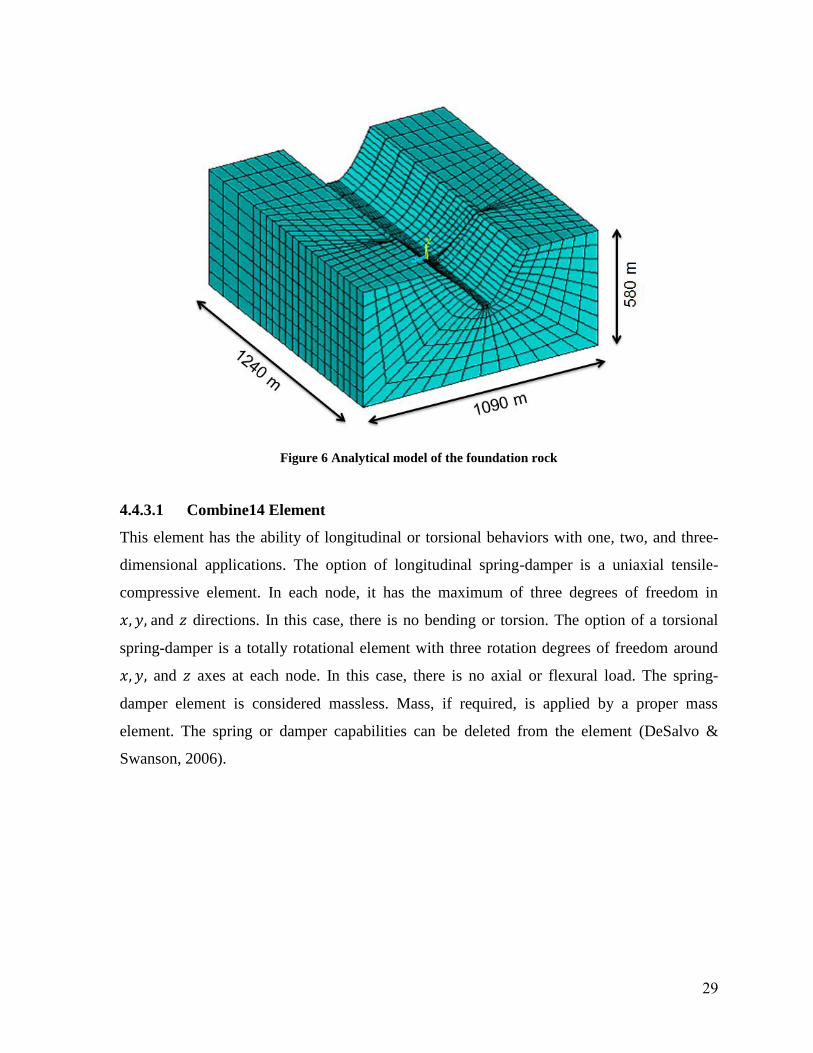
4.4.3 Finite Element Model of the Foundation

The interaction of dam-foundation interface has been considered while modeling the

foundation. In terms of the geometry, foundation resembles a rectangular cube that dam body

and hypothetical valley are removed from the upper surface of it. The model dimensions are

1240 𝑚 by 580 𝑚 by 1090 𝑚 corresponding to the length, height, and width, respectively. It

contains 3920 Solid45 elements (Figure 6).

To absorb the returning earthquake waves, which are caused by the movement of

seismic waves in the massed foundation, the viscous boundary condition is used. For this

purpose, a number of Combine14 spring-damper elements are used. They are connected to

the nodes around the foundation orthogonally in three directions. The vertical dampers

absorb the longitudinal waves. The dampers tangent on the surface absorb shear waves. The

bottom of the foundation is completely fixed.

29

Figure 6 Analytical model of the foundation rock

4.4.3.1 Combine14 Element

This element has the ability of longitudinal or torsional behaviors with one, two, and three-

dimensional applications. The option of longitudinal spring-damper is a uniaxial tensile-

compressive element. In each node, it has the maximum of three degrees of freedom in

𝑥, 𝑦, and 𝑧 directions. In this case, there is no bending or torsion. The option of a torsional

spring-damper is a totally rotational element with three rotation degrees of freedom around

𝑥, 𝑦, and 𝑧 axes at each node. In this case, there is no axial or flexural load. The spring-

damper element is considered massless. Mass, if required, is applied by a proper mass

element. The spring or damper capabilities can be deleted from the element (DeSalvo &

Swanson, 2006).

30

Chapter 5 Loadings, Analyses and Results

This chapter considers the loading characteristics, procedures and results of the different

types of analyses as well as the different factors affecting the behavior of arch dams. It has

been attempted that the considered assumptions match the real natural conditions as much as

possible.

5.1 Types of Loading

In this research, according to the preformed analysis, the combinations of the self-weight,

hydrostatic and hydrodynamic loads of the reservoir, seismic and thermal nodal loads are

applied. It should be mentioned that the critical static loading are combined of water pressure

at minimum reservoir level and thermal loading in summer critical time. It also includes

water pressure at maximum reservoir level and the thermal loading in winter critical time.

The results of the thermal loading are mentioned for these two states. In the usual and thin

arch dams, the uplift pressure has little effect and usually is not considered in the stress

analysis. The effect of hydrodynamic pressure of the reservoir in thin and light arch dams is

significant and critical. Because in such structures the added mass of the reservoir due to the

earthquake comparing to the self-weight is high. So, the response is extremely affected by the

dam-reservoir interaction. In thermal loading, the concrete temperatures in the different

nodes of the dam body are obtained from the thermal analyses. They are applied to the

analytical model as nodal loads. Seismic loading will be briefly described in continuation.

5.2 Seismic Loading

Considering site conditions, geotechnical properties, earth material, intensity and duration of

the earthquakes at different dam sites and comparing the records across the world with

similar geological conditions, the San Fernando earthquake of February 1971 was selected

(California Institute of Technology (Caltech), 2013). This earthquake has the magnitude of

6.6 on the Richter scale and happened at the approximate distance of 25 𝐾𝑚 from the fault

line and on the rigid soil. The maximum ground acceleration between the horizontal

components of the earthquake is 0.324𝑔, used along the river (x direction). The different

components of the earthquake acceleration record are displayed in Figure 7 to Figure 9.

31

5.2.1 Earthquake Frequency Content

Frequency content is the most important characteristic of an earthquake. If the dominant

frequency of the earthquake is equal to the frequency of the main vibration mode of the

structure, the resonance occurs. In this study, to determine the dominant frequency of the

earthquake, SeismoSignal software (Seismosoft Ltd., 2013), which processes the earthquake

information, is employed. This software calculates the dominant frequency of the earthquake

through Fourier Transform Amplitude method (Yilmaz, 2001). The results are displayed in

Figure 10. Since the main direction of impulse in the dam body is 𝑥, the dominant earthquake

frequency is determined according to the 𝑥 component of the acceleration record that is equal

to 2.93 𝐻𝑧.

5.2.2 Earthquake Duration

The amount of energy applied to the structure has direct relationship to the duration of the

earthquake. Higher earthquake duration means more energy on the structure. Analysis of the

structural systems such as arch dam-reservoir-foundation is time consuming. Due to

computational burden, rather than applying the whole earthquake time history record in the

analysis, the period and the related time history record in which the main energy of the

earthquake happens, are determined and applied on the structure. There are different methods

for the calculation of the earthquake duration such as Trifunac – Brady, Bolt – Beracket and

Maccann – Shah (Arias, 1970). This research employs SeismoSignal software which uses

Trifunac – Brady method (Seismosoft Ltd., 2013) to calculate earthquake duration. In this

method, the earthquake duration is when 5 to 95% of the total earthquake energy is applied

on the structure. Figure 11 illustrates an earthquake significant duration curve for the x

component of the earthquake. The significant duration for the earthquake is 15𝑠 in x direction

(from second 1 to 16), 13𝑠 in y direction (from second 1 to 14) and 15.5𝑠 in z direction (from

second 1 to 16.5). To be in the safe side, the first 18 seconds of the earthquake record is

applied in three directions.

32

Acc

eler

ati

on

(g)

Vel

oci

ty(m

/sec

)

Dis

pla

cem

en

t(m

)

Acc

eler

ati

on

Resp

on

se S

pec

tru

m(g

)

Figure 7 X-direction record of the earthquake

-0.2

-0.1

0

0.1

0.2

0.3

0 1 2 3 4 5 6 7 8 9 10 11 12 13 14 15 16 17 18 19 20 21 22 23 24 25 26 27 28 29 30

Time(sec)

Acce

lerat

ion(

g)

-0.15

-0.1

-0.05

0

0.05

0.1

0.15

0 1 2 3 4 5 6 7 8 9 10 11 12 13 14 15 16 17 18 19 20 21 22 23 24 25 26 27 28 29 30

Time(sec)

Velo

sity(

m/se

c)

-0.025

-0.02

-0.015

-0.01

-0.005

0

0.005

0.01

0.015

0 1 2 3 4 5 6 7 8 9 10 11 12 13 14 15 16 17 18 19 20 21 22 23 24 25 26 27 28 29 30

Time(sec)

Disp

lacem

ent(m

)

0

0.05

0.1

0.15

0.2

0.25

0.3

0.35

0.4

0.45

0.5

0.55

0.6

0.65

0.7

0.75

0.8

0.85

0.9

0.95

1

0 1 2 3 4

Period(sec)

Re

sp

on

se

Ac

ce

lera

tio

n(g

)

Damp 5%

33

Acc

eler

ati

on

(g)

Vel

oci

ty(m

/sec

)

Dis

pla

cem

en

t(m

)

Acc

eler

ati

on

Resp

on

se S

pec

tru

m(g

)

Figure 8 Y-direction record of the earthquake

-0.2

-0.15

-0.1

-0.05

0

0.05

0.1

0.15

0 1 2 3 4 5 6 7 8 9 10 11 12 13 14 15 16 17 18 19 20 21 22 23 24 25 26 27 28 29 30

Time(sec)

Acce

lera

tion(

g)

-0.08

-0.06

-0.04

-0.02

0

0.02

0.04

0.06

0.08

0 1 2 3 4 5 6 7 8 9 10 11 12 13 14 15 16 17 18 19 20 21 22 23 24 25 26 27 28 29 30

Time(sec)

Velo

city

(m/s

ec)

-0.015

-0.01

-0.005

0

0.005

0.01

0.015

0 1 2 3 4 5 6 7 8 9 10 11 12 13 14 15 16 17 18 19 20 21 22 23 24 25 26 27 28 29 30

Time(sec)

Disp

lace

men

t(m)

0

0.05

0.1

0.15

0.2

0.25

0.3

0.35

0.4

0.45

0.5

0.55

0.6

0.65

0.7

0 1 2 3 4

Period(sec)

Re

sp

on

se

Ac

ce

lera

tio

n(g

)

Damp 5%

34

Acc

eler

ati

on

(g)

Vel

oci

ty(m

/sec

)

Dis

pla

cem

en

t(m

)

Acc

eler

ati

on

Resp

on

se S

pec

tru

m(g

)

Figure 9 Z-direction record of the earthquake

-0.25

-0.2

-0.15

-0.1

-0.05

0

0.05

0.1

0.15

0.2

0.25

0.3

0 1 2 3 4 5 6 7 8 9 10 11 12 13 14 15 16 17 18 19 20 21 22 23 24 25 26 27 28 29 30

Time(sec)

Acce

lerat

ion(

g)

-0.15

-0.1

-0.05

0

0.05

0.1

0.15

0.2

0.25

0.3

0 1 2 3 4 5 6 7 8 9 10 11 12 13 14 15 16 17 18 19 20 21 22 23 24 25 26 27 28 29 30

Time(sec)

Velo

sity(

m/se

c)

-0.05

-0.04

-0.03

-0.02

-0.01

0

0.01

0.02

0 1 2 3 4 5 6 7 8 9 10 11 12 13 14 15 16 17 18 19 20 21 22 23 24 25 26 27 28 29 30

Time(sec)

Disp

lacem

ent(m

)

0

0.05

0.1

0.15

0.2

0.25

0.3

0.35

0.4

0.45

0.5

0.55

0.6

0.65

0.7

0 1 2 3 4

Period(sec)

Re

sp

on

se

Ac

ce

lera

tio

n(g

)

Damp 5%

35

Fo

uri

er A

mp

litu

de

Fo

uri

er A

mp

litu

de

Y component X component

Fo

uri

er A

mp

litu

de

Z component

Figure 10 Fourier Transform Amplitude of X, Y, and Z components of the earthquake

Ari

as

Inte

nsi

ty (

%)

Time (Sec)

Figure 11 Curve of the energy released during the earthquake for X component

0

0.01

0.02

0.03

0.04

0.05

0.06

0.07

0.08

0.09

0.1

0.11

0.0001 0.001 0.01 0.1 1 10 100

Frequency(Hz)

Fo

uri

er

Am

pli

tud

e

0

0.01

0.02

0.03

0.04

0.05

0.06

0.07

0.08

0.09

0.1

0.11

0.12

0.13

0.14

0.15

0.16

0.17

0.0001 0.001 0.01 0.1 1 10 100

Frequency(Hz)

Fo

uri

er

Am

pli

tud

e

0

0.01

0.02

0.03

0.04

0.05

0.06

0.07

0.08

0.09

0.1

0.11

0.12

0.13

0.14

0.15

0.16

0.17

0.18

0.19

0.2

0.0001 0.001 0.01 0.1 1 10 100

Frequency(Hz)

Fo

uri

er

Am

pli

tud

e

36

5.3 Thermal Analysis

The temperature distribution and its related thermal quantities in the whole system or in part

of it are calculated by thermal analysis. The usual thermal quantities contain temperature

distribution, lost or gained heat, thermal gradient and thermal flux. Generally, thermal

analysis aims to determine the thermal loading of the target system, to analyze and calculate

thermal stresses (DeSalvo & Swanson, 2006). The thermal input in the crown cantilever and

the results of thermal analyses of the upstream, downstream and central cantilever are

presented in Figure 12 and Figure 13, respectively. Temperature variations are visible

through the central cantilever profile. For winter time and NWL, approximate changes are

from 9 to 17 degrees on the foundation level and from 12 to 16 degrees on the crest level. For

summer time and MWL, temperature changes from 9 to 32 degrees on the foundation level

and from 28 to 32 degrees on the crest level.

Figure 12 Thermal input in the crown cantilever

37

DOWNSTREAM

UPSTREAM

WINTER (º C), NWL SUMMER (º C), MWL

Figure 13 Temperature distribution in the dam body for the summer and winter critical times

38

5.4 Stability Analysis

To check the stability and liability of the built model, static analysis is performed just on the

dam-massless foundation system without water. This analysis aims to consider the dam

stability under the dam weight before the application of operational loading. Figure 14

illustrates the distribution of the maximum principal stress (𝑆1) and minimum principal stress

(𝑆3) for downstream and upstream faces. Figure 15 displays the resulting displacement in 𝑥

direction.

DOWNSTREAM

UPSTREAM

S3 (N/m2) S1 (N/m2)

Figure 14 Distribution of the maximum principal stress (S1) and minimum principal stress (S3) for

downstream and upstream faces in the stability analysis

-.647E+07-.575E+07

-.503E+07-.431E+07

-.358E+07-.286E+07

-.214E+07-.141E+07

-69195730748

-.110E+07-598140

-94194409752

913698.142E+07

.192E+07.243E+07

.293E+07.343E+07

-.647E+07-.575E+07

-.503E+07-.431E+07

-.358E+07-.286E+07

-.214E+07-.141E+07

-69195730748

-.110E+07-598140

-94194409752

913698.142E+07

.192E+07.243E+07

.293E+07.343E+07

39

Figure 15 Distribution of the X direction displacement (m) in the stability analysis

According to the results, the maximum tension happens at the top corners of the upstream

and downstream. The maximum pressure happens around the dam heel. Comparing to the

allowable tensile and compressive strengths, the results are in acceptable range indicating no

failure for the dam.

5.5 Static Analysis

In this stage, the static analysis is done on the complete model of the dam-foundation-

reservoir under the dam and water self-weight, and the hydrostatic pressure. The results

obtained from the static analysis and thermal loading are utilized as the initial conditions for

the dynamic analysis. The distribution of 𝑆1 and 𝑆3 stresses for the upstream and

downstream faces in maximum water level condition is displayed in Figure 16. Furthermore,

the distribution of displacement in 𝑥 direction (upstream-downstream) in the dam body is

shown in Figure 17. The maximum tensile areas are around the dam heel. The maximum

compressive areas are along the walls and tow in the downstream, and in the middle and

upper parts of the upstream face. All stresses are in the safe zone except for a narrow strip in

the dam heel.

-.016504-.014561

-.012617-.010674

-.008731-.006788

-.004845-.002901

-.958E-03.985E-03

40

DOWNSTREAM

UPSTREAM

S3 (N/m2) S1 (N/m2)

Figure 16 Distribution of S1 and S3 for upstream and downstream faces in static analysis

Figure 17 Distribution of X direction displacement (m) in static analysis

-.863E+07

-.757E+07-.651E+07

-.544E+07-.438E+07

-.332E+07-.226E+07

-.119E+07-132002

930262 -.256E+07

-.142E+07-272490

871817.202E+07

.316E+07.430E+07

.545E+07.659E+07

.774E+07

-.863E+07

-.757E+07-.651E+07

-.544E+07-.438E+07

-.332E+07-.226E+07

-.119E+07-132002

930262 -.256E+07

-.142E+07-272490

871817.202E+07

.316E+07.430E+07

.545E+07.659E+07

.774E+07

0

.007295.01459

.021885.02918

.036475.04377

.051065.05836

.065655

41

5.6 Modal Analysis

The analysis of Rayleigh damping coefficients is a prerequisite for the dynamic analysis.

These coefficients themselves are dependent on the dominant vibration frequency of the

system. The natural frequencies and vibration mode shapes of the system can be determined

through modal analysis (Clough & Penzin, 1993). Due to the asymmetry of the mass system

of the fluid element, the determination of the vibration frequencies of the system in the

presence of water is very complicated. Therefore, modal analysis is performed without

reservoir elements. In dynamic analysis, because the dynamic modulus of elasticity applies to

the system, modal analysis is also carried out using dynamic modulus of elasticity. The

results of the performed analysis with the first fifteen natural frequencies are presented in the

Table 3. In addition, the shapes of the first seven vibration modes for the dam are presented

in Figure 18.

Table 3 Natural vibration frequencies for the first fifteen vibration modes of the system

Natural vibration frequency (Hrz) Vibration mode number

0.583035 1

0.616217 2

0.644124 3

0.736706 4

0.760074 5

0.809045 6

0.978767 7

0.998337 8

1.06159 9

1.07612 10

1.19599 11

1.21912 12

1.22859 13

1.28714 14

1.32452 15

42

mode 2 mode 1

mode 4 mode 3

mode 6 mode 5

mode 7

Figure 18 First seven vibration modes of the dam body

5.7 Dynamic Analysis

To consider the dynamic response of the structures under any kind of the time-varying loads,

the transient dynamic analysis is applied. In this procedure, the system equations of motion

are analyzed as a set of static equilibrium equations, considering inertial and damping forces

at any given time. The Newmark time integration method is used by the software to solve the

equations of motion (DeSalvo & Swanson, 2006). Generally, there are three full transient

dynamic analysis methods, namely direct method (Bathe & Wilson, Stability and accuracy

analysis of direct integration methods, 1973), reduced method (Huang & Huang, 2015), and

mode superposition method (Kuran & Özgüven, 1996). The method used in this study is

direct integration method, in which the matrices of mass, stiffness and damping of the whole

system is used in the analysis. However, the other methods do not include the whole system

43

in the analysis. Direct method is assumed stronger than the other methods for full transient

dynamic analysis, though the time spent in this method is more than others (DeSalvo &

Swanson, 2006).

5.7.1 Dynamic Analysis without Thermal Loading

In the beginning of each seismic analysis, a static analysis under the self-weight and

hydrostatic pressure is performed to determine the initial conditions of the system. Then, the

earthquake time-history record is applied to the model in three directions. Dynamic analyses

are carried out in the two states of normal and minimum water levels. To consider the results

of the dynamic analyses, 𝑆1 and 𝑆3 distribution envelopes for the upstream and downstream

faces, the time-history curve of the dam crest displacement in X direction, and the time-

history curve of 𝑆1 variations for 4 nodal points on the upstream and 4 nodal points on the

downstream are presented as shown in Figure 19. These points are selected as they have been

considered as part of the vulnerable areas to the maximum stresses.

Figure 19 Nodes used for consideration of dynamic analyses results on the dam upstream and

downstream faces

In brief, this part of the research performs linear dynamic analysis without thermal loading in

the two situations of a) with the reservoir NWL and b) with the reservoir MWL. The results

of these analyses are illustrated in Figure 20 to Figure 27.

44

Figure 20 S1 and S3 distribution envelops for the dam upstream and downstream faces in state (a)

S1(MPa)-MAX-DS

5.94187

5.55375

5.16562

4.7775

4.38937

4.00125

3.61312

3.225

2.83687

2.44875

2.06062

1.6725

1.28437

0.89625

0.508125

Frame 001 20 Apr 2009 DAM BODY CONTOURFrame 001 20 Apr 2009 DAM BODY CONTOUR

S1(MPa)-MAX-US

6.635

6.15

5.665

5.18

4.695

4.21

3.725

3.24

2.755

2.27

1.785

1.3

0.815

0.33

-0.155

Frame 001 20 Apr 2009 DAM BODY CONTOURFrame 001 20 Apr 2009 DAM BODY CONTOUR

S3(MPa)-MIN-DS

-2.5075

-3.055

-3.6025

-4.15

-4.6975

-5.245

-5.7925

-6.34

-6.8875

-7.435

-7.9825

-8.53

-9.0775

-9.625

-10.1725

Frame 001 20 Apr 2009 DAM BODY CONTOURFrame 001 20 Apr 2009 DAM BODY CONTOUR

S3(MPa)-MIN-US

-1.5925

-2.055

-2.5175

-2.98

-3.4425

-3.905

-4.3675

-4.83

-5.2925

-5.755

-6.2175

-6.68

-7.1425

-7.605

-8.0675

Frame 001 20 Apr 2009 DAM BODY CONTOURFrame 001 20 Apr 2009 DAM BODY CONTOUR

45

NO

DE

14

-UX

(m)

TIME(Sec)

Figure 21 Time-history curve for the dam crest displacement in X direction in state (a)

NO

DE

74

8-S

1(P

a)

NO

DE

75

0-S

1(P

a)

TIME(Sec) TIME(Sec)

NO

DE

78

7-S

1(P

a)

NO

DE

80

3-S

1(P

a)

TIME(Sec) TIME(Sec)

Figure 22 Time-history curves of S1 for the selected nodes in the dam upstream face in state (a)

-0.02

-0.01

0

0.01

0.02

0.03

0.04

0.05

0.06

0.07

0.08

0 2 4 6 8 10 12 14 16 18

Time(sec)

UX

(m)-

No

de

14

-1.00E+05

0.00E+00

1.00E+05

2.00E+05

3.00E+05

4.00E+05

5.00E+05

6.00E+05

7.00E+05

8.00E+05

0 3 6 9 12 15 18Time(sec)

S1(N

/m2)-

No

de748

-1.00E+05

0.00E+00

1.00E+05

2.00E+05

3.00E+05

4.00E+05

5.00E+05

6.00E+05

0 2 4 6 8 10 12 14 16 18Time(sec)

S1(N

/m2)-

No

de750

-4.00E+05

-2.00E+05

0.00E+00

2.00E+05

4.00E+05

6.00E+05

8.00E+05

1.00E+06

0 2 4 6 8 10 12 14 16 18Time(sec)

S1(N

/m2)-

No

de787

-2.00E+05

0.00E+00

2.00E+05

4.00E+05

6.00E+05

8.00E+05

1.00E+06

0 2 4 6 8 10 12 14 16 18Time(sec)

S1(N

/m2)-

No

de803

46

NO

DE

64

-S1

(Pa

)

TIME(Sec)

NO

DE

66

-S1

(Pa

)

TIME(Sec)

NO

DE

10

3-S

1(P

a)

TIME(Sec)

NO

DE

11

9-S

1(P

a)

TIME(Sec)

Figure 23 Time-history curves of S1 for the selected nodes in the dam downstream face in state (a)

-5.00E+05

0.00E+00

5.00E+05

1.00E+06

1.50E+06

2.00E+06

2.50E+06

3.00E+06

0 2 4 6 8 10 12 14 16 18

Time(sec) 20b

S1(N

/m2)-

No

de

64 2

4b

/22b

`

-5.00E+05

0.00E+00

5.00E+05

1.00E+06

1.50E+06

2.00E+06

2.50E+06

0 2 4 6 8 10 12 14 16 18

Time(sec)

S1(N

/m2)-

No

de

66

-1.00E+06

-5.00E+05

0.00E+00

5.00E+05

1.00E+06

1.50E+06

2.00E+06

2.50E+06

0 3 6 9 12 15 18

Time(sec)

S1(N

/m2)-

No

de

103

-1.00E+06

-5.00E+05

0.00E+00

5.00E+05

1.00E+06

1.50E+06

2.00E+06

2.50E+06

0 2 4 6 8 10 12 14 16 18Time(sec)

S1(N

/m2)-

No

de119

47

Figure 24 S1 and S3 distribution envelops for the dam upstream and downstream in state (b)

S1(MPa)-MAX-DS

5.13625

4.8125

4.48875

4.165

3.84125

3.5175

3.19375

2.87

2.54625

2.2225

1.89875

1.575

1.25125

0.9275

0.60375

Frame 001 22 Apr 2009 DAM BODY CONTOURFrame 001 22 Apr 2009 DAM BODY CONTOUR

S1(MPa)-MAX-US

6.635

6.15

5.665

5.18

4.695

4.21

3.725

3.24

2.755

2.27

1.785

1.3

0.815

0.33

-0.155

Frame 001 22 Apr 2009 DAM BODY CONTOURFrame 001 22 Apr 2009 DAM BODY CONTOUR

S3(MPa)-MIN-DS

-2.24375

-2.6775

-3.11125

-3.545

-3.97875

-4.4125

-4.84625

-5.28

-5.71375

-6.1475

-6.58125

-7.015

-7.44875

-7.8825

-8.31625

Frame 001 22 Apr 2009 DAM BODY CONTOURFrame 001 22 Apr 2009 DAM BODY CONTOUR

S3(MPa)-MIN-US

-2.03562

-2.40125

-2.76687

-3.1325

-3.49812

-3.86375

-4.22937

-4.595

-4.96062

-5.32625

-5.69187

-6.0575

-6.42312

-6.78875

-7.15437

Frame 001 22 Apr 2009 DAM BODY CONTOURFrame 001 22 Apr 2009 DAM BODY CONTOUR

48

NO

DE

14

-UX

(m)

TIME(Sec)

Figure 25 Time-history curve for the dam crest displacement in X direction in state (b)

NO

DE

74

8-S

1(P

a)

NO

DE

75

0-S

1(P

a)

TIME(Sec) TIME(Sec)

NO

DE

78

7-S

1(P

a)

NO

DE

80

3-S

1(P

a)

TIME(Sec) TIME(Sec)

Figure 26 Time-history curves of S1 for the selected nodes in the dam upstream face in state (b)

-0.02

-0.01

0

0.01

0.02

0.03

0.04

0.05

0.06

0.07

0.08

0 2 4 6 8 10 12 14 16 18

Time(sec)

UX

(m)-

No

de

14

-1.00E+05

4.00E+05

9.00E+05

1.40E+06

1.90E+06

2.40E+06

2.90E+06

0 3 6 9 12 15 18Time(sec)

S1

(N/m

2)-

No

de

74

8

-5.00E+05

0.00E+00

5.00E+05

1.00E+06

1.50E+06

2.00E+06

2.50E+06

3.00E+06

3.50E+06

4.00E+06

0 2 4 6 8 10 12 14 16 18Time(sec)

S1(N

/m2)-

No

de750

-4.00E+05

-2.00E+05

0.00E+00

2.00E+05

4.00E+05

6.00E+05

8.00E+05

1.00E+06

1.20E+06

0 2 4 6 8 10 12 14 16 18Time(sec)

S1(N

/m2)-

No

de787

-2.00E+05

0.00E+00

2.00E+05

4.00E+05

6.00E+05

8.00E+05

1.00E+06

1.20E+06

1.40E+06

1.60E+06

0 2 4 6 8 10 12 14 16 18Time(sec)

S1(N

/m2)-

No

de803

49

NO

DE

64

-S1

(Pa

)

TIME(Sec)

NO

DE

66

-S1

(Pa

)

TIME(Sec)

NO

DE

10

3-S

1(P

a)

TIME(Sec)

NO

DE

11

9-S

1(P

a)

TIME(Sec)

Figure 27 Time-history curves of S1 for the selected nodes in the dam downstream face in state (b)

-1.00E+06

0.00E+00

1.00E+06

2.00E+06

3.00E+06

4.00E+06

5.00E+06

0 2 4 6 8 10 12 14 16 18

Time(sec) 20b

S1(N

/m2)-

No

de

64 2

4b

/22b

`

-5.00E+05

0.00E+00

5.00E+05

1.00E+06

1.50E+06

2.00E+06

2.50E+06

3.00E+06

0 2 4 6 8 10 12 14 16 18

Time(sec)

S1(N

/m2)-

No

de

66

-1.00E+06

-5.00E+05

0.00E+00

5.00E+05

1.00E+06

1.50E+06

2.00E+06

2.50E+06

3.00E+06

3.50E+06

0 3 6 9 12 15 18

Time(sec)

S1(N

/m2)-

No

de

103

-5.00E+05

0.00E+00

5.00E+05

1.00E+06

1.50E+06

2.00E+06

2.50E+06

3.00E+06

3.50E+06

4.00E+06

0 2 4 6 8 10 12 14 16 18Time(sec)

S1(N

/m2)-

No

de119

50

According to the results of state (a), the maximum tensile areas are the dam top corners and

around the heel and tow, in the upstream and downstream faces, and also in the upper part of

the downstream near the crest. The maximum compressive areas are along the walls, near the

tow, and around the top middle of the downstream, and also along the middle of the crest in

the upstream. Comparing to the allowable tensile and compressive strengths, all areas are in

the acceptable range, unless for the upstream top left and right corners where tensile failure

happens. The same dynamic analysis was conducted for state (b). The maximum tensile areas

are top corners of the dam in the upstream and downstream especially in the upstream right

corner, in the middle of the crest in the downstream and especially in the upstream, and

around the heel and tow. The maximum compressive areas are along the walls, tow, and

around the top middle of the downstream, and along the middle of the crest in upstream.

Comparing to the allowable tensile and compressive strengths, all areas are in the safe zone,

unless for the upstream top right corner where tensile failure can happen.

5.7.2 Dynamic Analysis with Thermal Loading

In this stage, in addition to the previously mentioned loadings, the nodal temperatures are

also applied on the dam body in the initial static analysis. Then, in the presence of initial

thermal and static stresses, the linear dynamic analysis is performed in two states of c) in the

winter critical time with the reservoir NWL and d) in the summer critical time with the

reservoir MWL. The related results are represented in the Figure 28 to Figure 35.

51

Figure 28 S1 and S3 distribution envelops for the dam upstream and downstream faces in state (c)

S1(MPa)-MAX-DS

6.27188

5.83375

5.39563

4.9575

4.51938

4.08125

3.64313

3.205

2.76688

2.32875

1.89063

1.4525

1.01437

0.57625

0.138125

Frame 001 04 May 2009 DAM BODY CONTOURFrame 001 04 May 2009 DAM BODY CONTOUR

S1(MPa)-MAX-US

8.14188

7.56375

6.98563

6.4075

5.82938

5.25125

4.67313

4.095

3.51688

2.93875

2.36063

1.7825

1.20438

0.62625

0.048125

Frame 001 04 May 2009 DAM BODY CONTOURFrame 001 04 May 2009 DAM BODY CONTOUR

S3(MPa)-MIN-DS

-2.08375

-2.6475

-3.21125

-3.775

-4.33875

-4.9025

-5.46625

-6.03

-6.59375

-7.1575

-7.72125

-8.285

-8.84875

-9.4125

-9.97625

Frame 001 04 May 2009 DAM BODY CONTOURFrame 001 04 May 2009 DAM BODY CONTOUR

S3(MPa)-MIN-US

-0.815625

-1.20125

-1.58687

-1.9725

-2.35812

-2.74375

-3.12937

-3.515

-3.90062

-4.28625

-4.67187

-5.0575

-5.44312

-5.82875

-6.21437

Frame 001 04 May 2009 DAM BODY CONTOURFrame 001 04 May 2009 DAM BODY CONTOUR

52

NO

DE

14

-UX

(m)

TIME(Sec)

Figure 29 Time-history curve for the dam crest displacement in X direction in state (c)

NO

DE

74

8-S

1(P

a)

NO

DE

75

0-S

1(P

a)

TIME(Sec) TIME(Sec)

NO

DE

78

7-S

1(P

a)

NO

DE

80

3-S

1(P

a)

TIME(Sec) TIME(Sec)

Figure 30 Time-history curves of S1 for the selected nodes in the dam upstream face in state (c)

-0.01

0

0.01

0.02

0.03

0.04

0.05

0.06

0.07

0.08

0 2 4 6 8 10 12 14 16 18

Time(sec)

UX

(m)-

No

de

14

-1.00E+05

1.00E+05

3.00E+05

5.00E+05

7.00E+05

9.00E+05

0 3 6 9 12 15 18Time(sec)

S1

(N/m

2)-

No

de

74

8

-1.00E+05

0.00E+00

1.00E+05

2.00E+05

3.00E+05

4.00E+05

5.00E+05

6.00E+05

7.00E+05

8.00E+05

0 2 4 6 8 10 12 14 16 18Time(sec)

S1(N

/m2)-

No

de750

1.00E+05

3.00E+05

5.00E+05

7.00E+05

9.00E+05

1.10E+06

1.30E+06

1.50E+06

1.70E+06

0 2 4 6 8 10 12 14 16 18Time(sec)

S1

(N/m

2)-

No

de

78

7

0.00E+00

3.00E+05

6.00E+05

9.00E+05

1.20E+06

1.50E+06

1.80E+06

0 2 4 6 8 10 12 14 16 18Time(sec)

S1(N

/m2)-

No

de803

53

NO

DE

64

-S1

(Pa

)

TIME(Sec)

NO

DE

66

-S1

(Pa

)

TIME(Sec)

NO

DE

10

3-S

1(P

a)

TIME(Sec)

NO

DE

11

9-S

1(P

a)

TIME(Sec)

Figure 31 Time-history curves of S1 for the selected nodes in the dam upstream face in state (c)

-5.00E+05

0.00E+00

5.00E+05

1.00E+06

1.50E+06

2.00E+06

2.50E+06

3.00E+06

0 2 4 6 8 10 12 14 16 18

Time(sec) 20b

S1(N

/m2)-

No

de

64 2

4b

/22b

`

-5.00E+05

0.00E+00

5.00E+05

1.00E+06

1.50E+06

2.00E+06

2.50E+06

0 2 4 6 8 10 12 14 16 18

Time(sec)

S1(N

/m2)-

No

de

66

-1.00E+06

-5.00E+05

0.00E+00

5.00E+05

1.00E+06

1.50E+06

2.00E+06

0 3 6 9 12 15 18

Time(sec)

S1(N

/m2)-

No

de

103

-1.00E+06

-5.00E+05

0.00E+00

5.00E+05

1.00E+06

1.50E+06

0 2 4 6 8 10 12 14 16 18Time(sec)

S1

(N/m

2)-

No

de1

19

54

Figure 32 S1 and S3 distribution envelops for the dam upstream and downstream faces in state (d)

S1(MPa)-MAX-DS

4.6825

4.285

3.8875

3.49

3.0925

2.695

2.2975

1.9

1.5025

1.105

0.7075

0.31

-0.0875

-0.485

-0.8825

Frame 001 05 May 2009 DAM BODY CONTOURFrame 001 05 May 2009 DAM BODY CONTOUR

S1(MPa)-MAX-US

6.8975

6.435

5.9725

5.51

5.0475

4.585

4.1225

3.66

3.1975

2.735

2.2725

1.81

1.3475

0.885

0.4225

Frame 001 05 May 2009 DAM BODY CONTOURFrame 001 05 May 2009 DAM BODY CONTOUR

S3(MPa)-MIN-DS

-3.11437

-3.61875

-4.12312

-4.6275

-5.13188

-5.63625

-6.14063

-6.645

-7.14938

-7.65375

-8.15813

-8.6625

-9.16688

-9.67125

-10.1756

Frame 001 05 May 2009 DAM BODY CONTOURFrame 001 05 May 2009 DAM BODY CONTOUR

S3(MPa)-MIN-US

-0.815625

-1.20125

-1.58687

-1.9725

-2.35812

-2.74375

-3.12937

-3.515

-3.90062

-4.28625

-4.67187

-5.0575

-5.44312

-5.82875

-6.21437

Frame 001 05 May 2009 DAM BODY CONTOURFrame 001 05 May 2009 DAM BODY CONTOUR

55

NO

DE

14

-UX

(m)

TIME(Sec)

Figure 33 Time-history curve for the dam crest displacement in X direction in state (d)

NO

DE

74

8-S

1(P

a)

NO

DE

75

0-S

1(P

a)

TIME(Sec) TIME(Sec)

NO

DE

78

7-S

1(P

a)

NO

DE

80

3-S

1(P

a)

TIME(Sec) TIME(Sec)

Figure 34 Time-history curves of S1 for the selected nodes in the dam upstream face in state (d)

-0.08

-0.06

-0.04

-0.02

0

0.02

0.04

0 2 4 6 8 10 12 14 16 18

Time(sec)

UX

(m)-

No

de

14

-5.00E+05

0.00E+00

5.00E+05

1.00E+06

1.50E+06

2.00E+06

2.50E+06

3.00E+06

3.50E+06

4.00E+06

0 3 6 9 12 15 18Time(sec)

S1

(N/m

2)-

No

de

74

8

-5.00E+05

5.00E+05

1.50E+06

2.50E+06

3.50E+06

4.50E+06

5.50E+06

0 2 4 6 8 10 12 14 16 18Time(sec)

S1(N

/m2)-

No

de750

1.00E+05

3.00E+05

5.00E+05

7.00E+05

9.00E+05

1.10E+06

1.30E+06

1.50E+06

1.70E+06

0 2 4 6 8 10 12 14 16 18Time(sec)

S1

(N/m

2)-

No

de

78

7

0.00E+00

3.00E+05

6.00E+05

9.00E+05

1.20E+06

1.50E+06

1.80E+06

2.10E+06

0 2 4 6 8 10 12 14 16 18Time(sec)

S1(N

/m2)-

No

de803

56

NO

DE

64

-S1

(Pa

)

TIME(Sec)

NO

DE

66

-S1

(Pa

)

TIME(Sec)

NO

DE

10

3-S

1(P

a)

TIME(Sec)

NO

DE

11

9-S

1(P

a)

TIME(Sec)

Figure 35 Time-history curves of S1 for the selected nodes in the dam upstream face in state (d)

0.00E+00

5.00E+05

1.00E+06

1.50E+06

2.00E+06

2.50E+06

3.00E+06

3.50E+06

4.00E+06

4.50E+06

0 2 4 6 8 10 12 14 16 18

Time(sec) 20b

S1(N

/m2)-

No

de

64 2

4b

/22b

`

0.00E+00

2.00E+05

4.00E+05

6.00E+05

8.00E+05

1.00E+06

1.20E+06

1.40E+06

1.60E+06

1.80E+06

2.00E+06

0 2 4 6 8 10 12 14 16 18

Time(sec)

S1(N

/m2)-

No

de

66

-1.50E+06

-5.00E+05

5.00E+05

1.50E+06

2.50E+06

3.50E+06

4.50E+06

0 3 6 9 12 15 18

Time(sec)

S1(N

/m2)-

No

de

103

-1.50E+06

-5.00E+05

5.00E+05

1.50E+06

2.50E+06

3.50E+06

4.50E+06

0 2 4 6 8 10 12 14 16 18Time(sec)

S1(N

/m2)-

No

de119

57

According to the results of state (c), the maximum tensile areas are the dam top corners and

around the heel and tow, in the upstream and downstream faces, and also in the upper part of

the downstream near the crest. The maximum compressive areas are along the walls, near the

tow, and around the top middle of the downstream, and also along the middle of the crest in

the upstream. Comparing to the allowable tensile and compressive strengths, all areas are in

the acceptable range, except for the upstream top left and right corners where more intense

tensile failure happens. The same dynamic analysis was done for state (d). The maximum

tensile areas are near top corners of the dam in the upstream and downstream especially in

the upstream right corner, in the middle of the crest in the downstream and especially in the

upstream, and around the tow and mostly the heel. The maximum compressive areas are

around the tow and middle of the downstream face and along the middle of the crest and at

the top corners in the upstream. Comparing to the allowable tensile and compressive

strengths, all areas are in the safe zone, except for the upstream top right corner and middle

of the crest, where more intense tensile failure can happen. By adding thermal effects, the

max tensile and compressive areas are nearly the same, but the stress distribution, levels, and

failure points are somehow different.

58

Chapter 6 Conclusion

6.1 Conclusions

The comparison of the results of the dynamic analyses with and without thermal loading, i.e.

comparing the state (a) with the state (c) as well as comparing the state (b) with the state (d)

indicates that:

In the dynamic analysis with thermal loading in the winter critical time and NWL (state

c):

1. The overall values for the maximum tensile S1 (the upper limit of S1 contour) in the

upstream and downstream of the dam are more than the maximum tensile S1 in the

dynamic analysis without thermal loading (state a).

2. The values for the minimum tensile S1 (the lower limit of S1 contour) are generally

more in the upstream and less in the downstream, compared with the minimum tensile

S1 in the dynamic analysis without thermal loading (state a).

3. The values for the maximum compressive S3 and minimum compressive S3 are

generally less than the similar parameters in the dynamic analysis without thermal

loading (state a).

In the dynamic analysis with thermal loading in the summer critical time and MWL (state

d):

1. The values for the maximum tensile S1 (the upper limit of S1 contour) are generally

more in the upstream and less in the downstream compared with the maximum tensile

S1 in the dynamic analysis without thermal loading (state b).

2. The values for the minimum tensile S1 (the lower limit of S1 contour) are generally

more in the upstream and less in the downstream, compared with the minimum tensile

S1 in the dynamic analysis without thermal loading (state b).

3. The values for the maximum compressive S3 are generally less in the upstream and

downstream and the values for the minimum compressive S3 are more in the

downstream and less in the upstream compared to the similar parameters in the

dynamic analyses without thermal loading (state b).

Overall, in the dynamic analysis with thermal loading, in winter critical time and NWL

(state c), S1 values for the downstream face, except for the right and left corners of the

59

crest, are less and for the upstream face, except for the heel, are more than the similar

values in cases without thermal loading (state a).

In the dynamic analysis with thermal loading in the summer critical time and MWL (state

d), S1 values for the downstream face, except for the upper right and left corners and the

toe, is less, and for the upstream face, is more than the cases without thermal loading

(state b).

In the stress distribution envelop for the dam upstream and downstream faces in the

dynamic analysis with thermal loading at winter critical time and NWL (state c), S3

values, except for the toe and side of the abutments of downstream, are mostly less than

the corresponding values in the dynamic analysis without thermal loading (state a).

In the dynamic analysis with thermal loading at summer critical time and MWL (state d),

S3 values are mostly more for the downstream face, except for the upper left and right

corners and slightly higher than the toe than the corresponding values in the dynamic

analysis without thermal loading (state b). S3 values are mostly less for the upstream face,

except for the middle and upper left corner, than the state (b). The above results indicate

that, in overall, the application of thermal loading increases the tension values in 50% of

cases and decrease the compression values in 75% of cases in the dam body.

The maximum displacement of the dam crest in x direction (Ux) toward the downstream

in the central cantilever and downstream face due to the thermal loading at winter critical

time and NWL (state c) is higher than Ux produced at similar times in the situations

without thermal loading. Also, Ux due to the thermal loading at summer critical time and

MWL (state d) is less than Ux produced at similar times in the situations without thermal

loading. Therefore, it can be concluded that, due to the thermal loading, the difference

between the maximum and minimum displacement remains constant in each diagram

comparing to the cases without thermal loading. But, the dam crest in the central

cantilever moves toward upstream in 75% of cases during thermal loading. S1 values for

the selected nodes at winter critical time and NWL (state c) in upstream and downstream

faces are respectively more and less than the S1 values in the analysis without thermal

loading.

Finally, this research revealed that the application of thermal loading in the dynamic

analysis of an arch dam is necessary. Thermal effects changed the results of dynamic

60

analyses. They increased the maximum tension, changed the maximum pressure, and

decreased the displacements. Since the effects of various states of heat distribution on the

values of compressive and tensile stresses in the dam body are different, the critical

thermal states should be applied on the dam and their effects should be examined

separately. The comparison of the time history of the displacement of the dam crest in the

above states indicates that the displacement of the dam crest while applying thermal

loading is less than its displacement while there is no thermal loading.

6.2 Recommendations

The following suggestions are recommended for more realistic studies in the future:

Study the reservoir-foundation interaction effects on the static and dynamic response

of the arch dams more precisely.

Investigate the effects of damping on the seismic response of arch dams by

performing parametric studies.

Evaluate more detailed boundary conditions and to compare the effectiveness of

different types of boundary conditions on the seismic response of arch dams with

massed foundation.

Research the effect of long-term thermal loading on the concrete strength and the

concrete dam response.

Assess short-term changes (daily and hourly) in ambient temperature and the concrete

hydration heat into thermal analyses.

Analyze the effect of thermal gradients on the dynamic response of the dam body

considering the impact of contraction and horizontal joints and non-linear behavior of

the concrete in the dam body.

61

References

Agullo, L., & Aguado, A. (1995). Thermal behavior of concrete dams due to environmental

actions. Dam Engineering, 6, 3-21.

Agullo, L., Mirambell, E., & Aguado, A. (1996). A model for the analysis of concrete dams

due to environmental thermal effects. International Journal of Numerical Methods for

Heat & Fluid Flow, 6(4), 25-36.

Arias, A. (1970). A Measure of Earthquake Intensity (Seismic Design for Nuclear Power

Plants ed.). (R. J. Hansen, Ed.) Cambridge, Massachusetts: MIT Press.

Bathe, K. J., & Wilson, E. L. (1967). Numerical methods in finite element analysis.

Englewood Cliffs, New Jersey: PRENTICE-HALL, INC.

Bathe, K. J., & Wilson, E. L. (1973). Stability and accuracy analysis of direct integration

methods. Earthquake Engineering and Structural Dynamics, 1(3), 283-291.

Bofang, Z. (1997). Prediction of Water Temperature in Deep Reservoir. Dam Engineering,

8(1), 13-25.

California Institute of Technology (Caltech). (2013, January 31). Significant Earthquakes

and Faults. Retrieved 3 2013, from Southern California Earthquake Data Center:

http://scedc.caltech.edu/significant/sanfernando1971.html

Canadian Electricity Association. (1990). Safety assessment of existing dams for earthquake

conditions. Vol. C-4, Seismic Analysis of Concrete Dams, CEA Rep. No. 420 G 547.

Montreal: Canadian Electricity Association.

Chopra, A. K. (1967, December). Hydrodynamic Pressure on Dames during Earthquakes.

Journal of the Engineering Mechanics Division, 93(EM6), 205-223.

Clough, R., & Penzin, J. (1993). Dynamics of Structures (Vol. 2). McGraw-Hill Inc.

Daoud, M., Galanis, N., & Ballivy, G. (1997). Calculation of the periodic temperature field

in a concrete dam. Canadian Journal of Civil Engineering, 24(5), 772-784.

DeSalvo, G. J., & Swanson, J. A. (2006). ANSYS user's manual. Houston, PA: Swanson

Analysis Systems.

Federal Energy Regulatory Commission. (1999). Engineering guidelines for the evaluation of

hydropower projects. Chapter 11-Arch Dams. Division of Dam Safety and

Inspections. Washington DC, 20426: Federal Energy Regulatory Commission.

62

Fok, K.-L., Hall, J. F., & Chopra, A. K. (1996). EACD-3D: A Computer Program for Three-

dimensional Earthquake Analysis of Concrete Dams. Report No. UCB/ EERC-86/09.

Berkeley: University of California.

Ghaemian, M., & Ghobarah, A. (1998). Staggered Solution Schemes for Dam-Reservoir

Interaction. Journal of Fluids and Structures(12), 933-948.

Ghaemian, M., & Ghobarah, A. (1999). Nonlinear Seismic Analysis of Concrete Gravity

Dams Including Dam-Reservoir Interaction. Engineering Structures, 21, 306-315.

Hariri-Ardebili, M. A., & Kianoush, M. R. (2014). Integrative seismic safety evaluation of a

high concrete arch dam. Soil Dynamics and Earthquake Engineering, 67, 85-101.

Huang, Y. H., & Huang, Y. (2015). Adaptive Reduced Basis Methods Applied to Structural

Dynamic Analysis. American Journal of Computational Mathematics, 5, 317-328.

Humar, J., & Roufaiel, M. (1983, February). Finite Element Analysis of Reservoir Vibration.

Journal of Engineering Mechanics, 109(1), 215-230.

ICOLD. (1984). Détérioration des barrages et réservoirs, recueuil de cas et analyse.

Brookfield, VT: A.A. Balkema Publishers.

Iran Water & Power Resources Development Co. (2004). Karun IV dam and power plant

project, the final stage studies. No. 1200-29.

Javanmardi, F., Léger, P., & Tinawi, R. (2005). Seismic water pressure in cracked concrete

gravity dams. Journal of Structural Engineering, 131(1).

Knight, D. J., & Mason, P. J. (1992). Lessons from the effect of earthquakes on dams. Water

Power and Dam Constr, 44(3), 44–46.

Kuran, B., & Özgüven, H. N. (1996). A modal superposition method for non-linear

structures. Journal of Sound and vibration, 189(3), 315-339.

Leger, P., Venturelli, J., & Bhattacharjee, S. S. (1993). Seasonal Temperature and Stress

Distribution in Concrete Gravity Dams.Part 1 & 2: Behaviour. Canadian Journal of

Civil Engineering, 20(6), 999-1029.

Li, Q., Liang, G., Hu, Y., & Zuo, Z. (2014). Numerical analysis on temperature rise of a

concrete arch dam after sealing based on measured data. Mathematical Problems in

Engineering, 2014.

List25 LLC. (2014, December 19). 25 Tallest Dams in the World. Retrieved December 2015,

from List 25: http://list25.com/25-tallest-dams-in-the-world/2/

63

Liu, X., Zhang, C., Chang, X., Zhou, W., & Cheng, Y. (2015). Precise simulation analysis of

the thermal field in mass concrete with a pipe water cooling system. Applied Thermal

Engineering, 78, 449-459.

Lysmer, J., & Kuhlemeyer, R. L. (1969). Finite Dynamic Model for Infinite Media. Journal

of the Engineering Mechanics Division, 95(4), 859-877.

Meyer, T., & Mouvet, L. (1995). Behaviour Analysis of the Vieux-Emosson Arch Gravity

Dam under Thermal Loads. Dams Engineering, 6(LCH-ARTICLE-1995-001), 275-

292.

Mirzabozorg, H., & Varmazyari, M. (2009). Concrete Gravity Dams and Traveling Wave

Effect along Reservoir Bottom. International Journal of Civil, Environmental,

Structural, Construction and Architectural Engineering and Technology, 3(10).

Mirzabozorg, H., Hariri-Ardebili, M. A., Shirkhan, M., & Seyed-Colbadi, S. M. (2014).

Mathematical modeling and numerical analysis of thermal distribution in arch dams

considering solar radiation effect. The Scientific World Journal, 2014.

Raphael, J. M. (1984, March-April). Tensile Strength of Concrete. ACI Journal, Technical

Paper(Title No. 81-17).

Regan, P. J. (2010, 06 01). Dams & Civil Structures: An Examination of Dam Failures vs.

Age of Dams. Retrieved 06 2015, from HydroWorld.com:

http://www.hydroworld.com/articles/hr/print/volume-29/issue-4/articles/dams--civil-

structures.html

Rixen, D., Farhat, C., & Géradin, M. (1998). A two-step, two-field hybrid method for the

static and dynamic analysis of substructure problems with conforming and non-

conforming interfaces. Computer methods in applied mechanics and engineering,

154(3), 229-264.

Seismosoft Ltd. (2013, 07 19). SeismoSignal v5.1. Retrieved 08 2013, from SEiSMOSOFT

EARTHQUAKE ENGINEERING SOFTWARE SOLUTIONS:

http://www.seismosoft.com/SeismoSignal-v5.1.2

Serafim, I. L., & Oliveira, C. S. (1987). Effects caused by earthquakes on dams. ICOLD

Symposium (p. Beijing). international committee on large dams.

64

Sharan, S. K. (1985). Finite Element Analysis of Unbounded and Incompressible Fluid

Domains. International Journal for Numerical Methods in Engineering, 21, 1659-

1669.

Sharan, S. K. (1987). Time-Domain Analysis of Infinite Fluid Vibration. International

Journal for Numerical Methods in Engineering, 24, 945-958.

Sheibany, F., & Ghaemian, M. (2006). Effects of Environmental Action on Thermal Stress

Analysis of Karaj Concrete Arch Dam. Journal of Engineering Mechanics, 132(5),

532–544.

Stucky, A., & Derron, M. H. (1957). Thermal Problems Related to Construction of Dam-

Reservoir. Lausanne: P. Feissly, Ed., E`cole Polytechnique, De L`universite De

Lausanne, Publication No. 38.

Tatalovich, J. (1998). Comparison of Failure Modes from Risk Assessment and Historical

Data for Bureau of Reclamation Dams. DSO-98-01. Bureau of Reclamation, Dam

Safety Office. U.S. Department of Interior.

Tehrani, M. R., Ghaemian, M., & Rofooei, F. R. (2005). Evaluation of the Seismic response

of concrete arch dams including the foundation mass. Water and Energy Abstracts, 15

(4).

Tinawi, R., Léger, P., Leclerc, M., & Cipolla, G. (2000). Seismic safety of gravity dams:

from shake table experiments to numerical analyses. Journal of Structural

Engineering, 126(4), 518-529.

U. S. Army Corps of Engineers. (1994). Arch dam design: Engineering and design. Engineer

Manual 110-2-2201. Washington, D.C.: Dept. of the Army, Corps of Engineers,

Office of the Cheif Engineers.

U. S. Army Corps of Engineers. (2003). Time-History Dynamic Analysis of Concrete

Hydraulic Structures; Chapter 2 and 3. EM 1110-2-6051. Washington, D.C.: Dept. of

the Army, Corps of Engineers, Office of the Chief of Engineers.

U.S. Army Corps of Engineers. (1995). Engineering and design, gravity dams. Rep. EM

1110- 2-2200. Washington, D.C.: U.S. Army Corps of Engineers.

Wang, H. B., Qiang, S., Sun, X., & Zheng, R. (2011, October). Dynamic simulation analysis

of temperature field and thermal stress of concrete gravity dam during construction

period. In Applied Mechanics and Materials, 90, 2677-2681.

65

White, F. M., & Corfield, I. (2006). Viscous fluid flow (Vol. 3). New York: McGraw-Hill.

Wolf, J. P. (1988). Soil-Structure-Interaction Analysis in Time Domain. New Jersey: Prentice

Hall Englewood Cliffs.

Wolf, J. P., & Song, C. (1995). Doubly Asymptotic Multi-Directional Transmitting Boundary

for Dynamic Unbounded Medium-Structure-Interaction Analysis. Earthquake

Engineering and Structural Dynamics, 24, 175-188.

Wolf, J. P., & Song, C. (1996). Finite-Element Modeling of Unbounded Media. John Wily

and Sons.

Yilmaz, Ö. (2001). Seismic Data Analysis: Processing, Inversion, and Interpretation of

Seismic Data (Vol. 1). (S. M. Doherty, Ed.) Tulsa, OK: Society of Exploration

Geophysicists.

Zhang, Z., & Garga, V. K. (1996). State of temperature and thermal stress in mass concrete

structures subjected to thermal shock. Dam Engineering, 7, 336-350.

Zhou, J., Lin, G., Zhu, T., Jefferson, A. D., & Williams, F. W. (2000). Experimental

investigations into seismic failure of high arch dams. Journal of Structural

Engineering, 126(8), 926-935.

66

Appendix A: Permission Request

Dear Ryhane Moghadas Jafari:

Permission is granted for you to reuse figure 2 from "Effects of Environmental Action on Thermal Stress Analysis of Karaj Concrete Arch Dam" for your Thesis.

A full credit line must be added to the material being reprinted. For reuse in non-ASCE publications, add the words "With permission from ASCE" to your source citation. For Intranet posting, add the following additional notice: "This material may be downloaded for personal use only. Any other use requires prior permission of the American Society of Civil Engineers.”

Regards,

Joann

Joann Fogleson Manager, Product and Subscription Services American Society of Civil Engineers 1801 Alexander Bell Drive Reston, VA 20191

PERMISSIONS@asce.org

703-295-6112

E-mail: jfogleson@asce.org Internet: www.asce.org/pubs | www.ascelibrary.org | http://ascelibrary.org/page/rightsreque

sts

A full credit line must be added to the material being reprinted. For reuse in non-ASCE publications, add the words "With permission from ASCE" to your source citation. For Intranet posting, add the following additional notice: "This material may be downloaded for personal use only. Any other use requires prior permission of the American Society of Civil Engineers.”

Each license is unique, covering only the terms and conditions specified in it. Even if you have obtained a license for certain

ASCE copyrighted content, you will need to obtain another license if you plan to reuse that content outside the terms of the existing license. For example: If you already have a license to reuse a figure in a journal, you still need a new license to use the same figure in a magazine. You need separate license for each edition