dynamic attending and responses to time - accueilpift6080/h09/documents/papers/boltzjones.pdf ·...
TRANSCRIPT

Psycholosical Review Copyright 1989 by the American Ps~holo#cal Association, Inc. 1989, Vol. 96, No. 3, 459--491 0033-295X/89/$00.75
Dynamic Attending and Responses to Time
Mari Riess Jones Marilyn Boltz Ohio State University Haverford College
A temporally based theory of attending is proposed that assumes that the structure of world events affords different attending modes. Future-oriented attending supports anticipatory behaviors and occurs with highly coherent temporal events. Time judgments, given this attending mode, axe influ- enced by the way an event's ending confirms or violates temporal expectancies. Analytic attending supports other activities (e.g., grouping, counting), and if it occurs with events of low temporal coherence, then time judgments depend on the attending levels involved. A weighted contrast model describes over- and underestimations of event durations. The model applies to comparative duration judgments of equal and unequal time intervals; its rationale extends to temporal productions/extrap- olations. Two experiments compare predictions of the contrast model with those derived from other traditional approaches.
One characteristic of modern society is a preoccupation with fixed time schedules and standardized timekeepers. We main- tain appointments at hourly intervals, rush to meet the 5:00 p.m. bus, and dine at predetermined hours. Yet our natural ability to judge time remains poorly understood. How often do we estimate the time elapsed since last glancing at a clock and discover with surprise that we were fairly accurate? Surprise is understandable because at least as often we lose track of time and err. The validity of these impressions is confirmed by labo- ratory research showing that duration judgments depend not only on actual physical duration but also on a variety of non- temporal factors. These include the spatial layout and complex- ity of an event as well as the attentional set, skill, affect, and constitutional state of the judge (Allan, 1979; Fraisse, 1984; Kristofferson, 1984).
Researchers have addressed many of these issues that include both psychophysical problems (e.g., Weber's Law for time dis- crimination) and organismic variables (e.g., age, drugs, and arousal effects). Of recent interest is the influence of nontempo- ral information on time judgments, due largely to a fascination with such problems as the filled interval effect. This phenome- non reveals that two equivalent time intervals may not be judged as such because of the nontemporal information that fills them. Although the most popular models of judged dura- tion attempt to explain this effect (e.g., Block, 1978; Ornstein, 1969), the effect itself raises problems for a general theory of time estimation (Allan, 1979).
In this article we focus on some problems raised by the filled
This research was supported by Grant BNS-8204811 from the Na- tional Science Foundation and by a fellowship from the Netherlands Institute for Advanced Study awarded to the senior author (I 986-1987).
The authors thank Chris Antons, David Buffer, Walter Johnson, Gary Kidd, Kerri Marsh, Elizabeth Maxshburn, John Michon, Mitch Pratt, Ken Pugh, Jackie Ralston, and Wither wan Vreden. Special thanks axe due to Steve Handel and two anonymous reviewers for their excellent comments on an earlier version of this article.
Correspondence concerning this article should be addressed to Marl Riess Jones, Department of Psychology, The Ohio State University, 142 Townshend Hall, Columbus, Ohio 432 I0.
459
interval effect. We consider these and related issues concerning responses to time from a more general perspective, one based on an analysis of event time itself and dynamic aspects of at- tending. We suggest that events define time intervals and that their inherent rhythmic patternings will affect the way people attend to them and judge their durations. The general frame- work leads to hypotheses about duration judgments of both equal and unequal time intervals as well as temporal extrapola- tions. Although these hypotheses cannot explain all of the di- verse facts of time estimation, they do suggest ways of linking a general theory of attending to specific models of time judgment and discrimination. In this, our approach is not intended to usurp contemporary time models but to incorporate some of their assumptions into a more inclusive framework.
This article has five parts. Part 1 introduces some contempo- rary time models. Part 2 outlines a theoretical approach to event time and dynamic attending, and Part 3 returns to time estimation and poses specific hypotheses about dynamic at- tending in various tasks. Part 4 describes two experiments rele- vant to these hypotheses that present difficulties for contempo- rary time models. Part 5 concludes with additional theoretical implications of this approach.
Par t 1: C o n t e m p o r a r y Theories and Issues
In Part 1, several contemporary models of judged duration are presented along with relevant empirical support. These models primarily address the case in which people judge identi- cal durations and errors give rise to the filled interval effect. One influential model is Ornstein's (1969).
Ornstein's Storage Size Hypothesis
Influenced by Frankenhauser's (1959) original model, Ornstein (1969) further developed the storage size hypothesis to explain the estimation of time periods lasting about 10 s or more. According to this view, two equal time intervals will seem to have different durations if one is more complex and therefore requires more storage space in memory: "The central metaphor is that the experience of duration of an interval is a construction

460 MARI RIESS JONES AND MARILYN BOLTZ
formed from its storage size. As storage size increases, duration experience lengthens" (Ornstein, 1969, p. 42).
Experiments supporting this view have relied on various definitions of stimulus complexity (e.g., number of angles in visual figures, stimulus arrangement in time and space) and found that the experienced duration of intervals between 30 s and I0 min does, in fact, lengthen with increasing stimulus complexity (Hogan, 1975; Ornstein, 1969; Schiffman & Bobko, 1974). Others, however, have reported conflicting results. For example, both Block (1974) and Poynter (1983) have found that a sequence of words is judged longer when words are grouped by semantic category than when randomly arranged. Because the latter presumably contains more chunks, this contradicts Ornstein's model. As a result of these discrepancies, models as- suming a different referent for judged duration have been pro- posed.
Attentional Effort Models
A model offered by Underwood and Swain (1973) posits that duration judgments are mediated by attentional effort. They tested Ornstein's (1969) prediction that increased attention leads to more stored information and hence to longer time esti- mates. Attentional demands were varied independently of in- formation content in a vigilance task in which subjects detected target digits embedded in prose passages that were partially masked by various white noise intensities. When unexpectedly asked to judge the relative duration of each passage, subjects reported those masked by a high-intensity noise (i.e., requiring more attention) to be longer than those masked by a low-inten- sity noise. However, contrary to Ornstein's storage analysis, de- tection levels indicated that less information was encoded in highly masked passages.
Such findings support the idea that experienced duration is less dependent on memory load than on attentional effort or arousal associated with presented information. Others, using very brief stimuli, have reached similar conclusions (Thomas & Cantor, 1978; Thomas & Weaver, 1975).
Contextual Change Model
Another challenge to Ornstein's (1969) proposal comes from Block's (1978, 1985, in press) contextual change hypothesis. Judged duration is hypothesized to increase as a linear function of the number of contextual changes occurring in both the envi- ronmental situation (e.g., changes in stimulus properties, task demands) and in the organism (e.g., mnemonic activities). Changes are monitored by an internal cognitive device that later outputs a complexity index based on the total number of changes within a time interval.
In one test of this model, Block and Reed (1978) required subjects to encode word lists at different levels of processing (h la Craik & Lockhart, 1972). For example, some people judged the typing style of words (i.e., a shallow task) or categorized words into semantic categories (i.e., a deep task), whereas others alternated between both tasks. Afterward, all of the subjects were unexpectedly asked to judge which activity seemed longer. Both the storage size and attentional effort models predict that deep processing (more information, more effort) should pro- duce longer time estimates. This was not the case. When people
alternated shallow--deep strategies (i.e., more changes), dura- tion seemed longer. They interpreted such findings as support for Block's change hypothesis and as pgoblematic for both the storage size and attentional effort models.
Evaluation of Current Models
How successful are these models? Each is quite successful within certain contexts. However, all share certain empirical and theoretical limitations.
Empirical difficulties stem from seemingly conflicting results that emerge from the literature as a whole. An interval defined as more complex is sometimes judged longer, but on other occa- sions is judged shorter than a less complex one. For example, divergent results have been observed with the variables of stimu- lus familiarity (e.g., Avant & Lyman, 1975, vs. Devane, 1974), task difficulty (e.g., Burnside, 1971, vs. Underwood & Swain, 1973), and stimulus arrangement (e.g., Poynter, 1983, vs. Schiffman & Bobko, 1974).
Some conflicting findings may be due to methodological differences. Others, however, suggest a need for re-evaluating certain tacit assumptions of the models themselves (also see Block, in press). In particular, three issues are relevant.
The first involves the presumed referent for duration judg- ments. Each model assumes that time judgments are inferred from the amount of some processing activity. Howev~, this pro- cessing activity strictly refers to the nontemporal information that fills the stimulus interval: the number of spatial angles, the arrangement of word lists, the amount of background noise, and so on. But the temporal information within an event and its impact on behavior is ignored.
A second problem concerns complexity. Complexity is as- sumed to increase the amount of processing activity and thereby lengthen experienced duration. But it isn't always clear why. The relationship of psychological complexity to the stimu- lus or its duration is rarely fully developed. For example, the storage size hypothesis claims that complexity is determined by the number of memory chunks. Although recent coding theo- ries add formalization by equating complexity with memory code length (e.g., Deutsch & Feroe, 1981; Leeuwenberg, 1969; Simon, 1972), it remains a difficult construct. What exactly is a chunk, and what stimulus or task characteristics determine chunk boundaries? Such questions have never been satisfacto- rily answered. Complexity determinants of attentional effort and cognitive change are equally elusive. In a speech utterance, for example, there are changes in sound, grammar, meaning, and intonation, and yet we don't know which kind or how much . of a change is required to affect judged duration. Because con- temporary time models lack precise definitions of complexity, this may partially explain the conflicting nature of experimental results.
A final problem concerns the choice of experimental stimuli. During the course of a day, we interact with friends, drive, listen to music, and so on. Yet, these kinds of events are rarely selected for study. Instead, subjects must compare intervals filled with smile abstract drawings (Ornstein, 1969), clicks (Adams, 1977), and lists of unrelated words or nonsense words (Poynter, 1983). Although the latter may offer tight experimental control and may in fact represent certain everyday experiences, they fail to reflect the full range of stimuli we routinely experience.

DYNAMIC ATTENDING 461
Commonplace events differ from those typical of traditional time studies in several ways, notably in their structure and func- tion. With respect to structure, events such as speech utter- ances, musical patterns, and body movements contain much more structural coherence in time than those of current re- search. Typically, these events display multiple levels of interre- lated structure that unfold predictably over a given time span. Often there is distinctiveness as natural time patterns, including special beginnings and endings, characteristic tempi, and rhythms. All of this contributes to temporal predictability. And predictability allows perceivers to anticipate an event's future course, including when in time it should end. In interactive speech, for example, the smooth exchange of speaking roles and turn-taking behavior suggests that people anticipate ends of ut- terances. In other cases, event structure can communicate mood or intention. It is possible that the structure and function of events systematically affect time estimation.
In sum, contemporary research on time estimation is charac- terized by conflicting experimental findings. At the same time, questions can be raised about the structure, function, and rep- resentativeness of stimuli used in this research. We suggest that these are related problems. Divergent experimental findings arise because variations in the structure of temporal events and the ways people respond to them have not been considered.
Overview of an Alternative Hypothesis of Judged Duration
An alternative perspective takes its cue from the idea that events are, by definition, temporal and that their structure in
t ime is critical. That is, the temporal patterning of nontemporal information (e.g., words, tonal pitches, lights, and even haphaz- ard items) within any interval is critical in determining how one attends to the event itself. Societal and individual needs ensure that all kinds of events are encountered, but we claim that peo- ple attend differently to events with high and low structural co- herence, and that this, in turn, differentially affects time esti- mates. In brief, we propose a distinction between two different modes of dynamic attending, future-oriented and analytic, that can bias time estimates of events with high and low coherence, respectively.
Events I differ in terms of their structural coherence and pre- dictability. And although we assume a continuum of coherence, for convenience we distinguish between events with high and low temporal coherence. Highly coherent events, such as those of speech, tonal music, and body gestures, offer structural pre- dictability and display characteristic rhythmic patterns that oc- cur over nonarbitrary time spans. Events of low coherence, such as a list of unrelated words or simultaneous cocktail-party chat- ter, unfold over arbitrary time spans that contain little struc- tural predictability.
Highly coherent events afford future-oriented attending. Be- cause they offer high temporal predictability, people can track and use higher order time patternings to generate expectancies about how and when they will end. In Western music, for exam- ple, notes within an unfolding melody occur in a temporally ordered fashion, often with such coherence that listeners can anticipate not only what notes are likely but also when in time they "should" occur. Thus, future-oriented attending exploits the global time structure of such events. In these situations, we
propose that time estimates are determined by the confirmation or violation of expected ending times. When two events of equivalent duration both end when expected, people will cor- rectly judge them to be the same duration. However, if one vio- lates an expectancy by seeming to end later than anticipated, then it will be incorrectly judged as longer. Similarly, an event appearing to end too early will be judged as relatively short. This reasoning extends to judgments of events that actually do differ in duration. According to this view then, duration esti- mates of coherent events are biased by temporal contrast where contrast involves an apparent temporal disparity between an event's actual and expected ending.
Analytic attending occurs with less coherent events. These events have low temporal predictability, and so people cannot anticipate their future course. Instead, they are forced to attend locally to adjacent elements in an attempt to organize the un- structured information. Depending on the task, this kind of at- tending supports strategies directed toward lower level relation- ships (e.g., grouping or counting the number of items or changes within the event). Finally, to estimate the duration of these events, people will be biased by their attention to local details and will judge events filled with more items to be longer.
Both future-oriented and analytic attending are dynamic ways of interacting with temporal events. In this article the em- phasis will be on future-oriented attending and its influence on time estimates, inasmuch as this topic has received less atten- tion than the memory-oriented approach found in contempo- rary time models.
Summary of Part I
Contemporary time models have focused on the filled inter- val effect in which nontemporal information distorts judgments about equal time intervals. Their explanations rely on memory- based processes that gauge the total amount of a nontemporal construct (i.e., complexity, effort, change). But these ap- proaches encounter problems of divergent empirical support, imprecise definitions of complexity, and lack of stimulus repre- sentativeness. An alternative view is presented that is more ex- plicitly temporal. It proposes two modes of dynamic attending (future-oriented, analytic) that occur with events of high and low temporal coherence, respectively. This model is designed to accommodate diverse experimental findings by supplementing memory-oriented attending (analytic) with future-oriented at- tending.
Par t 2: Tempora l Env i ronmen t and At tunement s
In the remainder of this article, we have three goals. The first is to show that analyses of event structure are critical to theories
Cognitive approaches have traditionally referred to world objects and experimental materials as stimuli. In protest to implications regard- ing the impoverished nature of such materials, some recent approaches have adopted the term event to refer to ecologically valid objects under- going physical motion or change (Gibson, 1966, 1979). Our framework reflects both notions in that an event refers to any environmental object or activity that varies along a continuum of structural coherence. Some natural events are very predictable in that embedded temporal relation- ships are lawfully interrelated with the event's nontemporal informa- tion. Other natural events are less coherent and predictable in this re- gard and, in fact, may contain little internal structure (e.g., silences).

462 MARl RIESS JONES AND MARILYN BOLTZ
of attending. The second is to describe distinct ways in which people can attend to events that vary in temporal coherence. The third is to demonstrate that both event structure and at- tending mode must be considered when building theories of time estimation.
Part 2 addresses the first goal. Any interpretation of re- sponses to time should be based on a theory about what time means in events and to people who perceive these events. In this approach, time means relative time. Our formalization leads to dynamic conceptions of event structure, temporal predictabil- ity, and complexity. It also leads to hypotheses about the ease with which people can use dynamic structure to attend in vari- ous ways, some of which operate in time estimations.
Theoretical Background
A relativistic approach to time implies that points in time and absolute time intervals are less important than time periods determined relative to other time periods (rhythmic structure) and time periods determined relative to spatial extents (velocity or flow structure; Jones, 1976). These time relations are insepa- rable from the event itself. This idea is at the heart of our asser- tion that people may be unreliable when judging absolute lengths of arbitrary or isolated time intervals.
Our theoretical emphasis on relative time is consistent with an ecological analysis of event structure in terms of transforma- tions (changes) and invariants (nonchanges) and their functions for the organism (Freyd, 1987; Gibson, 1979; Jones, 1976; Shaw, McIntyre, & Mace, 1974; Shepard, 1984; Turvey & Ca- rello, 1981). People and other living things both create and re- spond to temporal event structure found in conversations, dance, music, and so on. We suggest further that time transfor- mations often support these interactions in special ways. This leads to a different approach to complexity and, ultimately, to the way people respond to dynamic event structure. To preview, in subsequent sections we propose that events characterized by certain time transformations are easier to anticipate in time (Jones, 1976, 1981 a, 1982; D. N. Lee, 1980; Michon & Jackson, 1985).
Relative Time in Environmental Structure
Our environment is filled with all sorts of temporal events, some based on activities of living things and others not. All lie on a continuum of temporal coherence ranging from highly ar- bitrary (low coherence) to nonarbitrary (high coherence). The gist of temporal coherence was presented in Part 1 where it was related to temporal predictability and attending mode. Here, we introduce greater formalization by distinguishing between temporally coherent, or hierarchical (H) time structures, and temporally incoherent, or nonhierarchical (NH) ones. Ulti- mately, complexity is dynamically conceived in terms of these time structures.
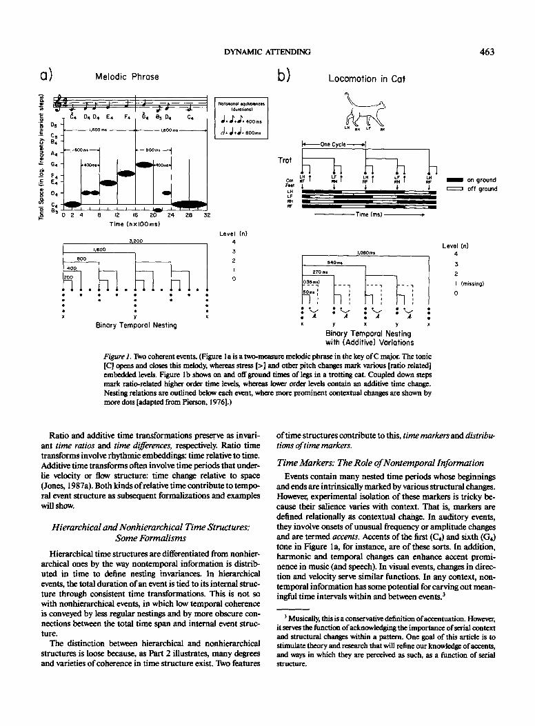
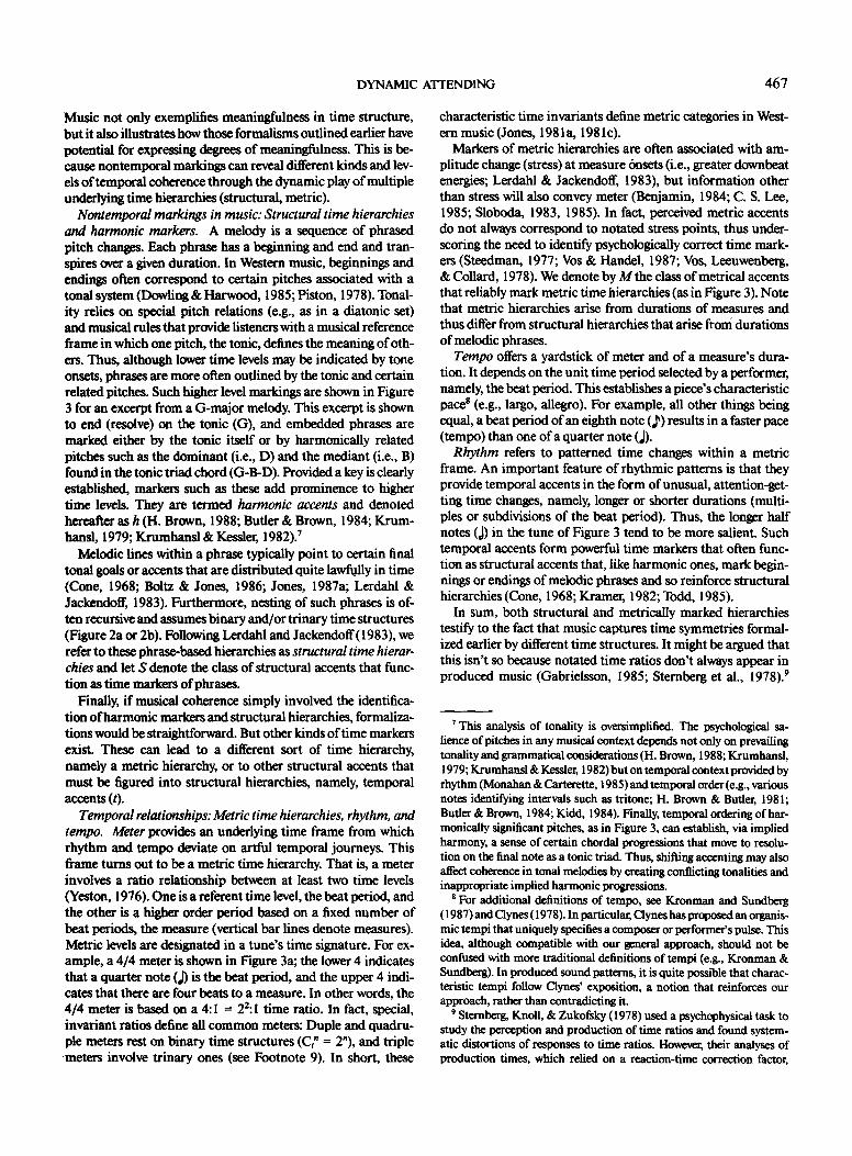
We begin with some examples of temporally coherent (hier- archical) events in Figure la and lb. Both examples illustrate our use of the term coherent to imply objective accent regulari- ties (i.e., not necessarily subjective experiences). In each, non- temporal information is distributed in ways that convey much predictability in time. In Figure la, a musical phrase of 3,200 ms is prominently outlined by salient opening and closing
pitches (C4). 2 Lawfully embedded within this span are other time periods (e.g., 1,600, 800 ms), also significantly identified by onsets of various pitches. The smallest time period (200 ms) is determined by the smallest observable tone-to-tone onset in- terval. Another hierarchical event is illustrated in Figure lb, in which cycles of a cat's locomotion sequence are shown to em- bed on-ground time periods (e.g., 270 ms) and smaller periods. Notice that the former are more strongly marked by co-occur- fing downsteps of two legs (from left hind [LH] with right front [RF] ~, to left front [LF] with right hind [RH] ~). Below each event is an abstraction of its nesting properties showing relevant sets of time periods (n = 0, 1, 2 . . . ). Onsets of more prominent time levels are usually marked by more salient nontemporal information (more dots at, e.g., locations x and y).
These examples highlight two points. One involves identifi- cation of distinctive nontemporal markings of varions time lev- els. The other involves clarification of lawfulness in temporal nestings. The issue of distinctive markings is an experimental problem to which we return in later sections. The issue of law- fulness concerns time rules that we formalize as time transfor- mations.
A time transformation changes one time period into others while preserving some temporal property as invariant (Jones, 1976, 1981c). Thus, i f a 200-ms time period is nested within one of 400 ms, and this, in turn, is nested in an 800-ms period, as in Figure I a, then one of the simplest time transformations results in which all time levels are related in a binary fashion via multiples of 2 (i.e., period doubling). This sort of change is a ratio time transformation. It is one of two types of transforma- tions that enter into temporal coherence. The other is an addi- tive time transformation. If200 ms is changed into 250 ms and then 300 ms, an invariant additive change of +50 ms exists. Often, additive time changes enter into temporal nestings as variations within a given level. For example, in Figure lb the level n = 0 (50 ms) reflects a recurrent change o f - 8 5 ms with respect to the (missing) periodicity of level n = I (135 ms; dashed line). In contrast to ratio time transformations, which operate vertically to change level n into n + I (or vice versa), additive transformations operate horizontally to modulate peri- odicities recurring at some fixed level.
2 A musical scale is defined by a set of pitch classes and relationships among these pitches. Of most relevance to Western classical music are diatonic scales, composed of seven pitch classes. Diatonic scales are formed by a series of pitch changes (musical intervals) involving whole steps (w) and half-steps (s), where w = 2s, and s (also called semitone) is a unit difference. The half-step, or semitone unit, is logarithmically defined as a frequency ratio: A fff = .05946. A major diatonic scale, beginning on the keynote or tonic, has the following sequence of whole steps and half-steps: w, w, s, w, w, w, s. Thus, the most familiar major diatonic scale is C major, in which suoeessive pitch classes of CDEF- GABC are separated by w, w, s, w, w, w, s. In this scale, successive pitch classes are referred to as scale degrees with C being the first scale degree, D the second, E the third, and so on (see Hahn & Jones, 1981). Some important harmonic relationships within each scale include a major third (e.g., C-E in C-major scale), which corresponds to the pitch changes of(w, w) from an initial referent pitch, and a perfect fifth (e.g., C-G), which corresponds to the scale steps of(w, w, s, w). The mediant (E) is the note that defines a major third, whereas the dominant is the note (G) that defines a perfect fifth above the tonic (C). Together the notes C-E-G form the tonic triad chord in C major.
DYNAMIC ATTENDING 463
O) Melodic Phrase
~4 D4 D4 E4 F4 ~4 B3 D4 C4 g o~ os c - - C s
g ~. A,,
G,,
g' F,,
_ C4 o 8 3
- - 1,600 ms ~ 160Oral
0 2 4 8 12 16 20 24 28 32
T i m e (n x l O 0 ms)
1,600
eoo
.hl.
Binary Temporal Nesting
Nolo,lanai equi~lences (durations)
J, ,1+,1. eoo.
b) Locomotion in Cat
mt LF RF
< One Cycle ) [
Cat RF RF RH RF Fee, ~ ~, ,I. ~. ; LH I LF 1 I " Rid m I RF I
Time (ms) ~,
Leve l (n)
4
3
2
I
O
I,OeOm$
S4Oms
x y x y
Binary Temporal Nesting with (Additive) Variations
Figure 1. Two coherent events. (Figure I a is a two-measure melodic phrase in the key of C major. The tonic [C] opens and closes this melody, whereas stress [>] and other pitch changes mark various [ratio related] embedded levels. Figure Ib shows on and off ground times of legs in a trotting cat. Coupled down steps mark ratio-related higher order time levels, whereas lower order levels contain an additive time change. Nesting relations are outlined below each event, where more prominent contextual changes are shown by more dots [adapted from Pierson, 1976].)
1 on ground , o f f ground
Level (n) 4 5 2 I (missing) 0
Ratio and additive time transformations preserve as invari- ant time ratios and time differences, respectively. Ratio time transforms involve rhythmic embeddings: time relative to time. Additive time transforms often involve time periods that under- lie velocity or flow structure: time change relative to space (Jones, 1987a). Both kinds of relative time contribute to tempo- ral event structure as subsequent formalizations and examples will show.
Hierarchical and Nonhierarchical Time Structures: Some Formalisms
Hierarchical time structures are differentiated from nonhier- archical ones by the way nontemporal information is distrib- uted in time to define nesting invariances. In hierarchical events, the total duration of an event is tied to its internal struc- ture through consistent time transformations. This is not so with nonhierarchical events, in which low temporal coherence is conveyed by less regular nestings and by more obscure con- nections between the total time span and internal event struc- ture.
The distinction between hierarchical and nonhierarchical structures is loose because, as Part 2 illustrates, many degrees and varieties of coherence in time structure exist. Two features
of time structures contribute to this, time markers and distribu- tions of time markers.
Time Markers: The Role of Nontemporal Information
Events contain many nested time periods whose beginnings and ends are intrinsically marked by various structural changes. Howeve~ experimental isolation of these markers is tricky be- cause their salience varies with context. That is, markers are defined relationally as contextual change. In auditory events, they involve onsets of unusual frequency or amplitude changes and are termed accents. Accents of the first (C4) and sixth (G4) tone in Figure la, for instance, are of these sorts. In addition, harmonic and temporal changes can enhance accent promi- nence in music (and speech). In visual events, changes in direc- tion and velocity serve similar functions. In any context, non- temporal information has some potential for carving out mean- ingful time intervals within and between events. 3
; Musically, this is a conservative definition of accentuation. However, it se~ves the function of acknowledging the importance of serial context and structural changes within a pattern. One goal of this article is to stimulate theory and research that will refine our knowledge of accents, and ways in which they are perceived as such, as a function of serial structure.
Hierarchical (rhythmic) Time Structures Level (n)
ATI~
3 A T ~
I
O • • • •
• . : • : • : • :
B i n a r y T i m e S t r u c t u r e
b ) : ...... " h 1 o ° . . . . . . . . . h . l . .
T r i n a r y T i m e S t ruc tu re
4
c), ~Tz
~T~
~-~, ,~, V o V o V o V
B i n a r y T i m e S t r u c t u r e wi th V a r i a t i o n s
~T n
C, = ~T,~.I = 2
A T n Ct = ~Tn_ I = 3
A T n Ct= '=2
ATn-I
fo r n > I
d) Non-Hierarchical Time Structures
~ T 3
o o • o o • o e • e l • o o • e l •
Binary with T r i n a r y T i m e S t ruc tu res (Polyrhythm)
e) ~ 4
,c,T~
) / ~__, . k • . : • :
.~.h.h.. N o n - hierarchical
Top Ct = 2-
Bottom
ATn = 8 / 6 = % Ct = ATn. I
O= Accent Type I • = Accent Type 2
First Half Ct =2
Second Half C t=5 ,4
f )
Non-h ierarch ica l
O = Unaccented ( l ight of f )
• = Accented ( l ight on)
DYNAMIC ATTENDING 465
Accents differ in relative strength (or prominence). In Figure 1 (lower portions) more dots indicate greater accent strength that is associated with greater energy change and/or multiple accent occurrences. Thus, the simultaneous occurrence of am- plitude change (i.e., the > stress notation) with certain special pitch changes (C~ or (34) in Figure 1 a, or that of an LH downstep with an R F one in Figure lb, renders these stronger markings. Coupled accents are in fact typically stronger than decoupled ones. Furthermore, stronger accents tend to mark higher time levels in coherent time hierarchies (Benjamin, 1984; Jones, 1976, 1987a; Lerdahl & Jackendoff, 1983; Martin, 1972). In what follows, we assume that it is possible to reliably determine functional markers at different t ime levels.
Distributions o f T ime Markers: Role o f T ime Transformations
The term hierarchy has been variously used (Jones, 1981b). Here it refers to a time structure in which the temporal distribu- tion of markers reveals nested time levels that are consistently related to one another at a given level by ratio or additive time transformations. Conversely, to the degree that a distribution of time markers does not reveal this consistency in time transfor- mations, a nonhierarchical time structure of greater dynamic complexity occurs.
In hierarchical events, each nested level is associated with a recurrent time period, denoted by AT,, in which AT refers to the marked time span and n refers to a level in the hierarchy (n = 0, 1, 2 . . . . ). The smallest t ime period, denoted ATo, oc- curs at the lowest level and is often marked, especially initially, by onsets of certain adjacent elements. In an ideal hierarchy, other nested periods are related to AT0 by sets of simple time ratios (or ratio time transformations). 4 Thus, the total duration of a hierarchical event is implied by the time period of any em- bedded level.
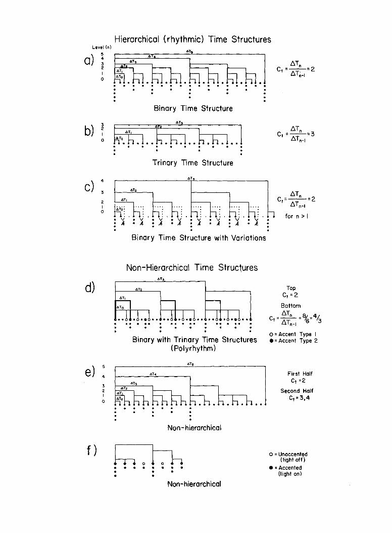
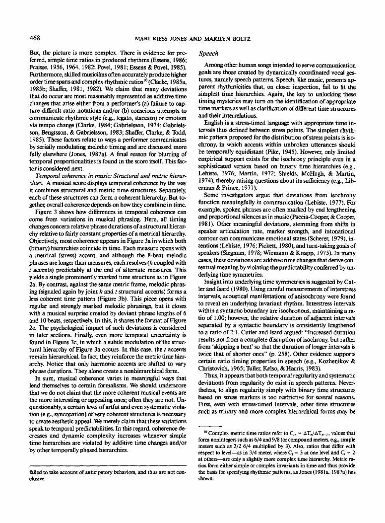
Figure 2 presents three examples of hypothetical time hierar- chies that range in temporal coherence from very high to mod- erate. The first, and simplest, is shown in Figure 2a. It is merely an extension of the binary structure shown in Figure la. All nested time levels are related by a ratio time transform of 2. Thus, the smallest level, ATo, is related to AT~ by 2, to AT2 by 4, and so on, until its total duration is linked to all others. This is a binary time structure. It is hierarchical because the nesting is consistent, meaning that the same ratio (here 2) obtains over recurrent periods at each level. Such a ratio is a time rule and will be denoted as Ct,, in which Ct, = ATJATn - 1 (for levels n, n - 1). This time rule operates vertically to summarize tem- poral nesting. Finally, in this binary structure, Ctn is an invari- ant in that it is constant over different levels, n: C,, = Cz = 2.
Simple time hierarchies are based on Ct values that are small and constant integers (i.e., Ct = 1, 2, 3, etc.). When Ct = 3, a
trinary structure results as in Figure 2b. This hierarchy is less coherent than the binary one because the time ratio involves a larger integer. When different C, values appear at different levels (e.g., C,m --'- 2, and Ctn = 3; n = 1 . . . m . . . p . . . ) more complex hierarchies are specified. 5
Finally, a moderately complex hierarchy is shown in Figure 2c. This is a binary hierarchy with additive time changes (shown as k). This change essentially shifts the (missing) ATI to form the lowest time level, much as in the cat example of Figure lb. In other cases, if such shifts consistently apply to stronger ac- cents (higher level), interesting syncopated versions of this hier- archical form may be specified. All such structures are hierar- chical for two reasons: (a) The additive transform is invariant for all periods at a given level, and (b) other time levels (here n > 1) are consistently related by Ct = 2.
All of these time structures exhibit consistent temporal nest- ing. In those with simple time symmetries (e.g., Ct = 1, 2, 3 . . . ) , this takes on a tight recursive form that draws on ratio time invariance. Any higher time period (AT,) can be related to the unit period by a power of the constant ratio, C,:
ATn = AToCt n (where n = 0, 1, 2, . . . ) . (1)
Temporal recursiveness is important. This expression indicates how it ties an event together dynamically by showing that any embedded time level can be consistently transformed into any other via time ratios.
In sum, hierarchical time structures display regular, ratio- based temporal nestings within an event's total duration, as well as consistent additive modulations to this ratio base. In terms of dynamic complexity, hierarchies fall into two general catego- ries: those that do not incorporate additive time rules (Figure 2a and 2b) and those that do (Figure 2c). Degree of temporal coherence can be loosely gauged by the value and constancy of underlying ratio time rules, with more coherent events falling into the first category. Conversely, dynamic complexity is greater for hierarchies of the second category in which variable, larger, or noninteger ratio time transforms might occur. This
4 One may argue that ATn reflects translatory time transformations forming an infinite symmetry group, and that Ct n (n = 0, + 1 + 2 +- 3) reflects dilatory time transformations that also form an infinite symme- try group (e.g., Hahn & Jones, 1981; Coxeter & Greitzer, 1967). For a more general treatment in terms of time transformations that specify the logarithmic spiral, see Hahn and Jones.
5 This analysis assumes an established time structure and functional markers. If the time structure refers to meters, for example, it is not concerned with issues of meter identification and ways in which certain markers, beat periods, and rhythmic figures may facilitate meter identi- fication on the part of an attender (Essens & Povel, 1985; Longnet-Hig- gins & Lee, 1982, 1984). These issues involve attending and detection of temporal invariants and are considered in a later section.
Figure 2. Six examples of time structures that could hypothetically characterize a given environmental event. (Examples range from the binary time structure of (a) that is highly coherent (hierarchical) to the irregular one of low coherence in (f) that is nonhierarchical. The latter represents a temporal pattern of lights, in on [O] or off [O] positions, from a judged duration study by Poynter and Homa [ 1983]. In all patterns the stronger accents are signified by more dots. Temporal level, AT,, corresponds to the recurrent period at n = 0, 1 . . . . . Nesting properties are given by ratio time transformations, Ct, = ATn/ATn-~.)
466 MARI RIESS JONES AND MARILYN BOLTZ
reasoning extends to assessments of nonhierarchieal time struc- tures, three of which appear in Figure 2 (i.e., 2d, 2e, 2f).
Figure 2d illustrates an important kind of nonhierarchieal time structure. It is a polyrhythm. A polyrhYthm involves two simultaneously recurrent periodicities that form a noninteger time ratio (e.g., 4:3 and 4:5; Apel, 1972). It is literally a tempo- ral phasing of two time hierarchies. In this case, binary and trinary time structures are involved, each identified by a different accent type (O or O) that becomes coupled (O) only to mark higher levels. Thus, Figure 2d has a hierarchical counter- part in Figure 2c: Both display a higher level binary time struc- ture. But the polyrhythm lacks the consistent additive time changes of Figure 2c at its lower levels (in which time ratios are 4:3 or 8:6; Handel, 1984; Handel & Oshinsky, 1981; Yeston, 1976).
A different sort of violation of hierarchical time symmetry occurs in Figure 2e. Here, prominent accents reveal a temporal nesting that is initially hierarchical. However, this regularity of 8 beats is clearly violated in the second half of the sequence, in which higher order time spans of 10 and 6 beats occur. A more complex time ratio is thus needed to formalize this structure.
Finally, the most irregular time pattern (Figure 20 embeds durations that are haphazardly marked at higher levels, yielding low temporal coherence. This time structure is one we hypothe- size may correspond to the sequence of lights used by Poynter and Homa (1983) in a judged duration study. Stronger accents (more dots) are assumed to occur at (a) sequence beginnings, (b) light onsets (O), and (c) light onsets following pauses (no lights, 0).
In sum, nonhierarchieal time structures do not display sim- ple temporal recursivity (as in Equation 1). Dynamically, they are more complex because ratio and additive time transforma- tions are inconsistently applied. Consequently, time relations between an event's embedded time levels and its total duration are obscured. Together with hierarchical arrangements, a con- tinuum of temporal coherence is suggested in which coherence is loosely indexed by the ratio complexity of the rhythm genera- tor, Ct~ (i.e., its invariance over levels and its integer value). Pre- cise formalization of temporal coherence may come with prog- ress in mathematics of dynamical systems (e.g., chaos theory). Meanwhile, the rule of thumb algorithm implied by this analy- sis involves the rhythm generator, Ct~: As this parameter ap- proximates a prominently outlined binary time structure, tem- poral coherence increases.
Examples of Environmental Coherence
Often when one ventures a guess about how much time has elapsed, one is coping with time intervals filled w~th things such as action patterns, music, and speech. How do the formaliza- tions just outlined advance our understanding of the structure and function of such events? They suggest that various kinds and degrees of temporal coherence will emerge and that assess- ment of this coherence will depend on identifications of appro- priate time markers, characteristic time transformations, and multiple underlying time structures.
Body Gestures and Locomotion
Body movements are classically rhythmical. Limb motions recur with fixed periods and phase locking in which markers of
these periods are often specified by distinctive directional changes in movement. Emerging research suggests that a range of underlying time structures exists, with some supporting a dy- namic interplay of complex, co-occurring body gestures.
In some cases, the temporal coordination among limbs is very coherent and can be described by simple harmonic time ratios (e.g., Klapp, 1979, 1981; Kelso, Holt, Rubin, & Kugl~ 1981). Furthermore, locomotion patterns in various species, in- cluding humans, reveal that episodes of walking are delimited by special beginning and ending phases and are characterized by highly regular timings of limb, torso, and head movement changes (Barclay, Cutting, & Koslowski, 1978; Carlsoo, 1972; Gray, 1968; Inman, 1966; Johansson, 1973, 1975; Pierson, 1976; Winter, 1983). Different locomotor styles appear at char- acteristic locomotion rates (tempi), yet each is, nonetheless, suggestive of a hierarchical time structure. For example, a cat's faster trot combines limbs in a different rhythm than its slower walk. Yet both gaits suggest the hierarchy of Figure 2c. They are differentiated primarily by distinctive additive time changes that capture corresponding velocity differences associated with on-ground time differences in the two gaits (Pierson, 1976). In short, one application of the previous formalisms suggests that categories of rhythmic style exist and can be formalized by par- ticular combinations of ratio and additive time invariants. Both time transformations have meaning: The ratio base offers pre- dictability for coordinative gestures, whereas additive time changes not only characterize an individual's style hut they can also signal underlying velocity properties.
Of course, any systematic patterning in time lends predict- ability. And with motor gestures this not only affords a basis for individual motor coordination and selfsynchrony, !t also means that visual action patterns created by one individual can support various interactive nonverbal communications with others, including turn-taking behavior, dance, nurturin~ and prey-stalking, all of which partake of interactionai synchrony (Condon & Sander, 1974; Kolata, 1985; Laws, 1985; Newtson, Hairfield,.Bloomingdale, & Cutino, 1987).
On the other hand, various complex gestures derive meaning from violations of temporal predictability (e.g., Figure 2e). For example, a dancer's skill can be signaled by singular and sur- prising stride changes, leaps, or turns based on one or more dis- tinctive time intervals. Finally, complex polyrhythmic gestures routinely occur as when one does two things at once in two- handed tapping and typing (Gentner, 1987; Klapp, 1979; Jaga- cinski, Marshhurn, Klap p, & Jones, 1988; Klapp et al., 1985). As single time sequences, such coordinative patterns are less coherent (hence nonhierarchical) according to the present definition.
Musical Structure 6
Animals produce song through body gestures that are coordi- nated within themselves and with others. Both motor produc- tions and musical conventions give rise to compositions with distinctively marked time levels (Benjamin, 1984; Berry, 1976).
6 The authors are indebted to Helen Brown (Purdue University, De- partment of Music) and David Butler (Ohio State Department of Mu- sic) for comments on an earlier version of this section. Any interpreta- tive errors, howeve~ are the authors'.
DYNAMIC ATTENDING 467
Music not only exemplifies meaningfulness in time structure, but it also illustrates how those formalisms outlined earlier have potential for expressing degrees of meaningfulness. This is be- cause nontemporal markings can reveal different kinds and lev- els of temporal coherence through the dynamic play of multiple underlying time hierarchies (structural, metric).
Nontemporal markings in music: Structural time hierarchies and harmonic markers. A melody is a sequence of phrased pitch changes. Each phrase has a beginning and end and tran- spires over a given duration. In Western music, beginnings and endings often correspond to certain pitches associated with a tonal system (Dowling & Harwood, 1985; Piston, 1978). Tonal- ity relies on special pitch relations (e.g., as in a diatonic set) and musical rules that provide listeners with a musical reference frame in which one pitch, the tonic, defines the meaning of oth- ers. Thus, although lower time levels may be indicated by tone onsets, phrases are more often outlined by the tonic and certain related pitches. Such higher level markings are shown in Figure 3 for an excerpt from a G-major melody. This excerpt is shown to end (resolve) on the tonic (G), and embedded phrases are marked either by the tonic itself or by harmonically related pitches such as the dominant (i.e., D) and the mediant (i.e., B) found in the tonic triad chord (G-B-D). Provided a key is clearly established, markers such as these add prominence to higher time levels. They are termed harmonic accents and denoted herea~er as h (H. Brown, 1988; Butler & Brown, 1984; Krum- hansl, 1979; Krumhansl & Kessler, 1982). 7
Melodic lines within a phrase typically point to certain final tonal goals or accents that are distributed quite lawfully in time (Cone, 1968; Boltz & Jones, 1986; Jones, 1987a; Lerdahl & Jackendoff, 1983). Furthermore, nesting of such phrases is of_ ten recursive and assumes binary and/or trinary time structures (Figure 2a or 21)). Following Lerdahl and Jackendoff (1983), we refer to these phrase-based hierarchies as structural time hierar- chies and let S denote the class of structural accents that func- tion as time markers of phrases.
Finally, if musical coherence simply involved the identifica- tion ofbarmonic markers and structural hierarchies, formaliza- tions would be straightforward. But other kinds of time markers exist. These can lead to a different sort of time hierarchy, namely a metric hierarchy, or to other structural accents that must be figured into structural hierarchies, namely, temporal accents (t).
Temporal relationships: Metric time hierarchies, rhythm, and tempo. Meter provides an underlying time frame from which rhythm and tempo deviate on artful temporal journeys. This frame turns out to be a metric time hierarchy. That is, a meter involves a ratio relationship between at least two time levels (Yeston, 1976). One is a referent time level, the beat period, and the other is a higher order period based on a fixed number of beat periods, the measure (vertical bar lines denote measures). Metric levels are designated in a tune's time signature. For ex- ample, a 4/4 meter is shown in Figure 3a; the lower 4 indicates that a quarter note 0 ) is the beat period, and the upper 4 indi- cates that there are four beats to a measure. In other words, the 4/4 meter is based on a 4:1 = 2~:1 time ratio. In fact, special, invariant ratios define all common meters: Duple and quadru- ple meters rest on binary time structures (Ct n = 2n), and triple meters involve trinary ones (see Footnote 9). In short, these
characteristic time invariants define metric categories in West- ern music(Jones, 1981a, 1981c).
Markers of metric hierarchies are often associated with am- plitude change (stress) at measure 6nsets (i.e., greater downbeat energies; Lerdahl & Jackendoff, 1983), but information other than stress will also convey meter (Benjamin, 1984; C. S. Lee, 1985; Sloboda, 1983, 1985). In fact, perceived metric accents do not always correspond to notated stress points, thus under- scoring the need to identify psychologically correct time mark- ers (Steedman, 1977; Vos & Handel, 1987; Vos, Leeuwenberg, & Collard, 1978). We denote by M the class of metrical accents that reliably mark metric time hierarchies (as in Figure 3). Note that metric hierarchies arise from durations of measures and thus differ from structural hierarchies that arise from durations of melodic phrases.
Tempo offers a yardstick of meter and of a measure's dura- tion. It depends on the unit time period selected by a performer, namely, the beat period. This establishes a piece's characteristic pace s (e.g., largo, allegro). For example, all other things being equal, a beat period of an eighth note ()) results in a faster pace (tempo) than one of a quarter note (J).
Rhythm refers to patterned time changes within a metric frame. An important feature of rhythmic patterns is that they provide temporal accents in the form of unusual, attention-get- ting time changes, namely, longer or shorter durations (multi- ples or subdivisions of the beat period). Thus, the longer half notes (J) in the tune of Figure 3 tend to be more salient. Such temporal accents form powerful time markers that often func- tion as structural accents that, like harmonic ones, mark begin- nings or endings of melodic phrases and so reinforce structural hierarchies (Cone, 1968; Kramer, 1982; Todd, 1985).
In sum, both structural and metrically marked hierarchies testify to the fact that music captures time symmetries formal- ized earlier by different time structures. It might be argued that this isn't so because notated time ratios don't always appear in produced music (Gabrielsson, 1985; Sternberg et al., 1978). 9
7 This analysis of tonality is oversimplified. The psychological sa- lience of pitches in any musical context depends not only on prevailing tonality and grammatical considerations (H. Brown, 1988; Krumhansl, 1979; Krumhansi & Kessler, 1982) but on temporal context provided by rhythm (Monahan & Carterette, 1985) and temporal order (e.g., various notes identifying intervals such as tritone; H. Brown & Butler, 1981; Butler & Brown, 1984, Kidd, 1984). Finally, temporal ordering of har- monically significant pitches, as in Figure 3, can establish, via implied harmony, a sense of certain chordal progressions that move to resolu- tion on the final note as a tonic triad. Thus, shifting accenting may also affect coherence in tonal melodies by creating conflicting tonalities and inappropriate implied harmonic progressions.
8 For additional definitions of tempo, see Kronman and Sundberg (1987) and Clynes ( 1978). In particular, Clynes has proposed an organis- mic tempi that uniquely specifies a composer or performer's pulse. This idea, although compatible with our general approach, should not be confused with more traditional definitions of tempi (e.g., Kronman & Sundherg). In produced sound oatterns, it is quite possible that charac- teristic tempi follow Clynes' exposition, a notion that reinforces our approach, rather than contradicting it.
9 Sternberg. Knoll, & Zukofsky (1978) used a psychopliysical task to study the perception and production of time ratios and found system- atic distortions of responses to time ratios. However; their analyses of production times, which relied on a reaction-time correction factor,
468 MARI RIESS JONES AND MARILYN BOLTZ
But, the picture is more complex. There is evidence for pre- ferred, simple time ratios in produced rhythms (Essens, 1986; Fraisse, 1956, 1964, 1982; Povel, 1981; Essens & Povel, 1985). Furthermore, skilled musicihns often accurately produce higher order time spans and complex rhythmic ratios ~° (Clarke, 1985a, 1985b; Shaffer, 1981, 1982). We claim that many deviations that do occur are most reasonably represented as additive time changes that arise either from a performer's (a) failure to cap- ture difficult ratio notations and/or (b) conscious attempts to communicate rhythmic style (e.g., legato, staccato) or emotion via tempo change (Clarke, 1984; Gabrielsson, 1974; Gabriels- son, Bengtsson, & Gabrielsson, 1983; Shalfer, Clarke, & Todd, 1985). These factors relate to ways a performer communicates by serially modulating melodic timing and are discussed more fully elsewhere (Jones, 1987a). A final reason for blurring of temporal proportionalities is found in the score itself. This fac- tor is considered next.
Temporal coherence in music: Structural and metric hierar- chies. A musical score displays temporal coherence by the way it combines structural and metric time structures. Separately, each of these structures can form a coherent hierarchy. But to- gether, overall coherence depends on how they combine in time.
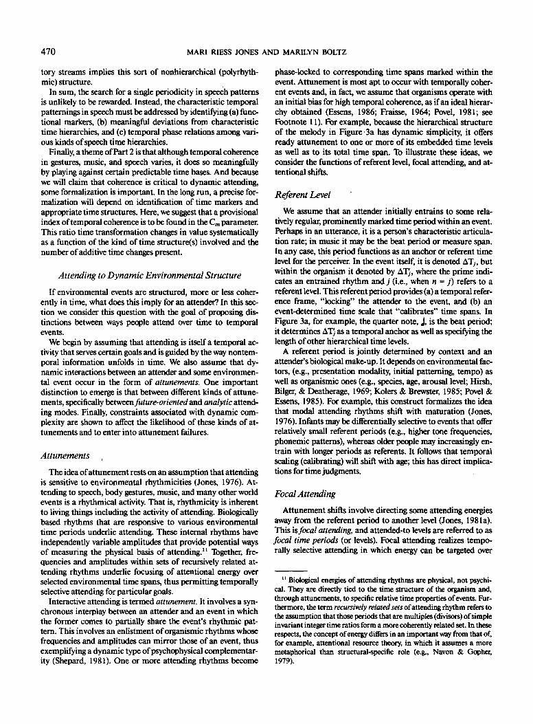
Figure 3 shows how differences in temporal coherence can come from variations in musical phrasing. Here, all timing changes concern relative phrase durations of a structural hierar- chy relative to fairly constant properties of a metrical hierarchy. Objectively, most coherence appears in Figure 3a in which both (binary) hierarchies coincide in time. Each measure opens with a metrical (stress) accent, and although the 8-beat melodic phrases are longer than measures, each resolves (h coupled with t accents) predictably at the end of alternate measures. This yields a single prominently marked time structure as in Figure 2a. By contrast, against the same metric frame, melodic phras- ing (signaled again by joint h and t structural accents) forms a less coherent time pattern (Figure 3b). This piece opens with regular and strongly marked melodic phrasings, but it closes with a musical surprise created by deviant phrase lengths of 6 and 10 beats, respectively. In this, it shares the format of Figure 2e. The psychological impact of such deviations is considered in later sections. Finally, even more temporal uncertainty is found in Figure 3c, in which a subtle modulation of the struc- tural hierarchy of Figure 3a occurs. In this case, the t accents remain hierarchical. In fact, they reinforce the metric time hier- archy. Notice that only harmonic accents are shifted to vary phrase durations. They alone create a nonhierarchical form.
In sum, musical coherence varies in meaningful ways that lend themselves to certain formalisms. We should underscore that we do not claim that the more coherent musical events are the more interesting or appealing ones; often they are not. Un- questionably, a certain level of artful and even systematic viola- tion (e.g., syncopation) of very coherent structures is necessary to create aesthetic appeal. We merely claim that these variations speak to temporal predictabilities. In this regard, coherence de- creases and dynamic complexity increases whenever simple time hierarchies are violated by additive time changes and/or by other temporally phased hierarchies.
failed to take account of anticipatory behaviors, and thus are not con- elusive.
Speech
Among other human songs intended to serve communication goals are those created by dynamically coordinated vocal ges- tures, namely speech patterns. Speech, like music, presents ap- parent rhythmicities that, on closer inspection, fail to lit the simplest time hierarchies. Again, the key to unlocking these timing mysteries may turn on the identification of appropriate time markers as well as clarification of different time structures and their interrelations.
English is a stress-timed language with appropriate time in- tervals thus defined between stress points. The simplest rhyth- mic pattern proposed for the distribution of stress points is iso- chrony, in which accents within unbroken utterances should be temporally equidistant (Pike, 1945). However, only limited empirical support exists for the isochrony principle even in a sophisticated version based on binary time hierarchies (e.g., Lehiste, 1976; Martin, 1972; Shields, McHugh, & Martin, 1974), thereby raising questions about its sufficiency (e.g., Lib- erman & Prince, 1977).
Some investigators argue that deviations from isochrony function meaningfully in communication (Lehiste, 1977). For example, spoken phrases are often marked by end lengthening and proportional silences as in music (Paccia-Cooper, & Cooper, 1981). Other meaningful deviations, stemming from shifts in speaker articulation rate, marker strength, and intonational contour can communicate emotional states (Scherer, 1979), in- tentions (Lehiste, 1976; Pickett, 1980), and turn-taking goals of speakers (Siegman, 1978; Wiemann & Knapp, 1975). In many cases, these deviations are additive time changes that derive con- textual meaning by violating the predictability conferred by un- derlying time symmetries.
Insight into underlying time symmetries is suggested by Cut- ler and Isard 0980). Using careful measurements of interstress intervals, acoustical manifestations of anisochrony were found to reveal an underlying invariant rhythm. Interstress intervals within a syntactic boundary are isochronous, maintaining a ra- tio of 1,00; however, the relative duration of adjacent intervals separated by a syntactic boundary is consistently lengthened to a ratio of 2:1. Cutler and Isard argued: "Increased duration results not from a complete disruption of isochrony, but rather from 'skipping a beat' so that the duration of longer intervals is twice that of shorter ones" (p. 258). Other evidence supports certain ratio timing properties in speech (e.g., Kozhenikov & Christovich, 1965; TuUer, Kelso, & Harris, 1983).
Thus, it appears that both temporal regularity and systematic deviations from regularity do exist in speech patterns. Never- theless, to align regularity simply with binary time structures based on stress markers is too restrictive for several reasons. First, even with stress-timed intervals, other time structures such as trinary and more complex hierarchical forms may be
mo Complex metric time ratios refer to C,n = ATJAT~_I, values that form nonintegers such as 6/4 and 9/8 (or compound meters, e.g., simple meters such as 2/2 6/4 multiplied by 3). Also, ratios that differ with respect to level--as in 3/4 meter, where Ct = 3 at one level and Ct = 2 at others--are only a slightly more complex time hierarchy. Metric ra- tios form either simple or complex invariants in time and thus provide the basis for specifying rhythmic patterns, as Jones (1981 a, 1987a) has shown.

O~.AMIC ~E .O . .O
a ) ~2 BEATs i .~ BEATS ,~ ~ATS
B BEATS B BEATS II B BEATS ~ BEATS II II II
Accent Type S M i M SIM [M SIM i M SIM i M S , O ~ . i . . . . . . . . . . . . i ~ , , [.,.." .~ ;Jrr~i J-~'.- ' : '
,cc.o,.'~' -'(?):-'-"' (~i' " - (?):- :"-('~i ~ "(:) Notes G B G B G
Hierarchical Time Structure Accents Coupled (~)
469
b ) I 16 BEATS 16 BEATS ]
8 BEATS 8 BEATS II 6 BEATS I0 BEATS
1] I] 11 ~ ? . s ~ ~ c c . o , . . ,M s,~ ,M S~ MS ~ M S ,.. ,. ^ ; . } . 2 ~ ], j l . . l , . ~ i , : ~ ' ~ . , 4 1 . " J!. J f-"i, ;'
- % : (~) (?) i~) . . . . . (ii Accents Notes G B G B G
Non-hierarchical Time Structure Accents Coupled (~,)
c)
Accent Type~..~, S
Acceots '~ ( ' Notes G
6 BEATS 8 BEATS ,, B BEATS I0 BEATS
M M S S M M M M M M S I I
, , w l = = = i , I . , . J =,,,~ . . , J I , l ' l ~ l h ' 1 , . t
(~,,., ( . ( t , "~I"" (h)lt) B G B G
Non-hierarchical Time Structure-h Accents Decoupled (h)(t)
Figure 3. Variations in temporal coherence that arise from differences in relative durations of melodic phrases. (Properties of a structural time hierarchy are changed, whereas those of the metric hierarchy are not. Most coherence occurs in (a) in which S and M hierarchies coincide because coupled S accents [t plus h] end each phrase and these also coincide with alternate measure endings. Less coherence occurs in (h) in which S accents [t plus h] are again coupled, but they create a nonhierarchical event. In (c), t and h accents are deeoupled via an additive time separation; the t accents remain hierarchical [dotted lines], whereas h accents mark nonhierarchieal time levels [solid lines].)
operative. Second, significant time markers other than ampli- tude changes (stress) are also critical in speech timing. Pitch and time accents function to outline recursively related melodic phrases and intonational patterns in speech much as they do in music (e.g., Bolinger, 1958; Fry, 1958; Ladd, 1986). Finally, just
as with metric and structural time hierarchies in music, two or more different time structures underlying speech rhythms can combine to support complex temporal accent phasings (e.g., Figure 2d). Fowler's (1983) suggestion that vowels and conso- nants are produced by separate but temporally phased articula-
470 MARI RIESS JONES AND MARILYN BOLTZ
tory streams implies this sort of nonhierarchical (polyrhyth- mic) structure.
In sum, the search for a single periodicity in speech patterns is unlikely to be rewarded. Instead, the characteristic temporal patternings in speech must be addressed by identifying (a) func- tional markers, (b) meaningful deviations from characteristic time hierarchies, and (c) temporal phase relations among vari- ous kinds of speech time hierarchies.
Finally, a theme of Part 2 is that although temporal coherence in gestures, music, and speech varies, it does so meaningfully by playing against certain predictable time bases. And because we will claim that coherence is critical to dynamic attending, some formalization is important. In the long run, a precise for- realization will depend on identification of time markers and appropriate time structures. Here, we suggest that a provisional index of temporal coherence is to be found in the Ctn parameter. This ratio time transformation changes in value systematically as a function of the kind of time structure(s) involved and the number of additive time changes present.
Attending to Dynamic Environmental Structure
If environmental events are structured, more or less coher- ently in time, what does this imply for an attender? In this sec- tion we consider this question with the goal of proposing dis- tinctions between ways people attend over time to temporal events.
We begin by assuming that attending is itself a temporal ac- tivity that serves certain goals and is guided by the way nontem- poral information unfolds in time. We also assume that dy- namic interactions between an attender and some environmen- tal event occur in the form of attunements. One important distinction to emerge is that between different kinds of attune- ments, specifically between future-oriented and analytic attend- ing modes. Finally, constraints associated with dynamic com- plexity are shown to affect the likelihood of these kinds of at- tunements and to enter into attunement failures.
Attunements
The idea ofattunement rests on an assumption that attending is sensitive to environmental rhythmicities (Jones, 1976). At- tending to speech, body gestures, music, and many other world events is a rhythmical activity. That is, rhythmicity is inherent to living things including the activity of attending. Biologically based rhythms that are responsive to various environmental time periods underlie attending. These internal rhythms have independently variable amplitudes that provide potential ways of measuring the physical basis of attending, tl Together, fre- quencies and amplitudes within sets of recursively related at- tending rhythms underlie focusing of attentional energy over selected environmental time spans, thus permitting temporally selective attending for particular goals.
Interactive attending is termed attunement. It involves a syn- chronous interplay between an attender and an event in which the former comes to partially share the event's rhythmic pat- tern. This involves an enlistment of organismic rhythms whose frequencies and amplitudes can mirror those of an event, thus exemplifying a dynamic type ofpsychophysical complementar- ity (Shepard, 1981). One or more attending rhythms become
phase-locked to corresponding time spans marked within the event. Attunement is most apt to occur with temporally coher- ent events and, in fact, we assume that organisms operate with an initial bias for high temporal coherence, as if an ideal hierar- chy obtained (Essens, 1986; Fraisse, 1964; Povel, 1981; see Footnote 11). For example, because the hierarchical structure of the melody in Figure,3a has dynamic simplicity, it offers ready attunement to one or more of its embedded time levels as well as to its total time span. To illustrate these ideas, we consider the functions of referent level, focal attending, and at- tentional shifts.
Referent Level
We assume that an attender initially entrains to some rela- tively regular, prominently marked time period within an event. Perhaps in an utterance, it is a person's characteristic articula- tion rate; in music it may be the beat period or measure span. In any case, this period functions as an anchor or referent time level for the perceiver. In the event itself, it is denoted ATj, but within the organism it denoted by A~, where the prime indi- cates an entrained rhythm and j (i.e., when n = j) refers to a referent level. This referent period provides (a) a temporal refer- ence frame, "locking" the attender to the event, and (b) an event-determined time scale that "calibrates" time spans. In Figure 3a, for example, the quarter note, J, is the beat period; it determines A T as a temporal anchor as well as specifying the length of other hierarchical time levels.
A referent period is jointly determined by context and an attender's biological make-up. It depends on environmental fac- tors, (e.g., presentation modality, initial patterning~ tempo) as well as organismic ones (e.g., species, age, arousal level; Hirsh, Bilger, & Deatherage, 1969; Kolers & Brewster, 1985; Povel & Essens, 1985). For example, this construct formalizes the idea that modal attending rhythms shift with maturation (Jones, 1976). Infants may be differentially selective to events that offer relatively small referent periods (e.g., higher tone frequencies, phonemic patterns), whereas older people may increasingly en- train with longer periods as referents. It follows that temporal scaling (calibrating) will shift with age; this has direct implica- tions for time judgments.
Focal Attending
Attunement shifts involve directing some attending energies away from the referent period to another level (Jones, 1981a). This is focal attending, and attended-to levels are referred to as focal time periods (or levels). Focal attending realizes tempo- rally selective attending in which energy can be targeted over
'~ Biological energies of attending rhythms are physical, not psychi- cal. They are directly fled to the time structure of the organism and, through attunements, to specific relative time properties of events. Fur- thermore, the term recursively related sets of attending rhythm refers to the assumption that those periods that are multiples (divisors) of simple invariant integer tirne ratios form a more coherently related set. In these respects, the concept of energy differs in an important way from that of, for example, attentional resource theory, in which it assumes a more metaphorical than structural-specific role (e.g., Navon & Gopher, 1979).

DYNAMIC ATTENDING 471
some time levels and not others to serve certain goals (Jones, Boltz, & Kidd, 1982; Jones, Kidd, & Wetzel, 1981; Neisser & Brecklen, 1975). For example, if a listener's goal is to "catch" the global idea of a speaker, attending will be targeted over higher focal time periods in an utterance than if the listener must concentrate on the speaker's vowel pronunciation. Be- cause focal attending involves energy shifts, it is more etfortful with dynamically complex events and with attunements to pro- portionately smaller time periods (higher frequencies).
How does shifting occur?. It relies upon the attender's use of time transformations. Formally, let a primed interval, ATn, re- flect the attending rhythm that becomes attuned to level ATn in the event. Focal attending reflects the phase-locking of "In with AT'n, in which ATn = AT'n for a subset of levels. The phrase using time refers to a reliance on an extracted time rule (e.g., C;) to shift attending energy from one level to another. Any at- tending level, AT'n may therefore be a focal level if it gains en- ergy. A focal level is related to a referent period by a time rule, (C~) n-j. This is evident in the following recursive formula:
ATn = ATAC~) "-j (where In - J l < 5). (2)
To the extent that C~ and T~ are good estimates of C~ and ATj in the event, then AT" = ATn.
People can rarely verbalize use of a rhythm generator (C~), nor can they report focal time levels (AT'n; Jones, 198 la). Focal attending is a tacit, how-to skill that is implicitly acquired (Re- ber, Kassin, Lewis, & Cantor, 1980).
Attentional Shifts
An important aspect of skilled attending and expertise is flexibility (e.g., Gentner, 1987; Keele & Hawkins, 1982). Flexi- ble attending here refers to shifts of attending energies from the referent level to many other event levels. For example, in the event of Figure 3a, a skilled attender can use ratio time invari- ants to flexibly target multiple time levels, moving effortlessly from one to another to serve different needs. Thus, if a person is attending over melodic phrases (e.g., 4 and 8 beats) but must respond to some higher level, that person may easily transfer more attending energy over this level (e.g., 16 beats) or even the entire event span by relying on Equation 2. In short, attunement shifts allow one to selectively "examine" strings of notes mark- ing a given hierarchical level.
One of us has suggested that flexible attending offers a practi- cal solution to the problem ofstructural ambiguity and the fact that a given event means different things in different contexts (Jones, 1986; see also Cutting, 1982). Depending on the task, a person can rely on high or low focal levels to attune to event relationships most relevant to some function. In fact, we distin- guish two general kinds ofattunements. Future-orientedattend. ing involves a global focal attending over time periods higher than the referent level (n > j), whereas analytic attending directs attending energies to relatively low levels in a temporal hierar- chy (n < j ) . Thus, future-oriented attending may support one's ability to follow conversational turn-taking between two speak- ers, and analytic attending would underlie identifying the dia- lect of one of the speakers. These focal attendings rest on differ- ent temporal perspectives of the same event.
These attending modes involve different regions in a contin- uum of nested time levels, but with the following two qualifica-
tions: (a) that they yield different temporal perspectives on the same event relative to a given referent level associated with that event (higher for future-oriented, lower for analytic), and (b) that they may support selectively different sorts of activities, de- pending on task goals. That is, future-oriented attending is par- ticularly functional when longer term preparatory attending and real time extrapolations of an unfolding event are involved. A future-oriented extrapolation is termed an expectancy. Ana- lytic attending is more functional when relatively short-term ac- tivities are involved. Because relevant focal periods are usually less than that of the referent period, expectancies as such are not supported, although attending to local detail and grouping with respect to the referent span is.
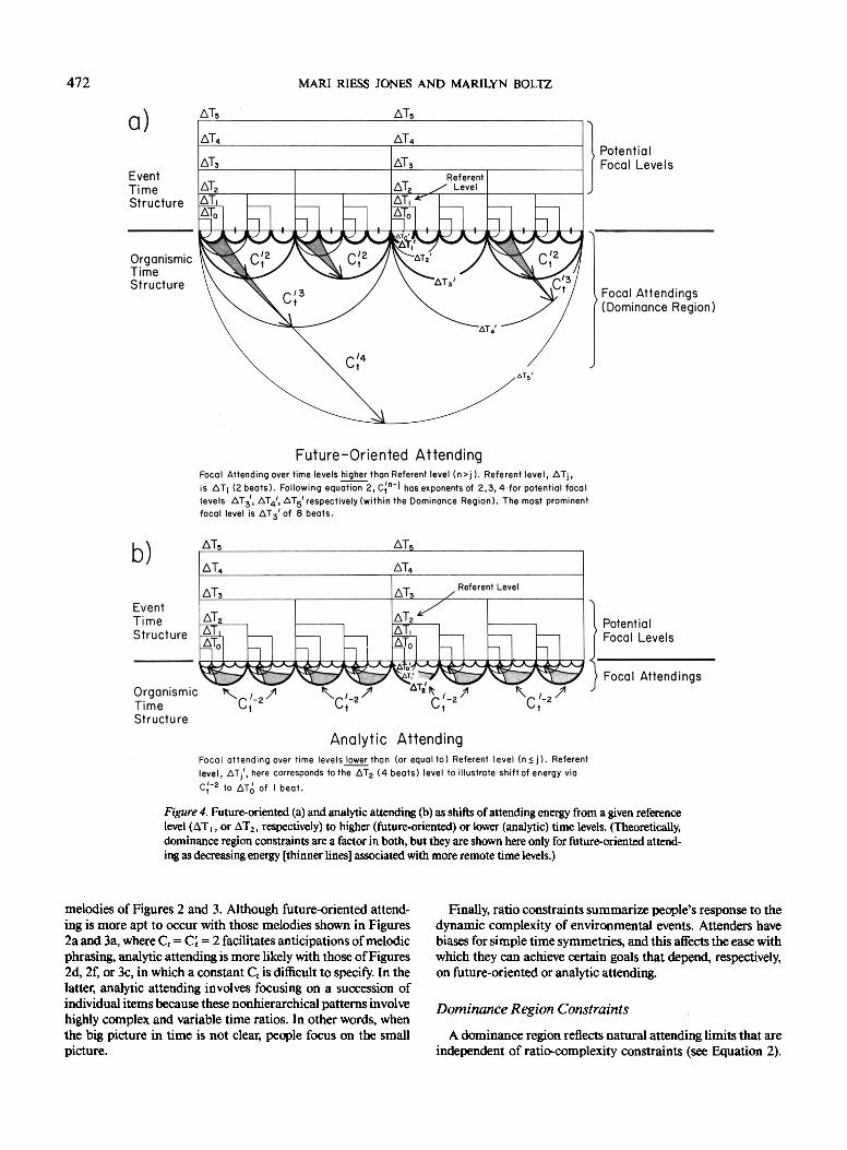
Figure 4 illustrates that both attending modes are possible in a coherent event. They are shown here with different referent levels (for comparison purposes, both are standardized with re- spect to the same beat period). In Figure 4a, future-oriented attending involves shifts up to several potential focal levels higher than the referent, which here is a two beat period (n = j = 1). The AT3 focal level receives most attending energy (C; n-j = 22), so that future tonal onsets separated by 8 beats are readily anticipated, although final endings are also predictable (via C~ = 24). Future-oriented attending occurs here because Ct = 2 may be extracted and used recursively as C~ (where C; = C,).
In Figure 4b, the referent level becomes four beats (n = j = 2) in order to illustrate analytic attending. With this attending mode, energy can be shifted down to the level of adjacent items or pulses (AT0) from AT2. Thus, when someone attends analyti- cally, attending is focused downward to cover fine changes that transpire over relatively small time periods (including the refer- ent period). Such an activity might correspond, for instance, to tracking or even to counting these elementary items in groups of four. It can be effortful and will be more common in early stages oflearning~
Constraints on Attunements and Attunement Shifts
A person's goals determine time levels most relevant for at- tunement. But the catch is that although attunements to an event can shift to achieve different goals, the event's dynamic complexity will constrain the ease with which this is accom- plished. In particular, attunement shifts are less likely in events of low temporal coherence. This idea is formalized as a con- straint on attunement conferred by the event's ratio time prop- erties (ratio complexity constraint). Other constraints on at- tunement exist but these concern the attender's inherent ability to shift attending (dominance region constraints).
Ratio Complexity Constraints
Attunements have been described with reference to highly coherent events, ones that confirm a bias for simple time ratios. The complement of this bias represents ratio complexity con- straints. With less coherent events, attending becomes less flex- ible (at least initially) because the ratio, Ctn, is complex. Attend- ing is confined to one or two temporal levels in which biases for simple and constant ratios may be realized. In short, analytic attending is more likely with many nonhierarchical events.
To illustrate, consider the ways of listening encouraged by
472 MARl RIESS JONES AND MARILYN BOLTZ
Figure 4. Future-oriented (a) and analytic attending (b) as shifts of attending energy from a given reference level (ATe, or AT2, respectively) to higher (future-oriented) or lower (analytic) time levels. (Theoretically, dominance region constraints are a factor in both, but they are shown here only for future-oriented attend- ing as decreasing energy [thinner lines] associated with more remote time levels.)
melodies of Figures 2 and 3. Although future-oriented attend- ing is more apt to occur with those melodies shown in Figures 2a and 3a, where C, = C; = 2 facilitates anticipations of melodic phrasing, analytic attending is more likely with those of Figures 2d, 2f, or 3c, in which a constant Ct is difficult to specify. In the latter, analytic attending involves focusing on a succession of individual items because these nonhierarchical patterns involve highly complex and variable time ratios. In other words, when the big picture in time is not clear, people focus on the small picture.
Finally, ratio constraints summarize people's response to the dynamic complexity of environmental events. Attenders have biases for simple time symmetries, and this affects the ease with which they can achieve certain goals that depend, respectively, on future-oriented or analytic attending.
Dominance Region Constraints
A dominance region reflects natural attending limits that are independent of ratio-complexity constraints (see Equation 2).
DYNAMIC ATTENDING 473
Even with simple hierarchical time patterns, attenders can only shift attending energies so far before the connection between an established referent and a remote focal level breaks.
Specifically, the dominance region involves a set of related time levels around the referent beat period, It reflects the distri- bution of predominant attending energies over hierarchically neighboring time levels (a related concept is the serial integra- tion region; Jones, 1976). 12 For example, in musical composi- tions in which many related time levels appear, the dominance region suggests that attending shifts from a referent to remote levels are unlikely; listeners cannot accurately anticipate the length of a symphony from its tempo. (A similar notion is tac- tus, a perceptually dominant subset of time levels surrounding the musical beat; Lerdahl & Jackendoff, 1983). Dominance re- gion time levels (ATb to ATs) are suggested by potential focal levels shown in Figure 4a. The key notion is that attunements shifts exceeding [ n - J l of 4 or 5 become increasingly difficult.
Dominance region limits are relative not absolute time limits in that they are expressed in terms of hierarchical levels (expo- nents ofC~). Attunements are relative to an event's characteris- tic referent period, meaning that one can potentially attend over a limited set of related time levels, regardless of their absolute time values. But note that if attenders are strongly biased in entraining to a given referent period, then these relative con- straints will seem like absolute ones. Concretely, this means that perceived coherence can be affected by a pattern's rate or dura- tion.
Failed Attunements
Given the preceding discussion of attunement constraints, it follows that attunements can fail. A failed attunement is an asynchrony between some attending rhythm (AT'n) and the rele- vant focal level of an event (ATn). The nature and consequences of such asynchronies will differ as a function of event complex- ity. That is, in less complex events there will be fewer attune- ment failures and a given temporal asynchrony can stand out as a temporal contrast based on future-oriented attending. In highly complex events, many asynchronies appear and these force attunement refinements based on analytic attending.
tofferson, 1976).13 Here, we propose that certain contrasts can influence judgments about events when the goal is time estima- tion.
Refining Attunements and Analytic Attending
Complex events contain many irregularities, and so they in- evitably invite many failed attunements. In the face of this, re- doubtable attenders may turn to refining attending skills de- pending on the nature of the task. Indeed, if the event is based on a complex time hierarchy, this implicit learning can lead to the discovery of initially obscure temporal invariants. However, with nonhierarchical events in which no invariant time rule ex- ists, such skill acquisition is less likely. For instance, the pattern of Figure 2f affords little opportunity for flexible attending, ei- ther initially or with practice. Here, ratio constraints on attend- ing mean that attunements will be confined to one or two lower time levels where they may support various goal directed activ- ities.
Summary of Part 2
Dynamic attending reflects the attender's tacit use of an event's dynamic structure. It relies on the particular nature of the event's temporal invariants (e.g., in gestures, music, speech), which if present, determine its coherence or conversely its dynamic complexity. Because environmental events differ in coherence, they offer the rhythmical attender different ways to selectively synchronize with one or more nested time level(s) (focal attending) to achieve specific goals. This participatory attending is termed attunement and is temporally selective. At- tunement involves entrainment to a referent time period and selective focal attending to some time level. Attunements are flexible. They can shift over focal levels to reflect either future oriented or analytic attending. However, this flexibility is lim- ited by ratio complexity constraints related to rhythmic invari- ants and by dominance region constraints related to the span of an attunement shift. Consequently, future-oriented attending that permits expectancies about event endings is more likely with coherent events, whereas analytic attending that encour-
Temporal Contrast and Future-Oriented Attending
Imagine anticipating the shape of an unfolding event and finding to your surprise that there's a discrepancy. This is what occurs whenever a nonhierarchical event begins deceptively as a hierarchical one. The melody of Figure 3b does this. Initially, it supports future-oriented attending, but as we saw earlier, it carries the potential for a musical surprise because finally it de- viates from its opening regularity. Formally, this yields an ex- pectancy violation: One expects a certain future time course (i.e., C~ = 2), which does not occur. The difference between ob- served and expected focal periods at some level, n, represents an asynchrony that is experienced as a temporal contrast: ATn - AT'n. We assume that temporal contrast determines one's response (e.g., surprise) to systematic additive changes (asymmetries) that play against time symmetries. In short, it is contrasts of various sorts that function to communicate rhyth- mic styles, emotion, and time change. And something akin to temporal contrast may function in time discrimination (Kris-
~2 The serial integration region addressed the way in which temporal order is preserved in world events through relationships between proper- ties of markers at different time levels. For example, if at level n, the pitch change over that level--namely, AP,--is disproportionately great for the corresponding time change--namely, ATn--then the pattern will have low temporal coherence. A consequence is the breakdown of syn- chronous attending and loss of one's ability to order things in time. This is evident in phenomena such as auditory pattern streaming (Jones, 1976). The serial integration region, thus, is bounded by extreme pitch/ time (APn/ATn) ratios. It is contained in the dominance region, which is bounded by extreme time/time (ATn/ATj where In - J l = 4 or 5) ratios. In this article we focus only on constraints affecting time levels, that is, dominance region constraints.
~ Temporal contrast and lawful patterns of temporal contrasts serve special communicative functions in music. Jones (1987a) has suggested that these additive time changes arise from a horizontal component in- troduced into a performer's production patterns, a component that cor- responds to velocity patterns of gestures. In other contexts, singular con- trasts defined earlier, have been postulated to affect time discrimination (Kristofferson, 1977).

474 MAR1 RIESS JONES AND MARILYN BOLTZ
ages focusing over lower time levels is more likely with less co- herent events. Finally, attunement failures can lead to temporal contrast, namely the deviation of expected from observed focal levels.
Part 3: Dynamic Attending and Time Estimations
The conceptual framework of Part 2 has implications for at- tending in various contexts. Part 3 develops these with respect to time estimation. Solutions posed with regard to the filled in- terval effect (Part 1) are seen as consequences of constraints on a general attending activity imposed by these tasks. One goal of Part 3 is to model time estimation behaviors in comparative judgment and production tasks using general assumptions of dynamic attending.
Typically, a time estimation task requires assessment of one or several time intervals. In light of Part 2, this creates a puzzle: If people attend rhythmically, by relying tacitly on ratio time transforms, then how do they come to explicitly judge time in- tervals as such? Society and our own schedules require that we judge time as intervals, and we often comply with more or less accuracy. How is this puzzle resolved?
One resolution plays on the idea that interval time estimates encourage selective attending over higher order time spans that relate beginnings and endings of judged events. Clearly, this at- tending has a basis in relative time. Yet, the interval time esti- mate is not necessarily an easily achieved goal. The perspective of Part 2 suggests three assumptions about the way rhythmical attenders approach such tasks: (a) They use relative time to achieve task goals. (b) Ease of goal achievement depends on event structure, notably on the way dynamic complexity con- strains flexible attending (i.e., future-oriented and analytic). (c) Time estimates themselves depend on tacit use of resultant fo- cal levels and because awareness of these levels is poor, time estimates are liable to be biased by attunement failures (tempo- ral contrast and attunement refinements).
According to the first assumption, interval time requests en- courage attenders to target attending over one or more higher time levels (future-oriented attending). In the second assump- tion, their success depends on event complexity. Future-ori- ented attending is easier to achieve in comparative time judg- ments about simpler time structures. Here, expectancies about ending times of standard and comparison events are fairly effortless. Finally, according to the third assumption, if an at- tunement failure occurs, then it creates a temporal contrast, and this, in turn, is apt to tacitly bias time judgments especially if ending times are involved. That is, people respond to the pres- ence or absence of expectancy violations, not to absolute values of expected intervals. This scenario predicts that people can correctly judge intervals whenever a comparison event truly ends before (or after) some expected ending time (given by the standard). By the same token, it predicts that people will err in judging truly identical intervals if one (or both) event(s) hap- pens to violate expectancies about event endings (a filled inter- val effect). This occurs whenever expectancies based on embed- ded, not total, time periods lead to contrasts that implicate an event's ending. If these embeddings make an event's ending seem too early or too late, then time judgments can be tacitly distorted. Contrasts do not occur with expectancy confirma- tions nor when either the expected or observed time period is
absent. But when they do occur and impinge on ending times, then biased time estimates can result. In sum, one way rhythmi- cal attenders cope with time intervals depends on fnture-ori- ented attending and temporal contrast.
If attenders don't succeed in attending over higher time levels, then analytic attending occurs. In this case, although interval time estimates remain influenced by the way information fills to-be-judged time intervals, biasing can take a different form. Particularly if events are incoherent, whenever task goals bring into play memory-oriented strategies, attending will be focused over lower time levels. People may engage in counting, grouping, associative labeling, and so on, in order to impose some struc- ture on the event, and all of these activities direct attending to relationships among adjacent items. Consequently, if time esti- mates are required they will be biased by these activities and specifically by differences in focal levels used to attend to the events involved. For example, if two complex tunes of equal duration are filled with different numbers oftones, then the one with more tones will usually involve a denser temporal spacing. If people count tones, then attunements to the denser sequence will be based on lower focal attending. However, awareness of focal time levels is poor. Thus, whenever people tacitly (and er- roneously) infer that focal levels used to attend to each tune are the same and that the one with more tones is longer, then judgment errors will appear (a filled interval effect). Again, such mistakes arise from the attenders' lack of awareness of differ- ences in focal levels actually used. In sum, a second way in which rhythmical attenders cope with intervals of time involves focal time level differences based upon analytic attending.
In short, Part 2 suggests a broad dichotomy for the way rhyth- mical attenders interact with temporally coherent and nonco- herent events, and ultimately this explains how they may arrive at interval time estimates. Independent evidence for this dis- tinction comes from Povel and Essens (1985), who found that reproductions of hierarchical auditory sequences involve a reli- ance on higher order time relations, whereas those of nonhierar- chical sequences involve the use of mnemonic strategies such as counting (see also Bamberger, cited in Povel & Essens, 1985; Hamilton & Hockey, 1974; Jackson, 1985; Maser, 1983). This distinction offers a way of explaining the notorious variability found in time estimation studies. It suggests that duration esti- mates of the same event will vary with attending mode.
Finally, although this framework relies on new constructs such as future-oriented and analytic attending, the analytic at- tending mode does incorporate notions underlying contempo- rary time models. It differs in linking the mnemonic activities suggested by current time models to a rhythmic base and to differences in focal time levels. Thus, it suggests that although attending to events filled with more information may involve more effort (Underwood & Swain, 1973) or complexity (Ornstein, 1969) or changes (Block, 1978), finally the decisive factors involve temporal levels of attending.
Time Estimation in Judgment Tasks: A Contrast Model
A contrast model formalizes the proposal that time judg- ments are biased by the style of attunement failure (temporal contrast or mnemonic refinements) associated with a given at- tending mode (future-oriented or analytic). Two parameters of this model reflect contrast and mnemonic activities, respec-

DYNAMIC ATFENDING 475
tively. A third parameter, a coherence weight, determines the likelihood of either attending mode. It reflects ratio complexity constraints (Part 2) and so summarizes the impact of dynamic complexity on attending.
In comparative duration tasks, the temporal contrast biasing time estimates is a pairwise one based on expectancy violations in both events; for pair i it is denoted by the parameter, DE/. The mnemonic difference parameter is based on differences in analytic attending levels over both events; it is denoted DM/. Here, we apply the model to filled time intervals that are equal in duration but extensions to unequal intervals are straightfor- ward and given in the Appendix. Thus, for any pairwise judg- ment, i, we assume that two kinds of random variables exist that are distributed, respectively, as N(DE/, ~i2) and N(DMi, aMi2), in which aEi 2 = aM 2 = o'i 2.
Formally, the Contrast Model differentially weights temporal contrast, DE/, and mnemonic differences, DMi, by the proba- bility of future-oriented, W/, and analytic attending, 1 - W/ (0 < W / < 1.00). This logic leads to a binary mixture modeling of the two attending states (Townsend & Ashby, 1983). Let D~ be the expected value of a theoretical distribution of duration estimates that results from a binary weighting of the two states:
Di = WIDE/+ (1 - Wi) DMi. (3)
The predicted average of scaled duration judgments, JD/, is a monotonic function, f, of D/. For simplicity, f is assumed to be linear with scale parameters a and b. The intercept parameter, b, reflects response scale category; if b is the score for a null difference judgment, then average judged time magnitudes in a rating task are as follows:
JDi = f[Di], (4)
and
JD/= a[W/DEi + (1 - W/)DM/] + b. (5)
Judgment bias is given by the point of subjective equality, PSE/, and is gauged for the case in which two intervals have identical total durations. From Equation 5, the contrast model predicts PSE/as follows:
PSEi = JDi - b = a[WiDEi + (1 - W/)DM/]. (6)
The predicted variance of observed duration judgments is de- rived from assumptions regarding moments of the weighted dis- tributions. This is SD~ 2 for judgments of event(s) i:
SDi 2 = a2[Wi(l - W i X D E i - DMi) 2 + ai2]. (7)
Equations 5-7 reflect predictions of the contrast model. They show that mean judgments, bias, and variance are a function of the weighting parameter, W/, and the two attending mode parameters, DE/, and D M i .
Parameters and Their Estimation
The W/ weight is sensitive t o environmental structure, whereas the DE~ and DM/attending parameters reflect the re- spective impacts of attending mode on time estimates. Parame- ter determinations rest on the attunement constraints described in Part 2. In particular, following the dominance region con- straint, we assume that embedded periods play an important
role in guiding attending over pairs of events in comparative judgments. And with respect to ratio complexity, we assume that Ctn determines the value of the coherence parameter, W/, over both events. We now illustrate parameter determination using the hierarchical and nonhierarchical musical examples of Figure 3 to fill standard and comparison time intervals.
The Weighting Parameter, W~
The W/parameter is identified with conditions that deter- mine whether one uses analytic or future-oriented attending for time estimation. The most important of these is the temporal coherence of the events to be judged. Thus, assume that hierar- chical (H) and nonhierarchical (NH) melodies fill standard and comparison intervals as shown in Figure 5 (H - NH or NH - H). Temporal coherence is greater when H melodies are in- volved and also when they function as standards. In these cases, dynamic complexity is low and hence W/should be high. Thus, W/is high when Ct, for situation i is an invariant and low integer ratio. In other words, estimates of W/, '~/, should be higher with (a) H events (than NH ones), and (b) pairwise comparisons of the form H - NH (than NH - H). Finally, instructions and task demands (goal/function) can also affect W~ by determining the likelihood of a given attending mode.14
Attending Mode Parameters
In principle, although either attending mode is possible for a given event, they are not equally likely. Furthermore, because each mode is associated with its own brand of attunement fail- ure, different time estimates can occur for the same situation. This is important because it reinforces the point that the way people attend influences their time estimates. We show this us- ing two melodies filling identical time intervals.
Estimation of DE~. If people attend in future-oriented ways to events of Figure 5, the X will be biased by a pairwise contrast, DE/. Estimates of DE~ (DE/) are based on individual temporal contrasts in each event. Individual and pairwise contrasts at any level can be positive, negative, or zero. If contrasts involve the total time level of each event, then truly unequal time intervals obtain (see Appendix). But if they arise from time levels embed- ded within events of equal duration, as shown in Figure 5, then contrasts based on final embedded periods determine DE~. Thus, DE~ is a difference of final contrasts, AT 0 - AT~o, from each o f j patterns ([j = 1, 2] level subscripts suppressed). This parameter reflects a comparability of expectancy violations across both patterns:
DEi = (ATa - AT,2) - (AT/, - AT,-1). (8)
14 Comparative judgment tasks have traditionally been distinguished in terms of prospective and retrospective designs. Such d e s i g n differ- ences can also influence Wj. In prospective tasks, people are told to compare the durations of two forthcoming intervals leading to a greater chance of future-oriented attending. In retrospective tasks, people en- gage in incidental activities during two time spans ot~en based on ana- lytic attending; later they learn they must compare durations. This vari- able contributes to divergence in the literature in that differential results between task type sometimes occur (e.g., Block, George, & Reed, 1980; S. W. Brown, 1985; Hicks, Miller, & Kinsbourne, 1976). We believe this mixture of results comes from interactions of instructions with event coherence.

476 MARI RIESS JONES AND MARILYN BOLTZ
a) H STANDARD)
AT ,
AT;= = 8 beats
( A T I I - AT l l l } = 0
A
NH (COMPARISON)
.__, 8+8+10 - - - ,~,T i:, = "-- ' - -~- '~ : ~ . b r
~ E AT i2 = 6 b e a t s
(T i2 - Z~T~ a ) = (6 - 8 . 6 7 ) = - 2 . 6 7
DE I = (AT~z- AT'Iz)-O =-2.67 ( Negative Contrast)
b) NH H (STANDARD) (COMPARISON)
I 8+8+10 I ~ T I I 2 = 8 beats I ZXT , , = - - T - - = s.67J,
I I ~-k~-~l,_L-~_ko_i . . . . . . . . . . . . . . . . ° , ~'l,_ Lo _~'~l, _ L ° _ h _L o_ ~-~ _ Lo _~
A T i l = 6 beats A T i 2 = 8 beats
( A T I I - A T I ; I ) = ( 8 . 6 7 - 6 ) = 2 . 6 7 (ATi~ , - AT/12) = 0
A DE I = O-(ATi i-AT' i i ) = +2.6"/' (Positive Contrast)
Figure 5. Abstracted time structures for two events, a hierarchical (H) and a nonhierarchical (NH) one, to be judged in a comparative time estimation task. (This event pair i produces two different kinds of temporal contrast, DEi, depending on event order. In (a) the H melody is the standard and the NH is the comparison yielding a negative contrast. In (b) the NH is the standard and the H is the comparison, yielding a positive contrast. These time structure represent the melodies of Figure 6. Smaller dots represent a common beat period and larger dots signify superordinate time periods of phrases marked by S accents. Expected ending time is denoted by E.)
Equation 8 simplifies whenever an expectancy about one pat- tern ending is confirmed because that contrast becomes zero. Thus, if the first pattern ( j = 1) of pair i confirms an expected ending time, then ATh = AT, and
DEi = ATi2 -- ATe2. (9)
Different degrees and kinds of pairwise contrasts are given by Equations 8-9. For example, strong expectancies over the H - NH arrangement (Figure 5a) should appear because C~ = 2 and a common referent period (quarter note) obtains for both events. Anticipations, reinforced in the standard, will occur in the comparison for focal periods of 8 beats or more (i.e., AT'a is the average duration of preceding phrases in the comparison: AT'n = (8 + 8 + 10)/3 = 8.67 beats). This expectancy is ulti- mately violated in the comparison in which a final tonic occurs too early (after 6 beats), yielding a negative pairwise contrast of I)E i = -2 .67 beats (Equation 9). Reversing the order of H and NH events (Figure 5b) leads to a positive pairwise contrast of the same magnitude (I)E i = 2.67). More generally, Equations 8-9 indicate that the magnitude and direction of any pairwise contrast depend on discrepancies between observed and ex- pected endings within both patterns.
Estimation of DM~. If people attend analytically to these same events, they are biased by DM~. This may apply if people resort to countingAlower order features within each event. Esti- mates of DM~ (DM ~) will not necessarily agree with contrast
estimates (I~E i). If DMi is based on a counting strategy, then let N li and N2~ denote, respectively, the number of items, chunks, or beats that are counted within the i th pair of standard and comparison events at the focal levels used. We assume that people often tacitly infer that associated analytic attending lev- els are the same for both events; this common focal level is de- noted by A ~ (suppressing level subscripts). Thus, DMi is esti- mated by
DMi = AT~(N2i- NIi). (10)
For example, if attending is confined to the referent level, then DMi is estimated from differences in the number of beats counted in each event. In the events of Figure 5a and 5b, the assumption o f equivalent focal periods is correct and so cor- rectly yields DM ~ = 0, because N 1 i = N2~. But, whenever beats (or other attended-to information) mark out different N 1~ and N2~ values, this assumption is incorrect. Consequently, time distortions are predicted (filled duration effect). Supporting evi- dence for Equation 10 applied to beat counting is found in stud- ies showing that time estimates are systematically biased when people judge melodies having identical durations but different total numbers of beats (N1 :~ N2); Boltz, 1985). 15
15 Boltz (1985) found that when two melodies are identical in dura- tion, as well as in number of tones and number of pause-defined chunks, they are nonetheless judged to differ in duration as a function of the number of different beats, with those containing more beats judged to be longer.

DYNAMIC ATTENDING 477
In sum, attending mode parameters can assume different val- ues for the same pair of events. Furthermore, either parameter can yield over- or underestimations of a given interval. The de- gree to which one or another parameter estimate holds sway depends on its relative weight (Equations 5-7). Temporal con- trast effects will predominate if future-oriented attending oc- curs (high W~), whereas mnemonic differences will predomi- nate if analytic attending occurs (low W~). In general, this leads to predictions that variability and disagreements in time esti- mates are to be expected. Explanatory orderliness comes only with reference to event structure and dynamic attending.
Contrast Model Predictions
The Contrast Model predicts that judgment accuracy (Equa- tion 5), average bias (Equation 6), and variance (Equation 7) will vary systematically with model parameters. Among its im- portant predictions are the following: (a) Time estimates will be biased in magnitude and direction by values of contrast (DEi). (b) Biasing effects of a given contrast will increase directly with temporal coherence, namely with increments in Wi. (c) Esti- mates of Wi will be a function ofpairwise coherence, as indexed by Ct,, such that XfCi will be high whenever a pair contains H patterns and especially when these serve as standards (ratio complexity constraints). (d) Judgment variability should de- crease with increasing predominance of one attending mode (as Wi --* 1.0 or 0.0).
Numerous other predictions can be deduced from Equations 5-10. Some concern effects of mnemonic strategies (DM~), which should be most pronounced when Wj is low. Others con- cern range effects arising from dominance region constraints. Finally, additional parameter influences on judgment variance can be anticipated from Equation 7.
These same equations also generate corresponding predic- tions about judgment accuracy and discriminations of unequal time intervals. These appear in the Appendix where related models such as Kristofferson's (1977) real time criterion model are considered. Systematic departures from Weber's function are predicted by the Contrast Model as a function of task, at- tending mode, skill, and event structure. However, our focus here and in Part 4 is on the case of equal time intervals and in particular on the first several predictions previously outlined.
Time Estimation in Production Tasks: Expectancies
The Contrast Model only applies to comparative judgment situations. But time estimation has also been studied in tempo- ral reproduction and production tasks (cf. Allan, 1979; Baker, 1962; Bartlett & Bartlett, 1959; Johnson, 1986; D. N. Lee, 1980). In reproduction, subjects recall a time span by overtly marking its beginning and end. In production, a specified span (e.g., 1 s) is constructed. A variant of the latter involves timed extrapolations in which part of an interval is presented and the appropriate remaining time must be produced. Analyses of re- production and production tasks are beyond the scope of this article. However, temporal extrapolations are relevant because they directly involve expectancies.
Temporal extrapolations require an individual to use the pre-
ceding context to indicate (overtly) when an event should end in real time. Thus, they have potential for revealing expectancies because only the initial part of an event occurs and one must covertly continue it. Attending that controls performance oc- curs in the absence of the event itself; only "pure" expectancies remain.
Predictions based on expectancies rely on Equation 2. As- suming that a referent period, ATj and a rhythmic generator, C't, are supplied by the preceding context, Equation 2 suggests the existence of sets of nested expectancies. Let AT" be the value of that focal period most relevant to a particular task. Produced and extrapolated times reflect such expectancies, and these can be predicted from average values of AT, within the relevant event. Thus, focal periods of 8 beat phrases within a musical event allow estimation of the extrapolated completion time, providing, of course, that the listener uses expectancies to time extrapolations. By contrast, analytic attending should not pro- duce extrapolation times that are systematically related to an event's higher order time periods.
Summary of Part 3
Time estimation in judgment and production tasks involves dynamic attending over various levels of structure within events that fill time intervals. According to the Contrast Model, means and variances of comparative duration judgments are deter- mined by the likelihood of different attending modes (future- oriented, analytic) and their related potentials for attunement failure (temporal contrast, mnemonic activity). Over- and un- derestimates can occur with either future-oriented or analytic attending, with the nature and extent of biasing depending on event structure, its complexity, and attending mode itself. Ac- cording to the production model, extrapolations involve only use of event structure. Thus, it predicts that produced time esti- mates will be systematically affected by expectancies but not by temporal contrast. Together, both models reinforce new defini- tions of complexity and, at the same time, suggest some reasons for seemingly diverse experimental findings regarding nontem- poral information and time estimation.
Part 4: Time Judgments and Productions
Two experiments address issues raised by the Contrast Model and other models presented in Part 1. Together, they also ex- plore the relation between time judgment and production tasks. The first experiment tests the hypothesis that temporal contrast affects judgments of identical time intervals (Boltz, 1985). The second uses a production task to provide converging evidence that temporal contrast arises from temporal expectancies about event endings. 16 In both, events are melodies based on simple folk tunes.
16 Experiment 1 is one of several from Marilyn Boltz's (1985) disser- tation. Experiment 2 and the Contrast Model were conceived by Mari Riess Jones.

478 MARl RIESS JONES AND MARILYN BOLTZ
o)
b)
E X C E R P T F R O M " T H E R E ' S M U S I C IN T H E A I R " BY G E O R G E R O O T
H OBSERVED TIME PERIODS ATij 8 BEATS 8 BEATS 8 BEATS 8 BEATS
t~ ~ I II I II I . . . . . j [ . ' , , . . . . . . . . . . , _ , % , ~:
- . .=J: ' , - ~ : : - - . . . . . . . . # ~ . . . . . - - ' , - ' ',..~', ( 8 + 8 + 8 ) • 0 B E A T S ,.,, (~)_ _ . (:,) .;. (;)_ (.~,) - .(:) B
EXPECTED TIME PERIODS AT~j
NH E A R L Y Tij OBSERVED TIME PERIODS ATij B BEATS 8 BEATS 6 BEATS I0 BEATS
II I f ~ . I IT 11 : 1 ,"72 ' ' ' ' ' ' : ,~ .~. ,,. ~ , ~-,. ',~ ; ; , ; , ~ . . . . . . . . . . ;, : ' ' 3 c : - - - : _ - - : - ~ ' ~ : : = - ' ~ - _ - - = ' q = . . . . ; - - - - ' I--: ( 8+B+6 ) 2.67 BEATS
(~,)- - " (;,) " (~')- - " ( : ) ~ E "(;) ,o ~ •
N H L A T E OBSERVED TIME PERIODS ATij 8 BEATS S BEATS I0 BEATS 6 BEATS
I II II II I . . . ~ , ~ ' . ~ , . , . ~ . L _ I . . I . , . , . , , . , , _ , ' ~ . _ ~ l ~ ,, t J l . . . . . . . . . . . . . . .
EXPECTED TIME PERIODS ATIj
NH E A R L Y - h OBSERVED 3:IME PERIODS Z~Tij 6 BEATS 8 BEATS 8 BEATS I0 BEATS
i -On. , I II II II I d ) . . 1 _ , . j ; . . , , , r-q,. ; _ , i J , J Jfl
EXPECTED TIME PERIODS ATij
FINAL CONTRAST IN PATTERN i j : l OBSERVED ( A T I J ) - EXPECTED (ATiJ)
e)
6 (8+8+10) • -2 .67 BEATS 3
I0 ( 6+8+8 ) = 2.67 BEATS 3
NH LATE-h OBSERVED TIME PERIODS ATij 9 BEATS 8 BEATS 8 BEATS 7 BEATS
t~ ~ I II II II I I~,.~. _. ; ~ , " A ; . . ; -%"-~ ' . . . IJ r - ~ . ' , " A ' ~ . . . . . . . ~ - - . . I I
iO
EXPECTED T,.E PER,ODS I L~Tij
7 - (9+8+8) = - I .33 BEATS 3
Figure 6. Excerpt from a folk tune in G major in which relative durations of phrases (meter constant) are varied. ((a) H is the original excerpt; (b) through (e) are temporal variations that adjust relative durations of structural phrases marked either by coupled t and h accents (b, c) or by h accents alone (d, e). SinBle pattern contrasts arc based on observed minus expected times where expected times, in turn, are based on contextually governed expectancies about final phrase durations.)
Experiment 1: Judgments of Melodic Durations
The first study assesses predictions of various time estimation models, including the Contrast Model, in comparative judg- ment tasks. Moderately skilled listeners judged the relative du- ration of two melodies having identical total durations. Across
pairs of melodic patterns, their time structure was manipulated to vary (a) temporal contrast through confirmation and viola- tion of expectancies and (b) degree of temporal coherence through structural accent timing (melodic phrasing).
Melodies within a pair always involved a common folk tune based on the same (duple) meter. Howeve~ one of the two runes

DYNAMIC ATTENDING 479
could differ relative to the other in the timing of its melodic phrase structure. One tune and four temporal variations appear in Figure 6. The original tune (Figure 6a) has a hierarchical form where harmonic accents corresponding to tonic triad members coincide with temporal accents arising from pro- longed durations. These joint accents functioned as structural markers of melodic phrase endings (Cone, 1968; Kramer, 1982; Todd, 1985). Within each H tune, structural accents always re- curred after an invariant number of beats and were predicted to promote temporal expectancies about phrase and event endings that are reliably confirmed. All variations of an H tune intro- duced additive time changes through timing modifications of structural accents. In particular, all variants were NH tunes containing contrasts of specific magnitude and direction. Some (NI-Ie~y and N ~ y . h ) were designed to promote temporal ex- pectancies for early endings, and in these, melodic phrasing was initially regular so that focal time periods were, on the average, shorter than the final one. Others (NHlat¢ and NHat~.h) were similarly designed, but with the aim of promoting expectancies for late endings; thus, initial phrases had focal periods that were, on the average, longer than the final one.
Temporal coherence was varied over an event pair in several ways--all related to the overall degree of temporal regularity in musical phrasing (i.e., not meter;, Part 2). Both the presence of a simple (H) time structure and its relative placement in the event pair (event order) were varied. A third potential source of coherence involved the clarity of focal periods. The promi- nence of structural phrasing was varied through the coupling or decoupling of harmonic and temporal accents. Temporal contrast effects should be enhanced in events with coupled ac- cents (NI-L~y and NH~.~ melodies), relative to those with less prominent, decoupled accents (NI-I~ay.h and NHlate-h melodies). Although the temporal accents of these melodies do recur with invariant time periods (hence they are hierarchical), temporal contrast arises from harmonic accents that appear either too early or too late. The extent to which such manipulations of time markers are, in fact, perceived by listeners was validated in an independent rating study in which a different group of skilled listeners were asked to judge accentuation patterns in all melodies (see Method section).
Model Predictions
The Contrast Model
The Contrast Model assumes that attending mode and envi- ronmental structure jointly influence time judgments. Those predictions from Part 3 involve (a) attending mode and tempo- ral contrast, (b) attending and mnemonic activity, and (c) envi- ronmental structure and temporal coherence.
Future-oriented attending and temporal contrast. The tem- poral contrast parameter, DEe, is of primary interest. For a pair of equivalent intervals, time judgments should differ from equality as a function of the magnitude and sign of DE~, assum- ing moderate to high values of its weight, W~ (Equation 6). In this study, pairwise contrasts range from minima in some H - H pairs to maxima in some NH - NH pairs (e.g., NI-l~ly - NHh~).
Analytic attending and mnemonic activity. The DM~ values are estimated according to assumed mnemonic strategy. Al-
though numerous strategies are possible (see Predictions of Alternative Theories ahead), for purposes of evaluating the Contrast Model, we assume a beat counting strategy in which I ) M i = O.
Environmental structure and temporal coherence. Event co- herence involves the temporal regularity of marked time levels embedded within the event pair. Because the coherence weight, Wi, reflects ratio complexity constraints on Ctn, Wl should be higher with pairs including H events and with those that begin with H tunes (i.e., H - NH). Theoretically, accent decoupling can also affect coherence by rendering either harmonic or tem- poral regularities less noticeable. The W; parameter gives greater weight to prominently marked contrasts.
Predictions of Alternative Theories
Alternative theories are memory oriented in nature and base predictions about judgment bias on memory code complexity. With regard to melodies, specific predictions rely heavily on musical coding theory, which assumes that code complexity de- pends on the number of pitch rule changes and the number of encoded chunks (e.g., Deutsch & Feroe, 1981; see Jones, 1985, for a review). Complexity is given by the resulting code length for a melody. This approach to complexity is not dynamic and does not involve expectancies. Nonetheless, according to time estimation models in Part 1, encoding complexity can vary in these melodies. This leads to three testable models of time judg- ment.
Null model. A null model predicts no time differences among melodies, because in all melodic pairs (H and NH) the number of tones, chunks (designated by temporal accents), pitches, and pitch rule changes are equated. By these criteria, the nontempo- ral information that fills both time intervals is equally complex. Thus, one interpretation of the storage size hypothesis (Ornstein, 1969), attentional effort models (e.g., Underwood & Swain, 1973), and a context change model (e.g., Block, 1978) is that no memory code or strategy differences exist to affect duration judgments.
Chunk model. A chunk model can also be generated from the storage size hypothesis. It predicts that NH melodies should seem longer than H melodies because the former contain chunks (phrases) of different lengths and thus are more com- plex.
Change model. A change model in its strictest form (as re- viewed in Block, in press) is somewhat difficult to adapt to mu- sical patterns because it is not always clear which types of struc- tural change promote changes in processing strategy. However, because accents reflect contextual change, the most plausible predictions center on their parsing potential. The NH melodies should be more complex than H melodies, and it is also plausi- ble that NH melodies with decoupled accents should seem lon- gest of all. The idea is that nonhierarchical melodies generally display more unpredictable changes than hierarchical ones, whereas NH - h melodies specify still more contextual change because chunks are defined by either h or t accents. If people encode using both harmonic and temporal accents, then in NH - h melodies, their strategies will undergo most changes, perhaps even ones associated with conflicting tonalities arising from deeoupled accents.
In sum, the Contrast Model relies on a dynamic interpreta-
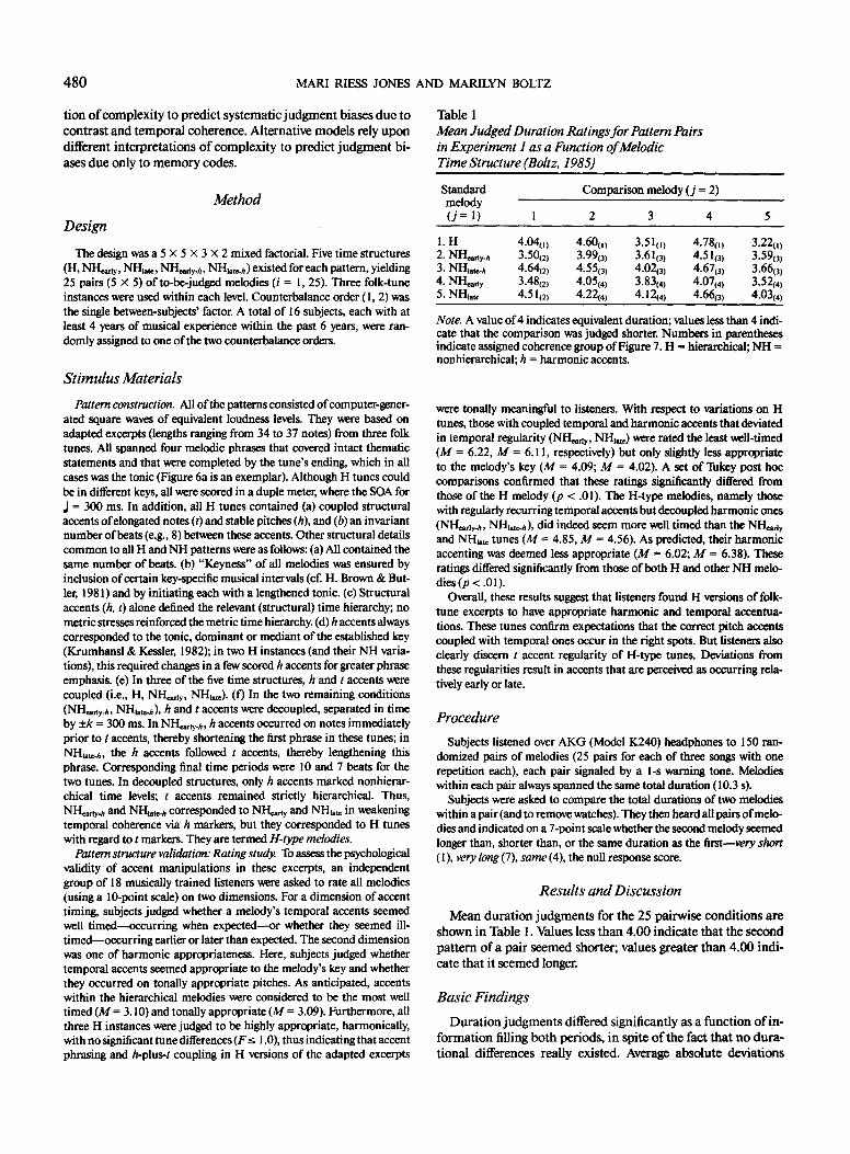
480 MARl RIESS JONES AND MARILYN BOLTZ
tion o f complexity to predict systematic judgment biases due to contrast and temporal coherence. Alternative models rely upon different interpretations o f complexity to predict judgment bi- ases due only to memory codes.
Method
Design
The design was a 5 X 5 X 3 × 2 mixed factorial. Five time structures (H, NHearly, NHl~t~, NI-l~ly.~, NH~te-h) existed for each pattern, yielding 25 pairs (5 × 5) of to-be-judged melodies (i = 1, 25). Three folk-tune instances were used within each level. Counterbalance order (1, 2) was the single between-subjects' factor. A total of 16 subjects, each with at least 4 years of musical experience within the past 6 years, were ran- domly assigned to one of the two counterbalance orders.
Stimulus Materials
Pattern construction. All of the patterns consisted of computer-gener- ated square waves of equivalent loudness levels. They were based on adapted excerpts (lengths ranging from 34 to 37 notes) from three folk tunes. All spanned four melodic phrases that covered intact thematic statements and that were completed by the tune's ending, which in all cases was the tonic (Figure 6a is an exemplar). Although H tunes could be in different keys, all were scored in a duple meter, where the SOA for
= 300 ms. In addition, all H tunes contained (a) coupled structural accents of elongated notes (t) and stable pitches (h), and (b) an invariam number of beats (e.g., 8) between these accents. Other structural details common to all H and NH patterns were as follows: (a) All contained the same number of beats. (b) "Keyness" of all melodies was ensured by inclusion of certain key-specific musical intervals (cf. H. Brown & But- ler, 1981) and by initiating each with a lengthened tonic. (c) Structural accents (h, 0 alone defined the relevant (structural) time hierarchy; no metric stresses reinforced the metric time hierarchy. (d) h accents always corresponded to the tonic, dominant or mediant of the established key (Krumhansl & Kessler, 1982); in two H instances (and their NH varia- tions), this required changes in a few scored h accents for greater phrase emphasis. (e) In three of the five time structures, h and t accents were coupled (i.e., H, NH~riy, NHj~t~). (f) In the two remaining conditions (NH,dy.h, NHl,t~.h), h and t accents were decoupled, separated in time by _+k = 300 ms. In NH,,]y.h, h accents occurred on notes immediately prior to t accents, thereby shortening the first phrase in these tunes; in NHl~t,.h, the h accents followed t accents, thereby lengthening this phrase. Corresponding final time periods were 10 and 7 beats for the two tunes. In decoupled structures, only h accents marked nonhierar- chical time levels; t accents remained strictly hierarchical. Thus, NH~ay.h and NHl,t~.h corresponded to NH~dy and NHl~t~ in weakening temporal coherence via h markers, but they corresponded to H tunes with regard to t markers. They are termed H-type melodies.
Pattern structure validation: Rating study. To assess the psychological validity of accent manipulations in these excerpts, an independent group of 18 musically trained listeners were asked to rate all melodies (using a 10-point scale) on two dimensions. For a dimension of accent timing, subjects judged whether a melody's temporal accents seemed well t i m e d ~ u r r i n g when expected--or whether they seemed ill- timed~oecurring earlier or later than expected. The second dimension was one of harmonic appropriateness. Here, subjects judged whether temporal accents seemed appropriate to the melody's key and whether they occurred on tonally appropriate pitches. As anticipated, accents within the hierarchical melodies were considered to be the most well timed (M = 3.10) and tonally appropriate (M = 3.09). Furthermore, all three H instances were judged to be highly appropriate, harmonically, with no significant tune differences (F < 1.0), thus indicating that accent phrasing and h-plus-t coupling in H versions of the adapted excerpts
Table 1 Mean Judged Duration Ratings for Pattern Pairs in Experiment 1 as a Function of Melodic Time Structure (Boltz, 1985)
Standard Comparison melody ( j = 2) melody ( j r 1) 1 2 3 4 5
1. H 4.04o) 4.60o) 3.51o) 4 . 7 8 o ~ 3.22~) 2. NI-I~ly.h 3 .50(2) 3.99~3~ 3.610) 4.510) 3.590) 3. NHla~h 4.64~2) 4 .55(3 ) 4 .02(3) 4.67o) 3.66(3~ 4. NI"~ y 3.48(2) 4.05(4) 3.83t4 ) 4.07(4) 3.52(4) 5. NHI~ 4.51(2) 4.22t4 ) 4 .12(4 ) 4.66o~ 4.03t4 )
Note. A value of 4 indicates equivalent duration; values less than 4 indi- cate that the comparison was judged shorter. Numbers in parentheses indicate assigned coherence group of Figure 7. H = hierarchical; NH = nonhierarchical; h = harmonic accents.
were tonally meaningful to listeners. With respect to variations on H tunes, those with coupled temporal and harmonic accents that deviated in temporal regularity (NH~ay, NHate) were rated the least well.timed (M = 6.22, M = 6.11, respectively) but only slightly less appropriate to the melody's key (M = 4.09; M = 4.02). A set of Tukey post hoe comparisons confirmed that these ratings significantly differed from those oftbe H melody (p < .01). The H-type melodies, namely those with regularly recurring temporal accents but deeoupled harmonic ones (NI-I~rly.h, NH]a~h), did indeed seem more well timed than the ~ y and NHl,te tunes (M = 4.85, M = 4.56). As predicted, their harmonic accenting was deemed less appropriate (M = 6.02; M = 6.38). These ratings differed significantly from those of both H and other NH melo- dies (p < .01).
Overall, these results suggest that listeners found H versions of folk- tune excerpts to have appropriate harmonic and temporal aecemua- tions. These tunes confirm expectations that the correct pitch accents coupled with temporal ones occur in the right spots. But listeners also clearly discern t accent regularity of H-type tunes. Deviations from these regularities result in accents that are perceived as occurring rela- tively early or late.
Procedure
Subjects listened over AKG (Model K240) headphones to 150 ran- domized pairs of melodies (25 pairs for each of three songs with one repetition each), each pair signaled by a l-s warning tone. Melodies within each pair always spanned the same total duration (10.3 s).
Subjects were asked to compare the total durations of two melodies within a pair (and to remove watches). They then heard all pairs of melo- dies and indicated on a 7-point scale whether the second melody seemed longer than, shorter than, or the same duration as the first--very short ( 1 ), very long (7), same (4), the null response score.
Results and Discussion
Mean durat ion judgments for the 25 pairwise conditions are shown in Table 1. Values less than 4.00 indicate that the second pattern of a pair seemed shorter; values greater than 4.00 indi- cate that it seemed longer.
Basic Findings
Durat ion judgments differed significantly as a function o f in- formation filling both periods, in spite o f the fact that no dura- tional differences really existed. Average absolute deviations

DYNAMIC ATTENDING
Table 2 Predicted and Signed Bias Values (PSEi) of Four Models
481
A PSE~ predictions
Alternative models
Null Chunk Change Melodic pair DM* PSEi DM* PSEi DM* PSEi
Contrast model Observed data A
D~Mi D"Ei PSEi PSEi
Group 1: High coherence
VVI = 0 W, = 0 VV, = 0
H - H 0 0 0 0 0 0 N - NHlate 0 0 + + + + H - NI-l~rly 0 0 + + + + H - NHlat~--h 0 0 + + + + + + H - NH~y. , 0 0 + + + + + +
SDI
W~ =.89
0 0 0 .04 0 -2.67 - .72 - .78 0 2.67 .72 .78 0 -1.33 - .35 - .49 0 2.67 .72 .60
.204 .273
Group 2: Medium coherence
~¢~=0 fv~=0 ~v2=0 NH~t~ - H 0 0 . . . . NI-Ic~y - H 0 0 . . . . N H ~ h - H 0 0 . . . . NH~y.h - H 0 0 . . . .
SD2
~V 2 = .70
0 2.67 .56 .51 0 -2.67 - .56 - .52 0 1.33 .28 .64 0 -2.67 - .56 - .50
.334 .375
Group 3: Medium coherence
~V 3 = 0 W3 = 0 W3 = 0
NHt~h - Nft .ay 0 0 0 0 - - NH|ate-h - NHcaay-h 0 0 0 0 0 0 NHla~h -- NHI~te 0 0 0 0 - - NHlat~.n - NHl~h 0 0 0 0 0 0 NH~arly.h - N H e ~ y 0 0 0 0 -- -- NH~y.h - NH~aay.h 0 0 0 0 0 0 NI '~r ly . h - NI'-Ilate 0 0 0 0 - - NHl~t, - NHearly 0 0 0 0 0 0
SD3
~ t 3 = .40
0 4.00 .48 .67 0 4.00 .48 .55 0 -1.33 - .16 - .34 0 0 0 .02 0 0 0 .51 0 0 0 -.01 0 -5.34 - .64 -.41 0 5.34 .64 .66
.489 .334
Group 4: Low coherence
fv,=o ~v,=o fv,=o NI-I~,ty - N H ~ h 0 0 0 0 + + NI"l~,.h - NHa~h 0 0 0 0 0 0 NOlate - NHlate-h 0 0 0 0 + + NHta~ - NHat~ 0 0 0 0 0 0 NH~ay - NH,~dy.h 0 0 0 0 + + NI"~,ty - NH,~.ty 0 0 0 0 0 0 NHi,tc - NH=dy.h 0 0 0 0 + + NH,.~y - NHh,~ 0 0 0 0 0 0
SD4
'~4 = .22
0 -4.00 - .26 - .17 0 -4.00 - .26 - .39 0 1.33 .08 .12 0 0 0 .03 0 0 0 .05 0 0 0 .07 0 5.34 .35 .22 0 -5.34 - .35 - .48
.422 .373
Note. H = hierarchical; NH = nonhierarchical; h = harmonic accents.
f rom a null difference (4.0) took on a m a x i m u m value o f 0.78, which represents a 22% unidi rec t ional shift on the ra t ing scale. Overall, the in terac t ion o f t ime s t ruc tu re associated wi th the first and second pa t te rns was significant beyond the .0001 level, F(16, 224) = 13.67, MSe = 0.088.
The na tu re o f this in terac t ion suppor t s the Cont ras t Model predict ions. People judged pa t te rns tha t seemed to end " too soon" to be shor t and those tha t seemed to end " l a t e " to be long. Post hoc analyses (Tukey) verified these findings: (a) Type o f cont ras t p roduced significant differences (p < .01 ) between

482 MARI RIESS JONES AND MARILYN BOLTZ
pairs with early versus late endings (e.g., NI-I~a, NHla~). (b) Magnitude of pairwise contrast produced predicted differences in that negligible contrast effects appeared in pairs with equiva- lent single pattern contrasts (e.g., N I - ~ y with NI-~,~y) and in pairs with no contrasts (e.g., H - H). Pairs with nonzero con- trasts, however, yielded systematic differences. (c) Predicted differences as a function of temporal coherence were signifi- cant, with temporal contrast having a greater impact in pairs containing an H melody (p < .01). (d) Effects of contrast were significantly less for pairs containing a melody with decoupled accents (p < .01). (e) Temporal order effects were significant in that a given contrast had more impact whenever an H (p < .01) or H-type (i.e., NHh) melody (p < .05) functioned as a standard. (f) Overall, these findings were robust in generalizing across all three melodic instances (F = 1.0 for melodic instance) and to 12 of the 16 subjects involved (4 subjects tended to show strong contrast effects only in H and not in H-type melodies).
Model Predictions: Contrast Model Versus Alternatives
Several simplifying assumptions are introduced to facilitate predictions about judgment means (from Equations 5-6) and variance (Equation 7) as a function of contrast and temporal coherence.
1. To evaluate the Contrast Model, the linear functionfwith slope a and intercept b = 4 (the null response) relates the re- sponse scale (1-7) to bias predictions of the model. From Equa- tion 6:
PSEi = JD; - 4 = a[WiDEi + (1 - Wi)DM~]. (11)
2. To evaluate the Contrast Model, attending mode parame- ters in Equation 11 are estimated using Equations 8 and 10. The DE~ estimates (Equation 8) are based on the assumption that skilled attenders can use higher order focal periods of musical phrases, an assumption supported by the rating task data re- ported in the Method section. The DMi estimates (Equation 10) are based on the assumption that listeners may alternatively rely on the referent level and count beat periods. This assumption is supported not only by research described earlier (Boltz, 1985; also Footnote 15), but by the present data. That is, under this strategy, DMj = 0, and we show that alternative models based on DM~ ~ 0 are not appropriate for the present task (Table 2). Here, DM~ is weighted by 1 - Wi. This yields the most conser- vative test of the contrast model by reinforcing the true (null) time difference and forcing contrast alone to bias judgments.
3. Each of the 25 melodic pairs was assigned to one of four (k = 1, 2, 3, 4) experimentally designated groups predicted to differ in temporal coherence, as shown in Figure 7. Pairs were categorized according to whether they contained an H or H- type melody and whether this melody was the standard. Thus, event pairs in Groups 1 and 2 have the same absolute amount of contrast but incorporate an H melody either as a standard (Group 1) or as a comparison (Group 2). Similarly, pairs in Groups 3 and 4 involve only NH melodies, in which an H-type pattern is the standard (Group 3) or comparison (Group 4). Interpretations of this parameter lead to the expectation that Wi > V¢2 > ~r3 > ~V4 for VCk- Note that this partitioning has been simplified at the expense of ignoring coherence effects due to marker prominence. For example, Group 1 includes both H - NI-I,ay and H - NI-~r ty . h. If marker prominence is, in fact,
very important, then this particular partitioning may yield poor fits of the Contrast Model.
Predictions of the Contrast Model are summarized in Tables 2 and 3. A priori estimates of DM~ and DE~ are in columns 8 and 9 of Table 2, respectively; the four Wk (above these col- umns) are estimated from the data. Preliminary model fits indi- cated that the common variance of difference scores, o ~, was extremely small, and so it was fixed at zero. Thus, five parame- ters were estimated from the data: four Wk and a scale factor, a. Model fits, using Equation 11, were based on a nonlinear least squares curve-fitting technique (NONLIN), which minimized er- rors between predicted and observed scores, t7 Best-fitting Wk are in Table 2; ~ was .303. This version of the contrast model accounts for 88% of the variance (R2).
Also in Table 2 are predicted and observed values of PSE~ (columns 10 and 11, respectively) and S'Dk (pooled for the kth group) for the Contrast Model, along with predictions of other models. Is Predictions of all models derive from Equation 6. However, those of the Contrast Model are based on nonzero estimates of Wk (and l - Wk), whereas those ofaU other models assume Wk = 0. In terms of Equation 6, when Wk ---- 0, effects of contrast are eliminated and memory effects are maximal [(1 - Wk) = 1.0]. The memory parameter for alternative models is denoted DM*, because it differs conceptually from DM~ of the Contrast Model and also because most models yield only ordinal assessments of memory differences. These are in col- umns 2, 4, and 6. Corresponding directional predictions ofbias (greater or less than) for all melodic pairs are shown in columns 3, 5, and 7 for the Null, Chunk, and Change Models, respec- tively.
A summary of directional (+, - ) prediction accuracy over the four models (of Table 2) appears in Table 3. These indicate that the Contrast Model fares best, predicting 24 of the 25 possi- ble directional differences in time judgments. The Change Model is next with l I of the PSE~s in the correct direction. In other respects, the Contrast Model also proves superior. It cor- re~ly predicts (a) highest temporal coherence for Group l (Wi = .84) and lowest coherence for Group 4 (W4 = .22), (b) maximal temporal contrast effects with least temporal uncer- tainty, namely in Group 1, (c) greater contrast effects for a hier- archical or H-type standard (Groups I and 3) than with an NH standard (Groups 2 and 4) because Wt > W2 and W3 > W4, and (d) least variability in Group 1 in which "~/~ is highest.
The Contrast Model yields a profile that is more accurate and informative than alternatives. However, it does not accommo- date all of the data within this simplified grouping scheme equally well, and its failures are instructive. It describes perfor- mance better in melodic pairs that have clearly marked focal time periods (i.e., in pairs with coupled accents). In fact, when significant model deviations do occur, it is in melodies with de- coupled accents. These patterns present less obvious violations
17 NONLIN (Ohio State Science Package) operates on a least squares algorithm developed by Marquardt (1963), which is basically an inter- polation between Newton-Raphson and gradient methods.
,8 The PSEi predictions of the Contrast Model (column 10) are based on Equation 11 and variance predictions on Equation 7 (with ~ = .303). The D~Mi and D"Et calculations (Table 2, columns 9, 8) axe based on Equations 10 and 8, respectively. See text for DM, ~ calculations of Null, Chunk, and Change Models.

DYNAMIC ATTENDING
FOUR COHERENCE GROUPS
H-type Melody
Standard Comparison
483
Simple H Melody
P r e s e n c e
/ \
A b s e n c e .
GROUP I
I = High Rhythmic Coherence
H - N H
GROUP 5
:5 = Medium Rhythmic Coherence
NHh-NH
GROUP 2
2 = Medium Rhythmic Coherence
NH-H
GROUP 4
4 = Low Rhythmic Coherence
N H - N H h
Figure 7. Four coherence groups of the 25 pairs of melodies used in Experiment 1: Groups 1, 2, 3, and 4.
of expectancies, and so this is not surprising. Although better model fits can be obtained with additional Wk estimates, effects of accentuation are nevertheless clear. We consider this applica- tion of the Contrast Model to be largely illustrative and take these discrepancies to underscore the broader theoretical point that the way in which nontemporal information marks time lev- els is important.
Experiment 2: Productions of Melodic Durations
A second study was designed to confirm that people actually expect patterns to end at particular times. Converging evidence for the psychological reality of expectancies is provided by a production task. A new group oflisteners heard the same melo- dies, without the final three tones, and produced probable end- ing times with a button press. Thus, pure expectancies were made overt via extrapolated productions of the final focal pe- riod.
Some songs, such as NHeady, should encourage anticipations for early endings by virtue of their shorter focal time periods. A~cording to Equation 2, these melodies should lead to shorter final production times. Other songs, such as NH~te, should gen- erate expectancies about late endings and thus yield longer re- sponse times to completion. These predictions derive not from the Contrast Model, but from Equation 2 for timed produc- tions.
Of interest is the reciprocity between produced time and
Table 3 Summary of PSEi Predictions for Four Duration Models
Alternative models No. of Contrast
predictions NuH Chunk Change Model
Total correct 6 10 11 24 Total possible 25 25 25 25
judged time. This involves the prediction that the pattern of produced times will be opposite to the pattern of judged times predicted (and observed) by the Contrast Model. In Experiment 1, for example, NH~tc patterns were predicted to be judged shorter than others, and they were. Here, the claim is if those duration judgments were based on temporal contrasts involv- in_g expectancies, then people will expect these same patterns to last relatively longer and this expectation will be evident in production. The converse, of course, should be true for NHe~y melodies.
Finally, the three alternative models do not predict a recipro- cal pattern of results because none incorporates expectancies. Indeed, memory models taken literally are not particularly con- ducive to extrapolated times because time estimates are based on previously stored information. However, assuming that pro- ductions for a melody are governed by its code complexity, al- ternative models all imply that the pattern of produced times will be similar to judged times for the various H and NH tunes. Thus, either no differences in produced times should arise (Null Model) or NH melodies should yield longer produced times (Chunk and Change Models).
Method
Design
A 5 × 3 × 2 mixed factorial involved crossing the five types of accent/ timing patterns (H, NI-I~y, NH,.~, NI-I~y.h, NHa~.h) with three different songs (used in Experiment 1). Two counterbalance orders formed the single between-subjects factor, 9 subjects, each with at least 4 years of recent musical experience, were assigned to each counterbal- ance order.
Stimulus Materials
Stimulus materials were identical to those of Experiment 1, except that the final three tones were omitted from each melody. Three ran-

484 MARl RIESS JONES AND MARILYN BOLTZ
Table 4 Results of Extrapolation Study (Experiment 2)
Conditions of melodic time structure
Measure H NI-~ly NHearly.h NHlat~ NHlate./~
Mdn extrapolation time (in ms) 1154 899 1173 1209 1305
Mdn accuracy score (in ms) -46 -301 -27 +309 + 105
Mno. ofjudged missing beats 2.67 1.59 2.56 3.11 3.24
Note. Entries in each row reflect, respectively, one of three dependent measures used in Experiment 2 to indicate expectancies about musical endings for five melodic conditions. Median extrapolation time for missing notes (row 1) and its accuracy (row 2; negative sign indicates anticipation) are given along with the mean number of beats judged missing (row 3). H = hierarchical; NH = nonhierarchical; h = harmonic accents.
domized blocks, each with 15 melodies, occurred within two counter- balance orders.
Procedure
Subjects performed two tasks. The first involved extrapolations; the second required judgments of the number of missing notes.
Production. Recorded instructions told subjects to (a) listen to in- complete melodies whose final (1 to 5) notes, including the closing tonic, were missing, and (b) indicate when a melody should end if miss- in_g notes were played in real time. Four practice trials clarified the pro- cedure.
On each trial, a 1-s warning tone (5000 hz) preceded a melody by 2 s. When the last note of a melody was signaled by a panel light, sub- jects covertly continued the tune and indicated its true ending time by a button press. This extinguished the signal light, and the next trial be- gan. This phase lasted 40 min.
Judgments of missing tones. Recorded instructions told subjects to judge, in writing, how many notes were missing from each melody. Sub- jects then heard the same 15 experimental melodies, now randomized according to one of two schedules. On each of 15 trials, a 5000-hz warn- ing tone preceded the melody by 2 s; after the melody, subjects had 5 s to respond.
Results and Discussion
Table 4 presents the results in which averages are based on data collapsed over melodic instance and counterbalance order, both of which again produced negligible effects (F < 1.00). Overall, the findings are remarkably congruent with those in- volving judged durations.
Average median extrapolation times for each melodic type are in the first row of Table 4. Mean differences were significant, F(4, 64) = 7.48, MSe = 54,724.97, p < .0001, and reflect expec- tancies about early and late endings. Longest times were those predicted to generate expectancies for late endings (NHlate, NHlate-h), and the shortest times occurred for NI-Iearly tunes. Al- though NHlate was significantly longer than NH~arly (p < .01, Schefl~), this was not true of NHl~te-h versus NI-I~r~y.h (. 10 < p < .05), although differences here were in the predicted direction. Accuracy scores (in ms) appear in the second row of Table 4 and reflect temporal discrepancies between produced and observed endings. They should correspond to estimates of temporal con- trast if people had actually heard the melody continue. Note
that pairs in which phrases were prominently marked by cou- pled structural accents, NH~r~y versus NHlate, yield greater differences than ones with less prominent (i.e., decoupled ac- cents) markings, NHeady-h versus NHlate-h. People are relatively accurate in predicting endings of hierarchical melodies, and they are also accurate with NI~ay_h melodies. One reason for this may be that in those NH melodies with decoupled accents, temporal accentuation remains hierarchical. If people ignore harmonically marked phrasings and rely solely on t accents, then these NH melodies can indeed function as H-type time structures. At least in some cases, people did this.
Finally, the average number of missing beats reported by lis- teners (row 3, Table 4) converges with time measures. In all im- portant respects, statistical analysis here confirms that similar profile differences exist and these generalize across the majority of subjects used in this study.
Overall, these data favor an interpretation that moderately skilled listeners detect and use temporal relationships to gener- ate expectancies about musical endings. More recent work rely- ing on different melodies and task requirements confirms these results (Van Vreden, Boltz, & Jones, 1989). Together, such find- ings reinforce the assumption that temporal contrast arises from expectancy violations. The pattern of over- and underesti- mated final periods, which is opposite to the pattern of duration judgments (Experiment 1), supports the idea that temporal contrast is based on listeners' extrapolations (temporal expec- tancies).
General Discussion
Together, Experiments 1 and 2 suggest that duration judg- ments and overt productions of musical events reflect a com- mon activity. Related conclusions have been drawn by others using different stimulus materials (Keele, Pokorny, Corcos, & Ivry, 1985; Kristofferson, 1984). Our explanation centers on the role of expectancies in extrapolations and in selective attune- ments in duration judgments. Equation 2, which describes ex- trapolations, and Equations 5-6, which describe judgments, to- gether predict the observed pattern of reciprocal outcomes over the two tasks.
A primary aim of Experiments 1 and 2 was to approximate a natural context in which future-oriented attending would ap-
DYNAMIC ATTENDING 485
pear. Folk tunes, particularly coherent ones, fit the stimulus re- quirements. Reliance on moderately skilled musical listeners further ensured a possibility of future-oriented attending and simplified estimation of DE~. Although both constraints limit experimental generality, they succeeded in demonstrating the existence of future-oriented attending. These findings suggest that when skilled attenders interact with relatively coherent time patterns, temporal expectancies will arise and duration judgments can be biased by temporal contrast. Related influ- ences of temporal contrast have been reported in other contexts as well (Kidd, in press; Kristofferson, 1977; Lehiste, 1975, 1977).
The present results are difficult to explain in terms of con- temporary models that emphasize memory for accumulated amounts of nontemporal information. For example, in Experi- ment 1 the Null Model predicts that all melodies should be judged equal in duration because the number of tones and pitch changes are identical. And yet some were judged longer (i.e., NH~,ly, NH~rly-h) and others shorter (i.e., NHt~t~, NHlate-h). Differences in number of chunks or in changing accent patterns (Chunk, Change Models) also cannot account for these effects. Although melodies of a pair can differ in relative timing of cer- tain accents, even models addressed to rhythmic chunking have difficulties because they fail to acknowledge that accent patterns incite dynamic and preparatory attending.
The Contrast Model weights the influence of contrast so that over- or underestimates of durations due to contrast are most evident in coherent events in which future-oriented attending occurs more often. It turns out that in event pairs with low tem- poral coherence (e.g., some NH-NH pairs), estimates of tempo- ral contrast could be quite high. Yet, according to this model, these DE`. values should not have proportional impact on judg- ments, and they do not. According to the Contrast Model, ex- pectancies are less likely and analytic attending with beat- counting strategies are more likely in judging these tunes. As a result, tendencies to correctly judge two events as identical in total duration are reinforced. Of course, in other cases, if events differ in number of beat periods, then tendencies to over- or underestimate duration will emerge (see Boltz, 1985). Thus, both attending modes may have been used in the present stud- ies, a possibility supported by the fact that greater variability also appears in judgments involving pairs with moderate to low coherence.
Finally, although the overall emphasis here has been on DE~, in principle the DM~ parameter lends itself to several interpre- tations. As with DE,-, this parameter can reflect the way some- one uses time at any of several different levels (e.g., chunks or groups of beats). That is, people will not always rely on beat counting; they may analytically attend over other levels, levels that correspond to things other than beats. Part 1 indicates that amount of information (defined in various ways) does seem to bias time judgments in certain contexts. The present study and the Contrast Model suggest some reasons for these seemingly conflicting findings on the filled duration effect: The way infor- mation fills an interval to mark different time levels and the way a person attends to this information can affect time estimates.
In short, memory-oriented approaches to duration judgment must be supplemented, and the Contrast Model illustrates one way to do this. It incorporates some version of a memory-based model through the concept of analytic attending. It does so by
expressing the idea that effortful memory activities and expec- tancies are stimulated by different contexts, ones at opposite ends of the structural coherence continuum.
Summary of Part 4
A reciprocal pattern of findings emerged from two experi- ments involving comparative duration judgments (Experiment 1) and timed productions (Experiment 2) in which attending mode and temporal coherence were varied. Experiment 1 find- ings support the Contrast Model's proposition that duration judgments are a function of weighting attending mode parame- ters (temporal contrast, mnemonic differences) by degree of co- herence. Experiment 2 findings suggest that contrast itself de- pends on temporal expectancies about musical endings.
Part 5: Conclusions
In this article we derived illustrative models of time judgment and production from a general theoretical framework in which both attending mode and event coherence figure. These models have some potential for explaining ways in which rhythmical attenders who use relative time nonetheless estimate intervals of time in different tasks. They also address divergent findings surrounding the filled interval effect. In Part 5, we conclude with general observations about the theoretical framework that relate to issues of generality, biological bases of attending, and philosophical views of time.
Theoretical Generality." Is a Rhythmic Approach Warranted?
The assumption of inherent rhythmicity in both the environ- ment and the attender is a basic one. Because its claim to gener- ality can be questioned, let us be clear about what it does and does not mean. It means that temporal patterning exists in envi- ronmental energy patterns and in the structure of attending over time. It does not mean that these patternings are immediately obvious, necessarily simple, or rigidly fixed. Indeed, the main point of our earlier discussion of environmental structure was to illustrate that formalization of time structure is a challenging goal, one demanding careful identification of functional time markers, marker couplings/strength, and various time transfor- mations. The very success of another, quite different approach to rhythmicity, fourier analysis, should discourage ideas that in- herent periodicities of events and attending activities can be su- perficially discerned.
At the level of the Contrast Model, the relative impact of sim- pie and complex rhythmicities is expressed through attentional weights that assume a continuum of dynamic environmental complexity. It posits conditions in which evidence of simple rhythmicities will appear, and clearly these are not ubiquitous. Temporally incoherent events do exist. Our claim is simply that ready attunements to such complex events will fail in particular and sometimes meaningful (e.g., contrast) ways, given the na- ture of rhythmic attending. In this sense, the approach has greater generality than those time estimation models cited in Part 1 that focus largely on events with low temporal coherence. Interestingly, it achieves this by reconceiving the elusive con-

486 MARI RIESS JONES AND MARILYN BOLTZ
struct of complexity in rhythmic terms and suggesting a range of dynamic complexity based on temporal coherence.
There is no doubt that people are often forced to judge the duration of complex events with arbitrary time spans. The way this might occur has been illustrated in Parts 3 and 4 using mu- sical events. Perhaps the Contrast Model will not generalize to comparable, nonmusical situations involving skilled attenders. Although this restriction remains a possibility, we think some formalization of constructs such as expectancy, contrast, and analytic attending will be useful for future models. Ultimately, the value of a fundamental assumption is found in its poten- tial for stimulating explanations of diverse psychological phenomena.
Biological Clocks Versus a Rhythmic Attending Perspective
Oearly, the basic assumptions about inherent rhythmicity, when considered with respect to the attender, imply a biological foundation for attunements. The bias toward a biological un- derstanding is shared by others who provide additional support for the inherent rhythmicity of animate beings (e.g., Kelso et al., 1985).
With regard to theories of time estimation, however, biologi- cally based theories have become unfashionable. Ornstein (1969) was most explicit in pointing to limitations of biological chronometers: "Although psychologis ts . . , have attempted to study time experience there has been a maze of postulated pos- sible mechanisms proposed for time. One major r e a s o n . . . [is t h a t ] . . , time has been treated a s . . . sensory process" (p. 34).
Ornstein (1969) correctly criticized earlier approaches for their disagreement on a specific time base. However, his alterna- tive storage size hypothesis rests on equally confusing guidelines concerning complexity, ones that do not reliably predict time judgments. Nevertheless, because our approach envisions a bio- logical basis, it is useful to distinguish the way time is conceived here from the way it is viewed in models of a strict biological clock.
Strictly speaking, a clock is a timekeeper that abstracts an absolute interval from the time dimension to serve as a fixed interval time base. Its appeal in time estimation often involves arousal effects that are handily accommodated by assuming that the interval time base shortens or lengthens with, for exam- ple, drugs or boredom. Nevertheless, as a biological metric the clock concept reinforces the idea that time is independent of the structure of particular events because the clock interval indis- criminately measures both arbitrary and nonarbitrary time pe- riods. For example, a 5-rain interval is arbitrary when defined only by clock numbers, but not when it coincides with the be- ginning and end of a bird's song a child's game, or a conversa- tion. Yet such distinctions are irrelevant for a clock model that exclusively counts elapsed time. Furthermore, the choice of a single time interval as a clock itself is a problem, as Ornstein (1969) noted. For a clock model to be sensitive to nested time periods, there must be postulates referring to clocks within clocks, as well as a master clock that somehow controls and monitors their interactions. Finally, each clock must be intelli- gent: it must "know" how to identify its salient markers, those that correspond to meaningful beginnings and ends of its partic- ular intervals. Most psychological versions of clock models be-
gin as simple ones that do not directly reflect either relative time (e.g., time ratios, time contrasts) or structural markings. Conse- quently, they become complicated and unparsimonious when explanations of special goal-directed temporal sensitivities are required. For example, the roles of expectancy violations and temporal contrast as well as those of flexible and/or effortful attending remain difficult to incorporate into clock models. In- stead, clock models encourage a search for a central timing mechanism (master clock) that monitors absolute intervals and for psychological time limits that are interval in nature. These are dubious undertakings in light of current data (e.g., Jones, 1976; Kolers & Brewster, 1985; van Noorden, 1971) and the arguments supplied here on the relational nature of timing and temporal limits (e.g., dominance region; see Footnote 12).
In our view, the biological basis for responses to event time takes the form of attunement rhythms that selectively entrain, that shift over nested levels, and eventually are shaped by the event itself. Attending is based directly on relative time, and this results in temporal flexibility in which neither the referent time base nor focal attending levels are rigidly fixed. Thus, various arousal effects can also be addressed within this theory via refer- ent level shifts. But the major advantage of the current approach over strict clock models is found in its predictions concerning focal attendings relative to some referent level. For instance, ex- pectancies and temporal contrast derive directly from analyses of dynamic interactions of an attender with patternings of envi- ronmental structure. In effect, the structure of a temporally co- herent event can function as a natural timekeeper for the at- tender. Instead of a clock-timed world, the attender responds to a dynamic event-timed world in which time judgments depend on an event's characteristic timing and on how its structure con- firms or disconfirms some expected course. Of course, this sort of attending is less likely with incoherent events. In this case people may resort to analytic attending or an even more practi- cal strategy: They may check their watches. In fact, we predict that people will refer to external timekeepers more frequently in relatively unstructured situations.
In proposing that dynamic events afford different, biologi- cally based attentional perspectives (e.g., future-oriented vs. an- alytic), we also raise other issues with regard to attending. Our experimental focus has been on time estimation, but the con- ceptual framework has broader implications, ones that distin- guish it from other approaches to attention that are less con- cerned with attending over time. As a consequence, this ap- proach has greater applicability to patterns of speech, music, dance, and so on, in which the concept of attunement levels may be fruitful (Jones, 1986). It introduces the possibility that people rely directly on event structure to achieve different tem- poral perspectives for different goals. These perspectives can re- sult in different estimates of relative duration in time estima- tion. Dynamic complexity enters in to qualify how one uses event structure to achieve the requisite perspective. But in other situations and goals, attending perspectives and complexity may yield alternative models. Furthermore, by linking different at- tentional perspectives to distinctive time levels within each event, this approach avoids the homunculus problem that also troubles certain attentional theories (see Johnston & Dark, 1986). Finally then, this approach incorporates responsiveness to goals and event functions that is not evident in other models of attention and memory, including those adapted to time esti-
DYNAMIC ATTENDING 487
mation that were mentioned in Part 1. In sum, the construct of attending levels suggests a way in which environmental infor- mation can selectively control attending in time and also afford potential referent levels from which other aspects of the envi- ronment can be attended.
S o m e Philosophical Implicat ions
Finally, some of our distinctions inevitably invite comparison with Bergson's (1944, 1950) notion of "lived" time versus "measured" time. In reacting to Kant 's (1900) claim that time is an internal intuition that allows separations of object repre- sentations on an infinite time line (i.e., "in relations of time"; Kant, 1900, pp. 28-31 ), Bergson (1950) argued that
Kant's great mistake was to view time as a homogeneous medium. He did not notice that real duration is made up of moments inside one another, and that when it seems to assume the form of a homo- geneous whole, it is because it gets expressed in space. (p. 232)
For Bergson, nonhomogeneity characterizes experienced time because things experienced first always affect (interpenetrate) things experienced subsequently in time; this irreversibility de- scribes time intervals as we live through them. It is not captured by the expression of a time line (Jones, 1987b).
Clearly, our concepts of temporal nesting, attunements, ex- pectancy, and contrast capture some Bergsonian aspects of lived time. But Bergson and Kant present essentially phenomenologi- cal approaches in that both assume that only privately experi- enced time is real, because the time of external objects is con- structed. And for both, this phenomenal time is essentially in- terval in character, and operates in an absolute fashion (see, e.g., Bergson's, 1965, reply to Einstein). By contrast, ours is not a phenomenological account. Nor do we conceive of time inter- vals in absolute terms. We assume that both the environment and its organisms exhibit temporal patternings that are recipro- cally related and shared during attending activities. The inter- nal time structure ofattunements and expectancies is inextrica- bly tied to the external time structure of transformationally re- lated event changes. In order to interact, both must exist.
References
Abel, S. (1972a). Discrimination of temporal gaps. Journal of the Acous- tical Society of America, 52, 519-524.
Abel, S. (1972b). Duration discrimination of noise and tone bursts. Journal of the Acoustical Society of America, 51, 1219-1223.
Adams, R. (1977). Intervening stimulus effects of category judgments of duration. Perception and Psychophysics, 21, 527-534.
Allan, L. ( i 979). The perception of time. Perception and Psychophysics, 26, 340-354.
Apel, W. (1972). Harvard dictionary of music (2nd ed). Cambridge, MA: Balknap Press of Harvard University Press.
Avant, L., & Lyman, P. (1975). Stimulus familarity modifies l~rceived duration in prerecognition visual processing. Journal of Experimen- tal Psychology: Human Perception and Performance, 1, 205-213.
Baker, C. H. (1962). On temporal extrapolation. Canadian Journal of Psychology 16, 37--41.
Barclay, C. D., Cutting, J. E., & Kozlowski, L. T (1978). Temporal and spatial factors in gait perception that influence gender recognition. Perception and Psychophysics, 23, 145-152.
Bartlett, N. R., & Bartlett, S. C. (1959). Synchronization of a motor
response with an anticipated sensory event. PsychologicalRevie~, 66, 203-218.
Benjamin, W. E. (1984). A theory of musical meter. Music Perception, 1, 355--413.
Bergson, H. (1944). Creative evolution (A. Mitchell, Trans.). Toronto: Random House, Canada Limited.
Bergson, H. (1950). Time and freewill (E L. Pogson, Trans.). London: George Allen & Unwin.
Bergson, H. (1965). Duration and simultaneity (L. Jacobson, Trans.). New York: Bobbs-Merrill.
Berry, W. (1976). Structural functions in music. Englewood Cliffs, NJ: Prentice Hall.
Block, R. (1974). Memory and the experience of duration in retrospect. Memory and Cognition, 2, 153-160.
Block, R. (1978). Remembered duration: Effects of event sequence complexity. Memory and Cognition, 6, 320-326.
Block, R. (1985). Contextual coding in memory: Studies of remem- bered duration. In J. Michon & J. Jackson-Roy (Eds.), Time, mind, andbehavior(pp. 169-178). Heidelberg, FRG: Springer-Vcrlag.
Block, R. (in press). Experiencing and remembering time: Affordances, context, and cognition. In I. Levin & D. Zakay (Eds.), Timeandhu- man cognition: A life-span perspective. Amsterdam: North Holland.
Block, R., George, E. J., & Reed, M. A. (1980). A watched pot some- times boils: A study of duration experience. Acta Psychologica, 46, 81-94.
Block, R., & Reed, M. (1978). Remembered duration: Evidence for a contextual-change hypothesis. Journal of Experimental Psychology: Human Learning and Memo~ 4, 656-665.
Bolinger, D. L. (1958). A theory of pitch accent. Word, 14, 109-149. Boltz, M. (1985). An expectancy model of judged duration: An ecologi-
cal perspective. Unpublished doctoral dissertation, Ohio State Uni- versity Library.
Boltz, M., & Jones, M. R. (1986). Does rule recursion make melodies easier to reproduce? If not, what does? Cognitive Psychology,, 18, 389- 431.
Brown, H. (1988). The interplay of set content and temporal context in a functional theory of tonality perception. Music Perception, 5, 219- 250.
Brown, H., & Butler, D. (1981). Diatonic trichord as minimal tonal cue- cells. In Theory Only, 5, 39-55.
Brown, S. W. (1985). Time perception and attention: The effects of pro- s0ective versus retros0ective paradigms and task demands on per- ceived duration. Perception and Psychophysics, 38, 115-124.
Burnside, W. ( 1971). Judgment of short time intervals while performing mathematical tasks. Perception and Psychophysics, 9, 404 ~06.
Butler, D., & Brown, H. (1984). Tonal structure versus function: Studies of the recognition of harmonic motion. Music Perception, 2, 6-24.
Carlsoo, S. (1972). How man moves. (W. P. Michael, Trans.). New York: Distributed by Cran, Russak, & Co.
Clarke, E. E (1984). Structure and expression in the rhythm of piano performance. Unpublished doctoral dissertation, University of Exe- ter, Exeter, Devon, England.
Clarke, E. E (1985a). Some aspects of rhythm and expressions in Ixn'for- manees of Erik Satie's "Gnossienne No. 5." Music Perception, 2, 299-328.
Clarke, E. E (1985b). Structure and expression in rhythmic perfor- mance. In P. Howell, I. Cross, & R. West (Eds.), Musical structure and cognition (pp. 209-236). London: Academic Press.
Clynes, M. (1978). Sentics: The touch of emotions. Garden City, NJ: Anchor Press.
Coxeter, H. S. M., & Greitzer, S. L. (1967). Geometry revisited. New York: Random House.
Condon, W. S., & Sander, L. W. (1974). Synchrony demonstrated be- tween movements of the neonate and adult speech. Child Develop- ment, 45. 456--462.

488 MAR1 RIESS JONES AND MARILYN BOLTZ
Cone, E. (1968). Musical form and musical performance. New York: Norton.
Craik, R., & Lockhart, R. (1972). Levels of processing: A framework for memory research. Journal of Verbal Learning and Verbal Behav- ior, 11,671-684.
Cutler, A., & Isard, S. D. (1980). The production of prosody. In B. But- terworth (Ed.), Language production: Vol. 1. Speech and talk (pp. 245-269). New York: Academic Press.
Cutting, J. (1982). Two ecological perspectives: Gibson vs. Shaw and Turvey. American Journal of Psychology,, 95, 199-222.
Dentsch, D., & Feroc, J. (1981). The internal representation of pitch sequences in tonal music. Psychological Review, 18, 503-522.
Devane, J. (1974). Word characteristics and judged duration for two response sequences. Perception and Motor Skills, 38, 525-526.
Divenyi, P., & Danner, W. (1977). Discrimination of time intervals marked by brief acoustic pulses of various intensities and spectra. Perception and Psychophysics, 21, 125-142.
Divenyi, P., & Sachs, (1978). Discrimination of time intervals bounded by tone bursts. Perception and Psychophysics, 24, 429-436.
Dowling, W. J., & Harwood, D. L. (1985). Music cognition. New York: Academic Press.
Essens, E J. (1986). Hierarchical organization of temporal patterns. Perception and Psychophysics, 40, 69-73.
Essens, E J., & Povel, D. J. (1985). Metrical and nonmetrical represen- tations of temporal patterns. Perception andPsychophysics, 37, 1-7.
Fowler, C. (1983). Converging sources of evidence on spoken and per- ceived rhythms of speech: Cyclic production of vowels in monosyl- labic stress feet. Journal of Experimental Psychology: General, 112, 386-412.
Fraisse, E (1956). Les structures rhythmiques [Rhythmic structures]. Louvain, France: Editions Universitaires.
Fraisse, E (1964). The psychology of time. London: Eyre & Spotti- woode.
Fraisse, E (1982). Rhythm and tempo. In D. Deutsch (Ed.), The psy- chology of music (pp. 149-180). New York: Academic Press.
Fraisse, E (1984). Perception and estimation of time. Annual Review of Psychology, 35, 1-36.
Frankenhauser, M. (1959). Estimation of time: An experimental study. Stockholm, Sweden: Almquist & WikseU.
Freyd, J. J. (1987). Dynamic mental representations. PsychologicaIRe- view, 94, 427-438.
Fry, D. B. (1958). Experiments in the perception of stress. Language andSpeech, 1, 126-152.
Gabrielsson, A. ( 1974). Performance of rhythm patterns. Scandinavian Journal of Psychology, 15, 63-74.
Gabrielsson, A. (1985). Interplay between analysis and synthesis in studies of music performance and music experience. Music Percep- tion, 3, 59-68.
Gabrielsson, A., Bengtsson, I., & Gabrielsson, B. (1983). Performance of musical rhythm in 3/4 and 6/8 meter. Scandinavian Journal of Psychology, 24, 193-213.
Gentner, D. R. (1987). Timing of skilled motor performance: Tests of the proportional duration model. Psychological Review, 94, 255-276.
Getty, D. (1975). Discrimination of short temporal intervals: A com- parison of two models. Perception and Psychophysics, 18, 1-8.
Getty, D. (1976). Counting processes in human timing. Perception and Psychophysics, 20, 191-197.
Gibson, J. J. (1966). The senses considered as perceptual systems. Bos- ton: Houghton Mifflin.
Gibson, J. J. (1979). The ecological approach to visual perception. Bos- ton: Houghton Mifflin.
Gray, J. (1968). Animal locomotion. New York: Norton. Hahn, J., & Jones, M. R. (1981). Invariants in auditory frequency.
Scandinavian Journal of Psychology, 92, 627-651. Halpern, A., & Darwin, L. (1982). Duration discrimination in a series
of rhythmic events. Perception andPsychophysics, 31, 86-89.
Hamilton, E, & Hockey, R. (1974). Active selection of items to be re- membered. Cognitive Psychology, 6, 61-83.
Handel, S. (1984). Using polyrhythms to study rhythm. Music Percep- tion, I, 465-484.
Handel, S., & Oshinsky, J. S. (1981). The meter of syncopated auditory polyrhythms. Perception and Psychophysics, 30, 1-9.
Hicks, R., Miller, G., & Kinsborne, M. (1976). Prospective and retro- spective judgments of time as a function of amount of information processed. American Journal of Psychology, 89, 719-730.
Hirsh, I. J., Bilger, R. C., & Deatherage, B. H. (1969). The effect of auditory and visual background on apparent duration. American Journal of Psychology, 69, 561-574.
Hogan, H. (1975). Time perception and stimulus preference as a func- tion of stimulus complexity. Journal of Personality and Social Psy- chology, 31, 32-35.
Inman, V. T (1966). Human locomotion. Canadian Medical Associa- tion Journal, 94, 1047-1054.
Jackson, J. L. (1985). Is the processing of temporal information auto- matic or controlled? In J. A. Michon & J. L. Jackson (Eds.), Time, mind and behavior (pp. 179-190). Berlin: Springer-Verlag.
Jagacinski, R., Marshburn, E., Klapp, S. T., & Jones, M. R. (1988). Tests of parallel versus integrated structure in polyrhythmic tapping. Journal of Motor Behavior, 20, 416-442.
Johansson, G. (1973). Visual perception of biological motion and a model for its analysis. Perception and Psychophysics, 14, 201-211.
Johansson, G. (1975). Visual motor perception. Scientific American, 232, 76-89.
Johnson, W. W. (1986). Studies in motion extrapolation. Unpublished doctoral dissertation, Ohio State University, Columbus.
Johnston, W. A., & Dark, V. J. (1986). Selective attention. In M. R. Rosenzweig & L. W. Porter (Eds.), Annual review of psychology (Vol. 37, pp. 43-75). Palo Alto, CA: Annual Reviews.
Jones, M. R. (1976). Time, our lost dimension: Toward a new theory of perception, attention, and memory. Psychological Review, 83, 323- 335.
Jones, M. R. (198 l a). Only time can tell: On the topology of mental space and time. Critical Inquiry, 7, 557-576.
Jones, M. R. (1981b). A tutorial on some issues and methods in serial pattgTn research. Perception and Psychophysics, 30, 492-504.
Jones, M. R. (1981c). Music as a stimulus for psychological motion: Part 1. Some determinants of expectancies. Psychomusicology,, 1, 34- 51.
Jones, M. R. (1982). Music as a stimulus for psychological motion: Part 2. An expectancy model. Psychomusicology, 2, 1-13.
Jones, M. R. (1985). Structural organization of events in time: A review. In J. A. Michon & J. L. Jackson (Eds.), Time, mind, and behavior (pp. 192-214). Heidelbergo FRG: Springer-Verlag.
Jones, M. R. (1986). Attentional rhythmicity in human perception. In J. R. Evans & M. Clynes (Eds.), Rhythm in psychological, linguistic, and music processes (pp. 13-40). Springfield, IL: Charles C Thomas.
Jones, M. R. (1987a). Perspectives on musical time. In A. Gabrielsson (Ed.), Action and perception in rhythm and music (pp. 153-175). Stockholm, Sweden: Royal Swedish Academy of Music.
Jones, M. R. (1987b). Some thoughts on the relevance of Bergson to contemporary psychology. In A. C. Papanicolaou & P. A. Y. Gunter (Eds.). Bergson and modern thought: Towards a unified science (pp. 250-270). New York: Harwood Academic Publishers.
Jones, M. R., & Boltz, M., & Kidd, G. (1982). Controlled attending as a function of melodic and temporal context. Perception and Psycho- physics, 32, 211-218.
Jones, M. R., Kidd, G., & Wetzel, R. (1981). Evidence for rhythmic attention. Journal of Experimental Psychology: Human Perception and Performance, 7, 1059-1073.
Kant, I. (1900). Critique of pure reason. (J. M. D. Meiklejohn, Trans.). New York: Colonial Press.
Keele, S. W., & Hawkins, H. (1982). Explorations of individual differ-

DYNAMIC ATTENDING 489
ences relevant to high level skill. Journal of Motor Behavior, 14, 3- 23.
Keele, S. W., Pokorny, R. A., Corcos, D. M., & Ivry, R. (1985). Do perception and motor perception share common timing mechanisms: A correlation analysis. Acta Psychologica, 60, 173-191.
Kclso, J. A. S., Holt, K. G., Rubin, P., & Kugler, P. (1981). Patterns of human interlimb coordination emerg~ from the properties of non- linear, limit cycle oscillatory processes: Theory and data. Journal of Motor Behavior, 13, 226-261.
Kidd, G. (1984). The perception of tonal relationships in music. Unpub- lished doctoral dissertation, The Ohio State University Library.
Kidd, G. (in press). Articulatory-rate context effects in phoneme identi- fication. Journal of Experimental Psychology: Human Perception and Performance.
Klapp, S. T. (1979). Doing two things at once: The role of temporal compatibility. Memory and Cognition, 7, 375-381.
Klapp, S. T. (1981). Temporal compatibility in dual motor tasks: II. Simultaneous articulation and hand movement. Memory and Cogni- tion, 9, 398-401.
Klapp, S. T., Hill, M., Tyler, J., Martin, Z., Jagacinski, R., & Jones, M. R. (1985). On marching to two different drummers: Perceptual aspects of the difficulties. Journal of Experimental Psychology: Hu- man Perception and Performance, 11, 814--827.
Kolata, G. (1985). Finding biological echos in fetuses. Science, 230, 929-930.
Kolers, P. A., & Brewster, J. M. (1985). Rhythms and responses. Journal of Experimental Psychology: Human Perception and Performance, 11, 150-167.
Kozhevnikov, V., & Chistovich, L. (1965). Speech: Articulation andper- ception (Rep. No. JPRS 30543). Washington, DC: Joint Publications Research Service.
Kramer, J. (1982). Beginnings and endings in Western art music. Cana- dian University Music Review,, 3, 1-14.
Kristoffetson, A. B. (1976). Low-variance stimulus-response latencies: Deterministic interval delays? Perception and Psychophysics, 20, 89- 100.
Kristofferson, A. B. (1977). A real-time criterion theory of duration discrimination. Perception and Psychophysics, 21, 105-117.
Kristofferson, A. B. (1980). A quantal step function in duration dis- crimination. Perception and Psychophysics, 27, 300-306.
Kxistofferson, A. B. (1984). Quantal and deterministic timing in human duration discrimination. Annals of the New York Academy of Sci- ences, 423, 3-15.
Kronman, U., & Sundberg, J. (1987). Isthe musical ritard an allusion to physical motion? In A. Gabrielsson (Ed.), Action and perception in rhythm and music (pp. 57-68). Stockholm, Sweden: Royal Swedish Academy of Music.
Krumhansl, C. L. (1979). The psychological representation of musical pitch in a tonal content. Cognitive Psychology, 11, 346-374.
Krumhansl, C. L., & Kessler, E. J. (1982). Tracing the dynamic changes in perceived tonal organization in a spatial representation of musical keys. Psychological Review,, 89, 334--368.
Ladd, D. R. (1986). Intonational phrasing: The case for recursive pro- sodic structure. Phonology Yearbook, 3, 311-340.
Laws, K. (1985). Physics and dance. American Scientist, 73, 426--432. Lee, C. S. (1985). The rhythmic interpretation of simple musical se-
quences: Towards a perceptual model. In P. Howell, I. Cross, & R. West (Eds.), Musical structure and cognition (pp. 53-69). London, Academic Press.
Lee, D. N. (1980). The optic flow field: The foundation of vision. Philo- sophical Transactions of the Royal Society of London, 290, 169-179.
Leeuwenbew, E. (1969). Quantitative specification of information in sequential patterns. PsychologicalReview, 76, 216-220.
Lehiste, I. (1975, August). The perception of duration within sequences offour intervals. Paper presented at the 8th International Congress of Phonetic Sciences, Leeds, England.
Lehiste, I. (1976). Suprasegmental features of speech. In N. J. Lass (Ed.), Contemporary issues in experimental phonetics (pp. 225-239). New York: Academic Press.
Lehiste, I. (1977). Isochrony revisited. Journal of Phonetics, 5, 253- 263.
Lerdahl, E, & Jackendoff, R. (1983). A generative theory of tonal music. Cambridge, MA: MIT Press.
Liberman, M., & Prince, A. (1977). On stress and linguistic rhythm. Linguistic lnqui~ 8, 249-336.
Longuet-Higgins, H. C., & Lee, C. S. (1982). The perception of musical rhythms. Perception, I1, 115-128.
Longuet-Higgius, H. C., & Lee, C. S. (1984). The rhythmic interpreta- tion of monophonic music. Music Perception, 1, 424-441.
Marquardt, D. W. (1963). An algorithm for least-squares estimation of nonlinear parameters. SIAM Journal of Applied Mathematics, 11, 431--441.
Martin, J. 0972). Rhythmic (hierarchical) versus serial structure in speech and other behavior. Psychological Review, 79, 487-509.
Mas~ D. J. (1983). Perceiving and counting sounds: The roles of pitch distance, rhythm and grouping. Unpublished doctoral dissertation, Ohio State University.
Michon, J. A., & Jackson, J. L. (1985). The psychology of time. In J. A. Michon, & J. L. Jackson (Eds.), Time, mind, and behavior (pp. 2- 17). Heidelberg, FRG: Springer-Verlag.
Monahan, C. B., & Carterette, E. C. (1985). Pitch and duration as deter- minants of musical space. Music Perception, 3, 1-32.
Navon, D., & Gopher, D. (1979). On the economy of the human pro- cessing system. Psychological Review, 86, 214--255.
Neisser, U., & Becklen, R. (1975). Selective looking,: Attending to visu- ally specified events. Cognitive Psychology,, 7, 480-494.
Newtson, D., Hairfield, J., Bloomingdale, J., & Cutino, S. (1987). The structure of action and interaction. Social Cognition, 5, 191-237.
Ornstein, R. (1969). On the experience of time. Baltimore, MD: Pen- guin Books.
Paccia-Cooper, J., & Cooper, W. E. (1981). The processing of phrase structures in speech production. In E D. Eimas & J. L. Miller (Eds.), Perspectives on the study of speech (pp. 311-336). Hillsdale, NJ: Erl- baum.
Penner, M. (1976). The effect of marker variability on the discrimina- tion of temporal intervals. Perception and Psychophysics, 19, 466- 469.
Pickett, J. M. (1980). The sounds of speech communication. Baltimore, MD: University Park Press.
Pierson, K. (1976). Control of walking. Scientific American, 235, 72- 86.
Pike, K. (1945). The intonation of American English. Ann Arbor: Uni- versity of Michigan Press.
Piston, W. (1978). Harmony (4th ed., revised and expanded by Mark De Voto). New York: Norton.
Povel, D. J. (1977). Temporal structure of performed music: Some pre- liminary observations. Acta Psychologica, 41, 309-320.
Povel, D. J. (1981). Internal representations of simple temporal pat- terns. Journal of Experimental Psychology: Human Perception and Performance, 7, 3-18.
Povel, D. J., & Essens, P. (1985). Perception of temporal patterns. Music Perception, 2, 411--440.
Poynter, W. ( 1983). Duration judgment and the segmentation of experi- ence. Memory and Cognition, I I, 77-82.
Poynter, W., & Homa, D. (1983). Duration judgment and the experi- ence of change. Perception and Psychophysics, 33, 548-560.
Reber, A. S., Kassin, S. M., Lewis, S., & Cantor, G. (1980). On the rela- tionship between implicit and explicit modes in the learning of a com- plex rule structure. Journal of Experimental Psychology: Human Learning and Memo~ 5, 492-502.
Seherer, K. (1979). Acoustic concomitants of emotional dimensions: Judging affect from synthesized tone sequences. In S. Weitz (Ed.),
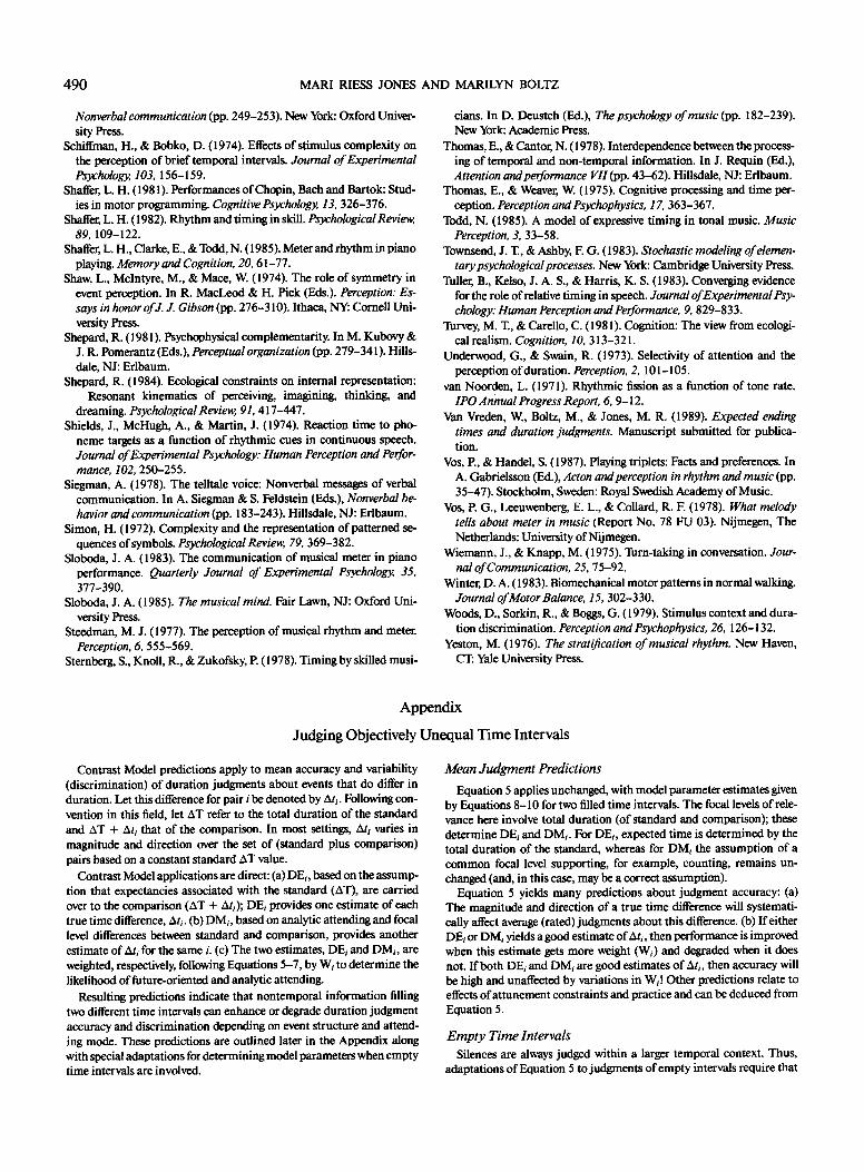
490 MARI RIESS JONES AND MARILYN BOLTZ
Nonverbal communication (pp. 249-253). New York: Oxford Univer- sity Press.
Schiffman, H., & Bobko, D. (1974). Effects of stimulus complexity on the perception of brief temporal intervals. Journal of Experimental Psychology, 103, 156-159.
Shaffer, L. H. (1981). Performances of Chopin, Bach and Bartok: Stud- ies in motor programming. Cognitive Psychology,, 13, 326-376.
Shaffer, L. H. (1982). Rhythm and timing in skill. PsychologicaIReview, 89, 109-122.
Shaffer, L. H., Clarke, E., & Todd, N. (1985). Meter and rhythm in piano playing. Memory and Cognition, 20, 61-77.
Shaw, L., McIntyre, M., & Mace, W. (1974). The role of symmetry in event perception. In R. MacLeod & H. Pick (Eds.). Perception: Es- says in honor of J. J. Gibson (pp. 276-310). Ithaca, NY: Cornell Uni- versity Press.
Shepard, R. (1981). Psychophysical complementarity. In M. Kubovy & J. R. Pomerantz (Eds.), Perceptual organization (pp. 279-341 ). Hills- dale, NJ: Erlbanm.
Shepard, R. (1984). Ecological constraints on internal representation: Resonant kinematics of perceiving, imagining, thinking~ and
dreaming. Psychological Review, 91, 417-447. Shields, J., McHugh, A., & Martin, J. (1974). Reaction time to pho-
neme targets as a function of rhythmic cues in continuous speech. Journal of Experimental Psychology: Human Perception and Perfor- mance, 102, 250-255.
Siegrnan, A. (1978). The telltale voice: Nonverbal messages of verbal communication. In A. Siegman & S. Feldstein (Eds.), Nonverbal be- havior and communication (pp. i 83-243). HiUsdale, NJ: Erlbaum.
Simon, H. (1972). Complexity and the representation of patterned se- quences of symbols. Psychological Review, 79, 369-382.
Sloboda, J. A. (1983). The communication of musical meter in piano performance. Quarterly Journal of Experimental Psychology,, 35, 377-390.
Sloboda, J. A. (1985). The musical mind. Fair Lawn, NJ: Oxford Uni- versity Press.
Steedman, M. J. (1977). The perception of musical rhythm and meter. Perception, 6, 555-569.
Sternberg, S., Knoll, R., & Zukofsky, P. (1978). Timing by skilled musi-
cians. In D. Deustch (Ed.), The psychology of music (pp. 182-239). New York: Academic Press.
Thomas, E., & Cantor, N. (1978). Interdependence between the process- ing of temporal and non-temporal information. In J. Requin (Ed.), Attention and performance VII (pp. 43-62). Hillsdale, N J: Erlbaum.
Thomas, E., & Weaver, W. (1975). Cognitive processing and time per- ception. Perception and Psychophysics, 17, 363-367.
Todd, N. (1985). A model of expressive timing in tonal music. Music Perception, 3, 33-58.
Townsend, J. T., & Ashby, E G. (1983). Stochastic modeling ofelemen- tart psychological processes. New York: Cambridge University Press.
Tuller, B., Kelso, J. A. S., & Harris, K. S. (1983). Converging evidence for the role of relative timing in speech. Journal of Experimental Psy- chology: Human Perception and Performance, 9, 829-833.
Turvey, M. T., & Carello, C. (1981). Cognition: The view from ecologi- cal realism. Cognition, 10, 313-32 I.
Underwood, G., & Swain, R. (1973). Selectivity of attention and the perception of duration. Perception, 2, 101-105.
van Noorden, L. (1971). Rhythmic fission as a function of tone rate. IPO Annual Progress Report, 6, 9-12.
Van Vreden, W., Boltz, M., & Jones, M. R. (1989). Expected ending times and duration judgments. Manuscript submitted for publica- tion.
Vos, P., & Handel, S. (1987). Playing triplets: Facts and preferences. In A. Gabrielsson (Ed.), Acton and perception in rhythm and music (pp. 35-47). Stockholm, Sweden: Royal Swedish Academy of Music.
"Cos, P. G., Leeuwenberg, E. L., & Collard, R. E (1978). What melody tells about meter in music (Report No. 78 FU 03). Nijmegen, The Netherlands: University of Nijmegen.
Wiemann, J., & Knapp, M. (1975). Turn-taking in conversation. Jour- nal of Communication, 25, 75-92.
Winter, D. A. ( 1983). Biomechanical motor patterns in normal walking. Journal of Motor Balance, 15, 302-330.
Woods, D., Sorkin, R., & Boggs, G. (1979). Stimulus context and dura- tion discrimination. Perception and Psychophysics, 26, 126-i 32.
Yeston, M. (1976). The stratification of musical rhythm. New Haven, CT." Yale University Press.
A p p e n d i x
J u d g i n g O b j e c t i v e l y U n e q u a l T i m e I n t e r v a l s
Contrast Model predictions apply to mean accuracy and variability (discrimination) of duration judgments about events that do differ in duration. Let this difference for pair i be denoted by At1. Following con- vention in this field, let AT refer to the total duration of the standard and AT + Ah that of the comparison. In most settings, At,- varies in magnitude and direction over the set of (standard plus comparison) pairs based on a constant standard AT value.
Contrast Model applications are direct: (a) DE~, based on the assump- tion that expectancies associated with the standard (AT), are carried over to the comparison (AT + At/); DE~ provides one estimate of each true time difference, Ah. (b) DMi, based on analytic attending and focal level differences between standard and comparison, provides another estimate of Ati for the same i. (c) The two estimates, DEi and DMi, are weighted, respectively, following Equations 5-7, by W~ to determine the likelihood of future-oriented and analytic attending.
Resulting predictions indicate that nontemporal information filling two different time intervals can enhance or degrade duration judgment accuracy and discrimination depending on event structure and attend- ing mode. These predictions are outlined later in the Appendix along with special adaptations for determining model parameters when empty time intervals are involved.
Mean Judgment Predictions
Equation 5 applies unchanged, with model parameter estimates given by Equations 8-10 for two filled time intervals. The focal levels of rele- vance here involve total duration (of standard and comparison); these determine DEi and DMj. For DE. expected time is determined by the total duration of the standard, whereas for DM~ the assumption of a common focal level supporting, for example, counting, remains un- changed (and, in this case, may be a correct assumption).
Equation 5 yields many predictions about judgment accuracy: (a) The magnitude and direction of a true time difference will systemati- cally affect average (rated) judgments about this difference. (b) If either DEi or DM/yields a good estimate of At. then performance is improved when this estimate gets more weight (W`.) and degraded when it does not. If both DE/and DM/are good estimates of At,, then accuracy will be high and unaffected by variations in W~! Other predictions relate to effects ofattunement constraints and practice and can be deduced from Equation 5.
Empty Time Intervals Silences are always judged within a larger temporal context. Thus,
adaptations of Equation 5 to judgments of empty intervals require that

DYNAMIC ATTENDING 491
(a) the temporal coherence parameter reflects the context provided by the succession of interval markers, for example, in a surrounding phrase (prose, musical) or in an experimental session (psyehophysical setting), (b) DEj remains tied to expectancies about total event durations, whereas DM~ reflects differences due to counting, tapping, and other temporally based activities in which a person engages and uses to subdi- vide some empty time period, and (c) the referent level is determined by the most frequent, prominently marked time contextual period. Given this, predictions about empty interval judgments follow from Equations 5-6. As before, these suggest that attending mode and tempo- ral context should affect judgment accuracy and bias.
The role of temporal contrast in the latter predictions is reminiscent of Kxistofferson's (1977, 1984) real time criterion in his modeling of duration judgments of empty intervals. However, there are significant differences. One is that the real-time criterion model addresses only speeded responding in two choice judgment tasks (long and short). That task encourages and the model depicts responding only to the relative temporal order of expected versus observed ending times. The Contrast Model applies to comparative time interval estimates of expected versus observed ending times. A second is that neither attending modes and temporal coherence are found in the real-time criterion model. A di- chotomous attending model has also been presented by Thomas and Cantor (1978) for empty and filled intervals. However, it applies only to durations less than 100 ms, and although the model does consider effects due to different amounts of information, it cannot address contrast effects arising from temporal expectancies. Conceptually, its parameters differ.
Variance and Time Discrimination Predictions
When Equation 7 (variance prediction) involves DE~ and DM; pa- rameters, both of which estimate the difference in total time of the two intervals (i.e., Ati), it can be used to make predictions about time-dis- crimination performance in a classic psychophysieal context. That is, if Ati values about some AT are small, temporal threshold issues arise. Conventionally, time discrimination thresholds (JNDs) are estimated from the standard deviation of observed judgments over the event pairs (i) associated with a given standard interval, AT, namely SD(AT). A critical design constraint is that the At~ values form a balanced set for each AT, so that their sum (over standard/comparison pairs) is zero. Thus, to adapt Equation 7 to express SD(AT), parameters DEi, DMi, and W~ must be averaged over appropriate event pairs i having a com- mon AT Taking the square root:
JND = SD(AT) = [a2[W(1 - WXDE - DM) 2 + 02]]1/2. (A1)
In this form, diseriminability is a function of temporal coherence (W), attentional estimates (DE, DM) of the average At~ value (i.e., At = 0), and an average base error variance, o-2 (for either filled and empty intervals given previous assumptions). Thus, the discriminability func- tion relating JND to AT can take different forms, with some at variance with Weber's Law for time discrimination. Equation AI also predicts that nontemporal information filling two different intervals can affect their discriminability. Both predictions must be justified.
Weber's Law holds that a temporal JND is a constant proportion of AT. It is supported if SD(AT) is a constant proportion of AT for all AT, implying a linear relation between JND and AT. Weber's Law is not compatible with Equation A 1 because it does not predict discriminabil- ity to vary as a function ofattending mode, coherence, context, practice, and so on. Nonetheless, Equation A 1 is worth exploring, given that little empirical support exists for a simple version of Weber's Law (e.~, Allan, 1979; Divenyi & Danner, 1977; Getty, 1976; Halpern & Darwin, 1982; Kristofferson, 1976; Povel, 1977). Although temporal discriminability is good over a range of time intervals (50-2,000 ms), JNDs are not linear functions of AT as predicted by Weber's Law. In fact, the diseriminabil- ity function varies with different factors. Two illustrative cases deal re- spectively with skilled and unskilled attending.
Skilled attending and JND invariance with A T. Threshold invariance is predicted by Equation AI if(DE - DM) 2 = 0. This occurs if people reliably estimate the true time differences, Ati, regardless of attending mode. That is, because DE~ and DMi each estimate Ati values, their sums (over i), like those of Ati values themselves, will be zero if all are good estimates. Because skilled attending is flexible attending, either of the two attending modes may be used to arrive at the correct Ati esti- mates. If DE = DM = 0, Equation AI becomes
SD(AT) = (a202) '/2. (A2)
The 02 is the (average) variance of difference distributions and with skilled observers its constancy is reasonable. Therefore, a202 = Vr, a variance component that is independent of stimulus durations (Getty, 1975).
Some predictions are as follows: (a) Asymptotically, thresholds are invariant with AT. (b) Given a fixed (modal) referent period, dominance region constraints imply range limits to predicted threshold invariance (i.e., invariance obtains only within limiting AT values, with JNDs in- creasing monotonically with larger AT values, ones outside the domi- nance region range). (c) Variations in temporal coherence do not affect asymptotic performance (i.e., W[I - W] vanishes!). Although some support exists for these first two predictions (Kristofferson, 1980, 1984), no evaluations exist for the third prediction.
Unskilled attending and monotonically increasing JNDs. Following Equation A1, a monotonic function occurs if the term (DE - DM) 2 0 and increases with AT This is predicted with unskilled judges and/or a wide range of AT values (see attunement constraints, Part 2). In such cases, regardless of attending mode, unreliable estimates of At~ occur, leading to nonzero average estimates of both DE and DM (see mean judgments). In general, (DE - DM) 2 should increase with AT because (a) [At/[ increases proportionately with AT, and (b) dominance region constraints imply that disparities between expected and observed times will increase as the latter exceed the dominance region.
Finally, Equation A1 leads to Getty's (1975) generalized version of Weber's Law, ifW and 02 are invariant with changes in AT Thus, if AT are constrained in range and without systematic sequential patterning within a session, then we assume k 2 = W(I - W) and Vr = a202. When- ever a2(DE - DM) 2 approximates AT 2, then Equation A 1 yields
SD(AT) = [k2(AT 2 -I- V r ) ] 1/2. (A3)
Predictions regarding skill level and AT range have some support (Kristofferson, 1980, 1984). With respect to temporal coherence (W), at least with discriminations of empty intervals, the relative timing of markers of differential prominence within an experimental session (context) significantly affects performance (e.g~, Abel, 1972a, 1972b; Divenyi & Sachs, 1978; Penner, 1976). In sum, the predicted discrimi- nability function takes different forms depending on the way Contrast Model parameters reflect attending skill, task constraints, instructions, and context.
Nontemporal Information
Within two different intervals, nontemporal information can affect discriminability according to Equation A 1. Although this prediction creates apparent problems for the Contrast Model because effects of nontemporal information on judgments about equal time intervals have not been reliably reported for time discriminations (Allan, 1979; Woods, Sorkin, & Boggs, 1979), it is resolved in Equations A1-A2. These equations predict that such effects do not always occur and more- over, that when nontemporal information does affect threshold perfor- mance, it will either enhance or degrade performance depending upon attending mode.
Received May 31, 1988 Revision received October 11, 1988
Accepted October 25, 1988 •