Dynamic Behavior of Mode Partition Noise in MMF

Petar PepeljugoskiIBM Research

1

Motivation and Issues• Inconsistent treatment of mode partition noise (MPN) and relative intensity noise (RIN) in spreadsheet model– Need for ISI correction  

• Original MPN theory SD formula is:– calculated at the center of the bit interval (assumes does not change over the bit interval)

– applicable to single mode fibers (SMF) only, no bit pattern and launch conditions dependence

• How to apply to multimode fibers (MMF)• Are current inputs backed by measurements?

– k‐factor currently used may be wrong– are all lasers the same (i.e. number of modes, spacing between modes, rms linewidth)

2

0 50 100 150 200 250 300 350 400 450-8

-6

-4

-2

0

2

4

6

8

What is MPN• laser modes fluctuate in synchronism ‐

overall signal noise is small (noise in laser modes anti‐correlated)

• It can be a major source of noise in links with MULTIMODE lasers and large chromatic dispersion 

• propagation in dispersive media destroys mode "synchronization" ‐large mode fluctuations can be destructively combined at the receiver ‐this extra noise is called mode partition noise (MPN)

Time (distance)

Wavelength

0 100 200 300 400 500 600 700 800 900 1000-5

-4

-3

-2

-1

0

1

2

3

4

5

Blue ‐ Laser OutputGreen ‐ Long Fiber Output

Noise in individual modes at LD Output Combined Noise (all modes) at RX output

Approach• Start with the theory developed by Ogawa and Agrawal [1,2]

– Major assumption is that the mode partition noise is calculated in the center of the eye – this is what the spreadsheet model does

• Calculate the MPN SD at each point in the bit interval– Use Gaussian approximation for the laser spectrum; also check with 

measured spectrums– Use this result later for MMF

• Compare the SM result with the exact calculation over the entire bit interval– Accuracy check point: the results should be the same at the center of 

the eye (confirmed)– Do not normalize the SD

• Extend calculations to multimode fibers and arbitrary bit patterns– Use mode power distributions (MPD) and mode group delays (MGD) in 

the calculation– Extend the approach to arbitrary bit pattern

4

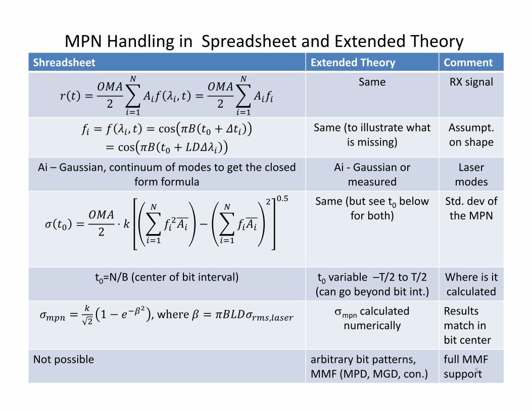
MPN Handling in  Spreadsheet and Extended TheoryShreadsheet Extended Theory Comment

2 , 2

Same RX signal

, coscos

Same (to illustrate what is missing)

Assumpt.on shape

Ai – Gaussian, continuum of modes to get the closed form formula

Ai ‐ Gaussian or measured

Laser modes

2 ⋅

. Same (but see t0 below for both)

Std. dev of the MPN

t0=N/B (center of bit interval) t0 variable –T/2 to T/2(can go beyond bit int.)

Where is it calculated

1 , where , mpn calculatednumerically

Results match in bit center

Not possible arbitrary bit patterns, MMF (MPD, MGD, con.) 

full MMF support5

MPD SD calculation over the entire bit interval• Make same assumptions as Ogawa and Agrawal [1,2]

– only one fiber mode propagates– cosine shape for received signal, Gaussian laser spectrum

• Set L = 0.1km, k = 0.3, = 850nm, BitRate = 25Gb/s, same rmslinewidth as measured spectrum (numbers for illustration purposes)

• Calculation repeated for measured laser spectrum (measurement on 30 Gb/s laser)

-0.5 -0.4 -0.3 -0.2 -0.1 0 0.1 0.2 0.3 0.4 0.50

0.01

0.02

0.03

0.04

0.05

0.06

0.07

0.08

Decision time offset [u.i.]

Nor

mal

ized

M

PN [

a.u.

]

Gaussian spectrum, exactSpreadsheet modelMeasured spectrum, exact

Accuracy check: SM and exact calculation agree at eye center 6

® IEEE 2012

MPN SD calculation (cont’d)

• Calculations of SD using the spreadsheet model and exact calculation agree at the center of the eye for one propagating fiber mode – Implication is the calculations are correct

• Figure shows the MPN SD increases away from the center of the eye– Both measured spectrum and Gaussian approximation for the spectrum have the same shape, with small difference in SD magnitude and possible time offset

– Important for MMF, since mode group delays will introduce additional delays

7

Extension to MMF

Signal in each mode group,

Overall signal at fiber output

Overall standard deviation at the fiber output

Easily found following Ogawa and Agrawal’sformalism [1,2]

1 1

,2

M N

i jj i

ij iOMA

y t MPD f t t A

8

Extension to MMF• Get a fiber MPD and normalized MGD, use measured 

spectrum• Calculate the standard deviation for each mode group 

(use the results for one mode fiber, properly weigh the results using MPDs)

0 2 4 6 8 10 12 14 16 180

0.05

0.1

0.15

Mode group Number

Nor

mal

ized

Mod

e P

ower

0 2 4 6 8 10 12 14 16 180

0.05

0.1

0.15

0.2

0.25

0.3

Mode group Number

Mod

e G

roup

Del

ay [n

s/km

]

MPD into the fiber Fiber Mode Group Delays  9

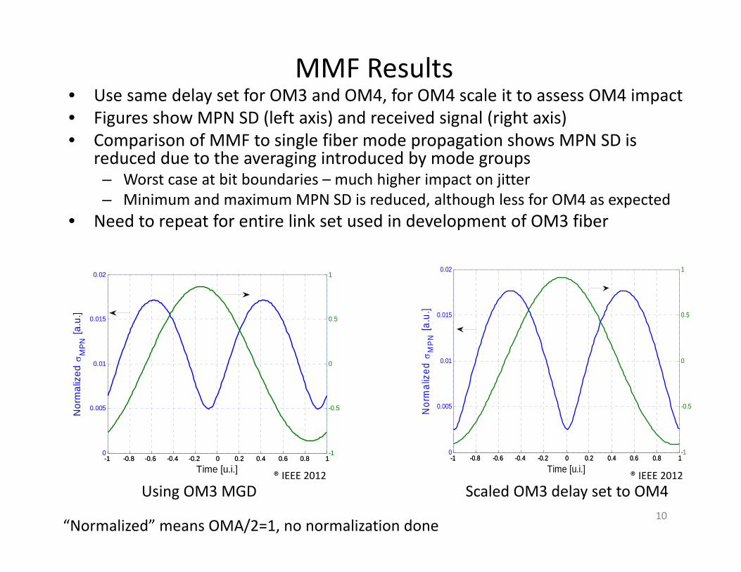
MMF Results• Use same delay set for OM3 and OM4, for OM4 scale it to assess OM4 impact• Figures show MPN SD (left axis) and received signal (right axis)• Comparison of MMF to single fiber mode propagation shows MPN SD is 

reduced due to the averaging introduced by mode groups– Worst case at bit boundaries – much higher impact on jitter– Minimum and maximum MPN SD is reduced, although less for OM4 as expected

• Need to repeat for entire link set used in development of OM3 fiber

-1 -0.8 -0.6 -0.4 -0.2 0 0.2 0.4 0.6 0.8 10

0.005

0.01

0.015

0.02

Time [u.i.]

Nor

mal

ized

M

PN [

a.u.

]

-1 -0.8 -0.6 -0.4 -0.2 0 0.2 0.4 0.6 0.8 1-1

-0.5

0

0.5

1

-1 -0.8 -0.6 -0.4 -0.2 0 0.2 0.4 0.6 0.8 10

0.005

0.01

0.015

0.02

Time [u.i.]

Nor

mal

ized

M

PN [

a.u.

]

-1 -0.8 -0.6 -0.4 -0.2 0 0.2 0.4 0.6 0.8 1-1

-0.5

0

0.5

1

Using OM3 MGD Scaled OM3 delay set to OM4

“Normalized” means OMA/2=1, no normalization done10

® IEEE 2012 ® IEEE 2012

MPD SD for Data Pattern – One Fiber Mode

• ISI does not impact the minimum value of the MPN SD• MPN SD depends on the slope of the signal 

0 2 4 6 8 10 12 14 16 180

0.02

0.04

0.06

Time [bit intervals]0 2 4 6 8 10 12 14 16 18

0

0.02

0.04

0.06

Time [bit intervals]

Nor

mal

ized

M

PN [

a.u.

]

0 2 4 6 8 10 12 14 16 18-1

0

1

2

Sig

nal A

mpl

itude

[a.u

.]

11

MPN SD for All Mode Groups• Calculations repeated for all mode groups

– MPN SD does not become smaller for higher ISI points– Minimum MPN SD value becomes larger– MPN SD depends on the slope of the signal – the larger the slope the 

higher the MPN SD

0 2 4 6 8 10 12 14 160

0.005

0.01

0.015

Time [bit intervals]

Nor

mal

ized

M

PN [

a.u.

]

0 2 4 6 8 10 12 14 16-1

0

1

2

Sig

nal A

mpl

itude

[a.u

.]

ISI at fiber output = 1.9 dB 12® IEEE 2012

MPN SD for All Mode Groups• Bits with higher ISI have higher MPN SD

– Need correction in Spreadsheet Model

Bit 6 has higher ISI than bit 4 or bit 1

0 2 4 6 8 10 12 14 160

0.005

0.01

0.015

Time [bit intervals]

Nor

mal

ized

M

PN [

a.u.

]

0 2 4 6 8 10 12 14 16-1

0

1

2

Sig

nal A

mpl

itude

[a.u

.]

Yet, MPN SD lowest for bit 1, highest for bit 6

13

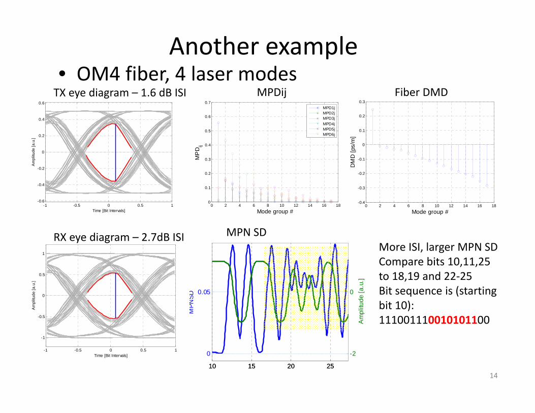
Another example• OM4 fiber, 4 laser modes 

14

-1 -0.5 0 0.5 1-0.6

-0.4

-0.2

0

0.2

0.4

0.6

Time [Bit Intervals]

Am

plitu

de [a

.u.]

0 2 4 6 8 10 12 14 16 180

0.1

0.2

0.3

0.4

0.5

0.6

0.7

Mode group #

MP

Dij

MPD1jMPD2jMPD3jMPD4jMPD5jMPD6j

0 2 4 6 8 10 12 14 16 18-0.4

-0.3

-0.2

-0.1

0

0.1

0.2

0.3

Mode group #

DM

D [p

s/m

]

TX eye diagram – 1.6 dB ISI MPDij Fiber DMD

-1 -0.5 0 0.5 1

-1

-0.5

0

0.5

1

Time [Bit Intervals]

Am

plitu

de [a

.u.]

RX eye diagram – 2.7dB ISI

10 15 20 25

0

0.05

MPN

SD

10 15 20 25

-2

0

Am

plitu

de [a

.u.]

More ISI, larger MPN SDCompare bits 10,11,25 to 18,19 and 22‐25Bit sequence is (starting bit 10):111001110010101100

MPN SD

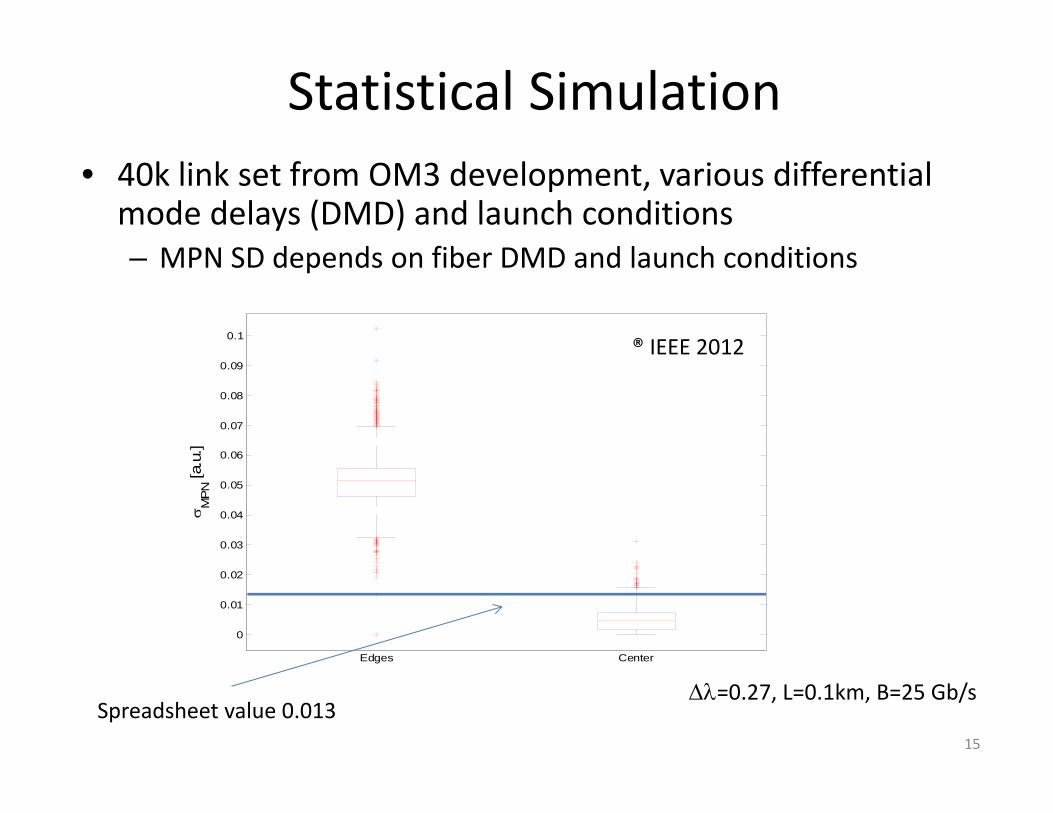
Statistical Simulation• 40k link set from OM3 development, various differential mode delays (DMD) and launch conditions– MPN SD depends on fiber DMD and launch conditions

0

0.01

0.02

0.03

0.04

0.05

0.06

0.07

0.08

0.09

0.1

Edges Center

M

PN [a

.u.]

Spreadsheet value 0.013=0.27, L=0.1km, B=25 Gb/s

15

® IEEE 2012

Conclusion• Extended MPN theory developed by Ogawa and Agrawal to 

explore:– MPN SD over the entire bit interval– dependence of MPN SD on launch conditions and fiber DMD in 

MMF– MPN SD with arbitrary pattern with or without ISI

• Two mechanisms working in opposite direction, need to assess the overall effect– MPN SD increases away from the bit center– MMF introduces averaging effect, lowering MPN SD

• MPN SD currently calculated by the spreadsheet not suitable to assess the impact on the jitter– MPN SD at bit boundaries may be quite high– High ISI values will increase the effect of MPN SD

16

We Need Correction for ISI in The Spreadsheet Model

• Need to divide MPN SD by ISI in the spreadsheet model– Lower ISI does not mean higher MPN SD

• Multiple consecutive 1’s or 0’s have very little or no MPN SD

• MPN SD statistically lower than what the SM predicts– How to include that in the SM

• Further investigate MPN, request more scrutiny in power/jitter budget presentations

17

References[1]. Agrawal, Antony and Shen: "Dispersion Penalty for 1.3 um LightwaveSystems with Multimode Semiconductor Lasers", IEEE Journal of LightwaveTechnology, Vol. 6 No.5, 1988, pages 620‐625[2] Ogawa: "Analysis of Mode Partition Noise in Laser Transmission Systems", IEEE Journal of Quantum Electronics, Vol. QE‐18, No. 5, May 1982, pages 849‐855[3] Pepeljugoski, P.: “Dynamic Behavior of Mode Partition Noise in Multimode Fiber Links”, IEEE Journal of Lightwave Technology, Vol. 30, No.15, August 2012, pp. 2514‐2519.

18

Backup Slides

19

Signal Eye diagrams

• ISI at laser output is ~1.52 dB• ISI at the fiber output is ~1.9 dB

0 0.1 0.2 0.3 0.4 0.5 0.6 0.7 0.8 0.9 1-1.5

-1

-0.5

0

0.5

1

1.5

Time [bit intervals]

Am

plitu

de [

a.u.

]

0 0.1 0.2 0.3 0.4 0.5 0.6 0.7 0.8 0.9 1-1.5

-1

-0.5

0

0.5

1

1.5

Time [bit intervals]

Am

plitu

de [

a.u.

]

20

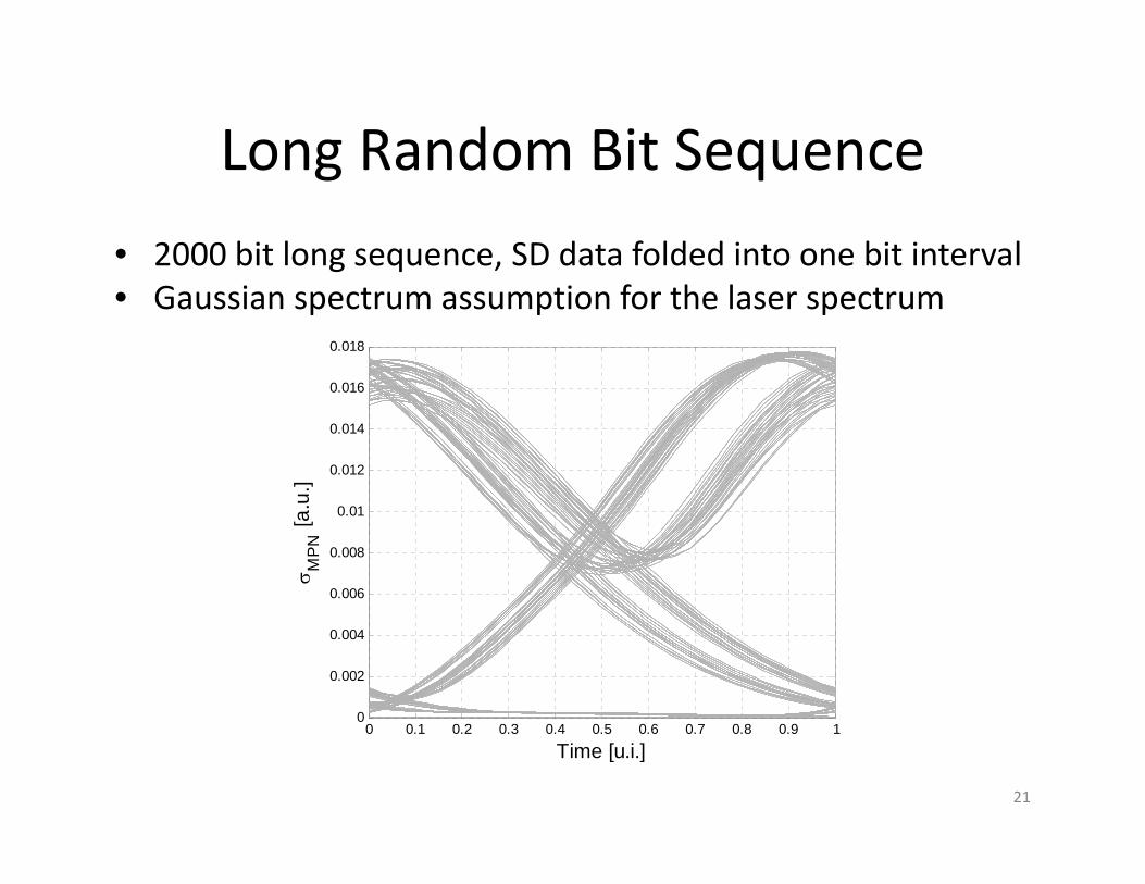
Long Random Bit Sequence• 2000 bit long sequence, SD data folded into one bit interval• Gaussian spectrum assumption for the laser spectrum

0 0.1 0.2 0.3 0.4 0.5 0.6 0.7 0.8 0.9 10

0.002

0.004

0.006

0.008

0.01

0.012

0.014

0.016

0.018

Time [u.i.]

MPN

[a.

u.]

21

Two fibers, two launch conditionssame bandwidth – very different eyesa b

22

Signal shape is important in MPN –>  launch conditions, DMD lead to variability