dynamic composition of functionalities of networked ... · entific research documents, whether they...
TRANSCRIPT

HAL Id: tel-00436707https://tel.archives-ouvertes.fr/tel-00436707v2
Submitted on 27 Nov 2009
HAL is a multi-disciplinary open accessarchive for the deposit and dissemination of sci-entific research documents, whether they are pub-lished or not. The documents may come fromteaching and research institutions in France orabroad, or from public or private research centers.
L’archive ouverte pluridisciplinaire HAL, estdestinée au dépôt et à la diffusion de documentsscientifiques de niveau recherche, publiés ou non,émanant des établissements d’enseignement et derecherche français ou étrangers, des laboratoirespublics ou privés.
Dynamic Composition of Functionalities of NetworkedDevices in the Semantic Web
Sattisvar Tandabany
To cite this version:Sattisvar Tandabany. Dynamic Composition of Functionalities of Networked Devices in the Seman-tic Web. Computer Science [cs]. Université Joseph-Fourier - Grenoble I, 2009. English. <tel-00436707v2>

UNIVERSITE JOSEPH FOURIER – GRENOBLE 1
Ecole Doctorale Mathematiques, Sciences et Technologies de l’Information, Informatique
Dynamic Composition of
Functionalities of Networked Devices
in the Semantic Web
THESE
presentee et soutenue publiquement le 23 novembre 2009
pour l’obtention du
Doctorat de l’Universite Joseph Fourier – Grenoble 1
(specialite informatique)
par
Sattisvar TANDABANY
Directeur de these : Marie-Christine ROUSSET
Composition du jury
President : Christine COLLET Professeur ENSIMAG Grenoble INP – Grenoble
Rapporteurs : Djamal BENSLIMANE Professeur a l’UCBL – LyonFarouk TOUMANI Professeur a l’Universite du Sud – Toulon
Directeur de these : Marie-Christine ROUSSET Professeur a l’UJF – Grenoble
Laboratoire d’Informatique de Grenoble

.

The gift given without any hope for reward, with a sense ofduty, is given in proper place and time to a deserving person,that gift is said to be pure.
Bhagavad-Gita, XVII
Acknowledgment
The path taken by this thesis was not predictable in its beginning. The tortuous meanders it has mademe follow have uncovered significant people to interact with. I wish to express in these few lines mygratitude to all those people with whom I was able to complete this thesis.
In particular, I extend my sincere thanks to my supervisor Professor Marie-Christine Rousset, whoguided me throughout these years of my PhD, who committed to this adventure, who has undeniablymanaged to show me that the light at the end of this tunnel was not the headlight of another locomotive.What the research means to me and how much I am attached to it is thanks to her.
I feel particular deference to Professor Yuzuru Tanaka who welcomed me for one year in his labor-atory in Sapporo, Japan. I owe him for sharpening my scientific cultivation through lengthy discussions.With him I learned the proverb that framed my concept of time:
“Nothing is more precious than time, so there is no greater generosity than to waste it withoutcounting”
I also thank Professors Djamal Benslimane and Farouk Toumani, for their careful reading of thismanuscript and their report, and Professor Christine Collet for chairing the jury of my PhD.
My research was enhanced by teaching, and this activity let me explore a different facet of research:pedagogy. I thank therefore Michel Burlet and Jean-Pierre Peyrin for their invaluable advice regardingthe transmission of knowledge.
My work took place primarily within the team HADAS at Grenoble. I thank its members for theirhelp and support through the last days. I think especially of my fellow office and other doctoral studentswho shared with me moments of distraction: Remi, Benjamin, Noha, Charlotte, Christine, Diana, andNaga.
My stays in Japan made me mingle with people from across the world with different cultures andhave opened a critical eye on both my Indian and Western heritages. I thank Yu Asano, Akio Takashima,Hajime Imura, Fubuki Susuki, Tsuyoshi Sugibuchi, Aran Lunzer and all my friends at the FriendshipHouse. A special thanks to my two roommates Vivi and Kama for the long winter evenings gazing at theSapporo snow.
Outside of daily work and scientific exchanges, in need of body and mind to be entertained, I wouldlike to express my gratitude to all my family who supported me and cheered at every step; to my fatherfor his determination to explain that we can move mountains provided that it is done stone by stone; tomy mother for her ability to talk to me about various and entertaining subjects. My evening of tango andlindy hop, as well as the dancers I met then, also gave me a second wind when writing.
I think very tenderly of Helia who has contributed significantly to both the serenity and the tumult ofmy life during my PhD. Also, I think with emotion of Florence for our sincere discussions on our slicesof life and philosophies of science. And Étienne who interfered with my life like noone could infer.
In addition, special mention to my friends who have welcome my unclassifiable mind and gave it thespace to flourish. I refer to Christelle, Celine, David, Lucrezia, Mathias, Kathrin, Géraldine, Claudia,Julie, Fleur.
i

ii
Finally, I have an endless list of friends around the world, met when out traveling, and who haveeach introduced their speck of sand into the cogwheels of my mind and made me what I am today. I willnot take up the challenge of listing them all because of the risk of omitting some. I am grateful to all ofthem.

Et que mettant mon âme à côté du papier,Je n’ai tout simplement qu’à la recopier.
Cyrano de Bergerac, II, 3, Cyrano,Edmond Rostand
Remerciements
Le cheminement pris par cette thèse n’avait rien de prévisible en ses débuts. Les méandres tortueux qu’ilm’aura fait prendre m’auront permis de découvrir des gens marquants et d’échanger avec eux. Je désireexprimer dans ces quelques lignes ma reconnaissance envers toutes ces personnes grâce à qui j’ai pumener à terme ce travail de thèse.
En particulier, j’adresse mes remerciements les plus sincères à ma directrice le Professeur Marie-Christine Rousset qui m’a guidé tout au long de ces années de doctorat, s’est investie dans cette aventure,et qui a indéniablement su me montrer que la lumière au bout de ce tunnel n’était pas le phare avant d’uneautre locomotive. Ce que la recherche représente à mes yeux et combien j’y suis attaché a pu se révélergrâce à elle.
J’éprouve une déférence particulière à l’égard du Professeur Yuzuru Tanaka qui m’a accueilli durantun an dans son laboratoire à Sapporo au Japon. Je lui dois l’affûtage de ma culture scientifique à traversde très longues discussions. C’est avec lui que j’ai appris le proverbe qui a dessiné ma conception dutemps:
« Rien n’est plus précieux que le temps, il n’y a donc pas de plus grande générosité qu’à leperdre sans compter. »
Je remercie également les Professeurs Djamal Benslimane et Farouk Toumani, pour leur lectureattentive de ce manuscrit et leur rapport, ainsi que le Professeur Christine Collet pour avoir présidé lejury de ma soutenance.
Ma recherche s’est agrémentée d’enseignements et cette activité a permis d’explorer une autre facettedu chercheur, la pédagogie. Je remercie à ce sujet Michel Burlet et Jean-Pierre Peyrin pour leurs conseilsinestimables en matière de transmission de savoir.
Mon travail s’est déroulé d’abord au sein de l’équipe HADAS à Grenoble dont je remercie lesmembres pour leur aide et leur soutien jusque dans les derniers jours. Je pense particulièrement à mescompagnons de bureau et les autres doctorants qui ont partagé avec moi mes moments d’égarements:Rémi, Benjamin, Noha, Charlotte, Christine, Diana et Naga.
Puis mon séjour au Japon m’a fait côtoyer des personnes de l’autre bout de la planète avec uneculture différente et m’ont ouvert un oeil critique étonnant sur mes deux cultures indienne et occidentale.Je remercie Yu Asano, Akio Takashima, Hajime Imura, Fubuki Susuki, Tsuyoshi Sugibuchi, Aran Lunzeret tous les amis de la House Friendship. Un merci particulier pour mes deux colocatrices Vivi et Kamapour les longues soirées d’hiver à contempler la neige de Sapporo.
En dehors du travail quotidien et des échanges scientifiques, dans la nécessité du corps et de l’espritde se divertir, je voudrais exprimer ma gratitude à toute ma famille pour m’avoir supporté et réconforté àchaque pas; à mon père pour sa détermination à m’expliquer que l’on peut même déplacer des montagnespourvu qu’on s’y prenne pierre après pierre; à ma mère pour sa capacité à me parler de sujets variés etdistrayants. Mes soirées de tango et de lindy-hop et tous les danseurs que j’y ai rencontrés m’ont aussidonné un second souffle lors de la rédaction.
iii

iv
J’ai une pensée très tendre à l’endroit d’Hélia qui a contribué pour beaucoup à la fois à la sérénité etau tumulte de ma vie de doctorant. Aussi je pense avec émotion à Florence pour nos discussions sincèressur nos tranches de vie et sur les philosophies des sciences. Et Étienne qui a interféré dans ma vie commepersonne n’aurait pu l’inférer.
Encore, une mention spéciale à mes amis qui ont su accueillir mon esprit inclassable et lui donnerl’espace nécessaire pour son épanouissement. Je pense ici à Christelle, Céline, David, Lucrezia, Mathias,Kathrin, Géraldine, Claudia, Julie, Fleur.
Enfin, j’ai une infinie liste d’amis de par le monde, rencontrés au gré des voyages et qui ont chacundéposé leur grain de sable dans les rouages de ma pensée et qui font de moi ce que je suis aujourd’hui. Jene prendrai pas le pari de tous les énumérer sans risquer d’en omettre certains, je leur suis reconnaissantà tous.

v
Je dédie cette thèseà mes parents,
à ma soeur Satya,et à mon frère Steve

vi

Contents
Acknowledgment i
Remerciements iii
List of Figures xi
List of Tables xiii
1 Introduction 1
1.1 Problem statement . . . . . . . . . . . . . . . . . . . . . . . . . . . . . . . . . . . . . 2
1.2 Illustrative scenarios . . . . . . . . . . . . . . . . . . . . . . . . . . . . . . . . . . . . 3
1.2.1 Mixing console . . . . . . . . . . . . . . . . . . . . . . . . . . . . . . . . . . . 3
1.2.2 Viewing a webcam knowing its location . . . . . . . . . . . . . . . . . . . . . . 3
1.2.3 Transferring files . . . . . . . . . . . . . . . . . . . . . . . . . . . . . . . . . . 3
1.2.4 Displaying in a distant location . . . . . . . . . . . . . . . . . . . . . . . . . . 4
1.2.5 Screens side by side . . . . . . . . . . . . . . . . . . . . . . . . . . . . . . . . 4
1.2.6 Printing a pdf file on a postscript printer . . . . . . . . . . . . . . . . . . . . . . 4
1.2.7 Alert in a house . . . . . . . . . . . . . . . . . . . . . . . . . . . . . . . . . . . 4
1.2.8 Requirements . . . . . . . . . . . . . . . . . . . . . . . . . . . . . . . . . . . . 4
1.3 Sketch of the approach . . . . . . . . . . . . . . . . . . . . . . . . . . . . . . . . . . . 5
1.4 Contributions . . . . . . . . . . . . . . . . . . . . . . . . . . . . . . . . . . . . . . . . 6
1.4.1 A logical class-based language with functions . . . . . . . . . . . . . . . . . . . 6
1.4.2 A feasability study of inferring compositions on demand using a PROLOG engine 6
1.4.3 A solution for a decentralised deployment of the approach . . . . . . . . . . . . 6
2 A logic-based language to describe devices 7
2.1 Description of classes, instances and properties . . . . . . . . . . . . . . . . . . . . . . 8
2.1.1 Taxonomies . . . . . . . . . . . . . . . . . . . . . . . . . . . . . . . . . . . . . 8
2.1.2 Instances . . . . . . . . . . . . . . . . . . . . . . . . . . . . . . . . . . . . . . 8
2.1.3 Predicates . . . . . . . . . . . . . . . . . . . . . . . . . . . . . . . . . . . . . . 9
vii

viii CONTENTS
2.2 Description of functionalities . . . . . . . . . . . . . . . . . . . . . . . . . . . . . . . . 11
2.2.1 The use of functions . . . . . . . . . . . . . . . . . . . . . . . . . . . . . . . . 12
2.2.2 The signature and the assertions of a functionality . . . . . . . . . . . . . . . . . 12
2.3 Logical description of a device . . . . . . . . . . . . . . . . . . . . . . . . . . . . . . . 14
2.4 Composition of functionalities . . . . . . . . . . . . . . . . . . . . . . . . . . . . . . . 16
2.4.1 The relay race composition . . . . . . . . . . . . . . . . . . . . . . . . . . . . . 16
2.4.2 The assembly line composition . . . . . . . . . . . . . . . . . . . . . . . . . . . 17
2.5 Specification of queries . . . . . . . . . . . . . . . . . . . . . . . . . . . . . . . . . . . 17
2.5.1 Yes-no queries . . . . . . . . . . . . . . . . . . . . . . . . . . . . . . . . . . . 19
2.5.2 Wh- queries . . . . . . . . . . . . . . . . . . . . . . . . . . . . . . . . . . . . . 19
2.5.3 Composed functionalities as answers to queries . . . . . . . . . . . . . . . . . . 20
2.6 Specification of virtual objects . . . . . . . . . . . . . . . . . . . . . . . . . . . . . . . 20
2.6.1 Virtual devices . . . . . . . . . . . . . . . . . . . . . . . . . . . . . . . . . . . 20
2.6.2 Virtual functionalities . . . . . . . . . . . . . . . . . . . . . . . . . . . . . . . 21
2.6.3 Combination of virtual devices and virtual functionalities . . . . . . . . . . . . . 22
2.7 Extension to heterogeneous descriptions . . . . . . . . . . . . . . . . . . . . . . . . . . 22
3 Centralised reasoning for dynamic composition 25
3.1 Using PROLOG as a reasoning engine . . . . . . . . . . . . . . . . . . . . . . . . . . . 25
3.2 Experiments . . . . . . . . . . . . . . . . . . . . . . . . . . . . . . . . . . . . . . . . . 26
3.2.1 The basis of the scenarios . . . . . . . . . . . . . . . . . . . . . . . . . . . . . 26
3.2.2 About the curves . . . . . . . . . . . . . . . . . . . . . . . . . . . . . . . . . . 27
3.3 Different scenarios . . . . . . . . . . . . . . . . . . . . . . . . . . . . . . . . . . . . . 27
3.3.1 Scenario almost without type constraint . . . . . . . . . . . . . . . . . . . . . . 27
3.3.2 Best case: a single possible composition of depth 2 . . . . . . . . . . . . . . . . 27
3.3.3 A single possible composition of depth n . . . . . . . . . . . . . . . . . . . . . 29
3.3.4 n possible compositions of depth 2 . . . . . . . . . . . . . . . . . . . . . . . . 31
3.3.5 n2 possible compositions of depth 2 . . . . . . . . . . . . . . . . . . . . . . . . 33
3.3.6 2n/2 possible compositions of depth n/2 . . . . . . . . . . . . . . . . . . . . . 34
3.4 Summary . . . . . . . . . . . . . . . . . . . . . . . . . . . . . . . . . . . . . . . . . . 36
4 Decentralised reasoning for dynamic composition 39
4.1 Reminders and preliminaries . . . . . . . . . . . . . . . . . . . . . . . . . . . . . . . . 40
4.1.1 Logical description of a device and its functionalities . . . . . . . . . . . . . . . 40
4.1.2 Queries . . . . . . . . . . . . . . . . . . . . . . . . . . . . . . . . . . . . . . . 42
4.1.3 Example . . . . . . . . . . . . . . . . . . . . . . . . . . . . . . . . . . . . . . 44
4.1.4 Relevant devices for a query . . . . . . . . . . . . . . . . . . . . . . . . . . . . 45

ix
4.2 Propositional encoding: principles and properties . . . . . . . . . . . . . . . . . . . . . 48
4.2.1 Encoding of device descriptions and queries . . . . . . . . . . . . . . . . . . . . 48
4.2.2 Properties . . . . . . . . . . . . . . . . . . . . . . . . . . . . . . . . . . . . . . 52
4.2.3 Examples . . . . . . . . . . . . . . . . . . . . . . . . . . . . . . . . . . . . . . 57
4.3 Look-up by decentralised propositional reasoning . . . . . . . . . . . . . . . . . . . . . 59
4.3.1 Look-up: definition and properties . . . . . . . . . . . . . . . . . . . . . . . . . 59
4.3.2 Decentralised computation of Lookup (Q) using SOMEWHERE . . . . . . . . . 61
4.4 Heterogeneous descriptions . . . . . . . . . . . . . . . . . . . . . . . . . . . . . . . . . 62
5 Related Work and Conclusion 635.1 Semantic Approach of Dynamic Web Services Composition . . . . . . . . . . . . . . . 64
5.2 Web Service Composition via Planning . . . . . . . . . . . . . . . . . . . . . . . . . . 67
5.3 Logic based language for Web services composition . . . . . . . . . . . . . . . . . . . . 68
5.4 Conclusion . . . . . . . . . . . . . . . . . . . . . . . . . . . . . . . . . . . . . . . . . 71
A Glossary 73
B Index 74
C Bibliography 77

x CONTENTS

List of Figures
1.1 Architecture of an opportunistic network . . . . . . . . . . . . . . . . . . . . . . . . . . 2
2.1 Graphical representation of the taxonomy shown in table 2.1 . . . . . . . . . . . . . . . 92.2 Two outputs and their ordered trees of composition . . . . . . . . . . . . . . . . . . . . 18
(a) Expressions of outputs . . . . . . . . . . . . . . . . . . . . . . . . . . . . . . . . 18(b) Ordered trees of composition . . . . . . . . . . . . . . . . . . . . . . . . . . . . . 18(c) Semantic of each functionality and device . . . . . . . . . . . . . . . . . . . . . . 18
2.3 Example of mappings between taxonomies . . . . . . . . . . . . . . . . . . . . . . . . 23
3.1 Schema of connections in the scenario 3.3.2 . . . . . . . . . . . . . . . . . . . . . . . . 283.2 Scenario with a single possible composition of depth 2 . . . . . . . . . . . . . . . . . . 28
(a) Time consumption . . . . . . . . . . . . . . . . . . . . . . . . . . . . . . . . . . 28(b) Memory usage . . . . . . . . . . . . . . . . . . . . . . . . . . . . . . . . . . . . 28
3.3 Schema of connections in the scenario 3.3.3 . . . . . . . . . . . . . . . . . . . . . . . . 293.4 Scenario with a single possible composition of depth n . . . . . . . . . . . . . . . . . . 30
(a) Time consumption . . . . . . . . . . . . . . . . . . . . . . . . . . . . . . . . . . 30(b) Memory usage . . . . . . . . . . . . . . . . . . . . . . . . . . . . . . . . . . . . 30
3.5 Schema of connections in the scenario 3.3.4 . . . . . . . . . . . . . . . . . . . . . . . . 313.6 Scenario with n possible compositions of depth 2 . . . . . . . . . . . . . . . . . . . . . 32
(a) Time consumption . . . . . . . . . . . . . . . . . . . . . . . . . . . . . . . . . . 32(b) Memory usage . . . . . . . . . . . . . . . . . . . . . . . . . . . . . . . . . . . . 32
3.7 Schema of connections in the scenario 3.3.5 . . . . . . . . . . . . . . . . . . . . . . . . 333.8 Scenario with n2 possible compositions of depth 2 . . . . . . . . . . . . . . . . . . . . 34
(a) Time consumption . . . . . . . . . . . . . . . . . . . . . . . . . . . . . . . . . . 34(b) Memory usage . . . . . . . . . . . . . . . . . . . . . . . . . . . . . . . . . . . . 34
3.9 Schema of connections in the scenario 3.3.6 . . . . . . . . . . . . . . . . . . . . . . . . 353.10 Scenario with 2p composition of depth p = bn/2c . . . . . . . . . . . . . . . . . . . . . 35
(a) Time consumption . . . . . . . . . . . . . . . . . . . . . . . . . . . . . . . . . . 35(b) Memory usage . . . . . . . . . . . . . . . . . . . . . . . . . . . . . . . . . . . . 35
4.1 A derivation tree of a query with respect to a set of rules . . . . . . . . . . . . . . . . . 43(a) Derivation tree . . . . . . . . . . . . . . . . . . . . . . . . . . . . . . . . . . . . 43(b) Set of rules . . . . . . . . . . . . . . . . . . . . . . . . . . . . . . . . . . . . . . 43
4.2 Example of the encoding of a taxonomy . . . . . . . . . . . . . . . . . . . . . . . . . . 51(a) The taxonomy used for the schema . . . . . . . . . . . . . . . . . . . . . . . . . 51(b) Partial encoding of the taxonomy 4.2(a) in the context of the predicate located . . 51
4.3 The encoding of a description shown in a graph . . . . . . . . . . . . . . . . . . . . . . 584.4 Derivation tree of the query Q with respect to the rules in table 4.1 . . . . . . . . . . . . 60
xi
xii LIST OF FIGURES
4.5 Propositional implicants of Code (Q) with respect to the encoding of the rules . . . . . . 604.6 Schema of the whole process in a device . . . . . . . . . . . . . . . . . . . . . . . . . . 61

List of Tables
2.1 Definition of a taxonomy with the syntax of first-order logic . . . . . . . . . . . . . . . 92.2 The RDFS notation and the syntax of first-order logic . . . . . . . . . . . . . . . . . . . 102.3 Description of a functionality in the general case . . . . . . . . . . . . . . . . . . . . . 132.4 Example of the description of a functionality in high-level language and first-order logic 142.5 Another example of the description of a functionality . . . . . . . . . . . . . . . . . . . 14
(a) Description in high-level language . . . . . . . . . . . . . . . . . . . . . . . . . . 14(b) Description in first-order logic . . . . . . . . . . . . . . . . . . . . . . . . . . . . 14
2.6 Rewriting of the high-level language in first-order logic . . . . . . . . . . . . . . . . . . 152.7 Rewriting mappings using only inclusion . . . . . . . . . . . . . . . . . . . . . . . . . 232.8 Semantic in first-order logic of the mappings . . . . . . . . . . . . . . . . . . . . . . . . 24
3.1 Data of the scenario with a single possible composition of depth 2 . . . . . . . . . . . . 293.2 Data of the scenario with a single possible composition of depth n . . . . . . . . . . . . 313.3 Data of the scenario with n possible compositions of depth 2 . . . . . . . . . . . . . . . 323.4 Data of the scenario with n2 possible compositions of depth 2 . . . . . . . . . . . . . . 333.5 Data of the scenario with 2p compositions of depth p = bn/2c . . . . . . . . . . . . . . 363.6 Summary of all the scenarios . . . . . . . . . . . . . . . . . . . . . . . . . . . . . . . . 36
4.1 Descriptions of two devices and their encoding . . . . . . . . . . . . . . . . . . . . . . 58(a) Rules that enable the inheritance of types . . . . . . . . . . . . . . . . . . . . . . 58(b) Description of a computer . . . . . . . . . . . . . . . . . . . . . . . . . . . . . . 58(c) Description of a server . . . . . . . . . . . . . . . . . . . . . . . . . . . . . . . . 58
xiii

xiv LIST OF TABLES

Chapter 1
Introduction
Contents1.1 Problem statement . . . . . . . . . . . . . . . . . . . . . . . . . . . . . . . . . . . . 21.2 Illustrative scenarios . . . . . . . . . . . . . . . . . . . . . . . . . . . . . . . . . . . 3
1.2.1 Mixing console . . . . . . . . . . . . . . . . . . . . . . . . . . . . . . . . . . 31.2.2 Viewing a webcam knowing its location . . . . . . . . . . . . . . . . . . . . . 31.2.3 Transferring files . . . . . . . . . . . . . . . . . . . . . . . . . . . . . . . . . 31.2.4 Displaying in a distant location . . . . . . . . . . . . . . . . . . . . . . . . . 41.2.5 Screens side by side . . . . . . . . . . . . . . . . . . . . . . . . . . . . . . . 41.2.6 Printing a pdf file on a postscript printer . . . . . . . . . . . . . . . . . . . . . 41.2.7 Alert in a house . . . . . . . . . . . . . . . . . . . . . . . . . . . . . . . . . . 41.2.8 Requirements . . . . . . . . . . . . . . . . . . . . . . . . . . . . . . . . . . . 4
1.3 Sketch of the approach . . . . . . . . . . . . . . . . . . . . . . . . . . . . . . . . . 51.4 Contributions . . . . . . . . . . . . . . . . . . . . . . . . . . . . . . . . . . . . . . 6
1.4.1 A logical class-based language with functions . . . . . . . . . . . . . . . . . . 61.4.2 A feasability study of inferring compositions on demand using a PROLOG engine 61.4.3 A solution for a decentralised deployment of the approach . . . . . . . . . . . 6
Technology’s constant progress brings more and more independent devices dedicated to differentgoals. Moreover, an easier access to the Internet, and also cheaper and smaller devices, offer widerpossibilities to achieve complex tasks by combining many simple tasks together. However, the problemis to find the appropriate functionalities; to contact the devices which can perform it; and to explicit howto combine them.
In this thesis, we address composition of distributed resources. Pervasive computing deals not onlywith Web services, but also with services provided by physical smart objects mutually connected throughPeer-to-peer (P2P) networks. By ‘resource’, we mainly mean devices and components, but also data,Web services and computational resources accessible through the Web. Furthermore, service composi-tion deals with all these resources as component services, and focuses on their composition. Our modelconsiders Web services and physical smart objects respectively as logical and physical devices. Con-sequently, it can model service composition as functionalities composition.
Any smart object which can be connected by a cable or via a network to other objects can be con-sidered as a device. The interest of the devices is in their functionalities. As we are faced with a growingnumber of devices and their various functionalities, it would be of great help to be able to look for adevice (or a group of devices) which realises a certain functionality or matches certain criteria. It would
1

2 CHAPTER 1. INTRODUCTION
fixed node
mobile node
backbone link
connection link
connection range
Figure 1.1: Architecture of an opportunistic network
also be useful to compose functionalities from interoperable devices automatically, to build new func-tionalities on the fly and to name them in order to reuse them easily.
In order to join the network, a new peer chooses any of the peers in the current network and providesa description of the functionalities that it offers. To enable it to provide such a description, we propose alanguage in which the functionalities are first-class citizens. We want to make it possible to define, inferand query possibly composed functionalities, and to retrieve the (group of) devices realising them.
In the continuity of the Semantic Web which was first introduced by [5] and extends the current Webwith well-defined meaning and machine-understandable information, we add semantics to the descrip-tion.
We handle a network of resources which can have either a centralised repository of the descriptionsof each peer; or each peer can be autonomous and none of them may have the knowledge of the wholetopology of the network. Our work is thus split in two steps. In the first part, we assume that everydescription is stored in a central repository on which we can use a reasoning system. We will establishthe language of description of the resources and the language of queries. Then, we will extend the caseto a decentralised description storage, where each peer stores its own description.
1.1 Problem statement
An opportunistic network of devices is a network of connected (possibly by wireless) devices eithermobile or fixed. The network topology may change due to device mobility or device activation anddeactivation. The devices provide at least the following two main abilities:
• Discovery: A device is able to discover other network nodes in direct communication range;
• One-hop message exchange: A device is able to send and receive arbitrary data in form of amessage to or from any other node in direct communication range.
An opportunistic network is a quite a low-sized network. But if some fixed node are linked, a widerbackbone network can appear to support many opportunistic networks. For instance some access pointsconnected to the Internet may play this role. But still, this is not mandatory. Figure 1.1 shows such anarchitecture.
On top of such a dynamic network of devices, resource aggregation is facilitated. A mobile devicecan effectively ’dock’ into the network thereby enabling resources to be shared between devices withinthe network. This ability can be used in many scenarios as detailed in section 1.2. Therefore, sharing

1.2. ILLUSTRATIVE SCENARIOS 3
dynamic resources is of interest if and only if one is able to look for functionalities or devices availablethrough the dynamic network. This is the first problem we want to address.
Moreover, resources shared are even more interesting if the composition of the functionalities ispossible. A composition of two (or more) functionalities has to meet some condition:
• The functionalities to be composed have to share data, thus, a connection between the devices thatprovide the functionalities must exist in the network;
• The data shared must be of the same kind;
• If the functionalities require some conditions to be achieved, we need to check them first.
When the right devices providing the right functionalities meeting the above conditions are found,we can claim that a composition is computed. The composition, due to the dynamic character of thenetwork, has to be computed each time it is needed, according to the current devices and functionalitiespresent. Finding a composition in an opportunistic network is the second problem we are addressing.
Finally, and this is an inherent part of the two first problems, a description language that permits usto look for devices and functionalities and also to find composition needs to be defined.
1.2 Illustrative scenarios
In order to figure out what the description language — and consequently also the query language — thatwe will need, we introduce seven scenarios to illustrate each requirement of the description language andthe query language.
1.2.1 Mixing console
Let us consider an audio mixing console. This device has many functionalities like, for instance, com-bining two or more audio streams together and possibly applying filters. Filters can amplify the volume,reduce noises, etc. Each filter applied can be described as a separate functionality, which takes an audiostream as input and provides a modified audio stream as output. As a result, the type of the input and thetype output are not enough to distinguish those functionalities. Thus, we need to label them — id est totype them.
1.2.2 Viewing a webcam knowing its location
Suppose you have a device which is able to display a video stream coming from a webcam. Suppose alsothat you have to decide whether you can go to ski in a specific winter sports resort. To help your choiceyou may want to search a webcam near the resort so that you can check whether there is powder snowor whether the resort is crowded. So, the query will be about a functionality which captures video of theenvironment and which is performed by a device found by its location — near a certain winter sportsresort. The properties, such as the location, of the devices enable us to narrow the scope of a query.
1.2.3 Transferring files
Once you came back from the resort of the previous scenario, you may have to send pictures or videosto your friends or relatives. As these data can represent many mega octets, emailing them is not suitable.Then, the need raises to exchange data between two distant devices (computers). If both computers areconnected to the Internet, the first user can publish its file on the Web and give the URL to the secondone, so that he can fetch it. Otherwise, we will have to find and handle a possibly long path of computers

4 CHAPTER 1. INTRODUCTION
in between. The data will be copied from one computer to the next one throughout the path. At everystep, we must have a way to know that the copied data represents the same data.
1.2.4 Displaying in a distant location
Here is a more complete scenario. Suppose you have slides in a file stored somewhere in your computer,and you need to display it through a projector located in a distant room where people are waiting foryour presentation. So, you are looking for a device that can display your file in that room. It soundslike the first scenario, except that the projector cannot display files from any computer but from the oneconnected to it. This means that the expected answer to the query has to be a composed functionality:
1. Your file must be transferred to the computer connected to the projector;
2. This computer has to convert the copy of your file into a video stream;
3. This video stream has to be sent to the projector in order to be displayed.
1.2.5 Screens side by side
Suppose that in the distant room of the previous scenario, we do not have one but two screens which canboth display. Moreover, we have a device which can divide a video stream into a right and a left partsplitting the video down the middle. It is quite natural to display the right part of the incoming videostream on the right screen and the left part on the left screen. Then, once for all, we can set these twoscreens up to work together, considering them as one single virtual device with a displaying functionality(with a higher resolution). This scenario leads to the idea of a virtual device made of a set of devicesworking together.
1.2.6 Printing a pdf file on a postscript printer
Postscript printers are printers which can only print files in the postscript format. However, articlesand reports are usually stored in the Portable Document File (PDF) format and converters from PDF topostscript are not always available. A solution could be to give the printer a newly defined functionalitywhich will, in fact, use an available converter (if there is one) before printing. This scenario shows thatone could need to set up a new functionality, depending on the context — id est the available devices andfunctionalities. Following the example of the virtual device, this is a virtual functionality .
1.2.7 Alert in a house
Let us consider a house where simple devices like a phone, a television or lights can be reached and re-motely controlled. Each of these devices has different functionalities (ring, display subtitles, blink, etc.).If we want the users to pay attention on a peculiar thing, we can let the lamp blink, display a message onthe TV screen, or ring the phone. Then any of those functionalities could serve this purpose, even thoughthey are typed differently and have different aims. We need somehow to say that a ringing functionalityis also a warning functionality, that ringing is a subtype of warning. This leads to classify the types in ahierarchy.
1.2.8 Requirements
The scenarios introduced in this section suggest the following requirements for the description language.We need of course to describe a device by specifying its functionalities. The important point is that we

1.3. SKETCH OF THE APPROACH 5
need a rich description of the functionalities. In particular, the more we constrain the functionalities,the easier we will find those matching a given specification or query. Therefore, we use taxonomies totype (see scenario 1.2.7) devices, functionalities (see scenario 1.2.1) and their inputs and output. We willallow the specification of preconditions in order to express the conditions under which the functionalitycan be realised. We will also allow the specification of post-conditions in order to express properties ofthe output after its realisation.
Furthermore, we need to specify the properties which are specific to each device — like its physicallocation (see scenario 1.2.2), its availability or its capacity — as well as the properties which are spe-cific to each functionality. The connection between devices and the sameness of two data are peculiarproperties (see scenario 1.2.3) which require a particular treatment.
Many devices interact with their environment. Some of them (e.g. sensors, cameras, captors, etc.)get the inputs for some of their functionalities from the environment. Some others (e.g. heater, speaker,projector, etc.) act on their environment through the outputs of some of their functionalities.
We also need to express complex queries where the searched (group of) devices, the inputs of thefunctionalities or their outputs are specified. Doing so makes composition possible (see scenario 1.2.4).Then, the next idea is to provide a way to store a query, or to define devices or composed functionalitiesas an answer to a query. This will lead us to deal with virtual devices (see scenario 1.2.5) and virtualfunctionalities (see scenario 1.2.6).
1.3 Sketch of the approach
In this section we will sketch the approach used in this thesis to address the problems defined in sec-tion 1.1. We want to design a language to describe the devices and their functionalities so that we canaddress at the same time the look up problem and the composition problem. In order to search for adevices or a functionality through the network, if we only need to specify the type and/or some of itsproperties such as the location for a device or such as the kind of input or output for a functionality,a description stored in a simple database can be sufficient to answer. However, we do need more thana simple database when we have to find compositions of functionalities. That’s why the requirements,mentioned in section 1.2.8, drive us to use a logical description of the devices and their functionalities.More specifically, as we need to make compositions at query-time, the description of the functionalitiesrequires a rich logical formalism, in particular using functions.
Thus, we build a first-order logic based language to describe the resources using a taxonomy of classto constrain the type of the resources. Each device connecting to a device in the network has to provideits description to be able to exchange with others nodes. Yet the language provides some flexibility as wereckon on different taxonomies on the devices. The language is easily translated into the language usedby the reasoner (PROLOG).
We specify also the corresponding query language which again can be translated easily into a PRO-LOG query. Then, we use PROLOG as a reasoner to answer the queries. If the query needs to findcompositions, the reasoner eventually finds them with no cost and provides an effective composed func-tionalities using functions.
As there is no distributed PROLOG solution that can fit our needs, in order to deploy our approach inan opportunistic network, we need to narrow the space of search to a subset of devices of the networkthat are sufficient to find all solutions of a query. For that purpose, we encode our first-order logic basedlanguage into propositional logic, so that we can use SOMEWHERE [20] as a look up service. Once asubset of devices has been retrieved, we get their descriptions and use the reasoner.

6 CHAPTER 1. INTRODUCTION
1.4 Contributions
1.4.1 A logical class-based language with functions
One of the contributions of this thesis is to set up a first-order logic language to describe the devices,keeping in mind that we want to make queries upon the description by using a reasoner.
The language is class-based. Every object handled is assigned to a class and moreover the classesare organised in taxonomies. The main difference with other semantic Web languages such as ResourceDocument Framework (RDF) [11] is that we use functions to express the composition between function-alities. The function that link an output of a functionality to its input permits us to deliver a compositionas an answer of a query with no additional cost.
1.4.2 A feasability study of inferring compositions on demand using a PROLOG engine
The main point of building a description language based on logic and a query language is to use areasoner to answer to the queries. Queries will mostly lead to build composition of functionalities on thefly.
We use a PROLOG engine. The nature of our language introduces infinite loops of two kinds thatPROLOG itself cannot avoid. One infinite loop is generated by an infinite possible compositions offunctionalities, mostly due to the inherent nature of some functionalities. For instance, considering afunctionality f taking an input of type A and providing an output of type B; and a functionality g takinga input of type B and providing an output of type A. These two functionalities can be composed overand over. This is avoided by limiting the computation to an upper bound of composition depth. In onehand, doing so prevent the reasoner to give some of the answers but in the other hand it can explore moreanswers than if it remained inside that loop.
Another infinite loop is generated by the description language that makes recursive rules. For in-stance, the equivalence between classes or the symmetrical property of some predicate introduce suchrecursion. XSB [23] is a PROLOG engine that can deal with recursion loop by maintaining a table oflocal sub-goals already visited during the resolution process [21, 22].
Also, the language may not be decidable. It is half-way between Datalog and PROLOG. Our lan-guage have some restriction such as absence of negation and any variable in the conclusion of a rule isguaranteed to appear in a clause of the premise of this rule. However, we allow terms with functions asargument of predicate.
1.4.3 A solution for a decentralised deployment of the approach
Once we dig into a decentralised deployment of our approach, we meet some problems. There is no fullydistributed PROLOG that we can use to simply translate the problem in an opportunistic network. Someworks [? ] address the problem of parallel PROLOG, where a program is known by all the computationunit and the resolution is distributed. However, we have the opposite need, where the program is dis-tributed and not fully known by none of the node of the network. The difficulty of making a distributedfirst-order logic reasoner remains in the fact that the definition of a predicate is not necessarily where thecomputation is made.
Nevertheless, we tried in this thesis to address the problem. The process can be divided in two steps.First, according to a query, a look up is launched through the network to find a subset of devices thatcontain relevant descriptions to answer to the query. Then the device which issued the query downloadthose descriptions in order to treat locally the query using the PROLOG engine.

Chapter 2
A logic-based language to describe devicesand their functionalities
Contents2.1 Description of classes, instances and properties . . . . . . . . . . . . . . . . . . . . 8
2.1.1 Taxonomies . . . . . . . . . . . . . . . . . . . . . . . . . . . . . . . . . . . . 8
2.1.2 Instances . . . . . . . . . . . . . . . . . . . . . . . . . . . . . . . . . . . . . 8
2.1.3 Predicates . . . . . . . . . . . . . . . . . . . . . . . . . . . . . . . . . . . . . 9
2.2 Description of functionalities . . . . . . . . . . . . . . . . . . . . . . . . . . . . . . 112.2.1 The use of functions . . . . . . . . . . . . . . . . . . . . . . . . . . . . . . . 12
2.2.2 The signature and the assertions of a functionality . . . . . . . . . . . . . . . . 12
2.3 Logical description of a device . . . . . . . . . . . . . . . . . . . . . . . . . . . . . 142.4 Composition of functionalities . . . . . . . . . . . . . . . . . . . . . . . . . . . . . 16
2.4.1 The relay race composition . . . . . . . . . . . . . . . . . . . . . . . . . . . . 16
2.4.2 The assembly line composition . . . . . . . . . . . . . . . . . . . . . . . . . . 17
2.5 Specification of queries . . . . . . . . . . . . . . . . . . . . . . . . . . . . . . . . . 172.5.1 Yes-no queries . . . . . . . . . . . . . . . . . . . . . . . . . . . . . . . . . . 19
2.5.2 Wh- queries . . . . . . . . . . . . . . . . . . . . . . . . . . . . . . . . . . . . 19
2.5.3 Composed functionalities as answers to queries . . . . . . . . . . . . . . . . . 20
2.6 Specification of virtual objects . . . . . . . . . . . . . . . . . . . . . . . . . . . . . 202.6.1 Virtual devices . . . . . . . . . . . . . . . . . . . . . . . . . . . . . . . . . . 20
2.6.2 Virtual functionalities . . . . . . . . . . . . . . . . . . . . . . . . . . . . . . 21
2.6.3 Combination of virtual devices and virtual functionalities . . . . . . . . . . . . 22
2.7 Extension to heterogeneous descriptions . . . . . . . . . . . . . . . . . . . . . . . . 22
This chapter is dedicated to defining the formal model of the description language. As we want todescribe devices and their functionalities in order to compose them on the fly, we chose to represent themin logic.
Composed functionalities will be built at query time as answers to queries. Moreover, the reasoningis constrained by taxonomies of class for the objects involved in our description.
We will use either the Resource Document Framework Schema (RDFS) notation or the PROLOG
notation whenever it is convenient, to express the taxonomies, the predicates, the rules and the functions.In the PROLOG notation, variables are denoted by words beginning with an upper-case letter. Each time
7

8 CHAPTER 2. A LOGIC-BASED LANGUAGE TO DESCRIBE DEVICES
one of the two notations will be introduced, the equivalence in the other notation will be provided. Tosimplify the description for the end-user, we provide a high-level language whose syntax will be intro-duced throughout the document. We introduce the high-level language to simplify the understanding.
2.1 Description of classes, instances and properties
The language handles four different kinds of objects: devices, functionalities, data, and places. In orderto constrain the reasoning, we associate every objects with a class. That is what we shall call ‘typing’.Class names are constants of the language. Moreover, a taxonomy of the classes is provided.
2.1.1 Taxonomies
The taxonomy is defined using the triple notation of RDFS where
a rdf :subClassOf b
expresses that the constant a denotes a class which is a subclass of the class denoted by the constant b.The semantics of such a RDFS triple is first-order logic and corresponds to the following formula
used to shorten the RDFS notation of the corresponding predicate:
subclassof (b, a)
The high-level language defines taxonomies by giving the subclass relation between classes. Forinstance, in order to express that computer and printer are subclasses of device, we write:
(define (device :: computer)(device :: printer) )
As a syntactic sugar we can express successive subclass relations in an easy way in the high-level lan-guage. For instance, in order to express that city is a subclass of country, which is a subclass of place,we write:
(define (place :: country :: city) )
Examples of taxonomies
A sketch of a taxonomy used in our language can be seen in table 2.1, and its graphical representation onfigure 2.1. The classes device, data, funct, placeand top are provided by the language. If there is a needto add a class name, one can define it.
2.1.2 Instances
We declare instances of the previously introduced classes using the following notations in RDFS:
e rdf :type t
expresses that the constant e denotes an instance of the class denoted by the constant t; the semantics infirst-order logic is the following formula:
type(e, t)

2.1. DESCRIPTION OF CLASSES, INSTANCES AND PROPERTIES 9
top
device
computer printer
data
file
ps pdf
paper
funct
printing
place
country
city
Figure 2.1: Graphical representation of the taxonomy shown in table 2.1
The inheritance is also expressed for any instance by a generic rule
∀X,C,D type(X,C) ∧ subclassof (C,D)→ type(X,D)
A class name followed by a comma-separated list of its instances is the syntax used in the high-levellanguage to define instances. There is a special treatment for the subclasses of the class funct becausewe link a device to a functionality (see section 2.2.1). Below, here is the declaration of some instancesin the high-level language.
(define (country france, japan)(building ensimag)(room roomD101, roomD302)(ps myps)(pdf apdf)(computer mypc, yourpc)(printer prn) )
2.1.3 Predicates
In our language, the predicates are used to define properties and valued attributes for objects.In RDFS notation,
p rdfs :domain a
resp. p rdfs :range b
Table 2.1: Definition of a taxonomy with the syntax of first-order logic
subclassof (device, top) subclassof (file, data)subclassof (data, top) subclassof (ps, file)subclassof (funct, top) subclassof (pdf, file)subclassof (place, top) subclassof (paper, data)
subclassof (computer, device) subclassof (country, place)subclassof (printer, device) subclassof (city, country)
subclassof (printing, funct)

10 CHAPTER 2. A LOGIC-BASED LANGUAGE TO DESCRIBE DEVICES
expresses that the domain (resp. range) of the predicate named p is the class denoted by the constant a(resp. by the constant b). The semantics in first-order logic is the following formula:
∀X,Y p(X,Y)→ type(X, a)resp. ∀X,Y p(X,Y)→ type(Y, b)
Here is a list of predicates provided in our language. This list is not exhaustive and according to hispurpose, a user can define more predicates if their domain and their range are provided. All the predicatesshown here are binary but this is not mandatory.
• connected takes two devices as arguments and holds if and only if the former is connected tothe latter. connected(a, b) holds when the device a can start a communication with b. Once thecommunication is established, a and b can exchange through the channel. But, it is possible for bnot to have any means to start a communication with a. This predicate is not symmetrical.
connected rdfs :domain deviceconnected rdfs :range device
If the connection is assumed once for all, this predicate can be declared. Otherwise, if the connec-tion is temporary, we have to make a check on this predicate at query time, to make sure that itmirrors the real connection.
• stored takes two arguments, δ a data object and d a device. stored(δ, d) holds if and only if δ isstored in d, for instance to express that a file is stored in a certain computer.
stored rdfs :domain datastored rdfs :range device
This predicate can be declared or infered as a post-condition of a functionality.
• hasfunct holds if and only if the device given as the first argument has the functionality given as thesecond argument. It is an explicit link between a device and its functionality. If there is a genericway to define the association of a class of functionality with a class of device, this predicate canbe infered in a rule — for instance, to declare that every printer has the functionality of printing.But, this predicate can also be declared for specific instances of devices and functionalities.
hasfunct rdfs :domain devicehasfunct rdfs :range funct
Table 2.2: The RDFS notation and the syntax of first-order logic
RDFS notation Syntax and semantics of first-order logic
b rdf :subClassOf a subclassof (b, a)
e rdf :type t type(e, t)
p rdfs :domain a ∀X,Y p(X,Y)→ type(X, a)
p rdfs :range b ∀X,Y p(X,Y)→ type(Y, b)

2.2. DESCRIPTION OF FUNCTIONALITIES 11
• same holds if and only if the two data given are identical — for example, a file stored in a computerand a copy of this file stored elsewhere.
same rdfs :domain datasame rdfs :range data
This predicate comes also with some generic rules that show its reflexiveness and its transitivity:
∀I, same(I, I)
∀I, J,K, same(I, J) ∧ same(J,K) → same(I,K)
• located associates a device with its location. It holds if and only if the device given as the firstargument is located in a place denoted by the second argument. The place should be a constantname, an instance of a subclass of place.
located rdfs :domain devicelocated rdfs :range place
This predicate can be declared, or in the case of mobile devices it can be modified.
• inside expresses that a location is inside another.
inside rdfs :domain placeinside rdfs :range place
This predicate comes also with a rule. If a device D is located in a place A and if A is assumedto be inside a place B, then the device D is also located in B. This is expressed by the followingrule:
∀D,L,M location(D,L) ∧ inside(L,M) → location(D,M)
For any predicate defined above, the properties can be expressed in the high-level language. Forinstance to declare that myps, an instance of the class ps, is stored in mypc, an instance of the classcomputer, we can write:
(define (myps stored mypc) )
2.2 Description of functionalities
First of all, we have to describe the functionalities of each subclass of funct. All the functionalities ofa certain class share the same description. Then, we have to associate devices with their functionalities.The description of a functionality consists in typing the inputs and the output, expressing preconditionsand post-conditions. In order to make this description, we have to use some functions that we will firstintroduce. Then, we will present the description in detail.

12 CHAPTER 2. A LOGIC-BASED LANGUAGE TO DESCRIBE DEVICES
2.2.1 The use of functions
Let us define two functions used in both the declaration and the description of functionalities. Functionsare not specified in RDF, so we shall use only the Prolog notation.
This function is called out in reference to ‘output’. It expresses the output of a function F fedby a list of inputs ~I . As constructor of a new object, it allows to express properties associated with theoutput, remembering the functionality and the inputs. This function makes the expression of compositionpossible (see section 2.4).
Those functions (with indices), applied to a device, provide one of the functionalities of that device.This notation associates a device with one of its functionalities.
There are two cases. Let a be a subclass of device and b be a subclass of funct. If all instances of ahave a functionality, which is an instance of b, then we write:
∀D, type(D, a) → type(f1(D), b) ∧ hasfunct(D, f1(D))
Otherwise, if a device, which is an instance of class a and which does not have a functionality instanceof class b, exists, then we cannot write such a rule. Thus, for each particular device which is an instanceof class a and which does have a functionality instance of class b, we have to declare explicitly thisassociation by writing:
type(f1(d), b) ∧ hasfunct(d, f1(d))
The choice of the name of those functions can be left to the care of a naming system. Normally, theend-user can completely ignore the existence of these functions and that is why they are not present inthe high-level language.
In the high-level language, to express, for example, that every printer has the printing functionality,we write:
(define (every printer has printing) )
In the second case, to express for instance that only mypc has the upload functionality, we write:
(define (mypc has upload) )
After having typed the data and the devices, we have also typed the functionalities and we have boundthem to devices. Then, as we keep in mind that we want to compose functionalities on the fly wheneverit is possible, we will describe in the following section the specification of the functionalities that willenable us to compose them.
2.2.2 The signature and the assertions of a functionality
As explained earlier in this chapter, there are two kinds of constraint to compose functionalities. Thus,while describing a functionality we have to describe these constraints.
Definition 1 : The signature of a functionality is the class of each of its inputs and the class of itsoutput. The signature is mandatory to describe a functionality. A functionality may not have any inputsbut it always has a single output.
Let us consider a functionality F , and let us assume that it provides an output of class T . In order tofeed this output as an input of a functionality G, T must also be a class of that input: this is the typing

2.2. DESCRIPTION OF FUNCTIONALITIES 13
r : type(F, T ) Type the functionality∧ hasfunct(D,F ) Specify the device
∧n∧k=1
type(Ik, Tk) Type the inputs
∧ Prec(~I,D) Define preconditions→ type(out(F, [~I]), To) Type the output∧ Post(~I, out(F, [~I]), D) Define post-conditions
where
• T is the type of the described functionality;
• D is the device that has the functionality;
• n is the number of inputs for this class T of functionalities;
• Ik is one of the inputs;
• out is a function representing the output of a functionality F on its inputs [~I];
• ~I represents I1, . . . , In;
• Prec is a conjunction of preconditions where the inputs and the device D are involved;
• Post is a conjunction of post-conditions where the inputs, the output and the device D are in-volved;
Table 2.3: Description of a functionality in the general case
constraint. That explains why so far we needed to type the objects handled, and why now we constrainthe class of the inputs and the class of the output. A functionality that provides only output correspondsto services that provides only output called by [4] ‘Data-Providing’ services.
Definition 2 : The assertions of a functionality are all the preconditions required and all thepost-conditions claimed to be true once the functionality is completed. Neither the preconditions nor thepost-conditions are mandatory.
The device which performs a functionality and the devices from which the functionality possibly getits input can be involved in the preconditions and the post-conditions of the functionality. A functionalitythat has post-conditions is equivalent to Web services that changes the state of the system called by [4]‘Effect-Providing’ services.
Thus, the rule that describe a functionality links its output with its inputs, provides the class of theoutput, and then expresses the preconditions (if there is any) about the inputs and the device (connection,location, ...) and the post-conditions (if any) about the output. The description in the general case writtenin logic is showntable 2.3.
Examples: The example shown in table 2.4 defines the uploading functionality. The class of the outputis the same class T as the first input and it has to be a subclass of file. The class of the second input iscomputer, it represents the server where the file should be uploaded. The functionality needs two precon-ditions: the file input must be stored in the device performing the functionality, and the device performing

14 CHAPTER 2. A LOGIC-BASED LANGUAGE TO DESCRIBE DEVICES
(define (upload Fu type(Fu, upload)(file :: T I1 as Fu.In ) ∧ type(I1, T ) ∧ subclassof (T, file)(computer Srv as Fu.In ) ∧ type(Srv, computer)(I1 stored Fu.Dev ) ∧ hasfunct(D,Fu) ∧ stored(I1, D)(Fu.Dev connected Srv) ∧ connected(D,Srv)
⇒ →(T O as Fu.Out ) type(out (Fu, [I1, Srv]) , T )(O stored Srv) ∧ stored(out (Fu, [I1, Srv]) , Srv)(O same I1 ) ∧ same(out (Fu, [I1, Srv]) , I1))
)
Table 2.4: Example of the description of a functionality in high-level language and first-order logic
the functionality must be connected to the target computer. There are also two post-conditions for thisfunctionality. Once the upload is done, the output is a file stored in the target computer, and the outputfile is a copy of the input file (expressed by the predicate same). Moreover, in the high-level language,the list of inputs is ordered by the order in which the inputs appear in the description.
The example in table 2.5 is the description of a printing functionality. The class of the output is paper;the class of the described functionality is printing, the class of the input should be ps, and the connectionbetween the device providing the ps file as an input and the device actually printing is required as aprecondition. There is no post-condition in this particular example. First we show the decription writtenin the high-level language and then its semantics in logic.The notation Fp.Dev refers to the device which has the functionality named Fp (Fp is the local nameof the functionality described here). The same way, the notation Fun.Dev (resp. Fun.Out) refers to thedevice which has the functionality Fun (resp. the output of the functionality Fun). Then, the line
(I1 is Fun.Out)
leads to replace I1 with the expression out (Fun, X). The fact that Fun.Dev appears in a preconditionleads to replace it with a new variable FunD and to constrain it by adding hasfunct(FunD, Fun).This way, Fun.Dev alias FunD is the device which has the functionality Fun.
2.3 Logical description of a device
A device d stores its description: a set of facts and rules in first-order logic. It contains:
• a set of facts representing:
Table 2.5: Another example of the description of a functionality(a) Description in high-level language
(define (printing Fp(ps I1 as Fp.In )(I1 is Fun.Out)(Fun.Dev connected Fp.Dev)
⇒ (paper O as Fp.Out ) )
(b) Description in first-order logic
type(Fp, printing)∧ type(out (Fun, X) , ps)∧ hasfunct(D,Fp)∧ hasfunct(FunD,Fun)∧ connected(FunD,D)
→ type(out (Fp, [out (Fun, X)]) , paper)

2.3. LOGICAL DESCRIPTION OF A DEVICE 15
Table 2.6: Rewriting of the high-level language in first-order logic
High-level language First-order logic
(define (α :: β) ) subclassof (β, α)
subclassof (β, α)(define (α :: β :: γ :: δ) ) subclassof (γ, β)
subclassof (δ, γ)
type(e1, τ)(define (τ e1, e2, . . .) ) type(e2, τ)
...
(define (e1 p e2) ) p(e1, e2)
(define (every δ has φ) )type(D, δ)→ type(fk(D), φ)
∧ hasfunct(D, fk(D))
(define (d has φ) ) type(fk(d), φ) ∧ hasfunct(d, fk(d))
(define (φ F(τ1 I1 as F .In )
...(τn In as F .In )(Prec1)(. . .)
⇒(τo O as F .Out )(Post1)(. . .)
) )
type(F, φ) ∧ hasfunct(D,F )
∧n∧k=1
type(Ik, τk)
∧ Prec(~I, D)→
type(out(F, [~I]
), τo)
∧ Post(~I, out(F, [~I]
), D)
• α, β, . . . are names of class;
• keyword represents keywords of the high-level language;
• a, b, ... are instances;
• A, B , ... stands for variables;
• pred represents predicates in the high-level language;
• Prec1 and Post1 stands for preconditions and post-conditions respectively.

16 CHAPTER 2. A LOGIC-BASED LANGUAGE TO DESCRIBE DEVICES
– instanceof relations in the taxonomies: type(d, c);
– subclass relations in the taxonomies: subclassof (c1, c2);
– the assertions of known properties about the device:
∗ type(d, c);∗ connected(d, d′);∗ located(d, l), type(l, cl);∗ inside(l1, l2);∗ stored(o, d), type(o, co);∗ hasfunct(d, f(d)), type(f(d), cf ); where f is a skolem function denoting one of the
functionalities of the device d.
• a set of rules type(d, cd) → hasfunt(d, f(d)), type(f(d), cf ), to assert that every device oftype cd has a functionality of type cf
• a set of rules R describing the functionalities of the device, where a rule r has the form shown intable 2.3;
• a set of rules expressing the inheritance of types. It can also include transitivity, symmetry, reflex-ivity of some properties.
Finally, for a device d, Descr (d) denotes the union of facts and rules mentioned above that describethe device. By extension, for a set D of devices:
Descr (D) =⋃d∈D
Descr (d)
2.4 Composition of functionalities
Composing two functionalities F and G consists either in using the output of F as an input of G, or inperforming F so that its effects satisfy the preconditions of G.
2.4.1 The relay race composition
Definition 3 : The relay race composition1 is the composition of two or more functionalities made bymatching up their signatures. Before completing the relay race composition of two functionalities F andG, we have to check whether the type of the output of F and the type of the input of G match.
Let us consider the relay race composition between two functionalities F and G where the k-th inputof G is provided by F . Thus, we can express this composition by writing the output of G this way
out (G, [I1, . . . , Ik−1, out (F, X) , Ik+1, . . .])
This expression permits us to read directly the structure of the relay race composition and leads us todefine the ordered tree of composition of an output.
Definition 4 : An ordered tree T is recursively defined by its root r and the ordered list [s1, . . . , sn]of the sub-trees that are sons of r. We write
T = (r, [s1, . . . , sn])
1named after the relay race where the runners pass one another the baton

2.5. SPECIFICATION OF QUERIES 17
If r is a leaf, then
T = (r, [ ])
Definition 5 : The ordered tree of composition TΩ of an output Ω is an ordered tree that reflectsthe structure of Ω:
• If Ω = c, where c is a constant of the language, then
TΩ = (c, [ ])
• If Ω = out (f, [X1, . . . , Xn]), where f is a functionality and each Xi is either an expression ofan output or a constant of the language, then
TΩ = (f, [TX1 , . . . , TXn ])
where TXi is the ordered tree of composition of the output Xi.
Then, we can define the depth of a relay race composition.
Definition 6 : The depth of a relay race composition is the height of its ordered tree of composition.
An example of outputs and their ordered trees of composition can be seen on figure 2.2. The depthof the output on the right hand side is 2, and the depth of the output on the left hand side is 3.
2.4.2 The assembly line composition
Definition 7 : The assembly line composition2 is the composition of two or more functionalities madeby matching up their assertions. Before completing the assembly line composition of two functionalitiesF and G, we have to check whether the preconditions of G can be fulfilled by the post-conditions of F .
Note that the expression of an output with the function out does not permit to express the assemblyline composition. The way to express an assembly line composition will be seen in section ??.
2.5 Specification of queries
Here are two kinds of queries and their translation in the high-level language and its semantics in logic.For each of them, a detailed answer and an interpretation is given.
Definition 8 : A query Q is defined by a set of rules (denoted by Def (Q)) of the form:
2named after the moving assembly line model of production developed by Henry Ford

18 CHAPTER 2. A LOGIC-BASED LANGUAGE TO DESCRIBE DEVICES
out(f2(cmp1), [out(f1(phn1), [ out(f3(phn1), [
out(f1(cmp1), ["Peter", "Zweistein"]), out(f2(phn1), [])"Hello!" ]),
]) out(f2(phn1), [])])
(a) Expressions of outputs
f1(phn1)
f1(cmp1)
Peter Zweistein
Hello !
f2(cmp1)
f3(phn1)
f2(phn1)
[ ]
f2(phn1)
[ ]
(b) Ordered trees of composition
phn1: a phone ; cmp1: a computerf1(phn1) send a SMS 1: a phone number
2: the message to sendf1(cmp1) find a phone number 1: a first name
2: a last namef3(phn1) list of price of carriersf2(phn1) list of carriersf2(cmp1) return the key of the max 1: a list of value to sort
2: a list of keys(c) Semantic of each functionality and device
Figure 2.2: Two outputs and their ordered trees of composition
Def (Q):n∧i=1
Ri(t1i , t2i )→ Q(X0, . . . , Xp)
where tji are terms of the language or variables, Ri are predicates and for all k in [[ 1 ; p ]] it exists i in[[ 1 ; n ]] and j in 1, 2 so that Xk appears in tji . Afterwards X0, . . . , Xp will be denoted by v and calledvariables of interest . In the high-level language, a variable of interest begins with a question mark.
Definition 9 : Let D be a set of devices. The answers to the query Q against the union ofdescription Descr (D) — denoted by Answer (Q, D) — is the set of tuples t on Herbrand universe ofDescr (D) instantiated terms for which Q(t) can be logically entailed from the devices descriptions andthe definition of the query.
Answer (Q, D) = t ∈ H(Descr (D))p / Descr (D) ,Def (Q) |= Q(t)

2.5. SPECIFICATION OF QUERIES 19
2.5.1 Yes-no queries
A yes-no query is a query without variable of interest. An answer to this kind of queries is either ‘yes’or ‘no’. It corresponds to the yes-no questions in English. For example:
‘Is the text file mytxt stored in the computer mycmp ?’
In the high-level language, we write:
(query q1 (mytxt stored mycmp) )
which is in logic:
stored(mytxt, mycmp)→ q1
Another example:
‘Is there any printer in the room r ?’
In the high-level language, we write:
(query q2 (printer P)(P location r) )
which is in logic:
type(P, printer) ∧ location(P, r)→ q2
The second example contains a variable but it is not a variable of interest. So, the answer of q2 willbe ‘yes’ or ‘no’ rather than an instantiation of the variable P.
2.5.2 Wh- queries
A wh- query is a query with variables of interest. An answer to this kind of queries is an instantiationof the variables of interest so that the formula of the query holds. It corresponds to the wh- questions inEnglish. For example:
‘Which device with a printing functionality is mypc connected to ?’
In the high-level language, we write:
(query q3 (mypc connected ?F .Dev)(printing F ))
which corresponds, in logic, to:
connected(mypc, D) ∧ hasfunct(D,F ) ∧ type(F, printing)→ q3(D)
20 CHAPTER 2. A LOGIC-BASED LANGUAGE TO DESCRIBE DEVICES
2.5.3 Composed functionalities as answers to queries
Wh- queries can also retrieve composed functionalities. In our approach, the composition of functional-ities is encoded in the expression of the output with the function out. So, to fetch a possible composition,it is sufficient to make a query where a variable of interest is the output of a functionality. For instance,if we want to print a file, we will look for a (possibly composed) functionality which gets a file andprovides a printed paper, under the constraint that the file should be a copy of the file we want to print.Moreover, we need the printer to be located in a particular room r. The word ‘printer’ should actually beread ‘the device which performs the searched functionality’. In the high-level language we will write:
(query q4 (Fclass F )(file I1 as F .In )(I1 same myps)(F .Dev location r)(paper ?Output as F .Out ) )
which is in logic:
type(F, Fclass )∧ type(I1, file )∧ same(I1, myps )∧ hasfunct(Dev, F ) ∧ location(Dev, r )∧ type(out (F, [I1]) , paper )→ q4(out (F, [I1]) )
An answer to such queries is an instance of the variables of interest. Considering the form of thevariable of interest, the form of the answer will be out (F, [. . .]). Thus, the structure of the compositioncan be read in the answer.
As we have described the devices and their functionalities, we have just been able to make querieson this knowledge. We will now introduce views to define virtual objects.
2.6 Specification of virtual objects
The idea of virtual objects has already been introduced in both scenario 1.2.5 and scenario 1.2.6. Theformer brings the concept of virtual devices while the latter brings the concept of virtual functionalities.Virtual objects are views. They are written in such a way that it is simple to reuse them as normal objectsin other queries.
The advantages of virtual objects are the following ones. Rather than referring to an absolute deviceor to a composition of functionalities defined beforehand, the query-based definition of the virtual objectis evaluated: so it reflects the dynamic environment. Though the evaluation may be different each time,the definition remains the same.
2.6.1 Virtual devices
A virtual device is defined by a query which retrieves a list of devices. Then, all the properties and func-tionalities have to be redefined. For example, the location of the virtual device has to be set. Sometimes,it is necessary to keep the instantiations of some of the variables which are present in the definition of avirtual device. For that purpose, the name of the virtual device can be a function of those variables.

2.6. SPECIFICATION OF VIRTUAL OBJECTS 21
Let us go back to the scenario 1.2.5. In this scenario, two screens in the same room could possiblywork together as a new virtual device to display a wider resolution of a video stream.
In the high-level language, the keyword view is used to introduce the virtual device, and to give it aname, a type, and some of its properties. Then, the keyword as is used to introduce the specification ofthe query which will be the definition of the view. Thus, we should write:
(view (screen bigscreen )(bigscreen location X )
as (screen ?L, ?R )(room X )(?L location X )(?R location X )
which first-order logic semantics is:
type(L, screen ) ∧ type(R, screen )∧ type(X, room )∧ location(L,X) ∧ location(R,X)
→ type(bigscreen([L,R]), screen )∧ location(bigscreen([L,R]), X)
Suppose that leftscr and rightscr are two screens in the same room r, then according to theprevious rules, the class of bigscreen([leftscr, rightscr]) is screen and its location is r.
2.6.2 Virtual functionalities
Let us go back to the scenario on section 1.2.6. To define the virtual functionality which prints files inPDF format, we write in the high-level language:
1 (view (pdfprinting vf2 (pdf I as vf.In)3 ⇒ (paper O as vf.Out)4 )5 as (I is G .In)6 (ps P2 as G .Out)7 (X same P2 )8 (ps X as F .In)9 (O same F .Out)10 (vf.Dev is F .Dev)11 )
Let us use the line numbering to explain step by step what it is said in this definition. In line 1,the class of the virtual functionality is declared. This class name has to be inserted in the taxonomybeforehand. Lines 2 and 3, the signature of the currently described functionality. The signature ismandatory here. Line 5, the keyword as introduce the query which defines the functionality.
The input of the virtual functionality should be the input of a functionality G (line 5) whose outputis a ps file (line 6). Then, the input of the functionality F (line 8) should be the same as the output of G(line 7). This let us the possibility to find a way to transfer the data between G and F in case the devicesthat perform them are not connected. The output of the virtual functionality will be the same as the

22 CHAPTER 2. A LOGIC-BASED LANGUAGE TO DESCRIBE DEVICES
output of F (line 9). Finally the device which has this virtual functionality is the device that performsthe last functionality F (line 10).
Thus, here is the semantics of the previous definition, in first-order logic:
type(I, pdf)∧ type(out (G, [I]) , ps)∧ same(J, out (G, [I]))∧ type(J, ps)∧ type(out (F, [J ]) , paper)∧ hasfunct(D, F )
→type(out (vf1(D), [I]) , paper)∧ same(out (vf1(D), [I]) , out (F, [J ]))∧ hasfunct(D, vf1(D))∧ type(vf1(D), pdfprinting)
Therefore, it is possible to access the new virtual functionality as a normal one. For any device D whichhas a functionality providing papers, the virtual functionality described here is associated with D. Thenthe query same(out (vf1(D), [I]) , X) instantiate the variable X with the corresponding output whichis hidden behind the output of the virtual functionality.
2.6.3 Combination of virtual devices and virtual functionalities
In section 2.6.1 we have introduced virtual devices, using the scenario 1.2.5 where two screens werestitched together to make a composed screen with higher resolution. But in that scenario, there wasnothing to split the video stream. So now, we will look for a functionality which performs such anoperation and we will package it together with the two screens as the displaying functionality of thevirtual device. This way, the virtual device will be associated with a virtual functionality .
2.7 Extension to heterogeneous descriptions
So far we defined the language of the description but each class used in the taxonomy. In the language,this have never been really defined and we implicitly understood that there were a common taxonomyamong the devices. Yet, this is a constraint that is usually not met in real world, and even though a devicewhich connects to the network must describe itself in the defined language, it can afford a differenttaxonomy. The effort of bringing a widely common ontology is usually justified by the will to freeoneself from the complexity of the natural language. Nevertheless, we can spare us one official way ofthinking by providing flexibility to our language, dealing with heterogeneous descriptions.
We regard heterogeneous descriptions as the fact that two different devices may have used differenttaxonomies in their description (with other things the same). Now if taxonomies are different, we need away to link one to the other, that is to say a mapping between the different taxonomies.
To prevent class name to overlap, we suppose that classes name of a taxonomies of a certain deviceare always prefixed with the identifier of that device. Figure 2.3 shows an example of such a mappingwhere a class name of the taxonomy of the first device is prefixed with 1 while for the second device, itis prefixed with 2.
We define three kinds of mappings, all illustrated in figure 2.3:
• the inclusion;

2.7. EXTENSION TO HETEROGENEOUS DESCRIPTIONS 23
1.device
1.display 1.pointer
2.peripheral
2.screen 2.touchscreen
∩
Figure 2.3: Example of mappings between taxonomies
Table 2.7: Rewriting mappings using only inclusion
(a1 ∪ a2) ⊂ b ∧ a1 ⊂ ba2 ⊂ b
a ⊂ (b1 ∩ b2) ∧ a ⊂ b1a ⊂ b2
a = b ∧ a ⊂ bb ⊂ a
• the inclusion to the intersection of more than one class.
• the equivalence.
Note that, as we don’t allow negation in our language, there is no way to express disjointness ofclasses.
In figure 2.3, the dashed arrows have the following meaning. 1.device and 2.peripheral are equivalentand the equivalence is represented by a dashed two-headed arrow. 2.screen is a 1.display. It means thatany device which type is 2.screen are considered as 1.display. This inclusion is represented by a dashedarrow pointing towards 1.device. A 2.touchscreen is both a 1.display and a 1.pointer. It is represented bya dashed arrow pointing to a cap joining 1.display and 1.pointer.
Once a device connects to a network (actually it connects to one or more devices that are already inthe network), we assume that it brings is own description and that somehow a mapping is provided. Itcan be asked to the user or automatically discovered, but this is out of our scope.
Finally, it is possible to express every mapping into inclusion only as shown in table 2.7. Therefore,table 2.8 provides the semantics in first-order logic of the mappings.

24 CHAPTER 2. A LOGIC-BASED LANGUAGE TO DESCRIBE DEVICES
Table 2.8: Semantic in first-order logic of the mappingsMappings between classes Semantic in first-order logic
a ⊂ b type(X, a)→ type(X, b)
(a1 ∪ a2) ⊂ b ∧ type(X, a1)→ type(X, b)type(X, a1)→ type(X, b)
a ⊂ (b1 ∩ b2) ∧ type(X, a)→ type(X, b1)type(X, a)→ type(X, b2)
a = b ∧ type(X, a)→ type(X, b)type(X, b)→ type(X, a)

Chapter 3
Centralised reasoning for dynamiccomposition of resources
Contents3.1 Using PROLOG as a reasoning engine . . . . . . . . . . . . . . . . . . . . . . . . . 253.2 Experiments . . . . . . . . . . . . . . . . . . . . . . . . . . . . . . . . . . . . . . . 26
3.2.1 The basis of the scenarios . . . . . . . . . . . . . . . . . . . . . . . . . . . . 26
3.2.2 About the curves . . . . . . . . . . . . . . . . . . . . . . . . . . . . . . . . . 27
3.3 Different scenarios . . . . . . . . . . . . . . . . . . . . . . . . . . . . . . . . . . . . 273.3.1 Scenario almost without type constraint . . . . . . . . . . . . . . . . . . . . . 27
3.3.2 Best case: a single possible composition of depth 2 . . . . . . . . . . . . . . . 27
3.3.3 A single possible composition of depth n . . . . . . . . . . . . . . . . . . . . 29
3.3.4 n possible compositions of depth 2 . . . . . . . . . . . . . . . . . . . . . . . 31
3.3.5 n2 possible compositions of depth 2 . . . . . . . . . . . . . . . . . . . . . . . 33
3.3.6 2n/2 possible compositions of depth n/2 . . . . . . . . . . . . . . . . . . . . 34
3.4 Summary . . . . . . . . . . . . . . . . . . . . . . . . . . . . . . . . . . . . . . . . . 36
In this chapter, we assume that it exists a central repository of the descriptions of each devices ofthe network. The description language and the query language as they have been defined in chapter 2,may be undecidable. The language has some restriction compared to the Horn clause language. Weknow that satisfiability of definite Horn clause in first-order logic is undecidable. However, in one hand,our language contains no existential quantifiers, in the other hand it uses functions. The question ofdecidability have not been explored further.
There are reasoner like PROLOG that can answer queries using SLD-resolution methods. Those fitbetter our needs then some other tableaux-based reasoners or rule-base semantic reasoner for instance.
3.1 Using PROLOG as a reasoning engine
We need a reasoner to infer the possible composition of functionalities according to the description ofeach device. As seen in chapter 2, the description and the queries languages are translated in logic, sothat we can use a reasoner to answer a query. We use PROLOG as a reasoner in order to answer thequeries.
25

26 CHAPTER 3. CENTRALISED REASONING FOR DYNAMIC COMPOSITION
PROLOG instantiate the variables of a query so that the query with the substitutions applied is alogical consequence of the description. This is achieved by traversing the search space and lookingfor solution to the problem. While PROLOG find a possible solution it will dig into the success branchuntil either the set of sub-goals becomes empty or a failure appears. In the latter case, a backtrackingprocess is launched finding another solution in one of the previous alternative not tried yet. Doing so, itis impossible to avoid infinite loop.
However, XSB [23] uses the concept of tabling [21, 22] to store goal matches and previously partialanswers met during the resolution. This is like carrying a transitive closure of the solution to avoid simpleloop recursion of recursive loop. But not all loop can be caught this way.
3.2 Experiments
We aim to check whether the process of retrieving answers to queries is scalable for the case where thewhole description is centralised and accessible. For that purpose, we will make six variants of a scenario.Those variants are easily generated by the high-level language introduced in chapter 2. All variants willdeclare the same devices, and use the same functionalities. Moreover, each scenario will be repeatedwith a variable number of devices. In one of the variants we will almost remove the typing while inthe others the typing described previously will be present. Among those five latter scenarios, the graphof connections will be different. As connections between devices are necessary for composition in thiscase, the graph of connections will determine both the number of the compositions and their depth (seedefinition 6).
3.2.1 The basis of the scenarios
The scenarios are basically about printing a file stored in a computer. We will repeat each scenario for avariable number of devices. In this chapter, the variable n will stand for that number of devices.
All of the following scenarios are made of:
• n printers (prni)i∈[[ 1 ;n ]]
• n+ 1 computers
– mypc: the computer where data are stored;
– (srvi)i∈[[ 1 ;n ]]: computers.
The file myps is stored in the computer mypc. Every computer can upload any of its files onto acomputer to which it is connected. Every printer has a printing functionality.
The query for each scenario is kept identical. In regular english, the query is ‘We want a printedversion of the file myps (which is stored in the computer mypc)’ while in the high-level language it is:
(query q1 (funcF )(file I1 as F .In)(I1 same myps)(paper ?O as F .Out)
)
Definition 10 : A oriented graph G = (V,E) is called graph of connections if and only if thefollowing conditions are all met:

3.3. DIFFERENT SCENARIOS 27
• V ⊂ d | type(d, device)
• (d1, d2) ∈ E ⇔ connected(d1, d2)
In other words a graph of connections is a graph with devices as vertices and where there is an arc froma device d1 to a device d2 if and only if the atom connected(d1, d2) holds.
The graph of connections between the devices makes the singularity of each scenario as it changesthe number and the depth of the compositions retrieved for the query. That graph will be detailed foreach scenario.
3.2.2 About the curves
For each scenario, two curves are drawn. The first one represents the time consumption depending on thenumber of devices, and the second one represents the memory consumption depending on the number ofdevices. To find the best polynomial function passing as near as possible to all the measured points, theeasiest is to find a straight line using the least squares method.
Thus, drawing a curve with a logarithmic scale for the x-axis and the y-axis (called afterwards logar-ithmic coordinate system) permits us to compute directly the degree of the nearest polynomial function.A curve with a logarithmic scale for the y-axis only (called afterwards semi logarithmic coordinate sys-tem) permits us to show that the curve is exponential.
3.3 Different scenarios
3.3.1 Scenario almost without type constraint
In our model, typing is so fundamental that it is impossible to simply remove the types. However, wecan prevent types from being meaningful by providing each object with the same type. Actually, in ourapproach we still need to be able to distinguish a functionality from a data, from a device, etc. Thus, weuse the following meaningless types:
• devnull for every device;
• funcnull for every functionality;
• locnull for every location;
• datanull for every data.
We use the same graph of connections as for the scenario described in section 3.3.2. Nevertheless,there are many more answers to the query than in the equivalent scenario with types, because some ofthe compositions retrieved cannot be performed, due to a lack of type constraint. Even worse, somefunctionality are claimed to be feasible while they are not when there is typing constraint. Except for thescenario 3.3.2, all the others when removing types tend to be exponential in time.
3.3.2 Best case: a single possible composition of depth 2
In this scenario, we have the following connections represented by the graph of connections on figure 3.1:
connected(mypc, srv1)connected(srv1, prn1)

28 CHAPTER 3. CENTRALISED REASONING FOR DYNAMIC COMPOSITION
For any number n of devices, there are only two connections. Thus, there is only one possiblecomposition: mypc uploads the file myps onto the server srv1 which is in charge to send it to theprinter prn1. But as n grows, the other devices become noises for the search of the solution.
Statistics and curves
Statistical curves depending on the number of devices are drawn on figure 3.2 in a logarithmic coordinatesystem. The curve on figure 3.2(a) represents the time consumption. With the least squares method, wefind out that time consumption is quadratic with n. The memory consumption due to the XSB table isrepresented by curve on figure 3.2(b). The memory consumption is linear with n.
Interpretation
We have to consider the PROLOG engine used to make the experiments in order to analyse the result. Weuse XSB. Before the evaluation of a query, XSB creates an indexed table of the predicates. Then, during
mypc srv1 prn1
srvi prni
srvn prnn
Figure 3.1: Schema of connections in the scenario 3.3.2
0.1
1
10
100
1000
128 256 512 1024 2048 4096 8192 16384n devices
Time (s)
(a) Time consumption
15
100400
2000
1 4 16 64 256 1024 4096 16384
n devices
Memory (Ko)
(b) Memory usage
Figure 3.2: Scenario with a single possible composition of depth 2

3.3. DIFFERENT SCENARIOS 29
Number of devices Time (s) Time for table Memory (Ko)128 0.04 0.03 22256 0.10 0.12 30512 0.32 0.26 441024 1.28 1 772048 5.06 2.3 1504096 20.2 16.1 2988192 80.4 70 593
16384 321.7 300 1183
Table 3.1: Data of the scenario with a single possible composition of depth 2
the evaluation, XSB can access the table to prove a sub-goal. In this experiment, we have to remove thetime taken to build up the XSB table as it is done only once. That is why in table 3.1 there is a columnshowing the time taken to build the XSB table.
The results of the query type(X,Y ) are stored in the XSB table. They represent a portion ofsize n of the table, since there are as many lines as devices. The results of the queries same(X,Y )and stored(X,Y ) are also in the XSB table and their size is constant because they appear only for thepossible connection.
Now, to find all the answers to the query, we have to check every printer (n) and for everyone, wehave to look up in the table of size n. This takes a linear time. We can conclude that the time consumptionis quadratic (n2).
3.3.3 A single possible composition of depth n
In this scenario, we have the following connections represented by the graph of connections on figure 3.3:
∀i ∈ [[1;n− 1]]connected(mypc, srv1)
connected(srvi, srvi+1)connected(srvn, prnn)
There are n+ 1 connections, so that there is only one possibility to print, through the whole chain ofservers, on the printer prnn.
Statistics and curves
Statistical curves depending on the number of devices are drawn on figure 3.4 in a logarithmic coordinatesystem. The curve on figure 3.4(a) represents the time consumption. It appears to be quartic with n. The
mypc srv1 prn1
srvi prni
srvi+1 prni+1
srvn prnn
Figure 3.3: Schema of connections in the scenario 3.3.3
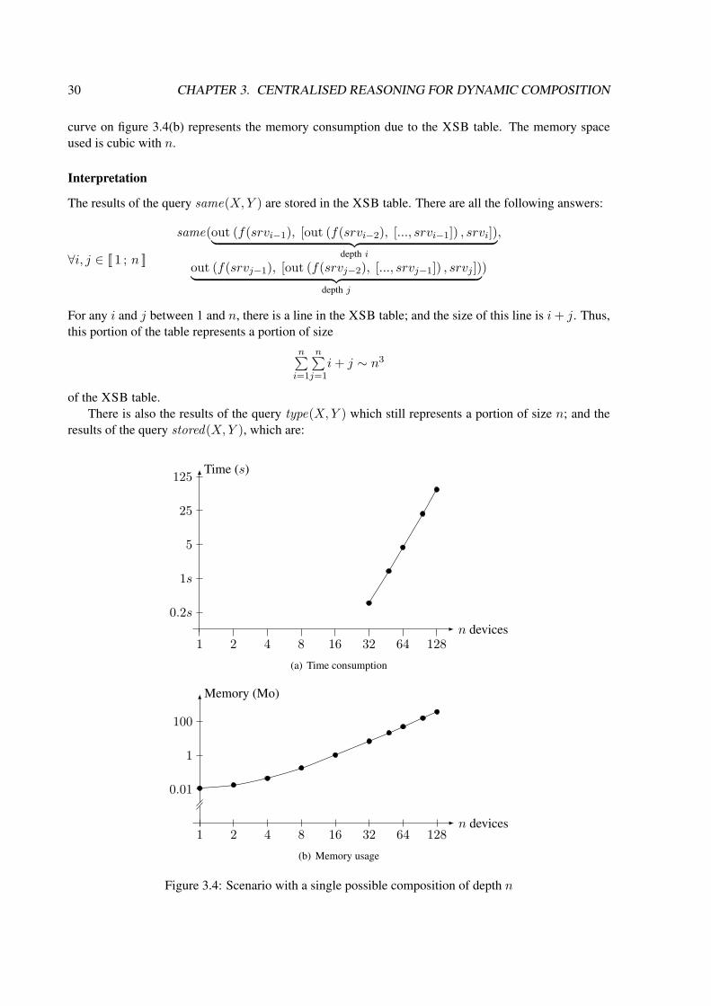
30 CHAPTER 3. CENTRALISED REASONING FOR DYNAMIC COMPOSITION
curve on figure 3.4(b) represents the memory consumption due to the XSB table. The memory spaceused is cubic with n.
Interpretation
The results of the query same(X,Y ) are stored in the XSB table. There are all the following answers:
∀i, j ∈ [[ 1 ; n ]]
same(out (f(srvi−1), [out (f(srvi−2), [..., srvi−1]) , srvi])︸ ︷︷ ︸depth i
,
out (f(srvj−1), [out (f(srvj−2), [..., srvj−1]) , srvj ])︸ ︷︷ ︸depth j
)
For any i and j between 1 and n, there is a line in the XSB table; and the size of this line is i+ j. Thus,this portion of the table represents a portion of size
n∑i=1
n∑j=1
i+ j ∼ n3
of the XSB table.There is also the results of the query type(X,Y ) which still represents a portion of size n; and the
results of the query stored(X,Y ), which are:
0.2s
1s
5
25
125
1 2 4 8 16 32 64 128n devices
Time (s)
(a) Time consumption
0.01
1
100
1 2 4 8 16 32 64 128n devices
Memory (Mo)
(b) Memory usage
Figure 3.4: Scenario with a single possible composition of depth n

3.3. DIFFERENT SCENARIOS 31
Number of devices Time (s) Memory (Ko)1 0.01 112 0.01 184 0.01 448 0.01 18116 0.02 1 Mo32 0.31 6 Mo64 4.3 48 Mo128 68 371 Mo
Table 3.2: Data of the scenario with a single possible composition of depth n
mypc srv1 prn1
srvi prni
srvn prnn
Figure 3.5: Schema of connections in the scenario 3.3.4
∀i ∈ [[ 1 ; n ]] stored(out (f(srvi−1), [out (f(srvi−2), [..., srvi−1]) , srvi])︸ ︷︷ ︸depth i
, srvi)
They represents a portion of size n2 of the XSB table.Thus, the global size of the table is n3.Now, to find all the answers to the query, we have to check every server (n) of the chain and for
everyone, we have to look up in the table of size n3. Thus, the time consumption is quartic.
3.3.4 n possible compositions of depth 2
In this scenario, we have the following connections represented by the graph of connections on figure 3.5:
∀i ∈ [[1;n]]
connected(mypc, srvi)connected(srvi, prni)
There are 2n connections, so that there are n possibilities to print the file myps. For any i, uploadingto the server i and then printing on the printer i is a possible answer to the query.
Statistics and curves
Statistical curves depending on the number of devices are drawn on figure 3.6 in a logarithmic coordinatesystem. The time consumption is represented on the curve on figure 3.6(a). It appears to be cubic with n.The curve on figure 3.6(b) represents the memory consumption due to the XSB table. The memory spaceused is quadratic with n.
Interpretation
The results of the query same(X,Y ) are stored in the XSB table and there are all the following answers:

32 CHAPTER 3. CENTRALISED REASONING FOR DYNAMIC COMPOSITION
Number of devices Time (s) Memory (Ko)8 0.01 5816 0.01 16232 0.04 492 Ko64 0.29 1.7 Mo
128 2.20 6.3 Mo256 17.4 24 Mo512 133 96 Mo
Table 3.3: Data of the scenario with n possible compositions of depth 2
∀i, j ∈ [[ 1 ; n ]] same(out (f(mypc), [myps, srvi]) , out (f(mypc), [myps, srvj ]))
They represent a portion of size n2 of the XSB table.The results of the query stored(X,Y ) are:
∀i ∈ [[ 1 ; n ]] stored(out (f(mypc, [myps, srvi]), srvi))
They represent a portion of size n of the XSB table.Thus, the global size of the table is n2.Finally, to find each of the n final answers to the main query, we have to access the n2-sized table.
Thus, the time consumption is cubic.
0.01
0.1
1
10
100
8 16 32 64 128 256 512n devices
Time (s)
(a) Time consumption
0.11
1001000
8 16 32 64 128 256 512n devices
Memory (Mo)
(b) Memory usage
Figure 3.6: Scenario with n possible compositions of depth 2

3.3. DIFFERENT SCENARIOS 33
mypc srv1 prn1
srvi prni
srvn prnn
Figure 3.7: Schema of connections in the scenario 3.3.5
3.3.5 n2 possible compositions of depth 2
In this scenario, we have the following connections represented by the graph of connections on figure 3.7:
∀i, j ∈ [[1;n]]
connected(mypc, srvi)connected(srvi, prnj)
There are n2 connections and there are n2 possibilities to print the file myps. For any i and j, it ismade possible by the connections to upload the file onto the server i and then to print it on the printer j.
Statistics and curves
Statistical curves depending on the number of devices are drawn on figure 3.8 in a logarithmic coordinatesystem. The curve on figure 3.8(a) represents the time consumption. It appears to be quartic with n. Thecurve on figure 3.8(b) represents the memory consumption due to the XSB table. The memory spaceused is quadratic with n.
Number of devices Time (s) Memory (Ko)1 0.02 11 Ko2 0.02 16 Ko4 0.03 28 Ko8 0.03 58 Ko16 0.07 162 Ko32 0.27 493 Ko64 2 1.7 Mo128 21 6.3 Mo256 280 24.5 Mo512 4217 96 Mo
Table 3.4: Data of the scenario with n2 possible compositions of depth 2
Interpretation
The results of the query type(X, paper) are stored in the XSB table and there are all the followinganswers:
∀i, j ∈ [[ 1 ; n ]] type(out(g(prnj), [out (f(mypc), [myps, srvi])]
), paper)

34 CHAPTER 3. CENTRALISED REASONING FOR DYNAMIC COMPOSITION
0.1s1s
1m
1h
8 16 32 64 128 256 512n devices
Time (s)
(a) Time consumption
0.11
1001000
8 16 32 64 128 256 512n devices
Memory (Mo)
(b) Memory usage
Figure 3.8: Scenario with n2 possible compositions of depth 2
They represent a portion of size n2 of the XSB table.
The results of the query stored(X,Y ) are stored in the XSB table and there are all the followinganswers:
∀i ∈ [[ 1 ; n ]] stored(out (f(mypc), [myps, srvi]) , srvi)
These answers represent a portion of size n of the XSB table.
The results of the query same(X,Y ) are stored in the XSB table and there are all the followinganswers:
∀i, j ∈ [[ 1 ; n ]] same(out (f(mypc), [myps, srvi]) , out (f(mypc), [myps, srvj ]))
They represent a portion of size n2 of the XSB table.
Thus, the size of the whole XSB table is n2.Finally, to find each of the n2 final answers to the main query, we need to access the n2-sized table.
Thus the time consumption is quartic.
3.3.6 2n/2 possible compositions of depth n/2
In this scenario, we suppose that n = 2p. We have the following connections represented by the graphof connections on figure 3.9:
∀i, j ∈ 0, 1 × [[1; p]] srv2i−j+2 ≡ srvij

3.3. DIFFERENT SCENARIOS 35
∀i ∈ 0, 1∀j ∈ [[1; p− 1]]
connected(srvij , srv
ij+1)
connected(srvij , srv1−ij+1)
connected(mypc, srvi1)connected(srvip, prni)
There are only 2×n connections but there are 2p possibilities to print the file. For any x, if i0, . . . , ipis the binary writing of x, then it is made possible by the connections to upload the file onto the server i0,then onto the server i1, ..., and finally onto the server ip before printing it with the printer ip + 1.
mypc srv01 srv0j srv0
p prn1
srv11 srv1j srv1
p prn2
Figure 3.9: Schema of connections in the scenario 3.3.6
Statistics and curves
Statistical curves depending on the number of devices are drawn on figure 3.10. Attention should bepaid to the fact that here the curves are drawn in a semi-logarithmic coordinate system. The curve onfigure 3.10(a) represents the time consumption. It appears to be exponential with n. The curve onfigure 3.10(b) represents the memory consumption due to the XSB table. The memory space used isexponential with n.
0.1s1s
1m
1h
8 10 12 14 16 18n devices
Time (s)
(a) Time consumption
1Ko
1Mo
1Go
8 10 12 14 16 18n devices
Memory
(b) Memory usage
Figure 3.10: Scenario with 2p composition of depth p = bn/2c

36 CHAPTER 3. CENTRALISED REASONING FOR DYNAMIC COMPOSITION
Number of devices Time (s) Memory (Ko)2 0.01 16 Ko4 0.02 48 Ko8 0.06 885 Ko10 0.53 4 Mo12 5.3 18.3 Mo14 48 81.6 Mo16 441 362 Mo18 4503 3897 Mo
Table 3.5: Data of the scenario with 2p compositions of depth p = bn/2c
Interpretation
The results of the query type(X, paper) are stored in the XSB table and there are 2p answers of depth p.Thus, they represent a portion of size p2p of the table.
The results of the query stored(X,Y ) are stored in the XSB table and represent a portion of size p2p
of the table.The results of the query same(X,Y ) are stored in the XSB table and represent a portion of size p22p
of the table.Thus, the size of the whole XSB table is p22p.Then, to find each of the 2p final answers to the main query, we need to access the p22p-sized table.
Thus the time consumption is n22n.
3.4 Summary
This bunch of scenarios shows the behaviour of a quite common scenario with respects to the number ofdevices involved. We have seen with the scenario 3.3.2 how the typing is important. Typing narrows thefield to explore in the description in order to find answers to a query.
There is a summary of all the scenarios seen in this chapter, on table 3.6.
Scenarios 3.3.2 3.3.3 3.3.4 3.3.5 3.3.6possible compositions 1 1 n n2 2n
depth of the compositions 2 n 2 2 n
time consumption n2 n4 n3 n4 n22n
memory usage n n3 n2 n2 n22n
Table 3.6: Summary of all the scenarios
Let us compare the scenario 3.3.2 — where there is a single possible composition of depth 2 — withthe scenario 3.3.3 — where the depth of the single possible composition is n. The time consumption andthe memory usage are multiplied by n2, when the depth of the compositions are only multiplied by an. The comparison between the scenario 3.3.2 and the scenario 3.3.4, considering a number of possiblecompositions multiplied by n, we can see that time and memory are multiplied by n too. Cross verifyingwith the comparison between scenario 3.3.4 and the scenario 3.3.5 which have the same difference as inthe previous comparison, does not show any differences with the memory usage. This can be explain ifwe go back to the scenario and if we see precisely what is stored in memory. There is nothing stored in

3.4. SUMMARY 37
the XSB table that associates a printer and a server in this particular scenario which is the main differencein the graph of connections.

38 CHAPTER 3. CENTRALISED REASONING FOR DYNAMIC COMPOSITION

Chapter 4
Decentralised reasoning for dynamiccomposition of resources
Contents4.1 Reminders and preliminaries . . . . . . . . . . . . . . . . . . . . . . . . . . . . . . 40
4.1.1 Logical description of a device and its functionalities . . . . . . . . . . . . . . 40
4.1.2 Queries . . . . . . . . . . . . . . . . . . . . . . . . . . . . . . . . . . . . . . 42
4.1.3 Example . . . . . . . . . . . . . . . . . . . . . . . . . . . . . . . . . . . . . 44
4.1.4 Relevant devices for a query . . . . . . . . . . . . . . . . . . . . . . . . . . . 45
4.2 Propositional encoding: principles and properties . . . . . . . . . . . . . . . . . . 484.2.1 Encoding of device descriptions and queries . . . . . . . . . . . . . . . . . . . 48
4.2.2 Properties . . . . . . . . . . . . . . . . . . . . . . . . . . . . . . . . . . . . . 52
4.2.3 Examples . . . . . . . . . . . . . . . . . . . . . . . . . . . . . . . . . . . . . 57
4.3 Look-up by decentralised propositional reasoning . . . . . . . . . . . . . . . . . . 594.3.1 Look-up: definition and properties . . . . . . . . . . . . . . . . . . . . . . . . 59
4.3.2 Decentralised computation of Lookup (Q) using SOMEWHERE . . . . . . . . 61
4.4 Heterogeneous descriptions . . . . . . . . . . . . . . . . . . . . . . . . . . . . . . . 62
We assume in this chapter that there is not a central repository of the descriptions of each devices.Instead every device will store their own descriptions. Also, each device has only a few neighbours towhich it is connected. We assume that it cannot exchange data, messages and descriptions but with itsvery neighbours. In this context, the first problem to solve for a device that is queried (by a user or byanother device) is to find in the network the relevant devices whose (possibly composed) functionalitiescan answer the query. This is a difficult problem since each device has a partial knowledge of thenetworked devices and their functionalities.
A flooding strategy could be applied: it would consist of spreading the query from a device to allits neighbours and so on. Each device that could answer part of the query would transmit back thecorresponding answers. All the answers finally received by the initially requested device would haveto be combined. Such a flooding strategy can be applied to P2P systems sharing files (e.g. gnutella)because the queries are simple keywords and the expected answers are single file fitting the keywords ofthe query instead of a set of tuples. In our setting, queries contain variables that can be unified possiblywithin functions in many ways. A flooding strategy would require to spread complex queries and to sendback complex answers that would have to be combined by the queried device, anyway.
39

40 CHAPTER 4. DECENTRALISED REASONING FOR DYNAMIC COMPOSITION
Our approach to answer queries in this decentralised setting is in two steps. First, a look up step thatlooks in the network for the relevant devices (i.e. the ones whose descriptions are sufficient to answerto the query). Then, the second step, which is achieved by the requested device, consists of getting thedescriptions stored in the relevant devices previously found and to locally reason upon them using itslocal PROLOG engine in order to answer the query.
In this chapter, we focus on the look-up step which is the main issue in a decentralised setting — itcorresponds to the (B), (C) and (D) steps in figure 4.6. Our approach can be seen as a flooding strategyapplied to an abstraction in propositional logic of the first-orderquery and the device descriptions. Thisway, queries are abstracted into ‘keywords’ queries where the ‘keywords’ are propositional variables;and device descriptions are abstracted into propositional rules. The look-up is then carried out by adecentralised reasoning in propositional logic which is implemented by the existing SOMEWHERE plat-form [20].
We will begin with a set of reminders and preliminaries to define the set of devices that are relevantto a query. Then we describe the propositional encoding of first-order description that we propose withits properties. Next, we explain how a decentralised reasoning on this encoding with the encoding of aquery can be exploited to find a subset of relevant devices that are still sufficient to get all the answer tothe query. Finally,
4.1 Reminders and preliminaries
4.1.1 Logical description of a device and its functionalities
A device d stores its description: a set of facts and rules in first-order logic. It contains:
• a set of facts representing:
– instanceof relations in the taxonomies: type(d, c);
– subclass relations in the taxonomies: subclassof (c1, c2);
– the assertions of known properties about the device:
∗ type(d, c);∗ connected(d, d′);∗ located(d, l), type(l, cl);∗ inside(l1, l2);∗ stored(o, d), type(o, co);∗ hasfunct(d, f(d)), type(f(d), cf ); where f is a skolem function denoting one of the
functionalities of the device d.
• a set of rules type(d, cd) → hasfunt(d, f(d)), type(f(d), cf ), to assert that every device oftype cd has a functionality of type cf
• a set of rules R describing the functionalities of the device, where a rule r has the form:

4.1. REMINDERS AND PRELIMINARIES 41
r : type(F, T ) Type the functionality∧ hasfunct(D,F ) Specify the device
∧n∧k=1
type(Ik, Tk) Type the inputs
∧ Prec(~I,D) Define preconditions→ type(out(F, [~I]), To) Type the output
∧ Post(~I, out(F, [~I]), D) Define post-conditions
where
– T is the type of the described functionality;– D is the device that has the functionality;– n is the number of inputs for this class T of functionalities;– Ik is one of the inputs;– out is a function representing the output of a functionality F on its inputs [~I];– ~I represents I1, . . . , In;– Prec is a conjunction of preconditions where the inputs and the device D are involved;– Post is a conjunction of post-conditions where the inputs, the output and the device D are
involved;
• a set of rules expressing the inheritance of types. It can also include transitivity, symmetry, reflex-ivity of some properties.
Finally, for a device d, Descr (d) denotes the union of facts and rules mentioned above that describethe device. By extension, for a set D of devices:
Descr (D) =⋃d∈D
Descr (d)
For convenience, for a rule r, we define Descr−1 (r)
d = Descr−1 (r)⇔ r ∈ Descr (d)
For a rule r, Condition (r) denotes the set of the atoms that are present in the premise of the ruler and Conclusion (r) denotes the set of the atoms that are present in the conclusion of the rule r. Weconsider an atomic formula as a rule with an empty condition. Thus, we can extend the definition toatomic formulæ:
Condition (π(t1, t2)) = ∅
Conclusion (π(t1, t2)) = π(t1, t2)
The definition of a predicate π, denoted by Def (π, D), is the union of facts of the form π(t1, t2)and of the rules having an atom π(t1, t2) in their conclusion. As a fact is a rule without conditions, wecan simply write:
Def (π, D) = r ∈ Descr (D) / ∃t1, t2 π(t1, t2) ∈ Conclusion (r)
it is important to note that in a decentralised setting, Def (π, D) may be distributed among severaldevices.

42 CHAPTER 4. DECENTRALISED REASONING FOR DYNAMIC COMPOSITION
Moreover, we define a relation between predicates. A predicate π logically depends on a predicateπ′ among the set of devices D if and only if π′ appears in the conditions of a rule in the definition of π.
π π′ ⇔ ∃r ∈ Def (π, D) , ∃t1, t2 / π′(t1, t2) ∈ Condition (r)
4.1.2 Queries
A query Q is defined by a set of rules (denoted by Def (Q)) of the form:
Def (Q):n∧i=1
Ri(t1i , t2i )→ Q(X0, . . . , Xp)
where tji are terms of the language or variables, Ri are predicates and for all k in [[ 1 ; p ]] it exists i in[[ 1 ; n ]] and j in 1, 2 so that Xk appears in tji . Afterwards X0, . . . , Xp will be denoted by v and calledvariables of interest.
Let D be a set of devices. The answers to the query Q against the union of description Descr (D)— denoted by Answer (Q, D) — is the set of tuples t on Herbrand universe of Descr (D) instantiatedterms for which Q(t) can be logically entailed from the devices descriptions and the definition of thequery.
Answer (Q, D) = t ∈ H(Descr (D))p / Descr (D) ,Def (Q) |= Q(t)
Definition 11 : Derivation treeIn first-order logic, a derivation tree of the query Q with respect to the description of a set of
devices D is a tree that reflects a proof (or a refutation) of Q according to the set of descriptions. Itis denoted by DT (Q, D). Each node of the tree is a (possibly empty) list of atoms. The root node isQ(v). Let N = (A1, . . . , Ak) (with 1 ≤ k) be a node in the tree. Then, for each rules
r =∧pi=1Bi → π1(x, y) ∈ Def (π1, D)
(or facts if p = 0) such that π1(x, y) and A1 are unifiable with σ their Most General Unifier (MGU),the node has a child which is the node N where A1 has been replaced by the Bi and the substitution hasbeen applied:
Biσ, . . . , Bpσ,A2σ, . . . , Akσ
The edge from the node N to this child his labelled by r. If p = 0 (i.e. the atom A1 unifies with afact) then we simply erase A1 from the list and apply the substitution σ. Also if k = 1 and p = 0 (i.e.the node is reduced to one atom unifying with a fact) the child will be an empty clause. Nodes that areempty clause have no children and are called ‘success’ leaves. Nodes that are not empty clause and haveno children are called ‘failure’ leaves. By extension, the set of paths in the tree that end with a successleaf (resp. failure leaf) is called the set of success paths (resp. failure paths) of the tree and is denoted byDT+ (Q, D) (resp. DT− (Q, D)).
Formally, a derivation tree T is a couple made of a node — which is a tuple of atoms — and a list ofsub-trees with the label of the corresponding edge.
T = (R, [(T1, r1), . . . , (Tn, rn)])

4.1. REMINDERS AND PRELIMINARIES 43
[P (X, b)]
[R(X,Y )], P (Y, b)
[P (b, b)]
[P (b, U)], P (U, b)
×
R1
∅X(X/a)
R2
R3
R1
∅X(X/b)
R2
(a) Derivation tree
X Success× Failure(X/b) Substitution
R1. R(X,Y ), P (Y, Z)→ P (X,Z)R2. P (X,X)R3. R(a, b)R4. P (a, c)
(b) Set of rules
Figure 4.1: A derivation tree of a query with respect to a set of rules
where R = (A1, . . . , Ak) is the root of the tree, Ai are atoms, Ti = (Xi, Yi) are derivation trees and riare rules so that:
Descr (D) , R, ri |= Xi
Definition 12 : The height of a derivation tree is:
• zero for a success or a failure
height ((X, ())) = 0
• one more than the height of the highest sub-tree
height ((X, ((T1, r1), . . . , (Tn, rn)))) = 1 + max1≤i≤n
height (Ti)
Definition 13 : We define Rules (T ), the set of all rules that appear in the labels of the edges ofthe tree T .
Rules ((X, ())) = ∅
Rules ((X, ((T1, r1), . . . , (Tn, rn)))) = r1, . . . , rn ∪n⋃i=1
Rules (Ti)
The figure 4.1 shows an example of a derivation tree T of a query with respect to a set of rules andfacts. According to the figure, we have:
height (T ) = 3Rules (T ) = R1, R2, R3

44 CHAPTER 4. DECENTRALISED REASONING FOR DYNAMIC COMPOSITION
4.1.3 Example
The following represents the logical description of three devices. There are parts of the descriptions thatare common for the three devices and concern the taxonomy , the properties of some predicates, theinheritance of types, etc. We introduce them before the description of the devices. Identifiers beginningwith an upper-case letter stand for variables.
r1: subclassof (C, D), type(X, C)→ type(X, D).r2: same(X, Y)→ same(Y, X).
r3:
subclassof (printer, device).subclassof (room, place).subclassof (printing, func).subclassof (download, func).subclassof (paper, data).subclassof (computer, device).subclassof (pc, computer).subclassof (pocketpc, computer).subclassof (file, data).subclassof (postscript, file).
The rule r1 expresses the inheritence of types; the rule r2, the symmetry of the predicate same . Andthe set of facts r3 are an extract of the facts expressing the taxonomies in a logical way.
Consider first, a printer prn, which is located in roomD. Here is its description
type(prn, printer).located(prn, roomD).type(roomD, room).
r4: type(D, printer)→ type(g0(D), printing) ∧ hasfunct(D, g0(D)).
The rule r4 expresses that every printer has a printing functionality. The following rule describes theprinting functionality.
r5:
type(out (G, J) , postscript)∧ type(F, printing)∧ hasfunct(E, G)∧ hasfunct(D, F)∧ connected(E, D)
→ type(out (F, [out (G, J)]) , paper).
The rule r5 describes the printing functionality of a device D. It takes an input of type postscript andprovides an output of type paper provided that the printing device D is connected to a device E that hasa functionality able to output postscript file. Note that out (F, [out (G, J)]) expresses the output of thecomposed functionality.
Consider a PC srv, which is connected to the printer prn.
type(srv, pc)connected(srv, prn)
r6: type(D, pc)→ type(g1(D), download) ∧ hasfunct(D, g1(D)).
The rule r6 expresses that every pc has a download functionality. The rule r7 describes the downloadingfunctionality of a device D. The functionality requires two inputs: a computer S, which is connected to D,

4.1. REMINDERS AND PRELIMINARIES 45
and a file I, which is stored in the computer S and is of a given format C. The functionality provides, asoutput, a file of format C, stored in D and with the same content as I.
r7:
type(I, C)∧type(S, computer) ∧ hasfunct(D, F) ∧ connected(S, D)∧ subclassof (C, file) ∧ stored(I, S) ∧ type(F, download)
→ type(out (F, [I,S]) , C)∧ stored(out (F, [I,S]) , D)∧ same(out (F, [I,S]) , I)
Consider a pocket PC denoted by the constant mypc, storing a postscript file denoted by the con-stant myps and connected to the PC srv. It is described by the following facts.
type(myps, postscript).type(mypc, pocketpc).connected(mypc, srv).stored(myps, mypc).
Finally, consider the query q1 defined by:
hasfunct(D, F) ∧ located(D, roomD)∧ type(out (F, Is) , paper)∧ member(I, Is) ∧ type(I, file) ∧ same(I, myps)
→ q1 (F, Is)
It asks for a functionality F and a list of inputs Is so that
• the device having the functionality F is located in roomD;
• the type of the output of F is paper;
• one of the input from Is is a file which has the same content as the file myps.
An answer to q1 , against the description introduced above, is the following tuple:
(F, Is) = (g0(prn), [out (g1(srv), [myps, mypc])])
where g0(prn) is the printing functionality of prn and its input Is is the output of the functional-ity g1(srv), which is the download functionality of the server srv, applied to the inputs myps and mypc.It expresses that to get myps (stored in mypc) printed in roomD we have to compose the downloadingfunctionality of the PC srv and the printing functionality of the printer prn. Such a composition ispossible because mypc is connected to srv and itself connected to prn.
4.1.4 Relevant devices for a query
Given a query Q asked to a given device d among a set of devices D, the problem is to find a subsetRelevant (Q, D) of D so that the union of their descriptions are sufficient to compute all the answersto Q.
Answer (Q, Relevant (Q, D)) = Answer (Q, D)
The query Q is nothing but a predicate, so we define Relevant (π, D) for any predicate π. We firstdefine Support (π, D), which are the rules or facts that are in the definition of π or in the definition ofany predicate on which π logically depends. We formally define it by induction:

46 CHAPTER 4. DECENTRALISED REASONING FOR DYNAMIC COMPOSITION
Support (π, D) =∞⋃i=0
Supporti (π, D)
where Support0 (π, D) = Def (π, D)
and Supporti+1 (π, D) =⋃ππ′
Supporti (π′, D)
We get the following immediate property:
Support (π, D) = Def (π, D) ∪⋃ππ′
Support (π′, D)
in particular we have
π π′ ⇒ Support (π′, D) ⊂ Support (π, D)
The relevant devices for a predicate π are the devices whose descriptions contain rules or facts be-longing to support of π
Relevant (π, D) = d ∈ D / Support (π, D) ∩Descr (d) 6= ∅
Since the set of devices — and therefore the set of their description — is finite, so is Relevant (π, D)and Support (π, D). More precisely, for any predicate π it exists an integer N such that
Support (π, D) =N⋃i=0
Supporti (π, D)
We prove in lemma 1 that the rules that appear in the labels of the edges of the derivation tree of aninstantiated query belong to the support of the query.
Lemma 1 : Let Q be a query, D a set of devices and t an answer to Q. Then
Rules (DT (Q(t), D)) ⊂ Support (Q, D)
Proof:Since the SLD strategy of resolution — which is implemented in PROLOG engines — is
complete for definite clauses, for any answers t, it exists a deduction of Q(t) from the union ofDescr (D) and Def (Q), which can be summarised by a derivation tree.
Let us prove the inclusion by induction on the height of the derivation tree of Q(t).Basis:Let us assume that the height of the derivation tree of Q(t) is 1. It means that Q(t) unifies
with a fact F , which belongs to the support of Q by definition. Thus,
Rules (DT (Q(t), D)) = F ⊂ Support (Q, D)
Inductive step:Let us assume that for a certain integer n,
if height (DT (Q(t), D)) ≤ n

4.1. REMINDERS AND PRELIMINARIES 47
then Rules (DT (Q(t), D)) ⊂ Support (Q, D)Let us prove the property for a height of n+1. Let us assume that the height of the derivation
tree of Q(t) is n+ 1.
DT (Q(t), D) = (Q(t), [(T1, r1), . . . , (Tk, rk)])
with ∀i height (Ti) ≤ n
if we denote Ti = (πi(ti), Yi) = DT(πi(ti), D
), the inductive hypothesis can be applied and
we deduce that
Rules (Ti) ⊂ Support (πi, D)
Now, Rules (DT (Q(t), D)) =k⋃i=0
ri ∪k⋃i=0
Rules (Ti)
and ri ∈ Support (Q, D)
Also Q πithus Support (πi, D) ⊂ Support (Q, D)
and finally Rules (DT (Q(t), D)) ⊂ Support (Q, D)
♦
Theorem 1 : Let Q be a query, D a set of devices and d a device in D. Then
Answer (Q, Relevant (Q, D)) = Answer (Q, D)
Proof:As Relevant (Q, D) is a subset of D we have one inclusion.
Let us go back to the definitions to prove the other inclusion. Let t be an answer to Q againstthe descrptions of D.
Descr (D) ,Def (Q) |= Q(t)
According to the definition of the derivation tree that correspond to the SLD strategy ofresolution we have
Rules (DT (Q(t), D)) |= Q(t)
Now, we have proved in lemma 1 that
Rules (DT (Q(t), D)) ⊂ Support (Q, D)
And by definition of Relevant (Q, D), we have
Support (Q, D) ⊂ Def (Q) ∪Descr (Relevant (Q, D))

48 CHAPTER 4. DECENTRALISED REASONING FOR DYNAMIC COMPOSITION
We can then deduce
Descr (Relevant (Q, D)) ,Def (Q) |= Q(t)
4.2 Propositional encoding: principles and properties
The principle of our encoding is to abstract the first-order device descriptions and the queries into a setof facts and rules in propositional logic, while preserving some important properties. The main propertyof our encoding is that a propositional backward-reasoning from the encoded query, using the encodeddevice descriptions, leads to the identification of the devices whose first-order descriptions are sufficientto compute the set of all the answers of the first-order query. To relate explicitly a given device d to theencoding of its description, we introduce a particular propositional variable, denoted d?, and we add itas a condition into the propositional rules encoding the first-order rules in the description of d. We callthose propositional variables device propositional variables . We have shown (theorem 3) that the deviceswhose descriptions are sufficient for answering the query are obtained from the propositional implicantsof the encoded query which are conjunctions of device propositional variables. In section 4.2.1, weprovide the encoding function by defining first the encoding of a device, then the encoding of first-order (conjunction of) atoms, and finally the encoding of first-order rules. In particular, the encodingof the class taxonomies is made specific to each device description by encapsulating the inheritancebetween classes into as many propositional rules as there are subclass relations for each first-order atomsinvolving arguments typed by classes. Section 4.2.2 is dedicated to the transfer property (theorem 3) ofour encoding, which shows that the sufficient devices for answering a first-order query can be obtainedby an appropriate decoding of the proper prime implicants of the encoding of the query. The way thistransfer property can be exploited and implemented in a decentralised setting using SOMEWHERE willbe explained in section 4.3.
4.2.1 Encoding of device descriptions and queries
We define the encoding function denoted by Code.
Encoding of a device
For a device d, assuming that d is an identifier of the device in the network, we define
Code (d) = d?
The definition is extended to a set of devices d1, . . . , dn:
Code (d1, . . . , dn) =n∧i=1
d?i
We define also the inverse function:
Decode
(n∧i=1
d?i
)= d1, . . . , dn
In the following, the letter F (or F ′, F0, etc) denotes conjunction of atoms that are made of neitherthe predicate type nor the predicate subclassof ; the letter C (or C ′, C0, etc) denotes conjunction ofatoms which are exclusively made of the predicate type; the letter S (or S′, S0, etc) denotes conjunction

4.2. PROPOSITIONAL ENCODING: PRINCIPLES AND PROPERTIES 49
of atoms which are exclusively made of the predicate subclassof . Atoms of the form type(t, τ)andsubclassof (τ1, τ2) are called typing atoms afterwards.
We distinguish in the description of a device d the following sets of rules:
C0(d) = → type(t, τ) ∈ Descr (d)S0(d) = → subclassof (τ, θ) ∈ Descr (d)T0(d) = C0(d) ∪ S0(d)R0(d) = X ′ → F ∧ C ∈ Descr (d)
T0(d) plays a particular role in the encoding of the descriptions of d and is called the set of typing factsof the device d.
Encoding of an atom
The encoding function comes with two flavours. With the symbol i as a subscript, it provides proposi-tional variables that encode atoms present in the condition of a rule. Those propositional variables arecalled ‘in-propositional variables’ afterwards. With the symbol o as a subscript, it provides proposi-tional variables that encode atom in the conclusion of a rule. Those propositional variables are called‘out-propositional variables’ afterwards.
We first define the encoding of an atom π(t1, t2) — where π is neither the predicate type nor thepredicate subclassof — denoted by Codei (π(t1, t2) |T ) (resp. Codeo (π(t1, t2) |T )) because it dependson the typing atoms of t1 and t2. T is the context of the encoding of π(t1, t2). It is a set of atoms,including the typing of t1 (resp. t2). This typing can be explicit with the predicate type or inferred fromthe domain (resp. range) of the predicate π.
if type(ti, τi) ∈ Tor type(ti, X), subclassof (X, τi) ∈ Tthen Codei (π(t1, t2) |T ) = π.τ1.τ2
i
Codeo (π(t1, t2) |T ) = π.τ1.τ2o
We also encode the atoms of the form type(t, τ) the following way:
Codei (type(t, τ) |T ) = type.τ.Ti
Codeo (type(t, τ) |T ) = type.τ.To
where T denotes the type of the class names. Note that in this case, the encoding is independent of Tand we can write Codei (type(t, τ)) as well.
Encoding of a conjunction of atoms
For convenience, a conjunction of atoms can be seen as a set of atoms. For a conjunction of atoms A,the encoding of A associated with a set of typing atoms is the conjunction of the encoding of each atomof A associated with A ∪ T as set of typing atoms.
Codei (A |T ) =∧a∈A
Codei (a |T ∪A)
Codeo (A |T ) =∧a∈A
Codeo (a |T ∪A)
For instance, suppose we have the following conjunction of atoms.

50 CHAPTER 4. DECENTRALISED REASONING FOR DYNAMIC COMPOSITION
Set of atoms A Set of typing facts T
stored(myps, mypc).type(myps, postscript).connected(mypc, srv)
type(mypc, pocketpc).
then,Codei (A |T ) = stored .postscript.pocketpci ∧ type.postscript.Ti ∧ connected .pocketpc.devicei
The propositional variable connected .pocketpc.devicei is made from the inferred type of srv, which isinferred from the range of the predicate connected .
Encoding of a rule
We now define the encoding of a rule R, which is stored in the device d
R : F ′ ∧ T ′ → F ∧ C
Let T0(d) be the set of typing atoms stored in d. T0(d) represents the context of the encoding of all therules in the description of d.
Code (R |T0(d)) = d? ∧ Codei (F ′ ∧ T ′ |T0(d))→ Codeo (F ∧ C |T0(d) ∪ T ′ )
It is important to note that the encoding of a first-order logic rule provides a propositional logic rule with aconjunction of in-propositional variables in the condition side and with a conjunction of out-propositionalvariables in the conclusion side.
The typing facts that are in C0(d) are particular rules of the form:→ type(t, τ)
then their encoding isCode (type(t, τ)) = d? → type.τ.To
Encoding of the taxonomy
The encoding of a fact→ subclassof (τ, τ ′)
is defined in the context Descr (d).In the following, if it exists the fact→ subclassof (τ, τ ′) in the description of the device d, we say
that τ is a strict subclass of τ ′. The global subclass relation is the transitive and reflexive closure of thestrict subclass relation. τ is a global subclass of τ ′, denoted τ v τ ′ if and only if either τ = τ ′ or it existsτ ′′ such that τ is a strict subclass of τ ′′ and τ ′′ is a global subclass of τ ′. Therefore, if τ v τ ′ appears inthe context of the encoding, it means that it exists τ1, . . . , τn such that for all i between 1 and n− 1, therule→ subclassof (τi, τi+1) belongs to the context of the encoding.
For each rule→ type(t, τ0) such that τ0 is a global subclass of τ we encode all the instantiation onDescr (d) of the following rule:
∀X,C,D type(X,C) ∧ subclassof (C,D)→ type(X,D)
this way:Code (subclassof (τ1, τ2) |→ type(t, τ0), τ0 v τ1 ) = type.τ2.To→ type.τ1.To,
type.τ1.Ti→ type.τ2.Ti,
type.τ0.To → type.τ0.Ti

4.2. PROPOSITIONAL ENCODING: PRINCIPLES AND PROPERTIES 51
device
computer
place
room
(a) The taxonomy used for the schema
located .computer.roomi
located .device.roomi
located .device.placei
located .computer.placei
located .computer.roomo
located .device.roomo
located .device.placeo
located .computer.placeo
(b) Partial encoding of the taxonomy 4.2(a) in the context of the predicate located
Figure 4.2: Example of the encoding of a taxonomy
It is important to pay attention to the fact that rules for the in-propositional variables and for theout-propositional variables are opposite. For instance when a first-order rule conclude on a object typedsay postscript, it will satisfy any query on objects of type file which is a super-class of postscript. In thepropositional encoding the following rule accounts for it:
type.file.To → type.postscript.To
The same way, when a first-order rule has an object typed file in its conditions, then any object typedpostscript which is a subclass of file would satisfy the request. This corresponds to the following rule inthe propositional encoding:
type.postscript.Ti → type.file.Ti
When other predicates appear in Descr (d) we encapsulate the subclass relation in the propositionalencoding in a similar way. More precisely, for each predicate π we define:
Code
→ subclassof (τ1, τ2)
∣∣∣∣∣∣ π(td, tr),
type(td, τd), τd v τ1,type(tr, τr), τr v α
= π.τ1.α
i→ π.τ2.αi,
π.τ2.αo → π.τ1.α
o,π.τd.τr
o → π.τd.τri
Code
→ subclassof (τ1, τ2)
∣∣∣∣∣∣ π(td, tr),
type(td, τd), τd v α,type(tr, τr), τr v τ1
= π.α.τ1
i→ π.α.τ2i,
π.α.τ2o→ π.α.τ1
o,π.τd.τr
o→ π.τd.τri
Finally, the encoding of a rule→ subclassof (τ1, τ2) in the context of Descr (d) is obtained bu takingthe union of all the above encoding:
Code (→ subclassof (τ1, τ2) |Descr (d)) =⋃
A⊂Descr(d)
Code (→ subclassof (τ1, τ2) |A)

52 CHAPTER 4. DECENTRALISED REASONING FOR DYNAMIC COMPOSITION
Figure 4.2(b) shows the encoding of the subclass relations in the taxonomy of figure 4.2(a) in thecontext of a description containing
located(pc1, roomD), type(pc1, computer), type(roomD, room)
The propositional rules are represented as edges in a graph where vertices are propositional variables andarrows between two propositional variables a and b denotes a rule a→ b.
Encoding of a whole description
The encoding of the description of a device d is the union of the encoding of its rules and the encodingof its taxonomy description.
Code (Descr (d)) =⋃
R∈R0(d)
Code (R |T0(d)) ∪⋃
C∈C0(d)
Code (C) ∪⋃
S∈S0(d)
Code (S |Descr (d))
Afterwards, we will note ∆ the union of the encoding of the description of all devices.
∆ =⋃d∈D
Code (Descr (d))
Encoding of queries
A query is defined by a set of rules. Thus, the encoding of a query is the union of the encoding of eachrule from its definition:
Code (Q) =⋃
R∈Def(Q)
Code (R)
4.2.2 Properties
The following properties of the encoding are going to be useful to the transfer property.
Property 1 : This property shows that for a predicate offered in conclusion of a first-order rule, theassociated out-propositional variable entails the corresponding in-propositional variable. It expresses therelay race composition of functionalities in the propositional side.
If there exists r ∈ Descr (d) such that π(t1, t2) ∈ Conclusion (r) with τ1 (resp. τ2) being the typeof t1 (resp. t2), then
∆, π.τ1.τ2o |= π.τ1.τ2
i
Proof:Let θ1 be a strict super-class of τ1. Then
Code (subclassof (τ1, θ1) |Descr (d)) ∈ ∆
Now, π(t1, t2) ∈ Descr (d)type(t1, τ1) ∈ Descr (d)type(t2, τ2) ∈ Descr (d)
subclassof (tau1, θ1) ∈ Descr (d)

4.2. PROPOSITIONAL ENCODING: PRINCIPLES AND PROPERTIES 53
So, from the definitions we have:
π.τ1.τ2o → π.τ1.τ2
i ∈ Code (subclassof (τ1, θ1) |π(t1, t2), type(t1, τ1))
♦
Property 2 : We extend the previous property throughout subclass relations.Let τ1, τ2, θ1, θ2 be class names such that τ1 v θ1 or θ1 v τ1, and τ2 v θ2 or θ2 v τ2. Then,
∆, π.τ1.τ2o |= π.θ1.θ2
i
Proof:First case, τ1 v θ1 and τ2 v θ2:From the definition of the encoding we have
∆, π.τ1.τ2o |= π.τ1.τ2
i
and ∆, π.τ1.τ2i |= π.θ1.θ2
i Q.E.D.
Second case, θ1 v τ1 and θ2 v τ2:From the definition of the encoding we have
∆, π.τ1.τ2o |= π.θ1.θ2
o
and ∆, π.θ1.θ2o |= π.θ1.θ2
i Q.E.D.
Third case, θ1 v τ1 and τ2 v θ2:From the definition of the encoding we have
∆, π.τ1.τ2o |= π.θ1.τ2
o
and ∆, π.θ1.τ2o |= π.θ1.τ2
i
and ∆, π.θ1.τ2i |= π.θ1.θ2
i Q.E.D.
The last case and the previous one are symmetrical.
♦
Property 3 : LetA be a conjunction of atoms, T a set of typing atoms and σ any substitution. Then
∆,Codeo (A |T ) |= Codeo (Aσ |T )∆,Codei (Aσ |T ) |= Codei (A |T )
Proof:For an atom π(t1, t2), where π is not the predicate type, as we treat terms in the encoding
regardless of the presence of variables, we have the equality between encoding with or withoutsubstitutions. Thus, for the atom π(t1, t2), the property is straightforward.
For an atom type(t, X) where the class name is a variable, a substitution may affect thevariable X. And as Xσ v top and
Codeo (type(t, X) |T ) = type.top.To
Codeo (type(t, Xσ) |T ) = type.Xσ.To
Codei (type(t, X) |T ) = type.top.Ti

54 CHAPTER 4. DECENTRALISED REASONING FOR DYNAMIC COMPOSITION
Codei (type(t, Xσ) |T ) = type.Xσ.Ti
we have the result.
♦
Property 4 : Let A, B and C be conjunctions of atoms. Then
Codei (A ∧B |C ) = Codei (A |B ∪ C ) ∧ Codei (B |A ∪ C )
Proof:Straightforward with the definition of the encoding for conjunction of atoms.
♦
Property 5 : Let A, B and C be conjunctions of atoms. Then
∆,Codei (A |B ∪ C ) |= Codei (A |C )
Proof:Let us prove it for an atom a and two conjunctions of atoms B and C.First case: a = type(t, τ). In this case we have,
Codei (type(t, τ) |B ∪ C ) = Codei (type(t, τ) |C )
Second case: a = π(t1, t2), with θ1 (resp. θ2) the domain (resp. the range) of the predicate π.
Sub-case 1:for all k if type(tk, τk) ∈ Cor type(tk, X), subclassof (X, τk) ∈ Cthen Codei (π(t1, t2) |B ∪ C ) = π.τ1.τ2
i = Codei (π(t1, t2) |C )
Sub-case 2:for all k if type(tk, τk) 6∈ B ∪ Cor type(tk, X), subclassof (X, τk) 6∈ B ∪ Cthen Codei (π(t1, t2) |B ∪ C ) = π.θ1.θ2
i = Codei (π(t1, t2) |C )
Sub-case 3:for all k if type(tk, τk) ∈ B \ Cor type(tk, X), subclassof (X, τk) ∈ B \ Cthen Codei (π(t1, t2) |B ∪ C ) = π.τ1.τ2
i
Codei (π(t1, t2) |C ) = π.θ1.θ2i
Sub-case 4:if type(t1, τ1) ∈ B \ Cor type(t1, X), subclassof (X, τ1) ∈ B \ Candif type(t2, τ2) ∈ Cor type(t2, X), subclassof (X, τ2) ∈ Cthen Codei (π(t1, t2) |B ∪ C ) = π.τ1.τ2
i
Codei (π(t1, t2) |C ) = π.θ1.τ2i

4.2. PROPOSITIONAL ENCODING: PRINCIPLES AND PROPERTIES 55
Sub-case 5: Similar to the sub-case 4Finally, as for all k we have τk v θk we can conclude for an atom a:
∆,Codei (a |B ∪ C ) |= Codei (a |C )
The extension for a conjunction of atoms is straightforward.
♦
Property 6 : Let A, B and C be a conjunction of atoms. Then
∆,Codei (A ∧B |C ) |= Codei (A |C ) ∧ Codei (B |C )
Proof:This property is a corollary of the property 4 and property 5.
♦
The definition 14 introduces the notion of proper prime implicants which is central for the transferpropoerty.
Definition 14 : Proper prime implicant with respect to a theory. Let Γ be a clausal theory and qbe a cube (conjunction of literals). A cube m is said to be:
• a prime implicant of q with respect to Γ if and only if Γ,m |= q and for any other cubes m′, ifΓ,m′ |= q and m |= m′ then m ≡ m′.
• a proper prime implicant of q with respect to Γ if and only if it is a prime implicant of q withrespect to Γ and Γ 6|= ¬m.
The set of proper prime implicants of q with respect to Γ is denoted by
Ppi (q,Γ)
Theorem 2 : Transfer propertyLet Q be a query, D a set of devices and ∆ the union of the encoding of the descriptions of all device
in D. Let t an answer to Q, and P = (r1, . . . , rn) be a success path of the derivation tree of Q(t). Let dibe the device that stores the rule ri.
Then,
(n∧i=1
d?i
)is a proper prime implicant of Code (Q) with respect to ∆
Proof:Let us proceed by induction on the length of the path (r1, . . . , rn). We consider the proposi-
tional variable q, the encoding of the query Q
Basis:Let us assume that the length of the path P is 1. It means that Q(t) unifies with a fact F =
π(t1, t2) stored in the device d1, where the type of t1 is τ1 and the type of t2 is τ2.

56 CHAPTER 4. DECENTRALISED REASONING FOR DYNAMIC COMPOSITION
π(t1, t2), type(t1, τ1), type(t2, τ2) ∈ Descr (d1)
Thus Code (Q) is of the form π.θ1.θ2i and as Q(t) unifies with F we have τ1 v θ1 and τ2 v θ2.
Then, with the property 2, we have:
∆, π.τ1.τ2i |= π.θ1.θ2
i
It exists in the encoding of the description of d1 the following rule π.τ1.τ2o → π.τ1.τ2
i.
Then ∆, π.τ1.τ2o |= π.θ1.θ2
i
and as F belongs to Descr (d1), the following rule d?1 → π.τ1.τ2o belongs also to ∆, so:
∆, d?1 |= π.τ1.τ2o
and finally ∆, d?1 |= Code (Q)Therefore, d1 is the device that stores the rule r and d? is a proper prime implicant of Code (Q)with respect to ∆.
Inductive step:Let us assume that for a certain integer n, for any query Q and for any success paths P =
(r1, . . . , rn) in the derivation tree of Q(t) so that the length of P is equal to n, if di =Descr−1 (ri), we have that (
n∧i=1
d?i
)∈ Ppi (Code (Q) ,∆)
Let P = (r1, . . . , rn+1) be a success path of length n+ 1 in the derivation tree of Q(t). LetA1, . . . , An the set of atoms of the successor of the root node in the success path. Let us considerCode (
∧ni=1Ai). Afterwards, di = Descr−1 (ri).
We have r1 = F ′ ∧ T ′ → F ∧ CandCode (r1 |T0(d1)) =
d?1 ∧ Codei (F ′ ∧ T ′ |T0(d1))→ Codeo (F ∧ C |T0(d1) ∪ T ′ )
in particular, one of the atoms in the conclusion of r1 (say F1 = π(t1, t2)) unifies with A1 (sayπ(u1, u2)) and their MGU is σ. Then after the deletion of A1 by the rule r1 we have
F ′σ, T ′σ,A2σ, . . . , Anσ
Moreover, in our model everything is typed at least implicitly, for each i, inF ′σ, T ′σ,A2σ, . . . , Anσ, either there is type(tiσ, τi) and type(uiσ, τ ′i) or they are implicit.As it is a success path, both hold. And as uiσ = tiσ, it results that it is the same object that istyped twice. So for each i either τi v τ ′i or τ ′i v τi. Thus, in the propositional side, the property 1assures that it exists a set of rules in ∆ such that:
∆,Codeo (F1σ |T ′ ∪ C ∪ T0(d1)) |= Codei (A1σ |⋃ni=2 Ai )
With the property 3 we can remove the substitution and we have:

4.2. PROPOSITIONAL ENCODING: PRINCIPLES AND PROPERTIES 57
∆,Codeo (F1 |T ′ ∪ C ∪ T0(d1)) |= Codeo (F1σ |T ′ ∪ C ∪ T0(d1))∆,Codei (A1σ |
⋃ni=2 Ai ) |= Codei (A1 |
⋃ni=2 Ai )
and because Code (r1 |T0(d1)) belongs to ∆, we have
∆, d?1 ∧ Codei (F ′ ∧ T ′ |T0(d1)) |= Codeo (F1 |T ′ ∪ C ∪ T0(d1))
and so, ∆, d?1 ∧ Codei (F ′ ∧ T ′ |T0(d1)) |= Codei (A1 |⋃ni=2 Ai )
Now according to the property 4 we have
Codei (A1 |⋃ni=2 Ai ) ∧ Codei (
∧ni=2Ai |A1 ) = Codei (
∧ni=1Ai)
Therefore, Codei (F ′ ∧ T ′ |T0(d1)) ∧ Codei (∧ni=2Ai |A1 ) ∧ d?1 is an implicant of
Codei (∧ni=1Ai) with respect to ∆.
Now, the set of atoms F ′σ, T ′σ,A2σ, . . . , Anσ resulting from the deletion of A1 is encodedinto the set of propositional variables
Codei (F ′σ ∧ T ′σ ∧∧ni=2Aiσ)
According to the property 3 we have:
Codei (F ′σ ∧ T ′σ ∧∧ni=2Aiσ) = Codei (F ′ ∧ T ′ ∧
∧ni=2Ai)
According to the property 6 we have:
∆,Codei (F ′ ∧ T ′ ∧∧ni=2Ai) |= Codei (F ′ ∧ T ′) ∧ Codei (
∧ni=2Ai)
Until now we have proved the following:
∆, d?1,Codei (F ′σ ∧ T ′σ ∧∧ni=2Aiσ) |= Codei (
∧ni=1Ai)
Now, P ′ = (r2, . . . , rn+1) the sub-path of P satisfies the inductive hypothesis. Thus, wehave:
(∧n+1i=2 d
?i
)is a proper prime implicant of Code (F ′σ ∧ T ′σ ∧
∧ni=2Aiσ) with respect to
∆
4.2.3 Examples
An example with two computers pc1 — which is located in a room roomD — and srv1 — which islocated in a building batC — is described in table 4.1. The encoding of their description is representedfigure 4.3 by a graph where vertices are propositional variables and arrows between two propositionalvariables a and b denotes a propositional rule a → b in the encoding. From the example, a query Q— asked to the device d1 — in logic can be:
located(X, Y) ∧ type(Y, room)→ Q(X)
and its encoding:
d?1 ∧ located .device.roomi → q
Figure 4.4 shows the derivation tree of the above first-order queryQwith respect to the first-order de-scription shown in table 4.1. Thus, using the encoding, the set of device propositional variable implicants

58 CHAPTER 4. DECENTRALISED REASONING FOR DYNAMIC COMPOSITION
d?1
located .computer.roomo
located .computer.roomi
located .computer.placei
ρ14
located .device.roomi
located .device.placei
ρ15
ρ16
ρ112
located .computer.placeo
located .device.placeo
ρ111
ρ18
located .device.roomo
ρ110 ρ1
1
type.computer.To
type.computer.Ti
type.device.Ti
ρ114
ρ116
type.device.To
ρ117
ρ12
type.room.To
type.room.Ti
type.place.Ti
ρ113
ρ115
type.place.To
ρ118
ρ13
ρ17
ρ19
Figure 4.3: The encoding of a description shown in a graph
Table 4.1: Descriptions of two devices and their encoding(a) Rules that enable the inheritance of types
R0: subclassof (C, D), type(X, C)→ type(X, D)
(b) Description of a computer
R11: type(pc1, computer)
R12: type(roomD, room)
R13: subclassof (room, place)
R14: subclassof (computer, device)
R15: located(pc1, roomD)
(c) Description of a server
R21: type(srv1, computer)
R22: type(batC, building)
R23: subclassof (building, place)
R24: subclassof (computer, device)
R25: located(srv1, batC)

4.3. LOOK-UP BY DECENTRALISED PROPOSITIONAL REASONING 59
of the encoding of Q is d?1 as shown in figure 4.5
4.3 Look-up by decentralised propositional reasoning
We exploit the transfer property of the propositional encoding to retrieve a (possibly strict) subset ofthe relevant devices for a query Q. In section 4.3.1 we show (Theorem 3) that such a subset, denotedLookup (Q) can be obtained by decoding the proper prime implicant of the encoding of Q that aremade of device propositional variables only. In section 4.3.2, we show how to use SOMEWHERE for adecentralised implementation of the computation of Lookup (Q).
4.3.1 Look-up: definition and properties
Definition 15 : Let Ppi? (q,∆) be the set of proper prime implicants of q made of device propositionalvariables.
Ppi? (q,∆) = n∧i=1
d?i ∈ Ppi (q,∆)
Let Lookup (Q) be the set of devices decoded from Ppi? (Code (Q) ,∆).
Lookup (Q) =⋃
P∈Ppi?(Code(Q),∆)
Decode (P )
The following theorem states that the look up method consisting in computing Lookup (Q) is soundand complete. That is to say, for a query Q, an answer is found using only the description of the devicesof Lookup (Q) if and only if it is a correct answer that would have been found also using the whole setof available devices.
Theorem 3 : Let Q be a query and D a set of devices
Answer (Q, D) = Answer (Q, Lookup (Q))
Proof:As the Lookup (Q) is a subset of the devices, the lookup is sound.The other inclusion of the theorem can be rewritten as:
∀t Descr (D) |= Q(t) → Descr (Lookup (Q)) |= Q(t)
Let us consider the derivation tree of Q(t). Let P = (r1, . . . , rn) be the success path and dithe device that stores the rule ri in its description. Then according to the theorem 2
Code
(n⋃i=1
di
)∈ Ppi? (Code (Q) ,∆)
From the definition of Lookup we deduce:n⋃i=1
di ∈ Lookup (Q)

60 CHAPTER 4. DECENTRALISED REASONING FOR DYNAMIC COMPOSITION
Q(v)
[located(X, Y)],type(Y, room)
[type(roomD, room)]
∅X(X/pc1)(Y/roomD)
R12
R15
[type(batC, room)]
[subclassof (Z, room)],type(batC, Z)
×
R0
R25
Figure 4.4: Derivation tree of the query Q with respect to the rules in table 4.1
Code (Q)
[located .device.roomi],type.room.Ti
[located .computer.roomi],type.room.Ti
[located .computer.roomo],type.room.Ti
d?1, [type.room.Ti]
d?1, [type.room.To]
d?1
ρ13
d?1, type.place.To
ρ118
ρ115
ρ11
[located .computer.placeo],type.room.Ti
located .device.placeo,
[type.room.Ti]
located .device.placeo,[type.room.To]
located .device.placeo, d?1
ρ13
located .device.placeo,type.place.To
ρ118
ρ115
ρ111
ρ18
[located .device.roomo],type.room.Ti
ρ110
ρ112
ρ16
ρ19
Figure 4.5: Propositional implicants of Code (Q) with respect to the encoding of the rules

4.3. LOOK-UP BY DECENTRALISED PROPOSITIONAL REASONING 61
and thus, Descr
(n⋃i=1
di
)⊂ Descr (Lookup (Q))
Now we are in a success path so we have
Descr
(n⋃i=1
di
)|= Q(t)
And therefore, Descr (Lookup (Q)) |= Q(t)
The important point is that, while the look-up method is complete, Lookup (Q) can provide a strictsubset of Relevant (Q, D). It is shown using the example in table 4.1. From figure 4.4 we see thatRelevant (Q, D) is the set of d1 and d2 — because the rules appearing in the label of the edges of thederivation tree come from d1 and d2 — while in figure 4.5, we can see that Lookup (Q) is the singletond1 — because d?1 is the only proper prime implicants of the query made of device propositional variables.
4.3.2 Decentralised computation of Lookup (Q) using SOMEWHERE
Figure 4.6 illustrates the possible implementation of the look-up method in a decentralised setting byadding layers on top of SOMEWHERE deployed in each device. the process in the centralised setting.The top layer, deals with the user interface. The step 1 (resp. step A) represents the translation of thedescription (resp. a query) from the high-level language to the first-order logic. The intermediate layerdeals with the first-order logic description and reasoner. The step 2 (resp. step B) represents the encoding
Propositional logic
2
Code (Descr (d))
SO
MEW
HER
EB
D
C
First-order logic
1
Descr (d)
PRO
LO
G
A
F
E
High-level language
DescriptionQuery
Answer
Figure 4.6: Schema of the whole process in a device

62 CHAPTER 4. DECENTRALISED REASONING FOR DYNAMIC COMPOSITION
of first-order description (resp. first-order query). The bottom layer is the propositional logic encodingand reasoner handled by SOMEWHERE.
SOMEWHERE is a fully decentralised propositional logic reasoner. It is deployed on each deviceof the opportunistic network in a form of a piece of JAVA code. The SOMEWHERE layer computesthe proper prime implicants of a conjunction of propositional variables with respect to a decentralisedpropositional theory. In our context, the conjunction of propositional variables is the encoded queryand the propositional theory is the global theory ∆. Some of the propositional variables can be definedin SOMEWHERE as target variables and we can restrict the computation of proper prime implicants tothose target variables. In our context, device propositional variables are the target variables. Therefore,the look-up can be achieved by the SOMEWHERE platform (step C).
According to the transfer property (Theorem 2 in section 4.3.1), the decoding of the result returnedby SOMEWHERE triggered on the queried device provides the result of Lookup (Q). Therefore, thequeried device can download the first-order description of the devices selected by the look-up process(step D), and locally computes using the PROLOG engine the answers to the query with respect to to theselected descriptions (step E).
4.4 Heterogeneous descriptions
So far in this chapter, we have assumed that the descriptions between devices were homogeneous, i.e. us-ing a common taxonomy shared by every devices. We describe in this section what changes must be donein the encoding and the look-up process if we allow heterogeneous descriptions. Throughout this section,we assume that class names appearing in the taxonomy of a device are prefixed with the identifier of thatdevice, so that similar class names between taxonomies are disambiguated.
Mappings between heterogeneous taxonomies have been introduced in section 2.7. They establisha subclass relation between class names in the taxonomies of two different devices. In a decentralisedsetting, we just have to add the mappings in the device description: in the description of a device d,we add the mappings, denoted by M0(d) the subset of Descr (d) made of the predicate subclassof andcontains foreign class names. M0(d) is a subset of S0(d) and therefore it is encoded the same way.Therefore, the lookup method presented in section 4.3 based on propositional encoding applies withoutchanges to the case of heterogeneous descriptions.

Bernard de Chartres said that we are like dwarfs sitting on theshoulders of giants. We see more, and things that are moredistant, than they did, not because our sight is superior orbecause we are taller than they, but because they raise us up,and by their great stature add to ours.
Metalogicon III, Jean de Salisbury (1115–1180)
Chapter 5
Related Work and Conclusion
Contents5.1 Semantic Approach of Dynamic Web Services Composition . . . . . . . . . . . . . 64
5.2 Web Service Composition via Planning . . . . . . . . . . . . . . . . . . . . . . . . 67
5.3 Logic based language for Web services composition . . . . . . . . . . . . . . . . . 68
5.4 Conclusion . . . . . . . . . . . . . . . . . . . . . . . . . . . . . . . . . . . . . . . . 71
We focus this chapter on comparing our work to previous existing work on dynamic Web servicecomposition. A Web service [7] is an application that can be described, published, and invoked overthe network by using standards network technologies. Those characteristics match the characteristics ofdevices and functionalities. In our model Web services can be treated as logical devices while embeddedservices are equivalent to functionalities.
In the last decade, Web service composition problems and Web service discovery problems havebeen addressed (e.g. see [8, 19] for surveys). The Web service discovery problem is to fulfil a request ofa Web service that has initial input parameters and desired output. The Web service composition problemoccurs when no single Web service can satisfy the user request whereas a composite Web service— madeof a combination of either simple or composite Web services — could satisfy it. To achieve this goal, alarge number of research works has been carried out :
• using planning [15, 25];
• given a model to express composition between Web services to verify compositions [10, 18];
• to effectively build composition of Web services down to a lower granularity of the descriptions.
Some works (e.g. [4, 6, 25]) compose Web services by mingling their behaviour and execution, whichneeds to describe the Web services at a low level.
Several works on Web service composition are based on predefined patterns [10, 26] or bindingsbetween services that are known beforehand [3]. A more challenging problem, which is the one weaddress, is to compose services dynamically, on demand. Few works address it. We structure this chapteraccordingly, by first situating our approach with respect to semantic approaches, then with respect toapproaches based on planning and finally with respect to logic-based approaches. Note that those threeapproaches are not disjoint and some of the works detailed here can be ranked among more than onesection.
63

64 CHAPTER 5. RELATED WORK AND CONCLUSION
5.1 Semantic Approach of Dynamic Web Services Composition
The semantic approach aims to give resources well-defined meaning and to make them machine-under-standable. Then, resources can be shared and processed by automated tools as well as by human users.The introduction of semantics in Web service composition is the continuity of the Semantic Web, whichvision was first introduced by [5].
The semantics is described by standard languages including :
• Uniform Resource Identifier (URI) a fundamental component of current Web. It allows to uniquelyidentify resources as well as relations among resources;
• eXtensible Markup Language (XML) provides a syntactical interoperability on Web. It is theuniversal format for structured documents and data on the Web;
• RDF leverages URI and XML to allow documents being described in the form of metadata bymeans of resources, properties, and statements;
• RDFS is an extension of RDF, which defines a simple modeling language on top of RDF. Itenables the representation of class, property and constraint while RDF allows the representationof instances and facts, thus making it a lightweight ontology language. While RDF and RDFSare different, they are combined together to form the basic language for knowledge representationdenoted as RDF(S);
• Web Ontology Language (OWL) use the RDF(S) as a starting point and extend it to a more ex-pressive powered ontology specification language for the description of the semantic Web.
Our language is an extension of RDF(S) that make uses of function. In chapter 2 we expressed ourlanguage in RDF(S) whenever it was possible.
We compare our work to some previous work introducing semantics for data in Web service composition.The first one introduce the concept of semantic value, and the second builds an ontology upon which thecomposition is made.
In [13], Web service composition satisfy two conditions:
• Web services must agree on the meaning of the exchanged data in order to build consistent com-position;
• semantic-data conflicts — such as incompatibility of types or differences in the unit used — mustbe resolved using context.
The data conflicts arisen by the composition make [13] resolve these conflicts by using the conceptof semantic value introduced in [24]. A semantic value is the association of a simple value (like ‘5’ asan integer) and a semantic information — named the context — to ease the contextual understanding(e.g. “5(currency = euro)” describes 5 units of currency of type euros). The context is a set of propertieswhere each property is assigned to a semantic value. This definition is recursive. For instance a rent canbe expressed like:
640 (Periodicity = ‘monthly’(FirstIssueDate = ‘15 Jan’), Currency = ‘Euros’).
Here, the value 640 has two properties: Periodicity and Currency. The value of the former property isalso a semantic value having the property FirstIssueDate. The semantics of 640 can thus be interpretedas a monthly rent of 640 euros with a beginning on January 15. Upon such a definition, the conceptof semantic mediator is introduced in [17]. A semantic mediator is triggered during a Web service

5.1. SEMANTIC APPROACH OF DYNAMIC WEB SERVICES COMPOSITION 65
composition and execution and it is not embedded in any of the Web services involved in the composition.It is rather an independent component that permits conversion and comparison between semantic values.
In our approach, data are typed and can have properties (e.g. stored) . They may have a propertythat value them. For instance the taxonomy of data-type can contain “Euro” as a sub-type of “Currency”and a data object — whose value-property is for instance ‘5’ — can be declared to be an instance of“Euro”. Finally, the semantic mediator is covered by the mappings between taxonomies when there isno conversion of values or by a functionality that makes the conversion.
To make sure that different users (machine or human) have a common understanding of the terms,ontologies in which terms are described, and which establish a joint terminology are usually adopted.
For a particular form of Web services called ‘Data-providing’ Web services, [4] addresses the prob-lem of composition by defining an ontology. Data-providing Web services (as opposed to Effect-providingWeb services) corresponds to our functionalities without post-condition. They define an ontology by a6-tuple:
1. a set of classes C;
2. a set of data-types L;
3. a set of data-type properties DP ;
4. a set of object properties OP ;
5. a sub-class relationship between classes (C × C);
6. and a sub-property relationship between homogeneous properties (OP ×OP ∪DP ×DP ).
A query is defined on the instance graph of an ontology by a 3-tuple:
1. a backbone : a sequence of the form
?c1(C1).Ψ.p1.2.?c2(C2).Ψ.p2.3 . . .Ψ.pn−1.n.?cn(Cn)
where
• ci is a variable of type Ci, which is a class of the ontology;• pi,j is an object property involving ?ck 1 ≤ k ≤ n;• Ψ is a linking operator. Instances of ?ci must satisfy all of the conditions specified by Ψ;
2. the constraints set imposed on data-type properties of the variables in the backbone;
3. the output set including output variables.
Implemented in the RDF query language SPARQL, an example of a query that means ‘For a patientP1 who takes a medication termed “Some Stuff”, what are the tests they had to perform’ could be :
Q1 :Backbone =?T1(type : Test).[HasTest]−1.?P1(type : Patient).[TakeDrugs].?M1(type : Drugs)Ct = $M1(Name = “Some Stuff′′),Out = ?T1(Result)
They model the Data-Providing Web services as RDF Parametrised views over an OWL ontology. Aparametrised view is a predicate WSi(Ci) called the view head and a 4-tuple called the view body:

66 CHAPTER 5. RELATED WORK AND CONCLUSION
1. a backbone that includes both the variable set C (of classes types) linking input and the output ofthe service, and the object properties set OP relating the different variables in C;
2. A set of constraints imposed on the data-type properties of C such that they are not required inputsof the service;
3. Necessary literals for the service invocation;
4. Output literals.
The parametrised view permits to catch the semantic relation holding between the inputs (literalsfor the service invocation) and the outputs. For instance, a Web services that provides the name of thepatients that take a certain medication is written as follow :
WS4(Patient(Name)) : −?Patient.[TakeDrugs].?DrugCt : ∅In : $Drug(Name)Out : ?Patient(Name)
The resolution of the query is based on the parametrised views of the services. In order to satisfya query, a set of services is selected and the union of their backbones has to cover the backbone of thequery. It means that the requested data items are provided and the query’s constraints list is satisfied withthe union of the constraints of the selected services. As a matter of fact, the composition is guided bythe structure of the query’s backbone. The form of the composed Web services expected as an answer tothe query is known beforehand. Thus, with this approach, one may fail finding composition even if thereis possible composition that would provide the data items requested without satisfying the constraints ofthe backbone. In our approach the query is more flexible as it is expressed directly in first-order logic(without the constraint of the backbone, a sequence of a particular form) used here.
A rule based composition is done in [16] by generating composite services from high-level declarat-ive description. Rules (called composability rules) are used to determine whether two services are likelyto be composed. The approach consists in four phases:
1. Specification: a high-level description of the desired compositions using Composite Service Spe-cification Language (CSSL), allowing semantic features and specification of the control flowbetween composite service operations.
2. Match-making: composability rules are used to generate composition plans conform to the re-quests. This phase checks purpose composability and category composability between a compos-ite service operation and a component service operation. It checks also quality composability andmessage compatibility (leading to a one-to-one mapping between messages).
3. Selection: if more than one plan is generated, a selection is made based on quality of compositionparameters like ranking, relevance (also called soundness) and completeness;
4. Generation phase.
The composability rules checks different aspects of the composition that are equivalent to the as-sembly line composition and relay race composition in our approach and they are expressed and checkedby the reasoner during the answering of a query.

5.2. WEB SERVICE COMPOSITION VIA PLANNING 67
5.2 Web Service Composition via Planning
There are many research tackling Web service composition problem via planning. A planning problemcan be described by a set S of all possible states of the world, a set S0 of initial state, a set G of goalsstates the planning system attempts to reach. a set A of actions planner can perform changing one stateto another in the world and a relation Γ ⊂ S × A × S which defines the preconditions and effects forthe execution of each action. In the terms of Web services, S0 (resp. G) is the initial states (resp. thegoal states) specified in the requirement of Web services. A represents a set of available services and Γdenotes the state change function of each service.
An automated composition task using planning methods is also used in [25] that build a new com-posed service (i.e. the state transition system), given the OWL-S process model description of n availableservices.
A state transition system is a 6-tuple:
1. a set S of states;
2. a set A of actions;
3. a set O of observations;
4. a set I of initial states, subset of S (I 6= ∅);
5. a transition function T : S × A 7→ 2S associating the set of next states T (s, a) after applying anaction a to a state s;
6. an observation function X : S 7→ O.
A Composition goals express requirements for the service to be automatically generated. They shouldrepresent conditions on the temporary evolution of services, and, as shown by the next example, require-ments of different strengths and preference conditions.
The planner in charge of the composition has two inputs: the composition goal and the planningdomain Σ which represents all the ways in which the services represented by ΣW1 , . . . ,ΣWn can evolve.The automated composition task consists in finding a plan that satisfies the composition goal G overa domain Σ. A plan may encode sequential, conditional and iterative behaviors. Therefore a plan ismodelled as an automaton:
A plan for planning domain Σ = S,A,O, I, T,X is a 4-tuple where:
• C is the set of plan contexts.
• c0 ∈ C is the initial context.
• α : C × O 7→ A is the action function; it associates to a plan context c and an observation o anaction a = α(c, o) to be executed.
• ε : C × O 7→ C is the context evolutions function; it associates to a plan context c and anobservation o a new plan context c = (c, o).
The generation of a new composition is achieved by translating a process models to non-deterministicand partially observable state transition systems and by generating automatically a plan that can expressconditional and iterative behaviours of the composition.

68 CHAPTER 5. RELATED WORK AND CONCLUSION
5.3 Logic based language for Web services composition
In this section, we compare our work to situation calculus and some existing works that extend it.From our approach, a functionality can be seen as an action with parameters, preconditions and
effects on the current state. The situation calculus [14] gives a representation of actions and permits todetail preconditions and effects like the following. First, one rule for the action preconditions that tells ifan action is executable in a given situation:
Poss(a(~ı ), s)↔ Prec(~ı , s)
where Prec(~ı , s) is the preconditions of the action. Then there are as many rules as fluents to changewith the performance of the action:
Poss(a(~ı ), s)→ F (~x, do(a(~ı ), s))
where do(a(~ı ), s)) denotes the new situation resulting from the performance of an action a(~ı ) on asituation s; where F (~x, s′) denotes the fluents that undergo the effects of the action.
Some existing works [15, 18] extend situation calculus to make Web service composition. Theauthors conceive a Web service as either a primitive action or a complex action and therefore describe aWeb service down to its components. An adapted version of Golog [12] deductive machinery is used toaddress the Web service composition problem. Golog is a high-level logic programming language builton top of the situation calculus, a first-order logical language for reasoning about action and change.They extend Golog to allow Golog programs to be used by a variety of different users. For instance,making a travel plans is a common task, yet it is difficult to task another person — to task a computereven more so — to make it for you due to your individual constraints and preferences. The adaptation andextension of the logic programming language in [15] are designed to allow programs to be written but yetbeing customisable by indivual users with their own constraints. In their approach a composite serviceis a set of atomic services which are connected using procedural constructs (if-then-else, while etc.).
A set of extra-logical constructs to assemble primitive actions, which are defined in the situationcalculus, into complex actions are the following;
• a : primitive actions
• δ1; δ2 : sequences
• φ? : tests
• δ1|δ2 : non deterministic choice of actions
• (πx)δ(x) : non deterministic choice of acrguments
• δ∗ : non deterministic iteration
• if φ then δ1 else δ2 endif = [φ?; δ1]|[¬φ?; δ2] : conditionals
• while φ do δ endwhile = [φ?; δ]∗;¬φ? : loops
Given a domain theory D and a program δ written in the language of the domain theory D and usingthe above constructs, program execution must find a sequence of actions ~a such that:
D |= do(δ, S0, do(~a, S0))
where do(~a, S0) stands for do(an, do(an−1, . . . , do(a1, S0)))

5.3. LOGIC BASED LANGUAGE FOR WEB SERVICES COMPOSITION 69
In addition to the fluent Poss(a, s) in situation calculus which expresses that the action a is physic-ally possible in the situation s, they define Desirable(a, s) to constrains the search space for actions.
In the following we will show how our approach can be adapted to comply with situation calculus. Inour approach, if we want to represent functionalities associated with devices as actions from the situationcalculus, an adaptation of the function symbol do is needed:
do(f(d), [I1, . . . , In], s)
denotes the new situation resulting from the performance of the functionality of the device d, denotedby f(d), fed with the inputs I1, . . . , In. f(d) is a skolem function with a function symbol f . While thefunction symbol f has no semantics, the semantics of f(d) is defined by associating it with a class namein a taxonomy of functionalities.
The same way an adaptation of the predicat Poss in order to reflect the representation of the func-tionalities is needed:
Poss(f(d), [I1, . . . , In], s)
Some functionalities have inherently a result that depends on their inputs. Therefore, it is very usefulto link the result of a functionality with the inputs. For instance, when a compilation process transformsa source file into a file comprehended by the computer, we have to keep the piece of information that thecompiled file comes from a particular source. Furthermore, to type the result of the functionality over agiven situation there is a function symbol out (that refers to ‘output’):
out(f(d), [I1, . . . , In], s)
which denotes the output of the functionality f(d) of the device d fed with the inputs I1, . . . , In andperformed in a situation s.
The introduction of the function do together with the situation permit us to express the assembly linecomposition. The assembly line composition can be seen as a sequence of functionalities (actions) wherethere is possibly no data exchanged between them. The following example illustrates the expression ofsuch a composition:
Imagine a mobile phone which provides the functionality of sending a short message to anothermobile phone knowing its number. It may be the case that more than one carrier can be used to sendthe message, each one billing different prices depending on the date, the time of the day and the plansubscribed to the carrier. So the phone can select a carrier. The short messages service functionalitygets the number of a mobile phone and a short message to send. As a precondition, the carrier has to beselected in order to send the message. Thus, we have a mobile phone phn1 with two functionalities:
• f1(phn1) sends a short messages to a phone number;
• f2(phn1) provides the cheapest carrier among the carriers available, and as a side-effect the carrieris selected.
Now suppose we have a Personal Digital Assistant (PDA) which contains our address book andwhich has a functionality to retrieve someone’s phone number knowing its name. We want to expressthe relay race composition which is done with the function out as seen in section 2.4, and the assemblyline composition which is done with the function do as we are going to see it now.
First we select the carrier:
s1 = do(f2(phn1), [], s0)

70 CHAPTER 5. RELATED WORK AND CONCLUSION
Next, in the situation s1 where the carrier is selected, we look for the phone number in the PDA. Thisis the expression of the phone number:
N = out(f1(pda1), ["Peter", "Zweistein"], s1)
Yet, the new situation is the following:
s2 = do(f1(pda1), ["Peter", "Zweistein"], s1)
Therefore, the fact that the message is sent is expressed by the following statement:
out(f1(phn1), [N, "Hello!"], s2)
This extension permits us to express the assembly line composition while situation calculus in itselfhas no mean to express relay race composition.

5.4. CONCLUSION 71
5.4 Conclusion
In the context of an opportunistic network, we address three problems that come along with dynamiccomposition.
1. To express a composition of functionalities that meet certain criteria such as the type of the output,the properties of the devices, etc.
2. To look for functionalities or devices available through the opportunistic network.
3. To describe devices and their functionalities to make the search and the composition possible.
We have built a logical class-based language upon the first-order logic to describe the devices andthe functionalities. Every object (devices, functionalities, data, etc) is assigned to a set of user-definedclasses which are organised in taxonomies. An important characteristic of the language is the use offunctions to link an output of a functionality to its input. It follows that composition of functionalitiesare naturally expressed in the language by composition of functions.
The first-order logical class-based language makes description be a knowledge base upon which wecan reason. Then, thanks to a reasoner, searching for devices (resp. functionalities) according to theirproperties (location, type, functionalities’ type, etc.) (resp. input types, output types, etc.) is achieved byanswering to queries.
The main effect of the combination of the language and a reasoner lies in the compositions of func-tionalities being directly provided as answers to queries. As a composed functionality is considered as afunctionality, an answer to a query looking for a functionality can be indiscriminately a simple function-ality or a composed functionality.
As there is no fully distributed PROLOG to shift the problem of dynamic composition in an oppor-tunistic network, we addressed this problem by breaking it down to two steps. According to a query, alook up process through the network is made thanks to SOMEWHERE. This demands an encoding of thedescription and the queries into propositional logic. The look up provides a list of devices’ descriptionthat are proved to be sufficient, once retrieved, for the second step which is to compute locally the answerof the query.
As perspective, we outline three future works that would worth to be investigated. First, experiment-ation of the decentralised deployment in a real case and impact on the performance due to an heterogen-eous description can rely on the experimentation made on SOMEWHERE [1] that shows the scalabilityof the approach. Their consequence finding algorithm, deployed on a real cluster of heterogeneous com-puters, scales well even on queries that solicit a large number of neighbours to be processed and even onnetworks with lots of shared variables between couple of neighbours.
Then, an extension of the description language can be investigate to use negation. It would be inter-esting
• to expect that a certain property does not hold, in a precondition of a functionality;
• to express that a device does not belong to a certain class;
If negation is treated by failure, the reasoner will wrongly answers to some queries involving unboundvariables as shown in the following minimalistic example. “Alice is a woman” is expressed by the firststatement, and “A man is someone who is not a woman” is expressed by the second statement.
woman(alice).man(X) :− ¬woman(X).

72 CHAPTER 5. RELATED WORK AND CONCLUSION
Therefore, even if man(bob) succeeds, man(X) will fail because woman(X) succeeds. Negationas failure rely on the close world assumption but the knowledge base in our case is not complete. In ourcase, the order of evaluation of the predicate is not significant. So a possible workaround could be topostpone the evaluation of a negation until all the variables involved are instantiated.
Finally, a decentralised PROLOG to compute answers to a query on a distributed Prolog program canbe an improvement. Instead of retrieving relevant description and compute answers locally, we couldtry to partially answer to a query and ask the neighbourhood about the unresolved part of the query andgather all this partial answers to build up a complete answer to the initial query. Another approach couldbe to extend SOMEWHERE algorithm to first-order logic.

Appendix A
Glossary
CSSL Composite Service Specification Language . . . . . . . . . . . . . . . . . . . . . . . . . . . . . . . . . . . . . . . . . . 66
MGU Most General Unifier . . . . . . . . . . . . . . . . . . . . . . . . . . . . . . . . . . . . . . . . . . . . . . . . . . . . . . . . . . . . . . 42
OWL Web Ontology Language. . . . . . . . . . . . . . . . . . . . . . . . . . . . . . . . . . . . . . . . . . . . . . . . . . . . . . . . . . .64
P2P Peer-to-peer . . . . . . . . . . . . . . . . . . . . . . . . . . . . . . . . . . . . . . . . . . . . . . . . . . . . . . . . . . . . . . . . . . . . . . . 1
PDA Personal Digital Assistant . . . . . . . . . . . . . . . . . . . . . . . . . . . . . . . . . . . . . . . . . . . . . . . . . . . . . . . . . . 69
PDF Portable Document File . . . . . . . . . . . . . . . . . . . . . . . . . . . . . . . . . . . . . . . . . . . . . . . . . . . . . . . . . . . . . 4
RDF Resource Document Framework . . . . . . . . . . . . . . . . . . . . . . . . . . . . . . . . . . . . . . . . . . . . . . . . . . . . . 6
RDFS Resource Document Framework Schema . . . . . . . . . . . . . . . . . . . . . . . . . . . . . . . . . . . . . . . . . . . . . 7
SPARQL SPARQL Protocol and RDF Query Language
URI Uniform Resource Identifier . . . . . . . . . . . . . . . . . . . . . . . . . . . . . . . . . . . . . . . . . . . . . . . . . . . . . . . . 64
WSC Web service composition
WSD Web service discovery
XML eXtensible Markup Language . . . . . . . . . . . . . . . . . . . . . . . . . . . . . . . . . . . . . . . . . . . . . . . . . . . . . . 64
73

Appendix B
Index
AAssembly line composition, see Composition
CComposition, 5, 7, 20, 27
assembly line, 17, 66, 69, 70ordered tree of, 16–18relay race, 16, 17, 52, 66, 69, 70
Composite Service Specification Language, 66
DDerivation tree, 42, 43, 46, 47, 55–57, 59–61Description
First-order, 40, 57, 62Devices
Display, 4Mixing console, 3Printer, 4Screen, 4Webcam, 3
FFirst-order, see Description, see LogicFunctionality
Assertion, 13, 17Signature, 12, 16, 21Virtual functionality, 4, 5, 21, 22
GGraph
of connections, 26, 27, 29, 31, 33, 34, 37
HHeterogeneous descriptions, 22, 62High-level language, 8, 9, 11, 12, 14, 15, 17–21, 61
JJAVA, 62
LLogic
First-order, 5, 6, 8–10, 14, 15, 21–25, 40, 42,50, 61, 66, 71, 72
Propositional, 5, 40, 48, 50, 61, 62, 71
MMost General Unifier, 42, 56
OOpportunistic network, 2, 3, 5, 6, 62, 71Ordered tree of composition, see CompositionOWL, 64, 67
PPeer-to-peer, 1, 39Personal Digital Assistant, 69, 70Portable Document File, 4, 21Post-condition, 5, 10, 11, 13–15, 17, 41, 65Precondition, 5, 11, 13–17, 41, 67–69, 71PROLOG, 5–7, 25, 26, 28, 40, 46, 61, 62, 71, 72
XSB, 6, 26, 28–37
RResource Document Framework, 6, 12, 64, 65, 73Resource Document Framework Schema, 7–10, 64Relay race composition, see Composition
SSkolem, 16, 40, 69SOMEWHERE, 5, 40, 48, 59, 61, 62, 71, 72
TTaxonomy, 5, 44
74

75
UUniform Resource Identifier, 64
VVariable of interest, 18–20, 42Virtual object, 20
Virtual device, 4, 5, 20, 22Virtual functionality, see Functionality
WWeb service composition, 63, 64, 67, 68Web service discovery, 63
XeXtensible Markup Language, 64XSB, see Prolog

76 APPENDIX B. INDEX

Appendix C
Bibliography
[1] Philippe Adjiman, Philippe Chatalic, François Goasdoué, Marie-Christine Rousset, and LaurentSimon. Scalability study of peer-to-peer consequence finding. In Leslie Pack Kaelbling and Aless-andro Saffiotti, editors, IJCAI, pages 351–356. Professional Book Center, 2005.
[2] Philippe Adjiman, Francois Goasdoué, and Marie-Christine Rousset. SOMERDFS in the semanticweb. Journal on Data Semantics, 8, 2007.
[3] Tony Andrews, Francisco Curbera, Hitesh Dholakia, Yaron Goland, Johannes Klein, Frank Ley-mann, Kevin Liu, Dieter Roller, Doug Smith, Satish Thatte, Ivana Trickovic, and Sanjiva Weer-awarana. Business process execution language for web services, March 2003.
[4] Mahmoud Barhamgi, Pierre-Antoine Champin, Djamal Benslimane, and Aris Ouksel. ComposingData-Providing Web Services in P2P-based Collaboration Environments. In Springer, editor, 19thInternational Conference on Advanced Information Systems Engineering (CAiSE’07), pages 513–545. Springer, June 2007.
[5] Tim Berners-Lee and Eric Miller. The semantic web lifts off. ERCIM News, 51:9–10, October2002.
[6] Piergiorgio Bertoli, Marco Pistore, and Paolo Traverso. Automated web service composition by on-the-fly belief space search. In Derek Long, Stephen F. Smith, Daniel Borrajo, and Lee McCluskey,editors, ICAPS, pages 358–361. AAAI, 2006.
[7] Mike Clark, Peter Fletcher, J. Jeffrey Hanson, Romin Irani, Mark Waterhouse, and Jorgen Thelin.Web Services Business Strategies and Architectures. Wrox Press, 2002.
[8] Schahram Dustdar and Wolfgang Schreiner. A survey on web services composition. InternationalJournal of Web and Grid Services, 1(1):1–30, 2005.
[9] Mike Dean et al. Owl web ontology language reference. Online. http://www.w3.org/TR/owl-ref/.
[10] Rachid Hamadi and Boualem Benatallah. A petri net-based model for web service composition. InADC ’03: Proceedings of the 14th Australasian database conference, pages 191–200, Darlinghurst,Australia, 2003. Australian Computer Society, Inc.
[11] Graham Klyne and Jeremy J. Carroll. Resource description framework: Concepts and abstractsyntax. Online. http://www.w3.org/TR/rdf-concepts/.
77

78 APPENDIX C. BIBLIOGRAPHY
[12] Hector J. Levesque, Raymond Reiter, Yves Lespérance, Fangzhen Lin, Richard B. Scherl, andRichard B. Golog: A logic programming language for dynamic domains, 1994.
[13] Zakaria Maamar, Djamal Benslimane, and Nanjangud C. Narendra. What can context do for webservices? Communications of the ACM, 49(12):98–103.
[14] John McCarthy. Situations, actions and causal laws. Semantic Information Processing, pages 410–417, 1968.
[15] Shelia McIlraith and Tran Cao Son. Adapting golog for composition of semantic web services. InProceedings of the Eighth International Conference on Knowledge Representation and Reasoning(KR2002), pages 482–493, 2002.
[16] Brahim Medjahed, Athman Bouguettaya, and Ahmed K. Elmagarmid. Composing web services onthe semantic web. The VLDB Journal, 12, 2003.
[17] Michael Mrissa, Chirine Ghedira, Djamal Benslimane, and Zakaria Maamar. Context and semanticcomposition of web services. pages 266–275, 2006.
[18] Srini Narayanan and Sheila McIlraith. Simulation, verification and automated composition of webservices. 11th international conference on World Wide Web, 2002.
[19] Jinghai Rao and Xiaomeng Su. A survey of automated web service composition methods. InProceedings of the 1st International Workshop on Semantic Web Services and Web Process Com-position, volume 3387 of Lecture Notes in Computer Science, pages 43–54, San Diego, USA, 2004.Springer.
[20] Marie-Christine Rousset, Philippe Adjiman, Philippe Chatalic, François Goasdoué, and LaurentSimon. SOMEWHERE in the semantic web. SOFSEM 2006 (International Conference on CurrentTrends in Theory and Practice of Computer Science), january 2006.
[21] Konstantinos Sagonas and Terrance Swift. An abstract machine for tabled execution of fixed-orderstratified logic programs. ACM Trans. Program. Lang. Syst., 20(3):586–634, 1998.
[22] Konstantinos Sagonas, Terrance Swift, and David S. Warren. Xsb as an efficient deductive databaseengine. In SIGMOD ’94: Proceedings of the 1994 ACM SIGMOD international conference onManagement of data, pages 442–453, New York, NY, USA, 1994. ACM.
[23] Konstantinos Sagonas, David S. Warren, David Warren, Steve Dawson, Steve Dawson, JulianaFreire, Juliana Freire, Baoqiu Cui, Michael Kifer, Michael Kifer, Terrance Swift, Terrance Swift,Terrance Swift, Kostis Sagonas, Prasad Rao, Prasad Rao, Prasad Rao, and Juliana Freire The Break-down. The xsb system version 2.2 volume 1: Programmer’s manual, 2000.
[24] Michael Siegel, Edward Sciore, and Arnon Rosenthal. Using semantic values to facilitate inter-operability among heterogeneous information systems. ACM Transactions on Database Systems,19:254–290, 1994.
[25] Paolo Traverso and Marco Pistore. Automated composition of semantic web services into execut-able processes. pages 380–394, 2004.
[26] Moe Thandar Tut and David Edmond. The use of patterns in service composition. In ChristophBussler, Richard Hull, Sheila A. McIlraith, Maria E. Orlowska, Barbara Pernici, and Jian Yang,editors, WES, volume 2512 of Lecture Notes in Computer Science, pages 28–40. Springer, 2002.

79

Résumé
Dans des réseaux opportunistes — dont la topologie est dynamique — de dispositifs intelligents, noustraitons le problème de la recherche et de la composition dynamique de fonctionnalités à l’aide d’unedescription logique des dispositifs. Nous définissons un langage logique du premier ordre dans lequel lesdispositifs, leurs fonctionnalités et leur propriétés sont exprimés, en utilisant une taxonomie de classespour contraindre le type des ressources. Nous définissons conjointement un langage de requêtes basésur celui de la description nous permettant d’utiliser des raisonneurs du type PROLOG pour répondreaux requêtes. Ces réponses sont des instanciations des variables d’intérêt présentes dans la requête etreprésentent des constructions de fonctionnalités composées. Dans un second temps, pour faire face auxspécificités d’un réseau dynamique, nous utilisons la plateforme SOMEWHERE — qui permet de fairedu raisonnement en logique propositionnel lorsque la base de connaissances est totalement distribuée —comme un service de lookup récupérant un sous-ensembles des ressources dont les descriptions sontnécessaires à l’obtention de toutes les réponses à la requête donnée via le raisonneur. Dans cette optique,nous utilisons un encodage des descriptions et de la requête écrites en logique du premier ordre vers lalogique propositionnelle qui conserve les bonnes propriétés de la description.
Mots-clés: composition, réseau opportuniste, Web sémantique
Abstract
In opportunistic networks — which topology is dynamic — of smart devices, we address the problemof looking for functionalities and of building a composition of functionalities with a logical descriptionof the devices. We define a first order logic language in which the devices, their functionalities andtheir properties are expressed using taxonomies of classes to constrain the type of resources. We jointlydefine a query language based on the description language, allowing us to use a reasoner like PROLOG toanswer to the queries. Those answers are instanciations of the variables of interest which belong to thequery. They represent composed functionalities. Next, to deal with the dynamicity of the network, theplatform SOMEWHERE — that make reasoning in propositional logic in a totally distributed manner —is used as a lookup service retrieving a subset of resources which descriptions are necessary to obtain allthe answers to a certain query. For that purpose, we use an encoding of the descriptions and of the query,both written in first order logic, into propositional logic so that some good properties of the descriptionsare kept.
Keywords: composition, opportunistic networks, semantic Web