dynamic-data driven real-time identification for …
TRANSCRIPT
DYNAMIC-DATA DRIVEN REAL-TIME IDENTIFICATION FOR ELECTRIC POWER SYSTEMS
BY
SHANSHAN LIU
B.Eng., Tsinghua University, 2000 M.S., Tsinghua University, 2002
DISSERTATION
Submitted in partial fulfillment of the requirements for the degree of Doctor of Philosophy in Electrical and Computer Engineering
in the Graduate College of the University of Illinois at Urbana-Champaign, 2009
Urbana, Illinois
Doctoral Committee: Professor Peter W. Sauer, Chair Professor N. Sri Namachchivaya Professor Thomas J. Overbye Professor M. A. Pai

ii
ABSTRACT
Power system engineers face a double challenge: to operate electric power systems
within narrow stability and security margins, and to maintain high reliability. There is an
acute need to better understand the dynamic nature of power systems in order to be
prepared for critical situations as they arise. Innovative measurement tools, such as
phasor measurement units, can capture not only the slow variation of the voltages and
currents but also the underlying oscillations in a power system. Such dynamic data
accessibility provides us a strong motivation and a useful tool to explore dynamic-data
driven applications in power systems.
To fulfill this goal, this dissertation focuses on the following three areas: Developing
accurate dynamic load models and updating variable parameters based on the
measurement data, applying advanced nonlinear filtering concepts and technologies to
real-time identification of power system models, and addressing computational issues
by implementing the balanced truncation method.
By obtaining more realistic system models, together with timely updated parameters
and stochastic influence consideration, we can have an accurate portrait of the ongoing
phenomena in an electrical power system. Hence we can further improve state
estimation, stability analysis and real-time operation.

iii
To my parents

iv
ACKNOWLEDGMENTS
I would like to express my deepest gratitude to my adviser, Professor Peter W. Sauer.
His support, guidance, caring and tremendous patience made it possible for me to make
it this far and finish this thesis. It was a great honor for me to work with him. And I will
always be indebted to him for everything he has taught me and given to me.
I would like to thank the members of my committee: Professor Navaratnam Sri
Namachchivaya, Thomas Overbye, and M.A. Pai for their invaluable comments and
unlimited encouragement.
I would also like to thank everybody who I have worked with in the Power and Energy
Systems group. It was a blessing to be surrounded by a group of such intelligent and
pleasant people. Thanks for always being supportive.
Finally, I would like to thank my family for their never-ending encouragement. And I
thank my husband and son for their loving support during the past years.

v
TABLE OF CONTENTS
LIST OF FIGURES ................................................................................................................. vii
LIST OF TABLES .................................................................................................................... ix
CHAPTER 1 INTRODUCTION ................................................................................................ 1
1.1 Motivation ............................................................................................................ 2
1.2 Load Modeling ...................................................................................................... 4
1.3 Nonlinear Filtering ................................................................................................ 6
1.4 Balanced Truncation ............................................................................................ 8
1.5 Contributions ...................................................................................................... 10
1.6 Thesis Overview ................................................................................................. 10
1.7 References .......................................................................................................... 11
CHAPTER 2 LOAD MODELING ........................................................................................... 13
2.1 Introduction........................................................................................................ 13
2.2 Load Models ....................................................................................................... 14
2.3 Influence of Load Characteristics on Voltage Stability....................................... 19
2.4 Load Identification ............................................................................................. 23
2.4.1 Voltage variation detection ........................................................................ 25
2.4.2 Load structure selection ............................................................................. 26
2.4.3 Parameter estimation ................................................................................. 28
2.4.4 Load model validation ................................................................................. 30
2.5 Simulation Results .............................................................................................. 31
2.6 Parameter Estimatability .................................................................................... 39
2.6.1 Sensitivity matrix ......................................................................................... 39
2.6.2 Trajectory sensitivity ................................................................................... 40
2.6.3 Estimatability criteria .................................................................................. 41
2.7 Conclusion .......................................................................................................... 44
2.8 References .......................................................................................................... 44
CHAPTER 3 NONLINEAR FILTERING FOR MACHINE STATE AND PARAMETER
ESTIMATION ................................................................................................... 49
3.1 Introduction........................................................................................................ 49
vi
3.2 Extended Kalman Filter and Particle Filters ....................................................... 52
3.2.1 Extended Kalman filter (EKF) ...................................................................... 53
3.2.2 Particle filters (PFs) ..................................................................................... 54
3.3 Application of PFs Method on Vortex Detection ............................................... 57
3.3.1 Point vortex model ..................................................................................... 58
3.3.2 Vortex-driven tracer dynamics ................................................................... 59
3.3.3 Two-vortex single-tracer case ..................................................................... 60
3.3.4 Two-vortex two-tracer case ........................................................................ 61
3.4 Nonlinear Filtering for Electric Machine State/Parameter Estimation .............. 62
3.4.1 Machine models .......................................................................................... 62
3.4.2 Simulation results ....................................................................................... 65
3.4.3 Particle filters with smoother ..................................................................... 74
3.5 Conclusion .......................................................................................................... 77
3.6 References .......................................................................................................... 78
CHAPTER 4 MODEL REDUCTION WITH BALANCED TRUNCATION .................................... 81
4.1 Introduction........................................................................................................ 81
4.2 Related Work ...................................................................................................... 83
4.3 BT Algorithm ....................................................................................................... 88
4.3.1 Gramians and Hankel singular values ......................................................... 89
4.4 Simulation in Power System ............................................................................... 92
4.4.1 Balanced truncation .................................................................................... 94
4.4.2 Comparison with Krylov subspace .............................................................. 98
4.5 Sensitivity Analysis ........................................................................................... 103
4.5.1 Simulation results of three tie-line case ................................................... 105
4.6 Conclusion ........................................................................................................ 110
4.7 References ........................................................................................................ 110
CHAPTER 5 CONCLUSION ................................................................................................ 115
5.1 Summary of the Main Results .......................................................................... 115
5.2 Future Research ............................................................................................... 117
AUTHOR’S BIOGRAPHY ................................................................................................... 118

vii
LIST OF FIGURES
Figure 2.1 PV curve. .......................................................................................................... 20
Figure 2.2 Influence of load characteristics on voltage stability. ..................................... 21
Figure 2.3 Influence of dynamic load characteristics. ...................................................... 23
Figure 2.4 Load modeling procedure flow chart. ............................................................. 25
Figure 2.5 P-V relationship and first derivative of real load w.r.t. voltage....................... 27
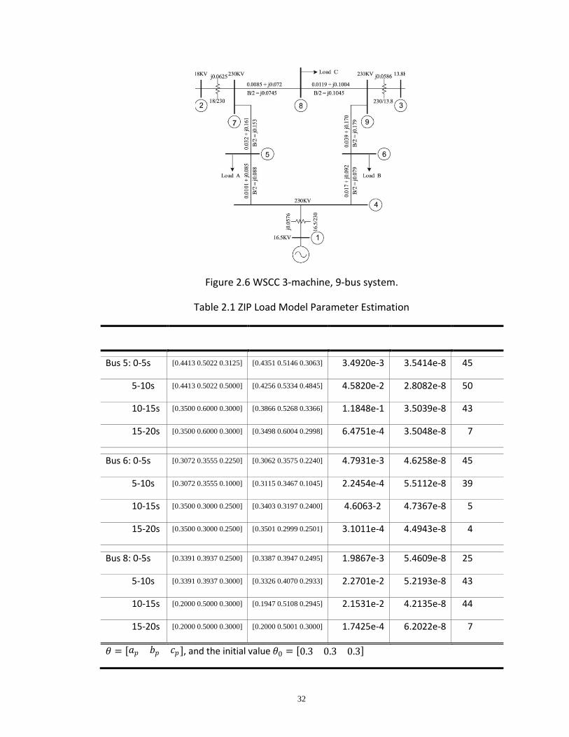
Figure 2.6 WSCC 3-machine, 9-bus system. ..................................................................... 32
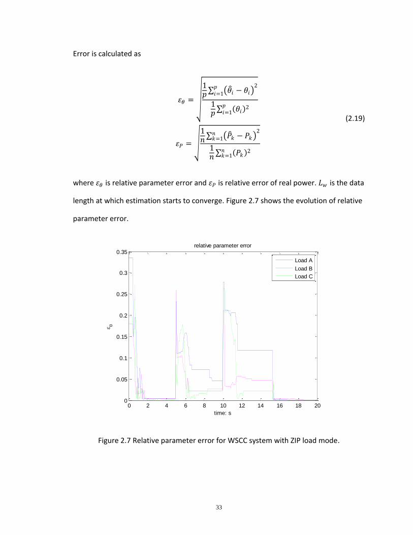
Figure 2.7 Relative parameter error for WSCC system with ZIP load mode. ................... 33
Figure 2.8 Relative parameter error for WSCC system with exponential load model. .... 34
Figure 2.9 GNLD and nonparametric model simulated results compared with
measurement. .................................................................................................. 36
Figure 2.10 30-bus, 9-machine system. ............................................................................ 37
Figure 2.11 Relative parameter error of ZIP load model using noisy data. ...................... 42
Figure 2.12 Relative parameter error of exponential load model using noisy data. ....... 43
Figure 2.13 Relative parameter error of GNLD load model using noisy data. ................. 43
Figure 3.1 The illustration of particle filters algorithm. .................................................... 56
Figure 3.2 Two-vortex single-tracer. ................................................................................. 60
Figure 3.3 Two-vortex two-tracer.. ................................................................................... 61
Figure 3.4 Full state estimation using PFs and EKF. .......................................................... 66
Figure 3.5 Full state estimation using PFs and EKF with large 𝑣. ..................................... 67
Figure 3.6 The PSS/E results and PFs estimation results of machine angle and speed
of machine 1. ................................................................................................... 69
Figure 3.7 The PSS/E results and EKF estimation results of machine angle and speed
of machine 1. ................................................................................................... 70
Figure 3.8 The evolution of 𝑝(𝑥𝑘|𝑦1: 𝑘) according to PFs. .............................................. 71
Figure 3.9 Estimated inertia H. ......................................................................................... 72
Figure 3.10 Estimated variation of system noise/uncertainties. ...................................... 73
Figure 3.11 Estimated relative speed with unknown system variation. .......................... 74
Figure 3.12 Fixed lag smoother 𝐿 = 10. ........................................................................... 76
Figure 4.1 The topology of study and external areas. ...................................................... 93
Figure 4.2 Eigenvalue distributions of original system and reduced system via BT. ........ 95
Figure 4.3 System frequency response of original system and reduced system using
BT. .................................................................................................................... 96
viii
Figure 4.4 Hankel singular values via balanced realization. ............................................. 96
Figure 4.5 One tie-line case. ............................................................................................. 97
Figure 4.6 Eigenvalue distributions of unreduced / reduced system via BT and Krylov
subspace........................................................................................................... 99
Figure 4.7 System frequency responses. .......................................................................... 99
Figure 4.8 System frequency responses. ........................................................................ 100
Figure 4.9 One tie-line case. ........................................................................................... 101
Figure 4.10 Sensitivity analysis of machine angles. ........................................................ 104
Figure 4.11 Sensitivity analysis of bus voltages. ............................................................. 105
Figure 4.12 Singular value frequency response. ............................................................. 106
Figure 4.13 Three tie-line case. ....................................................................................... 107
ix
LIST OF TABLES
Table 2.1 ZIP Load Model Parameter Estimation ............................................................. 32
Table 2.2 Exponential Load Model Parameter Estimation ............................................... 34
Table 2.3 GNLD Model Parameter Estimation .................................................................. 35
Table 2.4 GNLD Model Parameter Estimation .................................................................. 36
Table 2.5 Exponential Load Model Parameter Estimation ............................................... 37
Table 2.6 ZIP Load Model Parameter Estimation ............................................................. 38
Table 3.1 Relative Error of PFs, EKF and other Algorithms ............................................... 77

1
CHAPTER 1
INTRODUCTION
World Energy Outlook 2008: In our Reference Scenario, which assumes no new
government policies beyond those already adopted by mid-2008,world primary energy
demand expands by 45% between 2006 and 2030. ... Electricity demand is increasing
much more rapidly than overall energy use and is likely to almost double from 2004 to
2030. ... Modern renewable technologies grow most rapidly, overtaking gas soon after
2010 to become the second-largest source of electricity behind coal. [1]
With worldwide rapid industrial growth, the demand for electric power is dramatically
rising daily. To reduce the increasing disparity between energy demand and supply, new
energy resources have been investigated and new technologies implemented. The
steadily expanding load demand, together with the changes in technology, require the
present electric power system to operate with narrow stability and security margins,
while maintaining high reliability. Thus, the power system is increasingly stressed. There
is an acute need to better understand the dynamic nature of power system behavior
and to have good knowledge of the dynamic states of the system in order to be
prepared for critical situations as they arise.
To fulfill this need, this dissertation focuses on three areas using dynamic data available
from phasor measurement units in real time: developing more accurate dynamic load
models by updating variable parameters, estimating states and parameters of
synchronous machines and identifying the influences from the disturbances or

2
uncertainties within power system, and addressing the computational issues which arise
during power system analysis.
1.1 Motivation
POWER SYSTEM FACT: Today’s electricity system is 99.97 percent reliable, yet still allows
for power outages and interruptions that cost Americans at least $150 billion each year
— about $500 for every man, woman and child. [2]
“Our century-old power grid is the largest interconnected machine on Earth, so
massively complex and inextricably linked to human involvement and endeavor that it
has alternately (and appropriately) been called an ecosystem. It consists of more than
9,200 electric generating units with more than 1,000,000 megawatts of generating
capacity connected to more than 300,000 miles of transmission lines….
In celebrating the beginning of the 21st century, the National Academy of Engineering
set about identifying the single most important engineering achievement of the 20th
century. The Academy compiled an estimable list of twenty accomplishments which
have affected virtually everyone in the developed world. The internet took thirteenth
place on this list, and ‘highways’ eleventh. Sitting at the top of the list was electrification
as made possible by the grid, ‘the most significant engineering achievement of the 20th
Century.’…
Yet, the grid is now struggling to keep up with the rapidly increasing demand. From
1988-98, U.S. electricity demand rose by nearly 30 percent, while the transmission
network’s capacity grew by only 15%.... There have been five massive blackouts over the
past 40 years, three of which have occurred in the past nine years. More blackouts and

3
brownouts are occurring due to the slow response times of mechanical switches, a lack
of automated analytics, and ‘poor visibility’ – a ‘lack of situational awareness’ on the
part of grid operators. This issue of blackouts has far broader implications than simply
waiting for the lights to come on. Imagine plant production stopped, perishable food
spoiling, traffic lights dark, and credit card transactions rendered inoperable. Such are
the effects of even a short regional blackout.” [2]
Power system engineers are using advanced technologies to transform the grid into an
intelligent system and thereby improve power grid visibility. Real-time information
feedback is essential. Hence, engineers need access to the real-time dynamic
phenomena. Power system control centers should become information technology
centers, where the continuous monitoring and control of different signals and
components will result in powerful diagnosis of the system [3], —and therefore in high
reliability.
Phasor measurement units (PMU) use synchronization signals from the GPS satellite
system to directly measure dynamic power system phenomena and provide phase
angles and magnitudes of voltages and currents [4]. This innovative measurement tool
can capture both the slow variation of voltages and currents, and the underlying
oscillations in a power system. Moreover, the GPS time-synchronized PMU sample at
about 30-60 per second, and are accurate to 1 ms at any location on earth. Traditional
remote terminal units (RTU) can only achieve a sample rate of less than 1 Hz locally with
no global synchronization.
The deployment of PMU enables the direct observation of system oscillations, including
under system disturbances. By trying to simulate these events, we can learn a great deal

4
about the models of major system components, and correct them as needed until the
simulations and observed phenomena match well [4].
The commercial manufacture of PMU allows power system engineers to explore
potential applications such as state estimation, instability prediction, fault
detection/location, control improvement, etc. This dissertation focuses on the
application of real-time identification of system dynamics.
Developing and maintaining simulation-based planning models that accurately
represent the behavior of the system is obviously critical to better plan and operate the
transmission systems. There is no question that the dynamic properties of power system
loads have a major impact on system stability. And system planners must also be able to
validate the load and generator in order to reliably plan their systems in the most
economical manner. Real-time identification of power system load and generator
models will give power system engineers a more visible power system. Hence it will
supply more valuable information for analyzing, planning and operating the power grid.
1.2 Load Modeling
There is no question that load representation has a significant impact on system stability
analysis [5], [6]. Loads, in combination with other dynamics, are among the main
contributors of low voltage conditions, voltage instability and even collapse in the
power system. And it is becoming more evident that load model uncertainty is the
largest single source of simulation inaccuracy for planning and operations. As transfer
limits of the power flow are determined by such study, load model accuracy is critical
for maintaining the secure and economic operation of the power system.

5
Current load models applied to system planning in utilities, based on research
conducted in the 1970s and 1980s, may not be able to account for the continuous
changes in the electricity industry which have forced changes in the transmission
system, such that power systems now operate closer to their limits. While scientifically
accurate and detailed models have been proposed for generators, lines, transformers
and control devices, the same has not occurred for load models because of the random
nature of a load composition.
There are two main approaches to developing load models: the physical component
based approach and the measurement data based approach. We can determine the
aggregate load model parameters if the parameters of all separate loads are well
known. However, with the large number and types of loads connected at the
transmission system level, such a physical component based approach to aggregate
separate loads is numerically impractical. Therefore, in the absence of the precise
information, we choose the measurement data based approach to obtain a reliable load
model by implementing system identification techniques. This approach includes
developing models with appropriate parameters and validating models with real-world
response. Field measurements of voltage variations and the associated real and reactive
power responses are required for the development and validation of the load models.
Computer programming is needed to provide models that capture system dynamics and
represent loads against actual system load behavior.
The load models also need to be updated in a timely manner to assure the best
performance since the loads are actually evolving with time. While quite a few papers
discuss how to express the load model [7 - 9], there have been few attempts to develop
a dynamic load model with variable parameters and to detect the parameter changes

6
while there is no huge disturbance and, hence, no big voltage variations. The final report
on the August 14, 2003, blackout also indicated that one cause of the huge blackout was
that the Midwest Independent System Operator (MISO) was using non-real-time data to
support real-time operations [10].
As such, one focus of this work is to identify and update the load models with real-time
data, so that a more adequate and timely understanding of power system loads can be
achieved.
1.3 Nonlinear Filtering
The commonly used power system models are deterministic. They might not catch up
with underlying disturbances and oscillations, and hence might not be able to support
good decision making in various situations. Furthermore, for some devices, such as
generators, the original parameters from installation might be out of date. Parameter
validation should be performed regularly to insure the necessary adjustments, so that
reliable planning can be made in the most economical manner.
We study the advanced filtering concepts and technologies, such as extended Kalman
filters (EKF) and particle filters (PFs), to adopt the disturbances and uncertainties in the
system models, and apply them to the real-time identification of system models.
We consider the situation where the nature of the monitored environment will be
captured by a Markovian state-space model that involves potentially nonlinear
dynamics, nonlinear observations, system uncertainties and observation noise. In a
nonlinear environment, particle methods, which include sequential Monte Carlo and
interacting particle filters, are very useful. Our goal is to perform sequential estimation

7
of the current system state/parameter at multiple sensor nodes in the power network
system.
Two models are required In order to analyze and make inferences about the dynamic
power system: First, a model describing the evolution of the state with time (the system
model) and, second, a model relating the noisy measurements to the state (the
measurement model). We will assume that the system is subject to random noise in a
probabilistic form, so that it is more realistic. The probabilistic state-space formulation
and the requirement for the updating of information on receipt of new measurements
are ideally suited for the Bayesian approach.
In the Bayesian approach we follow, an estimate is required every time a measurement
is received. This can be obtained through a recursive filtering approach, which means
that received data can be processed sequentially rather than as a batch so that it is
neither necessary to store the complete data set nor to reprocess existing data if a new
measurement becomes available. Such a filter essentially consists of two stages:
prediction and update. The prediction stage uses the system model to predict the state
probability density function (pdf) forward from one measurement time to the next.
Since the state is usually subject to unknown disturbances (modeled as random noise),
prediction generally translates, deforms, and spreads the state pdf. The update
operation uses the latest measurement to modify the prediction pdf. This is achieved
using Bayes theorem, which is the mechanism for updating knowledge about the target
state in the light of extra information from new data.
Two specific filtering algorithms are studied, extended Kalman filter (EKF) and particle
filters (PFs). Extended Kalman filter utilizes the first term in a Taylor expansion of the
8
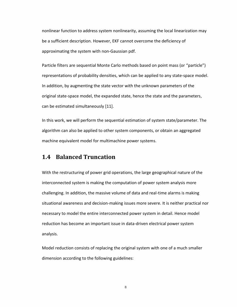
nonlinear function to address system nonlinearity, assuming the local linearization may
be a sufficient description. However, EKF cannot overcome the deficiency of
approximating the system with non-Gaussian pdf.
Particle filters are sequential Monte Carlo methods based on point mass (or “particle”)
representations of probability densities, which can be applied to any state-space model.
In addition, by augmenting the state vector with the unknown parameters of the
original state-space model, the expanded state, hence the state and the parameters,
can be estimated simultaneously [11].
In this work, we will perform the sequential estimation of system state/parameter. The
algorithm can also be applied to other system components, or obtain an aggregated
machine equivalent model for multimachine power systems.
1.4 Balanced Truncation
With the restructuring of power grid operations, the large geographical nature of the
interconnected system is making the computation of power system analysis more
challenging. In addition, the massive volume of data and real-time alarms is making
situational awareness and decision-making issues more severe. It is neither practical nor
necessary to model the entire interconnected power system in detail. Hence model
reduction has become an important issue in data-driven electrical power system
analysis.
Model reduction consists of replacing the original system with one of a much smaller
dimension according to the following guidelines:

9
• The reduced system must be an accurate representation of the original one for
the analysis performed.
• The cost of generating the reduced model must be much smaller than the cost of
performing the analysis using the original model.
We partition interconnected power systems into two areas in system analysis: the study
area and the external area [12]. The study area contains the variables of interest, and
therefore it is modeled in detail. The external area is important only as insofar as it
influences the analysis in the study area and therefore is represented by a linear model
which can be further replaced by a reduced-order system. Then we focus on the model
reduction for the external area.
The model reduction methods for power system analysis can be roughly classified into
two categories, engineering methods and mathematical methods. Research in this area
dates back to the 1970s, and most work has focused on the engineering method side,
coherency identification. Mathematical methods have gained more attention recently,
but most of them work with state matrices. Since we are only interested in the
influences of the external area, the input-output behavior is more important than the
external area itself. Based on this, we study the balanced truncation method for model
reduction in power systems.
Balanced truncation is a known projection model reduction method which delivers high
quality reduced models [13]. It has been applied in spacecraft modeling, control system
design, and other areas of large dimension modeling. Balanced truncation is based on
introducing a special joint measure of controllability and observability for every vector
in the state space of an LTI system. Then, the reduced model is obtained by removing
10
those components of the state vector which have the lowest importance factor in terms
of this measure.
In this work, the framework for using the balanced truncation method in power systems
is provided. Additionally, the sensitivity analysis is performed to further include the
consideration for the nonlinear nature of power systems.
1.5 Contributions
The main contributions of the work included in this thesis can be summarized as follows:
Analysis of the impact of load-voltage characteristics in the planning and
operation of power systems.
Procedures for load identification and algorithms for load parameter estimation.
Criteria for load parameter estimatability from noisy data.
Algorithms of particle filtering for power systems.
Augmented particle filters for parameter estimation.
Model reduction of power systems with balanced truncation.
Sensitivity analysis to update the system model.
1.6 Thesis Overview
The thesis is organized as follows.
In Chapter 2, an analysis of the load-voltage characteristic is provided. Then different
types of loads are introduced. Procedures for load identification are proposed. The
Levernberg-Marquardt algorithm is studied for load parameter estimation. The criteria
for parameter estimatability from noisy data are then developed. In Chapter 3,
11
nonlinear filtering algorithms such as extended Kalman filters and particle filters are
studied. Then, such nonlinear filtering methods are applied in power system analysis. In
Chapter 4, we study model reduction using the balanced truncation method. The results
are compared with those of the Krylov subspace method. Sensitivity analysis to update
the system model because of system nonlinearity is also performed. In Chapter 5, the
main conclusions of the work are summarized, and ideas for further work are presented.
1.7 References
[1] WEO, World Energy Outlook - 2008. London: International Energy Agency, 2008.
[2] Litos Strategic Communication, The Smart Grid: An Introduction. Prepared for the
U. S. Department of Energy.
[3] C. A. Canizares, "Voltage stability assessment: Concepts, practices and tools," IEEE-
PES Power Systems Stability Subcommittee, Special Publication SP101PSS, August
2002.
[4] G. Phadke, "Synchronized phasor measurements in power systems," IEEE Computer
Applications in Power, vol. 6, no. 2, pp. 10-15, April 1993.
[5] C. W. Taylor, Power System Voltage Stability. New York, NY: McGraw-Hill, 1994.
[6] IEEE Task Force on Load Representation for Dynamic Performance, "Load
representation for dynamic performance analysis," IEEE Transactions on Power
Systems, vol. 8, no. 2, pp. 472-482, May 1993.
[7] D. J. Hill, "Nonlinear dynamic load models with recovery for voltage stability
studies," IEEE Transactions on Power Systems, vol. 8, no. 1, pp. 166-176, Feb. 1993.
[8] W. W. Price et al., "Load modeling for power flow and transient stability computer
studies," IEEE Transactions on Power Systems, vol. 3, no. 1, pp. 180-187, Feb. 1988.
[9] W. Xu and Y. Mansour, "Voltage stability analysis using generic dynamic load
models," IEEE Transactions on Power Systems, vol. 9, no. 1, pp. 479-493, May 1994.

12
[10] U.S.-Canada Power System Outage Task Force, "Final report on the August 14, 2003
blackout in the United States and Canada," April 2004.
[11] G. Kitagawa, "A self-organizing state-space mode," Journal of American Statistical
Association, vol. 93, no. 443, pp. 1203-1215, September 1998.
[12] Electric Power Research Institute, "Development of dynamic equivalents for
transient stability studies," Palo Alto, CA, Tech. Rep. EL-456, Project 763, 1977.
[13] S. Gugercin and A. C. Antoulas, "Survey of model reduction by balanced truncation
and some new results," International Journal of Control, vol. 77, no. 8, pp. 748-766,
May 2004.

13
CHAPTER 2
LOAD MODELING
2.1 Introduction
Load model is a mathematical representation related to the measured voltage and/or
frequency at a bus, and the power consumed by the load, active and reactive. Accurate
load models are required to correctly understand the potential for voltage collapse and
system oscillations following system disturbances. Transmission power flow limits are
determined from studies of these conditions. Load modeling is essential to provide
secure and economic planning and operation of a power system. There is increasing
interest in load modeling in recent years: it has become a new research area in power
system stability. Equation Chapter 2 Section 1
Various static and dynamic models based on mathematical and physical representations
have been studied to describe the overall load characteristics [1].
Classical static load models have been used in production-grade load flow programs for
years. Common static load models for active and reactive power are expressed in a
polynomial or an exponential form, and can include, if necessary, a frequency
dependence term [2]. But in recent years, several studies have shown the critical effect
of load representation in voltage stability studies [1], [2], and therefore the idea of using
static load models in stability analysis is changing in favor of dynamic load models.

14
Even though power system load has gained more attention, it is still considered one of
the most uncertain and difficult components to model due to the large number of
diverse load components, variable composition with time of day and week, weather and
through time, and also because of lack of precise information on the composition of the
load.
With the availability of phasor measurement units (PMU), we now can get access to the
dynamic phenomena of electric power systems and form an improved load
representation. In addition, the combination of the accurate load models with real-time
updated parameters will help us decrease the uncertainty margin, resulting in a reliable
and economic operation of the power system.
The rest of this chapter is organized as follows. Different load representations are
introduced first. The impacts of load characteristics on voltage stability are then studied.
The load identification process and algorithm are proposed. Simulation results are given.
And the criteria are developed to study the parameter estimatability from noisy data.
2.2 Load Models
Load models are classified mainly as static or dynamic. A static load model is not
dependent on time, and therefore it describes the relation of the active and reactive
power at any time with the voltage and/or frequency at the same instant of time. In
contrast, a dynamic load model expresses this relation at any instant of time as a
function of the voltage and/or frequency time history, including, typically, the present
moment.
We can summarize the relation as:
15
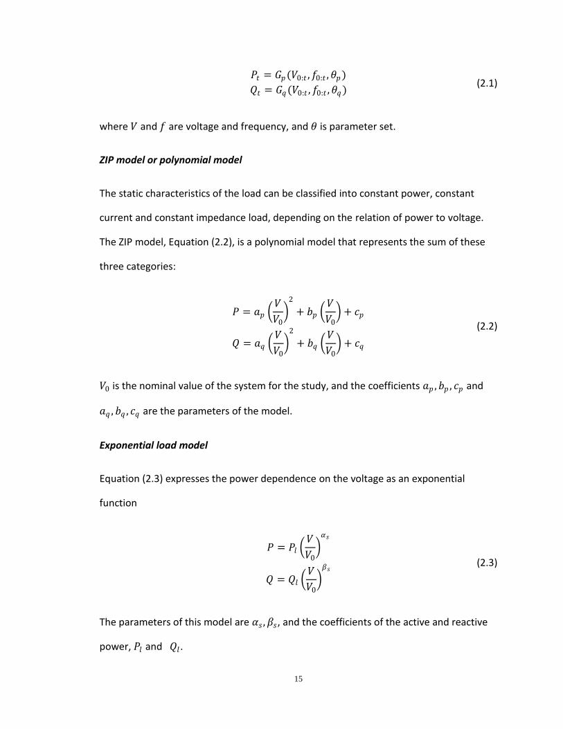
𝑃𝑡 = 𝐺𝑝(𝑉0:𝑡 , 𝑓0:𝑡 , 𝜃𝑝)
𝑄𝑡 = 𝐺𝑞(𝑉0:𝑡 , 𝑓0:𝑡 , 𝜃𝑞) (2.1)
where 𝑉 and 𝑓 are voltage and frequency, and 𝜃 is parameter set.
ZIP model or polynomial model
The static characteristics of the load can be classified into constant power, constant
current and constant impedance load, depending on the relation of power to voltage.
The ZIP model, Equation (2.2), is a polynomial model that represents the sum of these
three categories:
𝑃 = 𝑎𝑝 𝑉
𝑉0
2
+ 𝑏𝑝 𝑉
𝑉0 + 𝑐𝑝
𝑄 = 𝑎𝑞 𝑉
𝑉0
2
+ 𝑏𝑞 𝑉
𝑉0 + 𝑐𝑞
(2.2)
𝑉0 is the nominal value of the system for the study, and the coefficients 𝑎𝑝 , 𝑏𝑝 , 𝑐𝑝 and
𝑎𝑞 , 𝑏𝑞 , 𝑐𝑞 are the parameters of the model.
Exponential load model
Equation (2.3) expresses the power dependence on the voltage as an exponential
function
𝑃 = 𝑃𝑙 𝑉
𝑉0 𝛼𝑠
𝑄 = 𝑄𝑙 𝑉
𝑉0 𝛽𝑠
(2.3)
The parameters of this model are 𝛼𝑠 , 𝛽𝑠, and the coefficients of the active and reactive
power, 𝑃𝑙 and 𝑄𝑙 .

16
Generic nonlinear dynamic load models
When the traditional static load models are not sufficient to represent the behavior of
the load, the alternative dynamic load models are necessary.
In 1993, the popular dynamic load model was proposed by Hill in [3], which captures the
usual nonlinear steady state behavior plus load recovery and overshoot. Other similar
dynamic load models [4] have been developed based on the same philosophy, steady
state behavior plus transients. Such load models are called generic nonlinear dynamic
(GNLD) load models. We will adopt the exponential recovery dynamic load model from
Hill’s work [3]. The mathematical expression of the model is
𝑃𝑑 = 𝑃0 𝑉
𝑉0 𝛼𝑡
+ 𝑧𝑝
𝑇𝑝𝑧𝑝 = −𝑧𝑝 + 𝑃0 𝑉
𝑉0 𝛼𝑠
− 𝑃0 𝑉
𝑉0 𝛼𝑡
𝑄𝑑 = 𝑄0 𝑉
𝑉0 𝛽𝑡
+ 𝑧𝑞
𝑇𝑞𝑧𝑞 = −𝑧𝑞 + 𝑄0 𝑉
𝑉0 𝛽𝑠
− 𝑄0 𝑉
𝑉0 𝛽𝑡
(2.4)
where 𝑧𝑝 and 𝑧𝑞 are the corresponding recovery load states for real and reactive
power, respectively; 𝑇𝑝 and 𝑇𝑞 are the load recovery time constants; 𝑃𝑑 and 𝑄𝑑 are the
real and reactive load power demands; and 𝑃0 , 𝑄0, and 𝑉0 denote nominal real, reactive
power, and voltage, respectively. The exponents 𝛼𝑠, 𝛼𝑡 , 𝛽𝑠, and 𝛽𝑡 stand for steady state
and transient load-voltage dependences.
Equation (2.4) is the additive aggregate dynamic load model. Similarly, there is
multiplicative aggregate dynamic load model:

17
𝑃𝑑 = 𝑧𝑝𝑃0 𝑉
𝑉0 𝛼𝑡
𝑇𝑝𝑧𝑝 = 𝑉
𝑉0 𝛼𝑠
− 𝑧𝑝 𝑉
𝑉0 𝛼𝑡
𝑄𝑑 = 𝑧𝑞𝑄0 𝑉
𝑉0 𝛽𝑡
𝑇𝑞𝑧𝑞 = 𝑉
𝑉0 𝛽𝑠
− 𝑧𝑞 𝑉
𝑉0 𝛽𝑡
(2.5)
Nonparametric load models
The nonparametric load models may consider the load or individual load components as
a “black box,” and transfer functions can be used to represent the load dynamics due to
voltage variations.
The first-order linear dynamic load models can be characterized as functions of the
change in system voltage
∆𝑃𝑙 =𝑘𝑝𝑣 + 𝑇𝑝𝑣𝑠
𝑇1𝑝𝑠 + 1∆𝑉
∆𝑄𝑙 =𝑘𝑞𝑣 + 𝑇𝑞𝑣𝑠
𝑇1𝑞𝑠 + 1∆𝑉
(2.6)
where 𝑘 and 𝑇 are the load parameters for real or reactive power as functions of
voltage depending on the subscript and 𝑇1 is the time constant of the load.
Or we can use the difference equation:

18
∆𝑃𝑙 𝑘 = 𝑎𝑖𝑗 ∆𝑃𝑙 𝑘 − 𝑖 𝑗
𝑛𝑝
𝑖=1
𝑚𝑝
𝑗 =1
+ 𝑏𝑖𝑗 ∆𝑉 𝑘 − 𝑖 𝑗
𝑛𝑝𝑣
𝑖=1
𝑚𝑝𝑣
𝑗=1
∆𝑄𝑙 𝑘 = 𝑐𝑖𝑗 ∆𝑄𝑙 𝑘 − 𝑖 𝑗
𝑛𝑞
𝑖=1
𝑚𝑞
𝑗 =1
+ 𝑑𝑖𝑗 ∆𝑉 𝑘 − 𝑖 𝑗
𝑛𝑞𝑣
𝑖=1
𝑚𝑣𝑞
𝑗 =1
(2.7)
Equation (2.7) will be used to estimate load parameters in Section 2.5.
Frequency dependent load models
Sometimes, the load model can also include frequency dependence, by multiplying the
equations by the factor of the form:
1 + 𝐾𝑝 𝑓 − 𝑓0
and 1 + 𝐾𝑞 𝑓 − 𝑓0 (2.8)
where 𝑓0 and 𝑓 are the nominal frequency and the frequency of the bus voltage, and
the parameters 𝐾𝑝 and 𝐾𝑞 represent the frequency sensitivity of the model.
Augmented load models
Load models are not necessarily either static or dynamic. In fact, they are more likely to
be a combination of both. We can use static models, either ZIP or exponential,
augmented with dynamic ones to represent the loads
𝑃 = 𝑃𝑠 + 𝑃𝑑
𝑄 = 𝑄𝑠 + 𝑄𝑑 (2.9)
where 𝑃𝑠 , 𝑄𝑠 are from Equation (2.2) or (2.3), and 𝑃𝑑 , 𝑄𝑑 are from Equation (2.4) or (2.5).
GNLD also belongs to this category.

19
Other widely used dynamic load models include the industrial load models (IM) using
first or third or even higher order approximation for motors, or a combination of static
and IM, such as [5], [6], [7]. A good summary of research and development in the area
of load modeling can be found in [2].
2.3 Influence of Load Characteristics on Voltage Stability
As mentioned, load characteristics are critical to the study of voltage stability. In this
section, we will briefly explain the effect of load representation on voltage stability.
Voltage stability is defined as the ability of a power system to maintain steady
acceptable voltage at all buses in the system at normal operating conditions, and after
being subjected to a disturbance. Voltage collapse follows voltage instability. According
to IEEE definitions [8], “voltage collapse is the process by which the sequence of events
accompanying voltage instability leads to a blackout or abnormally low voltages in a
significant part of the power system.”
The determination of the maximum amount of power that a system can supply to a load
will make it possible to define the voltage stability margins of the system, and how they
can be affected by various events. The PV curve [1] corresponds to the graphical
representation of the power-voltage function at the load bus. The PV curves are
characterized by a parabolic shape, which describes how a specific power can be
transmitted at two different voltage levels, high and low voltage. The desired working
points are those at high voltage, in order to minimize power transmission losses due to
high currents at low voltages. The vertex of the parabola determines the maximum
power that can be transmitted by the system, and it is often called the point of
maximum loadability or point of collapse.

20
The Western System Coordinating Council (WSCC) system (Figure 2.6 on page 32) has
been used to illustrate the PV curve. Figure 2.1 shows the PV curve of load A on bus 5.
When the point of collapse is reached, the system becomes unstable, and the voltage
starts decreasing quickly since the reactive support of the system under these heavily
loaded conditions is not enough.
Figure 2.1 PV curve.
The load representation will affect the location of the operating point in the PV curves,
leading the system closer to or farther away from the maximum loadability point. An
optimistic design may lead the system to voltage collapse under severe conditions,
while a conservative design will reduce the transfer capacity due to larger security
margins.
We use general static models in exponential form to illustrate such effect.
0 1 2 3 4 5 60
0.2
0.4
0.6
0.8
1
P Load: p.u.
V L
oad:
p.u
. Maximum Loadability, Pmax
21
𝑃 = 𝑃𝑙 𝑉
𝑉0 𝛼𝑠
𝑄 = 𝑄𝑙 𝑉
𝑉0 𝛽𝑠
(2.10)
We can get constant power, constant current, or constant impedence load model by
setting 𝛼𝑠 equal to 0, 1, or 2. The exponent 𝛼𝑠 might also have negative values due to
the long-term dynamic restoration of the load, and the effect of discrete tap changers
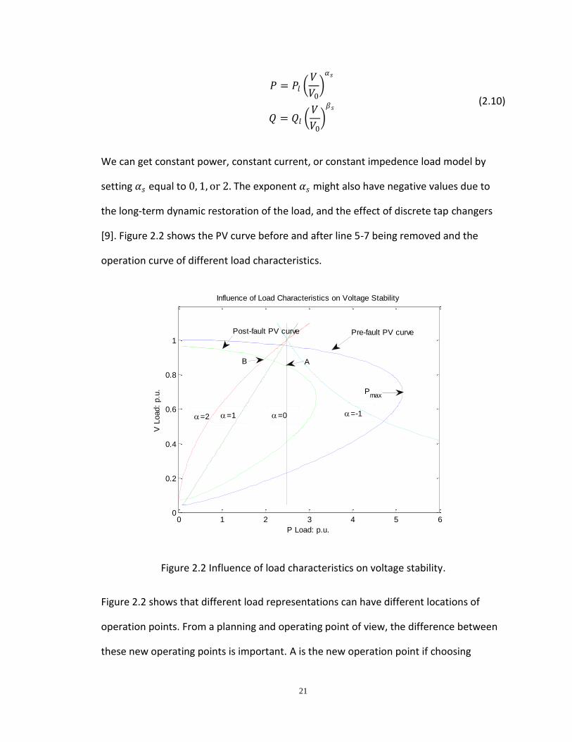
[9]. Figure 2.2 shows the PV curve before and after line 5-7 being removed and the
operation curve of different load characteristics.
Figure 2.2 Influence of load characteristics on voltage stability.
Figure 2.2 shows that different load representations can have different locations of
operation points. From a planning and operating point of view, the difference between
these new operating points is important. A is the new operation point if choosing
0 1 2 3 4 5 60
0.2
0.4
0.6
0.8
1
P Load: p.u.
V L
oad:
p.u
.
Influence of Load Characteristics on Voltage Stability
Pmax
=-1=0=1=2
Pre-fault PV curvePost-fault PV curve
AB

22
constant power as the load model, and B is the one if choosing constant impedance as
the load model. If the actual load is constant impedance, by assuming a constant power
characteristic, the impact of the load in the system is overemphasized and the
theoretical transfer capacity is reduced, which in the end leads to a poor utilization of
the system. If the actual load is constant power, by assuming a constant impedance
characteristic, then the impact of the load in the system is under-emphasized and the
system is operating closer to the collapse point. The figure also shows that, if 𝛼𝑠 = −1,
then the system is unstable.
In order to analyze the effect of power loads on voltage stability, it is also necessary to
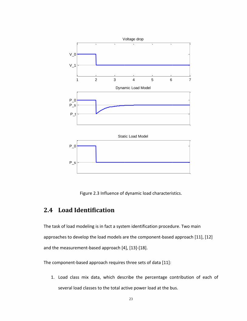
study the influence of dynamic characteristics of the load. Figure 2.3 shows an ideal
voltage step change and the corresponding load responses from dynamic and static load
representations. We can see that there is a recovery time from the transient state to
the steady state for dynamic load representation. For electric heating, which shows a
thermostatic effect, the resulting operating point of the dynamic model is more critical
than the one predicted by the static model [10].
23
Figure 2.3 Influence of dynamic load characteristics.
2.4 Load Identification
The task of load modeling is in fact a system identification procedure. Two main
approaches to develop the load models are the component-based approach [11], [12]
and the measurement-based approach [4], [13]-[18].
The component-based approach requires three sets of data [11]:
1. Load class mix data, which describe the percentage contribution of each of
several load classes to the total active power load at the bus.
1 2 3 4 5 6 7
V_1
V_0
Voltage drop
P_t
P_s
P_0
Dynamic Load Model
P_s
P_0
Static Load Model

24
2. Load composition data, which describe the percentage contribution of each of
several load components to the active power consumption of a particular load
class.
3. Load characteristics data, which describe the electrical characteristics — e.g.,
power factor, voltage and frequency sensitivity — of each of the load
components.
For an area whose load composition and characteristics will not vary widely, the
component-based approach has the advantage of not requiring system measurements
and therefore being more readily put into use.
For most systems, the loads are actually changing dramatically over time. Also, it is
unrealistic to obtain all detailed individual components necessary for building the load
model, not to mention the fact that it is impossible to update the data simultaneously.
This work focuses on load modeling from a measurement-based approach.
The measurement-based approach uses system identification techniques to estimate a
proper model and its parameters. The process of system identification involves finding a
suitable model structure (mathematical model) and appropriate parameters for this
structure that can replicate the dynamic response between change in voltage and
corresponding changes in active and reactive powers.
The overall procedure (shown in Figure 2.4) used in this work is summarized as follows:
1 Data Acquisition
o Acquire measurement data (V, I, P, Q)
2 Voltage Detection
3 System Identification and Load Modeling

25
o Determine load structures to be used
o Identify which parameters can be estimated reliably from the available
measurements
o Estimate parameters using a suitable method and an estimation criterion
o Validate the derived model
4 System Accepted
Our work is mainly in Step 2 and Step 3.
Figure 2.4 Load modeling procedure flow chart.
2.4.1 Voltage variation detection
Since the data acquired contain mixed information, a procedure for detecting voltage
variation must be applied before the start of load modeling. We compare the incoming
preprocessed data; if the voltage variation is in order of or greater than 1%, we open a
new window and start the model identification process. The voltage variation can be
detected from three sources: system disturbance excitation, load variation and bad
data. The first two provide valuable information for load model identification.
Data Acquisition
• Data Recording
• Data Pre-processing (Data convention and selection)
• Voltage Variation Detection
System Identification and Load Modeling
• Determine the load model structure
• Estimate Load Parameters- Apply Parameter Estimation Techniques and Criteria- Estimate the parameters for the proposed model
• Validate Load Model and Parameters- Compare the predicted output values (P, Q) with measurement- Estimate the errors in the estimated parameters and model
• If unsatisfactory, try another model structure and repeat the process until “satisfactory” load model is obtained
System Acceptance
• Accepted System

26
2.4.2 Load structure selection
Before engaging the complicated calculation, first we want to select a proper load
structure to start with. Such selection could be based on the knowledge and experience
of the system under study.
P-V relation
If no other information is available, we can identify whether static or dynamic load
models are more suitable to describe the load with no complicated calculation or
estimation, but, rather by inspecting the P-V relation1 and the first derivative of load
power w. r. t. voltage (Figure 2.5).
The first derivative of load power w. r. t. voltage for static load models is
𝑑𝑃
𝑑𝑉𝑠𝑡𝑎𝑡𝑖𝑐 =
2𝑎𝑝
𝑉
𝑉0 + 𝑏𝑝 ZIP Model
𝑃0
𝑉𝛼𝑠−1
𝑉0𝛼𝑠
Exponential Model
(2.11)
The first derivative of load power w. r. t. voltage for dynamic load models is
𝑑𝑃
𝑑𝑉𝑑𝑦𝑎𝑛𝑚𝑖𝑐=
𝑃
𝑉 =
−𝑧𝑝 + 𝑃0 𝑉𝑉0
𝛼𝑠
− 𝑃0 𝑉𝑉0
𝛼𝑡
𝑉 for additive GDNL
(2.12)
Within normal operation range, the relative deviation of 𝑑𝑃
𝑑𝑉𝑠𝑡𝑎𝑡𝑖𝑐 is small, while
𝑑𝑃
𝑑𝑉𝑑𝑦𝑛𝑎𝑚𝑖𝑐 will have infinite peak when 𝑉 is 0. Hence, the P-V relation of static loads will
1 The P-V curve mentioned here is not for power transfer and voltage stability study, but purely to illustrate the
relationship between P and V, which are captured by PMUs during the normal operations.
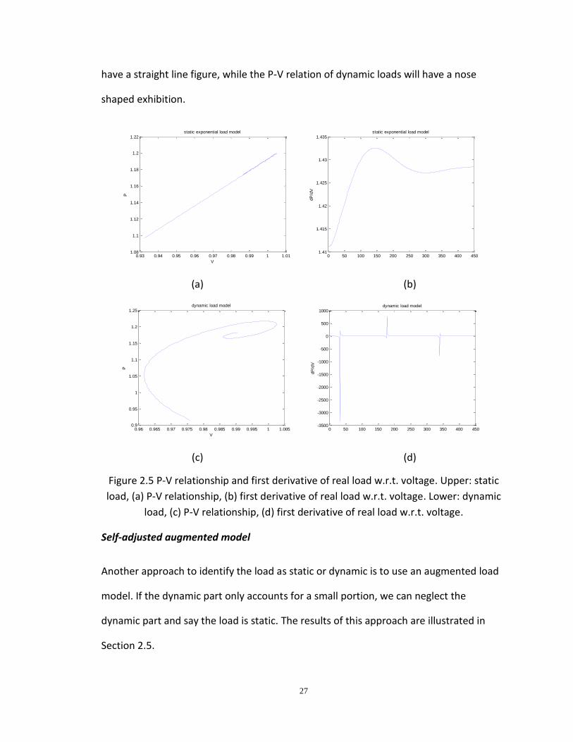
27
have a straight line figure, while the P-V relation of dynamic loads will have a nose
shaped exhibition.
(a) (b)
(c) (d)
Figure 2.5 P-V relationship and first derivative of real load w.r.t. voltage. Upper: static
load, (a) P-V relationship, (b) first derivative of real load w.r.t. voltage. Lower: dynamic
load, (c) P-V relationship, (d) first derivative of real load w.r.t. voltage.
Self-adjusted augmented model
Another approach to identify the load as static or dynamic is to use an augmented load
model. If the dynamic part only accounts for a small portion, we can neglect the
dynamic part and say the load is static. The results of this approach are illustrated in
Section 2.5.
0.93 0.94 0.95 0.96 0.97 0.98 0.99 1 1.011.08
1.1
1.12
1.14
1.16
1.18
1.2
1.22static exponential load model
P
V
0 50 100 150 200 250 300 350 400 4501.41
1.415
1.42
1.425
1.43
1.435
dP
/dV
static exponential load model
0.96 0.965 0.97 0.975 0.98 0.985 0.99 0.995 1 1.0050.9
0.95
1
1.05
1.1
1.15
1.2
1.25
V
P
dynamic load model
0 50 100 150 200 250 300 350 400 450-3500
-3000
-2500
-2000
-1500
-1000
-500
0
500
1000dynamic load model
dP
/dV
28
2.4.3 Parameter estimation
After determining the right category of load model, the second step is to estimate
parameters. That is, find a set of parameters for which the simulated results from
proposed model best fit the measurement. In other words, find the optimal estimation
of the parameters that minimizes the sum of the squares of the errors defined by
𝑓 𝜃 = 𝑦 𝑘 𝜃 −𝑦𝑘 2
𝑘
(2.13)
where 𝑦𝑘 is the actual (observed) power at time 𝑘, which would be the real and reactive
power, 𝑦 𝑘 𝜃 is the given model prediction, and 𝜃 is the parameter vector that needs to
be estimated.
Accompanying the development of different load models, various parameter estimation
algorithms have been applied in identifying the models. Least-square methods are one
of the most popular [5], [13], [15], [16]. Recently, more complex estimation techniques
have been adopted in load model parameter estimation, such as generic algorithms
(GAs) [17], simulated annealing (SA) [18], and artificial neural networks (ANNs) [14].
The algorithm we choose here is the Levenberg-Marquardt algorithm (LMA) [19], [20].
LMA is known for its robustness. Like other numeric minimization algorithms, LMA is an
iterative procedure. In each iteration step, the parameter vector 𝜃 is replaced by a new
estimate 𝜃 + ∆𝜃. To determine ∆𝜃, the function 𝑓(𝜃) is expanded around 𝜃 by the
Taylor series, and neglecting the higher order terms in the Taylor expansion beyond
quadratics, we can get
29
∆𝜃 = − 𝑓 ′ ′ 𝜃 −1𝑓 ′ 𝜃 (2.14)
This coincides with one step of the Newton-Raphson method for solving the necessary
condition for a local minimum. It can be rewritten as
𝐴 𝜃 ∆𝜃 = −𝐽 𝜃 (2.15)
Since the data are around the normal operational point, it is very likely that 𝐴 is close to
singular in our case. LMA is a robust algorithm to avoid the singularity problem.
The LMA modifies Equation (2.15) by introducing the matrix 𝐴 with entries
𝑎 𝑗𝑗 = 1 + 𝛾 𝑎𝑗𝑗
𝑎 𝑗𝑘 = 𝑎𝑗𝑘 , 𝑗 ≠ 𝑘 (2.16)
where 𝛾 is some positive parameter. At time step 𝑘, Equation (2.15) becomes
𝐴 𝜃𝑘 𝜃𝑘+1 − 𝜃𝑘 = −𝐽 𝜃𝑘 (2.17)
For large 𝛾, the matrix 𝐴 will become diagonally dominant, which will avoid the
singularity of 𝐴. As 𝛾 approaches zero, Equation (2.17) will turn into the Newton-
Raphson method. Depending on the residue of 𝑓, change the damping parameter by
factor 𝛾𝜈𝑘 , for some 𝑘 ∈ 𝑍.
The basic LMA is summarized as follows:
Step 1: Set 𝑘 = 0. Choose an initial guess 𝜃0, 𝛾 and factor 𝜈.
Step 2: Solve Equation (2.16) to obtain 𝜃𝑘+1.
Step 3: Compare 𝑓 𝜃𝑘+1 and 𝑓 𝜃𝑘 .
30
If 𝑓 𝜃𝑘+1 > 𝑓 𝜃𝑘 , reject 𝜃𝑘+1, replace 𝛾 by 𝛾𝜈, and repeat step 2.
If 𝑓 𝜃𝑘+1 < 𝑓 𝜃𝑘 , accept 𝜃𝑘+1, replace 𝛾 by 𝛾/𝜈, set 𝑘 = 𝑘 + 1 and repeat
step 2.
Step 4: Terminate the iteration when the termination criteria are met.
2.4.4 Load model validation
The derived parameter values need to be validated for their expected performance. The
validation includes two steps: check the model quality on the identification data, and
validate the model on a different set of measurement data.
For the first step, the load model output (response) is simulated and then compared
with the measured output using the obtained parameter values. We evaluate the
performance of the developed load model using the following relative error
휀𝑦 =
1𝑛
𝑦 𝑘 − 𝑦𝑘 2𝑛𝑘=1
1𝑛
𝑦𝑘 2𝑛𝑘=1
(2.18)
where 𝑦𝑘 and 𝑦 𝑘 denote the measured and simulated (real or reactive) power,
respectively. If 휀𝑦 is less than the desired threshold, say 1%, the dynamic load model is
said to be acceptable.
If the performance achieved on the identification data is acceptable, the second step is
to validate the model on a different set of measurement data, since parameter variance
error could not be detected from the training data set. We need to choose identification
data and measurement data carefully because the parameter is always time-varying.

31
In the next section, we apply the automatic identification procedure discussed above.
2.5 Simulation Results
In this section, several cases with different load models are simulated using the
automatic identification procedure. The voltage variation is detected to start the
estimation process. Load type is determined both by inspecting the P-V relation and by
using the self-augmented model. LMA is used to estimate model parameters. The
identification data window is 3 s or until converge, whichever is larger. And the
estimation results are validated by using the data after that until another voltage
variation is detected.
Case 1: 3-Machine, 9-Bus System with PSS/E Static Load Model
The popular Western System Coordinating Council (WSCC) 3-machine, 9-bus system is
used in the case study. Figure 2.6 is the one-line diagram of the system. PSS/E [21] was
used to generate the data as a realistic simulation. The output of PSS/E was then used as
the measurements for load identification. We use GENTRA for the machine model, IEEE1
for the exciter and TGOV1 for the governor. Both the static ZIP load model and static
exponential load model are used in PSS/E simulation. Since we want to check the
algorithm feasibility for updating time-variant parameters within normal operation
conditions, we change the load parameters at times 5 s and 10 s, followed by a self-
clearing fault at 15 s. The GNLD model is used, and if the dynamic term is detected to be
negligible, it will self-adjust to static load model. Table 2.1 shows the estimation results
for the ZIP load model.
32
Figure 2.6 WSCC 3-machine, 9-bus system.
Table 2.1 ZIP Load Model Parameter Estimation
Actual 𝜽 Estimated 𝜽 𝜺𝜽 𝜺𝑷 𝑳𝒘
Bus 5: 0-5s [0.4413 0.5022 0.3125] [0.4351 0.5146 0.3063] 3.4920e-3 3.5414e-8 45
5-10s [0.4413 0.5022 0.5000] [0.4256 0.5334 0.4845] 4.5820e-2 2.8082e-8 50
10-15s [0.3500 0.6000 0.3000] [0.3866 0.5268 0.3366] 1.1848e-1 3.5039e-8 43
15-20s [0.3500 0.6000 0.3000] [0.3498 0.6004 0.2998] 6.4751e-4 3.5048e-8 7
Bus 6: 0-5s [0.3072 0.3555 0.2250] [0.3062 0.3575 0.2240] 4.7931e-3 4.6258e-8 45
5-10s [0.3072 0.3555 0.1000] [0.3115 0.3467 0.1045] 2.2454e-4 5.5112e-8 39
10-15s [0.3500 0.3000 0.2500] [0.3403 0.3197 0.2400] 4.6063-2 4.7367e-8 5
15-20s [0.3500 0.3000 0.2500] [0.3501 0.2999 0.2501] 3.1011e-4 4.4943e-8 4
Bus 8: 0-5s [0.3391 0.3937 0.2500] [0.3387 0.3947 0.2495] 1.9867e-3 5.4609e-8 25
5-10s [0.3391 0.3937 0.3000] [0.3326 0.4070 0.2933] 2.2701e-2 5.2193e-8 43
10-15s [0.2000 0.5000 0.3000] [0.1947 0.5108 0.2945] 2.1531e-2 4.2135e-8 44
15-20s [0.2000 0.5000 0.3000] [0.2000 0.5001 0.3000] 1.7425e-4 6.2022e-8 7
𝜃 = 𝑎𝑝 𝑏𝑝 𝑐𝑝 , and the initial value 𝜃0 = 0.3 0.3 0.3
33
Error is calculated as
휀𝜃 =
1𝑝
𝜃 𝑖 − 𝜃𝑖 2𝑝
𝑖=1
1𝑝
𝜃𝑖 2𝑝𝑖=1
휀𝑃 =
1𝑛
𝑃 𝑘 − 𝑃𝑘 2𝑛
𝑘=1
1𝑛
𝑃𝑘 2𝑛𝑘=1
(2.19)
where 휀𝜃 is relative parameter error and 휀𝑃 is relative error of real power. 𝐿𝑤 is the data
length at which estimation starts to converge. Figure 2.7 shows the evolution of relative
parameter error.
Figure 2.7 Relative parameter error for WSCC system with ZIP load mode.
0 2 4 6 8 10 12 14 16 18 200
0.05
0.1
0.15
0.2
0.25
0.3
0.35
time: s
relative parameter error
Load A
Load B
Load C
34
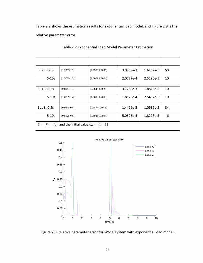
Table 2.2 shows the estimation results for exponential load model, and Figure 2.8 is the
relative parameter error.
Table 2.2 Exponential Load Model Parameter Estimation
Actual 𝜽 Estimated 𝜽 𝜺𝜽 𝜺𝑷 𝑳𝒘
Bus 5: 0-5s [1.2565 1.2] [1.2566 1.2053] 3.0868e-3 1.6202e-5 50
5-10s [1.5079 1.2] [1.5079 1.2004] 2.0789e-4 2.5290e-5 10
Bus 6: 0-5s [0.8844 1.4] [0.8843 1.4028] 3.7736e-3 1.8826e-5 10
5-10s [1.0809 1.4] [1.0808 1.4003] 1.8176e-4 2.5407e-5 10
Bus 8: 0-5s [0.9875 0.8] [0.9874 0.8018] 1.4426e-3 1.0686e-5 34
5-10s [0.5925 0.8] [0.5925 0.7994] 5.0596e-4 1.8298e-5 6
𝜃 = 𝑃𝑙 𝛼𝑠 , and the initial value 𝜃0 = 1 1
Figure 2.8 Relative parameter error for WSCC system with exponential load model.
0 1 2 3 4 5 6 7 8 9 100
0.05
0.1
0.15
0.2
0.25
0.3
0.35
0.4
0.45
0.5
time: s
relative parameter error
Load A
Load B
Load C
35
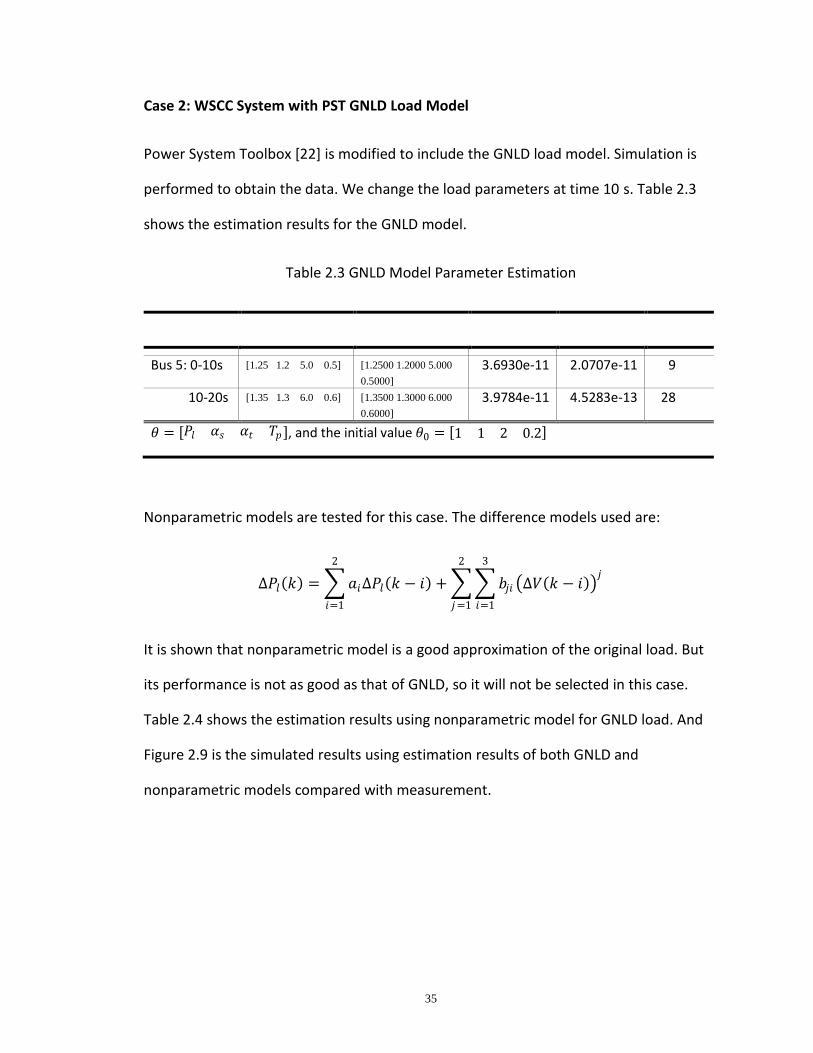
Case 2: WSCC System with PST GNLD Load Model
Power System Toolbox [22] is modified to include the GNLD load model. Simulation is
performed to obtain the data. We change the load parameters at time 10 s. Table 2.3
shows the estimation results for the GNLD model.
Table 2.3 GNLD Model Parameter Estimation
Actual 𝜽 Estimated 𝜽 𝜺𝜽 𝜺𝑷 𝑳𝒘
Bus 5: 0-10s [1.25 1.2 5.0 0.5] [1.2500 1.2000 5.000
0.5000]
3.6930e-11 2.0707e-11 9
10-20s [1.35 1.3 6.0 0.6] [1.3500 1.3000 6.000
0.6000]
3.9784e-11 4.5283e-13 28
𝜃 = 𝑃𝑙 𝛼𝑠 𝛼𝑡 𝑇𝑝 , and the initial value 𝜃0 = 1 1 2 0.2
Nonparametric models are tested for this case. The difference models used are:
∆𝑃𝑙 𝑘 = 𝑎𝑖∆𝑃𝑙 𝑘 − 𝑖
2
𝑖=1
+ 𝑏𝑗𝑖 ∆𝑉 𝑘 − 𝑖 𝑗
3
𝑖=1
2
𝑗=1
It is shown that nonparametric model is a good approximation of the original load. But
its performance is not as good as that of GNLD, so it will not be selected in this case.
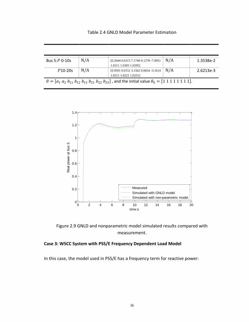
Table 2.4 shows the estimation results using nonparametric model for GNLD load. And
Figure 2.9 is the simulated results using estimation results of both GNLD and
nonparametric models compared with measurement.
36
Table 2.4 GNLD Model Parameter Estimation
Actual 𝜽 Estimated 𝜽 𝜺𝜽 𝜺𝑷
Bus 5:𝑃 0-10s N/A [0.2644 0.6315 7.1740 0.1278 -7.0951
1.0311 1.0303 1.0295]
N/A 1.3538e-2
𝑃10-20s N/A [0.9591 0.0151 3.1562 0.0654 -3.1614
1.0211 1.0221 1.0231]
N/A 2.6213e-3
𝜃 = 𝑎1 𝑎2 𝑏11 𝑏12 𝑏13 𝑏21 𝑏22 𝑏23 , and the initial value 𝜃0 = 1 1 1 1 1 1 1 1 .
Figure 2.9 GNLD and nonparametric model simulated results compared with
measurement.
Case 3: WSCC System with PSS/E Frequency Dependent Load Model
In this case, the model used in PSS/E has a frequency term for reactive power:
0 2 4 6 8 10 12 14 16 18 200
0.2
0.4
0.6
0.8
1
1.2
1.4
time:s
Real pow
er
at
bus 5
Measured
Simulated with GNLD model
Simulated with non-parametric model

37
𝑃 = 𝑃𝑙 𝑉
𝑉0 𝛼𝑠
𝑄 = 𝑄𝑙 𝑉
𝑉0 𝛽𝑠
× 1 + 𝐾𝑄 𝑓 − 𝑓0
(2.20)
Table 2.5 shows the estimation results.
Table 2.5 Exponential Load Model Parameter Estimation
Actual 𝜽 Estimated 𝜽 𝜺𝜽 𝜺𝑷 𝑳𝒘
Bus 5: 𝑃 [1.25 1.2 0.0] [1.2500 1.2005 0.0087] 4.9658e-3 5.2693e-3 11
𝑄 [0.50 1.6 5.0] [0.5000 1.6006 5.0123] 2.3094e-3 7.0196e-3 11
𝜃 = 𝑃𝑙 𝛼𝑠 𝐾𝑃 or 𝑄𝑙 𝛽𝑠 𝐾𝑄 , and the initial value 𝜃0 = 1 1 0
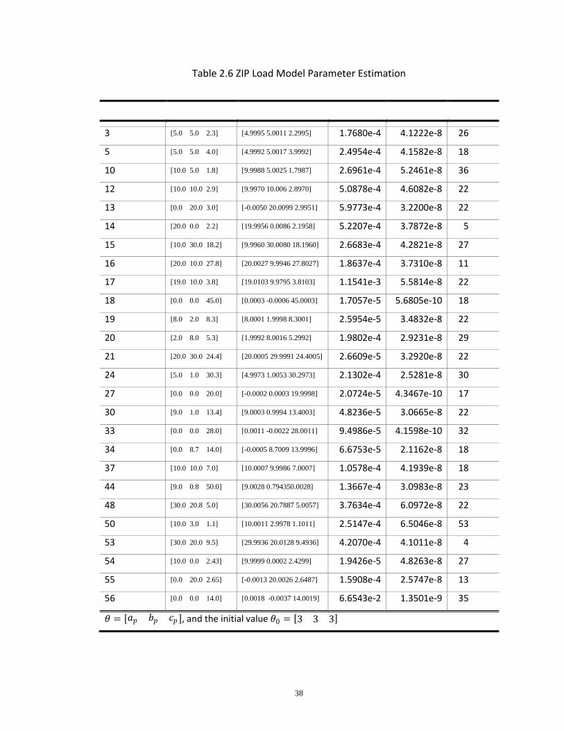
Case 4: 30-Bus System using PowerWorld with Static Load Model
The 30-bus, 9-machine system with ZIP load model is used in PowerWorld. Figure 2.10
shows the one-line diagram of the system. Table 2.6 is the estimation results.
Figure 2.10 30-bus, 9-machine system.
38
Table 2.6 ZIP Load Model Parameter Estimation
Bus
Number
Actual 𝜽 Estimated 𝜽 𝜺𝜽 𝜺𝑷 𝑳𝒘
3 [5.0 5.0 2.3] [4.9995 5.0011 2.2995] 1.7680e-4 4.1222e-8 26
5 [5.0 5.0 4.0] [4.9992 5.0017 3.9992] 2.4954e-4 4.1582e-8 18
10 [10.0 5.0 1.8] [9.9988 5.0025 1.7987] 2.6961e-4 5.2461e-8 36
12 [10.0 10.0 2.9] [9.9970 10.006 2.8970] 5.0878e-4 4.6082e-8 22
13 [0.0 20.0 3.0] [-0.0050 20.0099 2.9951] 5.9773e-4 3.2200e-8 22
14 [20.0 0.0 2.2] [19.9956 0.0086 2.1958] 5.2207e-4 3.7872e-8 5
15 [10.0 30.0 18.2] [9.9960 30.0080 18.1960] 2.6683e-4 4.2821e-8 27
16 [20.0 10.0 27.8] [20.0027 9.9946 27.8027] 1.8637e-4 3.7310e-8 11
17 [19.0 10.0 3.8] [19.0103 9.9795 3.8103] 1.1541e-3 5.5814e-8 22
18 [0.0 0.0 45.0] [0.0003 -0.0006 45.0003] 1.7057e-5 5.6805e-10 18
19 [8.0 2.0 8.3] [8.0001 1.9998 8.3001] 2.5954e-5 3.4832e-8 22
20 [2.0 8.0 5.3] [1.9992 8.0016 5.2992] 1.9802e-4 2.9231e-8 29
21 [20.0 30.0 24.4] [20.0005 29.9991 24.4005] 2.6609e-5 3.2920e-8 22
24 [5.0 1.0 30.3] [4.9973 1.0053 30.2973] 2.1302e-4 2.5281e-8 30
27 [0.0 0.0 20.0] [-0.0002 0.0003 19.9998] 2.0724e-5 4.3467e-10 17
30 [9.0 1.0 13.4] [9.0003 0.9994 13.4003] 4.8236e-5 3.0665e-8 22
33 [0.0 0.0 28.0] [0.0011 -0.0022 28.0011] 9.4986e-5 4.1598e-10 32
34 [0.0 8.7 14.0] [-0.0005 8.7009 13.9996] 6.6753e-5 2.1162e-8 18
37 [10.0 10.0 7.0] [10.0007 9.9986 7.0007] 1.0578e-4 4.1939e-8 18
44 [9.0 0.8 50.0] [9.0028 0.794350.0028] 1.3667e-4 3.0983e-8 23
48 [30.0 20.8 5.0] [30.0056 20.7887 5.0057] 3.7634e-4 6.0972e-8 22
50 [10.0 3.0 1.1] [10.0011 2.9978 1.1011] 2.5147e-4 6.5046e-8 53
53 [30.0 20.0 9.5] [29.9936 20.0128 9.4936] 4.2070e-4 4.1011e-8 4
54 [10.0 0.0 2.43] [9.9999 0.0002 2.4299] 1.9426e-5 4.8263e-8 27
55 [0.0 20.0 2.65] [-0.0013 20.0026 2.6487] 1.5908e-4 2.5747e-8 13
56 [0.0 0.0 14.0] [0.0018 -0.0037 14.0019] 6.6543e-2 1.3501e-9 35
𝜃 = 𝑎𝑝 𝑏𝑝 𝑐𝑝 , and the initial value 𝜃0 = 3 3 3

39
2.6 Parameter Estimatability
Measurement data contain noise for most cases. If the noise exceeds the dynamic
variations, then we cannot obtain reliable parameter estimation results from the
contaminated data. In this section, we develop the criteria to decide whether the
information contained in a data set is enough to estimate parameters.
2.6.1 Sensitivity matrix
The sensitivity matrix [23] plays an important role in deciding the parameter
identifiability. The mathematical representation of load model is
𝑃𝑡 = 𝐺𝑝(𝑉0:𝑡 , 𝑓0:𝑡 , 𝜃𝑝)
𝑄𝑡 = 𝐺𝑞(𝑉0:𝑡 , 𝑓0:𝑡 , 𝜃𝑞) (2.21)
For now, we only consider real power
𝑃 = 𝐺(𝑉, 𝑓, 𝜃) (2.22)
Assuming the initial guess is 𝜃0, observation 𝑃 𝑘 can be calculated. Now we linearize the
observations around the initial estimates:
𝑃𝑘 = 𝐺𝑘0 +
𝜕𝐺𝑘0
𝜕𝜃𝑗∆𝜃𝑗
𝑝
𝑗 =1
+ 𝑒𝑗 (2.23)
The squared deviation over the simulated data set is

40
𝑓 𝜃 = 𝑃𝑘 − 𝐺𝑘0 −
𝜕𝐺𝑘0
𝜕𝜃𝑗∆𝜃𝑗
𝑝
𝑗 =1
2𝑛
𝑘=1
(2.24)
We let 𝑧𝑘 = 𝑃𝑘 − 𝐺𝑘0, ∆𝜃 = ( ∆𝜃 1, … , ∆𝜃 𝑝) be the least-square estimates of ∆𝜃, and 𝑔
be the sensitivity matrix:
𝑔 =
𝜕𝐺10
𝜕𝜃1⋯
𝜕𝐺10
𝜕𝜃𝑝
⋮ ⋱ ⋮𝜕𝐺𝑛
0
𝜕𝜃1⋯
𝜕𝐺𝑛0
𝜕𝜃𝑝
(2.25)
The normal equations for the estimates of ∆𝜃 are given by
𝑔′𝑔∆𝜃 = 𝑔′𝑧 = 0 (2.26)
If the determinant of 𝑔′𝑔 ≠ 0, then the model is structurally locally identifiable. For the
insensible parameters, the corresponding columns have only zero entries.
If the relevant 𝑔′𝑔 matrix is near singular, i.e., the determinant of 𝑔′𝑔 is close to zero,
then the parameter set has poor estimatability.
2.6.2 Trajectory sensitivity
For the dynamic load model, the derivation of the sensitivity matrix is not
straightforward. We use trajectory sensitivity analysis [24], [25] to calculate 𝑔. The
dynamic load model can be written as
𝑥 = 𝑓(𝑥, 𝜃)𝑃 = (𝑥, 𝜃)
(2.27)

41
Trajectory sensitivity analysis studies the variations of the system variables with respect
to the small variations in initial conditions and parameters [26].
The differential equation with respect to the initial conditions and parameters yields
𝑥 𝜃 = 𝑓𝑥𝑥𝜃 + 𝑓𝜃𝐼𝑔 = 𝑥𝑥𝜃 + 𝜃
(2.28)
where 𝑓𝑥 , 𝑓𝜃 , 𝑥 and 𝜃 are time-varying matrices and are evaluated along the system
trajectories.
2.6.3 Estimatability criteria
As mentioned in 2.6.1, if the determinant of the sensitivity matrix is near singular, the
parameter is hard to estimate. LMA in Section 2.4.3 modifies the diagonal entries of 𝑔′𝑔
to avoid the singularity. Such modification can walk into the subspace of solutions for
nonidentifiable parameters and stop when the termination criteria are satisfied. In such
poorly estimatable cases, the estimation results generally yield a small overall sum of
squares, indicating one is getting a good fit to the observations and, coupled with that, a
very large standard deviation of the estimates of some parameters, for estimates from
several data sets. This indicates that some of the parameters are unidentifiable, or
identifiable but very poorly estimatable.
Besides the sensitivity matrix, signal-to-noise ratio (SNR) is also a good measurement for
noisy data. The data would be corrupted if the noise exceeded the variation, even with a
large SNR. So instead, we replace signal power with variation power, and define
42
𝑆𝑁𝑅𝑚 =𝑃𝑠𝑖𝑔𝑛𝑎𝑙 −𝑚𝑒𝑎𝑛 (𝑠𝑖𝑔𝑛𝑎𝑙 )
𝑃𝑛𝑜𝑖𝑠𝑒 (2.29)
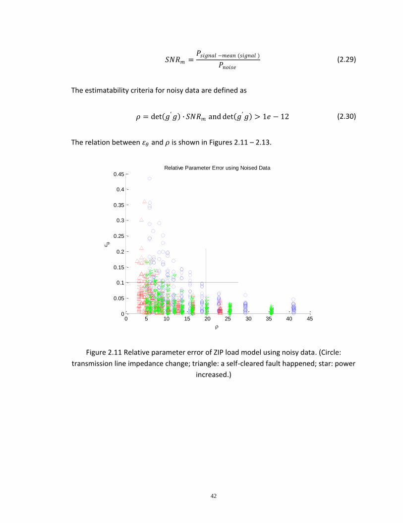
The estimatability criteria for noisy data are defined as
𝜌 = det 𝑔′𝑔 ∙ 𝑆𝑁𝑅𝑚 and det 𝑔′𝑔 > 1𝑒 − 12 (2.30)
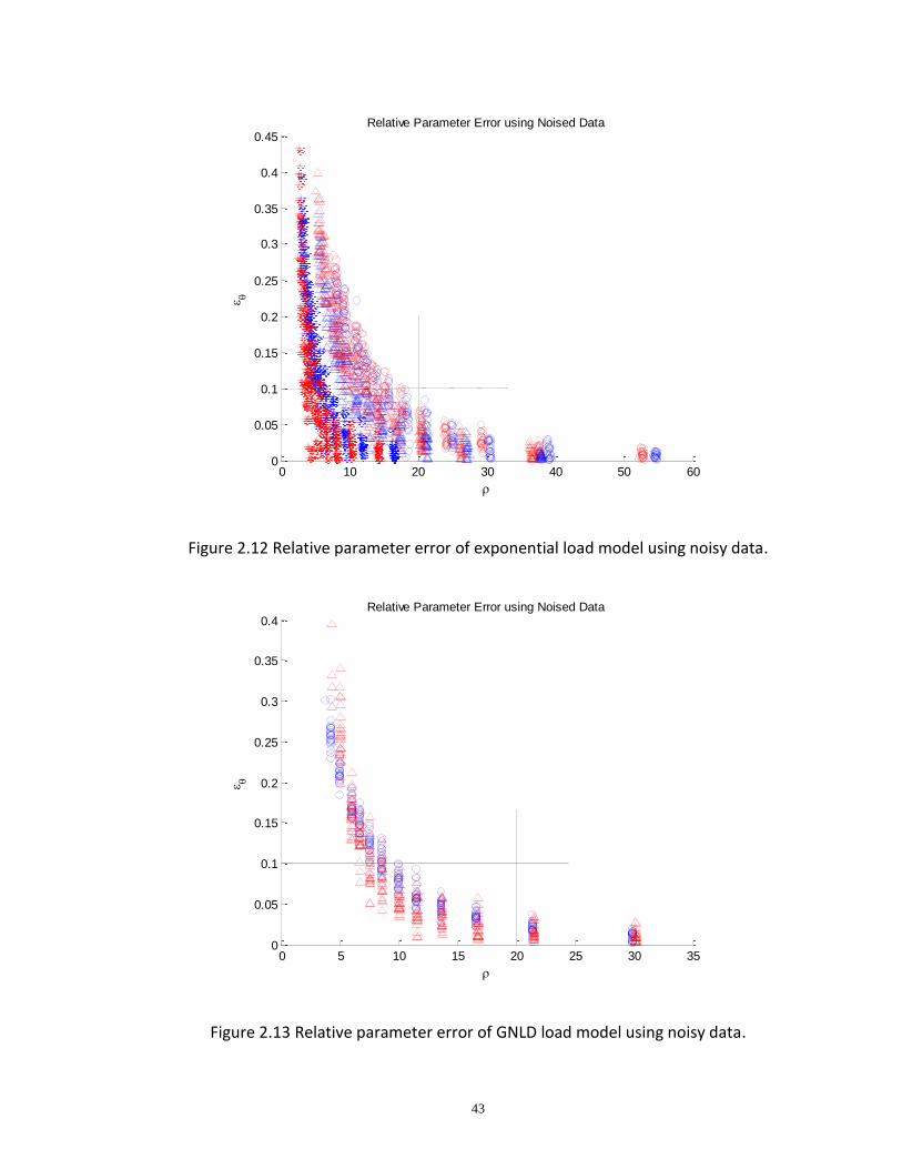
The relation between 휀𝜃 and 𝜌 is shown in Figures 2.11 – 2.13.
Figure 2.11 Relative parameter error of ZIP load model using noisy data. (Circle:
transmission line impedance change; triangle: a self-cleared fault happened; star: power
increased.)
0 5 10 15 20 25 30 35 40 450
0.05
0.1
0.15
0.2
0.25
0.3
0.35
0.4
0.45Relative Parameter Error using Noised Data
43
Figure 2.12 Relative parameter error of exponential load model using noisy data.
Figure 2.13 Relative parameter error of GNLD load model using noisy data.
0 10 20 30 40 50 600
0.05
0.1
0.15
0.2
0.25
0.3
0.35
0.4
0.45
Relative Parameter Error using Noised Data
0 5 10 15 20 25 30 350
0.05
0.1
0.15
0.2
0.25
0.3
0.35
0.4
Relative Parameter Error using Noised Data

44
The simulation results of different models and different cases are consistent. When
𝜌 > 20, 휀𝜃 < 0.1. Larger 𝜌 can be chosen if higher accuracy is desired.
The multiplication of sensitivity matrix determinant and modified SNR is a good term to
judge identifiability of the parameter.
2.7 Conclusion
In this chapter, we have shown that load representations have an influence on voltage
stability study. A wrongly selected model will either cause a stability problem or reduce
the transfer capacity. The overall identification procedure for load modeling is proposed
and discussed. The proposed procedure can capture the voltage variation and so can
update load parameters in real time. Simulation results prove that LMA is robust and
stable. It is suitable for load parameter estimation from operation data with no big
disturbances. Parameter estimatability with noisy data is an important practical issue.
The criteria to decide the estimatability are developed and tested.
Other related readings are [27]-[39].
2.8 References
[1] C. W. Taylor, Power System Voltage Stability. New York, NY: McGraw-Hill, 1994.
[2] IEEE Task Force on Load Representation for Dynamic Performance, "Load
representation for dynamic performance analysis," IEEE Transactions on Power
Systems, vol. 8, no. 2, pp. 472-482, May 1993.
[3] D. J. Hill, "Nonlinear dynamic load models with recovery for voltage stability
studies," IEEE Transactions on Power Systems, vol. 8, no. 1, pp. 166-176, Feb. 1993.
[4] W. Xu and Y. Mansour, "Voltage stability analysis using generic dynamic load

45
models," IEEE Transactions on Power Systems, vol. 9, no. 1, pp. 479-493, May 1994.
[5] C.-J. Lin et al., "Dynamic load models in power systems using the measurement
approach," IEEE Transactions on Power Systems, vol. 8, no. 1, pp. 309-315, Feb.
1993.
[6] CIGRE Task Force 38-02-10, "Modeling of voltage collapse including dynamic
phenomena," CIGRE Brochure No. 75, 1993.
[7] M. A. Merkel and A. M. Miri, "Modelling of industrial loads for voltage stability
studies in power systems," in Canadian Conference on Electrical and Computer
Engineering, 2001, May 2001, pp. 0881-0886.
[8] P. Kundur et al., "Definition and classification of power system stability IEEE/CIGRE
joint task force on stability terms and definitions," IEEE Transactions on Power
Systems, vol. 19, no. 3, pp. 1387-1401, Aug. 2004.
[9] I. R. Navarro, "Dynamic power system load: Estimation of parameters from
operational data," Ph.D. dissertation, Lund University, Lund, Sweden, 2005.
[10] C. A. Canizares, "Voltage stability assessment: Concepts, practices and tools," IEEE-
PES Power Systems Stability Subcommittee, Special Publication SP101PSS , August
2002.
[11] W. W. Price et al., "Load modeling for power flow and transient stability computer
studies," IEEE Transactions on Power Systems, vol. 3, no. 1, pp. 180-187, Feb. 1988.
[12] S. Ihara, M. Tani, and K. Tomiyama, "Residential load characteristics observed at
KEPCO power system," IEEE Transactions on Power Systems, vol. 9, no. 2, pp. 1092-
1101, May 1994.
[13] A. Borghetti, R. Caldon, A. Mari, and C. A. Nucci, "On dynamic load models for
voltage stability studies," IEEE Transactions on Power Systems, vol. 12, no. 1, pp.
293-303, Feb. 1997.
[14] A. P. Alves da Silva, C. Ferreira, A. C. Zambroni de Souza, and G. Lambert-Torres, "A
new constructive ANN and its application to electric load representation," IEEE
Transactions on Power Systems, vol. 12, no. 4, pp. 1596-1575, Nov. 1997.
[15] B.-K. Choi, H.-D. Chiang, Y.-T. Chen, D.-H. Huang, and M. G. Lauby, "Development of
46
composite load models of power systems using on-line measurement data," Journal
of Electrical Engineering & Technology, vol. 1, no. 2, pp. 161-169, 2006.
[16] B.-K. Choi et al., "Measurement-based dynamic load models: Derivation,
comparison, and validation," IEEE Transactions on Power Systems, vol. 21, no. 3, pp.
1276-1283, Aug. 2006.
[17] P. Ju, E. Handschin, and D. Karlsson, "Nonlinear dynamic load modelling: Model and
parameter estimation," IEEE Transactions on Power Systems, vol. 11, no. 4, pp.
1689-1697, Nov. 1996.
[18] V. Knyazkin, C. A. Canizares, and L. H. Soder, "On the parameter estimation and
modeling of aggregate power system loads," IEEE Transactions on Power Systems,
vol. 19, no. 2, pp. 1023-1031, May 2004.
[19] K. Madsen, H. B. Nielsen, and O. Tingleff, Methods for Non-Linear Least Squares
Problems, 2nd ed. Lyngby, Denmark: Informatics and Mathematical Modelling
Technical University of Denmark, 2004.
[20] W. H. Press, B. P. Flannery, S. A. Teukolsky, and W. T. Vetterling, "Nonlinear
models," in Numerical Recipes in C: The Art of Scientific Computing. Cambridge, MA:
Cambridge University Press, 1992, pp. 681-689.
[21] PSS/E, Power system simulator for engineering. Schenectady, NY: Siemens - Power
Technologies Inc.
[22] J. Chow and G. Rogers, "Power Systems Toolbox." [Online]. Available:
http://www.eagle.ca/~cherry/pst.htm.
[23] A. J. Jacquez and T. Perry, "Parameter estimation: Local identifiability of
parameters," American Journal of Physiology, Endocrinology and Metabolism, vol.
258, no. 4, pp. E727-E736, April 1990.
[24] I. A. Hiskens and M. A. Pai, "Trajectory sensitivity analysis of hybrid systems," IEEE
Transactions on Circuits and Systems I: Fundamental Theory and Applications, vol.
47, no. 2, pp. 204-220, Feb. 2000.
[25] C. M. M. Ferreira, J. A. D. Pinto, and F. P. M. Barbosa, "Transient stability
assessment of an electric power system using trajectory sensitivity analysis," in
39th International Universities Power Engineering Conference, 2004, vol. 3, 2004,

47
pp. 1091-1095.
[26] M. J. Laufenberg and M. A. Pai, "A new approach to dynamic security assessment
using trajectory sensitivities," in 20th International Conference on Power Industry
Computer Application, 1997, Columbus, OH, 1997, pp. 272-277.
[27] G. Phadke, "Synchronized phasor measurements in power systems," IEEE Computer
Applications in Power, vol. 6, no. 2, pp. 10-15, April 1993.
[28] D.-Q. Ma and J. Ping, "A novel approach to dynamic load modelling," IEEE
Transactions on Power Systems, vol. 4, no. 2, pp. 396-402, May 1989.
[29] J. Y. Wen, L. Jiang, Q. H. Wu, and S. J. Cheng, "Power system load modeling by
learning based on system measurements," IEEE Transactions on Power Delivery, vol.
18, no. 2, pp. 364-371, April 2003.
[30] J. W. O'Sullivan and M. J. O'Malley, "Identification and validation of dynamic global
load model parameters for use in power system frequency simulations," IEEE
Transactions on Power Systems, vol. 11, no. 2, pp. 851-857, May 1996.
[31] H.-D. Chiang, J.-C. Wang, C.-T. Huang, Y.-T. Chen, and C.-H. Huang, "Development of
a dynamic ZIP-motor load model from on-line field measurements," International
Journal of Electrical Power & Energy Systems, vol. 19, no. 7, pp. 459-468, Oct. 1997.
[32] L. G. Dias and M. E. El-Hawary, "Nonlinear parameter estimation experiments for
static load modelling in electric power systems," IEE Proceedings on Generation,
Transmission and Distribution, vol. 136, no. 2, pp. 68-77, March 1989.
[33] J.-C. Wang et al., "Development of a frequency-dependent composite load model
using the measurement approach," IEEE Transactions on Power Systems, vol. 9, no.
3, pp. 1546-1556, Aug. 1994.
[34] I. A. Hiskens, "Nonlinear dynamic model evaluation from disturbance
measurements," IEEE Transactions on Power Systems, vol. 16, no. 4, pp. 702-710,
Nov. 2001.
[35] J. L. Huaman-Qquellon, "A variable dimension Gauss-Newton method for ill-
conditioned parameter estimation with application to a synchronous generator,"
M.S. thesis, University of Puerto Rico, Mayaguez, 2005.

48
[36] K. Tomiyama et al., "Modeling of load during and after system faults based on
actual field data," in IEEE Power Engineering Society General Meeting, 2003, vol. 3,
2003, pp. 1385-1391.
[37] S. J. Ranade, A. Ellis, and J. Mechenbier, "The development of power system load
models from measurements," in IEEE/PES Transmission and Distribution Conference
and Exposition, vol. 1, Atlanta, GA, 2001, pp. 201-206.
[38] B. C. Lesieutre, "Network and load modeling for power system dynamic analysis,"
Ph.D. dissertation, University of Illinois at Urbana-Champaign, 1993.
[39] P. W. Sauer and M. A. Pai, Power System Dynamics and Stability. Upper Saddle
River, NJ: Prentice Hall, 1998.
49
CHAPTER 3
NONLINEAR FILTERING FOR MACHINE
STATE AND PARAMETER ESTIMATION
Electrical machines are one of the most important components in power systems, and
their control is one of the greatest challenges in maintaining stable operation. The use
of machine dynamic states in advanced controls requires either direct measurement or
model-based estimation. With the emerging use of PMUs, there is an opportunity for
full dynamic state computation using the dynamic-data driven model prediction.
3.1 Introduction
A major component of any power system simulation model is the generating plant,
which comprises three major subcomponents of interest: the generator, excitation
system, and turbine/governor. Special-purpose computer programs have been
developed to simulate the dynamics of large and complex interconnected power
systems. Modern power systems are highly dependent on the proper use of dynamic
control by extensive use of computer simulation. Since the accuracy of power system
stability analysis depends on the accuracy of the models used to represent the
generating plants, the parameters used in those models could affect the calculated
margin of system stability. Use of more accurate models could result in increases in
overall power transfer capability and associated economic benefits, while inaccurate
simulation models could result in the system being allowed to operate beyond safe

50
margins. Accuracy of representation is dependent both on the structure of the
component models and the parameter values used within those models.
Since the mid 1990s, some literature has studied the “fuzzy load flow” dealing with the
uncertain but known load behavior [1], and stochastic unit commitment [2], [3], but few
attempts have been made to incorporate the noise or uncertainties into the time-
variant machine model. Equation Chapter 3 Section 1
Traditional machine models have been formulated as time-invariant systems; therefore,
they are sometimes not valid because of inaccurate parameters or constant changes in
power generation, transmission, load conditions or system configuration. Inaccuracies in
equipment modeling can be caused both by inadequate model structures and, more
often, by lack of data on equipment model parameters. “Model parameters currently
used for stability analysis are usually provided by equipment manufacturers and
calculated from design data and, in some cases, factory tests. Generally, they are not
verified by field tests. Some pieces of equipment are tuned by field personnel with
results of that initial tuning rarely incorporated into simulation models” [4]. Also,
parameters may have changed from initial values due to retuning, aging, and equipment
changes, such as generator rewinding.
One way to assure that study models are accurate is to use the dynamic data to validate
simulation models by comparing model responses with those obtained from PMU. Thus,
there is a major industry need to enhance equipment model development as well as
model parameter identification and validation [4].
Nonlinear filtering can address this need in two ways: first, by including uncertainties to
make the model time variable, and second, by using the dynamic data to estimate states
51
for control decisions — both system states for network decisions and machine states for
machine control — and to validate model parameters.
We consider the situation where the nature of the monitored environment will be
captured by a Markovian state-space model that involves potentially nonlinear
dynamics, nonlinear observations, system uncertainties and observation noises.
Assuming the system is subject to random jerks, which represent the unmodeled
dynamics of the system, as Equation (3.1), then we can apply nonlinear filtering theory
to solve the problem.
𝑥 = 𝑓 𝑥, 𝑢 + 𝑣
𝑦 = 𝑥 + 𝜆 or
𝑥𝑘+1 = 𝑓𝑘 𝑥𝑘 , 𝑢𝑘 + 𝑣𝑘
𝑦𝑘 = 𝑘 𝑥𝑘 + 𝜆𝑘 (3.1)
where 𝑥 is the system state, 𝑦 is the output, and 𝑢 is the control vector. And 𝑓𝑘 : ℝ𝑛 ×
ℝ𝑚 → ℝ𝑛 and 𝑘 : ℝ𝑛 → ℝ𝑝 are possibly nonlinear functions of the state 𝑥𝑘 . The
process and observation errors are represented by Gaussian white noise sequences 𝑣𝑘
and 𝜆𝑘 , respectively, and assumed to be independent of each other.
The sequential importance sampling (SIS) algorithm, also known as the particle filters
(PFs) method, can handle highly nonlinear dynamics in power systems [5]. PFs are the
state-space approach to modeling dynamic systems, which is convenient for handling
multivariate data and nonlinear/non-Gaussian processes [6]. In such an approach to
dynamic state estimation, one attempts to construct the posterior probability density
function of the state based on all available information, including the set of received
measurements. Details of the PF method will be explained in Section 3.2.2.
The chapter is organized as follows. Nonlinear filtering techniques, such as extended
Kalman filter and particle filters, are introduced. The feasibility of PFs is tested on vortex

52
problems. Then, we apply these nonlinear filtering techniques in machine
state/parameter estimation. The algorithms of PFs with smoother are studied. And the
conclusion is given at the end.
3.2 Extended Kalman Filter and Particle Filters
Again, the system equations are as follows:
𝑥 = 𝑓 𝑥, 𝑢 + 𝑣
𝑦 = 𝑥 + 𝜆 or
𝑥𝑘+1 = 𝑓𝑘 𝑥𝑘 , 𝑢𝑘 + 𝑣𝑘
𝑦𝑘 = 𝑘 𝑥𝑘 + 𝜆𝑘 (3.2)
where 𝑥 is the system state, 𝑦 is the output, and 𝑢 is the control vector.
Given the initial density 𝑝(𝑥0|𝑦0) ≡ 𝑝(𝑥0), we seek to find the filtered estimation of the
state, i.e., the estimation of the state 𝑥𝑘 based on the history of the past observation
𝑦1:𝑘 defined by 𝑦𝑖 : 𝑖 = 1. . . 𝑛 . The characterization of 𝑥𝑘 is given by the conditional
probability density, 𝑝 𝑥𝑘 𝑦1:𝑘 .
In the particle filters approach we follow, this can be obtained through recursive
predictions and observations. Given an initial state, a priori estimation of the state is
calculated according to Equation (3.2) in the prediction stage. After a new observation is
taken, a priori estimation is updated to become a posteriori state estimation.
The nonlinear filtering is based on the following factors:
Knowledge of the system model
The statistical description of the system and measurement noise and
uncertainties.
The initial probability distribution function (pdf), 𝑝(𝑥0|𝑦0) ≡ 𝑝(𝑥0).
53
We will discuss two important nonlinear filtering methods next, extended Kalman filter
and particle filters.
3.2.1 Extended Kalman filter (EKF)
The EKF is a suboptimal algorithm for nonlinear filtering. It assumes that 𝑣 and 𝜆 are
drawn from Gaussian distributions of known parameters. The EKF utilizes the first term
in a Taylor expansion of the nonlinear function described in Equation (3.3), assuming the
local linearization of the equations may be a sufficient description of the nonlinearity.
𝑥𝑘 = 𝐹 𝑘𝑥𝑘−1 + 𝐷𝑘𝑦𝑘−1 + 𝐵𝑘𝑢𝑘 + 𝑣𝑘−1
𝑦𝑘 = 𝐻 𝑘𝑥𝑘 + 𝜆𝑘
(3.3)
where 𝐹 𝑘 and 𝐻 𝑘 are the local linearizations of the nonlinear functions 𝑓 and , and
𝑣𝑘−1 and 𝜆𝑘 have zero mean and covariances 𝑄𝑘−1 and 𝑅𝑘 , respectively. A higher order
EKF that retains further terms in the Taylor expansion exists, but the additional
complexity prohibits its use for this problem. Based on this approximation, the posterior
pdf 𝑝(𝑥𝑘 |𝑦1:𝑘) is approximated by a Gaussian distribution.
𝑝(𝑥𝑘−1|𝑦1:𝑘−1) ≈ 𝑁(𝑥𝑘−1; 𝑚𝑘−1|𝑘−1; 𝑃𝑘−1|𝑘−1)
𝑝(x𝑘 |𝑦1:𝑘−1) ≈ 𝑁(𝑥𝑘 ; 𝑚𝑘|𝑘−1; 𝑃𝑘 |𝑘−1)
𝑝(𝑥𝑘 |𝑦1:𝑘) ≈ 𝑁(𝑥𝑘 ; 𝑚𝑘|𝑘 ; 𝑃𝑘|𝑘)
(3.4)
where
m𝑘|𝑘−1 = 𝑓𝑘 𝑚𝑘−1|𝑘−1, 𝑦𝑘 , 𝑢𝑘
𝑃𝑘|𝑘−1 = 𝑄𝑘−1 + 𝐹 𝑘𝑃𝑘−1|𝑘−1𝐹 𝑘𝑇
𝑚𝑘|𝑘 = 𝑚𝑘|𝑘−1 + 𝐾𝑘(𝑦𝑘 − 𝑘(𝑚𝑘|𝑘−1))
𝑃𝑘|𝑘 = 𝑃𝑘 |𝑘−1 − 𝐾𝑘𝐻 𝑘𝑃𝑘|𝑘−1
(3.5)
and

54
𝑆𝑘 = 𝐻 𝑘𝑃𝑘𝐻 𝑘
𝑇 + 𝑅𝑘
𝐾𝑘 = 𝑃𝑘|𝑘−1𝐻 𝑘𝑇𝑆𝑘
−1 (3.6)
The EKF has been examined for use with the advanced control of smaller electric
machines [7], [8], [9], [10]. However, the linearization approximation of the EKF will lose
some information. Moreover, it always approximates 𝑝(𝑥𝑘 |𝑦1:𝑘) to be Gaussian. If the
true density is non-Gaussian, then a Gaussian assumption will contain additional error.
The particle filtering methods introduced in the next section will not require this
Gaussian assumption.
3.2.2 Particle filters (PFs)
One of the recent, more efficient and most popular classes of filtering methods is called
particle methods. Importance sampling Monte Carlo offers powerful approaches to
approximating Bayesian updating in sequential problems. Specific classes of such
approaches are known as particle filters.
Compared with EKF, the assumption of the Gaussian distribution has been removed, and
there is no information lost due to the linearization of the nonlinear system. Hence, PFs
are more suitable for systems with nonlinearities and non-Gaussian noise and
uncertainties. PFs can process all measurements regardless of their precision, to provide
a quick and accurate estimate of the variables of interest.
The basic idea of PFs methods is to represent the required posterior pdf by a set of
random samples with associated weights, and to compute estimates based on the
samples and weights.

55
The general PFs algorithm is:
Step 0: Sample the system 𝑥0𝑖 , 𝜔0
𝑖 𝑖=1
𝑁 .
Step 1: Predict the system evolution using 𝑥𝑘𝑖 = 𝑓𝑘(𝑥𝑘−1
𝑖 , 𝑦𝑘 , 𝑢𝑘 , 𝑣𝑘).
Step 2: Update the associated weights based on observation 𝑦𝑘 , 𝜔𝑘𝑖 ∝
𝜔𝑘−1𝑖
𝑝 𝑦𝑘 𝑥𝑘𝑖 𝑝(𝑥𝑘
𝑖 |𝑥𝑘−1𝑖 )
𝑞(𝑥𝑘𝑖 |𝑥𝑘−1
𝑖 ,𝑦𝑘), where 𝑞(𝑥𝑘
𝑖 |𝑥𝑘−1𝑖 , 𝑦𝑘) is the importance density from
which we draw the samples 𝑥𝑘𝑖 .
Step 3: Resample if necessary. 𝑝(𝑥𝑘 |𝑦1:𝑘) ≈ 𝜔𝑘𝑖 𝛿(𝑥𝑘 − 𝑥𝑘
𝑖 )𝑁𝑖=1 .
Step 4 (if necessary): Go back to step 1.
This algorithm is explained through Figure 3.1 as follows:
We sample from the distribution at time 1, with only four samples shown here as dots.
The size of each dot represents its weight. When moving to time 2, the position of each
dot changes according to the formula in Step 1. The size of each dot, which represents
the associated weight, changes according to the formula in Step 2. The same happens
when moving to time 3.
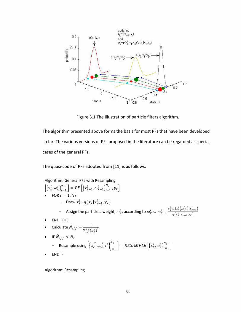
56
Figure 3.1 The illustration of particle filters algorithm.
The algorithm presented above forms the basis for most PFs that have been developed
so far. The various versions of PFs proposed in the literature can be regarded as special
cases of the general PFs.
The quasi-code of PFs adopted from [11] is as follows.
Algorithm: General PFs with Resampling
𝑥𝑘𝑖 , 𝜔𝑘
𝑖 𝑖=1
𝑁𝑠 = 𝑃𝐹 𝑥𝑘−1
𝑖 , 𝜔𝑘−1𝑖
𝑖=1
𝑁𝑠 , 𝑦𝑘
FOR 𝑖 = 1: 𝑁𝑠
- Draw 𝑥𝑘𝑖 ~𝑞 𝑥𝑘 |𝑥𝑘−1
𝑖 , 𝑦𝑘
- Assign the particle a weight, 𝜔𝑘𝑖 , according to 𝜔𝑘
𝑖 ∝ 𝜔𝑘−1𝑖
𝑝 𝑦𝑘 |𝑥𝑘𝑖 𝑝 𝑥𝑘
𝑖 |𝑥𝑘−1𝑖
𝑞 𝑥𝑘𝑖 |𝑥𝑘−1
𝑖 ,𝑦𝑘
END FOR
Calculate 𝑁 𝑒𝑓𝑓 =1
𝜔𝑘𝑖
2𝑁𝑠𝑖=1
IF 𝑁 𝑒𝑓𝑓 < 𝑁𝑇
- Resample using 𝑥𝑘𝑗 ∗
, 𝜔𝑘𝑗, 𝑖𝑗
𝑗=1
𝑁𝑠 = 𝑅𝐸𝑆𝐴𝑀𝑃𝐿𝐸 𝑥𝑘
𝑖 , 𝜔𝑘𝑖
𝑖=1
𝑁𝑠
END IF
Algorithm: Resampling
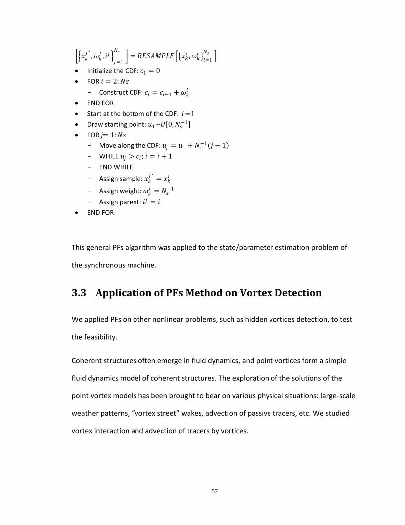
57
𝑥𝑘𝑗 ∗
, 𝜔𝑘𝑗, 𝑖𝑗
𝑗=1
𝑁𝑠 = 𝑅𝐸𝑆𝐴𝑀𝑃𝐿𝐸 𝑥𝑘
𝑖 , 𝜔𝑘𝑖
𝑖=1
𝑁𝑠
Initialize the CDF: 𝑐1 = 0
FOR 𝑖 = 2: 𝑁𝑠
- Construct CDF: 𝑐𝑖 = 𝑐𝑖−1 + 𝜔𝑘𝑖
END FOR
Start at the bottom of the CDF: 1i
Draw starting point: 𝑢1~𝑈 0, 𝑁𝑠−1
FOR j= 1: 𝑁𝑠
- Move along the CDF: 𝑢𝑗 = 𝑢1 + 𝑁𝑠−1 𝑗 − 1
- WHILE 𝑢𝑗 > 𝑐𝑖 ; 𝑖 = 𝑖 + 1
- END WHILE
- Assign sample: 𝑥𝑘𝑗 ∗
= 𝑥𝑘𝑖
- Assign weight: 𝜔𝑘𝑗
= 𝑁𝑠−1
- Assign parent: 𝑖𝑗 = 𝑖
END FOR
This general PFs algorithm was applied to the state/parameter estimation problem of
the synchronous machine.
3.3 Application of PFs Method on Vortex Detection
We applied PFs on other nonlinear problems, such as hidden vortices detection, to test
the feasibility.
Coherent structures often emerge in fluid dynamics, and point vortices form a simple
fluid dynamics model of coherent structures. The exploration of the solutions of the
point vortex models has been brought to bear on various physical situations: large-scale
weather patterns, “vortex street” wakes, advection of passive tracers, etc. We studied
vortex interaction and advection of tracers by vortices.

58
3.3.1 Point vortex model
Point vortices for two-dimensional potential flow are singular solutions to two-
dimensional Euler equations [12], [13], [14].
If the viscous forces are neglected, and the vorticity vector 𝜔 ≡ ∇ × 𝑢, the vorticity-
transport equation corresponding to the Euler equations simplified to two-dimensional
vortex dynamics in (𝑥1, 𝑥2) plane can be written as
𝜕𝜔
𝜕𝑡+ 𝑢 ∙ ∇ 𝜔 = 0 with ∇2𝜓 = 𝜔 (3.7)
where 𝜔 = 𝜔𝑥3 is the vorticity component normal to the (𝑥1, 𝑥2) plane and 𝜓 is the
stream function defined by
𝑢𝑥1= −
𝜕𝜓
𝜕𝑥2𝑢𝑥2
= −𝜕𝜓
𝜕𝑥1 (3.8)
If ω consists of isolated, well-separated vortices, then a reasonable approximation is to
consider the vortices as singularities or “point” vortices. In this case we express the
vorticity field as
ω x, t = Γi(xti − x)
n
i=1
with x0i = xi (3.9)
where Γ𝑖 ≠ 0 is the circulation of vortex 𝑖. By inserting (3.9) in the Euler Equations (3.8)
and using the divergence-free constraint along with the Biot-Savart law, we can bring
PDEs to ODEs, and by including the influence of viscosity and unresolved degrees of
freedom on the vortices, one obtains

59
𝑥 𝑡𝑖 =
Γ𝑗 𝑥𝑡𝑗− 𝑥𝑡
𝑖 ⊥
2𝜋 𝑥𝑡𝑗− 𝑥𝑡
𝑖 2
𝑛
𝑗 ,𝑗≠𝑖
+ 2𝜐𝜉𝑡𝑖 and 𝑥0
𝑖 = 𝑥𝑖 ∈ ℝ2 (3.10)
where 𝜉𝑡𝑖 are zero mean white noise processes and 𝑖 = 1,2, … , 𝑛.
Equation (3.10) shows that the velocity of each vortex is the sum of two terms, namely,
the fluid velocity at the vortex position and a diffusive (stochastic) perturbation
proportional to the fluid viscosity.
3.3.2 Vortex-driven tracer dynamics
Lagrangian meters [12], [13], [14], such as ocean drifters and floats, provide a
substantial part of ocean data which are used to reconstruct mean large-scale currents,
estimate the rate of relative dispersion and give insight into the formation, movement
and interactions of coherent structures such as point vortices and eddies. Based on the
near-continuous data available from these instrumentation networks and to lower
computational costs, we would like to develop more practical techniques required to
analyze and interpret the data for dispersion modeling.
Trajectories of a Lagrangian tracer contain quantitative information about the dynamics
of the underlying flow, and a tracer is advected according to
𝑦 𝑡𝑗
= Γ𝑗 𝑦𝑡
𝑗− 𝑥𝑡
𝑖
2𝜋 𝑦𝑡𝑗− 𝑥𝑡
𝑖 2
𝑛
𝑖
+ 2𝜐𝜂𝑡𝑖 and 𝑦0
𝑗= 𝑦𝑗 ∈ ℝ2, 𝑗 = 1,2, … , m (3.11)
In the context of hidden vortices, the coupling between the dynamical model of the
vortices and the tracers allows us to extract maximal information about the vortices by
tracking the tracers.
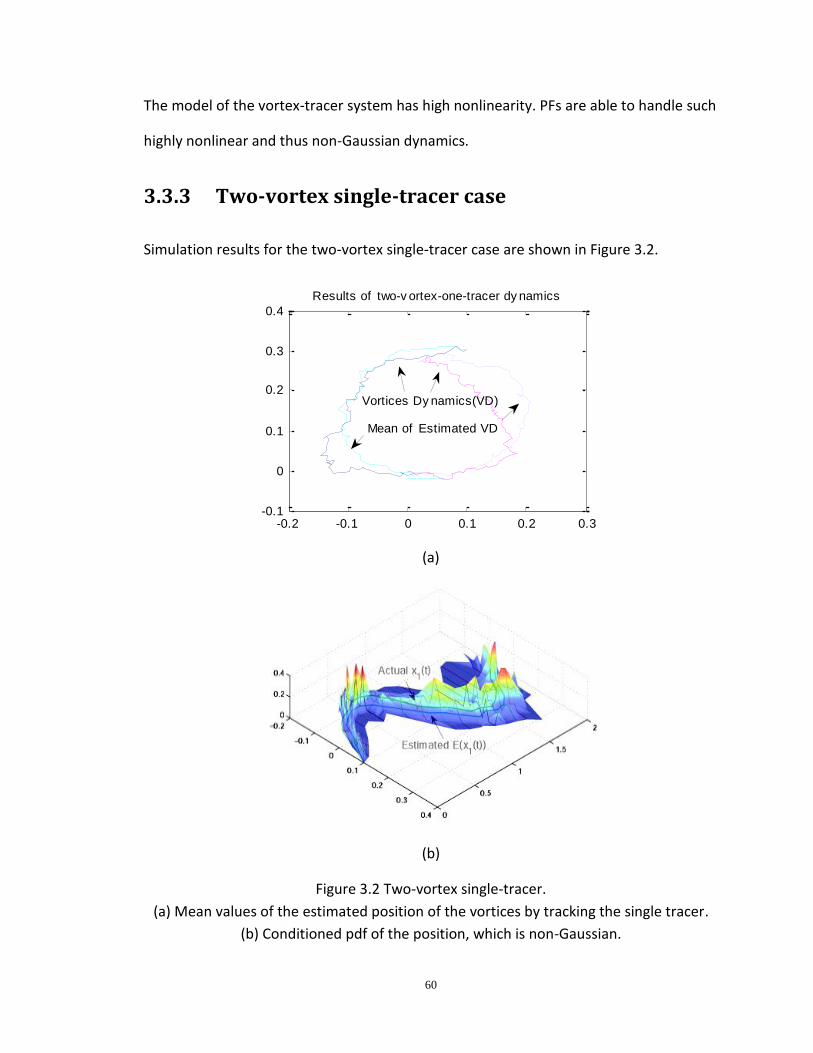
60
The model of the vortex-tracer system has high nonlinearity. PFs are able to handle such
highly nonlinear and thus non-Gaussian dynamics.
3.3.3 Two-vortex single-tracer case
Simulation results for the two-vortex single-tracer case are shown in Figure 3.2.
(a)
(b)
Figure 3.2 Two-vortex single-tracer.
(a) Mean values of the estimated position of the vortices by tracking the single tracer.
(b) Conditioned pdf of the position, which is non-Gaussian.
-0.2 -0.1 0 0.1 0.2 0.3-0.1
0
0.1
0.2
0.3
0.4
Results of two-v ortex-one-tracer dy namics
Vortices Dy namics(VD)
Mean of Estimated VD
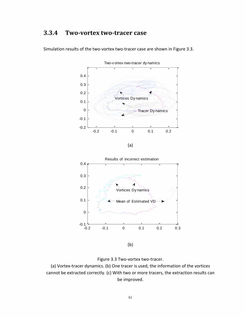
61
3.3.4 Two-vortex two-tracer case
Simulation results of the two-vortex two-tracer case are shown in Figure 3.3.
(a)
(b)
Figure 3.3 Two-vortex two-tracer.
(a) Vortex-tracer dynamics. (b) One tracer is used, the information of the vortices
cannot be extracted correctly. (c) With two or more tracers, the extraction results can
be improved.
-0.2 -0.1 0 0.1 0.2-0.2
-0.1
0
0.1
0.2
0.3
0.4
Two-v ortex-two-tracer dy namics
Vortices Dy namics
Tracer Dy namics
-0.2 -0.1 0 0.1 0.2 0.3-0.1
0
0.1
0.2
0.3
0.4
Results of incorrect estimation
Vortices Dy namics
Mean of Estimated VD

62
(c)
Figure 3.3 Continued.
3.4 Nonlinear Filtering for Electric Machine
State/Parameter Estimation
3.4.1 Machine models
The system considered is a synchronous machine in a power system. We use the
conventions and notations of [15], which are consistent with standard industry
modeling and simulation software. The nonlinear model can be a machine model with
IEEE-Type I exciter/AVR and turbine/governor.
The detailed n-bus, m-machine system model is in the following general form:
-0.1 0 0.1 0.2 0.3-0.1
0
0.1
0.2
0.3
0.4
Results of two-v ortex-two-tracer dy namics
Vortices Dy namics
Mean of Estimated VD
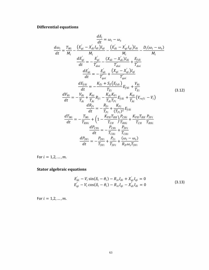
63
Differential equations
𝑑𝛿𝑖
𝑑𝑡= 𝜔𝑖 − 𝜔𝑠
𝑑𝜔𝑖
𝑑𝑡=
𝑇𝑀𝑖
𝑀𝑖−
𝐸𝑞𝑖′ − 𝑋𝑑𝑖
′ 𝐼𝑑𝑖 𝐼𝑞𝑖
𝑀𝑖−
𝐸𝑑𝑖′ − 𝑋𝑞𝑖
′ 𝐼𝑞𝑖 𝐼𝑑𝑖
𝑀𝑖−
𝐷𝑖 𝜔𝑖 − 𝜔𝑠
𝑀𝑖
𝑑𝐸𝑞𝑖′
𝑑𝑡= −
𝐸𝑞𝑖′
𝑇𝑑𝑜𝑖′ −
𝑋𝑑𝑖 − 𝑋𝑑𝑖′ 𝐼𝑑𝑖
𝑇𝑑𝑜𝑖′ +
𝐸𝑓𝑑𝑖
𝑇𝑑𝑜𝑖′
𝑑𝐸𝑑𝑖′
𝑑𝑡= −
𝐸𝑑𝑖′
𝑇𝑞𝑜𝑖′ +
𝑋𝑞𝑖 − 𝑋𝑞𝑖′ 𝐼𝑞𝑖
𝑇𝑞𝑜𝑖′
𝑑𝐸𝑓𝑑𝑖
𝑑𝑡= −
𝐾𝐸𝑖 + 𝑆𝐸 𝐸𝑓𝑑𝑖
𝑇𝐸𝑖𝐸𝑓𝑑𝑖 +
𝑉𝑅𝑖
𝑇𝐸𝑖
𝑑𝑉𝑅𝑖
𝑑𝑡= −
𝑉𝑅𝑖
𝑇𝐴𝑖+
𝐾𝐴𝑖
𝑇𝐴𝑖𝑅𝑓𝑖 −
𝐾𝐴𝑖𝐾𝐹𝑖
𝑇𝐴𝑖𝑇𝐹𝑖𝐸𝑓𝑑𝑖 +
𝐾𝐴𝑖
𝑇𝐴𝑖 𝑉𝑟𝑒𝑓𝑖 − 𝑉𝑖
𝑑𝑅𝑓𝑖
𝑑𝑡= −
𝑅𝑓𝑖
𝑇𝐹𝑖+
𝐾𝐹𝑖
𝑇𝐹𝑖 2𝐸𝑓𝑑𝑖
𝑑𝑇𝑀𝑖
𝑑𝑡= −
𝑇𝑀𝑖
𝑇𝑅𝐻𝑖 + 1 −
𝐾𝑃𝐻𝑇𝑅𝐻
𝑇𝐶𝐻 𝑃𝐶𝐻𝑖
𝑇𝑅𝐻𝑖+
𝐾𝑃𝐻𝑇𝑅𝐻
𝑇𝐶𝐻
𝑃𝑆𝑉𝑖
𝑇𝑅𝐻𝑖
𝑑𝑃𝐶𝐻𝑖
𝑑𝑡= −
𝑃𝐶𝐻i
𝑇𝐶𝐻𝑖 +
𝑃𝑆𝑉𝑖
𝑇𝐶𝐻𝑖
𝑑𝑃𝑆𝑉𝑖
𝑑𝑡= −
𝑃𝑆𝑉𝑖
𝑇𝑆𝑉𝑖+
𝑃𝐶𝑖
𝑇𝑆𝑉𝑖+
𝜔𝑖 − 𝜔𝑠
𝑅𝐷𝜔𝑠𝑇𝑆𝑉𝑖
(3.12)
For 𝑖 = 1,2, … , 𝑚.
Stator algebraic equations
𝐸𝑑𝑖
′ − 𝑉𝑖 sin 𝛿𝑖 − 𝜃𝑖 − 𝑅𝑠𝑖𝐼𝑑𝑖 + 𝑋𝑞𝑖′ 𝐼𝑞𝑖 = 0
𝐸𝑞𝑖′ − 𝑉𝑖 cos 𝛿𝑖 − 𝜃𝑖 − 𝑅𝑠𝑖𝐼𝑞𝑖 − 𝑋𝑑𝑖
′ 𝐼𝑑𝑖 = 0 (3.13)
For 𝑖 = 1,2, … , 𝑚.

64
Network algebraic equations
𝐼𝑑𝑖𝑉𝑖 sin 𝛿𝑖 − 𝜃𝑖 + 𝐼𝑞𝑖𝑉𝑖 cos 𝛿𝑖 − 𝜃𝑖 + 𝑃𝐿𝑖 𝑉𝑖 − 𝑉𝑖𝑉𝑘𝑌𝑖𝑘 cos 𝜃𝑖 − 𝜃𝑘 − 𝛼𝑖𝑘
𝑛
𝑘=1
= 0
𝐼𝑑𝑖𝑉𝑖 cos 𝛿𝑖 − 𝜃𝑖 − 𝐼𝑞𝑖𝑉𝑖 sin 𝛿𝑖 − 𝜃𝑖 + 𝑄𝐿𝑖 𝑉𝑖 − 𝑉𝑖𝑉𝑘𝑌𝑖𝑘 sin 𝜃𝑖 − 𝜃𝑘 − 𝛼𝑖𝑘
𝑛
𝑘=1
= 0
(3.14)
For 𝑖 = 1,2, … , 𝑚.
𝑃𝐿𝑖 𝑉𝑖 − 𝑉𝑖𝑉𝑘𝑌𝑖𝑘 cos 𝜃𝑖 − 𝜃𝑘 − 𝛼𝑖𝑘
𝑛
𝑘=1
= 0
𝑄𝐿𝑖 𝑉𝑖 − 𝑉𝑖𝑉𝑘𝑌𝑖𝑘 sin 𝜃𝑖 − 𝜃𝑘 − 𝛼𝑖𝑘
𝑛
𝑘=1
= 0
(3.15)
For 𝑖 = 𝑚 + 1, 𝑚 + 2, … , 𝑛.
This model has
𝑥𝑖 = 𝛿𝑖 , 𝜔𝑖 , 𝐸𝑞𝑖′ , 𝐸𝑑𝑖
′ , 𝐸𝑓𝑑𝑖 , 𝑉𝑅𝑖 , 𝑅𝐹𝑖 , 𝑇𝑀𝑖 , 𝑃𝑆𝑉𝑖 𝑡
𝑦𝑚𝑖 = 𝐼𝑑𝑖 , 𝐼𝑞𝑖 𝑡
𝑢𝑖 = 𝑉𝑟𝑒𝑓𝑖 , 𝑃𝐶𝑖 𝑡
𝑖 = 1,2, … , 𝑚
𝑦𝑛𝑗 = 𝑉𝑗 , 𝜃𝑗 𝑡
𝑗 = 1,2, … , 𝑛
and 𝑦 = 𝑦𝑚𝑡 , 𝑦𝑛
𝑡 𝑡
(3.16)
The differential-algebraic equations can be summarized as
𝑥 = 𝑓 𝑥, 𝑦, 𝑢
0 = 𝑔 𝑥, 𝑦 or
𝑥𝑘+1 = 𝑓𝑘 𝑥𝑘 , 𝑦𝑘 , 𝑢𝑘
0 = 𝑔𝑘 𝑥𝑘 , 𝑦𝑘 (3.17)
where 𝑥 is the system state, 𝑦 is the output, and 𝑢 is the control vector.
65
Now, considering the system and measurement noises, and modeling uncertainties of
the system, the dynamic model is rewritten as
𝑥 = 𝑓 𝑥, 𝑦, 𝑢 + 𝑣
0 = 𝑔 𝑥, 𝑦 + 𝜆 or
𝑥𝑘+1 = 𝑓𝑘 𝑥𝑘 , 𝑦𝑘 , 𝑢𝑘 + 𝑣𝑘
0 = 𝑔𝑘 𝑥𝑘 , 𝑦𝑘 + 𝜆𝑘 (3.18)
where 𝑣 and 𝜆 are noise or model uncertainties. Equation (3.18) is a more realistic
description of the real system, because of the included noise and uncertainties.
3.4.2 Simulation results
In this section, state estimation results of PFs and EKF are given. Furthermore, we will
also obtain parameter estimation using PFs.
3.4.2.1 State estimation with PST data
Power Systems Toolbox (PST) [16] is used to simulate the WSCC 3-machine, 9-bus
system. A fault is applied at 0.1 s and cleared at 0.2 s. We apply nonlinear filtering on
machine 1. The measurements are current and voltage with added noise 𝜆~𝑁(0, 1%).
For the PFs method, the number of particles used is 𝑁 = 1000. We also suggest that the
initial guess is off the actual value.
Simulation results compared with PST results are shown in Figure 3.4.
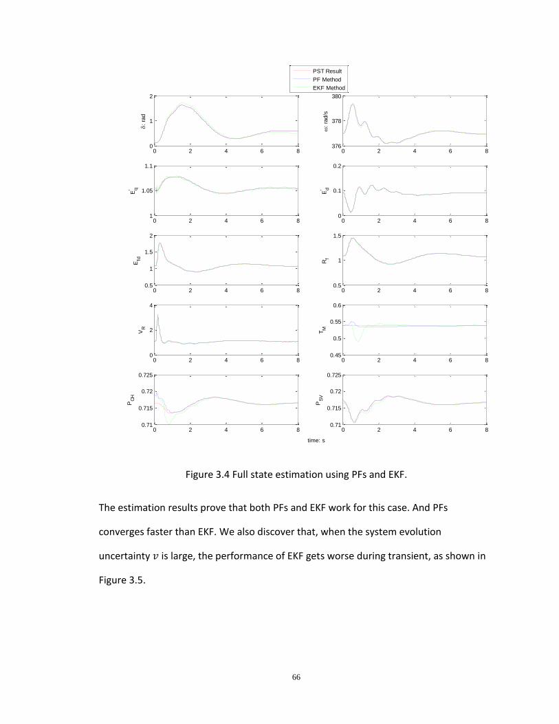
66
Figure 3.4 Full state estimation using PFs and EKF.
The estimation results prove that both PFs and EKF work for this case. And PFs
converges faster than EKF. We also discover that, when the system evolution
uncertainty 𝑣 is large, the performance of EKF gets worse during transient, as shown in
Figure 3.5.
0 2 4 6 80
1
2
:
rad
0 2 4 6 8376
378
380
:
rad/s
0 2 4 6 81
1.05
1.1
Eq
0 2 4 6 80
0.1
0.2
Ed
0 2 4 6 80.5
1
1.5
2
Efd
0 2 4 6 80.5
1
1.5
Rf
0 2 4 6 80
2
4
VR
0 2 4 6 80.45
0.5
0.55
0.6
TM
0 2 4 6 80.71
0.715
0.72
0.725
PC
H
0 2 4 6 80.71
0.715
0.72
0.725
time: s
PS
V
PST Result
PF Method
EKF Method
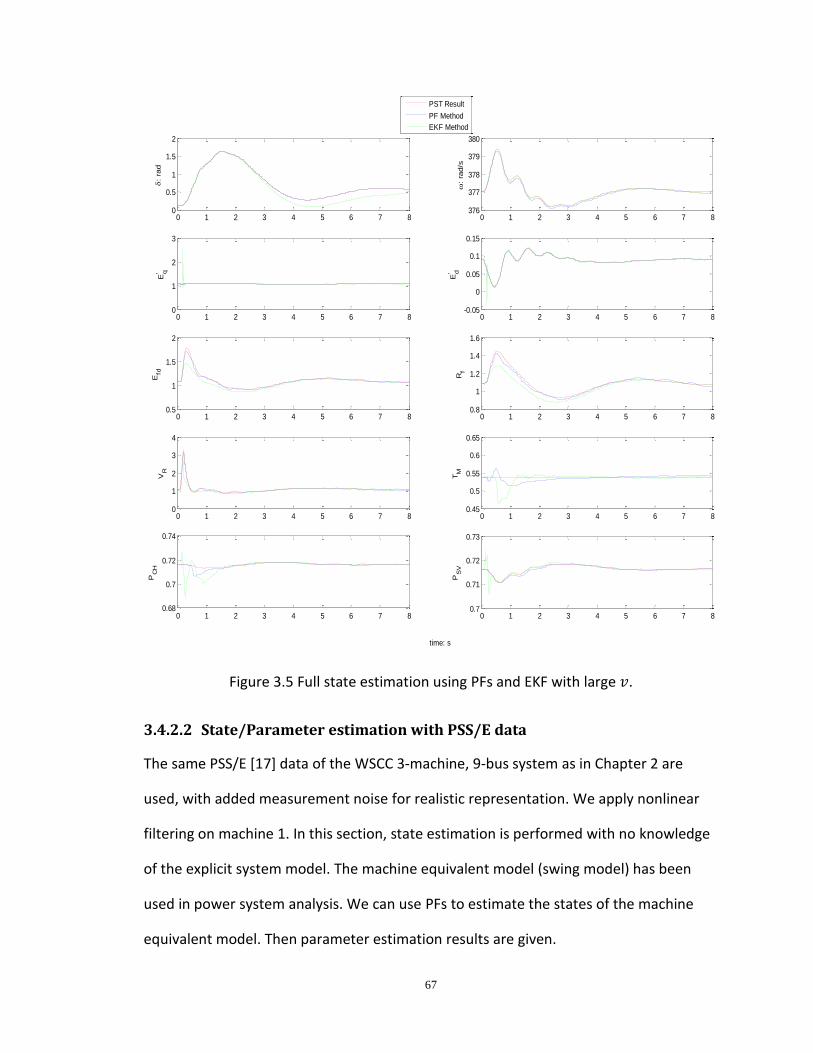
67
Figure 3.5 Full state estimation using PFs and EKF with large 𝑣.
3.4.2.2 State/Parameter estimation with PSS/E data
The same PSS/E [17] data of the WSCC 3-machine, 9-bus system as in Chapter 2 are
used, with added measurement noise for realistic representation. We apply nonlinear
filtering on machine 1. In this section, state estimation is performed with no knowledge
of the explicit system model. The machine equivalent model (swing model) has been
used in power system analysis. We can use PFs to estimate the states of the machine
equivalent model. Then parameter estimation results are given.
0 1 2 3 4 5 6 7 80
0.5
1
1.5
2
:
rad
0 1 2 3 4 5 6 7 8376
377
378
379
380
:
rad/s
0 1 2 3 4 5 6 7 80
1
2
3
Eq
0 1 2 3 4 5 6 7 8-0.05
0
0.05
0.1
0.15
Ed
0 1 2 3 4 5 6 7 80.5
1
1.5
2
Efd
0 1 2 3 4 5 6 7 80.8
1
1.2
1.4
1.6
Rf
0 1 2 3 4 5 6 7 80
1
2
3
4
VR
0 1 2 3 4 5 6 7 80.45
0.5
0.55
0.6
0.65
TM
0 1 2 3 4 5 6 7 80.68
0.7
0.72
0.74
PC
H
0 1 2 3 4 5 6 7 80.7
0.71
0.72
0.73
PS
V
time: s
PST Result
PF Method
EKF Method

68
State estimation
The system evolution equation used in estimation is
𝑑𝛿
𝑑𝑡= 𝜔 − 𝜔𝑠
𝑑𝜔
𝑑𝑡=
𝑃𝑀
𝑀−
𝐷(𝜔 − 𝜔𝑠)
𝑀−
𝑃𝑒
𝑀+ 𝑣1
𝑑𝑃𝑒
𝑑𝑡= 𝑣2
(3.19)
And the measurement is calculated as
𝑃 =𝐸𝑞
′ 𝑉1
𝑋𝑞sin(𝛿 − 𝜃) (3.20)
where
𝐸𝑞
′ =𝑃𝑒 − 𝑋𝑞 − 𝑋𝑑
′ ∙ 𝐼𝑑𝐼𝑞
𝐼𝑞
𝐼𝑑𝑞 = 𝐼 ∙ exp −𝑗(𝛿 −𝜋
2)
(3.21)
This is not exactly the same GENTRA model used in PSS/E. The difference will be
accounted for as the unknown system uncertainties in the algorithm. The particle
number is 𝑁 = 1000. The signal-noise-ratio of measurement is 0.5%. And we assume
the system uncertainty is 𝑣~𝑁 0,0.0012 .
Figure 3.6 gives the estimation results of the PFs method. The estimation results from
EKF are shown in Figure 3.7.

69
Figure 3.6 The PSS/E results and PFs estimation results of machine angle and speed of
machine 1.
0 2 4 6 8 10 12 14 16 18 20-0.12
-0.1
-0.08
-0.06
-0.04
-0.02
0
0.02
0.04
0.06
0.08Machine angle
time: s
rad
PSS/E Result
PF Estimation
0 2 4 6 8 10 12 14 16 18 20-1
-0.8
-0.6
-0.4
-0.2
0
0.2
0.4
0.6
0.8
1x 10
-3 Relative Speed
time: s
rad/s
PSS/E Result
PF Estimation
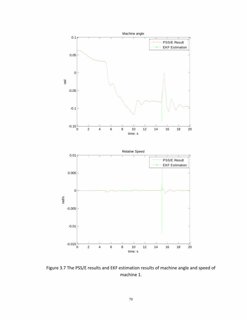
70
Figure 3.7 The PSS/E results and EKF estimation results of machine angle and speed of
machine 1.
0 2 4 6 8 10 12 14 16 18 20-0.15
-0.1
-0.05
0
0.05
0.1Machine angle
time: s
rad
PSS/E Result
EKF Estimation
0 2 4 6 8 10 12 14 16 18 20-0.015
-0.01
-0.005
0
0.005
0.01Relative Speed
time: s
rad/s
PSS/E Result
EKF Estimation
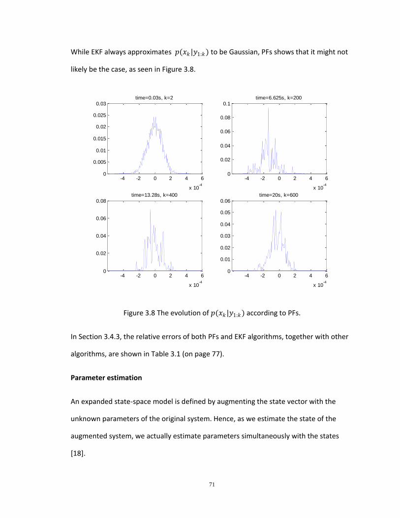
71
While EKF always approximates 𝑝(𝑥𝑘 |𝑦1:𝑘) to be Gaussian, PFs shows that it might not
likely be the case, as seen in Figure 3.8.
Figure 3.8 The evolution of 𝑝(𝑥𝑘 |𝑦1:𝑘) according to PFs.
In Section 3.4.3, the relative errors of both PFs and EKF algorithms, together with other
algorithms, are shown in Table 3.1 (on page 77).
Parameter estimation
An expanded state-space model is defined by augmenting the state vector with the
unknown parameters of the original system. Hence, as we estimate the state of the
augmented system, we actually estimate parameters simultaneously with the states
[18].
-4 -2 0 2 4 6
x 10-4
0
0.005
0.01
0.015
0.02
0.025
0.03time=0.03s, k=2
-4 -2 0 2 4 6
x 10-4
0
0.02
0.04
0.06
0.08
0.1time=6.625s, k=200
-4 -2 0 2 4 6
x 10-4
0
0.02
0.04
0.06
0.08time=13.28s, k=400
-4 -2 0 2 4 6
x 10-4
0
0.01
0.02
0.03
0.04
0.05
0.06time=20s, k=600

72
Here we try to estimate the inertia 𝐻 = 23.64, with initial guess 𝐻𝑖𝑛𝑖𝑡𝑖𝑎𝑙 = 15. We can
see from Figure 3.9 that even though the initial guess is off the true value, PFs can get it
corrected during the evolving process.
𝑚𝑒𝑎𝑛 𝐻𝑒𝑠𝑡𝑖𝑚𝑎𝑡𝑖𝑜𝑛 ,16:20 = 22.84
Figure 3.9 Estimated inertia H.
Figure 3.9 also shows that augmented EKF cannot properly estimate such a parameter.
Stochastic estimation
Stochastic parameters can also be obtained using augmented PFs.
As we know, the swing model used in PFs estimation is not the same as the GANTRA
model in PSS/E; the standard deviation of the difference between speed derived from
the swing model with no uncertainties and the PSS/E result is 𝜍𝜔 = 3.3296𝑒 − 5. The
0 2 4 6 8 10 12 14 16 18 2010
12
14
16
18
20
22
24
26
time: s
Inert
ia
Inertia Value
PF Estimation
EKF Estimation
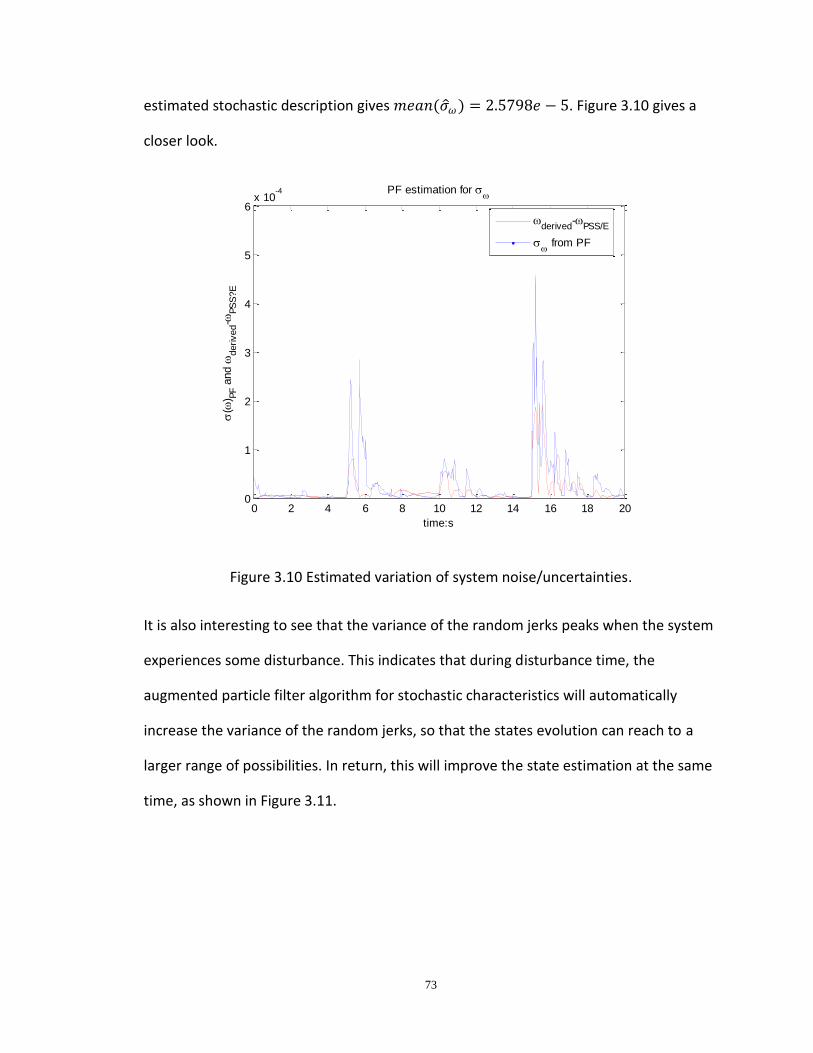
73
estimated stochastic description gives 𝑚𝑒𝑎𝑛(𝜍 𝜔) = 2.5798𝑒 − 5. Figure 3.10 gives a
closer look.
Figure 3.10 Estimated variation of system noise/uncertainties.
It is also interesting to see that the variance of the random jerks peaks when the system
experiences some disturbance. This indicates that during disturbance time, the
augmented particle filter algorithm for stochastic characteristics will automatically
increase the variance of the random jerks, so that the states evolution can reach to a
larger range of possibilities. In return, this will improve the state estimation at the same
time, as shown in Figure 3.11.
0 2 4 6 8 10 12 14 16 18 200
1
2
3
4
5
6x 10
-4
time:s
(
) PF a
nd
derived-
PS
S?E
PF estimation for
derived
-PSS/E
from PF

74
Figure 3.11 Estimated relative speed with unknown system variation.
We also tried to use augmented EKF to estimate this stochastic characteristic; as in the
previous section, it fails to get the correct estimation.
3.4.3 Particle filters with smoother
Particle filters with smoother can help yield more accurate state estimation and even
out the wiggles caused by random jerks.
Several smoother approaches have been implemented: We can reach arbitrarily precise
posterior density simply by increasing the number of particles/samples, but this is very
computationally costly and more suitable for lower order systems. We can also increase
the accuracy of approximation by generating 𝑑 different realizations of system noise for
each particle 𝑥𝑘𝑖 . Then we obtain 𝑁 × 𝑑 particles at step 1, and 𝑁 particles at step 3 by
resampling from 𝑁 × 𝑑 particles. The third approach is 𝐿-lag fixed lag smoother [19].
0 2 4 6 8 10 12 14 16 18 20-8
-6
-4
-2
0
2
4
6
8
10
12x 10
-4
time:s
rela
tive s
peed:
rad/s
PSS/E Result
Augmented PF Estimation

75
The 𝐿-lag fixed lag smoother is a modification of the PFs algorithm in Section 3.2.2. Let
𝑠𝑘−𝐿|𝑘−1𝑖 , … , 𝑠𝑘−1|𝑘−1
𝑖 denote the 𝑖𝑡 realization of the conditional joint density
𝑝 𝑥𝑘−𝐿 , … , 𝑥𝑘−1|𝑦𝑘−1 . Then prediction could be
𝑝 𝑗 𝑘−1 𝑖 =
𝑠 𝑗 𝑘−1 𝑖 𝑗 = 𝑘 − 𝐿, … , 𝑘 − 1
𝑓(𝑠 𝑘−1 𝑘−1 𝑖 , 𝑦𝑘 , 𝑢𝑘 , 𝑣𝑘) 𝑗 = 𝑘
(3.22)
The correction step in Section 3.2.2 could be
Step 3s: Generate 𝑠𝑘−𝐿|𝑘𝑖 , … , 𝑠𝑘−1|𝑘
𝑖 , 𝑠𝑘|𝑘𝑖 by resampling 𝑠𝑘−𝐿|𝑘
𝑖 , … , 𝑠𝑘−1|𝑘𝑖 , 𝑝𝑘|𝑘−1
𝑖 with
the weight obtained in step 2. 𝑝 𝑥𝑘−𝐿:𝑘 𝑦1:𝑘 ≈ 𝜔𝑘𝑖 𝛿 𝑥𝑘−𝐿:𝑘 − 𝑠𝑘−𝐿:𝑘
𝑖 𝑁𝑖=1 .
The results are shown in Figure 3.12. Table 3.1 compares the results of different
algorithms. The relative error of 𝑥 is defined as
휀 𝑥 ≜
1𝑛
𝑥 𝑖 − 𝑥𝑖 2𝑛𝑖=1
1𝑛
𝑥𝑖 2𝑛𝑖=1
From Table 3.1 we can see that PFs can achieve better estimation than EKF. Increasing
the particle numbers or by adding smoothers will improve the results of the PFs.

76
(a)
(b)
Figure 3.12 Fixed lag smoother 𝐿 = 10.
0 2 4 6 8 10 12 14 16 18 20-0.12
-0.1
-0.08
-0.06
-0.04
-0.02
0
0.02
0.04
0.06
0.08Machine angle
time: s
rad
PSS/E Result
PF Estimation
PF with L-lag Smoother
0 2 4 6 8 10 12 14 16 18 20-1
-0.8
-0.6
-0.4
-0.2
0
0.2
0.4
0.6
0.8
1x 10
-3 Relative Speed
time: s
rad/s
PSS/E Result
PF Estimation
PF with L-lag Smoother
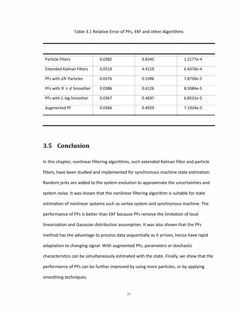
77
Table 3.1 Relative Error of PFs, EKF and other Algorithms
Algorithms 𝜺(𝜹) 𝜺 𝝎 − 𝝎𝒔 𝜺 𝝎
Particle Filters 0.0382 0.8345 1.2177e-4
Extended Kalman Filters 0.0519 4.4119 6.4376e-4
PFs with 𝑑𝑁 Particles 0.0376 0.5396 7.8730e-5
PFs with 𝑁 × 𝑑 Smoother 0.0386 0.6126 8.9384e-5
PFs with 𝐿-lag Smoother 0.0367 0.4697 6.8531e-5
Augmented PF 0.0366 0.4929 7.1924e-5
3.5 Conclusion
In this chapter, nonlinear filtering algorithms, such extended Kalman filter and particle
filters, have been studied and implemented for synchronous machine state estimation.
Random jerks are added to the system evolution to approximate the uncertainties and
system noise. It was shown that the nonlinear filtering algorithm is suitable for state
estimation of nonlinear systems such as vortex system and synchronous machine. The
performance of PFs is better than EKF because PFs remove the limitation of local
linearization and Gaussian distribution assumption. It was also shown that the PFs
method has the advantage to process data sequentially as it arrives, hence have rapid
adaptation to changing signal. With augmented PFs, parameters or stochastic
characteristics can be simultaneously estimated with the state. Finally, we show that the
performance of PFs can be further improved by using more particles, or by applying
smoothing techniques.
78
Other readings can be found in [20]-[27].
3.6 References
[1] V. Miranda and J. P. Saraiva, "Fuzzy modelling of power system optimal load flow,"
IEEE Transactions on Power Systems, vol. 7, no. 2, pp. 843-849, May 1992.
[2] P. Carpentier, G. Cohen, J. C. Culioli, and A. Renaud, "Stochastic optimization of unit
commitment: A new decomposition framework," IEEE Transactions on Power
Systems, vol. 11, no. 2, pp. 1067-1076, May 1996.
[3] S. Takriti, J. R. Birge, and E. Long, "A stochastic model for the unit commitment
problem," IEEE Transactions on Power Systems, vol. 11, no. 2, pp. 1497-1508, Aug.
1996.
[4] J. W. Feltes et al., "Deriving model parameters from field test measurements," IEEE
Computer Applications in Power, vol. 15, no. 4, pp. 30-36, Oct. 2002.
[5] IEEE Task Force on Load Representation for Dynamic Performance, "Load
representation for dynamic performance analysis," IEEE Transactions on Power
Systems, vol. 8, no. 2, pp. 472-482, May 1993.
[6] M. West and J. Harrison, Bayesian Forecasting and Dynamic Models, 2nd ed. New
York, NY: Springer-Verlag, 1997.
[7] R. Dhaouadi, N. Mohan, and L. Norum, "Design and implementation of an extended
Kalman filter for the state estimation of a permanent magnet synchronous motor,"
IEEE Transactions on Power Electronics, vol. 6, pp. 491-497, July 1991.
[8] Y.-R. Kim, S.-K. Sul, and M.-H. Park, "Speed sensorless vector control of induction
motor using extended Kalman filter," IEEE Transactions on Industry Applications,
vol. 30, pp. 1225-1233, Sep. 1994.
[9] B. Terzic and M. Jadric, "Design and implementation of the extended Kalman filter
for the speed and rotor position estimation of brushless DC motor," IEEE
Transactions on Industrial Electronics, vol. 48, no. 6, pp. 1065-1073, Dec. 2001.
[10] A. Qiu, B. Wu, and H. Kojori, "Sensorless control of permanent magnet synchronous
motor using extended Kalman filter," in Canadian Conference on Electrical and
79
Computer Engineering, 2004, vol. 3, 2004, pp. 1557-1562.
[11] M. S. Arulampalam, S. Maskell, N. Gordon, and T. Clapp, "A tutorial on particle
filters for online nonlinear/non-Gaussian Bayesian tracking," IEEE Transactions on
Signal Processing, vol. 50, no. 2, pp. 174-188, Feb. 2002.
[12] O. Agullo and A. D. Verga, "Effect of viscosity in the dynamics of two point vortices:
Exact results," Physical Review E., vol. 63, no. 5, pp. 56304-56317, 2001.
[13] P. G. Saffman, Vortex Dynamics. Cambridge: Cambridge University Press, 1992.
[14] P. K. Newton, The N-Vortex Problem: Analytical Techniques. Berlin, Germany:
Springer-Verlag, 2001.
[15] P. W. Sauer and M. A. Pai, Power System Dynamics and Stability. Upper Saddle
River, NJ: Prentice Hall, 1998.
[16] J. Chow and G. Rogers. "Power Systems Toolbox." [Online]. Available:
http://www.eagle.ca/~cherry/pst.htm.
[17] PSS/E, Power system simulator for engineering. Schenectady, NY: Siemens - Power
Technologies Inc.
[18] G. Kitagawa, "A self-organizing state-space model," Journal of American Statistical
Association, vol. 93, no. 443, pp. 1203-1215, 1998.
[19] G. Kitagawa, "Monte Carlo filter and smoother for non-Gaussian nonlinear state
space models," Journal of Computational and Graphical Statistics, vol. 5, no. 1, pp.
1-25, March 1996.
[20] A. Doucet, N. J. Gordon, and V. Krishnamurthy, "Particle filters for state estimation
of jump Markov linear systems," IEEE Transactions on Signal Processing, vol. 49, no.
3, pp. 613-624, March 2001.
[21] A. Doucet and V. B. Tadid, "Parameter estimation in general state-space models
using particle methods," Annals of the Institute of Statistical Mathematics, vol. 55,
no. 2, pp. 409-422, June 2003.
[22] G. Poyiadjis, A. Doucet, and S. S. Singh, "Maximum likelihood parameter estimation
in general state-space models using particle methods," August 2005. [Online].
Available: http://www.cs.ubs.ca/~arnaud/poyiadjis_doucet_singh_

80
parameterestimationparticlesJM05.pdf.
[23] C. Andrieu, A. Doucet, and V. Tadid, "Online simulation-based methods for
parameter estimation in nonlinear non-Gaussian state-space models," in
Proceedings on IEEE Conference of Decision Control, 2005, pp. VI70-V172.
[24] S. Liu, N. S. Namachchivaya, P. W. Sauer, and J. H. Park, "Detection of hidden
vortices in multi-sensor environments," in 21st Canadian Congress of Applied
Mechanics, Toronto, Canada, 2007.
[25] S. Liu, P. Sauer, and N. S. Namachchivaya, "Techniques for dynamic state estimation
of machines in power system," in World Scientific and Engineering Academy and
Society PE07, Beijing, China, Sep. 2007, pp. 1-6.
[26] A. Barreiro, S. Liu, N. S. Namachchivaya, P. W. Sauer, and R. B. Sowers, "Data
assimilation in the detection of vortices," in Applications of Nonlinear Dynamics
Model and Design of Complex Systems Series: Understanding Complex Systems, V.
In, P. Longhini, and A. Palacios, Eds. New York, NY: Springer, 2009, pp. 47-60.
[27] A. Barreiro, S. Liu, N. S. Namachchivaya, P. W. Sauer, and R. B. Sowers, "Data
assimilation in the detection of vortices," in 6th EUROMECH Nonlinear Dynamics
Conference, 2008, Saint Petersburg, Russia, 2008.
81
CHAPTER 4
MODEL REDUCTION WITH BALANCED
TRUNCATION
4.1 Introduction
Due to their constantly increasing size and complexity, power systems are among the
largest and most intricate engineered systems in operation today. Power system
analysis has to tackle high-order modeling. And even more complicated analysis will be
performed to study the system behaviors with upcoming changes and innovations in the
power industry. The dimension of such mathematical models may easily reach the order
of several thousand for applications like dynamic simulation or trajectory sensitivity
analysis. Therefore, it will become very computationally costly while the final analysis
results may have unnecessary portions, leading to high investments but with no
apparent advantages. Equation Chapter 4 Section 1
In such cases, it is obvious that there is a need for a low-order model to replace the
original system, so that the computational problem can be avoided while the main
characteristics are still preserved [1 – 6]. Then the low-order model can be used to
perform other analyses, such as damping control [3], stability study [4], cascading failure
analysis [5], etc.
We can partition a power system into two areas for system analysis: the study area and
the external area [7]. The study area contains the variables of interest, and therefore it
is modeled in detail. The external area is important only insofar as it influences the

82
analysis in the study area and therefore is represented by a linear model which can be
further replaced by a reduced-order system. Then we focus on the model reduction for
the external area.
The model reduction methods for power system analysis can be roughly classified into
two categories: engineering methods and mathematical methods [8]. Engineering
methods are usually based on physical considerations, such as grouping similarly
behaved generators into one [2] , [9], or ignoring some phenomena which are assumed
to be of minor significance [10]. In mathematical methods, the size of state equations is
reduced while keeping the major oscillation modes. The modes are selected based on
some mathematical criteria to assure an acceptable level of accuracy, such as
modal/eigenvalue analysis [8], Krylov subspaces [11], etc. Engineering methods give a
clear connection between the reduced-order system and the original system; however,
as systems grow larger, such methods generally become more complex and result in a
considerable computational effort. They also typically require either the construction of
new matrices or substantial changes in the system structure, both of which further
complicate the procedure.
The main objective in this chapter is to develop a mathematical method to reduce the
order of large power systems. While most mathematical methods for power system
order reduction are focused on either the Jacobian matrix analysis or input-state
analysis, the approach we propose in this chapter is more interested in input-output
behavior. It directly emphasizes the factors that have the most influence on the analysis
in the study area, and so will result not only in straightforward understanding but also in
simpler representation.
83
Balanced truncation is a known projection model reduction method which delivers high
quality reduced models. It has been applied in spacecraft modeling, control system
design, and other areas of large dimension modeling [12]. In this chapter, the
framework for using the balanced truncation method in power systems is provided.
Additionally, the sensitivity analysis is performed to further include consideration of the
nonlinear nature of power systems.
The rest of the chapter is organized as follows. An overview of other model reduction
methods in power systems is introduced. The balanced truncation algorithm is then
presented. Simulation results are then given to illustrate the application of the balanced
truncation algorithm and sensitivity analysis for power systems.
4.2 Related Work
The dynamic behavior of a large electric power system can be described by a set of
differential-algebraic equations (DAE):
𝑥 = 𝑓 𝑥, 𝑦
0 = 𝑔 𝑥, 𝑦 (4.1)
where 𝑥 is the set of state variables of all the dynamic devices, such as generators,
exciters and governors, and 𝑦 represents voltage magnitudes and angles at the buses.
In an interconnected power system pool it is essential that a large data set be reduced
to a size suitable for the various tasks in dynamic security assessment and analysis. We
are going to discuss several model reduction methodologies briefly in this section.

84
Impact ignorance
These methods identify the components or dynamics which have limited impact on the
system dynamics, and hence can be neglected during modeling. Time-scale
decomposition is one such method which separates the fast network system and slow
machine mechanical system [10]. Using a two-dimensional classical generator model to
replace the detailed generator model, while neglecting other control system
phenomena, falls into this category. While such methods might not be sufficient for
model reduction of large electric power systems, they do form a base for other methods
to build upon. Most, if not all, other model reduction methods have included
phenomena ignorance reduction.
Coherency
Coherency is the most used model reduction in power systems. The basic idea is to
reduce groups of generators in the system, which results in an appropriate model with
fewer dynamic variables. The process can be divided into three stages: coherency
identification, generator aggregation and network reduction [13].
To identify coherency, some assumptions are made to greatly simplify the process [13] –
[20].
Nongenerator dynamics can be ignored.
Classical generator model may be used.
The linearized system model preserves the trends of coherency well.
A variety of methods and algorithms have been suggested to identify coherency,
utilizing concepts such as electromechanical distances [14] [15], singular points [16],
85
clustering of swing curves [13], analysis of eigenvectors [17], Liapunov function [18],
energy function [19], artificial neural networks [20], etc.
After a group of coherent generators is identified, we then can aggregate these
generators to one or a few equivalent generators. Generally, generator aggregation can
take one of two forms: classical aggregation and detailed aggregation. Classical
aggregation represents the coherent generator group by a classical generator model,
while detailed aggregation uses a detailed generator model with an equivalent exciter,
governor and stabilizer, if the coherent generators have similar control systems.
Once equivalent generators are determined for the coherent groups, a network
reduction is performed.
The coherency-based approach to forming the dynamic equivalent of a power system
can obtain an accurate and reduced order model, if the coherency behavior of
synchronous generators is obtained accurately. Hence, most methods in this category
suffer from one or more limitations such as high computational expense, local validation,
repeated evaluation, a priori knowledge, etc.
Epsilon decomposition
The idea of epsilon decomposition is that given a matrix 𝐴 = [𝑎𝑖𝑗 ] and a value of
parameter 휀 > 0, all elements satisfying 𝑎𝑖𝑗 < 휀 are set to zero. The resulting
sparsified matrix is then permuted into a block diagonal form, and all variables in the
same block are considered to be strongly coupled.
86
It is obvious that results obtained by applying epsilon decompositions will depend on
the choice of parameter 휀. The resulting equivalent model in [21] is about half the size
of the original system order, which is not substantial or attracting.
Krylov subspaces
In [11], a Krylov subspaces projection based moment matching approach is provided.
Like balanced truncation, this method measures the accuracy of the reduced order
system by using the transfer function. The Krylov subspace projection can be described
as follows.
A 𝑗𝑡 dimensional Krylov subspace corresponding to matrix 𝐴 and vector 𝑏 is denoted
𝒦𝑗 𝐴, 𝑏 and is defined as
𝒦𝑗 𝐴, 𝑏 = 𝑠𝑝𝑎𝑛 𝑏, 𝐴𝑏, 𝐴2𝑏, … , 𝐴𝑗−1𝑏 (4.2)
Projection extracts the approximate solution of dimension 𝑀 from the search space
𝒦𝑗 𝐴, 𝑏 .
The subspace can be represented via rectangular matrix 𝑉, whose column forms the
bases of the respective subspace. Then the transformation and truncation can be
performed using the matrix 𝑉. The Krylov subspace based moment matching technique
approximates the system transfer function around certain interpolation points of
interest by using Krylov subspaces generated by

87
𝒦𝐽𝑏𝑘 𝐴 − 𝜍𝐼 −1, 𝑏
𝐾
𝑘=1
𝒦𝐽𝑐𝑘 𝐴 − 𝜍𝐼 −𝑇 , 𝑐
𝐾
𝑘=1
(4.3)
where 𝜍 is the interpolation point, and 𝐴, 𝑏, 𝑐 are from a linear, single-input, single-
output, time-invariant system:
𝑥 = 𝐴𝑥 + 𝑏𝑢𝑦 = 𝑐𝑇𝑥
(4.4)
If 𝑉 and 𝑍 are chosen to be bases for the union of the Krylov subspaces mentioned
above (4.3), respectively, then the moments of the reduced system match the moments
of the original system up to a number relative to the dimension of the Krylov subspaces.
The reduced system is obtained as follows.
Decompose the right and left nonsingular transformation as
𝑇𝑟𝑖𝑔𝑡 = 𝑉𝑁×𝑛 𝑉+𝑁×(𝑁−𝑛)
𝑇𝑙𝑒𝑓𝑡 = 𝑍𝑁×𝑛 𝑍+𝑁×(𝑁−𝑛) (4.5)
Apply this transformation to (4.4):
𝑍𝑇𝑉 𝑍𝑇𝑉+
𝑍+𝑇𝑉 𝑍+
𝑇𝑉+
𝑥
x + =
𝑍𝑇𝐴𝑉 𝑍𝑇𝐴𝑉+
𝑍+𝑇𝐴𝑉 𝑍+
𝑇𝐴𝑉+
𝑥 𝑥 +
+ 𝑍𝑇𝑏𝑍+
𝑇𝑏 𝑢
𝑦 = 𝑐𝑇𝑉 𝑐𝑇𝑉+ 𝑥 𝑥 +
Then, assuming 𝑍𝑇𝑉 is nonsigular, the leading subsystem is retained to form the
reduced model:

88
𝑥 = 𝑍𝑇𝑉 −1𝑍𝑇𝐴𝑉𝑥 + 𝑍𝑇𝑉 −1𝑍𝑇𝑏𝑢
𝑦 = 𝑐𝑇𝑉𝑥 (4.6)
Various approaches have been developed to construct the bases for a Krylov subspace.
The best known Krylov subspace methods are the Arnoldi, Lanczos, GMRES (generalized
minimum residual) and BiCGSTAB (stabilized biconjugate gradient) methods. Since it is
not our primary interest here, more details can be found in [22].
There are two major drawbacks of the Krylov subspace based moment matching
method. First, the performance is good in a limited range of frequencies. Stability and
passivity are not necessarily preserved in the reduced order system, and there is no
global approximation error bound. Second, it emphasizes the relation between input
and state, or between state and output, instead of directly considering the input-output
connection, which not only brings in redundancy but also risks losing important
connections between input and output.
4.3 BT Algorithm
Balanced truncation is an important projection model reduction method which delivers
high-quality reduced order models by carefully choosing projection subspaces.
Given the system
𝑥 = 𝐴𝑥 + 𝐵𝑢𝑦 = 𝐶𝑇𝑥 + 𝐷𝑢
(4.7)
the transfer function is denoted by
89
𝐺 𝑠 = 𝐶 𝑠𝐼 − 𝐴 −1𝐵 + 𝐷 (4.8)
The balanced truncation makes use of two crucial quantities, called the reachability and
observability Gramians. The reachability Gramian is
𝑊𝑟 0, 𝑡𝑓 ∶= 𝑒𝐴𝜏𝐵𝐵𝑇𝑡𝑓
0
𝑒𝐴𝑇𝜏𝑑𝜏 (4.9)
And the observability Gramian is
𝑊𝑜 0, 𝑡𝑓 ∶= 𝑒𝐴𝑇𝜏𝐶𝑇𝐶𝑡𝑓
0
𝑒𝐴𝜏𝑑𝜏 (4.10)
The balanced truncation method consists in transforming the state space system into a
balanced form, together with a truncation of those states that are both difficult to reach
and difficult to observe.
An important property of this method is that the asymptotic stability is preserved in the
reduced-order system. Moreover, the existence of a priori error bounds [12] allows an
adaptive choice of the state space dimension of the reduced model, depending on how
accurate an approximation is needed.
4.3.1 Gramians and Hankel singular values
Frequently, system 𝐺(𝑠) is assumed asymptotically stable and the controllability and
observability Gramians 𝑊𝑟 and 𝑊𝑜 are then solutions of two Lyapunov equations:
𝐴𝑊𝑟 + 𝑊𝑟𝐴𝑇 = −𝐵𝐵𝑇 , 𝐴𝑇𝑊𝑜 + 𝑊𝑜𝐴 = −𝐶𝑇𝐶 (4.11)

90
The square roots of the eigenvalues of the product 𝑊𝑟𝑊𝑜 are so-called Hankel singular
values 𝜍 of the system 𝐺(𝑠):
𝜍𝑖 = 𝜆𝑖 𝑊𝑟𝑊𝑜 (4.12)
In many cases, the eigenvalues of 𝑊𝑟 , 𝑊𝑜 as well as the Hankel singular values 𝜍 decay
very rapidly.
We now consider transformation of the above system such that 𝑥 = 𝑇𝑥 , 𝑇 ∈ 𝑅𝑛×𝑛 . We
have
𝐴 = 𝑇−1𝐴𝑇𝐵 = 𝑇−1𝐵𝐶 = 𝐶𝑇𝐷 = 𝐷
(4.13)
And
𝑊𝑟 = 𝑇−1𝑊𝑟𝑇
−𝑇
𝑊𝑜 = 𝑇𝑇𝑊𝑜𝑇
(4.14)
The reachable and observable system 𝐺(𝑠) is called Lyapunov balanced if
𝑊𝑟 = 𝑊𝑜
= Σ = 𝑑𝑖𝑎𝑔 Σ1, Σ2 = 𝑑𝑖𝑎𝑔 𝜍1, 𝜍2, … , 𝜍𝑘 , 𝜍𝑘+1, … , 𝜍𝑛 (4.15)
where 𝜍1 > 𝜍2 > ⋯ > 𝜍𝑘 > 𝜍𝑘+1 > ⋯ > 𝜍𝑛 , and Σ1 = 𝑑𝑖𝑎𝑔 𝜍1, 𝜍2, … , 𝜍𝑘 and
Σ2 = 𝑑𝑖𝑎𝑔 𝜍𝑘+1, … , 𝜍𝑛 .
It should be pointed out that, while the eigenvalues (or system modes) are invariant
under similarity 𝑇, the eigenvalues of the Gramians are not. However, the eigenvalues
of the product of the Gramians — that is, the Hankel singular values — are easily seen to
91
be similarity invariant. The transformation 𝑇 to get the balanced 𝑊𝑟 , 𝑊𝑜
is called a
contragradient transformation.
By truncating the states that are simultaneously difficult to reach and difficult to
observe, which correspond to small Hankel singular values 𝜍𝑘+1, … , 𝜍𝑛 , we can get the
reduced order system.
𝐺𝑟 𝑠 = 𝐶𝑟 𝑠𝐼 − 𝐴𝑟 −1𝐵𝑟 + 𝐷𝑟 (4.16)
The reduced order system satisfies
𝐺 𝑠 − 𝐺𝑟 𝑠 ℋ∞≤ 2 𝜍𝑖
𝑛
𝑖=𝑘+1
and 𝐺 𝑠 − 𝐺𝑟 𝑠 ℋ∞≥ 𝜍𝑘 (4.17)
which equally holds if Σ2 = 𝑑𝑖𝑎𝑔 𝜍𝑛 .
A state-space balancing algorithm is described below [23].
Compute Cholesky factors of the Gramians (the Gramians themselves are not
actually formed). Let 𝐿𝑟 and 𝐿𝑜 denote the lower triangular Cholesky factors of
the Gramians 𝑊𝑟 and 𝑊𝑜 , i.e.,
𝑊𝑟 = 𝐿𝑟𝐿𝑟 𝑇 𝑊𝑜 = 𝐿𝑜𝐿𝑜𝑇 (4.18)
Compute singular value decomposition
𝐿𝑜𝑇𝐿𝑟 = 𝑈ΛV 𝑇 (4.19)
Form the balancing transformation
92
𝑇 = 𝐿𝑟V Λ−1/2 (4.20)
Form the balanced state-space matrices 𝐴 , 𝐵 , 𝐶 and 𝐷 .
Several other approaches exist for balancing the system, such as Schur method, square
root method, etc. Further details and references can be found in [12], [23 - 25]. Other
topics including balanced truncation for model reduction of nonlinear systems, time-
varying systems are discussed in [26 - 28].
4.4 Simulation in Power System
Following the notation in [11], we have an external system connected with study area
with 𝑝 tie-lines. And we apply model reduction for the external system.
The two-dimensional classic model is used for the study of model reduction of the
external area.
𝛿 𝑖 = 𝜔𝑖 − 𝜔𝑠
2𝐻𝑖
𝜔𝑠𝜔𝑖 = 𝑇𝑀𝑖
− 𝐷𝑖 𝜔𝑖 − 𝜔𝑠 − 𝐸𝑖2𝐺𝑖𝑖 − 𝐸𝑖 𝐸𝑗 𝐺𝑖𝑗 𝑐𝑜𝑠 𝛿𝑖 − 𝛿𝑗 + 𝐸𝑗 𝐵𝑖𝑗 𝑠𝑖𝑛 𝛿𝑖 − 𝛿𝑗
𝑚
𝑗 =1𝑗≠𝑖
−𝐸𝑖 𝐸𝑗𝐺𝑖𝑗 𝑐𝑜𝑠 𝛿𝑖 − 𝜃𝑗 + 𝐸𝑗𝐵𝑖𝑗 𝑠𝑖𝑛 𝛿𝑖 − 𝜃𝑗
𝑝
𝑗 =1
(4.21)
where 𝑚 is the number of generators, and 𝑝 is the number of tie-lines. 𝐻𝑖 and 𝐷𝑖
represent the inertia and damping coefficients, respectively, of machine 𝑖. The detailed
description of how to deduct the (4.21) from the detailed model of the system can be
found in [29].

93
We now assume the “internal” nodes of the external system are connected to the study
area via 𝑝 tie-lines. (This assumption can be easily removed by a little extra calculation
using the admittance matrix. To be comparable with the work in [30], we will follow this
assumption for now.)
The 16-machine, 68-bus system is assumed to be the study area, and the 50-machine,
145-bus system is taken as the external area, the configuration of the study and external
areas is shown in Figure 4.1.
Figure 4.1 The topology of study and external areas.
The inputs of the external system, denoted as 𝑢, are considered to be the angles and
voltage amplitudes of the 𝑝 connected buses belonging to the study area. The outputs
of the system, denoted as 𝑦, are considered to be the angles and voltages of the 𝑝
corresponding buses from the external system.
Linearizing system (4.21) around an equilibrium point, we can get
∆𝛿
∆𝜔 =
0 𝐼𝐴 −𝑀
∆𝛿∆𝜔
+ 0𝐵 ∆𝑢
𝑦 = 𝐶 𝑇 0 ∆𝛿∆𝜔
(4.22)
where
Study Area
𝑉1, 𝜃1
16-machine
𝑉2 , 𝜃2
68-bus ⋮
system
𝑉𝑝 , 𝜃𝑝
𝛿𝑙1 External
Area
𝛿𝑙2 50-machine
⋮ 145-bus
𝛿𝑙𝑝 system

94
𝐴 𝑖, 𝑗 =𝜔𝑠
2𝐻𝑖𝐸𝑖𝐸𝑗 −𝐺𝑖𝑗 sin 𝛿𝑖𝑗
𝑜 + 𝐵𝑖𝑗 cos 𝛿𝑖𝑗𝑜 𝑖, 𝑗 = 1, … , 𝑚
𝐴 𝑖, 𝑖 =𝜔𝑠
2𝐻𝑖 𝐸𝑗 𝐺𝑖𝑗 sin 𝛿𝑖𝑗
𝑜 − 𝐵𝑖𝑗 cos 𝛿𝑖𝑗𝑜
𝑚
𝑗 =1𝑗≠𝑖
𝑖 = 1, … , 𝑚
𝐵 𝑖, 𝑗 =𝜔𝑠
2𝐻𝑖𝐸𝑖𝐸𝑗 −𝐺𝑖𝑗 sin 𝛿𝑖 − 𝜃𝑗 + 𝐵𝑖𝑗 cos 𝛿𝑖 − 𝜃𝑗
𝐵 𝑖, 𝑗 + 𝑝 =𝜔𝑠
2𝐻𝑖𝐸𝑖 −𝐺𝑖𝑗 cos 𝛿𝑖 − 𝜃𝑗 − 𝐵𝑖𝑗 sin 𝛿𝑖 − 𝜃𝑗
𝑖 = 1, … , 𝑚𝑗 = 1, … , 𝑝
𝐶 𝑖, 𝑗 = 1 if bus 𝑖 is connected through tie line 𝑗
𝐶 𝑖, 𝑗 = 0 if bus 𝑖 is not connected through tie line 𝑗
𝑖 = 1, … , 𝑚𝑗 = 1, … , 𝑝
𝛿𝑖𝑗𝑜 = 𝛿𝑖
𝑜 − 𝛿𝑗𝑜
(4.23)
Likely, the dimensions of input and output will not be large, while the system dimension
of the external system easily reaches thousands. While the external area is important
only insofar as it influences the analysis in the study area — which amounts to saying
that only the output of the external system is important for the study area — the
balanced truncation method fits in such a situation perfectly.
4.4.1 Balanced truncation
For the system described in Figure 4.1, the two areas are connected with 1 tie-line, from
bus 58 in study area to bus 140 in external area. A self clearing fault at bus 27 in the
study area is applied. The duration of the fault is 0.1 s.
To compare the results of unreduced and reduced systems, we perform a full system
study using Power System Toolbox [31] without partitioning into study and external
areas. Hence, the results shown below prove not only that the reduced system is a good
representation of the external area, but also that it is feasible to partition the system
into two areas.
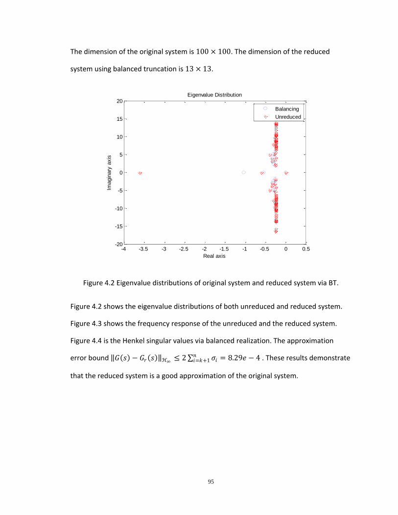
95
The dimension of the original system is 100 × 100. The dimension of the reduced
system using balanced truncation is 13 × 13.
Figure 4.2 Eigenvalue distributions of original system and reduced system via BT.
Figure 4.2 shows the eigenvalue distributions of both unreduced and reduced system.
Figure 4.3 shows the frequency response of the unreduced and the reduced system.
Figure 4.4 is the Henkel singular values via balanced realization. The approximation
error bound 𝐺 𝑠 − 𝐺𝑟 𝑠 ℋ∞≤ 2 𝜍𝑖 = 8.29𝑒 − 4 𝑛
𝑖=𝑘+1 . These results demonstrate
that the reduced system is a good approximation of the original system.
-4 -3.5 -3 -2.5 -2 -1.5 -1 -0.5 0 0.5-20
-15
-10
-5
0
5
10
15
20
Real axis
Imagin
ary
axis
Eigenvalue Distribution
Balancing
Unreduced
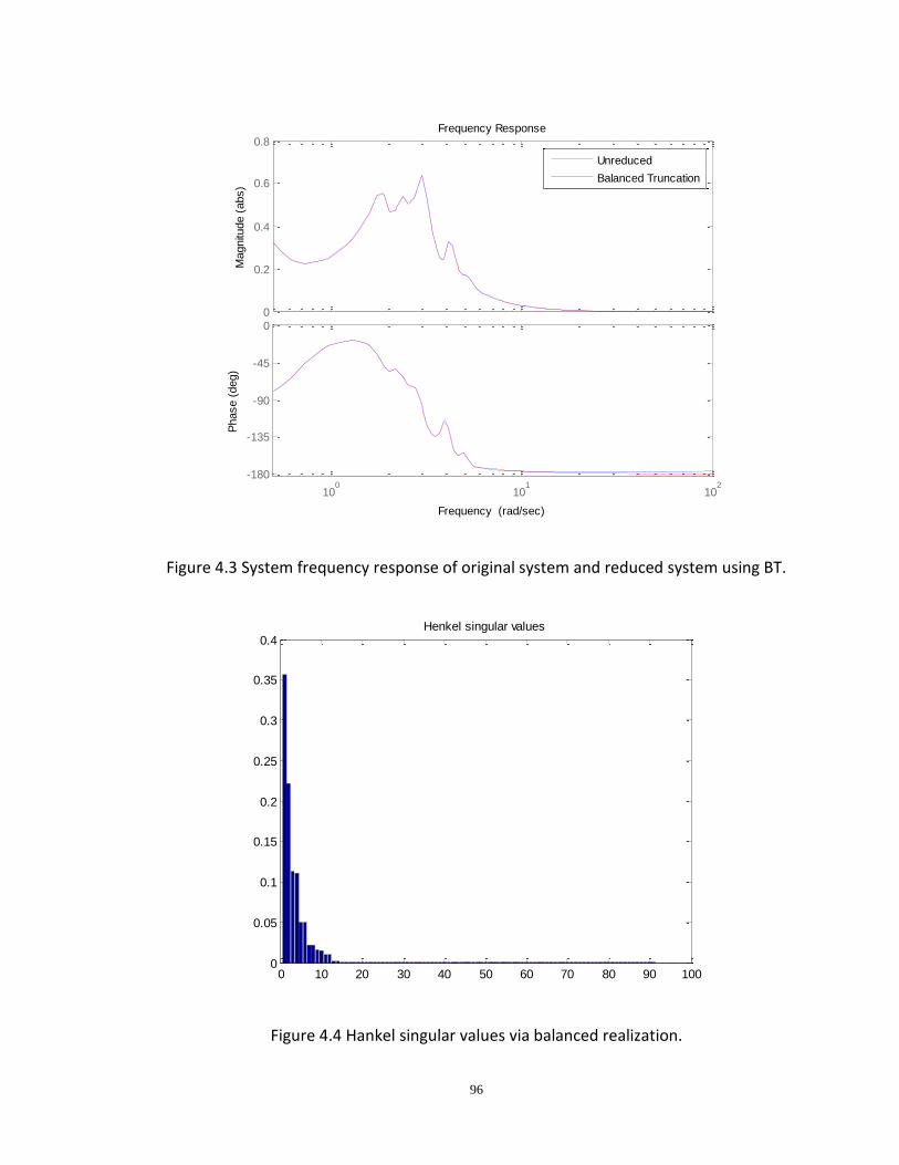
96
Figure 4.3 System frequency response of original system and reduced system using BT.
Figure 4.4 Hankel singular values via balanced realization.
0
0.2
0.4
0.6
0.8
Magnitu
de (
abs)
100
101
102
-180
-135
-90
-45
0
Phase (
deg)
Frequency Response
Frequency (rad/sec)
Unreduced
Balanced Truncation
0 10 20 30 40 50 60 70 80 90 1000
0.05
0.1
0.15
0.2
0.25
0.3
0.35
0.4Henkel singular values
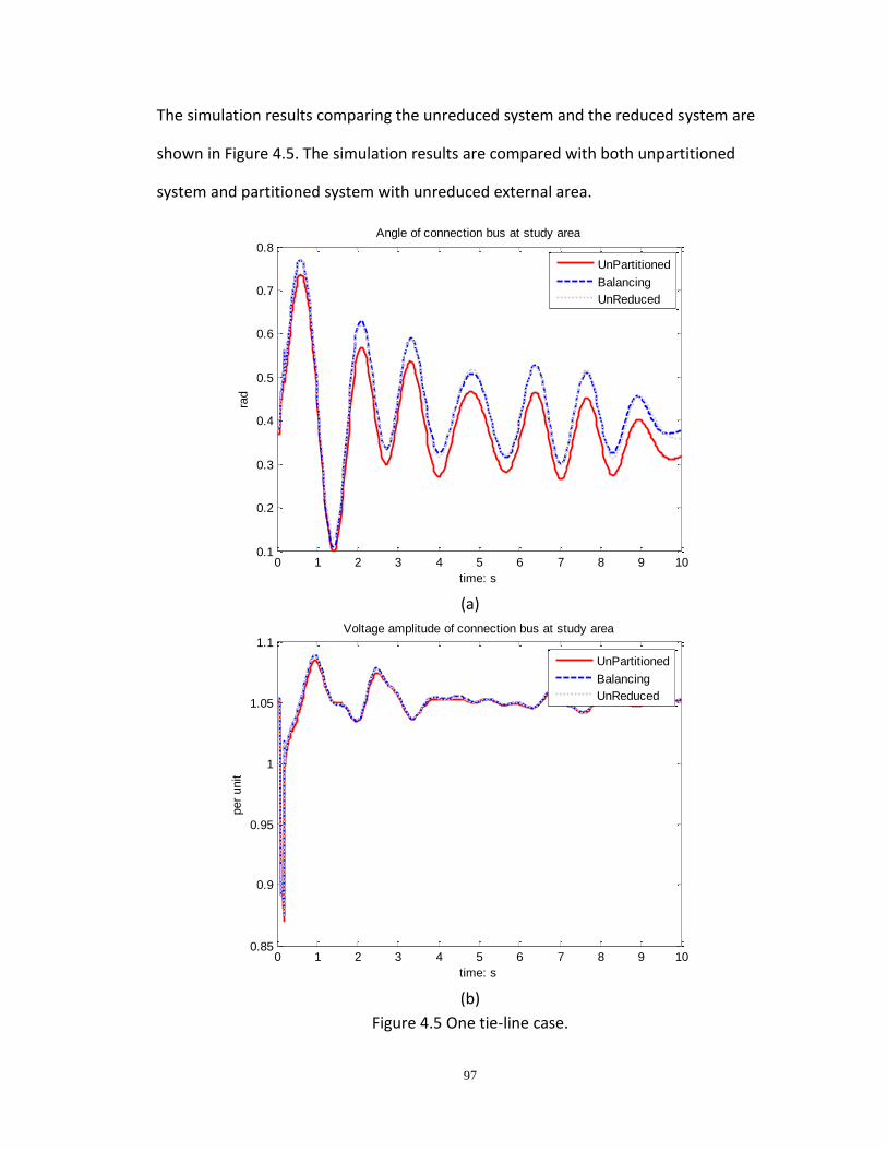
97
The simulation results comparing the unreduced system and the reduced system are
shown in Figure 4.5. The simulation results are compared with both unpartitioned
system and partitioned system with unreduced external area.
(a)
(b)
Figure 4.5 One tie-line case.
0 1 2 3 4 5 6 7 8 9 100.1
0.2
0.3
0.4
0.5
0.6
0.7
0.8
Angle of connection bus at study area
time: s
rad
UnPartitioned
Balancing
UnReduced
0 1 2 3 4 5 6 7 8 9 100.85
0.9
0.95
1
1.05
1.1Voltage amplitude of connection bus at study area
time: s
per
unit
UnPartitioned
Balancing
UnReduced

98
(c)
Figure 4.5 Continued.
4.4.2 Comparison with Krylov subspace
Because the system is connected to the study area through only one tie-line, only one
interpolation point at zero frequency is used (𝜍 = 0) [30].
The dimension of the reduced system is 21*21 using the Krylov subspace method.
Figure 4.6 shows the eigenvalue distributions and Figure 4.7 shows the frequency
response. The reduced model of both methods captures the dominant modes of the
original system. Also, frequency response suggests that Krylov subspace follows the
unreduced system well for low frequencies, but might lose the track for high
frequencies. This is because we use 𝜍 = 0 as the interpolation point.
0 1 2 3 4 5 6 7 8 9 10
0.35
0.4
0.45
0.5
0.55Angle of connection bus at external area
time: s
rad
UnPartitioned
Balancing
Unreduced
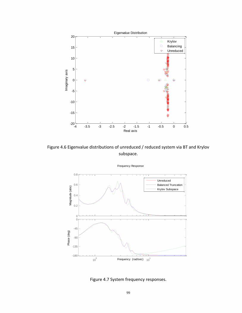
99
Figure 4.6 Eigenvalue distributions of unreduced / reduced system via BT and Krylov
subspace.
Figure 4.7 System frequency responses.
-4 -3.5 -3 -2.5 -2 -1.5 -1 -0.5 0 0.5-20
-15
-10
-5
0
5
10
15
20
Real axis
Imagin
ary
axis
Eigenvalue Distribution
Krylov
Balancing
Unreduced
0
0.2
0.4
0.6
0.8
Magnitu
de (
abs)
100
101
-180
-135
-90
-45
0
Phase (
deg)
Frequency Response
Frequency (rad/sec)
Unreduced
Balanced Truncation
Krylov Subspace
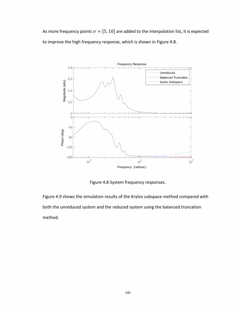
100
As more frequency points 𝜍 = 5, 10 are added to the interpolation list, it is expected
to improve the high frequency response, which is shown in Figure 4.8.
Figure 4.8 System frequency responses.
Figure 4.9 shows the simulation results of the Krylov subspace method compared with
both the unreduced system and the reduced system using the balanced truncation
method.
0
0.2
0.4
0.6
0.8M
agnitu
de (
abs)
100
101
102
-180
-135
-90
-45
0
Phase (
deg)
Frequency Response
Frequency (rad/sec)
Unreduced
Balanced Truncation
krylov Subspace
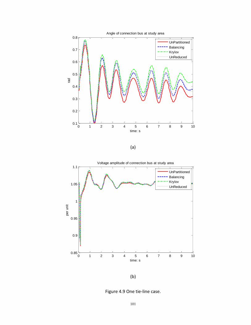
101
(a)
(b)
Figure 4.9 One tie-line case.
0 1 2 3 4 5 6 7 8 9 100.1
0.2
0.3
0.4
0.5
0.6
0.7
0.8
Angle of connection bus at study area
time: s
rad
UnPartitioned
Balancing
Krylov
UnReduced
0 1 2 3 4 5 6 7 8 9 100.85
0.9
0.95
1
1.05
1.1Voltage amplitude of connection bus at study area
time: s
per
unit
UnPartitioned
Balancing
Krylov
UnReduced
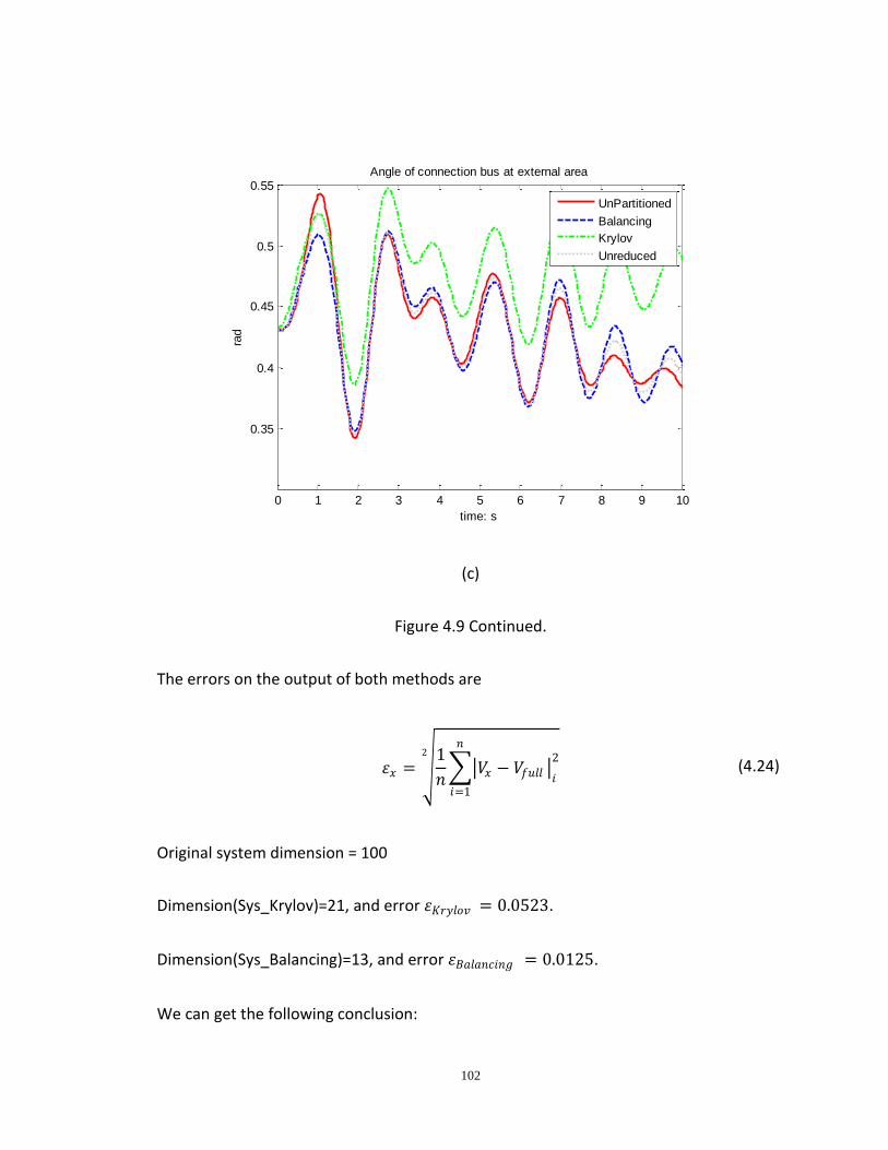
102
(c)
Figure 4.9 Continued.
The errors on the output of both methods are
휀𝑥 = 1
𝑛 𝑉𝑥 − 𝑉𝑓𝑢𝑙𝑙 𝑖
2𝑛
𝑖=1
2
(4.24)
Original system dimension = 100
Dimension(Sys_Krylov)=21, and error 휀𝐾𝑟𝑦𝑙𝑜𝑣 = 0.0523.
Dimension(Sys_Balancing)=13, and error 휀𝐵𝑎𝑙𝑎𝑛𝑐𝑖𝑛𝑔 = 0.0125.
We can get the following conclusion:
0 1 2 3 4 5 6 7 8 9 10
0.35
0.4
0.45
0.5
0.55Angle of connection bus at external area
time: s
rad
UnPartitioned
Balancing
Krylov
Unreduced

103
The balanced truncation method can achieve a better approximation than the Krylov
subspace method while using a smaller ordered system, which represents the direct
input-output relation of the system and eliminates the redundancy in the Krylov
subspace method.
The reduced system preserves most information of the unreduced system regarding the
input-output relation. But partitioning the whole system into study and external area
will sacrifice some accuracy.
4.5 Sensitivity Analysis
Since we perform model reduction on the linearized system model, we now perform
sensitivity analysis to improve the algorithm.
Sensitivity analysis (SA) is the study of how the variation (uncertainty) in the output of a
mathematical model can be apportioned, qualitatively or quantitatively, to different
sources of variation in the input of a model [32].
There are several possible approaches to perform SA, such as local methods, sampling-
based methods, methods based on emulators, screening methods, variance based
methods, and high dimensional model representations, etc. We use local methods for
our problem. Local methods utilize the idea of using the simple derivative of the output
𝑦 with respect to an input factor 𝑥𝑖 , 𝜕𝑦
𝜕𝑥𝑖 𝑥0
, where the subscript 𝑥0 indicates that the
derivative is taken at some fixed point in the space of the input (hence the 'local' in the
name of the class).
In general, the derivative can be obtained either analytically by working on the system
equations or quantitatively by studying the variations of output with respect to the

104
small variations in parameters. In this problem, our goal is to detect the system model
variation, so we choose the quantitative approach to avoid working on a large number
of variables and complex relation between parameter and system model
characterization, and to take advantage of computer programming.
From Figures 4.10 and 4.11, we can see that system (4.22) is more sensitive to machine
angles than bus voltages. It is also worth mentioning that, since the machine angles tend
to change along the same direction, their influences on output variations might cancel
each other out.
Figure 4.10 Sensitivity analysis of machine angles.
0 5 10 15 20 25 30 35 40 45 50-0.1
-0.05
0
0.05
0.1
0.15
0.2
0.25
0.3
0.35
Machine number
the influence of machine angle on system model

105
Figure 4.11 Sensitivity analysis of bus voltages.
We sign the index to each parameter according to the sensitivity analysis and calculate
the aggregated expected variance of the system. When such variance reaches some
preset threshold, we then update the system model.
The importance of such sensitivity study and system model updating is illustrated in the
next section using a three tie-line case.
4.5.1 Simulation results of three tie-line case
In this section, a three tie-line case is studied, in which three tie-lines connect the study
and external areas. The same fault is applied to the system and then is cleared in 0.1 s.
Figure 4.12 shows the singular values of the original unreduced system, through the
balanced truncation method and through the Krylov subspace method.
0 50 100 150-0.1
-0.05
0
0.05
0.1
0.15
Bus Number
the influence of bus voltage on system model
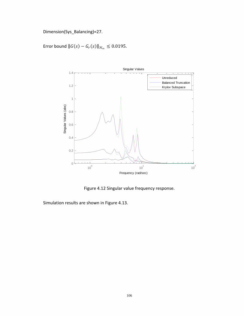
106
Dimension(Sys_Balancing)=27.
Error bound 𝐺 𝑠 − 𝐺𝑟 𝑠 ℋ∞≤ 0.0195.
Figure 4.12 Singular value frequency response.
Simulation results are shown in Figure 4.13.
100
101
102
0
0.2
0.4
0.6
0.8
1
1.2
1.4
Singular Values
Frequency (rad/sec)
Sin
gula
r V
alu
es (
abs)
Unreduced
Balanced Truncation
Krylov Subspace
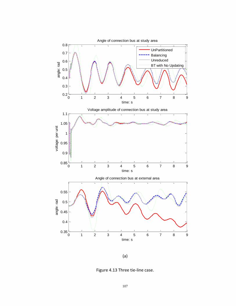
107
(a)
Figure 4.13 Three tie-line case.
0 1 2 3 4 5 6 7 8 90.2
0.3
0.4
0.5
0.6
0.7
0.8
Angle of connection bus at study area
time: s
angle
: ra
d
0 1 2 3 4 5 6 7 8 90.85
0.9
0.95
1
1.05
1.1Voltage amplitude of connection bus at study area
time: s
voltage:
per
unit
0 1 2 3 4 5 6 7 8 90.35
0.4
0.45
0.5
0.55
Angle of connection bus at external area
time: s
angle
: ra
d
UnPartitioned
Balancing
Unreduced
BT with No Updating
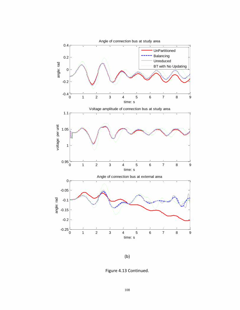
108
(b)
Figure 4.13 Continued.
0 1 2 3 4 5 6 7 8 9-0.4
-0.2
0
0.2
0.4Angle of connection bus at study area
time: s
angle
: ra
d
0 1 2 3 4 5 6 7 8 90.95
1
1.05
1.1Voltage amplitude of connection bus at study area
time: s
voltage:
per
unit
0 1 2 3 4 5 6 7 8 9-0.25
-0.2
-0.15
-0.1
-0.05
0Angle of connection bus at external area
time: s
angle
: ra
d
UnPartitioned
Balancing
Unreduced
BT with No Updating

109
(c)
Figure 4.13 Continued.
0 1 2 3 4 5 6 7 8 9-0.5
0
0.5
1
Angle of connection bus at study area
time: s
angle
: ra
d
0 1 2 3 4 5 6 7 8 90.8
0.85
0.9
0.95
1
1.05
1.1Voltage amplitude of connection bus at study area
time: s
voltage:
per
unit
0 1 2 3 4 5 6 7 8 90.2
0.25
0.3
0.35
0.4Angle of connection bus at external area
time: s
angle
: ra
d
UnPartitioned
Balancing
Unreduced
BT with No Updating
110
4.6 Conclusion
The balanced truncation method is applied to power system model reduction in this
chapter. The emphasis on the input-output connection of the balanced truncation
method helps remove redundant information while preserving the relation between
system input and output. Simulation results prove that the reduced order system via
balanced truncation is a good approximation of the original high order system.
Compared with the Krylov subspace method, it represents a better approximation with
fewer orders. Also, the error of the balanced truncation method is bounded. Since a
linearized system is used, updating the system model based on sensitivity analysis can
improve the performance.
Other readings can be found in [33]-[39].
4.7 References
[1] J. H. Chow, R. Galarza, P. Accari, and W. W. Price, "Inertial and slow coherency
aggregation algorithms for power system dynamic model reduction," IEEE
Transactions on Power Systems, vol. 10, no. 2, pp. 680-685, May 1995.
[2] J. H. Chow, "A nonlinear model reduction formulation for power system slow
coherency and aggregation," in Proceedings of Workshop on Advances in Control
and its Applications, vol. 208, 1996, pp. 282-298.
[3] J. J. Sanchez-Gasca and J. H. Chow, "Power system reduction to simplify the design
of damping controllers for interarea oscillations," IEEE Transactions on Power
Systems, vol. 11, no. 3, pp. 1342-1349, Aug. 1996.
[4] L. Wang, M. Klein, S. Yirga, and P. Kundur, "Dynamic reduction of large power
systems for stability studies," IEEE Transactions on Power Systems, vol. 12, no. 2,
pp. 889-895, May 1997.
111
[5] P. A. Parrilo et al., "Model reduction for analysis of cascading failures in power
systems," in Proceedings of the American Control Conference, vol. 6, San Diego, CA,
1999, pp. 4208-4212.
[6] S.-K. Joo, C.-C. Liu, L. E. Jones, and J.-W. Choe, "Coherency and aggregation
techniques incorporating rotor and voltage dynamics," IEEE Transactions on Power
Systems, vol. 19, no. 2, pp. 1068-1075, May 2004.
[7] Electric Power Research Institute, "Development of dynamic equivalents for
transient stability studies," EPRI, Palo Alto, CA, Tech. Rep. no. EL-456, Project 763,
1977.
[8] N. Nihei and T. Oyama, "A study on decomposition and model reduction for wide
area power system stability assessment," in IEEE Power Engineering Society 1999
Winter Meeting, vol. 1, New York, NY, 1999, pp. 651-654.
[9] H. Kim, G. Jang, and K. Song, "Dynamic reduction of the large-scale power systems
using relation factor," IEEE Transactions on Power Systems, vol. 19, no. 3, pp. 1696-
1699, Aug. 2004.
[10] P. W. Sauer, D. J. LaGesse, S. Ahmed-Zaid, and M. A. Pai, "Reduced order modeling
of interconnected multimachine power systems," IEEE Transactions on Power
Systems, vol. PWRS-2, no. 2, pp. 310-320, May 1987.
[11] D. Chaniotis and M. A. Pai, "Model reduction in power systems using Krylov
subspace methods," IEEE Transactions on Power Systems, vol. 20, no. 2, pp. 888-
894, May 2005.
[12] S. Gugercin and A. C. Antoulas, "A survey of model reduction by balanced
truncation and some new results," International Journal of Control, vol. 77, no. 8,
pp. 748-766, May 2004.
[13] R. Podmore, "Identification of coherent generators for dynamic equivalents," IEEE
Transactions on Power Apparatus and Systems, vol. PAS-97, no. 4, pp. 1344-1354,
July 1978.
[14] S. T. Y. Lee and F. C. Schweppe, "Distance measures and coherency recognition for
transient stability equivalents," IEEE Transactions on Power Apparatus and Systems,
vol. PAS-92, no. 5, pp. 1550-1557, Sep. 1973.
112
[15] M. A. Pai and R. P. Adgaonkar, "Electromechanical distance measure for
decomposition of power systems," Electrical Power & Energy Systems, vol. 6, no. 4,
pp. 249-254, 1984.
[16] B. D. Spalding, H. Yee, and D. B. Goudie, "Coherency recognition for transient
stability studies using singular points," IEEE Transactions on Power Apparatus and
Systems, vol. 96, no. 4, pp. 1368-1375, July 1977.
[17] J. H. Chow, "New algorithms for slow coherency aggregation of large power
systems," in Systems and Control Theory for Power Systems. New York, NY:
Springer, 1995, vol. 64, pp. 95-115.
[18] Y. Ohsawa and M. Hayashi, "Coherency recognition for transient stability
equivalents using Lyapunov function," in 6th Power System Computation
Conference, vol. 2, Aug. 1978, pp. 815-818.
[19] M. H. Haque and A. H. M. A. Rahim, "Identification of coherent generators using
energy function," IEE Proceedings-Generation, Transmission and Distribution, vol.
137, no. 4, pp. 255-260, 1990.
[20] M.-H. Chang and H.-C. Wang, "Novel clustering method for coherency identification
using an artificial neural network," IEEE Transactions on Power Systems, vol. 9, no.
4, pp. 2056-2062, Nov. 1994.
[21] A. I. Zečevid and N. Gačid, "An algorithm for model reduction in large electric power
systems," Mathematical Problems in Engineering, vol. 4, no. 1, pp. 43-58, 1998.
[22] Y. Saad, Iterative Methods for Sparse Linear Systems, 2nd ed. Philadelphia, PA:
Society for Industrial and Applied Mathematics, 2003.
[23] A. Laub, M. Heath, C. Paige, and R. Ward, "Computation of system balancing
transformations and other applications of simultaneous diagonalization
algorithms," IEEE Transactions on Automatic Control, vol. 32, no. 2, pp. 115-122,
Feb. 1987.
[24] B. Moore, "Principal component analysis in linear systems: Controllability,
observability, and model reduction," IEEE Transactions on Automatic Control, vol.
26, no. 1, pp. 17-32, Feb. 1981.
113
[25] K. Glover, "All optimal Hankel-norm approximations of linear multivariable systems
and their L∞-error bounds," International Journal of Control, vol. 39, no. 6, pp.
1115-1193, 1984.
[26] S. Lall, J. E. Marsden, and S. Glavaski, "A subspace approach to balanced truncation
for model reduction of nonlinear control systems," International Journal of Robust
and Nonlinear Control, vol. 12, no. 6, pp. 519-535, 2002.
[27] S. Lall and C. Beck, "Error bounds for balanced model reduction of linear time-
varying systems," IEEE Transactions on Automatic Control, vol. 48, no. 6, pp. 946-
956, 2003.
[28] H. Sandberg and A. Rantzer, "Balanced truncation of linear time-varying systems,"
IEEE Transactions on Automatic Control, vol. 49, no. 2, pp. 217-229, Feb. 2004.
[29] P. W. Sauer and M. A. Pai, Power System Dynamics and Stability. Upper Saddle
River, NJ: Prentice Hall, 1998.
[30] D. Chaniotis, "Krylov subspace methods in power system studies," Ph.D.
dissertation, University of Illinois at Urbana-Champaign, 2001.
[31] J. Chow and G. Rogers, "Power Systems Toolbox." [Online]. Available:
http://www.eagle.ca/~cherry/pst.htm.
[32] A. Saltelli et al., Global Sensitivity Analysis: The Primer. Hoboken, NJ: Wiley-
Interscience, 2008.
[33] S.-C. Wang and P.-H. Huang, "A fuzzy method for power system model reduction,"
in 2004 IEEE International Conference on Fuzzy Systems, vol. 2, Budapest, Hungary,
2004, pp. 891-894.
[34] V. Mehrmann and T. Stykel, "Balanced truncation model reduction for large-scale
systems in descriptor form," in Dimension Reduction of Large-scale Systems:
Proceedings of a Workshop, Oberwolfach, Germany, 2003, pp. 83-115.
[35] "Model reduction," Fall 2004. [Online]. Available: http://web.mit.edu/mor/.
[36] E. J. Grimme, "Krylov projection methods for model reduction," Ph.D. dissertation,
University of Illinois at Urbana-Champaign, 1997.
114
[37] H. Sandberg and A. Rantzer, "Balanced truncation of linear time-varying systems,"
IEEE Transactions on Automatic Control, vol. 49, no. 2, pp. 217-229, Feb. 2004.
[38] S. Lall and C. Beck, "Error bounds for balanced model reduction of linear time-
varying systems," IEEE Transactions on Automatic Control, vol. 48, no. 6, pp. 946-
956, 2003.
[39] I. Kamwa, R. Grondin, J. Dickinson, and S. Fortin, "A minimal realization approach to
reduced-order modelling and modal analysis for power system response signals,"
IEEE Transactions on Power Systems, vol. 8, no. 3, pp. 1020-1029, Aug. 1993.
115
CHAPTER 5
CONCLUSION
5.1 Summary of the Main Results
In the operation, simulation and control of power systems, the use of real-time data
relating to system states can yield precise forecasts and enable robust active control. In
this dissertation we developed “data enhanced” models and filters for large-scale power
systems to better understand the dynamic nature of power system behavior and to
have good knowledge of the dynamic states of the system. The work focused on three
areas: load modeling, nonlinear filtering for machine states and parameters estimation,
and order reduction.
Load modeling has gained more attention in recent years to catch up with the
continuous changes in the electricity industry, which have forced changes in the
transmission system such that power systems now operate closer to their limits. We
developed the automatic load identification procedure not only to model the load but
also to update load parameters in real time as measurement data are received. The
procedure here utilizes the normal operational data without big disturbances or step
test. The Levenberg-Marquardt algorithm is proved to be a good tool for parameter
estimation in such situations. Since the information in normal operational data is easily
annihilated by noise, the criteria to judge the parameter estimatability from noisy data
are originally proposed and tested.

116
A state-of-the-art nonlinear filtering technique, particle filters (PFs), was first introduced
to perform synchronous machine state/parameter estimation. The tremendous
advantage of this technique is that it includes uncertainties to make the model time
variable and hence can reflect the underlying system disturbances and uncertainties,
resulting in better knowledge for active control design. With dynamic data available
from phasor measurement units (PMU), machine parameters can now be validated and
corrected online. The PFs method removes the limitation of local linearization and
Gaussian distribution assumption and has the advantage of processing data sequentially
as it arrives, thereby enabling rapid adaptation to changing signal. It was also shown that
the performance of PFs can be further improved by using more particles, or by applying
smoothing techniques.
Model reduction is an important issue in reducing the computational cost of the data-
driven electrical power system analysis. The balanced truncation method was
introduced for the first time for use in power system model reduction. The supreme
advantage of balanced truncation is that it emphasizes input-output, and it removes the
redundant information while preserving the relation between system input and output,
which is ideal for the analysis of interconnected power systems. Simulation results
showed that balanced truncation represents a better approximation with fewer orders
than the Krylov subspace method. Also, asymptotic stability is preserved, and the error
is bounded. Since a linearized system is used, updating the system model based on
sensitivity analysis can improve the performance.
Overall, in this dissertation we have shown that more realistic models with time-varying
parameters can be identified, more accurate state/parameter can be estimated with

117
dynamic data available, and the order of large-scale power systems can be reduced to
ease the complexity of “data-enhanced” analysis.
5.2 Future Research
The work of load modeling can be continued by making a connection between
measurement-based models and component-based models, so that load forecast
information can be integrated and studied in advance. The work of nonlinear filtering
can be continued by applying it to other power system problems. Also, the importance
density can be tailored to specific problems to achieve better performance. The work of
model reduction can be continued by finding the connections with coherency analysis
and studying the impact of partitioning.
Besides all the above, future research can be carried on by applying the results with real
PMU data. The problems associated with this include, but are not limited to, data
filtering and pre-processing, and bad data detection.

118
AUTHOR’S BIOGRAPHY
Shanshan Liu was born in Yangzhou, P. R. China, on November 17, 1978. She received
her bachelor’s degree in engineering and master’s degree in electrical engineering from
Tsinghua University in July 2000 and July 2002, respectively. She joined the Power and
Energy Systems group at the University of Illinois at Urbana-Champaign in 2002. She is a
member of the IEEE Power Electronics Society / Power Engineering Society Joint
Students Chapter. Her research interests include power system analysis, modeling and
simulation.