University of Nebraska - LincolnDigitalCommons@University of Nebraska - Lincoln

Journal of Actuarial Practice 1993-2006 Finance Department

2002

Dynamic Funding and Investment Strategy forDefined Benefit Pension Schemes: A ModelIncorporating Asset-Liability Matching CriteriaShih-Chieh ChangNational Chengchi University, bchang@nccu.edu.tw

Cheng-Hsien TsaiNational Chengchi University, ctsai@nccu.edu.tw

Chia-Jung TienInsurance Institute of Republic of China, tarisa.tien@msa.hinet.net

Chang-Ye TuNational Chengchi University, tu@cercom.iam.ntu.edu.tw

Follow this and additional works at: http://digitalcommons.unl.edu/joap

Part of the Accounting Commons, Business Administration, Management, and OperationsCommons, Corporate Finance Commons, Finance and Financial Management Commons, InsuranceCommons, and the Management Sciences and Quantitative Methods Commons

This Article is brought to you for free and open access by the Finance Department at DigitalCommons@University of Nebraska - Lincoln. It has beenaccepted for inclusion in Journal of Actuarial Practice 1993-2006 by an authorized administrator of DigitalCommons@University of Nebraska -Lincoln.

Chang, Shih-Chieh; Tsai, Cheng-Hsien; Tien, Chia-Jung; and Tu, Chang-Ye, "Dynamic Funding and Investment Strategy for DefinedBenefit Pension Schemes: A Model Incorporating Asset-Liability Matching Criteria" (2002). Journal of Actuarial Practice 1993-2006.40.http://digitalcommons.unl.edu/joap/40

Journal of Actuarial Practice Vol. 10,2002

Dynamic Funding and Investment Strategy for Defined Benefit Pension Schemes: A Model Incorporating Asset-Liability Matching Criteria

Shih-Chieh Chang,* Cheng-Hsien Tsai,t Chia-Jung Tien,* and Chang-Ye Tu§

Abstract

This paper studies the dynamic funding policy and investment strategy for defined benefit pension plans using one of the most comprehensive dynamic

* Shih-Clueh Chang, Ph.D., is a professor in the Department of Risk Management and Insurance at National Chengchi University, Taipei, Taiwan, R.O.C. Dr. Chang received his B.Sc. in mathematics from National Taiwan University and his Ph.D. in statistics from University of Wisconsin, Madison. His research interests are stochastic models for actuarial science and financial market in Taiwan.

Dr. Chang's address is: Department of Risk Management and Insurance, College of Commerce, National Chengchi University, 64 Sec. 2 Chinan Rd, Taipei, TAIWAN, R.O.C. Internet address: bchang@nccu.edu.tw

tCheng-Hsien TSai, Ph.D., is an assistant professor in the Department of Risk Man­agement and Insurance at National Chengchi University. Dr. Tsai received his bachelor's degree in finance from National Taiwan University, MBA in finance from Carnegie Mellon University, and Ph.D. in insurance from Georgia State University. His research interests are mainiy in insurance finance and solvency regulation of insurers.

Dr. Tsai's address is: Department of Risk Management and Insurance, College of Commerce, National Chengchi University, 64 Sec. 2 Chinan Rd, Taipei, TAIWAN, R.O.C. Internet address: ctsai@nccu.edu.tw

* Chia-Jung Tien is a project researcher in the Insurance Institute of Republic of China. She received her bachelor's degree in mathematics from National Taiwan University and MBA in insurance from National Chengchi University.

Ms. Tien's address is: Department of Risk Management and Insurance, College of Commerce, National Chengchi University, 64 Sec. 2 Chinan Rd, Taipei, TAIWAN, R.O.C. Internet address: tarisa.tien@msa.hinet.net

§Chang-Ye Tu is a research assistant in the Department of Risk Management and Insurance at National Chengchi University. He received both his bachelor's degree in civil engineering and MS degree in applied mechanics from National Taiwan University.

Mr. Tu's address is: Department of Risk Management and Insurance, College of Com­merce, National Chengchi University, 64 Sec. 2 Chinan Rd, Taipei, TAIWAN, R.O.C. In­ternet address: tu@cercom.iam.ntu.edu.tw

131

132 Journal of Actuarial Practice, Vol. 10, 2002

pension models to date. The model includes three investable assets: one risk­free and two risky. The optimal plan decisions are formulated as a stochastic control problem that is solved using dynamic programming. The objective function uses performance measures to take into account the stability and solvency of the plan. The model is then applied to a Taiwanese pension.

Key words and phrases: optimal contribution, asset allocation, dynamic pro­gramming, performance measure

1 Introduction

Although most pension liabilities are long-term in nature, traditional defined benefit pension plan management is based on one-period as­sumptions.1 The pension plan manager seeks an optimal investment decision for the next period, based on the plan's current experience, cur­rent market conditions, and expectations about future contributions, returns, and risks. Such a short-sighted mechanism has two drawbacks: (i) the accumulation of a sequence of single-period optimal decisions across each of n periods may not be optimal for the n periods taken as a whole; and (ii) single-period decisions have difficulties in dealing with the investment and funding sides of a pension plan because the interac­tion between investments and funding appears only in the multi-period setting.

An important tool that can be used to assist plan managers in devel­oping optimal funding policies over many periods is stochastic optimal control theory. This theory can be used to solve long-term financial planning problems through global optimization across periods instead of local optimization within a period.

Control theory has been developed by engineers since the 1930s. Its applications to economics emerged in the 1950s. [See Petit (1990) for more on this.] Several authors, including Samuelson (1969), Mer­ton (1971,1990), Brennan and Schwartz (1982), Karatzas et aI., (1986), Brennan, Schwartz, and Lagnado (1997), Boyle and Yang (1997), Bren­nan and Schwartz (1998), and Sorensen (1999), have studied optimal consumption and investment problems using control theory. Although the popularity of stochastic control theory was hindered by its inher-

1 Traditional pension management usually employs a mean-variance approach. Sharpe (1991) describes the mean-variance approach as a highly parsimonious char­acterization of investors' goals, employing a myopic view (Le., one period at a time) and focusing on only two aspects of the probability distribution of possible returns over that period.

Chang: Dynamic Funding and Investment Strategy 133

ent complexity, it is becoming more popular today due to the ready availability of high-speed computers.

The application of control theory to pension plan management star­ted with O'Brien (1986, 1987) who constructed a stochastic model for the pension plan and studied the optimal funding poliCies for target funding ratios. Cairns (1995, 1996, 2000) introduced asset allocation into the control process to study the optimal funding and investment strategies needed to minimize certain quadratic loss functions. Chang (1999, 2000) applied their methods to a real pension plan in Taiwan us­ing service tables and stochastic asset returns to numerically solve for optimal funding poliCies over various time horizons. Applications of control theory to other actuarial problems can be seen in Runggaldier (1998) and ScMI (1998). Runggaldier reviews the concepts and solu­tion methods, while ScMI focuses on the dynamic programming for piecewise deterministic Markov processes.

In this paper we construct one of the most comprehensive dynamic models of a pension plan to date, numerically solve the stochastic con­trol problem, and provide illustrations of the optimal investment and funding strategies. Compared to Cairns (1995, 1996, 2000), we have a richer set of liability dynamics, and we have included risk-free as well as risky assets. Compared with Chang (1999, 2000), we consider not only funding poliCies, but also asset allocations. In addition we consider more risk factors for invested assets. Furthermore, our performance measures (also called loss functions) take into account the stability of contributions and the security (the funding ratio) of the pension plan.

The features of our models are summarized as follows:

1. The dynamics of the plan's demography can be explicitly incorpo­rated into investment decisions under different evaluation time horizons.

2. The optimal funding and investment strategies of the plan can be formalized with speCific risk performance measures through a computerized system.

3. The contribution risk and solvency risk associated with any fund­ing policy and investment strategy can be assessed given any eval­uation horizon.

The paper is organized as follo~s. Section 2 describes the model (Le., the basic framework, the dynamics of invested assets, and perfor­mance measures used) of the proposed dynamic optimization scheme.

134 Journal of Actuarial Practice, Vol. 10, 2002

Section 3 develops the solution to the optimal equation. Section 4 pro­vides a practical example to illustrate the usefulness of the theory pre­sented. A summary and closing comments are given in Section 5.

2 The Model

In this section, we formulate the funding and investment decisions of pension funds as an stochastic optimal control problem. These deci­sions are modeled through a continuous-time stochastic process over a specific evaluation time horizon.

2.1 The Basic Framework

The following notation is used for the various stochastic processes2

used in the paper:

T = Management's planning horizon;

Jt = Plan's history up to time t;

F (t) = Total assets of the pension plan at time t excluding any con­tributions made at time t;

db (t, F) = Rate of investment return in (t, t + dt);

cet) = Contributions at time t;

B(t) = Retirement benefit payment rate at time t;

O'B = Volatility of B(t);

Zi(t) = Wiener processes (i E {NC,B, W) at time t;

AL(t) = Total plan accrued liabilities at time t;

r' = Valuation rate for accrued liabilities;

NC(t) = Normal cost rate at time t;

Wet) = Reduction rate in retirement liability at time t due to with­drawal payment;3

2Throughout this paper we assume that all stochastic processes are defined on ap­propriate probability spaces.

3Because death benefits are not currently included in the Taiwanese Labor Standard Law and withdrawal benefits are not paid from the accumulated penSion fund, we con­sider only the retirement benefits payments and the reduced withdrawal liability in this paper.

Chang: Dynamic Funding and Investment Strategy

(5NC = Volatility of NC(t); and

(5w = Volatility of W(t).

135

The (5S are assumed to be constants. The term rate, as used with respect to C (t), NC (t), B (t), and W (t), refers to the amount paid in an infinites­imal time interval. For example, C(t)dt is the amount contributed in (t, t + dt).

The funding level F(t) and accrued liabilities AL(t) are described by the following stochastic differential equations:

dF(t) = F(t)d8(t,F) + C(t)dt - B(t)dt + (5B dZB(t), (1)

dAL(t) = (AL(t)r' + NC(t) - B(t) - W(t))dt + (5NC dZNc(t)

+ (5B dZB(t) + (5w dZw(t). (2)

2.2 The Dynamics of Invested Assets

We assume three types of assets are available to the penSion plan: cash, stocks, and consol bonds.4 The proportion of the pension funds invested in stocks, consol bonds, and cash at time t is denoted by P (t) = (a(t), b(t), c(t)), where

a(t) + b(t) + c(t) = 1.

Following Brennan, Schwartz, and Lagnado (1997), we model the in­stantaneous rate of return on the stock portfolio dS (t) / S (t), the short rate r(t), and the long rate l(t), as the following joint stochastic pro­cess:

dS(t) S(t) = f.1sdt + (5sdZs(t),

dr(t) = f.1rdt + (5rdZr (t),

dl(t) = f.11dt + (51dZl(t),

(3)

(4)

(5)

where the subscripts S, r, l refer to stocks, short rate, and long rate, respectively, f.1i and (5i (i E {S, r, l}) are constant parameters and dZi (i E {S, r, l}) are increments to Wiener processes.

We note that the price of a consol bond, Be (t), is inversely propor­tional to its yield and the total return of a consol bond is the sum of

4Consol bonds are bonds with infinite time to maturity, i.e., they never mature.

136 Journal of Actuarial Practice, Vol. 10, 2002

the yield and the price change. Also, from a simple application of Ito's lemma, the instantaneous total return on the consol bond can be proved to be:

dBc(t) (PI a}) Ul Bc(t) + l(t)dt = l(t) - l(t) + l(t)2 dt - l(t) dZI(t). (6)

The investment return of the pension plan between time t and t + dt, d8(t,F), can be formulated as:

d8(t,F) = a(t) ~~~) +b(t) (~c(~~) + l(t)dt) +(l-a(t)-b(t))r(t)dt.

(7) Hence, the instantaneous changes in the pension's assets in equation (1) can be rewritten as

dF(t) = F(t) [a(t)Ps + b(t) (l- l~:) + l~l:)) + (1 - a(t) - b(t))r(t) ] dt

+ (C(t) - B(t))dt + F(t)a(t)usdZs(t) - F(t)b(t) l~) dZI(t)

+ uBdZB(t). (8)

The dynamics of the pension plan for the fund and the accrued liabili­ties can then be jointly written as:

( dF(t) ) dAL(t) == dX(t) = Px(t)dt + ux(t)d~(t), (9)

where

( ) = ([aps + b(l- Pill + ul Il2) + (1 - a - b)r]F + C - B)

px t Ai . r' + NC _ B _ W '

ux(t) = (Faus -Fbut/l UB 0 0 ) , o 0 UB UNC Uw

and d~ = (dZs, dZl, dZB, dZNC, dZw) T is a five dimensional standard Wiener process with covariance matrix [Uij]. We adopt the notation USI to denote the covariance between Wiener processes Zs and Zl; other covariances are represented similarly.

Chang: Dynamic Funding and Investment Strategy 137

Note: In the definition of Jix(t) and ux(t) above the function def­initions are abbreviated by dropping (t) so that, for example, F(t) is written as F and a(t) is written as a. When no confusion arises, (t) and subscripts t or T will be omitted. This convention is used throughout the rest of this paper.

2.3 Performance Measures

A good performance measure should consider the two most impor­tant factors in pension plan valuations: (i) the contribution rate risk (i.e., level of funding deficiency), which is the difference between nor­mal costs and contributions; and (ii) the level of unfunded liabilities, which is the difference between accrued liabilities and assets. The level of funding deficiency affects the stability of the plan, while the level of unfunded liabilities affects the solvency of the plan. Following Haber­man and Sung (1994), we design our performance measure (also called a loss function) to take into account the contribution rate and solvency risks to give:

L(t,X, {C,P}) = (NC(t) - C(t))z + k(17AL(t) -F(t))z, (10)

where k is a constant chosen subjectively by the pension fund manager to adjust for the difference in size between the contribution rate risk and the solvency risk, and 17 is the target funding ratio. The parameter k reflects the relative importance of matching contributions with normal costs and matching plan assets with accrued liabilities.

3 Thp Optimal Equation

Assume first that the performance measure L(t,X, {C,P}) is dis­counted continuously by a constant rate p. If we let B [X T, T] be a func­tion measuring the loss associated with the state of the pension plan at the end of period, then the problem of choosing the optimal asset allocation and funding policy for a fixed evaluation time horizon T can be formulated as:

inf{J: e-ptL(t, X, {C,P} )dt + B[XT, Tn,

subject to the asset and liability dynamics speCified in equations (1) and (2), respectively. Furthermore, we have C ~ 0, a, b, C E R, and F(t) ~ 0. Define

138 Journal of Actuarial Practice, Vol. 10, 2002

J(s, X, {C, P}) = lEs,x[ f: e-pt L(t, X, {C, P} )dt + B[XT, T] Ifs] (11)

where lEs,x represents the expectation conditioned on being in the state X at time s, given information fS. As X is assumed to follow a time­homogeneous Markov process, only the information at s is needed (in­formation before time s can be ignored).

Let us assume that there exit optimal strategies {C*, P*} that form a set of admissible control functions that minimize equation (11), i.e.,

I(s,X) = inf J(s,X,{C,P}) =J(s,X,{C*,P*}). (C,P)

Then by the principle of optimality [Bellman (1957)], we can express the Bellman-Dreyfus fundamental equation of optimality as

inf {[l(l( -B + C - (-1 + a + b)Fy + bFl + aFJis) - bFJiI) + bFa}] l~ lp (C,P)

+ (-B + NC - W + y' AL)IAL

2 2 2 1 + (O"B + O"NC + O"w + 2 O"NCO"WO"NC,W + 2 O"NCO"BO"NC,B + 2 O"WO"BO"WB) Z-lAL,AL

+ lp,F(lO"i + (O"NcCalO"sO"NC,S - bO"[O"NC,dF + O"w(alO"sO"sw - bO"[O"WI))

+ O"B(lO"NCO"NC,B + aFlO"sO"SB + lO"WO"WB - bFO"[O"lB))

+ e-PS((NC - C)2 + keF -I1AL)2)

+ [l20"i + (b20"l + alO"s(alO"s - 2bO"[O"sd)F2

1 + 2FlO"B(alO"sO"SB - bO"[O"lB)] 2t2lp,F} + Is = 0 (12)

where the subscripts of the I denote partial derivatives, i.e., Is = oI/os, h,F = 02 I / oF2, h,AL = 02 II oFoAL, etc. Taking the partial derivatives with respect to C and P and using the boundary condition I(T,X) B[X, T], we obtain from the first order condition that:

C* = NC-e Ps lp/2 (13)

1 2 a* = l 2 2 [lIF(l( -y + l) - JidO"SO"SI + hO"SO"I O"SI

F lp,FO"sO"I(-1 + O"SI)

+ lO"I (lp (-y + Jis) + O"s (h,FO"B (O"SB - O"S[O"IB)

+ lprCO"NCO"NC,S + O"wO"SW - O"NCO"NC,IO"SI + O"BO"SB

- O"WO"SIO"WI - O"BO"S[O"lB))] (14)

Chang: Dynamic Funding and Investment Strategy

1 b* = 2 2 [lh(-r+J.1s)aW·SI

Fh,F(J"S(J"1 (-1 + (J"SI)

+ (J"s(h(-r1 2 + 13 -1J.11 + (J"?) + l(J"I(IF,F(J"B((J"SWSB - (J"IB)

- h,Ad(J"N(J"NC,1 - (J"NC(J"NC,S(J"SI - (J"W(J"SW(J"SI

139

- (J"B(J"SWSB + (J"W(J"WI + (J"B(J"IB))] (15)

The Hamilton-Jacobi-Bellman equation (Fleming and Rishel, 1975) is:

o = Is + lAd - B + NC - W + ALr')

1 2 2 2 + "2 I AL,Ad (J" B + (J" NC + (J" W + 2 (J"NC (J"w (J"NC, W

+ 2 (J"W(J"B(J"WB + 2 (J"NC(J"B(J"NC,B)

I} AL + 21 ('1 2) ((J"Nd(J"NC,1 - (J"NC,S(J"Sz)

F,F - + (J"SI

+ (J"w(-(J"SW(J"SI + (J"wz) + (J"B(-(J"SWSB + (J"/B))2

I},AL((J"NC(J"NC,S + (J"w(J"SW + (J"B(J"SB)2

2h,F

IplFAdr - J.1S)((J"NC(J"NCS + (J"w(J"sw + (J"B(J"SB) + ' , h,F(J"S

1 2 2 lplp,Ad(J"s(l2(-r+l)-1J.11+(J"?) --2h,F(J"B(-1 + (J"SB) + 11 (1 2)

F,F(J"s(J"1 - + (J"SI

+ 1( -r + J.1s ) (J"WSI)((J"Nd -(J"NC,1 + (J"NC,S(J"SI)

+ (J"w((J"SW(J"SI - (J"WI) + (J"B((J"SWSB - (J"IB))

h AL(J"B + ' 2 ((J"Nd -(J"NC 1+ (J"NC S(J"SI) + (J"w((J"SW(J"SI - (J"WI) (-1 + (J"SI) "

+ (J"B((J"SI(J"SB - (J"IB))((J"SI(J"SB - (J"WB) + lp,AL(J"B(J"Nd(J"NC,B - (J"NC,S(J"SB)

+ lp,AL(J"B( -(J"B( -1 + (J"§B) + (J"w( -(J"SW(J"SB + (J"WB))

I}((J"s(l((r -lH + J.1z) - (J"?) + l(r - J.1S)(J"I(J"SI)2 + 222 2 F lp ,F (J" S (J"l (-1 + (J" S I)

1 ( )12 I}(r-J.1s)2 IF,Fd(-(J"sWsB+(J"/B)2 - -e ps F - 2 + 2

4 2h,F(J"s 2 (-1 + (J"SI)

( 2 h(J"B((J"s(l2(-r+l)-1J.11+(J"?) +ke -ps)(F-IJAL) + 1 (1 2)

(J"S(J"l - + (J"SI

+ l(-r + J.1S)(J"WSz) ((J"SWSB - (J"lB)

1 - -lp((B - NC - Fr)(J"s + (-r + J.1s ) (J"B(J"SB ).

(J"s (16)

140 Journal of Actuarial Practice, Vol. 10, 2002

The function (C*, P*) is our candidate for the optimal strategy. Be­cause I (s, X) is unknown, the description is incomplete. We therefore have to guess a solution for 1(s, X) that has finite number of parame­ters, and then use the partial differential equation (16) to identify its parameters. Because our loss function is quadratic, our guess is:

I[s,X] = xt<l>X + 'I'tx + d(s), 0 s ssT.

where d(s) depends only on s, and

and

Substituting <1>, '1', and d(s) into the ordinary system of differential equations and noting that the optimal strategy must hold for all (s, X), we can solve for the coefficient matrices <1>, '1', and d(s) in I[s,X] by checking the coefficients in equations for F2, FAL, AL2, F,AL, and the constant term. The boundary condition is 1(T, X) = B[X, T] = 0, Le., adT) = a2(T) = a3(T) = bdT) = b2(T) = d(T) = 0, because the plan manager who adopts this optimal strategy must be able to match contri­butions with the normal costs and match assets with accrued liabilities at the end of the evaluation period.

After inspecting the formulas for a, b, and C, we find that we need only to compute h, h,p, and h,AL via the solution of ads), a2(s), and br (s). The system of differential equations involving a 1 (s), a2 (s), and br (s) (with (s) removed for convenience) is as follows:

0= l2(r - ps)2alal - 2l(r - ps)crscrz(l2(-r + l) -lpz + crl)crSZal

+ crl (l2 ((r - l)l + pz)2 a1 + crz4al + lcrl (-kle- Ps

- 2((2r -l)l + PZ)al + lePsai -la~ + lcrlz(ke- PS

+ 2ral - ePs ai + a~))) (17)

0= 2(l2(r - ps)2crla2 - 2l(r - ps)crscrz(l2(-r + l) -lpz + crl)crSZa2

+ crl(l2((r -l)l + pz)2 a2 + crz4a2 + lcrl(kll1e-Ps

+ (-2pz + l( -3r + 2l- r' + ePS al))a2

-laz -lcr§z(kl1e-PS) + (r - r' - ePS al)a2 + az)))) (18)

Chang: Dynamic Funding and Investment Strategy 141

0= 12(r -I1S)2 a ibl + 2l(r -I1S)CTSCTl(lCTl((CTNd-CTNC,S + CTNC,lCTSl)

+ CTW(-CTSW + CTSWWz))a2 - CTB(CTSB - CTSlCTlB)(al + a2)

+ (l((r -1)l + Ill) - CTl)CTSlb 1)

+ CT§(2l2(l(-r + l) -11z)CTl((CTNd-CTNC,1 + CTNC,SCTSl)

+ CTW(CTSWCTSI - CTWl))a2

+ CTB(CTSWSB - CTlB)(al + a2)) + 21CTl((CTNd-CTNC,1 + CTNC,SCTSl)

+ CTW(CTSWCTSI - CTWl))a2 + CTB(CTSWSB - CTlB)(al + a2))

+ l2((r -l)1 + 111)2bl + CT(b l

+ lCTl(-2(B - NC + W)l(-l + CT§I)a2

+ (-2111 + 1( -3r + 21 + rCT§I))br - l( -1 + CT§I)al (2B - 2NC

+ ePsbr) + 1(-1 + CT§I)b~)). (19)

Numerical methods can now be used to solve the above system of differential equations for <1>, 'Y and d in order to obtain the optimal strat­egy C*, P* for t E [0, T]). A Mathematica®subroutine that implements the sophisticated implicit Adams and Gear formulae with higher orders is used to solve the system of differential equations numerically.

4 An Illustration

We apply the results in Sections 2 and 3 to a defined benefit pension plan sponsored be a Taiwanese semi-conductor and electronic com­pany. According to the Labor Standard Law enacted by the Taiwanese government in 1984, each employer is required to contribute from 2% to 15% of its employees' pensionable payroll to a government-managed trust fund. This trust fund is guaranteed a minimum return by the Tai­wanese government. This mandatory pension plan is a defined benefit scheme in which a participant's retirement benefit is based on the par­ticipant's length of service and final salary. Although the pension plan has minimum guaranteed returns from the government, the plan is still subject to an insolvency risk because the contributions coupled with the investment returns may not be able to match the benefit payments.

The Taiwanese company's pension plan covers 2,768 members with initial assets of 254 million NT dollars and an accrued liability of 380 million NT dollars. We use the open group with size-constrained as­sumption to project the evolution of the plan's workforce (Winklevoss, 1993). The total number of employees is assumed to remain unchanged, i.e., each departing employee is immediately replaced by a new em-

142 Journal of Actuarial Practice, Vol. 10, 2002

ployee. The plan's service table is given in Tables Al and A2 in the appendix. 5 Table A3 shows the assumptions made for new entrants. The entry age normal cost method (Anderson, 1992) is used to deter­mine accrued liabilities, normal costs, and benefit retirement benefits.

The retirement benefit, B(t), is formulated according to the current Labor Standard Law for the private pension plans in Taiwan. This law stipulates that the retirement benefit can only be paid as lump-sum pay­ment to the retiree. The retirement benefit for a qualified plan member, B(t), can be written as the accumulated service credits multiple by the average final six-month salary. Each plan member receives two service credits each year of service for the first fifteen years of service and one service credit each year after fifteen years of service, up to a maximum of forty-five service credits.

Suppose an active plan member j entered the plan at age e j and is currently age Xj at with annual salary of S(j). If the annual salary growth rate is set at 3%, then the projected retirement benefit, RBEN(}) , can be written as

RBEN{J) _ e . {2X S(}) (1.03)60-xj if 60 - eJ· :::; 15

- S(j)(1.03)60-xj xmin(xe +15,45) if60-ej~15

Let 'R t denote the set of active plan members who retire at time t and W t denote the set of active plan members who withdraw at time t. The aggregated retirement benefit payments and reduced retirement' liability payments at t, respectively, for the plan are given by:

B(t) = I RBEN(}) and JERt

W(t) = I RBEN(}). JEWt

For practical reasons, continuous time processes are simulated at weekly intervals. Salaries are assumed to increase 3% per annum and the valuation interest rate is In(1.03)/52 per week. Because we do not have the data to estimate the volatilities of normal costs and the retirement and withdrawal benefits, we first simulate 100 sets of NC, B,

SThese are Simplified service tables that give only the multiple decrement survival probability piT) (i.e., the probability that a person age x remains in the plan at age x + 1) for males and females. The illustrated pension plan used by Chang and Cheng (2002) is different from the plan used in this study. They focus on a public pension plan (Tai-PERS), while we discuss private pension plans.

Chang: Dynamic Funding and Investment Strategy 143

and W, then use the simulated standards as the volatilities in equation (2). With regard to the parameters associated with the loss function, the rate p is assumed to be In(1.06)/52 per week. Two target funding ratios, 0.75 and 1, are used for comparisons, and we subjectively choose k = 0.0001.

Table 1 Simulated Paths NC(t), AL(t), l(t) and r(t)

With NC(t) and AL(t) Measured in 1,000,000 t NC(t) AL(t) l(t) r(t)

0 0.947 381.0 0.0700 0.0350 25 0.958 388.0 0.0710 0.0370 50 0.973 393.0 0.0715 0.0360 75 0.986 402.0 0.0730 0.0340

100 0.995 409.0 0.0735 0.0320 125 1.010 417.0 0.0730 0.0330 150 1.020 421.0 0.0760 0.0310 175 1.030 431.0 0.0740 0.0300 200 1.040 439.0 0.0720 0.0290 225 1.048 442.0 0.0715 0.0310 250 1.058 449.0 0.0750 0.0300 275 1.060 453.0 0.0730 0.0300 300 1.072 462.0 0.0725 0.0315 325 1.073 470.0 0.0740 0.0305 350 1.080 475.0 0.0730 0.0330 375 1.083 480.0 0.0725 0.0320 400 1.092 490.0 0.0715 0.0300 425 1.099 500.0 0.0700 0.0320 450 1.110 508.0 0.0690 0.0340 475 1.120 518.0 0.0710 0.0330 500 1.160 526.0 0.0720 0.0310 520 1.200 540.0 0.0740 0.0320 Notes: t is in weeks; NC(t) and AL(t) in 1,000,000 NT dollars.

144 Journal of Actuarial Practice, Vol. 10, 2002

The parameters for the dynamics of the assets are taken from Bren­nan, Schwartz, and Lagnado (1998):

dS S = 0.009992 dt + 0.041 dWs,

dr = 0.000158 dt + 0.005472 dWr ,

dl = -0.0002236 dt + 0.00304 dWl.

The initial values for rand 1 are 3.5% and 7%, respectively. The simulated paths of normal costs, accrued liabilities, short rate,

and long rate are shown in Table 1. We assume the following covariance (or correlation) matrix:6

1 O'S,NC O'W,NC O'B,NC O'l,NC

O'NC,s 1 O'ws O'BS O'lS

O'NC,W O'sw 1 O'BW O'lW

O'NC,B O'SB O'WB 1 O'lB

O'NC,l O'Sl O'Wl O'Bl 1

[ 0

1

2

0.2 -0.3 0.1

04 I 1 -0.25 -0.5 0.3 = -0.3 -0.25 1 0.1 -0.2

0.1 -0.5 0.1 1 0.1 0.4 0.3 -0.2 0.1 1

To illustrate the solved optimal control law, we first simulate a set of paths that includes a short rate path and a long rate path. These paths are then plugged into the system of differential equations given in equa­tions (17), (18), and (19) to solve for the optimal strategies correspond­ing to the (t, X). The solved optimal strategies are the optimal con­tributions per week and the corresponding optimal contribution rates7

under 5-year and 10-year evaluation periods and target funding ratios of 11 = 1 and 11 = 0.75. Tables 2, 3, and 4 show results for 11 = 1.

6 As we are using standard Wiener processes, the covariances and the correlations are the same.

7Weekly contributions are measured in dollars, while weekly contribution rates are measured by the ratio of weekly contributions to salary.

Chang: Dynamic Funding and Investment Strategy 145

Table 2 Optimal Contribution Rates and Contributions with rJ = 1

Under lO-Year and 5-Year Time Horizons Contribution Rates Contributions

Week 10-Years 5-Years 10-Years 5-Years 0 0.0427 0.0426 0.960 2.510

25 0.0430 0.0429 0.968 3.030 50 0.0435 0.0435 0.977 3.400 75 0.0440 0.0440 0.989 3.580

100 0.0445 0.0445 1.001 3.750 125 0.0450 0.0450 1.016 3.900 150 0.0454 0.0454 1.021 4.080 175 0.0458 0.0458 1.031 4.270 200 0.0463 0.0463 1.041 4.300 225 0.0466 0.0467 1.050 4.350 250 0.0469 0.0469 1.058 4.420 260 0.0470 4.430 275 0.0473 1.064 300 0.0477 1.074 325 0.0478 1.078 350 0.0481 1.082 375 0.0482 1.084 400 0.0486 1.092 425 0.0487 1.099 450 0.0491 1.106 475 0.0493 1.112 500 0.0495 1.116 520 0.0497 1.120

Notes: Contributions are measured in 1,000,000 NT dollars.

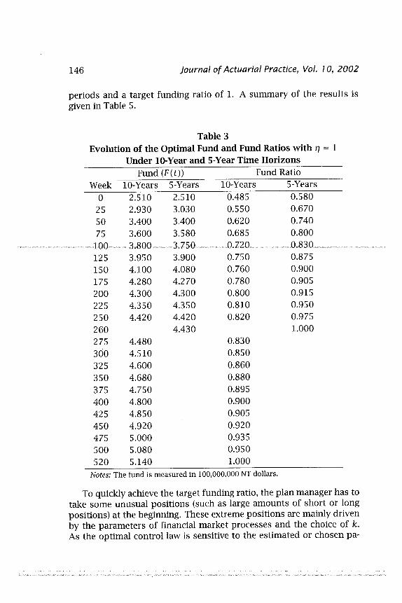
The optimal weekly contributions and contribution rates are shown in Table 2 for rJ = 1. The optimal weekly contributions and contribu­tion rates increase steadily with time. Such increases are reasonable because normal costs increase with the aging of the employees in the plan. Table 3 show the resulting fund when the pension plan adopts the optimal investment strategies under different evaluation periods (5 and 10 years) and a target funding ratio of 1. Table 4 shows the evolution of the optimal mix of stocks, bonds and cash under different evaluation

146 Journal of Actuarial Practice, Vol. 70, 2002

periods and a target funding ratio of 1. A summary of the results is given in Table 5.

Table 3 Evolution of the Optimal Fund and Fund Ratios with '1 = 1

Under lO-Year and 5-Year Time Horizons Fund (F(t)) Fund Ratio

Week 10-Years 5-Years 10-Years 5-Years 0 2.510 2.510 0.485 0.580

25 2.930 3.030 0.550 0.670 50 3.400 3.400 0.620 0.740 75 3.600 3.580 0.685 0.800

100 3.800 3.750 0.720 0.830 125 3.950 3.900 0.750 0.875 150 4.100 4.080 0.760 0.900 175 4.280 4.270 0.780 0.905 200 4.300 4.300 0.800 0.915 225 4.350 4.350 0.810 0.950 250 4.420 4.420 0.820 0.975 260 4.430 1.000 275 4.480 0.830 300 4.510 0.850 325 4.600 0.860 350 4.680 0.880 375 4.750 0.895 400 4.800 0.900 425 4.850 0.905 450 4.920 0.920 475 5.000 0.935 500 5.080 0.950 520 5.140 1.000

Notes: The fund is measured in 100,000,000 NT dollars.

To quickly achieve the target funding ratiO, the plan manager has to take some unusual positions (such as large amounts of short or long positions) at the beginning. These extreme positions are mainly driven by the parameters of financial market processes and the choice of k. As the optimal control law is sensitive to the estimated or chosen pa-

Chang: Dynamic Funding and Investment Strategy 147

rameters, the plan manager should pay close attention to the choice of parameters.

Table 4 Proportions of Stocks, Bonds, and Cash

Under lO-Year and 5-Year Time Horizons with 17 = 1 10-Year Horizon 5-Year Horizon

Weeks Stocks Bonds Cash Stocks Bonds Cash 0 -4.100 8.800 -3.700 -3.800 8.800 -4.000

25 -2.750 4.800 -1.050 -2.250 4.200 -0.950 50 -1.400 2.600 -0.200 -1.350 2.500 -0.150 75 -0.650 1.600 0.050 -0.750 1.900 -0.150

100 -0.250 1.000 0.250 -0.400 1.400 0.000 125 -0.200 0.500 0.700 -0.250 0.700 0.550 150 -0.050 0.300 0.750 -0.060 0.300 0.760 175 -0.010 0.150 0.860 -0.010 0.150 0.860 200 0.000 0.050 0.950 0.001 0.050 0.949 225 0.000 0.001 0.999 -0.001 0.002 0.999 250 0.010 0.002 0.988 0.010 0.005 0.985 260 0.012 0.200 0.788 275 0.015 0.004 0.981 300 0.010 0.006 0.984 325 0.000 0.002 0.998 350 0.005 0.003 0.992 375 0.020 -0.050 1.030 400 0.001 0.000 0.999 425 0.005 -0.100 1.095 450 0.080 -0.200 1.120 475 0.004 -0.100 1.096 500 0.001 0.005 0.994 520 -0.100 0.500 0.600

...... >I:>-00

Table 5 Statistics on Asset Weights

Period Asset Class Minimum Median Mean Maximum Standard Deviation Given 11 = 0.75 and k = 0.0001

5 Years stock -0.7057 -0.0421 -0.1203 0.0061 0.1672 10 Years stock -0.7108 -0.0034 -0.0625 0.1083 0.1636 5 Years long term bond -0.0728 0.1792 0.2853 1.5888 0.3434 '-c

10 Years long term bond -0.2357 -0.0154 0.1272 1.6067 0.3655 s:: "" ~

5 Years cash 0.1132 0.8697 0.8350 1.0668 0.1809 ~

10 Years cash 0.1031 1.0175 0.9354 1.1399 0.2076 c -., ):.

'" .-. Given 11 = 1.00 and k = 0.0001 s::

t:\

5 Years stock -3.9395 -0.1611 -0.6277 0.0024 0.9193 "" ~ 10 Years stock -4.0801 -0.0076 -0.3197 0.0950 0.7961 '1J

5 Years long term bond -0.0489 0.7039 1.4995 8.8692 1.8794 2i '" .-.

10 Years long term bond -0.2082 0.0147 0.7282 8.8981 1.6783 rio !I>

5 Years cash -3.9653 0.4364 0.1281 1.0465 0.9769 ~ 10 Years cash -3.9161 0.9929 0.5915 1.1188 0.8932

,5:J I\J a a I\J

Chang: Dynamic Funding and Investment Strategy 149

The funding ratio volatility and the trading activity volatility increase with the difference between the current funding ratio and the target funding ratio. Notice that the volatility of trading volatilities, fund lev­els, and funding ratios when 17 = 1 are greater than those 17 = 0.75. This is reasonable because the larger the difference is, the more the assets have to be increased and thus the more aggressive the trading must be. Furthermore, we observe that shorter evaluation periods result in higher volatilities. A possible explanation is that shorter evaluation pe­riods make the optimal trading strategies more sensitive to financial markets because the plan manager has a shorter time to achieve the goal.

5 Summary and Closing Comments

Stochastic control is potentially a helpful tool for managing pension plans. It represents a significant improvement over the one-period ap­proach traditionally used by plan managers because it can explicitly consider the inter-period dynamics and aim at long-term rather than short-term optimality. Furthermore, dynamic control models can si­multaneously handle plan funding policies and investment decisions.

Our model is the most comprehensive one so far as it combines the merits from different models. The Haberman and Sung (1994) ap­proach is used to develop our objective function, Le., we consider the contribution risk (the stability of contributions) and the solvency risk (the security of funds). The Brennan, Schwartz, and Lagnado (1997) model is used to enlarge the set of investable assets so that it contains both risk-free and risky assets. For liabilities, we employ the stochastic simulations in Chang (1999, 2002) that explicitly characterize the plan members. These allow us to derive a system of differential equations, for which the solution represents optimal funding poliCies and asset al­locations. We then apply the theoretical model to an actual Taiwanese pension plan and numerically obtain optimal solutions.

There are three areas for further research:

• One may add short sale constraints into our model because our optimal strategies usually involve certain amount of short sales. Most pension funds, however, are not allowed to engage in short sales because of the associated downside risk;

• One may want to include transaction costs. Note that high trans­action costs may reduce the relative advantage of active trading

150 Journal of Actuarial Practice, Vol. 10, 2002

to passive trading, which might result in different optimal trading strategies; and finally,

• Include optimal hedging policies.

References

Anderson, AW. Pension Mathematics for Actuaries, 2nd ed. Winsted, Conn.: Actex Publication, 1992.

Bellman, R. Dynamic Programming. Princeton, N.J.: Princeton Univer­sity Press, 1957.

Boyle, P. and Yang, H. "Asset Allocation with Time Variation in Expected Returns." Insurance: Mathematics and Economics 21 (1997): 201-218.

Brennan, M.J. and Schwartz, E.S. "An Equilibrium Model of Bond Pricing and a Test of Market Efficiency." Journal of Financial and Quantita­tive Analysis 17 (1982): 301-329.

Brennan, M.l. and Schwartz, E.S. "The Use of Treasury Bill Futures in Strategic Asset Allocation Programs." In Worldwide Asset And Li­ability Modeling. (J.M. Mulvey and W.T. Ziemba, Eds.) Cambridge, England: Cambridge University Press, (1998): 205-230.

Brennan, M.J., Schwartz, E.S., and Lagnado, R. "Strategic Asset Alloca­tion." Journal of Economics, Dynamics and Control 21 (1997): l377-1403.

Cairns, AJ.G. "Pension Funding in a Stochastic Environment: The Role of Objectives in Selecting An Asset-Allocation Strategy." Proceedings of the 5th AFIR International Colloquium 1 (1995): 429-453.

Cairns, AJ.G. "Continuous-Time Stochastic Pension Funding Modelling," Proceedings of the 6 th AFIR International Colloquium 1 (1996): 609-624.

Cairns, Al.G. "Some Notes on the Dynamics and Optimal Control of Stochastic Pension Fund Models in Continuous Time." ASTIN Bul­letin 30 (2000): 19-55.

Chang, S.c. "Optimal Pension Funding Through Dynamic Simulations: The Case of Taiwan Public Employees Retirement System." Insur­ance: Mathematics and Economics 24 (1999): 187-199.

Chang, S.c., "Realistic Pension Funding: A Stochastic Approach. "Journal of Actuarial Practice 8 (2000): 5-42.

Chang: Dynamic Funding and Investment Strategy 151

Chang, S.c. and Cheng, H.Y. "Pension Valuation Under Uncertainty: Im­plementation of a Stochastic and Dynamic MOnitoring System." Jour­nal of Risk and Insurance 69, no. 2 (2002): 171-192.

Fleming W.H. and Rishel, R.W. Deterministic and Stochastic Optimal Con­trol. New York, N.Y.: Springer-Verlag, 1975.

Haberman, S. and Sung, J.H. "Dynamic Approaches to Pension Funding." Insurance: Mathematics and Economics 15 (1994): 151-162.

Karatzas, I., Lehoczky, J.P., Sethi, S.P., and Shreve, S.E. "Explicit Solution of a General Consumption/Investment Problem." Mathematics of Operations Research 11 (1986): 262-292.

Merton, R.C. Continuous Time Finance. Oxford, England: Blackwell, 1990.

Merton, R.C. "Optimum Consumption and Portfolio Rules in a Continu­ous Time Model." Journal of Economic Theory 3 (1971): 373-413.

O'Brien, T. "A Stochastic-Dynamic Approach to Pension Funding." In­surance: Mathematics and Economics 5 (1986): 141-146.

O'Brien, T. "A Two-Parameter Family of Pension Contribution Func­tions and Stochastic Optimization." Insurance: Mathematics and Economics 6 (1987): 129-134.

Petit, M.L. Control Theory and Dynamic Games in Economic Policy Anal­ysis. Cambridge, England: Cambridge University Press, 1990.

Runggaldier, W.J "Concept and Methods for Discrete and Continuous Time Control Under Uncertainty." Insurance: Mathematics and Eco­nomics 22 (1998): 25-39.

Samuelson, P. "Lifetime Portfolio Selection by Dynamic Stochastic Pro­gramming." Review of Economics and Statistics (1969): 239-246.

Sharpe, W.F. "Capital Asset Prices with and without Negative Holdings." Journal of Finance 64, no. 2 (1991): 489-509.

Schal, M. "On Piecewise Deterministic Markov Control Processes: Con­trol of Jumps and of Risk Processes in Insurance." Insurance: Math­ematics and Economics 22 (1998): 75-91.

Sorensen, C. "Dynamic Asset Allocation and Fixed Income Management." Journal of Financial and Quantitative Analysis 34, no. 4, (1999): 513-531.

Winklevoss, H.E. Pension Mathematics with Numerical Illustrations, 2nd Edition. Philadelphia, Pa.: Pension Research Council, University of Pennsylvania, 1993.

152 Journal of Actuarial Practice, Vol. 10, 2002

Appendix

Table Al Simplified Male Service Table

Survival Probabilities

x piT) x piT)

15 0.860048 38 0.937401 16 0.859854 39 0.937279 17 0.859326 40 0.983539 18 0.859181 41 0.983369 19 0.859278 42 0.983176 20 0.801437 43 0.982957 21 0.801529 44 0.982763 22 0.801620 45 0.982559 23 0.801712 46 0.982352 24 0.801708 47 0.982149 25 0.881447 48 0.981952 26 0.881441 49 0.981673 27 0.881436 50 0.990293 28 0.881438 51 0.989965 29 0.881445 52 0.989596 30 0.937983 53 0.989173 31 0.937946 54 0.988972 32 0.937887 55 0.988738 33 0.937804 56 0.988465 34 0.937741 57 0.988150 35 0.937668 58 0.987794 36 0.937585 59 0.987288 37 0.937496 60 0

Note: piT) = Probability a male plan member age x remains in the plan at age x + 1.

Chang: Dynamic Funding and Investment Strategy 153

Table A2 Simplified Female Service Table

Survival Probabilities

x piT) x piT)

15 0.860180 38 0.938062 16 0.860134 39 0.938021 17 0.860081 40 0.984412 18 0.860059 41 0.984340 19 0.860054 42 0.984258 20 0.802068 43 0.984166 21 0.802065 44 0.984053 22 0.802064 45 0.983935 23 0.802063 46 0.983814 24 0.802061 47 0.983691 25 0.881830 48 0.98357l 26 0.881818 49 0.983423 27 0.881800 50 0.992203 28 0.881781 51 0.992035 29 0.881759 52 0.991851 30 0.938305 53 0.991652 31 0.938279 54 0.991392 32 0.938258 55 0.991124

Note: p1T) = Probability a female plan

member age x remains in the plan at age x + 1.

Table A3 Basic Statistics on New Entrants

Age Number of Average Interval New Entrants Annual Salary

15 19 82 23,356 20 24 163 27,660 25 29 273 38,404 3034 88 38,7l8 35 39 17 46,297 40 44 7 43,305 45 49 4 36,053

154 Journal of Actuarial Practice, Vol. 10, 2002