Dynamic Hello/Timeout timer adjustment in routing

protocols for reducing overhead in MANETs

Nelson HERNANDEZ-CONS, Shoji KASAHARA∗, Yutaka TAKAHASHI

Graduate School of Informatics, Kyoto University36-1, Yoshida-honmachi, Sakyo-ku, Kyoto 606-8501, Japan

Abstract

With the recent advancement and extensive spread of mobile devices, es-

tablishing a network with those devices has become more important than

ever before. MANETs (Mobile Ad-hoc NETworks) have become a promising

solution to set up a network with any mobile device. Routing in MANET

is still a difficult task since the mobility of the nodes affects the local con-

nections and makes the network topology change constantly. Traditional

routing protocols in MANET work sending periodic messages to realize the

changes in the topology in order to maintain the local connections up-to-

date. However, sending periodic messages at a fixed rate can cause overhead

in situations where it can be prevented and thus reduced. In this paper,

we introduce a scheme to improve the performance of the routing protocols

used in MANET focusing on the reduction of the overhead. In the pro-

posed scheme, instead of sending periodic messages at a fixed rate, we use

a link change rate estimation to dynamically adjust the rate at which each

node sends the control messages. The link change rate estimation is based

∗Corresponding author. Tel.:+81-75-753-5493; Fax:+81-75-753-3358.Email address: kasahara@ieee.org (Shoji KASAHARA)

Preprint submitted to Computer Communications June 24, 2009

on the constant measurement of the local connectivity that reflects the net-

work conditions. We evaluate the performance of our scheme using ns-2 and

we compare it to other approaches to show its advantages. With the usage

of our scheme, we notice a considerable reduction of the overhead without

sacrificing the overall performance of the tested protocols.

Key words: MANET, soft state, overhead, AODV, OLSR, ns-2

1. Introduction

MANETs (Mobile Ad-hoc NETworks) are wireless mobile networks that

are set up on the spot without prior preparation of any infrastructure, that is,

in an ad hoc fashion. The lack of infrastructure, routers, servers and cables

makes MANETs a fast, low-cost and convenient way to deploy a network

with the use of mobile devices such as cellular phones, smart phones or

small laptop computers. Moreover, MANETs can offer a rapid solution for a

network in situations such as military operations, disaster recovery, vehicle-

to-vehicle communication networks, conferences, events or shows, airport

terminals or for personal area networks connecting smart phones with other

wearable devices.

There are several routing protocols for MANET, although very few are

standardized. Routing in MANET is a difficult issue as several factors affect

the stability of the network and make the topology highly dynamic. The

routing protocols in MANET use several mechanisms to keep track of the

changes in the network, for example, link layer sensing of the wireless links,

or the usage of Hello messages at the routing level, which is referred to as

soft state signaling.

2

In soft state signaling, a node periodically broadcasts Hello messages to

keep track of valid links and also to advertise its presence in the network.

Traditional protocols use a fixed time interval to send these Hello messages,

which is not optimal. For example, if the nodes in a network do not move,

the links of the nodes will not change; so sending Hello messages at a fixed

rate will only cause unnecessary overhead in the network. On the other hand,

if the nodes are moving too fast, sending Hello messages at a fixed rate might

advertise the links too late; so when a node sends a packet to a neighbor,

that neighbor might not be in the same position anymore, in which case the

packet will simply be dropped. The node will then have to exchange more

messages to find a way to route the pending packets.

Overhead (control messages including Hello messages) is necessary to keep

the nodes updated with the changes in the network. However, minimizing the

overhead in MANETs is critical since the mobile nodes have a very limited

amount of energy. Reducing the overhead helps the nodes to reduce the

amount of energy used, so that they last longer in the network. Moreover,

when the overhead is low, congestions are less likely to occur.

In this paper, we propose an overhead-reducing scheme consisting of three

mechanisms to regulate the Hello timer and its timeout. First, we measure

the link change rate by monitoring the number of acquired and lost links.

If a node has a link change rate close to zero, its neighborhood remains

unchanged. Conversely, if a node has a high link change rate, it means its

neighborhood has changed. With this particular assumption, we can set the

Hello timer to an adequate value. In stable networks, the value of the Hello

timer can be higher so that there is no unnecessary overhead, and in highly

3

dynamic networks, the value should be small to keep track of the changes in

the network. With the value of the Hello timer set dynamically, we also set

the Timeout timer to an adequate value. When neighbors stay an adequate

amount of time in the routing tables, unnecessary route requests will not

be issued, thus further reducing the overhead. Finally, when Hello messages

are scheduled to be sent in the future and the network changes suddenly, we

reschedule the Hello message sooner in time in order to react to the sudden

changes.

We expect a considerable reduction of the overhead introduced in the

network. To verify the effectiveness of the proposed scheme, we evaluate its

performance using the network simulator ns-2.

The rest of this paper is organized as follows. In Section 2, we give

an overview of MANET and signaling mechanisms. We also present related

works on the issue of signaling and overhead in MANETs. Section 3 describes

the adaptive timer scheme. Numerical examples to evaluate the effectiveness

of the scheme are presented in Section 4. Finally, conclusions and future

work are presented in Section 5.

2. Related work

In this section we present a brief overview of MANET and soft state

signaling related approaches.

In soft state signaling, each node in the network sends a refresh message

periodically in the form of a broadcast to all the neighboring nodes. This

message is sent to refresh the state that reflects the conditions of the network.

The period that a node waits until a message is sent, is called the refresh

4

period. In soft state signaling, the state is automatically removed at the

receivers if no refresh message is received after some specific time called the

timeout period.

For the purposes of our study, we focus on the Hello timer on the sender

side and on the Neighbor Timeout timer on the receiver side. The Hello

timer value controls the period to wait until a Hello message needs to be

sent, while the Neighbor Timeout timer controls the period of time a link

towards a neighbor is considered valid. Traditional approaches use fixed

values for those two timers. For example, standard AODV (7) proposes a

Hello timer of one second and a timeout timer of two seconds.

Starting from the traditional approach of fixed timer values in the proto-

cols, there have been several adaptive timer approaches for routing protocols

in MANETs. Basagni et al. (1) proposed DREAM (Distance Routing Effect

Algorithm for Mobility) which considers the possible usage of mobility as a

way to control the refresh timer to broadcast messages. In DREAM, the au-

thors state that a node broadcasts a control message according to its speed.

The faster a node moves, the more often it broadcasts messages. Conversely,

the slower a node moves, the fewer the control messages it sends. In their

approach, the speed of the node, which can be obtained by mechanisms such

as GPS (Global Positioning System), is the sole parameter used to control

the rate to send messages. However, the individual speed of one node doesn’t

determine the mobility of the network. In fact, it is very difficult for a single

node to decide, using only its own speed, whether the network is changing

fast or the network remains stable. Moreover, the authors simulated some

scenarios with all the nodes having the same speed throughout the simula-

5

tions.

Camp et al. (2) proposed an approach that takes into account the trans-

mission range of the node as well as its speed to regulate the sending rate of

control messages. Moreover, there is a distinction between close nodes and

far-away nodes. Close nodes receive more periodic refresh messages while

far-away nodes do not receive those messages very often under the assump-

tion that far away nodes “appear” to move more slowly from the sender’s

point of view. This particular model uses several constant values to modify

the refresh timer.

Fast OLSR (10) by Benzaid et al. is an extension of standard OLSR that

works in two modes: fast moving mode and the default normal mode. In

normal mode, the protocol behaves like standard OLSR. In the fast moving

mode, the protocol uses a Hello timer with a fixed smaller value obtained

from simulation experiments. In (10), some scenarios are defined according

to the speed of the nodes and then the values of the timers are calculated

and fixed, which then makes the protocol extension not fully adaptive.

Huang et al. (4) give an algorithm based on the link change rate. A link

is a local connection with a neighbor, and the link change rate measures the

change in the set of links of a node through time. The link change rate is cal-

culated using a formula given by an analytical model developed by Samar and

Wicker (3). The used formula takes into account the speed of one node while

the other nodes’ speeds are assumed random. However, there are several pa-

rameters that have to be known for the formula to be used in real situations,

such as the density of the network, the maximum and minimum speeds of

the nodes and the direction of motion of the nodes. Some parameters can

6

be obtained through mechanisms such as GPS (Global Positioning System)

while others are more difficult to accurately estimate. Huang’s algorithm is

based on a Multiplicative Increase Additive Decrease (MIAD) controller to

adapt the refresh timer of a protocol. His approach provides an adaptive

solution to dynamically modify the refresh timer, but the dependency on

network measurements to compute the parameters used in the formula for

the link change rate makes it questionable for real implementations.

In (6), Sharma et al. proposed a scheme to control the timer at the sender

and also at the receiver. Their approach is adaptive to the volume of control

traffic and the available bandwidth on the link. The receiver has to estimate

the Timeout timer from the rate at which the sender sends data, which can

work in fixed wired networks but is not a reliable approach for MANET due

to the dynamics of the network. In fact, in their study they focus on fixed

wired networks and not wireless networks, so the methodology of their study

is not directly applicable to MANETs.

3. Proposed scheme

In this section, we present the details of the proposed scheme to reduce

the soft state overhead in MANET routing protocols. We base our study

on the constant measurement of the link change rate. In the following, we

consider a link as a wireless direct connection between two nodes that are

neighbors and are therefore within the transmission range of each other. We

also consider a stable network as a network with few topology changes, that

is, the connections remain stable among the nodes. In other words, there are

very few new links or lost links in the network. In general, a low mobility

7

network can be considered as a stable network.

The goal of the scheme is to dynamically adjust the Hello timer and the

Timeout timer according to the conditions of the network. For example, in

a high mobility network (with frequent topology changes) it is desirable to

use small values for the timers to quickly detect the changes in the network.

On the other hand, in a low mobility network where the topology remains

stable and with few changes, a large value for the timers is more effective to

reduce the overhead.

In order to decide whether the mobility of the network is high or low,

we use a simple way to approximate in real time the link change rate. The

link change rate expresses how the number of available links changes through

time and is expressed in [links/sec]. The changes occur when a new link is

established or an active link is lost.

In the following, we first explain the measurement of the link change rate

and then the three mechanisms in detail.

3.1. Computation of the Link Change Rate (LCR)

We assume each node has a neighbor table to store the addresses of its

neighbors. Consider node A and node B in a MANET, both have just moved

within the transmission range of each other so that they can become neigh-

bors. Node A receives a Hello message from node B, so node A considers

node B as a new neighbor and stores node B’s address in its neighbor table.

Therefore, node A has created a new link towards node B. We use a counter,

newLinkCounter, to keep track of the number of new links. Similarly, if node

A and node B are already neighbors, and node B departs from the MANET,

node A will erase node B’s entry from its neighbor table according to the

8

Timeout timer. When the entry for node B is erased, node A loses the link

towards node B. We use another counter, lostLinkCounter, to keep track

of the number of lost links. We then calculate the link change rate lcr with

the following expression:

lcr =newLinkCounter + lostLinkCounter

t, (1)

where t is the time elapsed since the last measurement. It is clear that this is

a very simple way to approach the link change rate. In previous approaches,

in order to determine whether a node is in a high mobility or low mobility

network, usually only its own speed is taken into account while the speed

of the rest of the nodes is ignored or assumed random. Consider node A in

a network and the set N as the set of node A’s neighbors. Let vA and VN

denote the speeds of node A and the average speed of the neighbors of A,

respectively. Notice that this approach includes both influences, vA and VN ,

since node A gains or loses links due to its own mobility, but also due to the

mobility of the rest of the nodes N .

Instead of using an instant value of the lcr, we calculate an average over

time using an EWMA (Exponential Weighted Moving Average) filter:

LCRest(k) = LCRest(k − 1)αEWMA + LCRsample(k)(1− αEWMA),

where LCRest(k) is the average over time, LCRest(k − 1) is the previous

estimated average, LCRsample(k) is the most recent measured value of the

link change rate calculated from (1) and αEWMA is the parameter of the

filter.

In most of the literature, the parameter αEWMA is normally adjusted to a

9

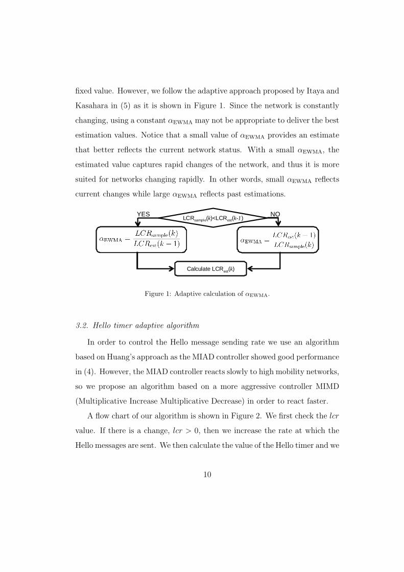
fixed value. However, we follow the adaptive approach proposed by Itaya and

Kasahara in (5) as it is shown in Figure 1. Since the network is constantly

changing, using a constant αEWMA may not be appropriate to deliver the best

estimation values. Notice that a small value of αEWMA provides an estimate

that better reflects the current network status. With a small αEWMA, the

estimated value captures rapid changes of the network, and thus it is more

suited for networks changing rapidly. In other words, small αEWMA reflects

current changes while large αEWMA reflects past estimations.

YES NOLCRsample(k)<LCRest(k-1)

Calculate LCRest(k)

Figure 1: Adaptive calculation of αEWMA.

3.2. Hello timer adaptive algorithm

In order to control the Hello message sending rate we use an algorithm

based on Huang’s approach as the MIAD controller showed good performance

in (4). However, the MIAD controller reacts slowly to high mobility networks,

so we propose an algorithm based on a more aggressive controller MIMD

(Multiplicative Increase Multiplicative Decrease) in order to react faster.

A flow chart of our algorithm is shown in Figure 2. We first check the lcr

value. If there is a change, lcr > 0, then we increase the rate at which the

Hello messages are sent. We then calculate the value of the Hello timer and we

10

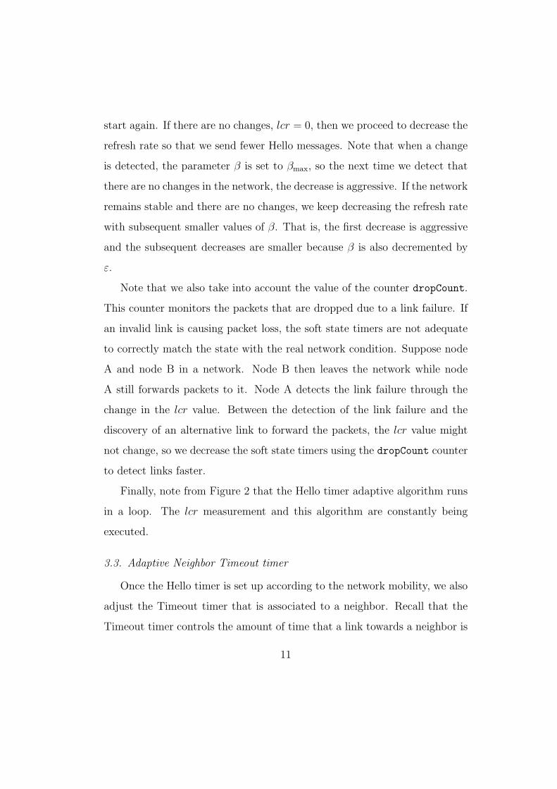
start again. If there are no changes, lcr = 0, then we proceed to decrease the

refresh rate so that we send fewer Hello messages. Note that when a change

is detected, the parameter β is set to βmax, so the next time we detect that

there are no changes in the network, the decrease is aggressive. If the network

remains stable and there are no changes, we keep decreasing the refresh rate

with subsequent smaller values of β. That is, the first decrease is aggressive

and the subsequent decreases are smaller because β is also decremented by

ε.

Note that we also take into account the value of the counter dropCount.

This counter monitors the packets that are dropped due to a link failure. If

an invalid link is causing packet loss, the soft state timers are not adequate

to correctly match the state with the real network condition. Suppose node

A and node B in a network. Node B then leaves the network while node

A still forwards packets to it. Node A detects the link failure through the

change in the lcr value. Between the detection of the link failure and the

discovery of an alternative link to forward the packets, the lcr value might

not change, so we decrease the soft state timers using the dropCount counter

to detect links faster.

Finally, note from Figure 2 that the Hello timer adaptive algorithm runs

in a loop. The lcr measurement and this algorithm are constantly being

executed.

3.3. Adaptive Neighbor Timeout timer

Once the Hello timer is set up according to the network mobility, we also

adjust the Timeout timer that is associated to a neighbor. Recall that the

Timeout timer controls the amount of time that a link towards a neighbor is

11

YES NO

LOOP @ t

LOOP @ h=1/r

Calculate lcrt

Is lcrt>0 or dropCount>0

Increase the refreshrate r = r x α

Initialize β = βmax

Decrease the refreshrate r = r x 1/β

Decrease ββ = β - ε

Hello timer h = 1/r

Broadcast Hello message

Figure 2: Algorithm to calculate the Hello timer based on the link change rate and the

packet drop count.

considered valid.

The aim of this mechanism is to reduce the overhead by preventing a

node from issuing a route request or search for a link. Again, consider node

A and node B within the transmission range of each other. Node B sends

Hello messages to node A, and node A stores node B in its neighbor table.

In a stable network, if the Timeout timer for node B is small, node A will

delete the entry for node B after a short period of time. If node B delays in

sending Hello messages, node A will have to send a route request or search

for a link which will lead to some exchange of messages from both sides.

If the Timeout timer for node B has a higher value, node A can continue

forwarding packets to node B without neither of them having to exchange

control messages. Thus, in stable networks it is desirable to have a higher

value of the Timeout to reduce overhead, while in highly dynamic networks

12

a shorter Timeout timer value is preferable.

AODV uses the following expression to calculate the Timeout timer for

each neighbor:

Neighbor expire = ALLOWED HELLO LOSS× HELLO INTERVAL,

where HELLO INTERVAL is the value of the Hello timer and its default

value is set to 1000 milliseconds. The other value ALLOWED HELLO LOSS

is a constant fixed to two. These values are fixed according to the RFC (7).

Instead of using the default value of HELLO INTERVAL, we use the dynamic

adaptive value of the Hello timer calculated with our adaptive algorithm.

For OLSR the neighbor timeout timer is also set, by default, to a constant

time:

Neighbor Hold Time = 3× REFRESH INTERVAL,

where REFRESH INTERVAL is set to two seconds. These values are also

fixed according to the RFC (9). Similar to AODV, we use the adaptive value

of the Hello timer instead of the fixed REFRESH INTERVAL value.

3.4. Reactive Hello message scheduling

The aim of this mechanism is to help the protocol to better react to

sudden changes in the network. Recall from previous sections that the lcr

value is constantly being monitored and therefore, Hello messages are being

scheduled to be sent in the future.

Suppose again a stable network where the Hello timer of node A has

reached a high value. Consequently, the next Hello message is scheduled far

in the future. If there is a sudden change in the network, it is desirable that

node A should not wait until the next Hello message to react. Instead, upon

13

noticing the sudden change in the network, we recalculate the Hello timer

and if the value of the new Hello timer is smaller than the previous one, we

reschedule the next Hello message sooner in time.

tHello msg

LCRt1

LCR computation

Hello msg

LCRt2

LCR computation

t1 t2

Figure 3: A Hello message scheduled at t1 is canceled and rescheduled at t2 as a result of

sudden changes in the links.

Consider a computation of the lcr at time t1. This yields a value for the

Hello timer ht1, and a Hello message is then scheduled at time t1 +ht1. Now,

suppose at time t2 there is a new computation of the lcr, and so a new value

for the Hello timer ht2 is also calculated. If t2 + ht2 < t1 + ht1, then the first

Hello message is canceled, and a new Hello message scheduled to be sent at

t2 + ht2.

4. Performance evaluation

In this section, we evaluate the overhead reduction of the proposed scheme

using the network simulator ns-2 (11) version 2.33. We simulate using two

protocols, the reactive protocol AODV (7) and the proactive protocol OLSR

(9). We use three different versions of these protocols: the original protocol, a

modified version implementing Huang’s DT MIAD approach (4) and finally,

a modified version of the protocol implementing our proposed scheme.

14

For our simulations, we first generate a set of different and random sce-

narios. We want to cover as many situations as possible so we have nodes

moving with random speeds uniformly distributed in the range [0,40] m/s.

In order to measure the link change rate as a function of the speed of the

nodes, we also introduce one node, namely node A, with deterministic speed

also in the range [0,40] m/s.

For each configuration of speed, we generate 100 different scenarios, and

we run the three versions of each protocol with each scenario. For one sce-

nario we run first the original protocol and we measure the link change rate,

the behavior of the Hello timer and some performance metrics discussed in

the next section. Then we run the exactly same scenario with the protocol

implementing Huang’s approach and finally with the proposed approach.

We use two different populations, n = 10 and n = 30 nodes to compare

the density of the network. Our simulations run for 100s using CBR (Con-

stant Bit Rate) sources sending packets of 512 bytes each, at a fixed rate of

2 packets per second. We show the detailed configuration of ns-2 in Table 1.

4.1. Performance metrics

In order to measure and compare the schemes, we use three performance

metrics: overhead, the CBR drop rate and the end-to-end (E2E) delay.

For the overhead, we are interested in the number of packets that were

received in the network, as these packets can cause collisions or congestion

in the network.

The CBR drop rate represents the efficiency of the protocol to deliver

the data from the source to the destination. We count the number of CBR

dropped packets #CBRdrop and the number of CBR sent packets #CBRsent.

15

Table 1: Basic simulation parameters.

Parameter Value

Antenna type Omni directional

Radio propagation Two-ray ground

Mobility model Random waypoint

MAC protocol IEEE 802.11

Pause time 1 [s]

Transmission range 250 [m]

Simulation area 500× 500 [m2]

Packet size 512 [byte]

Traffic model CBR @ 8 [Kb/s]

Simulation time 100 [s]

Routing protocols AODV, OLSR

We calculate the CBRdroprate with the expression

CBRdroprate =#CBRdrop

#CBRsent

.

The third measure is the end-to-end (E2E) delay. For the CBR packets,

we measure the time one packet takes to reach its final destination. We use

the following expression to calculate the E2E delay:

E2Edelay = trecv(pktID)− tsent(pktID),

where pktID is a number that uniquely identifies a packet, and trecv and tsent

are the times where the packet was received and sent, respectively.

16

3500

4000

4500

5000

5500

6000

6500

0 5 10 15 20 25 30 35 40Num

ber

of r

ecei

ved

cont

rol p

acke

ts [p

kt]

Speed [m/s]

Overhead (recv packets) with n=10 (AODV)

AODVAODV proposed

AODV Huang

42000

44000

46000

48000

50000

52000

54000

56000

0 5 10 15 20 25 30 35 40Num

ber

of r

ecei

ved

cont

rol p

acke

ts [p

kt]

Speed [m/s]

Overhead (recv packets) with n=30 (AODV)

AODVAODV proposed

AODV Huang

(a) Low density n = 10. (b) High density n = 30.

Figure 4: AODV comparison of the received overhead by the network.

It is desirable to maintain small amounts of overhead to reduce energy

consumption or congestions in the network. It is equally important to main-

tain a small value for the CBR drop rate, the better a protocol performs the

closer this metric will be to zero.

4.2. AODV results

We present in this subsection the results for AODV.

First, from Figure 4 we observe a decrease in the amount of overhead

that causes traffic in the network. The biggest decrease is achieved by the

approach proposed in this paper. This is due to the fact that our approach

reacts to the changes in the network, and when the network is stable (for

example at low speeds) fewer Hello messages are sent. Conversely, when the

network is not stable, our approach sends more Hello messages to adapt to

the changes in the network. There is a concrete reduction of the overhead of

almost 30% compared to the original AODV and almost 15% compared to

Huang’s. The three approaches follow a similar tendency due to the fact that

17

0

0.02

0.04

0.06

0.08

0.1

0 5 10 15 20 25 30 35 40

CB

R p

acke

t dro

p ra

te

Speed [m/s]

CBR packet drop rate with n=10 (AODV)

AODVAODV proposed

AODV Huang

0

0.02

0.04

0.06

0.08

0.1

0 5 10 15 20 25 30 35 40

CB

R p

acke

t dro

p ra

te

Speed [m/s]

CBR packet drop rate with n=30 (AODV)

AODVAODV proposed

AODV Huang

(a) Low density n = 10. (b) High density n = 30.

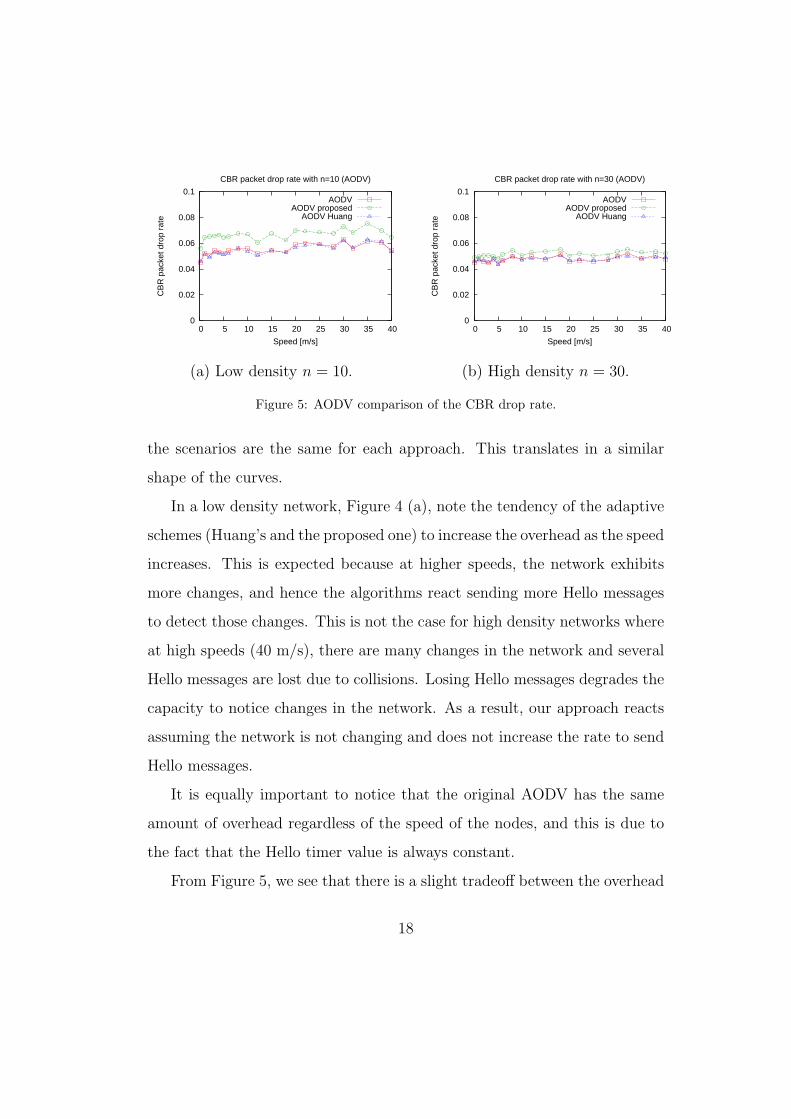
Figure 5: AODV comparison of the CBR drop rate.

the scenarios are the same for each approach. This translates in a similar

shape of the curves.

In a low density network, Figure 4 (a), note the tendency of the adaptive

schemes (Huang’s and the proposed one) to increase the overhead as the speed

increases. This is expected because at higher speeds, the network exhibits

more changes, and hence the algorithms react sending more Hello messages

to detect those changes. This is not the case for high density networks where

at high speeds (40 m/s), there are many changes in the network and several

Hello messages are lost due to collisions. Losing Hello messages degrades the

capacity to notice changes in the network. As a result, our approach reacts

assuming the network is not changing and does not increase the rate to send

Hello messages.

It is equally important to notice that the original AODV has the same

amount of overhead regardless of the speed of the nodes, and this is due to

the fact that the Hello timer value is always constant.

From Figure 5, we see that there is a slight tradeoff between the overhead

18

0

5

10

15

20

0 5 10 15 20 25 30 35 40

End

-to-

end

dela

y [m

s]

Speed [m/s]

End-to-end delay with n=10 (AODV)

AODVAODV proposed

AODV Huang

0

5

10

15

20

0 5 10 15 20 25 30 35 40

End

-to-

end

dela

y [m

s]

Speed [m/s]

End-to-end delay with n=30 (AODV)

AODVAODV proposed

AODV Huang

(a) Low density n = 10. (b) High density n = 30.

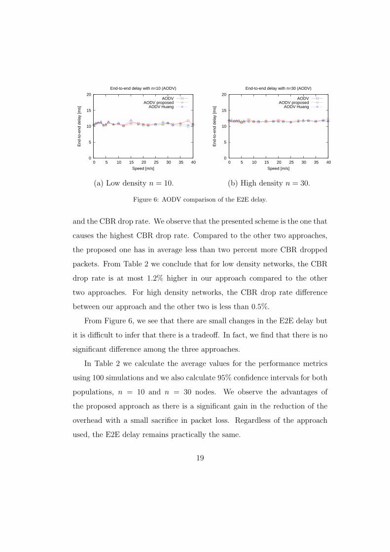
Figure 6: AODV comparison of the E2E delay.

and the CBR drop rate. We observe that the presented scheme is the one that

causes the highest CBR drop rate. Compared to the other two approaches,

the proposed one has in average less than two percent more CBR dropped

packets. From Table 2 we conclude that for low density networks, the CBR

drop rate is at most 1.2% higher in our approach compared to the other

two approaches. For high density networks, the CBR drop rate difference

between our approach and the other two is less than 0.5%.

From Figure 6, we see that there are small changes in the E2E delay but

it is difficult to infer that there is a tradeoff. In fact, we find that there is no

significant difference among the three approaches.

In Table 2 we calculate the average values for the performance metrics

using 100 simulations and we also calculate 95% confidence intervals for both

populations, n = 10 and n = 30 nodes. We observe the advantages of

the proposed approach as there is a significant gain in the reduction of the

overhead with a small sacrifice in packet loss. Regardless of the approach

used, the E2E delay remains practically the same.

19

Table 2: AODV performance metrics averages.Standard Huang Proposed

Overhead [pkt]

n=10 5494.77 4729.41 4005.05

95% 156.86 131.58 112.85

n=30 52324.08 47873.36 44425.77

95% 806.60 717.73 6573.19

CBR drop rate

n=10 0.0554 0.0546 0.0666

95% 0.0062 0.0062 0.0069

n=30 0.0476 0.0475 0.0517

95% 0.0035 0.0035 0.0037

E2E delay [ms]

n=10 10.82 10.79 10.52

95% 0.79 0.73 0.63

n=30 11.58 11.60 11.63

95% 0.44 0.47 0.49

4.3. OLSR results

Now we calculate the performance metrics for OLSR. We observe first

from Figure 7 that the proposed scheme considerably reduces the amount of

overhead that causes traffic in the network. The proposed approach reacts

adequately reducing the Hello message sending rate when the network does

not change frequently (at low speeds), and reacts increasing the rate when

there are more changes (at high speeds). Using our approach, there is a

concrete reduction of almost 33% compared to the original OLSR and almost

11% compared to Huang’s. Note that, for high density networks, higher

speeds do not necessarily increase the overhead as there are more collisions

in the network. Our approach is, in fact, more sensitive to the packet loss

considering that failing to receive Hello messages causes the approach to

continue increasing the Hello timer value more aggressively than Huang’s

approach. As a result, incorrect links lead to higher levels of packet loss.

20

2000

2500

3000

3500

0 5 10 15 20 25 30 35 40Num

ber

of r

ecei

ved

cont

rol p

acke

ts [p

kt]

Speed [m/s]

Overhead (recv packets) with n=10 (OLSR)

OLSROLSR proposed

OLSR Huang

18000

20000

22000

24000

26000

28000

30000

32000

34000

0 5 10 15 20 25 30 35 40Num

ber

of r

ecei

ved

cont

rol p

acke

ts [p

kt]

Speed [m/s]

Overhead (recv packets) with n=30 (OLSR)

OLSROLSR proposed

OLSR Huang

(a) Low density n = 10. (b) High density n = 30.

Figure 7: OLSR comparison of the received overhead by the network.

We observe from Figure 8 that there is still a slight tradeoff between

the overhead and the CBR drop rate. For low density networks, Fig. 8

(a), Huang’s approach and the proposed approach have similar CBR drop

rates. However, in high density networks, Fig. 8 (b), the proposed approach

exhibits the highest CBR drop rate. In populated networks, the probability

to have a collision is higher since there are many more nodes sending packets.

This fact raises the CBR drop rate of our approach compared to the other

two approaches.

Nevertheless, the differences are very small among the three approaches.

In the case of low density networks, the differences are smaller than one

percent, and for high density networks the differences are less than 0.5%.

Similar to the case for AODV, there is a tradeoff between the CBR drop

rate and the overhead reduction. However, using our approach the gain in

overhead reduction is more significant than the CBR packet loss rate.

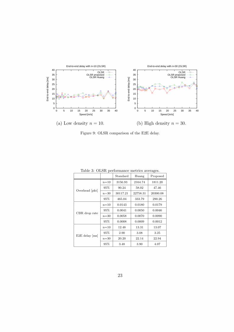
Figure 9 shows that, similar to AODV, the E2E delay in OLSR is not

greatly affected by the choice of the scheme. In low density networks, the

21

0

0.005

0.01

0.015

0.02

0.025

0.03

0 5 10 15 20 25 30 35 40

CB

R p

acke

t dro

p ra

te

Speed [m/s]

CBR packet drop rate with n=10 (OLSR)

OLSROLSR proposed

OLSR Huang

0

0.005

0.01

0.015

0.02

0.025

0.03

0 5 10 15 20 25 30 35 40

CB

R p

acke

t dro

p ra

te

Speed [m/s]

CBR packet drop rate with n=30 (OLSR)

OLSROLSR proposed

OLSR Huang

(a) Low density n = 10. (b) High density n = 30.

Figure 8: OLSR comparison of the CBR drop rate.

values are similar. However, for high density networks, packet loss causes a

larger E2E delay since, contrarily to AODV, an invalid link in OLSR causes

more delay due to the recalculation of routing tables. The E2E delay with our

approach is in average three milliseconds higher than the original approach

and one millisecond higher than Huang’s approach.

Finally, similar to AODV, the 100 simulations for OLSR are averaged and

95% confidence intervals are calculated. The summary is presented in Table

3.

22

0

5

10

15

20

25

30

35

40

0 5 10 15 20 25 30 35 40

End

-to-

end

dela

y [m

s]

Speed [m/s]

End-to-end delay with n=10 (OLSR)

OLSROLSR proposed

OLSR Huang

0

5

10

15

20

25

30

35

40

0 5 10 15 20 25 30 35 40

End

-to-

end

dela

y [m

s]

Speed [m/s]

End-to-end delay with n=30 (OLSR)

OLSROLSR proposed

OLSR Huang

(a) Low density n = 10. (b) High density n = 30.

Figure 9: OLSR comparison of the E2E delay.

Table 3: OLSR performance metrics averages.Standard Huang Proposed

Overhead [pkt]

n=10 3156.93 2164.74 1811.20

95% 90.24 58.02 47.46

n=30 30117.21 22758.31 20300.08

95% 465.04 333.79 290.26

CBR drop rate

n=10 0.0143 0.0180 0.0179

95% 0.0041 0.0050 0.0046

n=30 0.0058 0.0070 0.0090

95% 0.0008 0.0009 0.0012

E2E delay [ms]

n=10 12.48 13.31 13.07

95% 2.90 3.08 3.25

n=30 20.20 22.14 22.94

95% 3.48 3.90 4.07

23

5. Conclusions

In this paper, we considered the problem of the overhead in MANETs.

In order to tackle this issue, we proposed a scheme that can help to solve the

problem, and validated the effectiveness of the scheme by simulations. The

proposed mechanisms can be added as independent modules to the existing

protocols, or can be implemented inside the protocols but without changing

their architecture or the messages they exchange.

Through simulation experiments using different scenarios, we were able

to measure different metrics and compare the overall performance of the

proposed approach with the original protocols AODV and OLSR, and an-

other scheme to reduce the overhead proposed by Huang. With the proposed

scheme, the reduction of the overhead is greatly achieved with the minimal

cost of slightly increasing the drop rate in data traffic. Therefore, the pro-

posed approach outperforms normal standard AODV and OLSR protocols

as well as the other approach. The simplicity of our scheme and the inde-

pendence of any other tools (like GPS) make it suitable for implementations

and applications in real scenarios.

For further work, we plan to analyze the dependency between the link

change rate and the protocols. We also plan to develop an approach that

does not require configuring any parameters.

References

[1] S. Basagni, I. Chlamtac, V. R. Syrotiuk and B. A. Woodward, “A Dis-

tance Routing Effect Algorithm for Mobility (DREAM),” in Proceedings

of the 4th annual ACM/IEEE International Conference on Mobile Com-

24

puting and Networking (MOBICOM) ’98, Dallas, USA, October 1998,

pp. 76-84.

[2] T. Camp, J. Boleng and L. Wilcox, “Location Information Services in

Mobile Ad Hoc Networks,” in Proceedings of the IEEE International

Conference on Communications (ICC), 2002, pp. 3318-3324.

[3] P. Samar and S. B. Wicker, “On the Behavior of Communication Links

of a Node in a Multi-hop Mobile Environment,” in Proceedings of the

5th ACM International Symposium on Mobile Ad hoc Networking and

Computing (MobiHoc), Tokyo, Japan, 2004, pp. 145-156.

[4] Y. Huang, S. Bhatti and S. Sorensen, “Adaptive MANET Routing for

Low Overhead,” in International Symposium on a World of Wireless,

Mobile and Multimedia Networks (WoWMoM 2007), June 2007, pp. 1-6.

[5] N. Itaya and S. Kasahara, “Dynamic parameter adjustment for

available-bandwidth estimation of TCP in wired-wireless networks,”,

Elsevier Computer Communications, June 2004, vol. 27 issue 10, pp.

976-988.

[6] P. Sharma, D. Estrin, S. Floyd and V. Jacobson, “Scalable Timers for

Soft State Protocols,” in Proceedings of the Sixteenth Annual Joint Con-

ference of the IEEE Computer and Communications Societies (INFO-

COM ’97), Kobe, Japan, April 1997, p. 222-229.

[7] C. E. Perkins, E. M. Belding-Royer, and R. Das Samir; Ad hoc On-

Demand Distance Vector (AODV) Routing, IETF RFC 3651, July 2003;

http://www.ietf.org/rfc/rfc3561.txt.

25

[8] I. D. Chakeres and E. M. Belding-Royer, “The utility of Hello Messages

for determining Link Connectivity,” in Proceedings of the 5th Interna-

tional Symposium on Wireless Personal Multimedia Communications

(WPMC), Honolulu, October 2002, vol. 2, pp. 504-508.

[9] T. Clausen and P. Jaquet; Optimized Link State Rout-

ing Protocol (OLSR), IETF RFC 3626, October 2003;

http://www.ietf.org/rfc/rfc3626.txt.

[10] M. Benzaid, P. Minet and K. Agha, “Integrating Fast Mobility in the

OLSR Routing Protocol,” in Proceedings of the Fourth IEEE Conference

in Mobile and Wireless Communications Networks, Stockholm, Sweden,

September 2002, pp. 217-221.

[11] The Network Simulator: ns-2, http://www.isi.edu/nsnam/ns/.

26