Dynamic Landmark Triangles: A Simple and EfficientMechanism for Inter-Host Latency Estimation ∗

Zhihua WenElectrical Engineering & Computer Science

Case Western Reserve Universityzhihua.wen@case.edu

Michael RabinovichElectrical Engineering & Computer Science

Case Western Reserve Universitymisha@eecs.case.edu

ABSTRACTThis paper describes a simple and efficient approach to es-timate the network latency between arbitrary Internet hosts.We use three landmark hosts forming a triangle in two-dimensionalspace to estimate the distance between arbitrary hosts withsimple trigonometrical calculations. To improve the accu-racy of estimation, we dynamically choose the "best" tri-angle for a given pair of hosts using a heuristic algorithm.Experiments using several data sets of measured host-pairlatencies, as well as a live Internet study, demonstrate theaccuracy and efficiency of our approach.

1. INTRODUCTIONThe modern Internet is experiencing a rapid growth

in large-scale distributed applications utilizing overlayand peer-to-peer networks. The performance and scal-ing properties of these applications crucially dependon exercising communication paths according to net-work distances between hosts. Furthermore, the highscale of these systems often stipulates hierarchical de-sign, which typically relies on host clustering based onnetwork proximity. For example, content delivery net-works, such as Akamai and ICDS by AT&T, use dis-tance estimation to direct clients to the closest edgeservers for content download. In peer-to-peer file shar-ing applications like BitTorrent or Gnutella, each peercan benefit by selecting the closest peers to itself. Net-work clustering is fundamental to hierarchical P2P sys-tems, such as Gnutella 2, where super peers representclusters of neighboring hosts, and to large-scale Internetcharacterizations and monitoring [2, 12, 13]. Unfortu-nately, the scale of these systems often makes directon-demand distance measurements between hosts im-practical.A number of approaches have been proposed to han-

dle this problem by predicting the distance rather thanmeasuring it directly. Different approaches are tailoredfor different applications. In particular, IDMaps [7]aims at mapping inter-host distances on the global In-

∗This work is supported by the National Science Foundationunder Grant No. 0721890. The approach of the presentpaper was initially outlined in a position paper [33].

ternet scale. King [9] has a unique ability to estimatedistance between uncooperative hosts, even if they donot respond to probes. Coordinate-based techniques[26, 25, 28, 19, 31, 3, 4] map hosts to points in a met-ric space. These techniques are especially well-suitedin applications that reuse host coordinates for multipletasks since these tasks can be accomplished without fur-ther costs. Meridian [35] addresses the problems relatedto server selection, approaching them not through pre-diction but through actual measurements between thetarget host and exponentially narrowing set of servercandidates.In this paper, we propose an approach that targets

applications that do not require full network position-ing of hosts but only inter-host distances. This includesa wide range of applications such as overlay topologyformation, server selection, and node clustering men-tioned earlier. Our approach is extremely simple but,as we show through extensive experiments, is accurateand efficient at this task. Unlike full network position-ing techniques, we employ only three landmarks, form-ing a triangle in a two-dimensional Euclidean space, toestimate the distance between a pair of end hosts usingsimple trigonometrical calculations. However, we use arelatively large number of potential landmarks and care-fully select only three of them for any given prediction.Having a large number of potential landmarks allowsus to select the landmarks for each prediction that pro-duce high accuracy estimates. Using a small numberof landmarks for actual probing and computations keepthe overheads low. Thus, our approach represents atradeoff of achieving high accuracy and low overheadat the expense of having to deploy a relatively largenumber of well-dispersed potential landmarks.Our estimation involves two rounds of probes. In

the first round, we use a general, big triangle to ob-tain a rough distance estimates between each end hostand the landmark candidates. We then use these roughestimates as the basis for selecting another landmarktriangle, which is likely to obtain a high accuracy dis-tance estimation for the current end hosts. This secondtriangle produces the final distance estimation in the

1

second round of probing.We used a three-pronged approach to evaluate our

method and compare it with existing techniques. First,we evaluate it from the general prediction accuracy per-spective. Second, we study its performance in the con-text of some specific overlay applications - host cluster-ing and server selection. Third, we performed a a liveInternet study comparing the quality of server selectionin the Akamai content delivery network [1] using ourapproach and GNP, which was previously proposed fora similar task [30].Our results indicate that our simple technique is ac-

curate and efficient at the tasks it targets. For instance,in the live Akamai study, our approach showed a bet-ter selection quality than GNP with 1/7-th less probingtraffic. Thus, while different approaches are best-suitedfor different applications, we believe our method will bea valuable addition to the arsenal of overlay applicationdesigners.

2. RELATED WORKA number of approaches to inter-host distance esti-

mation have been proposed, with different approachesbetter suited for different applications. The King util-ity [9] estimates the distance between two arbitraryhosts by the distance between their authoritative DNSservers. It is more accurate for well-connected hoststhan residential hosts, which typically have high latencyto their DNS servers [34]. The IDMaps [7] platformutilized a large number of tracer hosts at strategic loca-tions in the Internet and estimated the distance betweentwo end hosts as the sum of the distance between eachhost and its nearest tracer plus the distance between thetwo tracers. IDMaps’s goal was to map rough inter-hostdistances on the global Internet scale within a factor oftwo of the real distances. The approach by Hotz [10] ex-ploits the observation that if triangle inequalities heldon the Internet, then the distance between two end-hosts would be bounded between the difference of thedistances from the end-hosts to a common landmarkand the sum of these distances. We discuss the IDMapsand Hotz’s approaches further in Section 5.3.Starting with the pioneering Global Network Posi-

tioning (GNP) approach [26], a number of current tech-niques are based on embedding hosts into a multidimen-sional metric space. Their key advantage is that oncea host’s coordinates are computed, they can be reusedfor distance estimation to any other mapped hosts withno additional overhead. GNP assigns coordinates to anode based on the measured distance from this nodeto a fixed set of well known hosts called landmarks.GNP is considerably more accurate than IDMaps andKing. However, owing to its use of simplex downhill tosolve a multidimensional nonlinear minimization prob-lem for error minimization, GNP incurs high compu-

tational overhead unless an application can effectivelyamortize it. Subsequent approaches [3, 25, 28] havedealt with a number of important issues such as secu-rity and landmark load but used the same underlyingestimation principle.Some approaches, including Virtual Landmarks [31]

and the Internet Coordinate System [19], utilize Lip-schitz embedding of hosts into a Euclidean space andreplace simplex downhill with an efficient linear approx-imation based on the principal component analysis. Inparticular, the Virtual Landmarks study [31] reportedsimilar accuracy to GNP, although on our data sets,this approach achieved its speedup at the expense ofaccuracy loss.Vivaldi [4] is a coordinates-based approach that re-

quires no fixed landmarks. Instead, each node con-stantly adjusts its own coordinates by communicatingwith other peers and following a mass-spring relaxationmodel whose minimum energy state determines the nodecoordinates. Vivaldi incurs no probing cost in its tar-geted peer-to-peer applications since it derives its mea-surements from regular P2P communication. We in-clude Vivaldi in our performance study. Big Bang Simu-lation (BBS) [29] is a somewhat similar approach whichmodels the network as a set of particles under the effectof the potential force field to determine node positions.Recently, the suitability of Euclidean embedding for

distance prediction has been questioned. In particular,Lua et al. [20] showed that these schemes appear tohave poor accuracy under a new relative rank loss met-ric, which the authors introduced as more meaningfulto a number of applications. Lee et al. [16] attributedthis issue to a large incidence of violations of triangleinequality on the Internet. We include relative rank lossas one of the general evaluation criteria of our approach.Unlike coordinate-based approaches, Meridian [35] does

not employ distance estimates but targets the server se-lection applications through direct measurements. Eachnode in Meridian organizes other nodes into rings ofdifferent radius, with a fixed number k of nodes ineach ring. To find the closest node to a given tar-get host, Meridian starts from a random node, andexplores a small set of nodes that are in the currentnode’s rings and at about the same distance from thecurrent node as the target. The query is then for-warded to the closest node to the target, and the searchterminates when the current node is the closest. Ac-cording to the Meridian study [35], its server selectionis an order of magnitude more accurate than that ofcoordinate schemes such GNP or Vivaldi. However,the query process takes O(logN) sequential forward-ing steps and O(klogN) probes, where N is the totalnumber of servers. According to [35], a system with2000 servers and k = 16 required just over 10K probingtraffic per query on average, or over a hundred probes.

2

Two recent studies report on the experiences withutilizing network distance estimations in real applica-tions. Ledlie et al [14] analyze the implementation ofthe Vivaldi algorithm in Azureus, a popular Bit-Torrentclient, and Szymaniak et al [30] report on utilizing GNPin the Google content delivery network. We return tothe latter paper in Section 7.2.Most distance estimation systems collect their mea-

surements by repeated probes between each pair of hostsand use the median or minimum value[26, 4] as the truenetwork distance. Ledlie et al. [15] introduce techniquesto reduce the necessary probing traffic between pairs ofhosts. Our approach can also benefit from their tech-niques.

3. LANDMARK TRIANGLESOur method estimates the distance between a pair

of hosts using their distance to three landmark hosts,and improves the accuracy of this estimate by selectingthe most appropriate landmarks for the given hosts. Asall distance prediction techniques, our method uses around-trip latency as the distance metric, which couldbe obtained using direct probes, such as ping or tcp-ping, or through passive measurements. Depending onthe application, the distances could be measured froma host to landmark or in the other direction. We con-sider these and other architectural details (e.g., who andwhen computes the distance estimates) when we discussspecific applications but simply assume the availabilityof RTT measurements in the general algorithm.

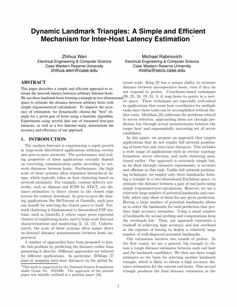
3.1 Basic AlgorithmOur basic idea is illustrated in Figures 1 and 2. Con-

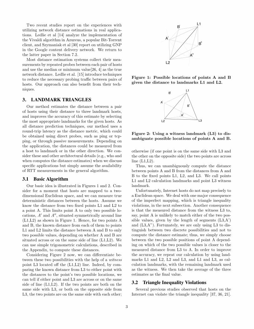
sider for a moment that hosts are mapped to a two-dimensional Euclidean space, and we can measure truedeterministic distances between the hosts. Assume weknow the distance from two fixed points L1 and L2 toa point A. This limits point A to only two possible lo-cations, A′ and A′′, situated symmetrically around line(L1,L2) as shown in Figure 1. Hence, for two points Aand B, the known distance from each of them to pointsL1 and L2 limits the distance between A and B to onlytwo possible values, depending on whether A and B aresituated across or on the same side of line (L1,L2). Wecan use simple trigonometric calculations, described inthe Appendix, to compute these distances.Considering Figure 2 now, we can differentiate be-

tween these two possibilities with the help of a witnesspoint L3 located off the (L1,L2) line. Indeed, by com-paring the known distance from L3 to either point withthe distances to the point’s two possible locations, wecan tell if either point and L3 are across or on the sameside of line (L1,L2). If the two points are both on thesame side with L3, or both on the opposite side fromL3, the two points are on the same side with each other;

L1

L2

A

BA

B

Figure 1: Possible locations of points A and Bgiven the distance to landmarks L1 and L2.

L2

A

B

B

A

L1

L3

Figure 2: Using a witness landmark (L3) to dis-ambiguate possible locations of points A and B.

otherwise (if one point is on the same side with L3 andthe other on the opposite side) the two points are acrossline (L1,L2).Thus, we can unambiguously compute the distance

between points A and B from the distances from A andB to the fixed points L1, L2, and L3. We call pointsL1 and L2 calculation landmarks and point L3 witnesslandmark.Unfortunately, Internet hosts do not map precisely to

a Euclidean space. We deal with one major consequenceof the imperfect mapping, which is triangle inequalityviolations, in the next subsection. Another consequenceis that the measured distance from the witness L3 to,say, point A is unlikely to match either of the two pos-sible values, given by the length of segments (L3,A’)and (L3,A”). Fortunately, we are only using L3 to dis-tinguish between two discrete possibilities and not tocompute the distance estimate; thus, we simply choosebetween the two possible positions of point A depend-ing on which of the two possible values is closer to themeasured distance from L3 to A. In order to improvethe accuracy, we repeat our calculation by using land-marks L1 and L2, L2 and L3, and L1 and L3, as cal-culation landmarks, with the remaining landmark usedas the witness. We then take the average of the threeestimates as the final value.

3.2 Triangle Inequality ViolationsSeveral previous studies observed that hosts on the

Internet can violate the triangle inequality [37, 36, 21].

3

These violations may lead to a situation when the mea-sured distances between hosts and landmarks allow nopossible mapping of hosts into the Euclidean plane.Recall that a given landmark triangle generates three

combinations of calculation and witness landmarks, andwe normally use the average of the three correspondingdistance results as the final distance estimate. Whensome pairs of the calculation landmarks yield no con-sistent host mappings, we simply consider only the re-maining pairs that do produce such mappings. In theextreme case, when all three pairs of calculation land-marks exhibit triangle inequality violation with one ofthe end hosts, we use the minimum of the three mea-sured indirect paths between the end hosts through eachof the three landmarks as the estimated distance. Thedegree of the triangle inequality violations and its effecton distance estimation accuracy is analyzed in Section5.It might appear that a more natural way to handle

the above case is to pick another landmark triangle, inthe hope it would not violate the triangle inequality.However, this would cost another round of network la-tency measurements between the new landmarks andeach end-host, which would be detrimental in a realtime distance estimation system that our approach tar-gets.

4. DYNAMIC TRIANGLE SELECTIONIt might appear natural to improve the triangles-

based approach by increasing the number of landmarksand using random selection of possible triangles to ob-tain a number of estimates, which could then be pro-cessed with standard statistical methods. However, wefound that this actually had a detrimental effect on ac-curacy. The reason is that the prediction error in differ-ent triangles is not random: some triangles are “good”,i.e., they produce highly accurate predictions and someare “bad”. Adding more random triangles does not nec-essarily improve the quality of the mix. It turns out thatone can characterize triangles in terms of the likely ac-curacy of their predictions. The next section examinesthese heuristics and uses them to develop an algorithmfor dynamic triangle selection.Our general approach to improve accuracy of distance

estimation is to have a large set of landmarks that couldpotentially be used in a landmark triangle and to selecta specific triangle for a particular pair of hosts. Ourgoal then is to develop a heuristic to dynamically selecta landmark that is likely to produce a high-accuracyestimate.

4.1 IntuitionWe develop our heuristic for dynamic triangle selec-

tion based on the following intuition. Consider Fig-ures 3(a), 3(b), and 3(c), where L1, L2 and L3 form a

big triangle, L1′, L2′ and L3′ form a small triangle, andwe want to estimate the distance between point A andB. On Figure 3(a), the points A and B are far apartand both are far away from the small triangle. Then,from the position of points A and B, the three land-marks L1′, L2′ and L3′ approximate one single point.Thus, the accuracy of this small triangle is very poor.For the big triangle of L1,L2 and L3, the distances be-tween the landmarks themselves and between points Aand B are comparable, so using big triangle in such acase can generate a relatively good estimate.Turning to Figure 3(b), both points A and B are

close to the small triangle and hence close to each other.From the view point of landmarks L1,L2 and L3, pointA and point B look like a single point, so the accuracyusing the big triangle is relatively poor in this case. Butfor the small triangle of landmarks L1′, L2′ and L3′, theinter-landmark distances are comparable to the distancebetween points A and B. Thus, using the small trianglein this case can generate a better estimate.Finally, on Figure 3(c), the points A and B are far

apart but one of the points (pointA) is close to the smalltriangle. The big triangle in this case can generate rel-atively good estimates similar to Figure 3(a). However,using the small triangle can also generate good resultsin this situation. Indeed, although its landmarks L1′,L2′ and L3′ all look like one point to B, since point Ais very close to this small triangle, the triangle estima-tion in this case essentially approximates the distancebetween points A and B by the distance between pointB and the landmarks L1′, L2′ and L3′. Because theselandmarks and point A are all close to each other, theaccuracy of this estimation is high. By selecting a smallenough triangle that is close enough to one of the end-hosts, we can obtain a better estimate than the estimateproduced by the big triangle.Interestingly, in the last case, the small triangle might

be so close to point A that one could accurately ap-proximate the distance between A and B directly bythe distance between B and the triangle’s vertex clos-est to A, without using the other two vertexes at all.This would save probing from the other two vertexes aswell as trigonometric calculations. We leave this opti-mization (including a tricky part, which is a heuristicto decide when using a single landmark is acceptable)to future work.Overall, a small triangle is likely to generate poor ac-

curacy when it is far removed from both end-hosts andhigh accuracy when it is close to at least one of the end-hosts, regardless of the distance between the end hosts.For hosts that are far apart and without a nearby smalltriangle, a big triangle is more likely to produce decentaccuracy. Thus, our heuristic for dynamic triangle se-lection starts with a general big triangle (i.e., the samefor all host-pairs), and then progressively replaces it

4

L1’

BA

L3L2

L1

L2’ L3’

(a) Both points A and B are faraway from the small triangle

B

L3L2

L1

L2’ L3’

L1’A

(b) Both points A and B arevery close to the small triangle

A

B

L3L2

L1

L2’ L3’

L1’

(c) Point A is close to the smalltriangle and B is far away fromthe small triangle

Figure 3: The effect of the landmark triangle position and size on the accuracy of inter-host distanceestimation.

with triangles that are both smaller and closer to one ofthe end-hosts.

4.2 Triangle Selection AlgorithmFollowing the above observations, we have designed a

heuristic algorithm for dynamic triangle landmark selec-tion shown in pseudocode in Figure 4. For given hosts Aand B, the algorithm tries to find a small triangle closeto either of them and use it for distance estimation. Ifit cannot find such a triangle, it resorts to the generalbig triangle. The algorithm takes as input the distancebetween both end-hosts and every potential landmark.We discuss how to estimate these distances without ex-tra measurements in Section 4.4.The algorithm addresses two main issues. First, for

a given host pair, it needs to find the smallest triangle,which is also the closest to either host. We combinethese two selection criteria by maintaining a single dy-namic “quality threshold”. Once any small close trian-gle is identified, we set the quality threshold to the max-imum of the triangle size (measured as the maximumedge) and its distance to the closest host (measured asthe distance from the host to the farthest vertex). Wethen replace this triangle with another triangle only ifthe latter is both smaller and closer than the currentthreshold. Note that the new triangle might actuallybe either bigger or more distant than the triangle it re-places as long as it reduces the threshold that definesthe overall selection quality1.Second, the algorithm must deal with a vast search

space. For example, 100 candidate landmarks can form161700 triangles for each host pair. Thus, the algo-rithm uses several optimizations to cut the number ofconsidered triangles dramatically. For example, if thedistances from both hosts A and B to a landmark vertexi are already greater than the current threshold then,

1We currently do not consider triangle shape as part of theselection criteria. Intuitively, an equilateral triangle wouldbe better than one with the three vertexes approaching astraight line. We will attempt to further improve our algo-rithm by accounting for triangle shapes in the future.

// N is the number of landmarks// Di,j is the distance between landmarks i and j// DA,i is the distance between host A and landmark i// Ti,j,k is the triangle formed by landmarks i j, and k// mT is the largest edge in triangle T// dA,T is the max distance from host A to any vertex in// triangle T1 Selected Triangle = General T riangle;2 Threshold = Threshold InitialV alue;// Loop through all triangles but stop as soon as possible3 for (i from 1 to N − 2){

// If the distance from both hosts to the current landmark// already exceeds the threshold no need to proceed// with the loop

4 if (DA,i > Threshold and DB,i > Threshold) continue;5 for (j from (i+ 1) to N − 1){6 // If one edge of the current triangle already exceeds the7 // threshold no need to proceed8 if (Di,j > Threshold) continue;9 if (DA,j > Threshold and DB,j > Threshold) continue;10 for (k from (j + 1) to N){11 if (DA,k > Threshold and DB,k > Threshold)

continue;12 if (Di,k > Threshold or Dj,k > Threshold) continue;

// A new small triangle is found; Reset the threshold13 mTi,j,k = max(Di,j , Di,k, Dj,k);14 mTi,j,k = MAX(Di,j , Di,k, Dj,k);15 dA,Ti,j,k = MAX(DA,i, DA,j , DA,k);16 dB,Ti,j,k = MAX(DB,i, DB,j , DB,k);17 Threshold = MIN(MAX(mTi,j,k , dA,Ti,j,k ),

MAX(mTi,j,k , dB,Ti,j,k ));18 Selected Triangle = Ti,j,k;

}}

}RETURN Estimate(A,B, Selected Triangle);

Figure 4: Triangle selection algorithm.

5

CDN server 1

L1

L2 L3

L1’’

L2’’ L3’’

L1’

L2’ L3’

L1’’’

L2’’’ L3’’’

Web Client

CDN server 3

CDN server 2

Figure 5: One-sided triangle selection in a CDN.

since we define the distance between a point and a tri-angle as the distance from the point to the triangle’sfarthest vertex, we need not examine any triangle withvertex i any more (line 4 in the algorithm). Similarly,if the distance between two landmark vertexes i and jis already greater than the current threshold, then weneed not to consider any triangle with edge (i, j) sincewe use the maximum edge as the triangle size (line 8).Finally (and most importantly), once we find a trianglesatisfying our requirement, i.e., with max edge and maxdistance to at least one point below the current thresh-old, we will use this triangle to set the threshold toa smaller value (line 17), which progressively removesfurther triangles from consideration. Even if the ini-tial threshold is set to a very large value, it decreasesquickly, resulting in a small number of triangles that endup being considered. For example, in our DZ-Gnutelladata set (see Section 5.1), the average number of exam-ined triangles for each host-pair reduces from 161,700to less than 1000.The initial threshold value presents a tradeoff: the

smaller the value the lower the computational cost oftriangle selection but the less likelihood that a smalltriangle will be found. We use a heuristic that attemptsto approximate the goal of finding a small triangle for90% of the end-hosts. Since we do not know the end-hosts in advance, we use the landmarks themselves in-stead and identify the initial value such that for 90% oflandmarks, there exists a small triangle formed by theother landmarks. We found that, compared with theinfinite initial threshold value, this heuristic results innegligible increase in estimate errors for a wide range oflandmark numbers, while cutting significantly the com-putational cost of triangle selection. For example, in theDZ-Gnutella data set with 100 landmarks, the medianrelative error increases from 0.053193 to 0.053495 butthe computation time to estimate the distances betweenall host pairs drops from 27.517s to 13.059s.

4.3 One-Sided Triangle SelectionThe above algorithm is geared towards a scenario

where one needs to estimate the distance between twohosts. It could be used, for example, when the two hostsrespond to measurement probes such as pings or TCP

pings but are otherwise uncooperative. In many ap-plications, however, one needs to estimate the distanceof an incoming host to a large set of exiting hosts. Inthese cases, the above algorithm may select different tri-angles for each new/existing host pair requiring a largenumber of probes. For example, in Figure 5, the serverselection subsystem in a content delivery network mightneed to probe the client from triangle (L1′, L2′, L3′) toestimate the client’s distance to server 1, from triangle(L1′′, L2′′, L3′′) to estimate its distance to server 2, andso on. This can easily negate an advantage of using theestimations over direct measurements.Consequently, for these applications, we only choose

between the general triangle and small triangles that areclose to the new host. In the CDN example of Figure 5,the closest smallest triangle to the client, (L1, L2, L3),will be used to estimate the distance from the client toall the servers. This obviously can lower the estimationaccuracy but allows one to obtain the distance betweenthe new and all existing hosts with only six probes –three from the general triangle and three from the se-lected client-specific triangle – regardless of the numberof existing hosts involved.

4.4 Obtaining Host-to-Triangle DistanceThe triangle selection algorithm utilizes distances be-

tween each host and all the candidate landmarks. Ob-taining these distances by direct measurements, how-ever, can generate significant probing traffic. Instead,we limit real measurements at the time of triangle se-lection only to measure distances between the hosts andthe vertexes of the general big triangle. The distances toother candidate landmarks are themselves estimationsusing the big triangle.Thus, the distance estimation between two hosts in-

volves two rounds of probes and is as follows. Thesystem maintains, asynchronously with distance esti-mations, the pair-wise measured distances between allthe candidate landmarks. At the estimation time, wefirst measure the distances between the host pair un-der study and the general triangle vertexes. Second, weselect a landmark triangle for the given host pair uti-lizing these distances to estimate the distance betweeneach host and potential triangles under consideration.Third, we measure the distances between the selectedlandmark triangle and either host and use these mea-surements to estimate the distance between the hosts.

5. ACCURACY EVALUATIONThis section presents the evaluation of the dynamic

triangles approach from the general accuracy and over-head perspectives. We compare dynamic triangles withrepresentative existing distance estimation techniques:GNP, Vivaldi, and Virtual Landmarks. When we ap-ply our technique to server selection applications (Sec-

6

tion 7.2) we add Meridian, an influential approach tar-geting these applications but not general distance esti-mations, into our analysis. We also briefly consider twoearlier approaches, IDMaps and the Hotz’s approach(Section 5.3). As mentioned in Section 2, other landmark-based schemes, while improving various aspects of GNP,exhibit similar accuracy. Also, GNP and King werecompared previously in [34].

5.1 MethodologyWe utilized four data sets in our study, one collected

by ourselves and three available externally.The DZ-Gnutella data set (available from [6]) was

collected in June 2007 using DipZoom measurement in-frastructure [5], which provides programmatic access toa number of measuring points (MPs) around the worldfrom a locally run Java application. We asked almost400 MPs across the globe to ping each other and a list ofaround 1900 Gnutella peers. We repeated these mea-surements until we collected over 22 million ping re-sults. Similar to a number of previous studies [26], weused the minimum measured ping latency as the realdistance between hosts. After removing hosts with fewsuccessfully collected distances, we ended up with 320MPs and 1202 Gnutella peers. Most of DipZoom MPsran on PlanetLab nodes but there were also 21 non-PlanetLab and residential nodes. We used these non-PlanetLab MPs separately in one of our experiments tofurther validate our results. Moreover, in most of theinter-host distances we study, one of the two hosts is anexternal (non-DipZoom) host.We obtained the next two data sets from [24]. The PL

data set contains the pair-wise latency distance among226 PlanetLab nodes. It uses a median of several pingRTTs as the distance metric. The PL-Azureus data set,previously used in [14], contains the pair-wise distanceamong 248 PlanetLab nodes as well as the distancebetween these nodes and 2654 Azureus clients. Thisdataset uses active measurements from application-levelcommunication, presumably over TCP. Finally, theMerid-ian King data set, available from [23] and previouslyused in [35], contains the distance between 2500 DNSservers collected using the King method[9]. The metrichere is an estimated round-trip of UDP messages.We now describe how we use these data sets to esti-

mate accuracy of various distance estimate techniques.For dynamic triangles experiments, we set aside 100

hosts that have a complete collection of pair-wise dis-tances in the data sets, as candidate landmarks. Whenwe find more than 100 such hosts, we select the 100 mostwidely distributed ones by first using k-mean clusteringalgorithm (based on inter-host distances) to partitionthe candidates into 100 clusters and then choosing, ineach cluster, the closest host to its cluster center. Weselect the general big triangle among these candidates

by partitioning them into three k-mean clusters and se-lecting a centroid host in each cluster as a triangle ver-tex. The remaining 97 candidates are available to formdynamic triangles, although some candidates may notparticipate in triangle selection for a given host-pair ifthe data set misses the measured distance between thesecandidates and either host.For GNP, we used the software downloaded from [8]

utilizing the default configuration with 15 landmarksand 8 dimension, denoted as GNP(15,8). Although thestudy [26] used 7 dimension, we assume the softwarereflects the latest recommendation of the GNP authors.We further tried different GNP configurations on thePL data set, including larger numbers of landmarks andhigher dimensions, and confirmed that GNP(15,8) pro-duced the best accuracy [32]. In each data set, we ob-tained the 15 GNP landmarks from the same 100 hostsused as landmark candidates for dynamic triangles, byfirst partitioning these hosts into 15 clusters with k-mean clustering and then selecting from each clusterthe host closest to its center. We denote GNP withn landmarks and m dimensions as GNP-(n,m) in thispaper.For Vivaldi, we downloaded the Vivaldi simulator

from [24]. In all simulations, we set the neighbor countto 100 and, according to the suggestions in [4], utilizedthe height dimension. We ran each simulation until thecoordinates of each node stabilize.For Virtual Landmark (VL) experiments, in every

data set, we used 20 landmarks and used PCA to re-duce the number of dimensions from 20 to 8 – the sameconfiguration as used in the original VL paper [31] tocompare this approach with GNP. We again utilized ourclustering approach to select the 20 landmarks.We used the following metrics to evaluate the accu-

racy of estimates. Following the original studies of allthe alternative techniques we consider, we used rela-tive error to quantify the accuracy of our distance esti-mates defined as the difference between the predictedand measured distance divided by the smaller valueamong the two:

|predicteddistance−measureddistance|min(measureddistance, predicteddistance)

Many applications, such as those involving server se-lection or overlay topology construction, depend not onthe absolute accuracy of distance estimates but on theaccurate ranking of hosts with respect to their distancesto a given host. To assess the suitability of our approachto these applications, we use the common closest peersand relative rank loss, two rank preservation metrics in-troduced by Lua et al. [20]. Given a set of hosts S, theformer measures the percent of the overlap between thek closest hosts from S to a given external host accord-ing to estimated and measured distances. The latter

7

0.2

0.3

0.4

0.5

0.6

0.7

0.8

0.9

1

0 0.1 0.2 0.3 0.4 0.5

Cum

ulat

ive

Pro

babi

lity

Relative Error

GNP(15,8)Dynamic triangles 100

Dynamic triangles 25Vivaldi

Virtual Landmarks

(a) DZ-Gnutella data set.

0.2

0.3

0.4

0.5

0.6

0.7

0.8

0.9

1

0 0.05 0.1 0.15 0.2 0.25 0.3 0.35 0.4

Cum

ulat

ive

Pro

babi

lity

Relative Error

GNP(15,8)Dynamic triangles 100

Dynamic triangles 25Vivaldi

Virtual Landmarks

(b) The PL data set.

0.2

0.3

0.4

0.5

0.6

0.7

0.8

0.9

1

0 0.2 0.4 0.6 0.8 1

Cum

ulat

ive

Pro

babi

lity

Relative Error

GNP(15,8)Dynamic triangles 100

Dynamic triangles 25Vivaldi

Virtual Landmarks

(c) PL-Azureus data set.

0.2

0.3

0.4

0.5

0.6

0.7

0.8

0.9

1

0 0.2 0.4 0.6 0.8 1

Cum

ulat

ive

Pro

babi

lity

Relative Error

GNP(15,8)Dynamic triangles 100

Dynamic triangles 25Vivaldi

Virtual Landmarks

(d) Meridian King data set.

Figure 6: Accuracy of distance estimates using dynamic landmark triangles.

measures the overall order preservation and is definedas a percentage of all host pairs in S that are ordereddifferently according to their estimated and measureddistances to a given target host.

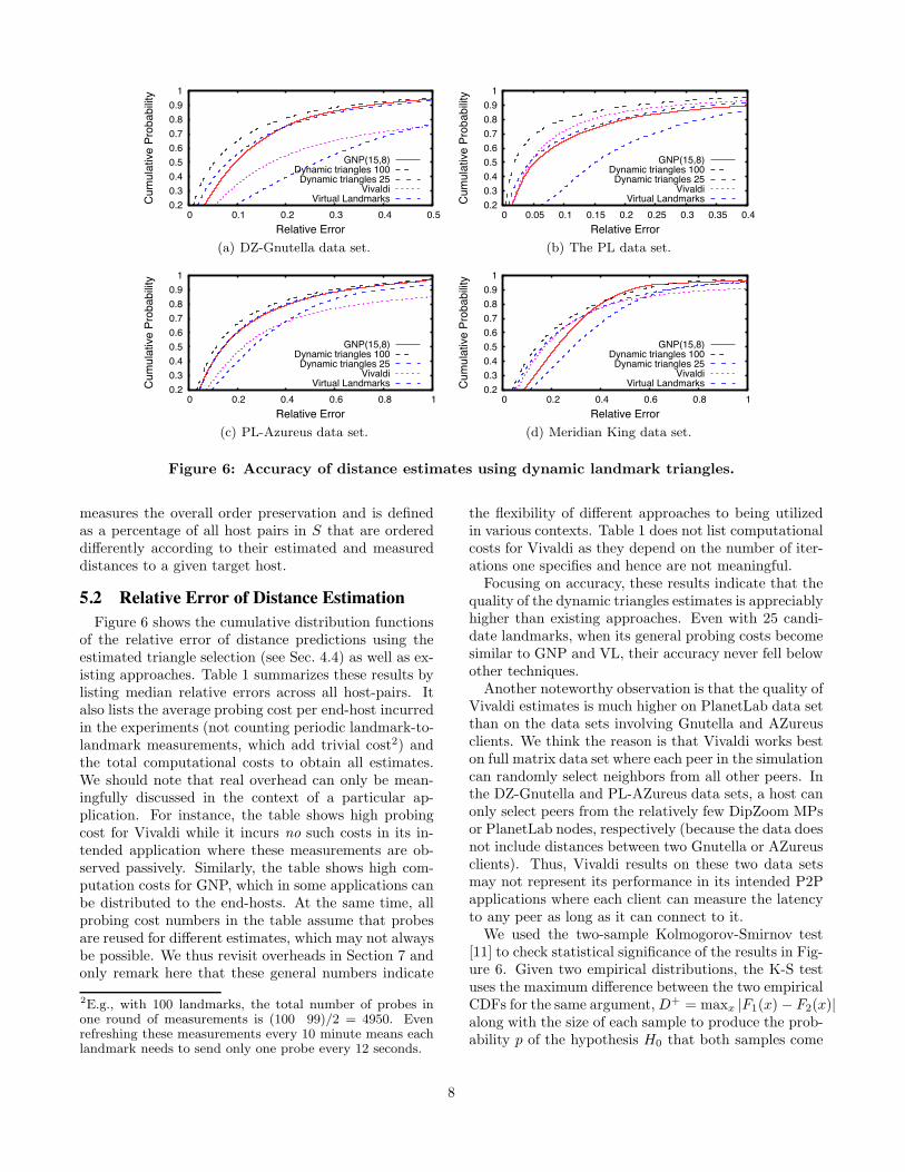
5.2 Relative Error of Distance EstimationFigure 6 shows the cumulative distribution functions

of the relative error of distance predictions using theestimated triangle selection (see Sec. 4.4) as well as ex-isting approaches. Table 1 summarizes these results bylisting median relative errors across all host-pairs. Italso lists the average probing cost per end-host incurredin the experiments (not counting periodic landmark-to-landmark measurements, which add trivial cost2) andthe total computational costs to obtain all estimates.We should note that real overhead can only be mean-ingfully discussed in the context of a particular ap-plication. For instance, the table shows high probingcost for Vivaldi while it incurs no such costs in its in-tended application where these measurements are ob-served passively. Similarly, the table shows high com-putation costs for GNP, which in some applications canbe distributed to the end-hosts. At the same time, allprobing cost numbers in the table assume that probesare reused for different estimates, which may not alwaysbe possible. We thus revisit overheads in Section 7 andonly remark here that these general numbers indicate

2E.g., with 100 landmarks, the total number of probes inone round of measurements is (100 99)/2 = 4950. Evenrefreshing these measurements every 10 minute means eachlandmark needs to send only one probe every 12 seconds.

the flexibility of different approaches to being utilizedin various contexts. Table 1 does not list computationalcosts for Vivaldi as they depend on the number of iter-ations one specifies and hence are not meaningful.Focusing on accuracy, these results indicate that the

quality of the dynamic triangles estimates is appreciablyhigher than existing approaches. Even with 25 candi-date landmarks, when its general probing costs becomesimilar to GNP and VL, their accuracy never fell belowother techniques.Another noteworthy observation is that the quality of

Vivaldi estimates is much higher on PlanetLab data setthan on the data sets involving Gnutella and AZureusclients. We think the reason is that Vivaldi works beston full matrix data set where each peer in the simulationcan randomly select neighbors from all other peers. Inthe DZ-Gnutella and PL-AZureus data sets, a host canonly select peers from the relatively few DipZoom MPsor PlanetLab nodes, respectively (because the data doesnot include distances between two Gnutella or AZureusclients). Thus, Vivaldi results on these two data setsmay not represent its performance in its intended P2Papplications where each client can measure the latencyto any peer as long as it can connect to it.We used the two-sample Kolmogorov-Smirnov test

[11] to check statistical significance of the results in Fig-ure 6. Given two empirical distributions, the K-S testuses the maximum difference between the two empiricalCDFs for the same argument,D+ = maxx |F1(x) − F2(x)|along with the size of each sample to produce the prob-ability p of the hypothesis H0 that both samples come

8

Methods Data Median Avg Comp.Set rel. error probes time

Tri 100 5.3% 55 13sTri 25 7.4% 13.5 7sGNP DZ-Gnu 9.6% 15 9mVL 23.5% 20 4 sec

Vivaldi 17 % 100 NATri 100 1.9 % 40 6sTri 25 4.2 % 14.4 5sGNP PL 5.3% 15 8mVL 15.1% 20 1s

Vivaldi 4.5 % 100 NATri 100 11.4 % 59 106sTri 25 14.2 % 13.7 19sGNP PL-Az 14.3% 15 8mVL 26.3% 20 10s

Vivaldi 22.6 % 100 NATri 100 13.8 % 51 228sTri 25 16.1 % 15.4 70sGNP Meridian 21.9 % 15 504mVL 28.6 % 20 42s

Vivaldi 17 % 100 NA

Table 1: Summary of estimation accuracy usingdifferent approaches on different data sets.

Methods Data D+-value p-valueSet

Tri/GNP 0.1941 < 2.2e− 16Tri/VL DZ-Gnu 0.4306 < 2.2e− 16

Tri/Vivaldi 0.3105 < 2.2e− 16Tri/GNP 0.2571 < 2.2e− 16Tri/VL PL 0.5367 < 2.2e− 16

Tri/Vivaldi 0.247 < 2.2e− 16Tri/GNP 0.0685 < 2.2e− 16Tri/VL PL-Az 0.2759 < 2.2e− 16

Tri/Vivaldi 0.2101 < 2.2e− 16Tri/GNP 0.1297 < 2.2e− 16Tri/VL Meridian 0.2614 < 2.2e− 16

Tri/Vivaldi 0.0786 < 2.2e− 16

Table 2: Statistical significance of the accuracydifferences.

0.2

0.3

0.4

0.5

0.6

0.7

0.8

0.9

1

0 0.1 0.2 0.3 0.4 0.5

Cum

ulat

ive

Pro

babi

lity

Relative Error

Dynamic trianglesGNP(15,8)

VivaldiVirtual Landmarks

Figure 7: Estimate accuracy for non-PlanetLabMPs.

0.2

0.3

0.4

0.5

0.6

0.7

0.8

0.9

1

0 0.1 0.2 0.3 0.4 0.5

Cum

ulat

ive

Pro

babi

lity

Relative Error

Hotz’s metric: LHotz’s metric: U

Hotz’s metric: (L+U)/2GNP(15,8)

Dynamic triangles

Figure 8: Accuracy of Hotz’s distance metrics.

from the same distribution, against the alternative hy-pothesis that they come from distinct distributions.Table 2 lists D+ and p values when testing empirical

distributions of triangle estimates vs. other estimatesfor each data set. We used the implementation of theK-S method in system R, where the smallest detected pvalue is 2.2e− 16. As we see for all data sets, the prob-ability that the distributions are the same is negligible(below the minimum detection level). Thus, with veryhigh probability, the alternative hypothesis – that thedistributions are different – is true, which in turn meansthat the accuracy advantage of dynamic triangles indi-cated by these distributions is statistically significant ineach of the environments represented by our data sets.Since three of our four datasets rely to varying ex-

tent on PlanetLab, we wished to validate our results byfocusing, in the DZ-Gnutella dataset, on the estimatesbetween the 21 non-PlanetLab MPs we had availableand the Gnutella peers. As shown in Figure 7, while ac-curacy of the non-PlanetLab estimates decreases some-what, it has similar trends. In particular, the medianerror of the dynamic triangle estimates becomes 7.4%as compared to 13.4% for GNP, 20% for Vivaldi and23.4% for virtual landmarks.

5.3 Early ApproachesThe GNP study [26] compared its accuracy to two

early approaches for distance estimation - IDMaps [7]and the Hotz’s approach [10] and found that these ap-

9

Error Tri GNP IDMaps Hotz’s U Hotz’s L Hotz’s (L+ U)/2Mean 15.9% 19.2% 29.5% 54.6% 60.3% 52.7%Median 5.3% 9.6% 13.0% 8.8% 11.4% 8.5%

Table 3: Mean and median relative error of early methods.

proaches were less accurate than GNP3. We checkedthis finding on the DZ-Gnutella dataset. Following themethodology in [26], we used the same 15 landmarksselected for GNP as Hotz’s landmarks so that both ap-proaches have the same probing overhead. At the sametime, because IDMaps is an asynchronous approach, weused all 100 landmarks we utilized for dynamic trian-gles. In the Hotz’s method, for a given host-pair, wecomputed the highest value of the lower-bound distanceestimate L and the lowest value of the upper-bound es-timate U produced by all the landmarks:

L =15

maxi=1

|d(A, hi)− d(B, hi)|

U =15

maxi=1

|d(A, hi) + d(B, hi)|where A and B are end-hosts, hi is the ith landmark,

and d(x, y) is the distance between hosts x and y. Wethen considered values L, U , and (L+U)/2 as alterna-tive distance estimates between the end-hosts.Table 3 compares the accuracy of these estimates

with those of GNP and dynamic trianges. IDMapsshows worse accuracy in terms of both median andmean error. Hotz’s heuristics actually show a slightadvantage over GNP in median errors but significantlylower overall average accuracy, indicating that it is vul-nerable to particularly bad estimates. Indeed, as Fig-ure 8, which depicts the CDF of the relative errors,indicates, there is a significant loss of accuracy of allthree Hotz’s metrics for the worst 20% of the estimates.These trends were confirmed in the other datasets: inthe PL dataset, Hotz’s metrics had slightly better me-dian but worse average errors similar to the DZ-Gnutelladataset above; in the PL-Azureous andMeridian datasetsboth median and mean errors in the Hotz’s methodwere worse that in GNP but the difference in the av-erage error was much more pronounced. Furthermore,all Hotz’s metrics showed lower accuracy than dynamictriangles for all the data sets and all error percentiles.Given these findings, we do not consider IDMaps and

Hotz metrics in the rest of our study.

5.4 Accuracy by Distance RangesLee et al. [16] observed that coordinate approaches

do not work well for estimating short distances due to

3To be fair, IDMaps had a goal of asynchronously collectingthe distance maps of the entire Internet and assumed manymore tracers than are available in our experiments, so both[26] and ours are not apple-to-apple comparisons.

0.01

0.1

1

10

<10ms 10-100ms >100ms

Rel

ativ

e er

ror

Real distance

GNP medianDynamic triangles median

Vivaldi medianVirtual landmarks median

Figure 9: Relationship between estimates accu-racy and inter-host distance.

large scale of triangle inequality violations. This sectionconsiders how the accuracy of our approach dependson the distance between the hosts. Figure 9 shows themedian relative errors for host-pairs that fall in severalreal distance ranges, for dynamic triangles and existingapproaches. We only show results for the DZ-Gnutelladata set; other data sets had similar results.This figure confirms the finding in [16], in that the

errors do increase significantly for estimating shorterdistances (note the logarithmic scale on Y-axis) for allmethods. For example, the median relative error of dis-tance prediction of GNP for real distance between 100and 1000 milliseconds is just under 10%, but it increasesto 68% for real distances below 10ms. (We also foundthat usually these estimates are biased to exceeding thereal distance.) The median relative error of distanceestimation of Vivaldi for the 100 to 1000ms range isonly about 11% and increases to over 700% for real dis-tances below 10 ms. Our approach also exhibits similarbehavior although to much less degree. The medianrelative error of our approach for real distances under10ms is only 17%, compared to GNP’s 68%. We be-lieve the reason behind this behavior is that, for shortinter-host distances, our approach finds a local trianglethat is close to both hosts while the coordinate-basedapproaches use the same host coordinates, derived fromthe same set of landmarks or peers, for all estimates re-gardless of the range. This, along with successful miti-gation of triangle inequality violations (see Section 3.2)limits the error produced by our approach.Within a limit, a somewhat higher relative error for

very short distance estimation may not be significantin practice (i.e., the difference between 2ms and 4msestimates might not be important as both indicate thatthe two hosts are “close”). However, the dependence of

10

estimation quality on distance ranges shown in Figure 9is noteworthy.

5.5 Rank PreservationAs already mentioned, in many applications, accurate

ranking of hosts according to their distance to a givenhost is more important than the accuracy of distanceestimations themselves. We now consider the two rankpreservation metrics [20] mentioned in Sec. 5.1 to studythe quality of dynamic triangle estimates in this respect.The results for the common closest peers are shown

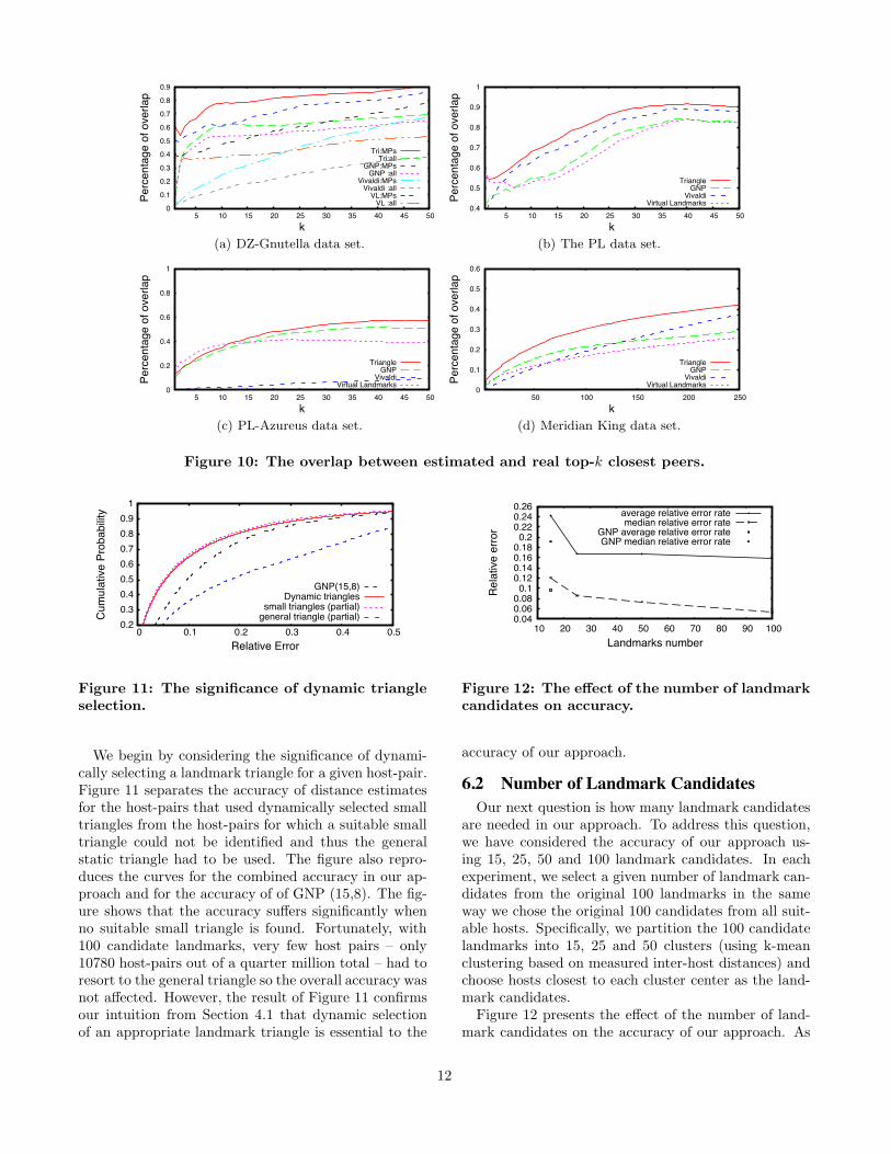
in Figure 10. To produce these plots, for each data set,we first compute the percentage of overlap of the k clos-est hosts to a given host X according to their estimatedand measured distances. The figure then plots the av-erage overlap found for all hosts X. In the DZ-Gnutellaand PL-Azureus data sets, we use, respectively, non-landmark DipZoom measurement points and PlanetLabnodes as hosts X relative to which the ranking is done.In the symmetrical PL and Meridian data sets, we useall non-landmark hosts as hosts X.With the DZ-Gnutella dataset, we additionally sepa-

rated our experiments in two groups. In one set of ex-periments, we only consider DipZoom measuring pointsas both the hosts to be ranked and the hosts relativeto which the ranking is done. In the other set, we con-sider the ranking of all hosts (both MPs and Gnutellapeers) relative to the MPs. The reason is that MPsare mostly deployed on well-connected PlanetLab nodeswhile Gnutella peers typically have residential connec-tivity. We included 220 available MPs in this studybeyond the 100 landmarks. However, some MPs lackedmeasured distances to some hosts, and hence the num-ber of hosts ranked relative to individual MPs may dif-fer.The results show that dynamic triangles have notice-

ably better rank preservation than the existing tech-niques in all data sets we considered. For example, inthe DZ-Gnutella data set, we found that in the MP-onlygroup, 125 out of 220 MPs had the same closest peerin both real and estimated distances, while this numberwas 113 for GNP estimations, 86 for virtual landmarksand only 8 for Vivaldi. (Thus, for k = 1, the graph gives0.57 for dynamic triangles, 0.52 for GNP, 0.39 for VL,and 0.036 for Vivaldi.) Considering the top-10 closestMPs, on average, 7.29 out of 10 closest peers predictedby dynamic triangles were among true top-10 closestpeers according to real distances; the same was true for6.06 out of 10 closest peers for GNP, 4.76 out of 10 forvirtual landmarks, and 2.45 out for 10 for Vivaldi. Inthe second group, where ranked hosts are dominated byresidential nodes, all methods showed accuracy degra-dation, especially for very low k, but dynamic trianglesstill retained an edge. We finally note that the rankpreservation of GNP according to the common closest

Method DZ-Gnutella DZ-Gnutella PL PL-AZ Meridian(MP-only) (All hosts)

TRI 5.83% 11.19% 5% 13.9% 21%GNP 9.35% 12.72% 8.4% 15.7% 24%VL 17.52% 28.3% 10.2% 19.2% 35.2%

Vivaldi 19.28% 24.2% 5.5% 19.3% 24.9%

Table 4: Relative rank loss

peers metric in our all-hosts experiment is similar tothat reported in the GNP study [26].Turning to the relative rank loss, Table 4 shows the

average value of this metric of different approaches inour data sets. In each data set, we computed this metricrelative to each available host and took the overall av-erage, for each approach. As seen from this table, whilethe relative rank loss of the dynamic triangles varies indifferent data sets, it is again always better than in theexisting approaches. Lua et al. [20] previously com-pared the relative rank loss of Vivaldi and the virtuallandmarks and they found their mean relative rank lossto be mostly between 15 and 20%.In summary, our rank preservation study shows that,

in addition to lower relative error, dynamic trianglesachieve better ranking accuracy than existing approaches,in many cases by a significant margin. Within the dy-namic triangles approach, as seen from results fromthe MP-only experiments on the DZ-Gnutella data setas well as from the PL data set, the top-1 selectionworks well when ranking well-connected hosts, pick-ing the true best host more than half the time. Atthe same time, the results from the from all-hosts inthe DZ-Gnutella data set and from PL-Azureous dataset indicate that top-1 selection performs much worsefor residential peers. However, the ranking accuracyof residential hosts increases rapidly towards top-10 se-lection. This behavior bodes well for peer-to-peer ap-plications, where top-1 selection is typically limited towell-connected super-peers while top-k selection oftenincludes other residential peers.

6. DESIGN ISSUESWe now examine the effect of several design and con-

figuration issues on the accuracy of the dynamic triangleestimates. In particular, we consider the significance ofdynamic triangle selection (vs. using a common big tri-angle for all host-pairs), the effect of the number of can-didate landmarks on the accuracy of the approach, theimpact of triangle inequality violations, the impact ofusing the estimated host-to-landmark distances in tri-angle selection, and the effect of our heuristic for choos-ing the initial value of the threshold described in Sec-tion 3. We used the DZ-Gnutella data set for all theexperiments in this section.

6.1 Impact of Dynamic Triangle Selection

11

0

0.1

0.2

0.3

0.4

0.5

0.6

0.7

0.8

0.9

5 10 15 20 25 30 35 40 45 50

Per

cent

age

of o

verla

p

k

Tri:MPsTri:all

GNP:MPsGNP :all

Vivaldi:MPsVivaldi :all

VL:MPsVL :all

(a) DZ-Gnutella data set.

0.4

0.5

0.6

0.7

0.8

0.9

1

5 10 15 20 25 30 35 40 45 50

Per

cent

age

of o

verla

p

k

TriangleGNP

VivaldiVirtual Landmarks

(b) The PL data set.

0

0.2

0.4

0.6

0.8

1

5 10 15 20 25 30 35 40 45 50

Per

cent

age

of o

verla

p

k

TriangleGNP

VivaldiVirtual Landmarks

(c) PL-Azureus data set.

0

0.1

0.2

0.3

0.4

0.5

0.6

50 100 150 200 250

Per

cent

age

of o

verla

p

k

TriangleGNP

VivaldiVirtual Landmarks

(d) Meridian King data set.

Figure 10: The overlap between estimated and real top-k closest peers.

0.2

0.3

0.4

0.5

0.6

0.7

0.8

0.9

1

0 0.1 0.2 0.3 0.4 0.5

Cum

ulat

ive

Pro

babi

lity

Relative Error

GNP(15,8)Dynamic triangles

small triangles (partial)general triangle (partial)

Figure 11: The significance of dynamic triangleselection.

We begin by considering the significance of dynami-cally selecting a landmark triangle for a given host-pair.Figure 11 separates the accuracy of distance estimatesfor the host-pairs that used dynamically selected smalltriangles from the host-pairs for which a suitable smalltriangle could not be identified and thus the generalstatic triangle had to be used. The figure also repro-duces the curves for the combined accuracy in our ap-proach and for the accuracy of of GNP (15,8). The fig-ure shows that the accuracy suffers significantly whenno suitable small triangle is found. Fortunately, with100 candidate landmarks, very few host pairs – only10780 host-pairs out of a quarter million total – had toresort to the general triangle so the overall accuracy wasnot affected. However, the result of Figure 11 confirmsour intuition from Section 4.1 that dynamic selectionof an appropriate landmark triangle is essential to the

0.04 0.06 0.08

0.1 0.12 0.14 0.16 0.18

0.2 0.22 0.24 0.26

10 20 30 40 50 60 70 80 90 100

Rel

ativ

e er

ror

Landmarks number

average relative error ratemedian relative error rate

GNP average relative error rateGNP median relative error rate

Figure 12: The effect of the number of landmarkcandidates on accuracy.

accuracy of our approach.

6.2 Number of Landmark CandidatesOur next question is how many landmark candidates

are needed in our approach. To address this question,we have considered the accuracy of our approach us-ing 15, 25, 50 and 100 landmark candidates. In eachexperiment, we select a given number of landmark can-didates from the original 100 landmarks in the sameway we chose the original 100 candidates from all suit-able hosts. Specifically, we partition the 100 candidatelandmarks into 15, 25 and 50 clusters (using k-meanclustering based on measured inter-host distances) andchoose hosts closest to each cluster center as the land-mark candidates.Figure 12 presents the effect of the number of land-

mark candidates on the accuracy of our approach. As

12

Num. of violations 0 1 2 3Prevalence 25.7% 34.3% 22.1% 17.8%

Median rel. error 4.2% 5.2% 5.7% 6.7%

Table 5: the degree of triangle inequality viola-tions and its effect on accuracy.

0.2

0.3

0.4

0.5

0.6

0.7

0.8

0.9

1

0 0.1 0.2 0.3 0.4 0.5

Cum

ulat

ive

Pro

babi

lity

Relative Error

GNP(15,8)Dynamic triangles (measured)Dynamic triangles (estimated)

Figure 13: Estimated vs. measured triangle se-lection.

we can see, both the average and median relative errorrate decrease as the number of candidate landmarks in-creases from 15 to 100, as host-pairs are more likely tofind an acceptable small triangle. However, the decreaseis most significant for low numbers (15-25) of land-marks. This result is encouraging because it suggeststhat high-quality distance estimates can be achieved bymaintaining a relatively limited set of landmarks. Cer-tainly 100 landmark candidates used in our study is ad-equate, and fewer numbers can be sufficient dependingon the application.

6.3 Triangle Inequality ViolationsTurning to the impact of triangle inequality viola-

tions, their effect on accuracy of our approach is shownin Table5. For a given pair of end-hosts and the selecteddynamic triangle, the number of triangle violations inour approach could range from 0 to 3 (Section 3.2), andmost host-pairs had at least some violations. As onewould expect, we found a direct dependence betweenthe number of violations and the inaccuracy of the dis-tance estimation for a given host-pair. However, theloss of accuracy is modest, ranging from 4.2% for no vi-olations to 6.7% for three violations. We conclude thatour approach successfully mitigates the effect of triangleinequality violations.

6.4 Using Estimated Distances in Triangle Se-lection

Our approach selects the best landmark triangle for agiven host-pair based on the estimated distance betweenthese hosts and all landmark candidates. To considerhow much accuracy is lost due to using estimated dis-tances in triangle selection, Figure 13 compares the ac-curacy of the estimates produced by our triangle selec-

tion with the selection using measured distances. Recallfrom Section 4.4 that the latter is an idealistic methoddue to its prohibitive probing traffic. Fortunately, asthe figure shows, the use of estimated distances in tri-angle selection does not lead to considerable accuracyloss. The selection based on measured distances has themedian error of 4.7% compared to 5.3% in the selectionusing estimated distances.

7. APPLICATIONSWhile accuracy of distance estimates is important,

their true utility transpires in the context of specificapplications using them. In this section, we evaluateour approach when used for two representative typesof applications - host clustering and content deliverynetworks.

7.1 Host ClusteringAn important application of distance estimation is

host clustering, which is used in a large variety of con-texts, including peer-to-peer systems, scalable networkmonitoring, and content dissemination. Pair-wise dis-tance measurements between nodes would ideally driveclustering algorithms but are often unavailable, eitherdue to the system size (since the number of measure-ments grows quadratically with the number of nodes),or because of the lack of control over the nodes. Inthese cases, distance estimates provide a viable alter-native, and have been used, e.g., by Chen et al. inthe context of network monitoring [2]. We evaluate dis-tance estimation techniques with respect to clusteringby considering how clusters formed using estimates pro-vided by the corresponding approach deviate from clus-ters formed using true measured distances.We again used DZ-Gnutella dataset for this exper-

iment. We selected 99 non-landmark MPs for whichwe have the complete matrix of real (i.e., measured)inter-MP distances and used the k-mean clustering algo-rithm to group them into five clusters. To compare thereal-distance clustering with a given estimated-distanceclustering, we pair up clusters from each clustering thathave the largest number of nodes in common; we thencompute the total number of mismatched nodes acrossall cluster pairs. We consider two dynamic triangleconfigurations - with 100 and 25 landmark candidates.Note that Vivaldi is intended for peer-to-peer applica-tions; it would not be used for pure clustering and isincluded in this study for completeness.Table 6 shows the performance results. We see that

dynamic triangle estimates produce the highest qualityclusters, with only 5 out 99 nodes mismatched. Thisfollowed by GNP, but dynamic triangle incurred dras-tically lower computational cost to produce all the dis-tance estimates than GNP. Virtual landmarks had thelowest computational overhead (we measured it with a

13

Method Computation mismatched Median Networktime nodes rel error probings

TRI 100 2 sec 5 2.2% 4546TRI 25 1 sec 5 4.5% 1187GNP 6 min 11 7.3% 1485VL < 1 sec 20 29% 1980

Vivaldi NA 17 18.3% 9900

Table 6: Host clustering performance

second granularity and their overhead was below ourability to measure).To measure the probing overhead, we counted the

actual number of probes required in each approach toproduce all the distance estimates. As explained earlier,we only count the number of probes between the land-marks and hosts, because the periodic probes amongthe landmarks are negligible. Dynamic triangles with100 landmarks generate three times more probes thanGNP; the reason is that, although we use fewer probesfor each estimate, the same host may probe differenttriangles for different estimates while a host in GNPalways reuses its probes.Interestingly, our approach produced identical clus-

ters using 25 and 100 landmarks, although going from100 to 25 landmarks doubled the median relative errorof inter-host distance estimates. With 25 probes, dy-namic triangles actually generated slightly lower prob-ing traffic than GNP. This shows that in some scenar-ios, one can reduce the costs of the estimates withoutsacrificing their value. Systematic ways to exploit thispotential for optimization is an interesting question forfuture work.Overall, while these results are based only on one set

of hosts and should be viewed as preliminary, dynamictriangle estimations produced better-quality clusters thanGNP in this case.

7.2 CDN Server SelectionAnother appealing application of network distance es-

timation is to use it for server selection in a contentdelivery network (CDN). While even efficient estimateswould be too heavy-weight for online server selectionin the context of delivering small HTTP objects, CDNsare increasingly used to deliver large files (such as soft-ware packages and multimedia files) and long-runningstreaming media. With dynamic triangles being able toestimate 10,000 distances in single seconds (see Table 6)this clearly makes it feasible to use online distance es-timates in server selection in these contexts.Recently, Szymaniak et al. [30] studied the applica-

tion of GNP estimates to select among ten servers inthe Google content delivery network and found themquite effective. We consider the application of dynamictriangle estimates to a large-scale CDN, using Akamaiwith its thousands of servers as a target environment.

In this section, we first compare the performance of ourestimates in this application with existing approachesusing a simulation study on a data set employed in theoriginal Meridian study [35]. We then report the resultsfrom a live Internet experiment that measures the qual-ity of server selection in the Akamai platform by thedynamic triangles and GNP.

7.2.1 Simulation Study

We now compare the quality of server selection us-ing dynamic triangle estimates with several alternativetechniques that have been proposed for this purpose– GNP, Vivaldi, and Meridian. We use the MeridianKing data set and follow the general methodology ofMeridian study in this experiment. In particular, weare interested in the general quality of server selectionpromised by each approach, thus assuming a speciallymodified Web client. We use the absolute value of thedifference in distance from a client to its true closestserver and from the same client to the server selectedby a given approach, as the measure of quality of theapproach.The Meridian King data set [23] contains the dis-

tance between 2500 local DNS servers collected usingKing method. We randomly pick 500 nodes as CDNclients and apply different techniques to select the clos-est server among the remaining 2000 nodes. In the caseof dynamic triangles, we use one-sided triangle selectionas discussed in Section 4.3.The original median absolute difference in our ap-

proach is 12.3ms, which is similar to the results us-ing (15,8)-GNP and Vivaldi in the Meridian study [35]and much higher than the Meridian system, i.e., about1.3ms observed from Figure 8 in [35]. However, Merid-ian’s accuracy comes with a high probing cost. Accord-ing to [35], the average bandwidth cost for each closestserver discovery is 10.4KBytes with a probe packet sizeof 50 bytes. This translates to 104 probes if we assumeeach probe generates two packets. As mentioned in theMeridian study, with this “budget” of active probes,other techniques could improve their selection qualityby using distance estimates only to predict top-k can-didate closest servers and actively probing all these kservers to arrive at the final selection.Figure 14 compares Meridian server selection with

that of GNP, Vivaldi and our approach with this op-timization, for different sizes k of the candidate serverset. It shows that the median absolute difference dropssharply as k increases for all three approaches using dis-tance estimates, especially in our case. For k = 10, thequality of our approach reaches the Meridian’s, whileour system only uses 6+10=16 probes and Meridianuses over 100 probes on average. For higher values of k,the quality of our approach improves beyond the Merid-ian’s level while the total probing cost of our approach

14

0 2 4 6 8

10 12 14 16 18

1 10 100

Abs

oulte

diff

eren

ce (

ms)

Number of active probings

TrianglesGNP(15,8)

VivaldiMeridian

Figure 14: The absolute difference for closestservers selection with active probings.

is still lower than Meridian.The above cost analysis does not include maintenance

costs, but these costs are negligible (compared to thecost of content delivery to clients) and similar in bothsystems. For dynamic triangles, the full complementof maintenance measurements includes pair-wise probesbetween all landmarks as well as between landmarksand servers. With 2000 servers and 100 landmarks, thistranslates into 2000 ∗ 100+100 ∗ 99/2 = 204950 probes.For Meridian, each server probes servers in its rings. Inthe experiment of Figure 14, a server has nine rings andup to 16 servers in each ring [35], for roughly 2000 ∗(9 ∗ 16) = 288000 probes. Allowing for some probereuse and some rings having fewer servers, this resultsin roughly similar maintenance costs.

7.2.2 A Live Internet Experiment

To compare our approach with GNP in a realistic set-ting, we implemented an AJAX application that, whenloaded by a client, performs server selection among Aka-mai edge servers using dynamic triangles, GNP, andAkamai itself, and reports to us the latency from theclient to each of the three servers. Following [30], weused GNP(7,6) configuration in this study. We picked aCNAME (a1694.g.akamai.net, utilized by pcworld.com)which we found is mapped by Akamai to a large numberof edge servers, 979. We request a bogus URL from theselected server in all cases, receiving a short “Bad Re-quest” response. We verified through tcpdumps on ourown client that downloading this response involves tworound-trip times (RTTs) between the client and server.We have maintained about 90 landmark servers on

the PlanetLab platform (we attempt to maintain up to104 but the actual number varies due to the instabilityof PlanetLab nodes). We keep the complete distancematrix between all the landmarks as well as betweeneach landmark and each of the 979 Akamai server. Weselect (through clustering as described in Section 5.1)three of these landmarks as the general big trianglefor our approach, and seven landmarks for GNP(7,6).Given the instability of PlanetLab nodes, we select, for

each of the above landmarks, a few nearby landmarksas backups.We implemented three Web pages, one for each server

selection. The Akamai page includes Javascript thatsimply accesses a bogus URL with the above CNAME,thus following the Akamai server selection, and reportsthe response time to our server. To factor out DNSresolution time, we perform the download twice andreport the second measurement.The triangles page4 embeds three images with URLs

pointing to the landmarks at the vertexes of the big tri-angle5. As the client establishes the TCP connectionsto these landmarks, they passively measure RTT to theclient, select a small triangle based on these measure-ments6, and then respond to the client with an HTTPredirect to three URLs pointing to the vertexes of thesmall triangle. The latter landmarks similarly measureRTT to the client, estimate the distance from the clientto all 979 Akamai servers and select the best one. Fi-nally, one of the landmarks returns a redirect to theselected server using its raw IP address (and a bogusURL) while the other two landmarks return an emptyimage. The client follows the redirect and reports thedownload time to our server.The GNP page7 is implemented similarly but embeds

seven images (to measure RTT to the seven landmarks)and involves one round of landmark communicationsinstead of two.We asked a commercial company to embed zero-sizes

iframes with the above three pages, and we also embed-ded them into our own Web pages. We have collected24,079 measurements from 2,926 distinct client IP ad-dresses, representing 47 US states and 43 foreign coun-tries according to the GeoIP database from MaxMind[22].Figure 15 shows the CDF of the measured RTT from

clients to Akamai servers selected by the three methods,and Table 7 lists their median and mean values. Theseresults show the performance of the dynamic triangles issignificantly better than GNP(7,6), with almost a factorof two reduction in median client-to-server RTT (32msvs 62.4ms). It is well established that latency directlyaffects TCP throughput (see, e.g., [27]) and hence thislatency reduction would translate directly into the re-duction in web page download time as experienced bythe user. In fact, the server selection quality with oursimple technique is fairly close to that of Akamai it-self, despite Akamai’s extensive Internet-wide measure-

4See http://haddock.case.edu:8000/triangle.5This is a slight simplification. In fact, these URLs point toour portal server which uses HTTP redirect to to send theclient to the landmarks. This level of indirection allows usto replace failed landmarks with their backup dynamically.6This and other actions requiring central computation aredone through a back-end server.7See http://haddock.case.edu:8000/gnp.

15

Method Median RTT (ms) Mean RTT(ms)Akamai 24.8 52.4Triangle 32 62.4

(7,6) GNP 62.4 88.5

Table 7: Performance of closest CDN server se-lection for web clients.

0

0.2

0.4

0.6

0.8

1

0 100 200 300 400 500

Cum

ulat

ive

Pro

babi

lity

Distance to the selected best Akamai server (ms)

TrianglesGNP(7,6)

Akamai

Figure 15: The quality of CDN server selectionin a live deployment.

ments and network topology expertise that go into itsserver selection decisions [17, 18]. By adding a few ac-tive probes to top-k servers as described in Section 7.2.1,we hope to be able to close this gap in the future.At the same time, dynamic triangles require 6 probes

for each server selection vs. 7 probes needed by GNP(7.6).These 6 probes do come in two sequential rounds whileGNP sends all its probes in parallel. However, for largedownloads we are targeting, finding a better server islikely to be worth this small initial delay.

8. CONCLUSIONThis paper presents a simple and efficient approach

for estimating the network distance between Internethosts. Our approach uses a set of hosts that act aslandmark candidates, and dynamically selects a trian-gle of landmarks for a given pair of hosts that are likelyto produce high-accuracy distance estimates. Once thelandmark triangle is selected, the estimate is computedfrom a simple trigonometrical calculation. Through ex-tensive testing we showed that our approach comparesfavorably with representative existing methods for dis-tance estimation, both from the general accuracy andoverhead perspective and in the context of some specificapplications.We are currently implementing our approach in the

BitTorrent tracker and Vuze client. As future work,we would like to investigate some optimizations to ourapproach we mentioned throughout the paper, most no-tably, accounting for triangle shape during dynamic tri-angle selection and using a replacing the triangle witha single landmark when it is particularly close to one ofthe end hosts. We would also like to combine our ap-proach with some orthogonal techniques that have been

proposed to enhance distance estimation and measure-ment [15, 16].

Appendix A: Trigonometric DerivationsAssume we have 3 landmarks L1,L2 and L3 and twopoints A and B. We also know the distance betweenlandmarks and their distance to points A and B, and weneed to find the distance between A and B. In the for-mulas below, we use P1, P2 to denote the edge betweenpoints P1 and P2 and |P1, P2| to denote its length. Weuse ∠(P1, P2, P3) to denote the angle between edgesP1, P2 and P2, P3.Points A and B each can have two possible positions,

A′, A′′, B′ and B′′ as illustrated in Figure 1 and 2. Sincewe know the length of edges A,L1, A,L2, and L1, L2,we can calculate the cosine of angle ∠(A,L1, L2) usingthe following triangle function, regardless of whether Ais positioned at A′ or A′′:

cos∠(A,L1, L2) =|A,L1|2 + |A,L2|2 − |L1, L2|2

2 ∗ |A,L1| ∗ |A,L2| (1)

We can obtain the cosine of angle ∠(B,L1, L2) usingthe same method. As the next step, we would like tofind the cosine of ∠(A,L1, B). However, depending onwhether or not points A and B are on the same side online L1, L2, angle ∠(A,L1, B) can be the sum of twoangles ∠(A,L1, L2) and ∠(B,L1, L2), or the differencebetween these angles. Thus, its cosine will be:

cos∠(A,L1, B) = cos(∠(A,L1, L2)± ∠(B,L1, L2))

= cos∠(A,L1, L2) ∗ cos∠(B,L1, L2)

∓ sin∠(A,L1, L2) ∗ sin∠(B,L1, L2) (2)

where we use the upper arithmetic operation if A andB are on the same side on line L1, L2 and the lowerarithmetic operation otherwise.In order to determine whether A and B are on the

same side of L1, L2, we utilize point L3 as a witnesspoint. First, we determine if A and L3 are on the sameside of line L1, L2 or not. To this end, we obtain thecosines of angles ∠(A,L1, L2) and ∠(L3, L1, L2) usingthe equation similar to 1, and use these cosine values tocompute the two possible cosine values of ∠(A,L1, L3)using the equation similar to 2. We also obtain thecosine of ∠(A,L1, L3) directly from the edges, usingequation similar to 1 and compare it to the two valuesfound from 2. Depending on which of these two valuesare closer, we conclude whether A and L3 are on thesame side of line L1, L2 or not. We repeat the samemethod to determine whether or not points B and L3are on the same or opposite sides of L1, L2. We thencan answer our question on the post ion of points Aand B relative to L1, L2: if both A and B are on thesame side with L3, or both are on the opposite side fromL3, then both A and B are on the same side of L1, L2.Otherwise, they will be on the opposite sides of L1, L2.

16

Finally, we can use the above conclusion to chose be-tween the two alternative values of cos∠(A,L1, B) and,knowing now this cosine value, calculate the estimateddistance between A and B using the following equation3:

|A,B|2 = |A,L1|2 + |B,L1|2 + 2|A,L1||B,L1| cos∠(A,L1, B)(3)

9. REFERENCES[1] Akamai Technologies.

http://www.akamai.com/html/technology/index.html.[2] Y. Chen, K. H. Lim, R. H. Katz, and C. Overton. On the

stability of network distance estimation. Perf. Eval. Rev.,30(2):21–30, 2002.

[3] M. Costa, M. Castro, A. Rowstron, and P. Key. PIC:Practical Internet coordinates for distance estimation. InICDCS, 2004.

[4] F. Dabek, R. Cox, F. Kaashoek, and R. Morris. Vivaldi: adecentralized network coordinate system. In SIGCOMM,2004.

[5] DipZoom. http://dipzoom.case.edu.[6] http://vorlon.case.edu/∼zxw20/distance/.[7] P. Francis, S. Jamin, C. Jin, Y. Jin, D. Raz, Y. Shavitt,

and L. Zhang. IDMaps: a global Internet host distanceestimation service. IEEE/ACM Trans. Netw.,9(5):525–540, 2001.

[8] GNP. www.cs.rice.edu/∼eugeneng/research/gnp.[9] K. Gummadi, S. Saroiu, and S. Gribble. King: Estimating

latency between arbitrary internet end hosts. InSIGCOMM Internet Measurement Workshop, 2002.

[10] S. M. Hotz. Routing information organization to supportscalable interdomain routing with heterogeneous pathrequirements. Ph.d. thesis, University of SouthernCalifornia, 1994.

[11] F. James. Statistical Methods in Experimental Physics (2ndEdition). World Scientific, 2006.

[12] J. Jung, B. Krishnamurthy, and M. Rabinovich. Flashcrowds and denial of service attacks: characterization andimplications for CDNs and Web sites. In Proc. 8th Int.Conf. on WWW, 2002.

[13] B. Krishnamurthy and J. Wang. On network-awareclustering of web clients. In SIGCOMM, 2000.

[14] J. Ledlie, P. Gardner, and M. Seltzer. Network coordinatesin the wild. In NSDI ’07.

[15] J. Ledlie, P. Pietzuch, and M. Seltzer. Stable and accuratenetwork coordinates. In ICDCS ’06.

[16] S. Lee, Z.-L. Zhang, S. Sahu, and D. Saha. On suitability ofeuclidean embedding of internet hosts. Perf. Eval. Rev.,2006.

[17] F. T. Leighton, R. Sundaram, and M. Levine. Method forgenerating a network map. Akamai Technologies, Inc. USPatent No.: 7,251,688.

[18] M. Levine, R. Kleinberg, and A. Soviani. Method forextending a network map. Akamai Technologies, Inc. USPatent No.: 7,028,083.

[19] H. Lim, J. C. Hou, and C.-H. Choi. Constructing internetcoordinate system based on delay measurement.IEEE/ACM Trans. Netw., 13(3):513–525, 2005.

[20] E. K. Lua, T. Griffin, M. Pias, H. Zheng, and J. Crowcroft.On the accuracy of embeddings for Internet coordinatesystems. In IMC’05.

[21] C. Lumezanu, R. Baden, N. Spring, and B. Bhattacharjee.Triangle inequality and routing policy violations in theinternet. In PAM, pages 45–54, 2009.

[22] MaxMind. http://www.maxmind.com.[23] Meridian: Lightweight positioning.

http://www.cs.cornell.edu/People/egs/meridian/.[24] Network coordinate research at harvard.

http://www.eecs.harvard.edu/∼syrah/nc/.

[25] T. S. E. Ng and H. Zhang. A network positioning systemfor the internet. In ATEC’04.

[26] T. S. E. Ng and H. Zhang. Predicting internet networkdistance with coordinates-based approaches. In INFOCOM,2002.

[27] J. Padhye, V. Firoiu, D. F. Towsley, and J. F. Kurose.Modeling tcp reno performance: a simple model and itsempirical validation. IEEE/ACM Trans. Netw.,8(2):133–145, 2000.

[28] M. Pias, J. Crowcroft, S. Wilbur, S. Bhatti, and T. Harris.Lighthouses for scalable distributed location. In IPTPS,2003.

[29] Y. Shavitt and T. Tankel. Big-bang simulation forembedding network distances in euclidean space.IEEE/ACM Trans. Netw., 12(6):993–1006, 2004.

[30] M. Szymaniak, D. Presotto, G. Pierre, and M. van Steen.Practical large-scale latency estimation. Comput. Netw.,52(7):1343–1364, 2008.

[31] L. Tang and M. Crovella. Virtual landmarks for theInternet. In IMC’03.

[32] Z. Wen. Simplifying End-to-End Mesurement on theInternet. PhD thesis, Case Western Reserve University,2009.

[33] Z. Wen and M. Rabinovich. Network distance estimationwith dynamic landmark triangles (Poster paper). InSIGMETRICS, 2008.

[34] Z. Wen, S. Triukose, and M. Rabinovich. Facilitatingfocused internet measurements. In SIGMETRICS, 2007.

[35] B. Wong, A. Slivkins, and E. G. Sirer. Meridian: alightweight network location service without virtualcoordinates. In SIGCOMM05, 2005.

[36] B. Zhang, T. S. E. Ng, A. Nandi, R. H. Riedi, P. Druschel,and G. Wang. Measurement based analysis, modeling, andsynthesis of the internet delay space. In InternetMeasurement Conference, pages 85–98, 2006.

[37] H. Zheng, E. K. Lua, M. Pias, and T. G. Griffin. Internetrouting policies and round-trip-times. In PAM, pages236–250, 2005.

17