dynamic light scattering pcs) - harvard university · dynamic light scattering pcs) interference...
TRANSCRIPT

Dynamic Light Scattering(aka QLS, PCS)
Oriented particles create interference patterns, each bright spot being a speckle. The speckle pattern moves as the particle move, creating flickering.
All the motions and measurements are described by correlations functions• G2(!)- intensity correlation function describes particle motion• G1(!)- electric field correlation function describes measured fluctuations
Which are related to connect the measurement and motion
Analysis Techniques:• Treatment for monomodal distributions: linear and cumulant fits• Treatment for non-monomodal distributions: Contin fits
It is also possible to measure other motions, such as rotation.
"#$
%&' ()
22 11 )(gB)(G !*!

2
Particles behave like ‘slits’, the orientation of which generates interference patterns
Generates a ‘speckle’ pattern
Various points reflect different scattering angles

Movement of the particles cause fluctuations in the pattern
The pattern ‘fluctuates’
Movement is defined by the rate of fluctuation

Measure the intensity of one speckle
Experimentally, the intensity of one ‘speckle’ is measured

Order of magnitude for time-scale of fluctuations
+ , Dtx )- 2
fluctuations occur on the time-scale that particles move about one wavelength of light…
Assuming Brownian motion of the particles…
The time-scale is:
./-x
+ , secms/cmx.
cmxt 1001052105
28
25// 0
0
D for ~ 200 nm particles
. ~ 500 nmChange on the
msec time frame

1. Measure fluctuations an convert into an Intensity Correlation Function
2. Describe the correlated movement of the particles, as related to particle size into an Electric-Field Correlation Function.
3. Equate the correlation functions, with the Seigert Relationship
How is the time scale of the fluctuations related to the particle movement?
Requires several steps:
4. Analyze data using cumulants or CONTIN fitting routines

• Math/Theory
• Application/Optics
• Data Analysis
2 texts:
‘Light scattering by Small Particles’ by van de Hulst
‘Dynamic Light Scattering with applications to Chemistry, Biology and Physics’ by Berne and Pecora

+ , !!! dtI)t(IT
)(G T (1) 021
First, the Intensity Correlation Function, G2(!)
I(t) I(t+!)
Describes the rate of change in scattering intensity by comparing the intensity at time t to the intensity at a later time (t + !), providing a quantitative measurement of the flickering of the light
Mathematically, the correlation function is written as an integral over the product of intensities at some time and with some delay time, !
Which can be visualized as taking the intensity at I(t) times the intensity at I(t+!)- red), followed by the same product at I(t+t’)-blue, and so on…
I(t+!’)

Tau (2sec)
1 10 100 1000
G 2( !
)
8.0e+7
1.0e+8
1.2e+8
1.4e+8
1.6e+8
1.8e+8
Tau (2sec)
0 1000 2000 3000 4000 5000
G 2( !
)
8.0e+7
1.0e+8
1.2e+8
1.4e+8
1.6e+8
1.8e+8
The Intensity Correlation Function has the form of an exponential decay
plot linear in !
plot logarithmic in !
The correlation function typically exhibits an exponential decay

Instead, we correlate the motion of the particles relative to each other
It is Not Possible to Know How Each Particle Moves from the Flickering
Second, Electric Field Correlation Function, G1(!)

+ , !!! dtE)t(ET
)(G T (1) 011
Integrate the difference in distance between particles, assuming Brownian Motion
The electric field correlation function describes correlated particle movement, and is given as:
!! 30) exp)(G1
G1(t) decays as and exponential with a decay constant 345for a system undergoing Brownian motion
Constructive interference
Destructive interference

The decay constant is re-written as a function of the particle size
ichydrodynammicthermodyna
6))r
kTD62
Boltzmann Constant
temperature
viscosity particle radius
with q2 reflecting the distance the particle travels … and the application of Stokes-Einstein equation
2Dq0)3
The decay constant is related by Brownian Motion to the diffusivity by:
789
:;<)
24 =.6 sinnq

Tau
1e-6 1e-5 1e-4 1e-3 1e-2 1e-1
G 2(!
)
0.0
0.1
0.2
0.3
0.4
0.5
0.6
0.7
0.8
0.9
1.0
Tau
0.000 0.002 0.004 0.006 0.008 0.010 0.012
G 2(!
)
0.0
0.1
0.2
0.3
0.4
0.5
0.6
0.7
0.8
0.9
1.0
large particle
small particle
Rate of decay depends on the particle size
large particles diffuse slower than small particles, and the correlation function decays at a slower rate.
and the rate ofother motions
(internal, rotation…)

"#$
%&' ()
22 11 )(gB)(G !*!
Finally, the two correlation function can be equated using the Seigert Relationship
Intensity Correlation Function(recall: this is measured)
Electric Field Correlation Function(recall: this is what the particles are doing)
where B is the baseline and * is an instrumental response, both of which are constants
The Seigert Relationship is expressed as:
Based on the principle of Guassian randomprocesses – which the scattering light usually is
*2E IIntensity EE >))

• G2(!) intensity correlation function measures change in the scattering intensity
• G1(!) electric field correlation function describes correlated particle movements
• The Seigert Relationship equates the functions connecting the measurable to the motions
"#$
%&' ()
22 11 )(gB)(G !*!

• Math/Theory
• Application/Optics
• Data Analysis

So, consider a simple example of the process
Measure the intensity fluctuations from a dispersion of particles.

Commercial Equipment• Need laser, optics, correlator, etc…
• Commercial Sources– Brookhaven Instruments – Malvern Instruments – Wyatt Instruments
(multiangle measurements, HPLC detectors)– ALV (what we have)
• Costs range $50K to $100K

Instrumental Considerations• Light Source
– Monochromatic, polarized and continuous (laser)– Static light scattering goes as 1/!4, suggests shorter
wavelengths give more signal• typical Ar+ ion laser at 488 nm
– Dynamic light scattering S/N goes as !, while detector sensitivity goes as 1/!, so wavelength is not too critical. HeNe lasers are cheap and compact, but weaker (! = 633 nm)
– Power needed depends on sample (but there can be heating!)– Calculation of G(") depends on two photons, and so on the
power/area in the cell. Typically focus the beam to about 200 #m
– Sample can be as small as 1 mm in diameter and 1 mm high. Typical volumes 3-5 ml.

Instrument Considerations• Need to avoid noise in the correlation functions
– Dust! • Usually adds an unwanted (slow) component• See in analysis – some software help• AVOID by proper sample preparation when possible
– Poisson Noise• counting noise, decreases with added counts, important to have
enough counts; typically 107 over all with 106 at baseline
– Stray light• adds an unwanted heterodyne component (exp (-$) instead of
exp (-2$). Avoid with proper design

Correlators• Need to calculate
which is approximated by
so calculate by recording I(t) and sequentially multiplying and adding the result. To do in real time requires about ns calculations thus specialized hardware
• Pike – 1970s (Royal Signals and Radar Establishment, Malvern, England)
• Langley and Ford (UMASS) ? Brookhaven• 1980’s Klaus Schatzel, Kiel University ? ALV
+ , !!! dtI)t(IT
)(G T (1) 021
)()(1)()arg(
12 !! (/ @
)i
elN
ii tItI
NG

Autocorrelation function is collected
2.000000000E+000 1.593461120E+0082.400000095E+000 1.590897440E+0085.000000000E+000 1.582029760E+0081.000000000E+001 1.564198880E+0081.500000000E+001 1.546673760E+0082.000000000E+001 1.529991520E+0082.500000000E+001 1.513296000E+0083.000000000E+001 1.497655360E+0083.500000000E+001 1.482144000E+0084.000000000E+001 1.466891040E+0084.500000000E+001 1.452316800E+0085.000000000E+001 1.438225120E+008
…
6.000000000E+00 4 9.100139200E+007
Tau (2sec)
1 10 100 1000
G 2(!
)
8.0e+7
1.0e+8
1.2e+8
1.4e+8
1.6e+8
1.8e+8
! (2sec) G2+!,
The auto-correlator collects and integrates the intensity at the
different delay times, !, all in real time
Each point is a different !.

Tau (2sec)
1 10 100 1000
G 2(!
)
8.0e+7
1.0e+8
1.2e+8
1.4e+8
1.6e+8
1.8e+8
… then, create the raw correlation function
Evaluate the autocorrelation function from the intensity data

! (2sec)
1 10 100 1000
c(t)
0.0
0.2
0.4
0.6
0.8
… then, normalize the raw correlation function through some simple re-arrangements
+ , !*!! 30)0
) 22 eB
B)(GC
*
B
* is usually less than unity, from measuring more than one speckle
B should go to zero

tau (2sec)
1 10 100 1000 10000
c(t )
0.0
0.2
0.4
0.6
0.8
1.0
100 nm
200 nm300 nm
400 nm
500 nm
General principle: the measured decay is the intensity-weighted sum of the decay of the
individual particles
Recall that different size particles exhibit different decay rates.

Expressed in mathematical terms
For example, consider a mixture of particles:
0.30 intensity-weighted of 100 nm particles, 0.25 intensity-weighted of 200 nm particles,0.20 intensity-weighted of 300 nm particles,0.15 intensity-weighted of 400 nm particles,0.10 intensity-weighted of 500 nm particles.
g1(!) can be described as the movements from individual particles; where G(3) is the intensity-weighted coefficient associated with the amount of each particle.
+ , + ,@ 3) 30
ii ieGg !!1

tau (2sec)
1 10 100 1000 10000
c(t )
0.0
0.2
0.4
0.6
0.8
1.0
100 nm200 nm300 nm400 nm500 nm
wieghted sum of the individual decay
A sample correlation function would look something like this…
Recall sizes0.30 (100 nm) 0.25 (200 nm) 0.20 (300 nm) 0.15 (400 nm) 0.10 (500 nm)
Short times emphasize the intensity weighted-average
long times reflected the larger particles

• Math/Theory
• Application/Optics
• Data Analysis
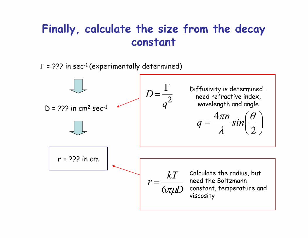
r = ??? in cm
3 = ??? in sec-1 (experimentally determined)
D = ??? in cm2 sec-1
Finally, calculate the size from the decay constant
DkTr626
)
2qD 3)
789
:;<)
24 =.6 sinnq
Diffusivity is determined… need refractive index, wavelength and angle
Calculate the radius, but need the Boltzmannconstant, temperature and viscosity

What is left?Need a systematic way to determine 3’s
Monomodal Distribution
Non-Monomodal Distribution
Linear Fit
Exponential Sampling
CONTIN regularization
Cumulant Expansion
the distribution of particle sizes defines the approach to fitting the decay constant

What is left?Need a systematic way to determine 3’s
Monomodal Distribution
Non-Monomodal Distribution
Linear Fit
Exponential Sampling
CONTIN regularization
Cumulant Expansion
First, consider the monomodal distribution, where the particles have an average mean with a distribution about the mean (red box, first)

Tau
0 1000 2000 3000 4000 5000
C(! )
1e-4
1e-3
1e-2
1e-1
Tau
0 1000 2000 3000 4000 5000
C(! )
0.0
0.2
0.4
0.6
0.8
!*! DqlnB
B)(Gln 22 20)789
:;< 0
Simplest- the ‘basic’ linear fit
Take the logarithm of the normalized correlation function
ln *
Slope = -2Dq2
C(!)
Assumes that all the particles fall about a relatively tight mean
ln C(!)
Long ! there is just noise…
… but, need Long ! for a good B

Cumulant expansion
+ , + ,1 33)A 30
01 deGg !!
+ , )q(S)q(PMG 2)3
+ , solid : )( 6RRNG /3
+ , (vesicle) shell hollow : )( 4RRNG /3
Integral sum of decay curves
Probability Density Function(Coefficients of Expansion)
Intraparticle Form FactorAnd Interparticle Form Factor
that both DEPEND ON q
Larger particles are ‘seen’ more…
Assumes that the particles distribution is centered on a mean, with a Gaussian-like distribution about the mean.
Where to start…

Then, re-arrange the Seigert Relationship in terms of a cumulant expansion
Recall that the correlation function can be expressed as
+ , + , + ,!*!! 12 2 glnlnB
BGlncln 0)"#$
%&' 0
)
Cumulant expansion is a rigorous defined tool of re-writing a sum of exponential decay functions as a power series expansion… so, that the sum from the previous page is replaced by the expansion (GET BACK HERE IN A FEW MINUTES)
+ , + , + ,1)@BAA
) 001 !!!! d
!nik
!nikgln
nn
n
nn
http://mathworld.wolfram.com/cumulant.html
+ , + ,1 33)A 3
01 dPeg i !!

… need to carry through some mathematics
+ , + ,!!! 303030) eeg1
First, define a mean value
is the mean ‘gamma’3
+ , + , + , + , + ,1 3
""#
$
%%&
'0
303(30303)1 33)
A 30A 30
0
2
01 2
1 d...!
eGdeGg !!! !!
...!x
!xxe x (0(0/0
321
32Note: power series expansion
Second, substitute the power series for the difference term (second term)

Cumulant Expansion (more)
Working through the integrals…
+ , 778
9::;
<(0(0) 30 ...
!k
!keg 3
332
22
1 3201 !!! !
Such that k2 is the second moment, k3 is the third moment, …
+ ,+ , 33031 3)A
dGk 2
02
+ , + , + , + , + ,1 3
""#
$
%%&
'0
303(30303)1 33)
A30A 30
0
2
01 2
1 d...!
GedeGg !!! !!
+ ,+ , 33031 3)A
dGk 3
03

...xx)xln( (0/( 2211Note: power series expansion
+ ,""#
$
%%&
'778
9::;
<(0(()"#
$%&' 0 30 ...
!k
!kelnln
BBGln 3
332
222
321
21
21 !!*! !
blnaln)abln( ()Note: ln of products
a b x
Note that x terms >> x2 terms, so that x2 are negligible
Cumulant Expansion (even more)

+ , ...KlnB
BGln 0(30)"#$
%&' 0 22
22 2 !!*!
Cumulant Expansion (more…)
average decayintercept polydispersity
Polydispersity index 223
)kC
… and indicates the width of the distribution
005.0)C is mono-dispersed
Note:Multiplied
by 2

Sample of Cumulant Expansion390 nm Beads
+ ,!30*)"#
$%&' 0! 2ln
BBGln 2linear
+ , 222
2 K2lnB
BGln !(!30*)"#$
%&' 0!
quadratic
+ , 33
3222
23
KK2lnB
BGln !0!(!30*)"#$
%&' 0!cubic
quartic + , 44
433
3222
212K
3KK2ln
BBGln !(!0!(!30*)"#$
%&' 0!
Gamma
~ Poly
~ Skew
~ Kurtosis

Examine residuals to the fit
uncorrelated
correlated

What is left?Need a systematic way to determine 3’s
Monomodal Distribution
Non-Monomodal Distribution
Linear Fit
Exponential Sampling
CONTIN regularization
Cumulant Expansion
Second, consider the different non-monomodal distribution, where the particles have a distribution no longer centered about the mean (red box, next)
Multiple modes because of polydispersity, internal modes, interactions… all of what make the sample interesting!

Exponential Sampling for Bimodal Distribution
+ , !! ieag i30@)1
To be reliable the sizes must be ~5X different
e.g. bimodal distribution
Assume a finite number of particles, each with their own decay

Pitfalls• Correlation functions need to be measured properly
a) Good measurements with appropriate delay times
b) Incomplete, missing the early (fast) decays
c) Incomplete, missing the long time (slow) decays

CONTIN Fit for Random Distribution
+ , + ,D E + ,dttfetfLsF st1))A 0
0
Laplace Transform of f(t)
In light scattering regime.
+ , + ,D E + , 31 3)3)A 30 dGeGLg0
1!!
size distribution function
So, to find the distribution function, apply the inverse transformation which is done by numerical methods, with a combination of minimization of variance and regularization (smoothing).
+ , + ,D E!11 gLG 0)3
+ , + ,D E + ,dttfetfG ti1A
A0
F0)G)F
Note: Fourier Transform

CONTIN• Developed by Steve Provencher in 1980’s
• Recognize that
is an example of a “Fredholm Integral” where
This is a classic ill-posed problem – which means that in the presence of noise many DIFFERENT sets of A(s) exist that satisfy the equation
+ , + ,D E + , 31 3)3)A 30 dGeGLg0
1!!
1) dssAsrKrF )(),()(
measured object of desire defines experiment

CONTIN (cont.)
So how to proceed?1. Limit information – i.e., be satisfied with the mean
value (like in the cumulant analysis)2. Use a priori information
– Non-negative G($) (negative values are not physical)– Assume a form for G($) (like exponential sampling)– Assume a shape
3. Parsimony or regularization– Take the smoothest or simplest solution– Regularization (CONTIN)
ERROR = (error of fit) +function of smoothness (usually minimization of second derivative)
– Maximum entropy methods (+ p log (p) terms)

Analysis of Decay Times
+ , + ,!! rDDqeg 61
200/3
q2
Slope = Dapp
Diffusion (translation)Finite Rotational Diffusion
3
q2
Slope = Dapp
Dr
Rotational diffusion can change the offset of the decay – can also observe withdepolarized light
First question: How do decay times vary with q?
$= Dappq2 where Dapp is a collective diffusion coefficientthat depends on interactionsand concentration

fkTD ) Shape factor: A hydrodynamic term
that depends on shape
Cylinders
+ ,
+ ,+ ,
7777
8
9
::::
;
<"#$
%&' 0(
"#$
%&' 0
)
abab
ab
ab
f2/12
3/2
2/12
11ln
1Prolate
b
a
Worms
+ ,21 231 DDD ()
D1
D1
+ ,L
KTDLlnD
o6H3)
Not spheres… but still dilute, so D = kT/f

Concentration Dependence• In more concentrated dispersions (and can only find
the definition of ‘concentrated’ generally by experiment’), measure a proper Dapp, but because of interactions Dapp (c)
• Again, D = <thermo>/<fluid> =kT(1 + f(B) + …)/fo(1 + kfc + …)
So Dapp= D0 (1 + kDc + …)
with kD = 2B –kf – %2
like a second virial coefficientfor diffusion
partial molar volume of solute (polymer ormicellar colloid)

Virial Coefficient• Driving force =
1
1
(/
0()778
9::;
<IJI 0
...]1)r-(g(r)4-kT[1
density lowat
]1)((41[
2
12
dr
rgdrrkTT
6K
6KK
1 00)
((/778
9::;
<IJI
drrrg
BkTT
22
2
)1)((4B
where
...]1[
density lowfor so
6
KK

Multiple Scattering
single scattering multiple scattering
•Three approaches
• Experimentally thin the sample or reduce contrast• Correct for the effects experimentally• Exploit it!

Diffusing Wave Spectroscopy (DWS)• In an intensely scattering solution, the light is
scattered so many times the progress of the light is essentially a random walk or diffusive process
• Measure in transmission or backscattering mode
• Probes faster times than QLS
• See Pine et al. J. Phys. France 51 (1990) 2101-2127

SummaryOriented particles create interference patterns, each bright spot being a speckle. The speckle pattern moves as the particle move, creating flickering.
All the motions and measurements are described by correlations functions• G2(!)- intensity correlation function describes particle motion• G1(!)- electric field correlation function describes measured fluctuationsWhich are related to connect the measurement and motion
Analysis Techniques:• Treatment for monomodal distributions: linear and cumulant fits• Treatment for non-monomodal distributions: Contin fits• Interactions, polydispersity, require careful modeling to interpret
Other motions, such as rotation, can be measured
"#$
%&' ()
22 11 )(gB)(G !*!