www.eprg.group.cam.ac.uk

EP

RG

WO

RK

ING

PA

PE

R

Abstract

Dynamic Long-Term Modelling of Generation Capacity Investment and Capacity Margins: a GB Market Case Study

EPRG Working Paper 1201 CWPE Working Paper 1217

Dan Eager, Benjamin Hobbs and Janusz Bialek

Many governments who preside over liberalised energy markets are developing policies aimed at promoting investment in renewable generation whilst maintaining the level of security of supply customers have come to expect. Of particular interest is the mix and amount of generation investment over time in response to policies promoting high penetrations of variable output renewable power such as wind.

Modelling the dynamics of merchant generation investment in market environments can inform the debate. Such models need improved methods to calculate expected output, costs and revenue of thermal generation subject to varying load and random independent thermal outages in a power system with high penetrations of wind.

This paper presents a dynamic simulation model of the aggregated Great Britain (GB) generation investment market. The short-term energy market is simulated using probabilistic production costing based on the Mix of Normals distribution technique with a residual load calculation (load net of wind output). Price mark-ups due to market power are accounted for. These models are embedded in a dynamic model in which generation companies use a Value at Risk (VaR) criterion for investment decisions. An `energy-only' market setting is used to estimate the economic profitability of investments and forecast the evolution of

www.eprg.group.cam.ac.uk

EP

RG

WO

RK

ING

PA

PE

R

security of supply. Simulated results for the GB market case study show a pattern of increased relative security of supply risk during the 2020s. In addition, fixed cost recovery for many new investments can only occur during years in which more frequent supply shortages push energy prices higher. A sensitivity analyses on a number of key model assumptions provides insight into factors affecting the simulated timing and level of generation investment. This is achieved by considering the relative change in simulated levels of security of supply risk metric such as de-rated capacity margins and expected energy unserved.

The model can be used as a decision support tool in policy design, in particular how to address the increased `energy-only' market revenue risk facing thermal generation, particularly peaking units, that rely on a small number of high price periods to recover fixed costs and make adequate returns on investment.

Keywords Power generation economics, Mix of Normals distribution, Thermal power generation, Wind power generation.

JEL Classification O13, P4, Q4

Contact d.eager@ed.ac.uk Publication January, 2012 Financial Support UKERC NERC NE/C513169/1, Supergen Flexnet

program, U.S. NSF EFRI Grant 35879

1

Dynamic Long-Term Modelling of Generation

Capacity Investment and Capacity Margins: a

GB Market Case Study

D. Eager, B. F. Hobbs, and J. W. Bialek

Abstract

Many governments who preside over liberalised energy markets are developing policies aimed

at promoting investment in renewable generation whilst maintaining the level of security of supply

customers have come to expect. Of particular interest is themix and amount of generation investment

over time in response to policies promoting high penetrations of variable output renewable power such

as wind.

Modelling the dynamics of merchant generation investment in market environments can inform the

debate. Such models need improved methods to calculate expected output, costs and revenue of thermal

generation subject to varying load and random independent thermal outages in a power system with

high penetrations of wind.

This paper presents a dynamic simulation model of the aggregated Great Britain (GB) generation

investment market. The short-term energy market is simulated using probabilistic production costing

based on the Mix of Normals distribution technique with a residual load calculation (load net of wind

output). Price mark-ups due to market power are accounted for. These models are embedded in a dynamic

model in which generation companies use a Value at Risk (VaR)criterion for investment decisions. An

‘energy-only’ market setting is used to estimate the economic profitability of investments and forecast

the evolution of security of supply. Simulated results for the GB market case study show a pattern of

increased relative security of supply risk during the 2020s. In addition, fixed cost recovery for many new

D. Eager is with the Institute for Energy Systems, The University of Edinburgh, EH9 3JL, UK, d.eager@ed.ac.uk

B. F. Hobbs is with the Department of Geography and Environmental Engineering, Johns Hopkins University, Baltimore,

Maryland 21218, USA, bhobbs@jhu.edu.

J. W. Bialek is with the Energy Group, School of Engineering, The University of Durham, DH1 3LE, UK.

Janusz.Bialek@durham.ac.uk

2

investments can only occur during years in which more frequent supply shortages push energy prices

higher. A sensitivity analyses on a number of key model assumptions provides insight into factors

affecting the simulated timing and level of generation investment. This is achieved by considering the

relative change in simulated levels of security of supply risk metric such as de-rated capacity margins

and expected energy unserved. These results provide insights into the increased ‘energy-only’ market

revenue risk facing thermal generating units, particularly peaking units that rely on a small number of

high price periods in order to recover fixed costs and make an adequate return on investment.

Index Terms

Power generation economics, Mix of Normals distribution, Thermal power generation, Wind power

generation.

I. I NTRODUCTION

When making an economic assessment of the potential for generating capacity investments,

we must model varying loads (e.g., in the form of the load duration curve), the expected

contribution of generating units to serving these loads, and the revenues they receive by doing

so. It is helpful if the technique used is computationally fast, accurate and robust, especially

when multi-year simulations of a market are to be repeatedlyrun. One approach is to use

probabilistic production costing, a long established method for calculating the expected output

and costs of a thermal generation system subject to varying load and random and independent

forced outages [1, 2]. The first focus of this paper is the integration in a dynamic capacity

investment simulation of a probabilistic production costing method that considers the annual load

curve and convolves it with generator outages using the Mix of Normals distribution (MOND)

approximation. This production costing method was first described in [3] and then extended and

used for the calculation of equilibrium capacity investment in a power market in [4] and [5],

respectively. In this study, the method is applied for the first time to a nonequilibrium setting as

part of a dynamic market simulation.

The second focus of the work is to assess the impact of high penetrations of wind power

on the investment risks associated with conventional thermal generation. Therefore the method

above is extended to include a residual load calculation (load net of wind output) using empirical

load and simulated wind data. This residual load data is thenused in the MOND production

costing model. Finally, the MOND model is incorporated in the dynamic investment model and

3

applied to a simplified GB power system for an assumed (exogenously increasing) installed wind

capacity.

The goal of this research is to address concerns about whether ‘energy-only’ markets (i.e.,

without capacity mechanisms) with high penetrations of wind are capable of inducing timely

generation investments over a long-term time frame. Examples of ‘energy-only’ markets currently

operating include GB, Australia’s National Electricity Market, Alberta, Nordpool, Ontario and

Midwest ISO. This is of particular interest to policy makerswhose combined goals are to promote

investment in renewable generation, maintain an adequate level of resources, and reduce customer

costs.

The dynamic model employs classical control theory to capture the interactions between

electricity supply and demand. It shares similarities withexisting dynamic models of merchant

generation investments (e.g., [6–9]), however this particular application to the GB market with a

high wind penetration is unique. Furthermore, the production costing methods used by previous

dynamic models are deterministic, and therefore underestimate average costs (due to Jensen’s

inequality [10]).

This paper is organised as follows: in Section II, the dynamic investment model in which

the MOND technique is embedded is described. Features of theinvestment decision element

of the model are provided in Section III. In Section IV a MOND is formally defined and

its application to a market situation is given. Section V describes input assumptions and the

wind models used. The purpose of this paper is to present and illustrate a methodology. For

the purposes of illustration, a number of assumptions are made that in an actual application

would require careful validation. Results from the dynamic simulation of capacity investment in

a system with an existing installed capacity similar to thatof GB are given in Section VI and

finally, Section VII presents conclusions.

II. T HE INVESTMENT MARKET MODEL

Techniques from control theory are used to model market investment dynamics (Fig. 1).

Because the model is dynamic, current market conditions (e.g., capacity under construction

or retirements), prices and their predictions are fed back to the investment block, modifying

the investment behaviour. The resulting investment decisions are then fed back to the pricing

mechanism, hence closing the loop.

4

Fig. 1. Modelling generation capacity investment as a control problem; investment can be viewed as a negative feedback control

mechanism with current and future energy prices (as a function of generation capacity margin) acting as a feedback signal.

The dynamics of the system concern the evolution of installed generation capacity and rate of

demand growth. The rate of change in capacity at a particulartime-step depends on new plant

coming online or being de-mothballed net of any plant being retired or mothballed. Both are

delayed signals from some earlier time. In the case of new plant, this delay is the lead time

for construction, and in the case of retiring plant, this delay is the design lifetime. Mothballing

requires zero delay, whilst de-mothballing requires a delay that is significantly less than full

construction. An aggregate approach is taken whereby capacity is combined into five technology

categories, namely nuclear, coal, wind, CCGT and OCGT, each with its own financial and

technological characteristics.

The elegant notation used in [11] is employed to formally define the state of the system. That is,

the state of the dynamic system is defined by the vectors(Ix, ψx) whereψx = {(ηj, ξj), i = 1 . . . nx}and−τx < η1 < η2 < . . . < ηnx

. The ordering convention ensures that the oldest investment

block ξ1 will be completed first at timeη1 + τx [11]. Note thatηj indicates the time at which

the decision is taken, andnx is the number of projects of typex under construction.Ix is the

installed capacity of plant typex, andτx is the expected build time. The indexj provides the

total number of non zero investment years since time zero. The control system is now defined

5

as the volume of installed capacityI(t), which is a parallel cascade of the four technology

categories. Each single category is defined by a Delay Differential Equation (DDE):

dIxdt

=∑

(ηj ,ξj)∈ψx

ξjδ(t− ηj − τx) −∑

(ηj ,ξj)∈ψx

ξjδ(t− ηj − τx − αx), (1)

whereδ(t) is the Dirac delta function. The first term in (1) accounts forthe addition of capacity

ξj installed at timeηj + τx. The second term accounts for deletion of capacityξj built at time

ηj + τx and retired at timeηj + τx +αx, whereαx is the expected lifetime. The equation can be

extended to include mothballing or premature retirement ofcapacity with an additional variable

introduced to represent the lead time to de-mothball.1 Each lump in (1) consists of a number of

smaller components that represent individual generating units. These are 500 MW for nuclear and

coal, 200 MW for CCGT and 50 MW for OCGT. Note that any mothballed capacity continues

to age whilst it is “disconnected” from the system.

Evaluation of potential investments by generating firms is simulated by predicting future

investment revenues and costs; this prediction uses marketconditions in the “real-time” (actually,

annual) energy market simulation as initial conditions andthen predicts the future state of the

system during the lifetime of a potential investment. Crucial uncertainties such as future demand,

fuel prices and wholesale energy prices are all simulated inthe prediction. The model does not

consider the transmission network and is conceptually a single bus system.

III. G ENERATION CAPACITY INVESTMENT

In order for adequate capacity to be maintained in the face ofdemand growth and retirement of

existing capacity, investment in new capacity must be forthcoming. In this model the investment

decision is taken annually and is considered an irreversible decision. It is based on the Net

Present Value (NPV) of anticipated future profits.

A. Investment model logic

Investors are assumed to have the modelling capabilities available to formulate a reasonable

approximation of the effect of wind generation on residual demand. That is, the investors are

1Note that any mothballed capacity must continue to age whilst it is “disconnected” from the system to ensure it is permanently

retired once it reaches the end of its design lifetime.

6

rational, but only within the limits of the information available to them, and thus do not possess

perfect information about the future state of the system. This design follows the adaptive

expectations hypothesis and has been applied in other dynamic models (e.g., [6, 8, 9, 12]).

Plainly boom and bust type dynamics will be less severe if investors have rational expectations

(see [13]) because they eliminate systematic forecast errors, however this is arguably not possible

in most electricity markets owing to their relative infancyand ongoing modification [14]. These

overshoot dynamics are further confounded by the limited forecasting certainty which modelling

tools can provide concerning variables such as economic growth and future weather patterns.

Note that variations in weather patterns are likely to average out to zero over the economic

lifetime of an investment and thus do not affect decisions about capacity expansion.2

For simplicity, a single investor who is well acquainted with the structure of the market

and capable of securing the necessary debt to finance large-scale plant investment is modelled.

This representative agent approach has been used by other dynamic capacity market models

(e.g., [14]). When estimating the profitability of an investment, a Monte Carlo (MC) approach is

taken to obtain a probability distribution of profitabilitywhereby estimates for conventional plant

already under construction (including delays), demand growth, and fuel prices are considered

stochastic.

The representative agent is aware of conventional plant already under construction at the start

of each decision process. However there is uncertainty about a) the time remaining to build these

plants, b) whether they will in fact make it to operation, andc) if rivals will jump in and invest

in response to increases in expected profits. In the base case, generators assume all plant will

come online with 100% certainty, and remaining build time isstochastic. This is modelled as

the sum of the expected build time (minus one year) plus a random variable (r.v) that is sampled

from a lognormal distribution,lnN(µ, σ2), whereµ andσ are the mean (one year) and standard

deviation (six months) of the distribution, respectively.Decision making under uncertainty is

modelled by taking a risk averse attitude to investment; this is discussed in the next sub-section.

Currently operational plant is expected to generate for the duration of its design lifetime.

Fuel and carbon forward prices are based upon the UK Department of Energy and Climate

Change (DECC) central case estimates [15, 16]. Assuming investor price forecasts are similar to

2Under the heroic assumption that climate change does not impact on future weather.

7

these estimates,3 the investor model uses the DECC estimate plus a r.v. to estimate future fuel

prices. This r.v. is modelled as a mean reverting stochasticprocess with seasonality [18]:

dFt = α(m(t) − Ft)dt+ v(Ft)dWt, (2)

m(t) =1

α

dq

dt+ q(t), (3)

whereFt is the price at timet, q(t) is the DECC estimate,m(t) is the time dependent mean

reverting level which depends on the DECC estimate,v is the volatility,α is the speed of mean

reversion andW is a standard one-dimensional Brownian motion [19]. Initially, α = 0.7 in

all cases (indicating a reasonably short excursion length)and v is 5%, 7%, 10% and 20% for

uranium, coal, gas and carbon prices, respectively to reflect the relative price volatilities.

Investors consider annual load growth to be stochastic and is sampled from a Normal dis-

tribution. Our application assumes a mean of 0% and standarddeviation of 1%. This is based

on variations in demand growth [14] as well as the perceptionthat economic growth could be

offset by increased energy efficiency (e.g., [20]), thus allowing for small or even negative load

growth.

The present value of an investment in technologyx (i.e., nuclear, coal, CCGT, OCGT) at time

τx is given by:

Vx =αx∑

i=τx

GM ix − FCx

(1 + r)i−τx− (ICx +DCx) (4)

wherer = (χx) · γ + (1 − χx) · ǫx is the firm’s weighted average cost of capital (WACC), with

χx andγ as the gearing ratio and expected bond return (assumed to be 8%) respectively, andǫx

is the required investor equity return.GM ix is the gross margin (cf. (24) or (37) depending on

market bidding assumptions) for yeari, FCx is the generator fixed operating costs, andτx and

αx (cf. (1)) are both expressed in years.ICx is the present worth of the investment cost:

ICx =τx−1∑

i=0

Mxi cxpx(1 + r)−(i−τx), (5)

wherepx is the construction cost (£/MW), cx is the plant capacity,,Mxi is the capital expenditure

vector for the project with∑τx−1i=0 Mx

i = 1. For simplicity, the expenditure schedule uses a lagged

3Which in the case of natural gas match quite well with available future prices from ICE Futures Europe (out to 2017) but

are arguably a little low for coal - at the time of writing, Newcastle futures were rising at about 1.5% annually not falling by

6% as suggested by DECC [17].

8

formulation with

Mxi = zMx

i+1 (6)

wherez = 0.8 (i.e., the capital outlay increases by 25% each year). Totalinterest accumulated

during construction is given byTIACx = ICx − cxpx. Finally, DCx is the present worth

of the decommissioning cost. Only nuclear projects have considerable decommissioning costs

(estimated at 12% ofpx4); in the case of other plant types the decommissioning liabilities are

assumed to be offset by the salvage value of the assets [22]. Nuclear decommissioning is assumed

to take 150 years and the equivalent incidence of capital outlay matrix contains 0.05 for the first

10 entries and (i.e., 50% of total decommissioning coming infirst 10 years after closure) and

the remaining entries are1/140 (i.e., 50% of cost spread over 140 years).

All cashflows are discounted to the start of the first year of operation. The total annualised

costs per unforced MW (TAFC) (£/unfor.MW/yr) are given by:

TAFCx =Acrfx (ICx +DCx) + FCx

1 − ρx, (7)

whereAcrfx is the deferred capital recovery factor andρx is the generator FOR.

Only the firstn years of expected revenues are stochastically simulated bythe investor (here

n = 7); for the remaining years the (discounted) average of the simulated revenues are used

(e.g., similar to [14]), i.e., assume that simulated pricesfor the first 7 years of plant operation are

representative of the total expected plant lifetime. Furthermore, investors cap the total expected

annual revenues received from scarcity rents (see Section IV-C) at the annualised cost of an

OCGT. These actions ensure that expectations about future revenues are not unduly influenced

by high forward simulated wholesale prices owing to generation retirements far in the future.

No regulatory price caps are implemented in the real-time simulation.

Investors in peaking capacity (i.e., OCGT) assume an additional revenue of£10,000/unforced

MW/yr can be obtained from the ancillary services (AS) market. AS revenues form a critical

component of peaking capacity profitability, however they are insufficient by themselves to trigger

investment and a combination of energy market and AS revenueis required in order to obtain

adequate gross margins. Investors will not include AS revenues in the profitability calculation

if OCGT capacity exceeds 8 GW (i.e., volume of installed OCGT capacity at the start of the

4Estimated to be between 9-12% by the World Nuclear Association [21].

9

simulation, c.f. Table III), this essentially limits the total obtainable revenue from AS if the

volume of peaking capacity becomes large. However, in account of the point made above, this

limit should not unduly dampen peaking capacity investment.

Because the model randomly samples capacity construction times, fuel prices and load growth,

a large sample is required in order for investors to obtain reliable estimate of expected project

value (4). Here, 100 MC simulation runs are carried out for each plant type in each decision

year.

B. VaR criterion

Value at Risk (VaR) is a common criterion used in finance when investors place a high priority

on avoiding poor outcomes (i.e., they are risk averse) [23].Generally speaking, given a project

valueV , and defining the level of risk aversion byq, the VaR is defined as the valuevq such

that p(V ≤ vq) = 1 − q.

In this model, the distribution of potential profits are constructed from the MC simulations

of the stochastic variables and a risk averse investor withq = 5% is assumed. The distribution

of Vx in (4) is computed by MC simulation for each plant type and an investment is deemed

attractive ifp(Vx > V optx ) ≥ (100 − q)%, whereV opt

x is the minimal acceptableVx; i.e., V optx is

a lower bound for the project value used in the VaR criterion.This is assumed to be zero (i.e.,

investors recover initial investment and receive adequatereturn on investment in account of the

WACC applied in (4)).

The decision to mothball (or de-mothball), is based on the predicted gross margins over fixed

operational costs (AGM) (£/MW) for the next three years of operation averaged over the MC

simulation runs, i.e.,

AGMx =1

100

100∑

j=1

3∑

∀j,i=1

GM ix − FCx

(1 + r)i. (8)

If this is negative (or positive) then some currently operational (or offline) plant will be moth-

balled (or de-mothballed).

C. Modelling aggregate investment response

In some circumstances the expected profitability of new investments is extremely high, thus

triggering a wave of new builds. In such cases, the investment rate will be limited by: 1) the

10

firm’s beliefs about how many other market participants willmove to invest; 2) the impact of new

investment on the profitability of their existing plant; and3) the ability of the firm to secure the

debt required to fund multiple projects [8]. Using an aggregate investor response curve is useful

in models of this type. For instance, in [14], the aggregate investment rate is increasing with

the “risk-adjusted forecast profit”, which is derived from the investor’s (risk averse, concave)

utility function. Also in [8], an S-shaped nonlinear function of Profitability Index (PI) is used

and various profitability functions are used in [7] to model investment rates based on managerial

optimism concerning economic (i.e., expected profitability) and strategic (i.e., retaining market

share) considerations.

In this paper, a function is applied to the outcome of the VaR decision rule in order to estimate

the aggregate investment response of the market. This function is increasing with the expected

profitability and is given by:

ξi = max{

0, ξmax ·(

1 − e(−β·PIqx))}

, (9)

where

PIqx =V qx

(ICx +DCx)(10)

is the Profitability Index (PI) (i.e., critical (q%) Vx divided by investment cost per unit of capacity)

and ξmax is the maximum investment per year in technologyx. ξmax and β are calibrated so

zero investment is made ifPIqx < PIoptx (with PIoptx the result of substitutingV optx into (10)),

andξi = ix volume of investment is made ifPIqx = 1, whereix is a fixed constant. Note thatξi

provides the link to the state equation (1).

The function used in the base case is shown in Fig. 2 with fixedix = 2 GW andξmax = 4 GW,

andβ = 0.7 resulting from the calibration. Changingβ alters the aggregate response, as shown

by the dotted lines. There is the potential to include different response curves within each fuel

or peak/base generator type (e.g., as in [8]). There is also an additional step whereby after each

2 GW of capacity of investment is triggered, the investor decision is re-run to ensure that no

other plant types become more attractive in relation to other options as a result of this addition.

This maintains the iterative adding characteristic in [24]whereby the decision is to 1) invest in

the most profitable technology (if any), followed by 2) a re-run of the investment decision with

all new investments accounted for. 1-2 are then repeated until no additional plants are profitable.

11

For multiple investments withPIx > 0, the option with the highestPIx is chosen. Finally, total

annual investments are limited to 10% of installed capacity.

Fig. 2. Plot of model aggregate investment response curve defined by (9) (solid line) whereix = 2 GW andξmax = 4 GW .

Also shown are the minimum investment lump sizes along with curves for different values ofβ.

The volume (GW) of plant mothballed or de-mothballed is determined simplistically using

the linear functionξi = min(M,AGMx/104), i.e., decreasing or increasing inAGMx (£/MW)

up to a maximum ofM GW (Fig. 3). In this caseM is chosen to be 2 GW.

Fig. 3. Plot of model aggregate mothballing response curve. Note that the x-axis has been rescaled to (£/kW).

12

IV. PRODUCTION COSTING BY MIX OFNORMALS

When estimating expected long-run production costs, there is a need for a reasonably accurate

approximation of the load duration curve (LDC). A MOND approximation meets this requirement

and is also very easy to convolve with plant outages for the expected output calculations.

A MOND is described as follows: consider a set,Y = {y1, . . . , yn}, of Normally distributed

r.vs. with theith element having meanµi and varianceσi. Let Φ(x|µi, σi) be the cumulative

distribution function (cdf) ofyi. A MOND is a convex combination of the Normal distributions

and is defined by

F (x) =n∑

i=1

piΦ(x|µi, σi), (11)

with∑ni=1 pi = 1 andpi ≥ 0, wherepi is the weight of the componentyi [3]. Let µ andσ be the

mean and standard deviation respectively of the cdf described by (11). These parameters have

the following properties:

µ =n∑

i=1

piµi, (12)

σ2 =n∑

i=1

pi(σ2i + µ2

i ) − µ2. (13)

Another property is that the sum of two variables each distributed as a MOND is itself a MOND.

The proof of these properties is in appendix A of [3].

The process starts by splitting the time horizon over which costs are calculated into periods.

In this case, the duration of each period is one year; although, shorter periods can also be used

to account, e.g., for seasonal capacity. The expected load at each hour is a r.v.

A MOND fit for approximating the annual LDC (MW) is required. For example, iffL(x)

is the probability density function of load andFL(x) is the cumulative distribution function of

fL(x), then the LDC is simply the rotated and rescaled loadexceedencedistribution.5 This is

the inverse of8760(1 − FL(x)) where

FL(x) =K∑

k=1

pkΦk(x|µk, σk), (14)

which is a mixture ofK Normals (Φk) with the same properties as (11). For a particularK, the

best fitting value of eachµk, σk andpk can be found by solving an optimization problem that

minimizes the sum of squares of the difference between observed and fitted values of the LDC.

5The exceedence distribution givesP (X > x), that is the probability that the r.v.X (in this case load) is greater thanx.

13

To illustrate the accuracy of this technique at approximating a LDC, Fig. 4 shows the distribu-

tion of the GB hourly loads for the period 2005-09 (normalised by the year’s average demand)

and the fitted distribution. This normalisation is necessary when comparing multiple years to

account for demand growth. The difference between the two LDC plots in Fig. 4(b) is not visible

at this scale owing to the excellent fit provided by the MOND.

(a) (b)

Fig. 4. (a) MOND pdf (4 Normal components clearly visible by their distinctpeaks) and histogram of normalised load data

and (b) LDC fit with negligible visible difference between mix of 4 Normals and empirical data.

A. MOND with conventional thermal generation (after [3])

The next step is to estimate the available capacity for a set of generating units. The available

capacity at each hour from a particular unit is a r.v. which ischaracterised by the unit’s Forced

Outage Rate (FOR). Let the capacity of unitu be defined bycu, its FOR byρu and expected

available capacityGu = cu(1 − ρu). That is, the distribution of the unit’s available capacity

follows a Bernoulli distribution between zero andcu; thus, the unit is either available at full

capacity (with probability1 − ρu) or on full outage with (with probabilityρu).6

If mu units of typen share the same capacity and FOR characteristics and are subject to

independent forced outages, they can be treated as a single pseudo-unit (or generator) with a

6More general models exist to account for partial unit outages (e.g.,see [25]), however they are not considered here.

14

distribution with the following moments:

E(Gn) = µn = mucu(1 − ρu), (15)

V ar(Gn) = σ2n = muc

2uρu(1 − ρu), (16)

where each (pseudo-) generator,Gn, has capacitycn = mucu.7

Now the convolution property of the MOND is used to determinethe distribution for the ex-

pected load still to be served after each generator is dispatched (in merit order). This distribution

is called theeffective load duration curve(ELDC) facing the next generator to be dispatched

[26]. If the units can be grouped intoN (pseudo-) generators8 each with characteristics (15) and

(16), then we can define

Ln(x) = P

{

L−n∑

i=1

Gi > x

}

(17)

as the load minus the available capacity of generator types1 . . . n (1 ≤ n ≤ N ) [3]. If Fn(x) =

1 − Ln(x) is the cumulative probability of effective loadx = L−∑ni=1Gi facing the(n+ 1)th

generator, then

Fn(x) =∫ cn

0Fn−1(x+ y)fn(y)dy (18)

and

Ln(x) = 1 − Fn(x), (19)

wherefn(y) is the pdf of the Normal that approximates the Binomial distribution describing the

available capacity of thenth type of generation with installed capacitycn.9 Fn(x) is computed

by performing the convolution of the Normal distributions for load (which is a MOND) and

available capacity.

The convolution property of a MOND [3] is applied, with generator loading carried out by

merit order. The expected energy serveden (in MWh/yr) by generator typen can then be given

7To simplify the presentation for the remainder of the paper, the conventionwill be to use ‘generator’ when referring to a

‘pseudo-unit’ (collection of units of a given type), andcn when referring to the capacity of that generator, because this is the

last time individual units will be discussed.

8The more units in a group, the closer the Binomial distribution is to Normal.

9Technically for a Normal distribution, the bounds in (18) should be−∞ to ∞, but it is assumed here that the probability

of falling outside the physically possible range[0, cn] is negligible owing to the Binomial distribution being rescaled to 0/cu.

15

by

E[en] = 8760∫

∞

0[Ln−1(x) − Ln(x)]dx, (20)

whereLn−1(x) is the load still to be met after adding generator typen−1 andLn(x) is the load

still to be met after adding generatorn, which at the start of the convolution process (n = 0) is

obtained from (14).

The distribution for the ELDC after convolving inn generators is given by:

Ln(x) = 1 −K∑

k=1

pkΦk(x|µLk−

n∑

i=1

µGi,

[

σ2Lk

+n∑

i=1

σ2Gi

]1

2

). (21)

Thus, the ELDC is described by a MOND with the same number of component Normals as the

original LDC. An example of the iterative convolution process is shown in Fig. 5. The diagram

depicts how the remaining expected load to be served is reduced each time a group of generators

is convolved with the ELDC.

Fig. 5. Example of the convolution process. Shaded region is the expected energy served by the first unit dispatched (i.e., the

result of (20) withn = 1).

Given eachLn(x) (n = 1 . . . N ), the probability that generatorn or higher (in the merit order)

is the marginal source of energy (and so sets the price) is given byLn(0), i.e., the point where

the function crosses the vertical axis in Fig. 5. Further,

hn = Ln−1(0) − Ln(0) (22)

16

is the probability that generatorn is on the margin. This result is used in Section IV-C to calculate

expected revenues per MW for a generator belonging to this generator type in an ‘energy-only’

market setting.

The unserved energy (MW) is then simply any positive remaining load once allN generators

have been added. The annual expected energy unserved (EEU) can be calculated by integrating

LN+1(x) (i.e., after convolving in the complete set ofN generators) from 0 to∞ and multiplying

by 8760 hrs/yr. Furthermore the Loss-of-Load Expectation (LOLE) for the period is determined

by computing8760 · LN+1(0) [25].

B. MOND with a thermal-wind system

Unlike conventional thermal generation units whose individual availabilities are assumed to

be independent, wind generators rely on the availability ofthe “fuel” resource and therefore a

dependency between available wind generation at differentwind plants is introduced. As a result,

the convolution technique used to model thermal generationin [3] cannot be directly used to

account for wind power generation.

To address this issue, an exogenous wind capacity is assumedand the resulting residual LDC

facing thermal generation is computed and the MOND approximation is applied to this wind-

adjusted data set. The residual load is simply the load minusthe output from all wind plants at

each hour. By taking this approach, the analysis can take intoaccount both spatial correlations

and seasonal (e.g., monthly and diurnal) trends in wind availability and their relationship with

demand.

It is important to note that the residual LDC approach removes the chronological issues that

arise in the wind and load time series. This is particularly important in the presence of large

amounts of hydro and pumped hydro generation where chronological production costing methods

may be preferred to load duration curve methods. However this implementation of the MOND

technique is applied to the GB power system where the amount of hydro and pumped hydro

is relatively small (about 4% of capacity), so the use of a load duration curve approach is

reasonable.10

10Note that there is little scope for new build of hydro technologies in GB due to thelack of suitable sites.

17

C. Expected revenues from the energy market

In the absence of market power and unless there is a capacity shortage, the market price for

energy will equal the marginal cost of the last generator to be dispatched. If there is a capacity

shortage, and assuming there is no price cap, the price will clear at the level necessary to ration

demand to the available capacity. More precisely, because consumers are not generally exposed

to the real-time price, there is a willingness of suppliers (load serving entities in US parlance)

to pay up to the Value of Loss Load (VOLL) when there is a shortage.11 This methodology is

applied in [4] in a long-run equilibrium model; that approach is extended here to a dynamic

long run nonequilibrium setting.

During a particular year, the probability that generatorn will be at the margin is given by

(22) and the price in that event will be the marginal cost of the generator,MCn. This assumes

price-taking (competitive) behaviour by generators. Furthermore, once the convolution process

has been completed for allN generators, the probability that there will be insufficientgeneration

to meet demand is given byLN+1(0) and under this condition the price is assumed to reach

VOLL. Using the result in (22), the expected gross margin fora particular MW of capacity

belonging to generatorn when generatori is at the margin is given by (£/MWh):

Rin = max {hi(πi −MCn), 0} (23)

whereπi is the wholesale price when generatori is at the margin, which in the absence of market

power is given byMCi. Using (22) to calculate (23), the expected annual perfectly competitive

gross margin (revenue minus variable cost) used in (4) can becalculated by (£/MW/yr):

CGMn = 8760(1 − ρn)[

N∑

i=1

Rin + (hN+1(V OLL−MCn))

]

. (24)

Economists term these “scarcity rents”. It is precisely these scarcity rents that, in a simple

long-run competitive ‘energy-only’ market model, are justhigh enough to cover fixed costs and

trigger investment [27]. The main numerical work here is in computing theLn(x) in (20); once

these are known, the revenues are calculated easily by multiplying by the price - marginal cost

differentials. Note that no start-up or no-load costs are considered here.

It is assumed that in a competitive energy market, generators bid to produce electricity at

or around their marginal cost. The rules of the GB market allow for generators to trade freely,

11In a more general case, some or all customers are exposed to the real-time price.

18

i.e., there is no marginal cost bid rule in place. However this is not a problem because the

equilibrium concepts for bilateral and central pool markets have been proved equivalent (see

[28] or [29] for the Cournot case). Recent analyses of the GB market [30] showed a tendency

for balancing market (BM) prices to rise above the estimated marginal cost of the last generator

dispatched in peak demand hours. Other examples of empirical analyses which support this claim

include [31, 32]. In [31], an analysis of the Texas BM revealedevidence of bidders, particularly

smaller firms, submitting supply curves in excess of their theoretical optimal supply function.12

[32] found that a Cournot oligopoly model provided a better representation of the California,

Pennsylvania-New Jersey-Maryland (PJM) and New England wholesale markets than a perfectly

competitive model during peak hours,13 and it was during these hours that the presence of price

mark-ups was detected. This price mark-up during peak demand hours occurs because firms

can raise their bids knowing that the lack of alternative resources will mean their bids will be

accepted. In this case the market does not necessarily clearat the marginal cost of production, so

in this study price,π, includes an additional mark-up term that alters the shape of the aggregate

supply curve as the system approaches scarcity. This new price function is described in [24] and

is defined here as:

π(L,G1, G2, . . . , GN) = mc(L,G1, G2, . . . , GN) + w(L,G∗

N) (25)

wheremc(L,G1, G2, . . . , GN) is the marginal production cost of meeting the load,L, given

realised total available generationG∗N =

∑Ni=1Gi, andw(L,G∗

N) = aeb(L−G∗

N) is a function of

the capacity margin, defined as total available capacity minus load in a particular hour (similar

to [33]) whereL andG∗N are expressed in GW. Note that the parametersa andb are calibrated

so that a capacity margin of zero provides a mark-up equal to the VOLL (e.g., Fig. 7(b)).14

The use of this function can be justified by comparisons of theGB forward Market Index Price

and simulated prices with accurate fuel price data (presented in [24]), however in this example

application the parameters used vary slightly. This also agrees with the methodology used in

12Profit-maximization where profit function is based on a contract for differences between offer price and cost incurred for

supplying contractually obligated and BM quantities.

13If vertical arrangements were also accounted for in the PJM and New England case.

14For instance, for a VOLL of£10,000/MWh,a = 10, 000 andb = −1.123, and for£2,000/MWh,a = 2, 000 andb = −1.101.

19

[30] to simulate GB system marginal prices where wholesale prices were simulated using a price

mark-up function in peak hours.

For simplicity, linear variable costs are assumed for all generators, that is total variable costs

are given byCn(P ) = bnP , which leads to a stepped aggregate supply function in the short-run

(if bids are assumed to equal generator marginal cost,MCn = bn) based on the marginal costs

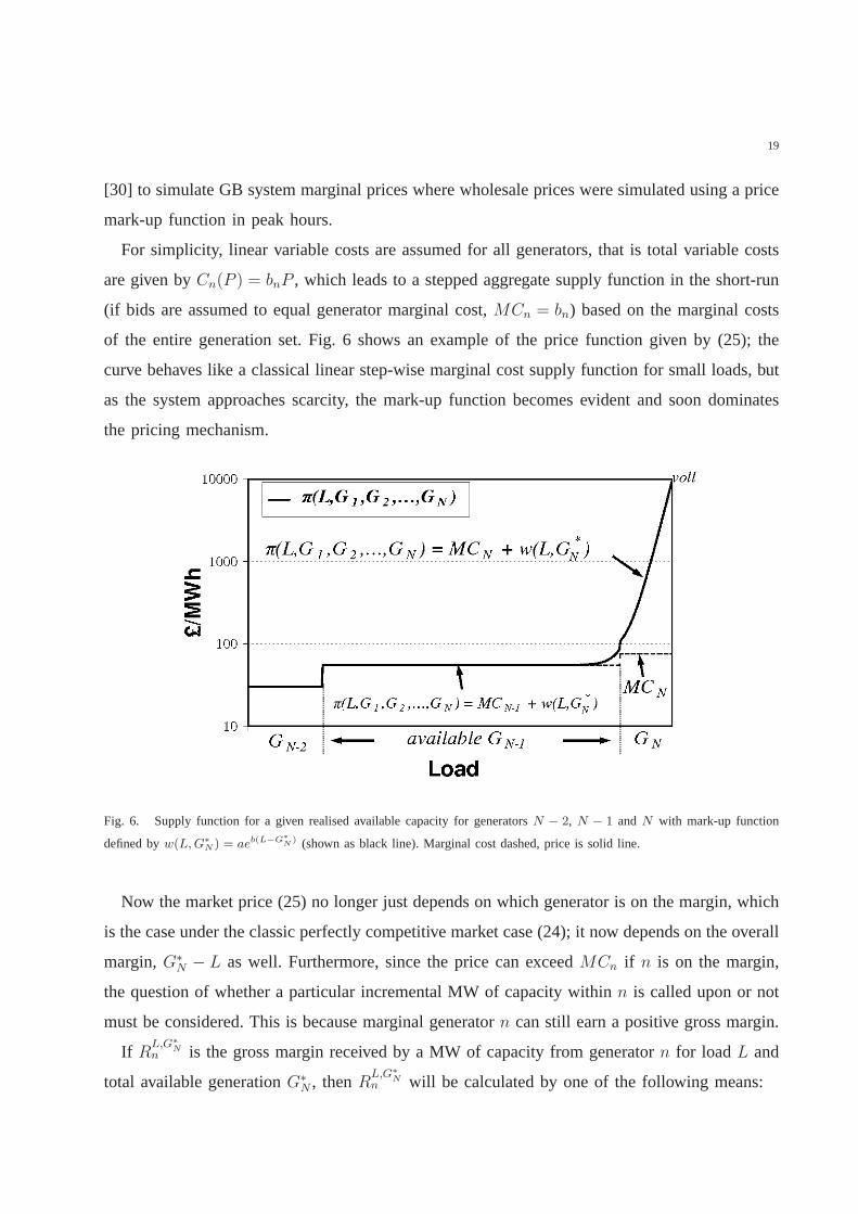
of the entire generation set. Fig. 6 shows an example of the price function given by (25); the

curve behaves like a classical linear step-wise marginal cost supply function for small loads, but

as the system approaches scarcity, the mark-up function becomes evident and soon dominates

the pricing mechanism.

Fig. 6. Supply function for a given realised available capacity for generatorsN − 2, N − 1 and N with mark-up function

defined byw(L, G∗

N ) = aeb(L−G∗

N) (shown as black line). Marginal cost dashed, price is solid line.

Now the market price (25) no longer just depends on which generator is on the margin, which

is the case under the classic perfectly competitive market case (24); it now depends on the overall

margin,G∗N − L as well. Furthermore, since the price can exceedMCn if n is on the margin,

the question of whether a particular incremental MW of capacity within n is called upon or not

must be considered. This is because marginal generatorn can still earn a positive gross margin.

If RL,G∗

Nn is the gross margin received by a MW of capacity from generator n for loadL and

total available generationG∗N , thenR

L,G∗

Nn will be calculated by one of the following means:

20

1) If the marginal generator, sayi, is belown in the merit order (i.e., has a lower marginal

cost) then the generatorn will not be dispatched andRL,G∗

Nn = 0.15

2) Else if the marginal generator has a higher marginal cost thann, then the probability of

dispatch is 1 andRL,G∗

Nn = mc(L,G1, G2, . . . , GN) + w(L,G∗

N) −MCn.

3) Else if n is the marginal generator, then the probability of dispatch isbetween 0 and 1

andRL,G∗

Nn = mc(L,G1, G2, . . . , GN) + w(L,G∗

N)pdispn −MCn

= w(L,G∗N)pdispn ,

(26)

wherepdispn is the probability that a MW belonging to generatorn is dispatched.

This probability of dispatch is approximated by

pdispn = max

(

min

{

1,−Mn−1

cn(1 − ρn)

}

, 0

)

, (27)

whereMn−1 =∑n−1i=1 Gi − L is the surplus margin afterL has been met using all available

generation lower in the merit order thann (e.g., Fig. 7). In plain terms, (27) is the ratio of the

MWs of generatorn that are dispatched to the average total MW ofn that are available (which

is will differ from the actual available MWs ofn in any particular realisation). In the event that

this margin is negative, the fractional term in (27) will be greater than 1, therefore the min{ }function is required in order to eliminate this possibility. This method of calculating dispatch

probabilities is required to account for market price mark-up (25).

The expected gross margin (24) must now be extended to consider the price function (25) and

merit order operation. This is less straight-forward than under marginal cost-based pricing (23)

because the market price mark-up requires consideration ofthe total (generation-load) margin,

MN , as well as the marginal unit.

By assuming that price mark-up is non-zero (i.e.,w(L,G∗N) > 0) only when generatorN or

N−1 is on the margin, calculation of the probability distribution ofw(L,G∗N) can be achieved by

considering the joint probability distribution of just thecapacity marginsMN−1 andMN . This

assumption is reasonable in an aggregated capacity model where the generator size is large.

What’s more, empirical evidence from the GB market (e.g., [30]) is that mark-up tends to occur

15Thus we are assuming for simplicity that dispatch is still in merit order, despite the presence of market power. However,

in oligopolies with asymmetric generating companies, a small high cost generator might produce power before a large low cost

generator, as the latter is more likely to withhold capacity. This possibility is not considered here.

21

(a) (b)

Fig. 7. (a) Aggregate supply curve showing price (solid upper line) forload L and revenue for generator of typeN − 1.

mark-up function also shown (dashed line). (b) Shows price mark-upfor different values of capacity margin and calibrations

for a = 10, 000, 2, 000 and1, 000.

predominately during peak periods when surplus margins arerelatively small, and the surplus of

available resource in other periods means the presence of market power is unlikely. Therefore, it

is reasonable to assume that price mark-up is significant only when peaking plantsN or N − 1

are on the margin.

D. Expected price mark-up calculation

Firstly, for each component of the MOND (11), we consider thejoint distribution of capacity

marginsMN−1 andMN , which is given byf(MN−1,MN). The correlation is calculated as:

corr(MN ,MN−1) = cov(MN ,MN−1)σMN−1

σMN

=σ2

MN−1

σMN−1·σMN

=σMN−1

σMN

.

(28)

22

This can be proved by considering the correlation betweenX + Y andX, whereX andY are

independent variables, then

corr(X + Y,X) = cov(X+Y,Y )√V ar(X+Y )·V ar(X)

= E(([X+Y ]−[E(X)+E(Y )])·(X−E(X)))sqrtV ar(X+Y )·V ar(X)

= E(([X−E(X)]+[Y−E(Y )])·(X−E(X)))√V ar(X+Y )·V ar(X)

= E([X−E(X)]·(X−E(X))+[Y−E(Y )]·(X−E(X))√V ar(X+Y )·V ar(X)

= V ar(X)+0√V ar(X+Y )·V ar(X)

=√

V ar(X)V ar(X+Y )

.

(29)

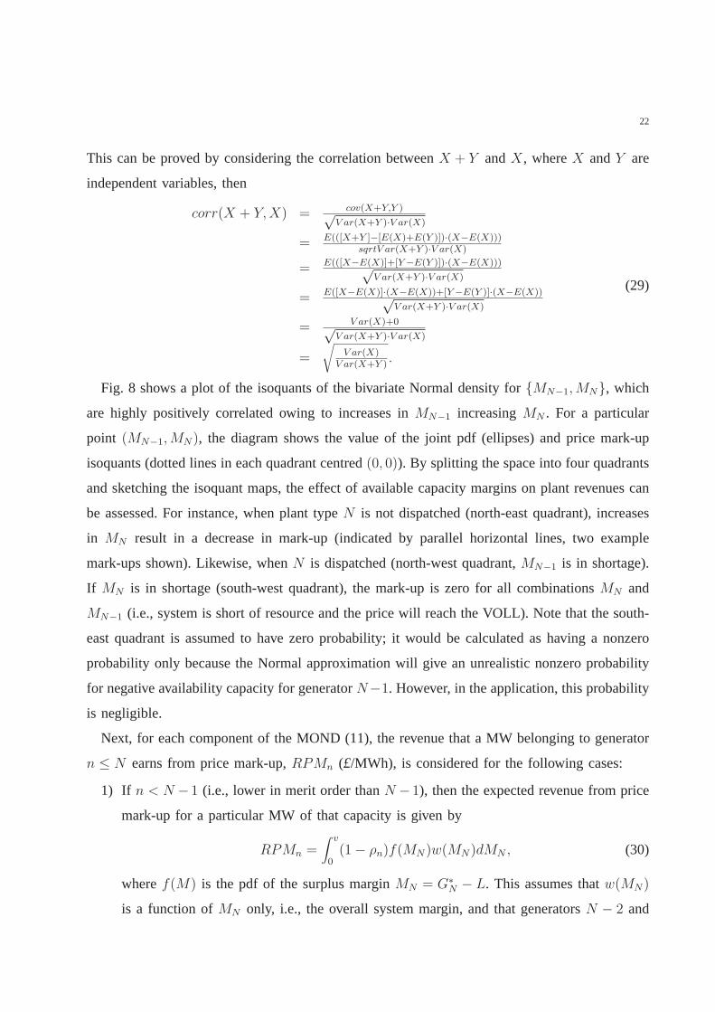
Fig. 8 shows a plot of the isoquants of the bivariate Normal density for {MN−1,MN}, which

are highly positively correlated owing to increases inMN−1 increasingMN . For a particular

point (MN−1,MN), the diagram shows the value of the joint pdf (ellipses) and price mark-up

isoquants (dotted lines in each quadrant centred(0, 0)). By splitting the space into four quadrants

and sketching the isoquant maps, the effect of available capacity margins on plant revenues can

be assessed. For instance, when plant typeN is not dispatched (north-east quadrant), increases

in MN result in a decrease in mark-up (indicated by parallel horizontal lines, two example

mark-ups shown). Likewise, whenN is dispatched (north-west quadrant,MN−1 is in shortage).

If MN is in shortage (south-west quadrant), the mark-up is zero for all combinationsMN and

MN−1 (i.e., system is short of resource and the price will reach the VOLL). Note that the south-

east quadrant is assumed to have zero probability; it would be calculated as having a nonzero

probability only because the Normal approximation will give an unrealistic nonzero probability

for negative availability capacity for generatorN−1. However, in the application, this probability

is negligible.

Next, for each component of the MOND (11), the revenue that a MW belonging to generator

n ≤ N earns from price mark-up,RPMn (£/MWh), is considered for the following cases:

1) If n < N − 1 (i.e., lower in merit order thanN − 1), then the expected revenue from price

mark-up for a particular MW of that capacity is given by

RPMn =∫ v

0(1 − ρn)f(MN)w(MN)dMN , (30)

wheref(M) is the pdf of the surplus marginMN = G∗N − L. This assumes thatw(MN)

is a function ofMN only, i.e., the overall system margin, and that generatorsN − 2 and

23

Fig. 8. Diagram showing 3-D plot of bivariate Normal of{MN−1, MN} (right) and its image on a 2-D plane (left) with

isoquant maps for the pricemarkupelement of (25).

N − 3, etc are all fully dispatched when mark-up is nonzero. The integral lower bound

in (30) is zero due to price mark-up being zero ifMN < 0. More precisely, if the overall

margin is negative then there is no mark-up and the price is set by the marginal cost of

demand (i.e., VOLL). The integral upper bound in (30) is somevalue,v, above which the

price mark-up is negligible owing to the large surplus margin (e.g., 7 GW in Fig. 7(b)).

2) Else if n = N − 1, thenRPMn is broken down into two sub-cases:

a) If MN−1 ≤ 0 (i.e., north- or south-west quadrant of Fig. 8) then

RPMn =∫ 0

−∞

∫ v

0(1 − ρn)f(MN ,MN−1)w(MN)dMNdMN−1, (31)

which is the case where all of generatorN−1’s available capacity will be dispatched

because load exceeds the available capacity of generators 1throughN − 1. Again,

the inner integral lower bound is0 becauseMN ≤ 0 results in zero price mark-up

(south-west quadrant of Fig. 8).

24

b) Else ifMN−1 > 0 (which impliesMN > 0, so north-east quadrant of Fig. 8)16 then

RPMn =∫ v

0

∫ v

MN−1

pdispN−1f(MN ,MN−1)w(MN)dMNdMN−1, (32)

wherepdispN−1 is the probability of dispatch of generatorN − 1, given by:

pdispN−1 =(1 − ρN−1)MN−2

−1 · (MN−1 −MN−2)(33)

whereMN−2 is the surplus margin after all available generation lower in the merit

order thanN − 1 has been dispatched.17 MN−2 is a r.v. and computation of its pdf is

awkward; however it can be approximated as follows:MN−2 ≈ (E(GN−1)−MN−1).

This is achieved by approximating the realised value ofGN−1 by its expectation,

(15): E(GN−1) = cN−1(1 − ρN−1).18 Leading to:

pdispN−1 ≈(1 − ρN−1)(cN−1(1 − ρN−1) −MN−1)

−1 · (MN−1 − (cN−1(1 − ρN−1) −MN−1)), (34)

i.e., the expected surplus margin over generatorn’s expected available capacity. Note

thatMN−1 > 0, soMN−2 < 0,19 and thus0 < pdispN−1 < 1.

3) Elsen = N andMN−1 < 0 andMN > 0 (i.e., north-west quadrant of Fig. 8):20

RPMn =∫ 0

−∞

∫ v

0pdispN f(MN ,MN−1)w(MN)dMNdMN−1, (35)

where

pdispN =(1 − ρN)MN−1

−1 · (MN −MN−1), (36)

i.e., the case whereMN−1 is in shortage and some volume of capacity from generatorn

(= N ) will be required to meetL.21

16We assume that the probability of being in the south-east quadrant of Fig.8 is zero because of the discussion above.

17The −1 scalar is applied to the denominator of (33) in account ofMN−2 being negative. If it was positive, thenGN−1

would not be dispatched (i.e.,pdisp

N−1 = 0), which is not considered in (32).

18Note here thatcN−1 is the capacity of the generator typeN − 1, which is the sum of a number of individual units who

share the same capacity and FOR characteristics (see footnote 7).

19In general,MN−2 could be positive, however the assumption here is that it is negative whenprice mark-up is greater than

zero.

20There is no second case here; only the case whereMN−1 < 0 is of interest (ifMN−1 > 0 thenGN is not dispatched and

mark-up revenue is zero).

21The pdf of capacity margin is Normal in account of both available generation and load (in fact, a MOND) being Normal.

ThereforeMN−1 andMN could conceivably be−∞. However, practically speaking the outer integral lower bound in (31) and

(35) is set to−1 · [maximum value of load] (i.e., the highly unlikely situation when all generation is unavailable).

25

Finally, by integrating over the subregions of the{MN−1,MN} space in Fig. 8 (i.e., using

cases 1-3 above), the expected annual gross margin for generator n can be calculated as

GMn = CGMn + E[en] ·RPMn. (37)

This is repeated for each component of the MOND.

This is an important extension to (24); by exploiting the properties of the probability distri-

bution of capacity margins, this allows for the additional revenue received from market price

mark-up to be calculated during the production costing process. Procedures for calculating price

mark-ups in probabilistic production costing models have been proposed (e.g., see [34] where a

Cournot model is proposed). To our knowledge this is the first time these derivations have been

presented.

To speed up the computation of (31)-(35), the outer integralis carried out using Gaussian

quadrature (GQ), which requires fewer function evaluations than other methods, such as the

recursive adaptive Simpson quadrature and is given by∫ 1

−1f(x)dx ≈

n∑

i=1

wif(xi) (38)

which after some manipulations, can be applied to the interval [a, b]. Heren = 100 is used.

E. Test of accuracy

To test the accuracy of this method, the results of a Monte Carlo (MC) simulation were

compared with the MOND technique. That is, for the load (a MOND) and generator cost inputs

given in Table I, capacity mix given in Table III and mark-up function calibrated to VOLL

10,000 £/MWh, random samples for load and generator availability were taken. Using these

samples, the margin,MN , price (25), and energy market gross margins were calculated for each

unit. Close attention was paid to the tail of the distributionby using importance sampling. More

precisely, high loads were oversampled using the componentNormal of the MOND with the

largest mean (i.e., row 1 in Table I) with corresponding meanµ1, standard deviationσ1, and pdf

f ∗(x). Samples were then weighted using the weighting functionW (x) = f(x)/f∗(x), where

f(x) is the 4 component MOND pdf andx is the random sample fromN(µ1, σ21).

The MC simulation was repeated106 times. The results of this test are displayed in Table II.

“MOND” shows the results for the MOND technique including the methods and approximations

26

of Section IV, above. “Monte Carlo” is for a Monte Carlo (MC) testwhere available capacity is

sampled from a Normal distribution with parameters defined by (15)-(16). Finally, “Bernoulli”

samples available capacity from a Bernoulli distribution (i.e., 0 or full capacity based on uniform

random number generation for given FORs). The Bernoulli test makes no approximations con-

cerning the distribution of available capacity or its effects on prices and mark-up, and so is the

standard against which the new MOND model should be compared. Comparing the MOND and

Bernoulli tests shows the effect of using a Normal approximation for available capacity rather

than the Bernoulli distribution. Encouragingly the MOND technique matched quite well to the

MC simulation (with only a mild over-estimation of gross margins by the MOND technique).

Further, the Normal approximation for available capacity also performs well. This test gives

confidence that the MOND approximation is a good one. Note that the “energy expected per

generator” in Table II for the Monte Carlo and Bernoulli tests is the result of multiplying the

mean utilisation across the MC runs of each generator by the total theoretical available energy

of each generator. For instance, if the capacity of generator N − 3 is 11 GW and the mean

utilisation is, say 0.75, then energy expected is given by 8760*11*0.75=72,270 GWh. For the

MOND test, this is calculated using (20).

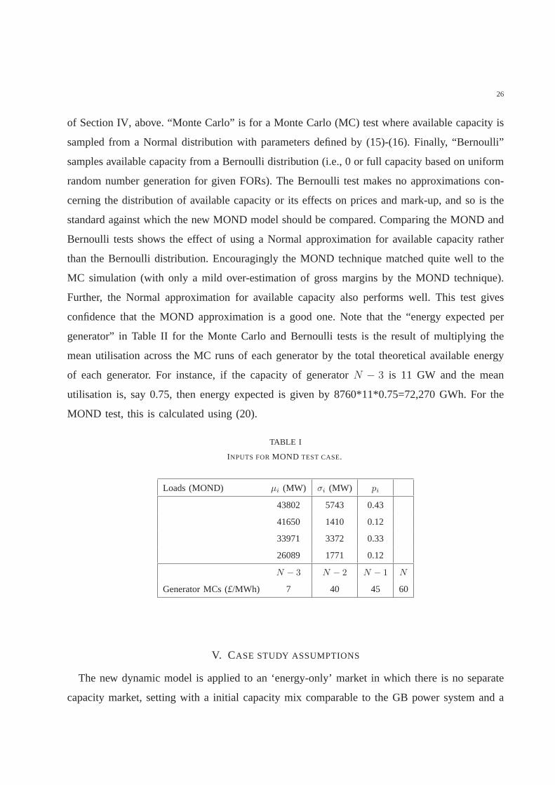
TABLE I

INPUTS FORMOND TEST CASE.

Loads (MOND) µi (MW) σi (MW) pi

43802 5743 0.43

41650 1410 0.12

33971 3372 0.33

26089 1771 0.12

N − 3 N − 2 N − 1 N

Generator MCs (£/MWh) 7 40 45 60

V. CASE STUDY ASSUMPTIONS

The new dynamic model is applied to an ‘energy-only’ market in which there is no separate

capacity market, setting with a initial capacity mix comparable to the GB power system and a

27

TABLE II

SUMMARY OF RESULTS FORMONTE CARLO TEST.

Scarcity rent (£/MWh) Price mark-up (£/MWh) Energy expected per generator (TWh)

N − 3 N − 2 N − 1 N N − 3 N − 2 N − 1 N N − 3 N − 2 N − 1 N

MOND 1.48 1.70 1.70 1.36 39.03 6.03 2.15 2.05 72.27 198.89 63.12 0.12

Monte Carlo 1.43 1.64 1.66 1.33 38.96 5.96 2.09 1.99 72.24 198.88 63.09 0.12

Bernoulli 1.41 1.61 1.63 1.30 38.91 5.92 2.04 1.94 72.24 199.40 63.11 0.12

VOLL of £10,000/MWh with a simulation time horizon of 30 years (2010-40). To reflect the

restrictions in suitable sites for nuclear builds in GB, total installed nuclear capacity is constrained

to 30 GW.

The expected hourly aggregated onshore wind output in GB is simulated using the methodol-

ogy described in [35] by obtaining GB wind speed data for 2005-09 (to match the empirical load

data), transforming to capacity factors using a Vestas V80-2 MW wind turbine power curve and

applying regional weightings derived from the current windcapacity in operation, construction,

or consented in GB.

For offshore wind, the expected hourly aggregated capacityfactors are calculated using the

simulated wind speeds from the Weather Research Forecast Model developed at the University

of Edinburgh [36]. This is a fully compressible, nonhydrostatic mesoscale atmospheric 3km grid

point model similar to the Met Office Unified Model [37]. It hasbeen validated against measured

offshore wind speed data for a number of sites [38], and in theabsence of extensive measurement

data, provides credible estimates in time and space for the GB offshore wind resource. The wind

speeds are transformed to capacity factor using the same approach as [35] using the larger Vestas

V90-3 MW power curve. The weighted regional capacity factors are based on the results from

the GB 1-3 Crown Estate Round auctions [39].

The total installed wind capacity is exogenous to the model,and is expected to increase linearly

from 2010 levels up to 30 GW by 2020 with a maximum of 35 GW in 2025, after which it levels

off. We justify this approach by the fact that, to date, large-scale investment in wind capacity is

driven by political, rather than economical considerations. It is therefore assumed that policies

28

promoting investment in wind generation are successful in meeting renewables targets,22 and the

purpose of this work is to provide insights into the responseof investment in thermal generation

and subsequent levels of security of supply risk. The allocation between onshore and offshore

areas is consistent with the data in [35] and [39].

The residual load facing thermal units for a particular houris calculated by scaling the hourly

wind production by the installed capacity and subtracting it from the full load. Fig. 9 shows an

example of the impact on the 2005-09 residual load histograms as penetration of wind increases.

Each of the 30 year’s MOND residual load curves are precalculated assuming fixed underlying

demand patterns and are then scaled over time in order to match the load growth assumptions.

(a) (b)

Fig. 9. Result of increasing installed wind capacity from (a) 2 GW to (b) 20 GW on residual load histograms. Data shown is

for 2005-09. Numbers in brackets indicate volume of onshore and offshore capacity respectively.

Data on initial 2010 system capacity in Table III is derived by aggregating GB capacity data

[41] into the five capacity types and unit sizes described in Section II. To keep the model simple,

minor sources of peaking capacity such as oil and pumped storage is combined with OCGT. CHP

and hydro are aggregated with CCGT plant to obtain the unit totals shown in Table III. To reflect

capacity already under construction in GB, 10.7 GW of CCGT capacity is assumed to come

online during the first (1.5 GW), second (5 GW) and third (4.2 GW) years of the simulation.

22For instance, the UK Government has a target of around 30% renewable electricity generation by 2020 in order to meet the

binding European Union target for renewable energy [40].

29

TABLE III

GENERATOR INPUT ASSUMPTIONS WITH SYMBOLS DEFINED INSECTION III.

Technology Therm. FOR Capex FC Var. O&M Lifetime Build WACC TAFC TIAC Initial No.

x eff. ρ £/kW £/kW/yr £/MWh α (yrs) τ (yrs) r (real)a £/unfor.MW/yr £/MW (GW) units

Nuclear 0.36 0.10b 2,913 37.5 1.8 40 7 0.09 400,750 931,170 11 22

Coal 0.35 0.14 1,789 38.0 2.0 40 5 0.07 216,710 344,100 27.5 55

CCGT 0.53 0.13 718 15.0 2.2 25 3 0.07 91,840 96,030 28.6 143

OCGT 0.39 0.10 359 15.0 4.4 40 2 0.07 47,250 36,690 7.7 154

aAssuming a 2.5% rate of inflation.bRecent years have shown a decline in the annual availabilityof the GB nuclear fleet (likely due to age),

therefore this value is reduced to 75% for existing nuclear capacity. New nuclear builds are expected to have 90% availability.

Existing plant included in the Large Combustion Plant Directive (LCPD)23 is modelled with a

reduced lifetime based on the estimates of remaining generating hours given in [42]. All other

existing units are given retirement dates consistent with the lifetime assumptions in Table III.

This table also shows the financial and technology input assumptions, including capacity cost

assumptions,TAFCx andTIACx (cf. Section III-A).

We assume there will be no load growth until 2020 (although, as explained, realised growth

varies around the mean rate). This is broadly in line with central Updated Energy Projections

published by DECC [43] and base forecast winter peak demand figures from the GB System

Operator (SO) [41]. Expected electricity demand after thispoint is assumed to grow at 1% per

year until 2025, after which it levels off.24

Exchange rates are assumed to remain constant ate1.20/£ and $1.50/£. All calculations are

carried out in real pounds sterling. Real discount rates are used owing to the forward estimates

for fuel and carbon prices being in real terms. All capital and operating costs are constant in

real terms (2008 prices).

23A control on emissions from heavily polluting large combustion plant introduced by the European Union in 2001.

Approximately 11 GW of emission-intensive capacity is expected to be decommissioned by 2016 under this legislation

24Note that the DECC projections do not go beyond 2025 and the GB SO planning timescale is up to 7 winters ahead.

30

VI. CASE STUDY RESULTS

A. Base case results

The model has been implemented using in the Matlab/Simulinkenvironment. For a GQ (38)

with 100 points, the computational efficiency of the MOND technique allowed for each produc-

tion costing run to execute in under 1.5 seconds. Thus the 7 stochastically simulated years and

100 MC simulations required 7x100x2=1400 seconds. Consequently, for the 30 year simulation,

execution took between 525 and 1575 minutes, depending on the number of technologies chosen

for investment (recall the iterative characteristic described in Section III-C).25

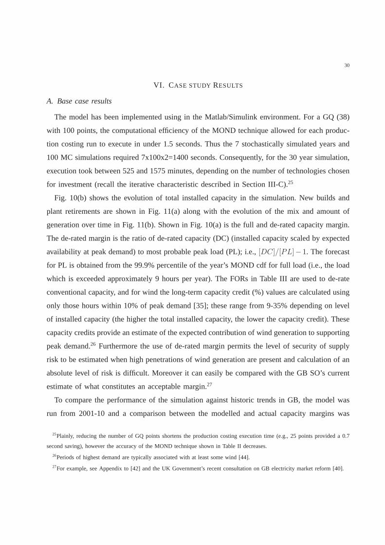
Fig. 10(b) shows the evolution of total installed capacity in the simulation. New builds and

plant retirements are shown in Fig. 11(a) along with the evolution of the mix and amount of

generation over time in Fig. 11(b). Shown in Fig. 10(a) is thefull and de-rated capacity margin.

The de-rated margin is the ratio of de-rated capacity (DC) (installed capacity scaled by expected

availability at peak demand) to most probable peak load (PL); i.e., [DC]/[PL]−1. The forecast

for PL is obtained from the 99.9% percentile of the year’s MOND cdf for full load (i.e., the load

which is exceeded approximately 9 hours per year). The FORs inTable III are used to de-rate

conventional capacity, and for wind the long-term capacitycredit (%) values are calculated using

only those hours within 10% of peak demand [35]; these range from 9-35% depending on level

of installed capacity (the higher the total installed capacity, the lower the capacity credit). These

capacity credits provide an estimate of the expected contribution of wind generation to supporting

peak demand.26 Furthermore the use of de-rated margin permits the level of security of supply

risk to be estimated when high penetrations of wind generation are present and calculation of an

absolute level of risk is difficult. Moreover it can easily becompared with the GB SO’s current

estimate of what constitutes an acceptable margin.27

To compare the performance of the simulation against historic trends in GB, the model was

run from 2001-10 and a comparison between the modelled and actual capacity margins was

25Plainly, reducing the number of GQ points shortens the production costing execution time (e.g., 25 points provided a 0.7

second saving), however the accuracy of the MOND technique shown inTable II decreases.

26Periods of highest demand are typically associated with at least some wind[44].

27For example, see Appendix to [42] and the UK Government’s recent consultation on GB electricity market reform [40].

31

(a)

(b)

Fig. 10. (a) Plot of simulated de-rated and full capacity margins. Historictheoretical GB capacity margins (2001-10) derived

using data from [42] and [45]. (b) Plot of simulated capacity growth. Historic ’actual’ capacity (2001-10) derived using data

from GB SO’s Winter Outlook reports [42].

performed.28 The comparison shows that simulated margins do not perfectly match historic

trends in all years (e.g., 2002/3), however there is a reasonably good agreement of our model

with reality, which gives a degree of confidence in the realism of our future projections. Note

28See [24] for cost and initial capacity data.

32

(a)

(b)

Fig. 11. (a) Plot of simulated new builds and retirements over time. Negative bars indicate plant retirements and positive bars

indicate new builds. Also shown are historic new builds (all CCGT) for 2001-09 (columns labelled ‘CCGT DUKES’ [46]). (b)

Plot of total installed capacity over time, i.e., the result of the mix and amount of generation investment and retirements over

time.

that the “historical theoretical de-rated margin” is what the forecast de-rated margin would have

been for a given winter using the assumptions about plant availability and winter peak load.

This data can be obtained from the GB SO’s Winter Outlook reports (e.g., [42]). Furthermore,

33

the comparison of available historical data on capacity additions plotted in Fig. 11(a) shows that

the CCGT investments triggered by the simulation (columns after 2003) do not correspond in

all years (e.g., 2008) but the volumes and timing are not unreasonably different.

The future trend shows an erosion of de-rated capacity margins after around 2015. This

coincides with the LCPD plant retirements and rapid offshorewind growth. Of the 30 simulated

future years, the average de-rated margin is 5.6% with a standard deviation of 7.1%. De-rated

margins are negative in 4 years, below 5% in 15 years, and below 10% in 25 years. For those

years where margins are below 10%, an average shortfall of 1 GW of capacity was projected. The

UK Government’s recent consultation and subsequent white paper (July 2011) on GB electricity

market reform has stipulated that a peak de-rated margin of 10% provides an acceptable level

of generation adequacy risk [40]. Further, the GB SO has recently stipulated that a de-rated

capacity margin of 5 GW over expected peak demand is desirable (see Appendix to [42]). These

simulation results suggest that a lower than desirable level of adequacy risk could potentially

occur.

The annual LOLE and EEU was also calculated (cf. Section IV-A). The average annual LOLE

across the 30-year simulation was 0.03 hrs/yr with a standard deviation of 0.05, and average

annual EEU of 5.7 GWh (less than 0.002% of typical year’s totalannual energy demand). The

yearly LOLE together with the volume of hypothetical additional capacity required to meet a 5

GW de-rated capacity margin at peak is plotted in Fig. 12.29 The graph shows how the LOLE

is higher in some years, particularly in 2023-26, which is reflected in the de-rated peak margin

shortfall. To put these figures in context, an historic generation adequacy risk calculation is

required; this will allow performance relative to historiclevels of risk to be assessed. However

this analysis is beyond the scope of this paper. Further, theMOND representation is less accurate

for the tails of the distribution and so these risk indices should interpreted with caution. With

this in mind, the values for LOLE and EEU are used primarily toassess the changes in relative

levels of risk over the simulation time horizon and to benchmark the sensitivity analyses described

below rather than to predict absolute levels of system risk.

These projected risk and de-rated capacity margin figures suggest that the system may ex-

perience tight supply conditions during peak demand in someyears. Some of these results can

29A value of zero implies that de-rated margin is in excess of 5 GW.

34

Fig. 12. Plot of simulated LOLE (bars) and capacity shortfall over 5 GW de-rated capacity margin (solid line).

perhaps be explained by inspection of the residual load histograms from Fig. 9(b); the shape

of the right-most tail suggests that even with very high penetrations, wind power does not

contribute in all high demands periods. However the frequency of these high-demand/low-wind

periods is too low to justify investment by private investors. And it is these very high-demand

hours when the potential for a capacity shortfall is highest(excluding here SO actions such as

voltage reductions). From a policy perspective, it is arguably uneconomical to design policies

aimed at ensuring there is adequate generating resource available for these low-frequency events;

an alternative approach would be to encourage demand-side participation through smart grids

and smart metering. However these mechanisms will introduce price dynamics not currently

witnessed in most liberalised energy markets and thereforecareful consideration of the impact

of demand response on generator’s anticipated energy market revenues is required. However this

consideration is beyond the scope of our investigation.

Further, an analysis of generator revenues shows symptoms of a boom and bust investment

cycle. Simulated OCGT total gross margins, which include annualised capital costs (cf. Table III),

are plotted in Fig. 13. Also shown are the triggered investments in this technology. Recall here

that investors stochastically simulate 7 years of prices, so the largest investment years (2017/18)

include the forecast prices for (2023-25), the period when gross margins are highest. However

35

Fig. 13. Plot of simulated total gross margins for OCGT capacity (solid line,left axis). Also shown are the OCGT investment

and mothballing amounts over time (black bars, right axis).

investment reduces in 2019-22 in response to expectations about prices being dampened (although

not sufficiently to prevent an overshoot) as new investment in OCGT and other technologies enter

the system. It is easy to see the pattern of high gross marginscorresponding to those years where

adequacy risk is highest (cf. Fig. 12). The graph shows how the boom in OCGT investment in

expectation of the high gross margins after 2023 is followedby a bust phase around 2026 when

large volumes of new nuclear capacity begin entering the system (cf. Fig. 11(b)). This increases

the capacity margin but reduces profitability for peaking units. In fact, a significant volume of

plant is mothballed toward the end of the simulation time horizon suggesting that generators

expect energy market revenues to remain low.

The mothballing of OCGT early in the simulation (2011) is likely to be a direct result of

unrealistically high capacity margins out to 2014 (cf. Fig.10(b)); the existing CCGT builds

come online during these years in anticipation of LCPD closures (cf. Section V). To avoid over

complicating the plots, the profitability of other technologies is not included, however similar

profitability trends were witnessed for CCGT. Investment in OCGT capacity begins around 2014

with similar trends witnessed in CCGT and nuclear, however no coal investments are made (a plot

of technology screening curves showed coal as uneconomicalrelative to the other technologies).

36

After 2025, very little CCGT or OCGT investment is triggered andendogenous capacity

growth is minimal. Nuclear plants experience a sustained period of positive gross margins after

2023, which is attributed to the rising fuel and carbon costswitnessed for fossil-fuel technologies

(DECC central case estimates) and hence increasing scarcityrents. Combining this with the data

presented in Fig. 11(a), implies a period of intense CCGT and OCGT investment for the 10

years after 2015 to offset retirements to existing capacityand respond to demand growth during

2020-25. Average annual endogenous capacity growth is -2.2% between 2015-25 as a result of

29.7 GW of new thermal build being offset by 42.2 GW of thermalplant retirements (options

for lifetime extension not considered here). This suggeststhat thermal capacity is not replaced

on a like-for-like basis, which is hardly surprising given that average growth in installed wind

generation is 12% over the same period. The ten years after 2025 provide better growth (average

endogenous capacity growth 1.2% between 2026-35), on account of wind capacity levelling off,

demand remaining flat and retirements continuing. In fact, nuclear is the only endogenous plant

type to increase in terms of total installed capacity for theperiod 2025-40. This analysis suggests

that new investments struggle to recover fixed costs during the period after 2026 owing to growth

in nuclear capacity within a high wind system dampening energy market revenues for fossil-fuel

generation.

An interesting analysis is to compare simulated real-time (annual) prices with investor expec-

tations. This can be used to determine how well investors predictions of gross margins track

those realised. Fig. 14 shows the average simulated competitive prices across the MC runs versus

realised competitive prices for 1 and 3 years ahead for each of the years 2010, 2015, 2020 and

2025. Choosing 2020 as an example, in Fig. 14(a) (x-axis), theaverage of expected simulated

competitive price for 2021 (solid line with squares) is higher than the realized price for 2021

(dashed line with triangles) by 12£/MWh. The degree of difference is also directly related to the

volume of plant under construction; the more plant being built, the greater the over-estimation

of market prices (and hence gross margins). Furthermore, the proportion of long lead time plant

under construction exacerbates this trait. For instance, in 2020 the volumes of OCGT, CCGT

and nuclear capacity under construction are 3.9, 5.8 and 3 GW, respectively, where as in 2025

it is 0, 10 and 6.5 GW, respectively, which is the year with thebiggest difference. Note that,

although mark-ups from market power are not shown here, precisely the same pattern occurs for

simulated revenues from mark-ups. This can be traced back tothe degree of uncertainty with

37

which plant under construction is treated by the investor; the exact timings of when new plants

will arrive are modelled as stochastic (cf. Section III-A).To test this hypothesis, a sensitivity

case was modelled where investors have perfect foresight about investments in the pipeline, this

is described in the next section (case 2c).

(a)

(b)

Fig. 14. (a) Plot of expected competitive market prices 1 year ahead from decision year (x-axis) and (b) expected competitive

market prices 3 years ahead from decision year. Volume of capacity under construction at time decision is taken also shown in

each case (columns).

38

B. Sensitivity analyses

In order to test the robustness of the model, extensive sensitivity analyses have been performed

on a number of model assumptions. Those found to be the most critical, some of which are plotted

in Fig. 15 with key associated metrics shown in Tables IV and V, include:

1) The level of expected scarcity price (i.e., VOLL). Here, the maximum value of 10,000£/MWh

is reduced and the price mark-up functionw(L,G∗N) is altered (cf. Fig. 7(b)) when

calculating expected gross margins (37). Experiments using case a) VOLL 30000’: 30,000

£/MWh and b) ‘VOLL 2000’: 2,000£/MWh are carried out.

2) Investor expectations about new builds. Taking inspiration from [6], we test case a) the

‘believers’ case; here the investor ignores plants under construction when making expec-

tations about revenues. The impact of new builds on prices are only considered once

plants are fully operational (i.e., will systematically over-predict market prices). Secondly,

case b), the‘pre counter’ is used where the investor views all plant under construction

as operational (i.e., will systematically under-predict market prices). Finally, case c), a

’accurate’ investor is modelled where estimates about construction lead times match the

delays experienced in reality (i.e., lead times shown in Table III). This last case can be

used to test the hypothesis that differences between realised and investor expectations about

prices is due to the uncertainty surrounding capacity underconstruction.

3) The aggregate investment response from the market. This is achieved by altering the

constant exponent,β, in the aggregate investment response function (9) to a) 0.9, ‘Resp.

higher’ and b) 0.5,‘Resp. lower’ (cf. Fig. 2).

4) The ability of plant owners to exercise market power and volumes of revenues received by

doing so, reference ‘No markup’. This is achieved by calculating expected gross margins

using (24) instead of (37) (i.e., no price mark-up and a perfectly competitive market).

5) Investor risk preferences: achieved by case a) ‘VaR higher’: increasing criticalq to 0.5

in VaR test (cf. Section III-B), case b) ‘VaR lower’: lowering critical q to 0.01, case c)

‘WACC lower’: reducing investor WACC and case d) ‘WACC higher’:increasing investor

WACC.

6) Increasing investor uncertainty about load growth. Investors still consider load growth to

be stochastic, however the standard deviation of the Normaldistribution used to sample

39

load growth is increased from 1% to 3%, reference ‘Load SD’.

7) Economics of peaking plants: achieved by case a) ‘AS reduce’: reducing the amount of

AS revenue for OCGT plants and case b) ‘FC increase’: increasing total fixed costs (i.e.,

TAFCx).

Fig. 15. Plot of simulated LOLE for selected sensitivities (nos. 1-6). Notethe logarithmic scale.

Overall, the model’s qualitative behaviour was reasonablefor the sensitivities listed and

provided some useful insights, particularly when comparing the oligopolistic base case to the

perfectly competitive market results (i.e., zero price mark-up, see below).

For test case ‘VOLL 30000’, by increasing the VOLL, the expectation would be to see more

investment as price spikes signals are stronger, which could potentially lead to a lower level of

risk and also more investment relative to the base case. For test case ‘VOLL 2000’, by reducing

the VOLL, the expectation would be to see delays in investment as price spikes are dampened,

which could potentially lead to a higher level of risk and also less investment relative to the base

case. For instance, in a perfectly competitive market, in order for an OCGT plant to recover

40

TABLE IV

FIRST SUMMARY TABLE OF SECURITY OF SUPPLY AND INVESTMENT RESULTS FOR BASE CASE AND SENSITIVITY

ANALYSIS . FIGURES IN BRACKETS BELOW EACH CASE FIGURE SHOW STANDARD DEVIATION (SECURITY OF SUPPLY RISK

METRICS) OR VOLUME OF PLANT MOTHBALLED (TOTAL INVESTMENT AND MOTHBALLING ).

Security of supply risk metrics Total investment and mothballing

Average Average No. years Deepest LOLE EEU 2010-40

de-rated diff. in negative shortfall (hrs/yr) (GWh) (GW)

margin margins (%,yr)

2010-40 relative

Test (%) to base

case (%) Nuclear Coal CCGT OCGT

Base case 5.6 - 4 (-6.8, 2024) 0.03 5.7 30.5 0 34 12.1

(7.1) (0.05) (9.2) - (3.0) (1.2) (4.6)

VOLL 30000 6.5 1.2 1 (-1.3, 2025) 0.02 3.3 31.5 0 37 15

(5.0) (0.02) (3.1) - (2.5) (7.8) (10.9)

VOLL 2000 3.8 -3.0 10 (-9.0, 2022) 0.22 46.8 30.5 0 32.6 13.3

(7.8) (0.49) (116.7) - (3.0) (3.0) (5.0)

Believer 12.9 7.0 1 (-2.6, 2018) 0.01 1.9 30.5 0 34 32.4

(6.7) (0.02) (4.8) 0 (3.5) 0 (15.0)

Pre counter -5.1 -10.1 21 (-16.9, 2026) 0.71 158.7 30.5 0 27.6 12.0

(8.5) (0.70) (167.3) - (3.0) (3.6) (5.3)

Accurate 1.7 -3.9 15 (-5.9, 2030) 0.06 10.2 31.0 0 24.2 22.9

(4.5) (0.05) (8.3) - (1.5) (3.6) (6.2)

Resp. higher 6.3 0.8 6 (-4.7, 2024) 0.02 4.0 31.0 0 36.8 13.7

(5.2) (0.03) (5.3) - (3.0) (5.8) (6.6)

Resp. lower 5.0 -0.5 8 (-5.8, 2023) 0.05 8.9 29.0 0.5 35.2 19.8

(5.7) (0.08) (14.3) - (2.5) (1.0) (4.9)

No markup -8.3 -13.0 20 (-33.2, 2024) 3.9 1474 31.0 0 32.6 8.5

(14.4) (6.25) (2621.2) - (1.0) (0.6) (1.4)

41

TABLE V

SECOND SUMMARY TABLE OF SECURITY OF SUPPLY AND INVESTMENT RESULTS FOR BASE CASE AND SENSITIVITY

ANALYSIS . FIGURES IN BRACKETS BELOW EACH CASE FIGURE SHOW STANDARD DEVIATION (SECURITY OF SUPPLY RISK

METRICS) OR VOLUME OF PLANT MOTHBALLED (TOTAL INVESTMENT AND MOTHBALLING ).

Security of supply risk metrics Total investment and mothballing

Average Average No. years Deepest LOLE EEU 2010-40

de-rated diff. in negative shortfall (hrs/yr) (GWh) (GW)

margin margins (%,yr)

2010-40 relative

Test (%) to base

case (%) Nuclear Coal CCGT OCGT

Base case 5.6 4 (-6.8, 2024) 0.03 5.7 30.5 0 34 12.1

(7.1) (0.05) (9.2) - (3.0) (1.2) (4.6)

VaR higher 7.3 1.7 4 (-5.3, 2023) 0.02 3.4 29.5 0 30.6 18.2

(5.2) (0.03) (5.1) - (3.5) (2.8) (6.4)

VaR lower 6.2 0.9 5 (-5.7, 2023) 0.02 4.2 30 0 31 16.6

(5.0) (0.03) (6.1) - (3.0) (3.6) (7.1)

WACC lower 7.0 1.4 4 (-4.9, 2023) 0.02 3.3 30.5 0 28.4 7.8

(4.8) (0.03) (4.8) - (3.0) (1.0) (1.6)

WACC higher 4.8 -0.8 7 (-5.5, 2023) 0.03 5.8 31.5 0 39.2 19.1

(4.6) (0.04) (7.5) - (3.0) (1.4) (4.7)

Load SD 8.5 2.9 3 (-1.9, 2026) 0.01 2.0 30.5 0 32.4 22.6

(5.3) (0.01) (2.4) 0 (2.0) (0.8) (6.7)

AS reduce 3.9 -1.6 12 (-6.9, 2023) 0.05 9.3 31 0 39.2 9.9

(5.0) (0.07) (12.5) - (3.0) (5.0) (5.1)

FC increase 5.9 0.0 5 (-4.1, 2023) 0.04 7.4 30.5 0 38.8 12.8

(4.3) (0.04) (7.1) - (3.0) (3.0) (14.3)

its fixed costs (47.25£/unforced kW/yr), the price must reach the VOLL (10,000£/MWh) in

at least 4.7 hrs/yr (actually more to account for short-run MC of production), and reducing the

VOLL to 2,000 £/MWh increases this duration to 23.6 hrs/yr. The simulation results showed

that increasing the VOLL to 30,000£/MWh leads to a small improvement in average de-rated

margins to 6.5% with a standard deviation of 5.0%. Furthermore, de-rated margins are negative

42

during only 2026/27. The average annual LOLE reduces to 0.02hrs/yr with average annaul EEU

of 3.3 GWh. Interestingly, CCGT investment begins 1 year earlier and has a smoother cumulative

profile relative to the base case (standard deviation of year-on-year volumes 0.8 GW versus 1.2

GW in base case). This displaces some OCGT investment early on, but overall volume during

2015-25 increase by 2 GW. Reducing the VOLL to 2,000£/MWh alters investment timings, but

overall volumes are only slightly reduced (3% lower than base case). The average annual LOLE

increases to 0.22 hrs/yr with average annaul EEU of 46.8 GWh. CCGT investment starts 2 years

later relative to the base case, which interestingly increases nuclear investment by 2 GW during

2015-20. OCGT investment is less intense during 2015-18 but volumes are significantly higher

during 2020-23 (4.7 GW compared with 1.1 GW). This is in response to higher expected gross

margins in 2022-26 as a result of less short lead time plant investment early on.

For test case‘believers’, the anticipation would be more investment relative to the base case

due to the investor now systematically over-estimating revenues because they do not account for

the impact of new builds when formulating price expectations. Results produced more investment

than under the base case, with more severe over-shoot dynamics witnessed. As a result, average

annual LOLE falls to 0.01 hrs/yr with generators unable to recover fixed costs with significant

increases in the volume of mothballed OCGT capacity.

For test case‘pre counters’, the anticipation would be less investment relative to the base case

due to the investor now systematically under-estimating revenues because they include new builds

before they are operational when formulating their price expectations. Results showed under-

investment and average annual LOLE increases to 0.71 hrs/yr. As a result of less investment,

overall profitability of existing plant improves, with somemothballing in the early part of the

simulation in response to high forecast margins.

For test case‘accurate’, the expectation would be reduced over-shoot dynamics and better

prediction of out-turn prices relative to the base case. This is on account of the investor making

a better prediction of the timing of capacity under construction, which is particularly important

when there is a lot of long lead time plant (e.g., nuclear) under construction. Simulation results

show that nuclear, CCGT and OCGT receive positive gross marginsin almost all years after 2015,

however average LOLE doubles to 0.06 hrs/yr and with a noticeable oscillation of frequency

5 years and amplitude 0.12 hrs/yr (Fig. 15). Average EEU alsoincreases to 10.2 GWh. Fig.

14 shows a significant improvement in investor price expectations at the 1 year ahead stage,

43

with expectation 3 years ahead also more akin to reality. Expectations about years 4-7 ahead

performed better than the base case, however, due to the possibility of new investments (or

mothballing) impacting on those years, significant differences remain.

For test case ‘Resp. lower’, the expectation would be that reductions to the exponentβ in (9)

to reduce investment, and increases under ‘Resp. higher’ to increase investment. This could also

impact on the timing of investments later in the simulation in account of changes to investment

levels early on. The results followed expectations; changes produced similar investment timings

to the base case for OCGT and CCGT early in the time horizon but thereduced (resp. increased)

levels of aggregate response lead to increases (resp. decreases) in generation adequacy risk in

the medium-term (out to 2020) but higher (resp. lower) levels of investment later on in response

to higher (resp. lower) forecast revenues. In the case of nuclear, a reduced response curve time-

slipped the investment pattern by two years from 2020, whereas for the increased response curve

the patterns were broadly similar.

For test case ‘No markup’, the perfectly competitive marketcase, the expectation would be

lower overall levels of investment on account of price mark-ups being removed from the revenue

calculation. Here more sustained periods of high prices (and hence scarcity rents) are required

in order to recover invested capital and receive adequate return on investment. Indeed, when

limiting the ability to exercise market power by removal of price mark-up, CCGT investments

are most affected. Investment in this technology starts four years later than the base case and

cumulative investment is on average 4.4 GW lower. Nuclear investments are also dampened,

with investment during the first 15 years of the simulation 3 GW lower than the base case.

These dynamics led to an order of magnitude increase in average annual LOLE and EEU to 3.9

hrs/yr and 1474 GWh, respectively. Of course these dynamics may differ in a model representing

more sophisticated firms who account for the effect of their investment upon mark-ups for their

existing fleet. In this case firms may deliberately not investin order to keep prices (including

mark-ups) high, however this type of investor logic is not considered here.

For test case ‘VaR higher’ and ‘VaR lower’, the expectation would be to see changes to the

level of investments, particularly early on when the threshold for investment, which is considered

only if the VaR criterionp(V qx > 0) ≥ (100− q)% is met. This means that an investment could

be deemed attractive earlier (in the case whereq = 0.5) or later (in the case whereq = 0.01)

relative to the base case. Moreover, the VaR criterion relates to the degree of risk aversion (cf.

44

Section III-B), thereforeq = 0.5 models a less risk averse investor, andq = 0.01 models a

more risk averse investor. Results of this experiment showedthat modelling a less risk averse

investor leads to marginally earlier nuclear investment (typically viewed as high risk due to high

investment costs and operational inflexibility), with peaking plant investment timings remaining

unchanged but volumes increasing in some years. Modelling amore risk averse investor leads

to OCGT investment timings remaining unchanged but volumes increasing and displacing some

CCGT (5.4 GW overall reduction in CCGT and 3.3 GW increase in OCGT);this is attributed to

a higher degree of certainty about prices in the near term, resulting in less variance in projected

revenues for short lead time plant. Hence the VaR criterion will tend to favour this type of plant

for low values ofq.

For test case ‘WACC lower’ and ‘WACC higher’, a similar expectation to that of ‘VaR higher’

and ‘VaR lower’ were held. Results show that the degree of impact that changes to the WACC

had on investment timings was related to construction lead time. This is hardly surprising given

that investment costs for long lead time plant are highly sensitive to the discount rate used. For

instance, increasing required equity by 3% across all technologies delays nuclear investment by

3 years and overall volume by 5.5 GW during 2010-25. This leads to higher generation adequacy

risk during 2018-22. Similarly, CCGT investments are delayedby 2 years although volumes are

similar in account of the lower nuclear builds increasing expected gross margins and triggering

investment. Reducing the equity return by 3% leads to higher and earlier volumes of nuclear

investment with annual average LOLE reduced, however grossmargins are reduced.

For test case ‘Load SD’, the expectation would be that an increase to the standard deviation

of load growth to lead to a higher standard deviation of the distribution of project value. This

increased uncertainty surrounding profitability would reduced and/or delay investment. In fact,

increasing investor load growth uncertainty leads to less CCGT and nuclear investment out to

2020, however OCGT investment increases by 10 GW over the basecase for the period 2019-21

in anticipation of high market prices in 2022-26. This high volume of investment lowers the

generation adequacy risk and serves to dampen market prices, and OCGT gross margins are

positive in 2026 only (the only year when de-rated margins are negative).

For test case ‘AS reduce’, a reduction in AS revenues (and hence profitability) was expected

to reduce OCGT investments, although not massively in account of AS revenues alone not being

sufficient to trigger investment (cf. Section III-A). In fact, reducing OCGT AS revenues from

45

10,000/MW/yr to 5,000/MW/yr alters investment timings and capacity choice early on in the

simulation, however long-term overall volumes are only marginally affected. More precisely, a

reduction in OCGT investment during 2014-2018 (1.6 GW compared with 11 GW in base case)

is somewhat offset by increases in CCGT (8.8 GW compared with 4.6 in base case) and nuclear

(up 2.5 GW on base case) investment during this period. All three technologies were deemed

profitable during this period; the model chooses the technology with the highest PI (10) and

iterates until no additional plants are profitable (cf. Section III-C). A reduction in AS revenues

for OCGT means that other technologies have more favourable profitability in the first iteration

of the investment decision. OCGT is not chosen in subsequent iterations as a result of other

capacity additions reducing its profitability to suboptimal levels. By choosing to invest in longer

lead time plant, total LOLE over 2019-2023 increases from 0.29 to 0.97 hrs. Interestingly, higher

volumes of OCGT investment occur in these later years (5.6 GW during 2019-2020 compared

with 1.1 GW in base case). This is likely to be a consequence ofthe increased volumes of longer

lead time plant under construction during this period increasing the differences between investor

price predictions and reality (i.e., as discussed in sensitivity 2c).

Finally, for case ‘FC increase’, increasing OCGTTAFCx from 42.5 to 60£/MW/yr was

expected to produce similar dynamics to ‘AS reduce’. This turned out to be the case, however

the increase in LOLE is less severe (although still higher than the base case).

In summary, a pattern of increased relative levels of risk and erosion of de-rated capacity

margins was experienced during the 2020s to some degree in all cases. Furthermore, the period

of highest security of supply risk is 2023-28, however the magnitude of the risk (measured by

LOLE) differs between experiments. A prolonged period of increased security of supply risk

is experienced throughout the 2020s for the perfectly competitive market case. Also, providing

investors with perfect foresight about capacity under construction produces less investment and

more frequent periods of relatively high LOLE and low de-rated margins after 2020. However,

generators experience positive gross margins in more yearson account of reduced surplus

margins, and hence higher prices.

The 2020s is the period of most intense change; during this decade over 40 GW of new

capacity is built with over 34 GW retiring; 14.5 GW of capacity leaves the system during the

period 2023-26 alone. This further exacerbates the higher relative levels of risk during this period.

Furthermore, no new coal investments are made, with the majority of new investment coming

46

from gas-fired generation. That said, however, a sensitivity on the primary fuel prices is not

included here. For instance, lower coal prices (or indeed higher gas prices) may lead to different

technology choice, however the impact on overall volumes (and hence relative levels of risk) is

likely to remain unchanged.

VII. C ONCLUSION

The MOND technique to calculate expected output, costs and revenues of thermal generation

subject to varying load and random independent thermal outages has been presented. This

method has been adapted for use in a dynamic capacity market model with high penetrations of

wind by performing a residual load calculation with simulated wind outputs. An ‘energy-only’

market setting has been used to estimate the economic profitability of capacity investments.

Using relative levels of de-rated capacity margin and LOLE as the risk metric, simulation

results for GB show that levels of generation investment lead to a mild increase in generation

adequacy risk in some years, with erosion of de-rated capacity margins in the mid 2020s, and

very tight supply conditions are experienced during a smallnumber of peak hours. Many new

investments, particularly peaking units, were unable to recover their fixed costs. A sensitivity

analysis demonstrated that assumptions about investor risk profiles and expectations about new

builds, load growth and the ability to exercise market powerhave a strong impact on simulated

investment dynamics and subsequent levels of generation adequacy risk. However a relative

increase in generation adequacy risk in the mid 2020s was experienced across all experiments,

with increases occurring earlier and more severely in some cases.

A key goal for policy makers is to ensure that liberalised energy markets incentivise timely and

sufficient thermal generating capacity investment in orderto compliment increasing penetrations

of variable output generation such as wind. This is particularly true of peaking generation and

energy storage technologies. Due to their low utilisation factors, these units will rely on being

dispatched at high prices in order to recover their fixed costs and provide adequate returns

on investment. Results presented here suggest that revenuesfrom an ‘energy-only’ market

are insufficient and additional mechanisms may be required.Moreover a sensitivity analyses

demonstrated that investor expectations about wholesale prices, in particular the demand-side’s

willingness to pay and the damping effect that new builds have on revenues, exacerbate the risk

of investment shortfalls. This has significant policy implications for GB where sizeable demand

47

response and new smart-loads are expected to emerge. Whetheror not these entities will in

fact respond to high wholesale prices by reducing consumption remains to be seen. However

if generators anticipate a price responsive demand-side and it fails to emerge, then a relative

increase in the risk of investment shortfall is likely to occur.

The topic of subsequent research will be to determine whether explicit capacity mechanisms

such as tendering for strategic reserve (e.g., [40]) and capacity markets (e.g., [14]) can be

designed to alleviate resource shortfall and prevent investment overshoot. The results here indicate

that such a mechanism may be desirable to improve reserve margins in the mid 2020s in GB.

ACKNOWLEDGMENT

The authors acknowledge valuable input from C. Dent, S. Hawkins, T. Johnson and G. P.

Harrison. Also thanks to EPRG, in particular D. Newbery, for facilitating this collaboration.

This research formed part of the UKERC programme and was supported by the UK Research

Councils under NERC award NE/C513169/1. Partial support for B.F. Hobbs was provided by

the U.K. EPSRC Supergen Flexnet program and the U.S. NationalScience Foundation through

EFRI Grant 0835879.

REFERENCES

[1] H. Baleriaux, E. Jamoulle, and F. Linard de Guertechin, “Simulation de L’Explotation d’un Parc de Machines

Thermiques de Production D’Electricite Couple a des Stations de Pompage,”Revue E de la Societe Royale

Belge des Electriciens, vol. 7, pp. 225–245, 1967.

[2] R. Booth, “Power System Simulation Model Based on Probability Analysis,” IEEE Trans. Power Apparatus

and Systems, vol. PAS-91, no. 1, pp. 62–69, Jan. 1972.

[3] G. Gross, N. Garapic, and B. McNutt, “The Mixture of Normals Approximation Technique for Equivalent

Load Duration Curves,”IEEE Trans. Power Systems, vol. 3, no. 2, pp. 368–374, May 1988.

[4] J. G. Inon, “Long-run Probabilistic Production Costing-Based Analysis of Electricity Market Designs for Long-

Run Generation Investment Incentives under Spot-Pricing and Transmission Open-Access,” Ph.D. dissertation,

John Hopkins University, 2011, in preparation.

[5] B. F. Hobbs, J. Inon, and S. E. Stoft, “Installed Capacity Requirements and Price Caps: Oil on the Water, or

Fuel on the Fire?”The Electricity Journal, vol. 14, no. 6, pp. 23 – 34, 2001.

[6] A. Ford, “Waiting for the Boom: a Simulation Study of Power Plant Construction in California,”Energy

Policy, vol. 29, no. 11, pp. 847 – 869, 2001.

[7] S. Gary and E. R. Larsen, “Improving Firm Performance in Out-of-Equilibrium, Deregulated Markets Using

Feedback Simulation Models,”Energy Policy, vol. 28, pp. 845–855, 2000.

48

[8] F. Olsina, F. Garces, and H.-J. Haubrich, “Modeling Long-Term Dynamics of Electricity Markets,”Energy

Policy, pp. 1411–1433, 2006.

[9] T. Kayoda, S. Ihara, E. Larose, M. Sanford, A. K. Graham, C. A. Stephens, and C. K. Eubanks, “Utilizing

System Dynamics Modeling to Examine Impact of Deregulationon Generation Capacity Growth,” in

Proceedings of the IEEE, vol. 93, no. 11, Nov 2005.

[10] B. Hobbs and Y. Ji, “A Bounding Approach to Multiarea Probabilistic Production Costing,”IEEE Trans.

Power Systems, vol. 10, no. 2, pp. 853 –859, May 1995.

[11] A. Bar-Ilan, A. Sulem, and A. Zanello, “Time-to-build and Capacity Choice,”Journal of Economic Dynamics

and Control, vol. 26, no. 1, pp. 69–98, January 2002.

[12] E. R. Larsen and D. W. Bunn, “Deregulation in Electricity: Understanding Strategic and Regulatory Risk,”

The Journal of the Operational Research Society, vol. 50, no. 4, pp. 337–344, April 1999.

[13] J. F. Muth, “Rational Expectations and the Theory of Price Movements,”Econometrica, vol. 29, no. 3, pp.

315–335, July 1961.

[14] B. F. Hobbs, M.-C. Hu, J. G. Inon, S. E. Stoft, and M. P. Bhavaraju, “A Dynamic Analysis of a Demand

Curve-Based Capacity Market Proposal: The PJM ReliabilityPricing Model,” IEEE Trans. Power Systems,

vol. 22, no. 1, pp. 3 –14, Feb. 2007.

[15] Department of Energy and Climate Change, “Communication on DECC Fossil Fuel Price Assumptions,”

www.decc.gov.uk/en/content/cms/about/ecsocial res/analyticprojs/ff prices/ff prices.aspx.

[16] ——, “First Annual Update of the Short Term Traded Carbon Values (June 2010),” www.decc.gov.uk/en/

content/cms/whatwe do/lc uk/valuation/valuation.aspx.

[17] ICE Futures Europe, “Report Center; End of Day Reports (UK Natural Gas & Newcastle Coal Futures),”

www.theice.com/marketdata/reports/ReportCenter.shtml.

[18] A. Cartea and M. Figueroa, “Pricing in Electricity Markets: a Mean Reverting Jump Diffusion Model with

Seasonality,” EconWPA, Finance 0501011, Jan. 2005.

[19] A. Dixit and R. Pindyck,Investment Under Uncertainty. Princeton University Press, 1994.

[20] “Our Electricity Transmission Network: A Vision for 2020,” ENSG, Tech. Rep., www.ensg.gov.uk/index.php?

article=126.

[21] World Nuclear Association, “The Economics of Nuclear Power,” www.world-nuclear.org/info/inf02.html.

[22] “UK Electricity Generation Costs Update,” Mott MacDonald, Tech. Rep., June 2010, www.decc.gov.uk/en/

content/cms/about/ecsocial res/analyticprojs/gencosts/gencosts.aspx.

[23] P. Artzner, F. Delbaen, J.-M. Eber, and D. Heath, “Coherent Measures of Risk,”Mathematical Finance, vol. 9,

no. 3, pp. 203 – 228, 1999.

[24] D. Eager, J. W. Bialek, and T. Johnson, “Validation of a Dynamic Control Model to Simulate Investment

Cycles in Electricity Generating Capacity,” inPower and Energy Society General Meeting, 2010 IEEE, July

2010, pp. 1–8.

49

[25] R. Billinton and R. N. Allan,Reliability Evaluation of Power Systems. 2nd ed.Plenum, 1994.

[26] J. Endrenyi,Reliability Modeling in Electric Power Systems. Wiley, 1978.

[27] S. Stoft,Power System Economics Designing Market for Electricity. IEEE Press: Wiley, 2002, pp. 70–71.

[28] J. Boucher and Y. Smeers, “Alternative Models of Restructured Electricity Systems, Part 1: No Market Power,”

Operational Research, vol. 49, pp. 821–838, Nov. 2001.

[29] C. Metzler, B. F. Hobbs, and J.-S. Pang, “Nash-Cournot Equilibria in Power Markets on a Linearized DC

Network with Arbitrage: Formulations and Properties,”Networks and Spatial Economics, vol. 3, pp. 123–150,

2003.

[30] Poyry, “Impact of Intermittency: How Wind Variability CouldChange the Shape of the British and Irish

Electricity Markets,” July 2009, www.poyry.com/linked/group/study.

[31] R. Sioshansi and S. Oren, “How Good are Supply Function Equilibrium Models: an Empirical Analysis of

the ERCOT Balancing Market,”Journal of Regulatory Economics, vol. 31, pp. 1–35, 2007.

[32] J. B. Bushnell, E. T. Mansur, and C. Saravia, “Vertical Arrangements, Market Structure, and Competition: An

Analysis of Restructured US Electricity Markets ,”American Economic Review, vol. 98, no. 1, pp. 237–66,

2008.

[33] P. Visudhiphan, “Dynamic Investment in Electricity Markets and Its Impact on System Reliability,” inMarket

Design 2001 Conference, Stockholm, 2001, pp. 91–110.

[34] J. Valenzuela and M. Mazumdar, “Cournot Prices Considering Generator Availability and Demand Uncer-

tainty,” IEEE Trans. Power Systems, vol. 22, no. 1, pp. 116 –125, Feb. 2007.

[35] P. E. O. Aguirre, C. J. Dent, G. P. Harrison, and J. W. Bialek, “Realistic Calculation of Wind Generation

Capacity Credits,” inIntegration of Wide-Scale Renewable Resources Into the Power Delivery System, 2009

CIGRE/IEEE PES Joint Symposium, July 2009, pp. 1–8.

[36] Personal communication S. Hawkins and G. P. Harrison, Institute for Energy Systems, University of Edinburgh.

[37] Met Office Unified Model, www.metoffice.gov.uk/science/creating/daysahead/nwp/um.html.

[38] S. Hawkins, D. Eager, and G. P. Harrison, “Characterising the Reliability of Production from Future British

Offshore Wind Fleets,” inRenewable Power Generation Conference, 2011. IET, to be published in 2011.

[39] RenewableUK, www.bwea.com/offshore/index.html.

[40] Department of Energy and Climate Change, “ElectricityMarket Reform Consultation Document,” Tech. Rep.,

December 2010, www.decc.gov.uk/en/content/cms/consultations/emr/emr.aspx.

[41] “Seven Year Statements,” National Grid, Tech. Rep., www.nationalgrid.com/uk/Electricity/SYS/.

[42] “Winter Outlook Consultation 2010/11,” National Grid, Tech. Rep., www.nationalgrid.com/uk/Gas/TYS/

outlook/.

[43] Department of Energy and Climate Change, “Energy and Emissions Projections,” www.decc.gov.uk/en/content/

cms/about/ecsocial res/analyticprojs/en emis projs/en emis projs.aspx.

[44] S. Zachary, C. Dent, and D. Brayshaw, “Challenges in Quantifying Wind Generation’s Contribution to Securing

50

Peak Demand,” inPower and Energy Society General Meeting, 2011 IEEE, July 2011, pp. 1 –8.

[45] Economic and Social Data Service, www.esds.ac.uk/international/access/datasetoverview.asp#descieaei.

[46] Digest of United Kingdom Energy Statistics, “Chapter 5: Electricity, Tables 5.6 and 5.7,” www.decc.gov.uk/

en/content/cms/statistics/publications/dukes/dukes.aspx.

Dan Eager received the B.Sc. degree in mathematics and computer science from The University of Sussex in 2004, and the

M.Sc. degree in operational research from The University of Edinburgh in 2007. He is currently undertaking a Ph.D. within

The University of Edinburgh’s Institute for Energy Systems under the supervision of G. Harrison, J. Bialek and T. Johnson.

Benjamin F. Hobbs received the Ph.D. degree in environmental system engineering fromCornell University, Ithaca, NY, in

1983. He is Schad Professor of Environmental Management at the Johns Hopkins University, Baltimore, MD. In 2009-2010 he

was on sabbatical at the Electricity Policy Research Group at the University of Cambridge. He chairs the California ISO Market

Surveillance Committee and is Director of the JHU Environment, Energy, Sustainability & Health Institute.

Janusz W. Bialek is Professor of Electrical Power and Control with the School of Engineering and Computing Sciences, Durham

University, UK. He holds M.Eng (1977) and Ph.D. (1981) degrees from Warsaw University of Technology, Poland. In 1981-

1989 he was with Warsaw University of Technology, in 1989-2002 with Durham University, UK, and in 2003-2009 with The

University of Edinburgh. He has co-authored 2 books and over 100 technical papers.

51

APPENDIX A

ABBREVIATIONS & FORMULA VARIABLES

A. AbbreviationsAS - Ancillary services

BM - Balancing market

CCGT - Combined cycle gas turbine

cdf - Cumulative distribution function

DDE - Delay Differential Equation

DECC - Department of Energy and Climate Change

DC - De-rated capacity

ELDC - Effective load duration curve

EEU - Expected energy unserved

FOR - Forced outage rate

GQ - Gaussian quadrature

GB - Great Britain

LCPD - Large Combustion Plant Directive

LDC - Load duration curve

LOLE - Loss-of-load Expectation

MOND - Mix of Normals distribution

MC - Monte Carlo

NPV - Net Present Value

PL - Most probable peak load

PJM - Pennsylvania-New Jersey-Maryland

PI - Profitability Index

OCGT - Open cycle gas turbine

r.v. - Random variable

SO - System Operator

WACC - Weighted average cost of capital

VaR - Value at Risk

VOLL - Value of Lost Load

52

B. Formula variablesαx - Operating lifetime (technology typex)

α - Speed of mean reversion

β - Calibrated exponential constant in aggregate investmentresponse function

χ - Gearing ratio

δ(t) - Dirac delta function

ǫ - Required equity investor return

γ - Expected bond return

ηx - Time investment capacity block triggered (technology type x)

µ - Mean of distribution

πi - Wholesale price when generatori is at the margin

ρ - Forced outage rate

σ - Standard deviation of distribution

τx - Build time (technology typex)

ξx - Investment capacity block (technology typex)

ξmax - Maximum annual investment per technology

ψx - Vector of new build capacity blocks (technology typex)

Φ - cdf of Normal distribution

a - Scalar in wholesale price mark-up function

b - Exponent in wholesale price mark-up function

c - Capacity

en - Expected energy served by generator typen

f(M) - pdf of the surplus marginMN

f(MN−1,MN ) - Joint distribution of capacity marginsMN−1 andMN

hn - Probability generatorn is on the margin

ix - Constant used to calibrate aggregate investment responsefunction (technologyx)

mc(L,G1, G2, . . . , GN ) - Marginal production cost of meeting the loadL

mu - Number of units of typen

m(t) - Stochastic process time dependent mean reverting level attime t

px - Construction cost (technology typex)

pdispn - Probability that a MW belonging to generatorn is dispatched

q(t) - DECC fuel price estimate at timet

r - Weighted Average Cost of Capital

v - Integral upper bound in (30), (31), (32), and (31) above which price mark-up is

negligible owing to the large surplus margin

53

w(L,G∗

N ) - Wholesale price mark-up function

Acrfx - Deferred CRF (technology typex)

AGMx - Gross margins over fixed operating costs (technology typex)

Cn(P ) - Total variable operating cost of generator typen, power outputP

CGMn - Expected annual perfectly competitive gross margin

DCx - Present worth of the decommissioning cost (technology type x)

E(Gn) - Expected available capacity from generator typen

FCx - Fixed costs (technology typex)

Ft - Fuel cost at timet

G - Generator expected available capacity

G∗

N - Total available generation

G∗

N − L - Overall capacity margin

GM ix - Expected annual gross margin (technology typex, yeari)

GMn - Expected annual gross margin for generatorn

ICx - Present worth of investment cost (technology typex)

Ix - Installed capacity (technology typex)

I(t) - Total installed capacity at timet

Ln−1(x) - Load still to be met after adding generator typen− 1

Ln(x) - Load still to be met after adding generator typen

LN+1(0) - Probability that there will be insufficient generation to meet demand

MCi - Marginal cost of generatori

Mxi - Capital expenditure vector (technology typex, yeari)

Mn−1 - Surplus margin afterL has been met using all available generation lower in the merit

order thann

N - Total number of psuedo-generators

PIqx - Profitability index (technology typex)

Rin - Expected gross margin for a particular MW of capacity belonging to generatorn when

generatori is at the margin

RL,G∗

N

n - Gross margin received by a MW of capacity from generatorn for loadL and total

available generationG∗

N

RPMn - Expected revenue from price mark-up

TAFCx - Total annualised costs per unforced MW

TIACx - Total interest accumulated during construction

Vx - NPV of an investment (for technologyx)

V optx - Minimal acceptableVx (for technologyx)

W - Standard one-dimensional Brownian motion