dynamic modulus test – laboratory … · 2008-07-15 · the objectives of this study were to...

DYNAMIC MODULUS TEST – LABORATORY INVESTIGATION AND FUTURE

IMPLEMENTATION IN THE STATE OF WASHINGTON

By

MUTHUKUMARAN ANBILPADUGAI ELANGOVAN

A thesis submitted in partial fulfillment of

the requirements for the degree of

MASTER OF SCIENCE IN CIVIL ENGINEERING

WASHINGTON STATE UNIVERSITY

Department of Civil and Environmental Engineering

AUGUST 2008

ii

To the Faculty of Washington State University:

The members of the Committee appointed to examine the thesis of

MUTHUKUMARAN ANBILPADUGAI ELANGOVAN find it satisfactory and

recommend that it be accepted.

___________________________________

Chair

___________________________________

___________________________________

iii

ACKNOWLEDGMENT

I thank my advisor Dr. Laith Tashman for his guidance and support that helped me carry

out this study successfully. He gave me the liberty to make my own judgment, which helped me

improve my research skills. I thank Dr. Balasingam Muhunthan and Dr. Fouad Bayomy for

serving as my committee members and the suggestions they offered that helped me in the

research and writing the thesis as well. Dr. Kitae Nam, WCAT Manager and Research Associate,

shared a part of my laboratory tasks, which helped me a great deal when I was facing time

constraints. I thank Dr. Nairanjana Dasgupta, Department of Statistics, for assisting me with the

statistical analyses.

I would like to thank Linda M. Pierce, State Pavement Engineer, WSDOT, for helping

me acquire materials and data from WSDOT, which was the most important part of the study. At

one stage during the study, it almost seemed impossible to finish specimen preparation because

of lack of aggregates. Richard M. Conrey, Research Technologist, School of Earth and

Environmental Sciences, helped me use the rock crushers in his lab for which I am very thankful.

Someone that has worked in the asphalt lab would know how laborious preparing specimens are

– sieving and segregating aggregates, and compacting – that is lot of work! Isak Andrew and

Mike Hurst assisted me in the segregation tasks; Victor Barona assisted me in specimen

preparations; I thank the threesome for their contribution.

Finally, my colleagues-cum-friends, Senthilmurugan Thyagarajan, Brian Pearson, and

Farid Sariosseiri offered me their assistance in many ways whenever I was in need – Thank you

Guys! Ultimately, working in this project, I feel, has made me a better person both as a

professional and as an individual. It was a great experience.

iv

DYNAMIC MODULUS TEST – LABORATORY INVESTIGATION AND FUTURE

IMPLEMENTATION IN THE STATE OF WASHINGTON

Abstract

by Muthukumaran Anbilpadugai Elangovan, M.S.

Washington State University

August 2008

Chair: Laith Tashman

The objectives of this study were to investigate and develop a database of dynamic

modulus of the mixes widely used in the State of Washington, to investigate the sensitivity of

dynamic modulus to aggregate gradation, and to evaluate the distress prediction accuracy of the

2002 Guide for the Design of New and Rehabilitated Pavement Structures (MEPDG). Seven Hot

Mix Asphalt (HMA) mixes, designated as Job Mix Formula (JMF) mixes, widely used in the

State of Washington were first selected; a lower modified mix (LM) and an upper modified mix

(UM), were derived from each JMF mix by decreasing percent-passing sieve #200 by 2% in the

LM mix and increasing by 2% in the UM mix. Twenty-one mixes – two replicates in each mix –

altogether forty-two specimens were prepared for the dynamic modulus tests; the mixes include

seven JMF mixes, seven LM mixes and seven UM mixes. Target air voids in the test specimens

were 7±1%. Dynamic Shear Rheometer (DSR) tests were conducted to measure the complex

shear modulus (G*) of the asphalt binders.

Sigmoidal master curves were constructed for all the mixes. The dynamic modulus data

were analyzed statistically. Dynamic modulus of the JMF mixes showed significant variation at

high temperatures. It was not sensitive to the ±2% variation in percent-passing sieve #200.

Aggregate gradation influenced variation in dynamic modulus at high temperatures. A database

v

of dynamic modulus values of the mixes investigated and a database of sigmoidal fitting

parameters for determining dynamic modulus of the mixes at any temperature and frequency

were developed.

The performance of the mixes i.e. distresses were predicted using MEPDG. The predicted

performance data were analyzed statistically. The MEPDG predicted rutting and alligator

cracking reasonably well. Predicted IRI and measured IRI varied significantly; longitudinal

cracking were inconsistent.

vi

TABLE OF CONTENTS

Page

ACKNOWLEDGEMENTS................................................................................................ ...... iii

ABSTRACT ...................................................................................................................... .......iv

LIST OF TABLES............................................................................................................. ........x

LISTOF FIGURES ...................................................................................................................xii

CHAPTER

1. INTRODUCTION..........................................................................................................1

1.1 Background..........................................................................................................1

1.2 Objectives of the Study ........................................................................................4

1.3 Tasks ...................................................................................................................5

1.4 Organization of the Thesis ...................................................................................6

2. REVIEW OF DYNAMIC MODULUS AND MEPDG...................................................7

2.1 Dynamic Modulus Test ........................................................................................7

2.1.1 Factors affecting dynamic modulus ..........................................................8

2.1.2 Predictive equations for dynamic modulus................................................9

2.1.3 Dynamic modulus test implementation ...................................................12

2.2 Mechanistic Empirical Guide .............................................................................13

2.2.1 Hierarchical Inputs .................................................................................14

2.2.2 Structural responses................................................................................16

2.2.3 Need for calibration/validation of the MEPDG .......................................16

2.2.4 Implementation ......................................................................................16

2.3 Summary ...........................................................................................................17

vii

3. EXPERIMENT ............................................................................................................19

3.1 Mixes and Material Properties............................................................................19

3.1.1 Modified mixes ......................................................................................20

3.2 Gradation Charts ................................................................................................20

3.3 Grouping of Mixes .............................................................................................22

3.4 Laboratory Tests ................................................................................................22

3.5 Summary ...........................................................................................................24

4. DYNAMIC MODULUS ANALYSIS...........................................................................39

4.1 Dynamic Modulus Data and Master Curves .......................................................39

4.1.1 Construction of Master Curves ...............................................................39

4.1.2 Dynamic modulus at -10 °C....................................................................42

4.2 Effect of Air Voids on Dynamic Modulus ..........................................................43

4.3 Dynamic Modulus of JMF Mixes .......................................................................43

4.4 Sensitivity of Dynamic Modulus to Percent Passing Sieve No.200 .....................44

4.5 Statistical Analysis.............................................................................................44

4.5.1 Model.....................................................................................................44

4.5.2 JMF mixes..............................................................................................45

4.5.3 JMF, LM and UM mixes ........................................................................46

4.6 Summary ...........................................................................................................46

5. MEPDG ANALYSIS ...................................................................................................72

5.1 Distress Prediction Mechanism in the MEPDG ..................................................72

5.2 Analysis .............................................................................................................73

5.2.1 Inputs .....................................................................................................74

viii

5.3 Field Performance Data......................................................................................74

5.4 Results ...............................................................................................................75

5.4.1 Predicted AC rutting...............................................................................77

5.4.2 Predicted Longitudinal cracking or top-down cracking ...........................78

5.4.3 Predicted Alligator cracking or bottom-up cracking ................................79

5.4.4 Predicted International roughness index (IRI) ........................................80

5.4.5 Level 1 versus Level 3 predictions..........................................................81

5.4.6 Predicted versus measured (field) distresses............................................82

5.5 Summary ...........................................................................................................82

6. CONCLUSIONS........................................................................................................103

6.1 Summary of the Study......................................................................................103

6.2 Sensitivity of Dynamic Modulus ......................................................................103

6.3 Prediction Accuracy of MEPDG ......................................................................104

BIBLIOGRAPHY...................................................................................................................106

APPENDIX

1. DYNAMIC MODULUS DATABASE .......................................................................110

A1.1 Introduction...................................................................................................110

A1.2 Database of Dynamic Modulus of the Mixes Investigated..............................110

A1.3 Database of Sigmoidal Fitting Parameters for Determining

Dynamic Modulus.........................................................................................111

A1.4 Sample Computation of Dynamic Modulus Using

Sigmoidal Fitting Parameters ........................................................................112

2. SAMPLE DYNAMIC MODULUS CURVES ............................................................125

ix

3. ANALYSIS OF VARIANCE – BASIC TERMINOLOGIES......................................127

A3.1 Treatment Factor ...........................................................................................127

A3.2 Response.......................................................................................................127

A3.3 Experimental Units........................................................................................127

A3.4 Model............................................................................................................128

A3.5 Testing Equality of Treatment Effects ...........................................................129

A3.6 Significance Level (α) ..................................................................................129

A3.7 P-value..........................................................................................................129

A3.8 Analysis of Variance (ANOVA) ...................................................................130

A3.9 Repeated Measures ANOVA.........................................................................130

A3.10 Tukey’s Multiple Comparison Method ........................................................131

4. DISTRESS DATA COLLECTION ............................................................................136

A4.1 Data Collection .............................................................................................132

A4.2 Data Analysis ................................................................................................133

x

LIST OF TABLES

Page

3.1 Details of the pavement sections constructed using the mixes

investigated in this study................................................................................................25

3.2 Volumetrics of the selected mixes and asphalt binder properties ....................................25

3.3 Aggregate source, type, and properties...........................................................................26

3.4 WSDOT field tolerance limits for aggregate gradation and asphalt content ....................27

3.5 Aggregate gradation of the mixes ..................................................................................27

3.6 Quantitative variation in gradation after modification ....................................................28

3.7 Properties of compacted test specimens .........................................................................29

3.8 Test conditions ..............................................................................................................30

3.9 G* and δ of the asphalt binders used in this study ..........................................................30

4.1 Levels of treatment factors for ANOVA of dynamic modulus data ................................47

4.2 P-values from pairwise comparisons of dynamic modulus of JMF mixes.......................47

4.3 P-values from pairwise comparisons of JMF, LM and UM mixes ..................................47

5.1 Site-specific traffic input data ........................................................................................84

5.2 Weather station locations for creating climatic files for the EICM Model ......................85

5.3 Layer details of pavement sections used as inputs to the MEPDG..................................86

5.4 Material properties of existing asphalt concrete layer.....................................................87

5.5 Field performance data ..................................................................................................87

5.6 Predicted distress...........................................................................................................88

5.7 P-values from pairwise comparisons of predicted rutting of the JMF mixes ...................90

5.8 P-values from pairwise comparisons of predicted rutting of

xi

JMF, LM and UM mixes ...............................................................................................90

5.9 P-values from pairwise comparisons of predicted longitudinal cracking

of JMF mixes.................................................................................................................91

5.10 P-values from pairwise comparisons of predicted longitudinal cracking of


5.11 P-values from pairwise comparisons of predicted alligator cracking of JMF mixes ........92

5.12 P-values from pairwise comparisons of predicted alligator cracking of


5.13 P-values of pairwise comparisons of predicted IRI of JMF mixes ..................................93

5.14 P-values from pairwise comparisons of IRI of


5.15 P-values from pairwise comparisons of Level 1 versus Level 3

predictions of JMF mixes...............................................................................................94

5.16 P-values from pairwise comparisons of predicted versus measured

distresses of JMF mixes.................................................................................................94

A1.1 Measured dynamic modulus of the mixes investigated in this study .............................115

A1.2 Viscosity of asphalt binders at standard test temperatures ............................................122

A1.3 Master Curve fitting parameters...................................................................................123

A1.4 Viscosity regression coefficients..................................................................................124

xii

LIST OF FIGURES

Page

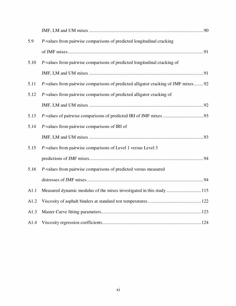
3.1 0.45 Power gradation charts of JMF mixes ....................................................................34

3.2 0.45 Power gradation curves of all JMF mixes...............................................................34

3.3 Shift in aggregate gradation after modification ..............................................................38

3.4 Air voids in test specimens ............................................................................................38

4.1 Master curves of JMF, LM and UM mixes.....................................................................51

4.2 Effect of air voids on dynamic modulus of replicates of JMF mixes...............................54

4.3 Dynamic modulus curves of JMF mixes ........................................................................56

4.4 Viscosity of asphalt binders versus temperature relationship ..........................................57

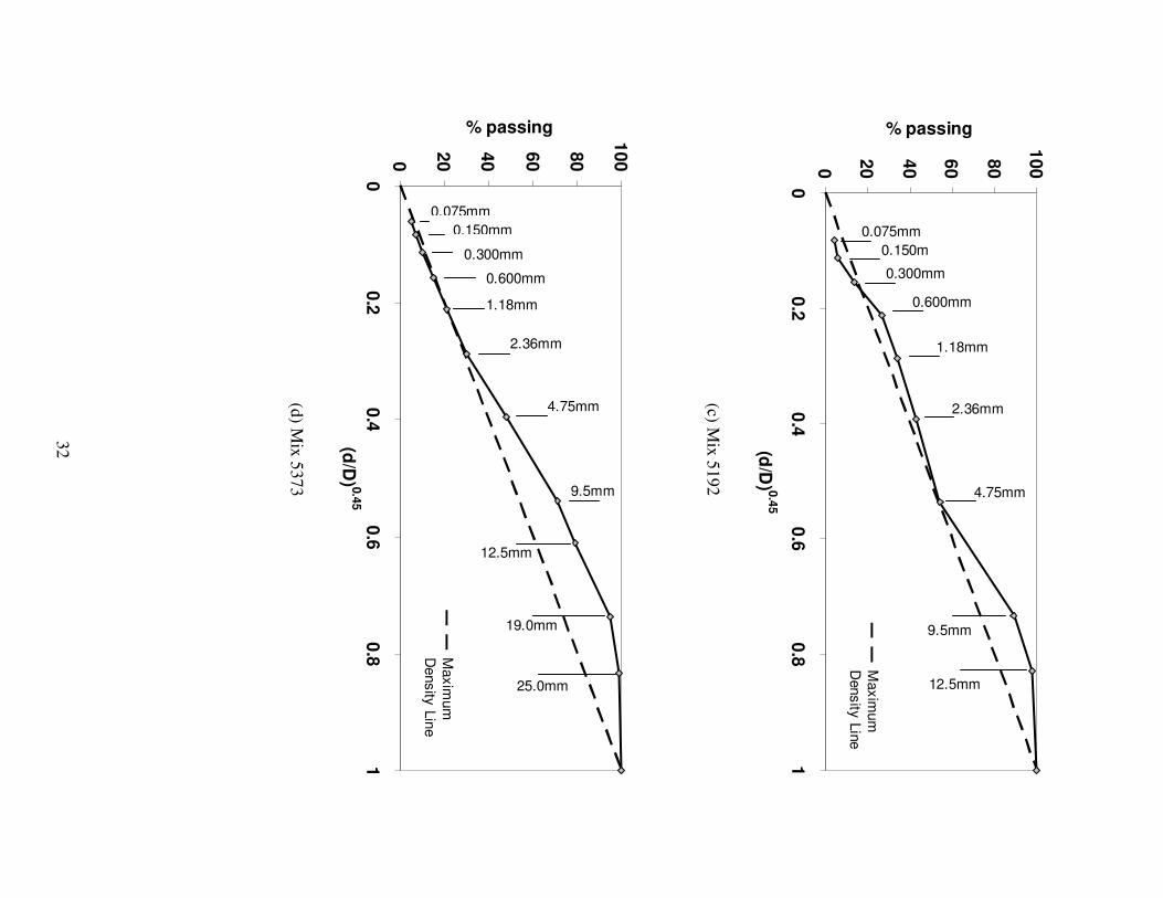
4.5 Dynamic modulus curves of JMF, LM and UM mixes at 4.4 °C ....................................60

4.6 Dynamic modulus curves of JMF, LM and UM mixes at 21.1 °C ..................................64



4.9 Dynamic modulus trend of the JMF mixes.....................................................................75

5.1 Predicted AC rutting over the design life .......................................................................95

5.2 Predicted versus measured asphalt concrete (AC) rutting ...............................................96

5.3 Predicted longitudinal cracking over the design life .......................................................97

5.4 Predicted versus measured longitudinal cracking ...........................................................98

5.5 Predicted alligator cracking over the design life .............................................................99

5.6 Predicted versus measured alligator cracking ...............................................................100

5.7 Predicted IRI over the design life.................................................................................101

5.8 Predicted versus measured IRI.....................................................................................102

xiii

A2.1 Typical raw dynamic modulus data measured at different temperatures and

frequencies ..................................................................................................................125

A2.2 Master curve constructed by shifting the curves in Fig. A1.1

with reference to 21.1°C ..............................................................................................125

A2.3 Master curve after sigmoidal curve fitting....................................................................126

A4.1 WSDOT pavement condition van ................................................................................134

A4.2 Arrangement of cameras and sensors ...........................................................................134

A4.3 Sample image of pavement condition survey ...............................................................135

1

CHAPTER ONE

INTRODUCTION

1.1 Background

Over the years, since the construction of the first pavement in the United States in 1870 at

Newark, New Jersey, pavement design has undergone many transformations. Especially, after

the release of the 1986 AASHTO Design Guide at which time the need for a mechanistic based

pavement design was recognized. Early pavement design methods were purely empirical and

aimed at determining the optimum thicknesses of pavement structural layers to provide adequate

strength and protection to the weak subgrade. With substantial changes in traffic volume and

loading conditions, the emphasis shifted away to pavement performance (ride quality). In the late

1950’s, construction of a series of test tracks was initiated, most importantly the AASHO Road

Test. Subsequently, the 1961 Interim Guide, the 1972 Interim Guide, the 1986 and 1993

AASHTO Guides were developed. The 1972 version was the first attempt towards the design of

overlays; the 1986 and 1993 versions of the AASHTO Guide addressed important issues like

better characterization of subgrade and unbound layers, drainage, environmental effects and

included reliability as a factor in the design. Even though empirical methods in the design were

accurate, they were valid only for the materials and environmental conditions upon which they

were developed.

The pavement community felt the need for a design method that will be valid over a

broad range of materials, environmental and loading conditions and takes in to account the

mechanical properties of pavement materials in the design. In 1988, the Strategic Highway

Research Program (SHRP) began with the primary goal of developing a rational mix design

2

procedure that will address the limitations of the existing design methods. Consequently, in 1993

the Superpave system emerged with the following elements: new grading system for asphalt

binders (performance graded (PG) grading system), guidelines for selection of aggregate, new

mix design and mixture analysis procedures. The Department of Transportation (DOT) in many

States in the country has adopted the Superpave method of design and many are in the process of

implementing it in the routine design procedure.

A major limitation of the Superpave method at the time of its release was the lack of a

strength test to evaluate the performance of compacted material. Instead, it relied mainly on

specifications for material selection and volumetric mix criteria to ensure satisfactory

performance. The industry realized the need for a strength test to ensure reliable mixture

performance over a wide range of traffic and climatic conditions. Subsequently, in 1996,

research began at the University of Maryland at College Park to identify and validate Simple

Performance Tests (SPT) for permanent deformation, fatigue cracking, and thermal cracking to

complement the Superpave volumetric mix design method. In 1999, the work was transferred to

NCHRP Project 9-19 “Superpave Support and Performance Models Management.” The research

team assessed existing test methods for measuring HMA response characteristics. The principal

evaluation criteria were (1) good correlation of the HMA response characteristics to actual field

performance; (2) reliability; (3) ease of use; and (4) reasonable equipment cost.

A comprehensive laboratory program was conducted in which material responses of

specimens prepared for 33 test method-test parameter combinations were measured. The

measured responses were statistically correlated with the performance data from accelerated

pavement testing projects, namely, WesTrack in Nevada, MnRoad in Minnesota, and FHWA

Accelerated Loading Facility (ALF) experiments. NCHRP Report 465 summarizes the

3

experimental and analytical work performed for this study, which recommends the following

SPT method-response parameter combinations selected for comprehensive field validation.

1. HMA Rutting (testing conducted at 37.8 to 54.4 °F)

- Dynamic complex modulus term, E*/sinφ, determined from the triaxial dynamic

modulus test

- Flow time, Ft, determined from the triaxial static creep test

- Flow number, Fn, determined from triaxial repeated load test

2. HMA Fatigue Cracking (testing conducted at 4.4 to 15.5 °C)

- Dynamic complex modulus, E*, determined from triaxial dynamic modulus test

3. HMA Low-Temperature Cracking (testing conducted at 0, -10, -20°C)

- Indirect tensile creep compliance, D(t), determined from indirect tensile creep test.

Another important step towards the development of a mechanistic based pavement design

procedure was the initiation of Project NCHRP 1-37A: Development of the 2002 Guide for

Design of New and Rehabilitated Pavement Structures. The project called for developing a guide

utilizing existing mechanistic-based models and databases, and reflecting current state-of-the-art

pavement design procedures. The guide was to address all new and rehabilitation design issues

and provide equitable design basis for all pavement types (NCHRP 1-37A). The NCHRP Project

1-37A concluded with the delivery of the 2002 Guide for Mechanistic-Empirical Design of New

and Rehabilitated Pavements Structures (MEPDG). The mechanistic-empirical numerical

models in the MEPDG were calibrated using performance data from the Long Term Pavement

Performance (LTPP) database. The numerical models require input data related to traffic,

4

climate, materials, and the proposed structure to predict damage accumulation over the service

life of the pavement. The MEPDG includes software, referred to as the Design Guide, for

analyzing existing pavements, identifying deficiencies in past designs, and predicting pavement

performance over time. The pavement community envisages MEPDG will be a major

improvement over the AASHTO 1993 guide in terms of achieving cost effective pavement

designs and rehabilitation strategies (AASHTO Memorandum, 2004), and SPT will play a major

role in quality control and selection of mixes with superior performance and improving the

reliability of performance prediction.

There is currently a national effort to implement performance tests as part of the

Superpave mix design for Hot-Mix-Asphalt (HMA), and to implement the 2002 Guide for

Mechanistic-Empirical Design of New and Rehabilitated Pavements Structures. Washington

State Department of Transportation (WSDOT) is in the process of implementing both Superpave

and MEPDG. It has created the need to investigate dynamic modulus of HMA mixes widely used

in the State of Washington and evaluate the MEPDG using local conditions.

1.2 Objectives of the Study

Following are the objectives of this study:

1. To investigate and develop a database of dynamic modulus of widely used

HMA mixes in the State of Washington,

2. To investigate the sensitivity of dynamic modulus to aggregate gradation,

3. To predict performance of the mixes using Design Guide (MEPDG software)

with Level 1 and Level 3 inputs, and the ability of dynamic modulus to

correlate with field performance, and

5

4. To evaluate the distress prediction accuracy of the MEPGD.

This study will help WSDOT to implement dynamic modulus as a performance test to

complement the volumetric mix design of HMA. The database will present representative

dynamic modulus values of the mixes investigated in this study, which can be used for

evaluating existing pavements, as inputs to the MEPDG for the design/analysis of flexible

pavements, and in future research.

1.3 Tasks

Following is the summary of the tasks carried out for the study:

� Selection of mixes; collection of materials and pavement performance data,

� Preparation of mixes,

� Specimen preparation for dynamic modulus tests; perform bulk specific gravity

tests to determine air voids in the specimens,

� Conduct dynamic modulus tests and develop master curves for all mixes,

� Analyze dynamic modulus data and verify results statistically,

� Predict distresses using Design Guide (MEPDG software),

� Evaluate distress prediction accuracy of the MEPDG by comparing predicted

distress data with measured distress data, and

� Create a database of dynamic modulus values of the mixes investigated, and a

database of parameters for determining dynamic modulus of the mixes

investigated at any temperature and frequency.

6

1.4 Organization of the Thesis

Chapter 2 focuses on dynamic modulus test and the salient features of the MEPDG. The

chapter also focuses on literature related to these topics.

Chapter 3 deals with the experimental part, which includes selection of mixes, mixture

volumetrics and material properties, mixture and specimen preparation, and the laboratory tests

performed. Tables and figures are presented at the end of the chapter.

Chapter 4 presents dynamic modulus data and master curves for the mixes investigated in

this study. Also presented are the results of the analysis of dynamic modulus data and Analysis

of Variance of the dynamic modulus data. Tables and figures are presented at the end of the

chapter.

Chapter 5 deals with the MEPDG Analysis, which includes a brief account of the distress

prediction mechanism incorporated in the MPEDG, the predicted performances (distresses) of

the mixes, results of the analysis of predicted distress data and statistical analyses of predicted

distress data. Tables and figures are presented at the end of the chapter.

Chapter 6 summarizes the conclusions derived from this study followed by Bibliography.

Appendix 1 presents the Dynamic Modulus Database.

Appendix 2 presents sample dynamic modulus master curves.

Appendix 3 explains terminologies related to Analysis of Variance (ANOVA).

Appendix 4 presents the methodology for distress data collection.

7

CHAPTER TWO

REVIEW OF DYNAMIC MODULUS TEST AND MEPDG

2.1 Dynamic Modulus Test

The relationship of stress versus strain of any linear viscoelastic material under

continuous sinusoidal loading is defined by a complex number called Complex Modulus denoted

by E*. The real part of complex modulus represents the elastic stiffness of the material; the

imaginary part represents the viscous behavior. Dynamic Modulus is the absolute value of

complex modulus denoted by |E*|. The stress-strain relationship of asphalt concrete, which is a

linear viscoelastic material, can be defined using dynamic modulus. Eq.2.1 shows the

mathematical form of dynamic modulus.

o

o

ε

σ*E = ............................................................................ (2.1)

where

σo = peak dynamic stress; and

εo = peak recoverable axial strain.

Dynamic modulus is determined by exerting sinusoidal (haversine) compressive load on

a cylindrical specimen of asphalt concrete measuring the applied stress and the resulting

recoverable strain. The test is performed at different temperatures and frequencies. Due to the

viscous nature of asphalt concrete, peak strain lags behind peak stress called as the phase angle

(φ), expressed in degrees. For pure elastic materials, φ equals zero; for pure viscous materials, φ

equals 90°. Mathematically,

8

(360)t

tφ

p

i ×= .................................................................... (2.2)

where

ti = time lag between a cycle of stress and strain (seconds); and

tp = time for a stress cycle (seconds).

It is important to understand that dynamic modulus is not a measure of strength; higher

dynamic modulus does not necessarily indicate higher strength, but only an indication that a

given applied stress produces lower strain in the mixture. The applications of dynamic modulus

and phase angle include characterization of asphalt concrete based on the susceptibility of a

mixture to distresses like permanent deformation and fatigue cracking, performance criteria in

asphalt concrete mixture design and key input parameter to the MEPDG.

2.1.1. Factors affecting dynamic modulus

Dynamic modulus of asphalt concrete is a function of material properties like aggregate

gradation, aggregate content, binder content, binder stiffness, and air voids; also, non-material

properties like test temperature and frequency, age and possibly specimen geometry (specimen

height-to-diameter ratio; MEPDG advocates using a height-to-diameter ratio of less than two)

affect dynamic modulus.

Tarefdar et al. (2006) studied the influence of aggregate gradation, asphalt type, asphalt

content, and air voids on dynamic modulus and rut potential. They investigated twelve “lab

mixes” and ten “plant mixes” from the Oklahoma Department of Transportation. They observed

no clear trend between modulus and asphalt content; modulus decreased with increase in air

9

voids. Rut potential increased with increase in asphalt content and with increase in air voids. The

mixes with coarser aggregate gradation produced the lowest rut potential; possibly the result of

better interlocking or higher stability provided by coarse aggregates. PG grade affected rutting

but not modulus at low to medium temperatures.

Vivek et al. (2006) evaluated the effect of height-to-diameter ratio on the accuracy of

measured dynamic modulus and the significance of end friction reducing (EFR) membranes on

dynamic modulus. Specimens with a diameter of 152 mm instead of the standard 102 mm

provided consistent results, especially if the ratio was less than two. EFR membranes increased

the accuracy of measured dynamic modulus.

Christopher et al. (2006) examined the effects of testing history and method of specimen

preparation, sawed/cored or compacted, on dynamic modulus. The two factors did not affect

dynamic modulus significantly. Mohammed et al. (2007) characterized thirteen plant-produced

HMA mixes based on dynamic modulus of the mixtures. Dynamic modulus was sensitive to

nominal maximum aggregate size (NMAS); recycled asphalt combined with larger size

aggregates exhibited higher dynamic modulus at high temperatures.

2.1.2 Predictive equations for dynamic modulus

Dynamic modulus test is laborious and not all situations demand measured dynamic

modulus values; for instance, trial designs or preliminary stages of a design. For such cases,

dynamic modulus can be predicted using regression models with the knowledge of certain

material properties. Several regression models are available for the prediction of dynamic

modulus; Witczak model and Hirsch model are the widely used predictive equations. HMA

10

volumetric properties and binder rheological properties are required for these models. The two

models are presented in the following sections.

Witczak Model

It is an empirical model developed based on the testing of 200 asphalt concrete mixtures.

It requires viscosity of asphalt binder and volumetric properties of asphalt-aggregate mixture to

predict dynamic modulus. It is capable of predicting |E*| over a range of temperatures, rates of

loading (frequency) and aging conditions. The model uses a symmetrical sigmoidal function,

presented in Eq.2.3:

( )ηg0.393532Log(f)0.313351Lo0.603313exp(1

)0.00547(ρ)0.000017(ρ)0.003958(ρ)0.0021(ρ3.871977

VV

0.802208V)0.058097(V

)0.002841(ρ)0.001767(ρ)0.02932(ρ1.249937logE

342

38384

abeff

beffa

42

200200

−−−+

+−+−

++

×−

−−+−=∗

.................................................................................... (2.3)

where

|E*| = dynamic modulus, 105 psi

η = viscosity of asphalt binder, 106 psi

f = frequency of loading, Hz

Va = air void content, %

Vbeff = effective asphalt binder content, % by volume

ρ34 = cumulative percent retained on the 19mm sieve

ρ38 = cumulative percent retained on the 9.5mm sieve

11

ρ4 = cumulative percent retained on the 4.76mm sieve

ρ200 = percent passing 0.075mm sieve

Hirsch model

Hirsch (1961) developed a model to calculate the modulus of elasticity of cement

concrete or mortar using aggregate modulus, mix proportions and elastic modulus of cement.

Christensen et al. (2003) extended this model for dynamic modulus of HMA. The model requires

|G*| of asphalt binder and volumetric properties of aggregate mixture to predict dynamic

modulus. They reported that the estimated standard error of the model was 41%. Eq.2.4 shows

the mathematical form of Hirsch model:

( )

+

−

−+

×+

−=

VFA|G*|3

VMA

4,200,000

100

VMA1

P1

10,000

VFAVMA|G*|3

100

VMA14,200,000P|E*|

binder

c

binderc

.................................................................................... (2.4)

where

( )

( )58.0

*

58.0

||3650

|*|320

+

+

=

VMA

VFAG

VMA

VFAG

Pc

|E*|mix = absolute value of mixture dynamic modulus

12

|G*|binder = absolute value of asphalt binder complex modulus

VMA = voids in mineral aggregate, %

VFA = voids filled with asphalt, %

Both models are based on limited data and require validation for other conditions.

Moreover, the models are reliable only up to a lower limit of |E*| below which testing is

required. Dongre et al. (2005) compared dynamic modulus of asphalt mixtures collected from

five pavement construction sites measured in the laboratory with the predicted values to evaluate

the prediction capacity of Witczak and Hirsch models. Both models were capable of predicting

dynamic modulus reasonably well; however, Hirsch model was valid over a wide range. It uses

|G*| data directly in the calculations reducing a source of error and is easier to use. They reported

that both models require corrections/refinements to improve accuracy.

Mohammed et al. (2006) evaluated Witczak’s model and Hirsch model by investigating

twenty-three plant-produced HMA mixtures in the Louisiana region. The two models predicted

dynamic modulus with reasonable reliability, which increased in Witczak’s model as the nominal

maximum aggregate size (NMAS) increased and increased in Hirsch model with decrease in

NMAS.

2.1.3 Dynamic modulus test implementation

Dynamic modulus test is still in the implementation stages in many states. Prior to

implementing the test, it is important to validate the test for local conditions, investigate dynamic

modulus of widely used HMA mixes in a particular region, and create a database. Shah et al.

(2005) measured dynamic modulus of eleven mixes commonly used in North Carolina. Dynamic

13

modulus was sensitive to binder content – higher sensitivity for modified binder. The study

provided feedback for implementing the test. Zhou et al. (2003) used field pavement conditions

to validate dynamic modulus test and the associated parameter, E*/sinφ, to support

implementation of the test in day-to-day Superpave design practice. Findings from this study

showed that dynamic modulus test is capable of distinguishing between good and poor mixtures.

2.2 Mechanistic Empirical Guide

The 2002 Guide for Mechanistic-Empirical Design of New and Rehabilitated Pavement

Structures (MEPDG) is the latest guide for new/rehabilitated flexible/rigid pavement design. All

design guides preceding the MEPDG employ empirical equations developed based on the

AASHO Road Test in the late 1950’s. Significant changes in construction materials, trucks and

truck volumes, and pavement construction techniques demanded the need for a mechanistic-

empirical design that will take in to account the mechanical properties of pavement materials,

and climatic effects; capable of predicting important types of distresses, and adapts to new

conditions. These factors laid the basis for the development of the MEPDG.

The MEPDG employs mechanistic models to predict structural responses that become

inputs to the empirical distress prediction models. The models were subjected to comprehensive

calibration routine until reasonable prediction of pavement performance was achieved. The

impact of climate and aging on material properties are incorporated in the design as biweekly

and monthly iterative predictions of pavement performance over the entire design life. The

complex models and design concepts come in a user-friendly software package called the

‘Design Guide’. Improvisations to the design procedure and Design Guide can be made over

14

time in a piecewise manner to any of the component models and incorporate them in the

procedure after recalibration and validation.

2.2.1 Hierarchical Inputs

An important aspect of the MEDPG is that it classifies the inputs, required for

design/analysis, in to three hierarchical levels – Level 1, Level 2, and Level 3. Level 1 inputs

provide the highest level of accuracy, appropriate for heavily trafficked pavements or where

safety and economic considerations for an early failure are a concern. Level 2 inputs provide an

intermediate level of accuracy, appropriate when resources or testing equipments are not

available. These are typically user-selected possibly from an agency database, derived from

limited testing program, or estimated through correlations. Level 3 inputs provide the lowest

level of accuracy, appropriate if the consequences of an early failure seems minimal. These are

typically user-selected from experience or typical averages for the region. The hierarchical input

system is upon the premise that design reliability increases when the level of engineering effort

expended for garnering inputs increases. This concept was validated only for the thermal fracture

module. The guide recommends initiatives to confirm this hypothesis for at least one major load-

related distress thereby illustrating that additional time and effort will result in a lower cost and

better performance of the pavement. Approximately 100 inputs are required for design/analysis

of pavements, which fall into three major categories: traffic, climate, and materials. Prediction

accuracy of the models, obviously, will not be sensitive to all inputs. Investigating the critical

inputs that affect the prediction accuracy of the models will help reduce the level of efforts

required to collect inputs.

15

Ali (2005) used laboratory measured material properties as inputs to investigate the

influence of material type on pavement performance predicted by the MEPDG. Dynamic

modulus estimated using predictive equations incorporated in the MEPDG differed substantially

from the measured values that resulted in underestimation of permanent deformation. The

models reflected sensitivity to HMA mix type, but not to variations in unbound material. They

recommended using nonlinear analysis to capture the real behavior of unbound materials, and

measured dynamic modulus (Level 1) rather than predicted values (Level 2).

Carvalho (2006) used Level 3 inputs to investigate the capacity of MEPDG to predict

pavement performance. Variation in thickness of HMA layer had significant impact on

prediction of performance. The influence of thickness of base layer on fatigue cracking and

permanent deformation was insubstantial. The study recommended the development of a

database of material property inputs for routine design applications.

Mohammad et al. (2006) investigated the sensitivity of dynamic modulus to predict

rutting using the Design Guide (MEPDG software). They reported that the rutting model in the

MEPDG requires more validation and calibration.

The MEPDG is versatile with provisions to choose combination of input levels, for

instance, HMA mix properties from Level 1, traffic data from Level 2 and subgrade properties

from Level 3. Nantung et al. (2005) reported that combinations of design input levels rather than

using a single design input level can yield results that are more rational. They found the default

traffic-load spectra (Level 3) in the Design Guide as too general lacking design accuracy and

recommended using at least a traffic input Level 2.

16

2.2.2 Structural Responses

The MEPDG predicts the following structural distresses in flexible pavement design and

analysis:

� Bottom-up fatigue (or alligator) cracking

� Surface-down fatigue (or longitudinal) cracking

� Permanent deformation (or rutting)

� Thermal cracking

� Fatigue in chemically stabilized layers (only considered in semi-rigid pavements)

2.2.3 Need for calibration/validation of the MEPDG

The MEPDG insists on calibrating/validating the mechanistic-empirical models to local

conditions because the distress mechanisms are too complex to develop a practical model and

developing empirical factors and subsequent calibration is necessary to obtain realistic

performance predictions. The rutting, fatigue cracking, and thermal cracking models in the

flexible design procedure have been calibrated using design inputs and performance data largely

from the LTPP database; although the database covers sections located throughout many parts of

North America it still may not be adequate for specific regions of the country. To address this

issue, the guide senses a need for more local or regional calibration/validation.

2.2.4 Implementation

The guide identifies various issues that need to be addressed prior to implementing the

MEPDG. The most important are to establish databases for inputs, to calibrate and validate

17

distress models for local conditions. The agency implementing the mechanistic-empirical design

procedure must address the implementation issues identified by the MEPDG.

Ceylan et al. (2005) investigated the sensitivity of design inputs pertaining to both rigid

and flexible pavements exhibiting particular sensitivity in Iowa using the Design Guide

(MEPDG software). The inputs for longitudinal and transverse cracking, rutting, and roughness

were categorized as extremely sensitive and sensitive to very sensitive and presented a strategic

plan for implementing MEPDG in Iowa.

Uzan et al (2005) carried out a sensitivity study to determine input variables for MEPDG

most important to Texas Department of Transportation (TxDOT). They found that the models

predicted rut depth adequately, slightly over-predicted alligator cracking, and inconsistent with

longitudinal cracking. The findings from this study supported the implementation of MEPDG

into TxDOT’s normal pavement design operations.

Gramajo (2005) used the Design Guide (MEPDG software) to predicted distress using

input data from actual pavement sections in the Commonwealth of Virginia. Predicted distresses

were higher than the field distresses. The study concluded that significant calibration and

validation is required before implementing MEPDG.

2.3 Summary

Dynamic modulus is a useful parameter for complementing the volumetric mixture

design and defining the stress-strain relationship of asphalt concrete. However, the test needs

calibration for local conditions before implementation in the routine design procedure. Dynamic

modulus can be predicted using Witczak’s model and Hirsch’s model. Hirsch’s model is

18

comparatively simple and the associated source of errors is relatively less; however, both models

need corrections/refinements for accurate prediction of dynamic modulus.

The 2002 Guide for Mechanistic-Empirical Design of New and Rehabilitated Pavement

Structures (MEPDG) is the recently developed guide for pavement design and a major step

towards mechanistic-based pavement design. It addresses the limitations of the existing

pavement design guides. The complex models and design concepts come in a user-friendly

software package called the Design Guide, which requires a comprehensive set of inputs for

predicting structural distresses. Depending upon the importance of the project, inputs could be

one or combination of the following: site-specific, from databases, based upon local conditions

or experience. The mechanistic-empirical models in the guide need calibration for local

conditions to obtain realistic performance predictions.

19

CHAPTER THREE

EXPERIMENT

The foremost step in this study was the selection of HMA mixes and collection of

materials followed by the experimental part, which comprised of dynamic modulus and dynamic

shear rheometer testing, and preparation of specimens for these tests. This chapter presents

details of the mixes selected for this study, properties of the materials, specimen preparation, and

the laboratory tests performed.

3.1 Mixes and Material Properties

Seven HMA mixes widely used in the State of Washington for the construction of

highways were selected for the study. For selecting the mixes, the criteria given below were

employed:

1. Mixes must possess different properties due to different aggregate source,

aggregate gradation, binder grade, binder content, or a combination of these,

2. Mixes used in the construction of highway sections with available

performance data, and

3. Availability of aggregates and binder.

Table 3.1 lists the HMA mixes selected for the study and the pavement sections

constructed using these mixes. The selected mixes, henceforth, are referred to as Job Mix

Formula (JMF). Table 3.2 summarizes the volumetrics of the JMF mixes, and asphalt binder

20

information. The VMA and VFA of the mixes satisfy the Superpave requirements: VMA – min.

13%, VFA – 65 to 75%. Various types of aggregates and aggregate structures were part of the

mixture design. Table 3.3 summarizes source, type, and other aggregate related properties. The

aggregates passed the Superpave requirements – flat and elongated particles (max. 10%) – single

fractured faces (min. 90%) – un-compacted voids in fine aggregate (min. 40%) – plastic fines in

graded aggregate (min. 40%).

3.1.1 Modified mixes

The amount of mineral filler (passing sieve #200) in a mix is critical during HMA plant

operations, which could influence the volumetrics of the mix significantly. In order to investigate

the sensitivity of dynamic modulus to variations in mineral filler, a ‘lower modified mix’,

designated as LM, and an ‘upper modified mix’, designated as UM, were prepared from each

JMF mix. In the LM mixes, percent-passing sieve #200 was reduced by 2%; in the UM mixes it

was increased by 2% (e.g. 7% becomes 5% in the LM mixes and 9% in the UM mixes). The

modifications to percent passing sieve #200 are based upon WSDOT tolerance limits

summarized in Table 3.4. Even though the tolerance limits include other sieve sizes and asphalt

content, because of lack of materials the focus was restricted to percent-passing sieve #200.

3.2 Gradation Charts

Gradation is an important property of aggregates that affects HMA properties like

stiffness, stability, and fatigue and frictional resistance. The best gradation is the one that gives

the densest packing of particles allowing sufficient voids for asphalt cement, and unfilled air

21

voids to avoid bleeding and/or rutting. Fuller and Thompson (1907) proposed an equation for

maximum density called as Fuller’s maximum density curve – Eq.3.1 below.

n

D

d100P

×= ................................................................... (3.1)

where,

d = diameter of the sieve size in question

D = maximum size of the aggregate

P = total percent passing or finer than the sieve

Federal Highway Administration (FHWA) used n=0.45 in Eq.3.1 and called it the 0.45

Power Gradation Chart. This chart is convenient for determining the maximum density line

(MDL) and for adjusting aggregate gradation. Maximum density line is a straight line joining the

origin with the percentage point of the maximum aggregate size. Fig.3.1 (a) through (g)

illustrates the 0.45 power gradation charts for the JMF mixes. The gradation curves of the JMF

mixes are close to MDL indicating that the aggregates are well graded.

Maximum density line is an ideal case, which might not always provide sufficient voids

for enough asphalt to achieve adequate durability. A densely packed aggregate might also lead to

a mixture more sensitive to even slight changes in asphalt. In such cases, a deviation from the

MDL creates sufficient voids in the mineral aggregate (VMA). In Fig.3.1, the gradations of some

of the mixes deviate from the MDL, which is a result of such adjustments. A combined gradation

chart, illustrated in Figure 3.2, compares the gradation curves of all JMF mixes.

Table 3.5 summarizes aggregate gradations of all mixes. Modifying the percent-passing

sieve #200 in the JMF mixes resulted in substantial reduction of mineral filler in the lower

22

modified mixes and vice versa in the upper modified mixes; approximately 25 to 40% by weight.

To balance the aggregate content in the mixes same as in the JMF mixes, rest of the sieve sizes

were proportionately adjusted. Table 3.6 summarizes the quantitative variations in the gradation

of all LM and UM mixes. Figure 3.3 (a) through (g) illustrates the effect of the modifications on

the gradation curves of LM and UM mixes. The gradation curves have shifted substantially in the

finer sieve sizes compared to the coarser ones.

3.3 Grouping of Mixes

In this study, twenty-one mixes were investigated, which include seven JMF, seven LM

and seven UM mixes. The mixes were grouped into seven Projects; each Project a combination

of JMF, LM and UM mixes. Hereinafter, the projects are referred to by the Mix ID’s listed in

Table 3.1. For instance, Project #5381 comprises JMF Mix #5381 and the two derived mixes –

LM and UM.

3.4 Laboratory Tests

The laboratory tests performed for the study include bulk specific gravity and dynamic

modulus test on HMA specimens, and dynamic shear rheometer test on asphalt binders.

Specimens for dynamic modulus tests, 100 mm in diameter and 150 mm in height, were cut and

cored from gyratory specimens 150 mm in diameter and 170 mm in height. Gyratory specimens

were compacted in the Superpave Gyratory Compactor (SGC) in accordance with AASHTO T

312. Bulk specific gravity, Gmb, of the specimens were measured in accordance with AASHTO T

166-05. Air voids in the gyratory and test specimens were determined using Eq.3.2. Table 3.7

summarizes Gmb, air voids, effective binder content, and unit weight of the test specimens.

23

Figure 3.4 illustrates the percent air voids in the test specimens. The target air voids in the test

specimens was 7±1%; however, in projects 5295 and 5627 the air voids in some specimens did

not meet this range, and replacement specimens were not possible because of lack of aggregates.

100G

G1AV(%)

mm

mb ×

−= .................................................. (3.2)

where,

AV = air voids in the specimen, %

Gmb = bulk specific gravity of the specimen

Gmm = maximum specific gravity of mixture

Dynamic modulus tests were performed in accordance with AASHTO TP 62-03, which

states that there is approximately 1.5 to 2.0 percent decrease in air voids when a specimen is cut-

cored from a gyratory specimen. To accommodate this variation, the target air voids in the

gyratory specimens was 9 ± 0.5% in order to achieve 7 ± 1.0 % air voids in the actual test

specimens. For each mix, two replicates were tested. The tests were performed at temperatures

4.4, 21.1, 37.8, and 54.4 °C, and frequencies 0.1, 0.5, 1, 5, 10, and 25 Hz. Prior to testing at each

temperature, the test specimens were conditioned in order to achieve uniform temperature. Three

equidistantly spaced LVDT’s were mounted on the test specimens to measure axial deformation

during the test. Table 3.8 summarizes the dynamic modulus test conditions in this study.

The purpose of a DSR test is to measure the complex shear modulus (G*) and phase

angle (δ) of asphalt binders. Typically, a specimen of asphalt binder is sheared between two

cylindrical plates; asphalt specimens are aged in the rolling thin film oven (RTFO) at 164 °C for

24

approximately 45 minutes prior to testing. The test is performed at different temperatures at a

constant angular frequency of 1.59 Hz. The diameter of the plates and the thickness of specimen

depend upon the test temperature. For all measurements taken at temperatures 46 °C and above,

a 25 mm diameter plate and a specimen height of 2 mm are used. For temperatures 37.8 °C and

lower, 8 mm diameter plate and a specimen height of 1 mm are used. Table 3.8 summarizes the

DSR test conditions in this study.

3.5 Summary

Twenty-one mixes were prepared and grouped in to seven projects. Each project was a

combination of seven JMF mixes, seven LM mixes and seven UM mixes. JMF mixes were the

ones selected for the study; LM mixes were prepared by decreasing the percent-passing sieve

#200 of the JMF mixes by 2%; increased by 2% in the UM mixes. Two replicates were prepared

for each mix. Test specimens (100 mm diameter by 150 mm height) for dynamic modulus tests

were cut-cored from gyratory specimens (150 mm diameter by 170 mm height). Target air voids

in the gyratory specimens were 9±0.5% to achieve 7±1% in the test specimens. Air voids in the

specimens were determined through bulk specific gravity tests. DSR tests were performed to

determine the G* and δ of the asphalt binders.

25

Table 3.1: Details of the pavement sections constructed using the mixes investigated in this

study

Mix

ID.

Pavement section Year SR Location/

County

Milepost

begin/end

Tonnage

(tons)

5381 Railroad Crossing to Canyon

Road, WA

1998 512 Tacoma/

Pierce

4.38/5.59 5695

5295 Thomas St. to N 152nd

St., WA

1998 99 Seattle/

King

34.85/35.46 30335

5192 MP 0.0 to King County

Line, WA

1997 99 Tacoma/

Pierce

0.50/1.05 2250

5373 V Mall Blvd. To Yak Riv Br.

& Wapato Cr. To Ahtanum

Cr., WA

1998 82 Yakima/

Yakima

36.31/38.05 12796

5627 Vic. Lind Coulee Bridge to

Vic. SR 90, WA

1999 17 Moses

lake/

Grant

43.00/45.22 15553

5364 Vancouver City Limits to S.E.

164th Ave., WA

1998 14 Vancouver/

Clark

6.58/7.93 31633

5408 SR 182 to SR 395, WA 1998 240 Richland/

Benton

37.78/40.18 30805

Table 3.2: Volumetrics of the selected mixes and asphalt binder properties

Mix ID

5381 5295 5192 5373 5627 5364 5408

NMAS, mm 12.5 12.5 12.5 19 19 12.5 12.5

MAS, mm 19 19 19 25 25 19 19

Asphalt content, % 5.7 5.3 5.1 5.4 4.5 5.6 5.4

Aggregate content, % 94.3 94.7 94.9 94.6 95.5 94.4 94.6

VFA, % 73 74.5 72.8 72.8 70.8 70.8 73.3

VMA, % 15.2 16.6 14.6 14.6 13.9 13.9 14.9

Gmm 2.492 2.486 2.483 2.551 2.616 2.502 2.523

Gmb 2.267 2.262 2.260 2.321 2.381 2.277 2.296

Asphalt

PG 58-22 70-22 64-22 70-28 64-28 58-22 64-28

Mixing temp, °C 136-141 154-159 153-158 160-171 160-168 136-141 157-162

Compaction temp, °C 133-138 145-150 142-147 138-149 138-149 133-138 146-151

Gb 1.0269 1.038 1.02 1.021 1.035 1.02 1.03

26

Table 3.3: Aggregate source, type, and properties

Mix ID

5381 5295 5192

5373 5627 5364 5408

Source B-333 B-335 B-335 E-141 GT-18 G-106 R-7

County Pierce King Pierce Yakima Grant Clark Benton

Type Vashon

recessional

outwash

gravels

Vashon

glacial

gravels

Vashon

glacial

gravels

Alluvial

gravels/

terrace

deposits

Outwash

flood

gravels

Outwash

flood

gravels

Alluvial

gravels

Gsb (coarse

aggregate)

2.681 2.703 2.65 2.712 2.783 2.718 2.643

Gsb (fine

aggregate)

2.646 2.625 2.626 2.609 2.76 2.598 2.705

Gsb (aggregate

blend) 2.653 2.646 2.631 2.653 2.771 2.603 2.699

Flat and elongated

particles (%)

0c

0b

0b

0b

3c

4.15a

n/a n/a

Single fractured

faces (%)

100b

100e

100f 100

f 94

b

98c

100e

100a

100b

99.5c

98e

91b

93c

96d

96b

95c

100g

Un-compacted

voids in fine

aggregate (%)

47.9 49 49 46.3 49 n/a n/a

Plastic fines in

graded aggregate

(%)

75 70 70 69 81 71 76

a (3/4" sieve); b (1/2” sieve); c (3/8” sieve); d (1/4” sieve); e (#4 sieve); f (#8 sieve); g(#10 sieve)

n/a – not available

27

Table 3.4: WSDOT tolerance limits for aggregate gradation and asphalt content

Sieve

(mm)

Tolerance limits

19 ± 6%

12.5 ± 6%

9.5 ± 6%

4.75 ± 5%

2.36 ± 4%

1.18 -

0.6 -

0.3 -

0.15 -

0.075 ± 2%

AC ± 0.5%

Table 3.5: Aggregate gradation of the mixes

Project Mix Sieve sizes (mm)

25 19 12.5 9.5 4.75 2.36 1.18 0.6 0.3 0.15 0.075 <0.075

JMF - - 6 9 30 18 12 7 6 4 3 5

5381 LM - - 6.1 9.2 30.6 18.4 12.2 7.1 6.1 4.1 3.1 3.1

UM - - 5.9 8.8 29.4 17.6 11.8 6.9 5.9 3.9 2.9 6.9

JMF - - 3 13 30 21 11 7 5 4 1.2 4.8

5295 LM - - 3.1 13.3 30.6 21.4 11.2 7.1 5.1 4.1 1.2 2.9

UM - - 2.9 12.7 29.4 20.6 10.8 6.9 4.9 3.9 1.2 3.2

JMF - - 2 9 35 11 9 7 13 8 2 5

5192 LM - - 2.2 8.5 35.1 11.7 9.1 73 13.5 7.5 1.6 5.2

UM - - 2.2 8.5 35.0 11.2 8.8 7.0 13.0 7.5 1.6 3.2

JMF 1 4 16 8 23 18 9 6 5 3 2 5

5373 LM 1.0 4.1 16.3 8.2 23.5 18.4 9.2 6.1 5.1 3.1 1.9 5.2

UM 1.0 3.9 15.7 7.8 22.5 17.6 8.8 5.9 4.9 2.9 1.0 4.1

JMF - 4 21 12 16 15 11 7 4 3 1 6

5627 LM - 4.1 21.4 12.2 16.3 15.3 11.2 7.1 4.1 3.1 1.0 3.2

UM - 3.9 20.6 11.8 15.7 14.7 10.8 6.9 3.9 2.9 1.0 7.8

JMF - - 6 16 23 17 14 7 6 3 3 5

5364 LM - - 6.1 16.3 23.5 17.3 14.3 7.1 6.1 3.1 3.1 3.1

UM - - 5.9 15.7 22.5 16.7 13.7 6.9 5.9 2.9 2.9 6.9

JMF - - 5 13 32 17 10 7 5 4 2 5

5408 LM - - 5.1 13.3 32.7 17.3 10.2 7.1 5.1 4.1 2.0 3.1

UM - - 4.9 12.7 31.4 16.7 9.8 6.9 4.9 3.9 2.0 6.9

JMF – Job Mix Formula; LM – lower modified mix; UM – upper modified mix

28

Table 3.6: Quantitative variation in gradation after modification

Project

5381 5295 5192

5373 5627 5364 5408 Size

(mm) LM UM LM UM LM UM LM UM LM UM LM UM LM UM

25 - - - - - - 2.0 -2.0 - - - - - -

19 - - - - - - 2.0 -2.0 -2.0 -2.0 - - - -

12.5 2.0 -2.0 2.0 -2.0 - 2.0 -2.0 -2.0 -2.0 -2.0 -2.0 2.0 -2.0

9.5 2.0 -2.0 2.0 -2.0 - 2.0 -2.0 -2.0 -2.0 -2.0 -2.0 2.0 -2.0

4.75 2.0 -2.0 2.0 -2.0 2.0 -2.0 2.0 -2.0 -2.0 -2.0 -2.0 -2.0 2.0 -2.0

2.36 2.0 -2.0 2.0 -2.0 2.0 -2.0 2.0 -2.0 -2.0 -2.0 -2.0 -2.0 2.0 -2.0

1.18 2.0 -2.0 2.0 -2.0 2.0 -2.0 2.0 -2.0 -2.0 -2.0 -2.0 -2.0 2.0 -2.0

0.6 2.0 -2.0 2.0 -2.0 2.0 -2.0 2.0 -2.0 -2.0 -2.0 -2.0 -2.0 2.0 -2.0

0.3 2.0 -2.0 2.0 -2.0 2.0 -2.0 2.0 -2.0 -2.0 -2.0 -2.0 -2.0 2.0 -2.0

0.15 2.0 -2.0 2.0 -2.0 2.0 -2.0 2.0 -2.0 -2.0 -2.0 -2.0 -2.0 2.0 -2.0

0.075 2.0 -2.0 2.0 -2.0 2.0 -2.0 2.0 -2.0 -2.0 -2.0 -2.0 -2.0 2.0 -2.0

< 75µ -38.8 37.3 -40.5 38.9 -25.5 24.5 -38.0 36.5 -32.0 30.7 -38.8 37.3 -38.8 37.3

LM – Lower modified mix; UM – Upper modified mix

All values are in percentage

29

Table 3.7: Properties of compacted test specimens

Mix Project

JMF1 JMF2 LM1 LM2 UM1 UM2

5381 AV 7.9 6.6 7.0 7.1 7.2 7.8

Gmb 2.296 2.324 2.316 2.315 2.313 2.298

Vbeff 12.7 12.9 12.9 12.8 12.8 12.8

Unit wt. 143 145 145 145 144 143

5295 AV 8.1 7.1 7.5 8.2 7.6 7.2

Gmb 2.282 2.31 2.299 2.282 2.297 2.306

Vbeff 11.7 11.8 11.7 11.7 11.7 11.8

Unit wt. 142 144 7.5 142 143 144

5192 AV 7 6.8 7.3 7.3 7.2 6.8

Gmb 2.31 2.314 2.301 2.301 2.305 2.315

Vbeff 11.6 11.6 11.5 11.5 11.5 11.6

Unit wt. 144 144 144 144 144 145

5373 AV 6.1 7.3 7.2 6.3 7.2 7.1

Gmb 2.393 2.363 2.364 2.389 2.328 2.37

Vbeff 12.7 12.5 12.5 12.6 12.5 12.5

Unit wt. 149 148 148 149 148 148

5627 AV 7.5 7.4 8.6 5.7 6.2 6

Gmb 2.421 2.423 2.39 2.466 2.455 2.459

Vbeff 10.5 10.5 10.4 10.7 10.7 10.7

Unit wt. 151.1 151.3 149.2 154.0 153.3 153.3

5364 AV 6.4 6.4 7.1 7.1 6.8 6.3

Gmb 2.343 2.343 3.324 2.325 2.333 2.343

Vbeff 12.2 12.2 12.2 12.2 12.2 12.2

Unit wt. 146 146 145 145 146 146

5408 AV 7.4 7.3 7.9 7.8 7.2 7.5

Gmb 2.335 2.339 2.324 2.326 2.342 2.334

Vbeff 12.0 12.0 12.0 12.0 12.1 12.0

Unit wt. 146 146 145 145 146 146

JMF1, JMF2 – field mix replicates; LM1, LM2 – lower modified mix replicates

UM1, UM2 – upper modified mix replicates

AV in percentage; Vbeff in percentage; Unit wt. in pcf

30

Table 3.8: Test conditions (temperature and frequency in the order of testing)

Mixture E* Temperature

° C 25 Hz 10 Hz 5 Hz 1 Hz 0.5 Hz 0.1 Hz

Binder G*

at 1.59 Hz

4.4 X X X X X X X

12.7 X

21.1 X X X X X X X

29.4 X

37.8 X X X X X X X

46.1 X

54.4 X X X X X X X

Table 3.9: G* and δ of the asphalt binders used in this study

Temperature (° C) Mix

-10 4.4 12.7 21.1 29.4 37.8 46.1 54.4

5381 G* - 43105 12524 3150.8 660.2 151.2 33.1 9.11

δ - 36.1 48.7 59.3 67.9 74.7 79.6 83.3

η 7.2x1010

9.51x107

5.51x106 5.05x10

5 7.27x10

4 1.42x10

4 3.7x10

3 1.19x10

3

5295 G* - 56547 17859 4885.3 1218.8 298.2 76.7 23.8

δ - 33.3 44 53.8 60.7 66.6 68.6 73.6

η 4.9x1010

1.45x108

1.10x107

1.20x106

1.94x105

4.03x104

1.08x104

3.45x103

5192 G* - 65321 22644 5052.8 1257.5 273.2 62.2 8.64

δ - 30.9 41.9 55.4 64.9 73.2 76.5 82.2

Η 6.4x1011

3.78x108

1.6x107

1.14x106

1.36x105

2.29x104

5.31x103

1.56x103

5373 G* - 18161 4905.4 1203.3 291.2 79.8 23.6 9.8

δ - 41.2 50.9 57.8 62.3 63.4 61.9 62

Η 1.8x109

1.43x107

1.66x106

2.57x105

5.45x104

1.42x104

4.58x103

1.71x103

5627 G* - 26387 7486.5 1839.8 422 110 29.3 8.74

δ - 41.8 52.2 61.4 67.5 73 76.4 80.2

η 9.1x109

2.94x107 2.4x10

6 2.87x10

5 5.03x10

4 1.14x10

4 3.32x10

3 1.16x10

3

5364 G* - 29451 9229.9 2437.5 568.1 131.3 28.4 8.9

δ - 38.2 47.7 57.1 65.2 71.7 75.9 80.8

Η 3.1x1010

6.04x107

4.03x106

4.11x105

6.4x104

1.33x104

3.61x103

1.2x103

5408 G* - 31156 9275.5 2360.3 546 131 28.6 8.72

δ - 38.3 48.1 57.5 65.7 72 76.7 81.5

η 3.2x1010

6.01x107

3.98x106

4.03x105

6.26x104

1.3x104

3.52x103

1.17x103

G* in kPa; δ in degrees; η in cP

31

0

20

40

60

80

100

0 0.2 0.4 0.6 0.8 1

(d/D)0.45

% p

as

sin

g

Maximum

Density Line

0.0

75m

m

0.1

50m

0.3

00m

m

0.6

00m

m

1.1

8m

m

2.3

6m

m

4.7

5m

m

9.5

mm

12.5

mm

(a) Mix 5381

0

20

40

60

80

100

0 0.2 0.4 0.6 0.8 1

(d/D)0.45

% p

as

sin

g

Maximum

Density Line

0.0

75m

m0.1

50m

m

0.3

00m

m

0.6

00m

m

1.1

8m

m

2.3

6m

m 4.7

5m

m

9.5

mm

12.5

mm

(b) Mix 5295

32

0

20

40

60

80

10

0

00

.20

.40

.60

.81

(d/D

) 0.4

5

% passing

Maxim

um

Density

Lin

e

0.075mm

0.150m

0.300mm

0.600mm

1.18mm

2.36mm

4.75mm

9.5mm

12.5mm

(c) Mix

5192

0

20

40

60

80

10

0

00

.20

.40

.60

.81

(d/D

) 0.4

5

% passing

Maxim

um

Density

Lin

e

0.075mm

0.150mm

0.300mm

0.600mm

1.18mm

2.36mm

4.75mm

9.5mm

12.5mm

19.0mm

25.0mm

(d) M

ix 5

373

33

0

20

40

60

80

100

0 0.2 0.4 0.6 0.8 1

(d/D)0.45

% p

as

sin

g

Maximum

Density Line

0.0

75m

m

0.1

50m

m

0.3

00m

m

0.6

00m

m

1.1

8m

m

2.3

6m

m 4.7

5m

m

9.5

mm

12.5

mm 19.0

mm

(e) Mix 5627

0

20

40

60

80

100

0 0.2 0.4 0.6 0.8 1

(d/D)0.45

% p

as

sin

g

Maximum

Density Line

0.0

75m

m

0.1

50m

m

0.3

00m

m

0.6

00m

m

1.1

8m

m

2.3

6m

m

4.7

5m

m

9.5

mm

12.5

mm

(f) Mix 5364

34

0

20

40

60

80

100

0 0.2 0.4 0.6 0.8 1

(d/D)0.45

% p

as

sin

g

Maximum

Density Line

0.0

75m

m

0.1

50m

m

0.3

00m

m

0.6

00m

m

1.1

8m

m

2.3

6m

m

4.7

5m

m

9.5

mm

12.5

mm

(g) Mix 5408

Figure 3.1: 0.45 Power gradation charts of JMF mixes

0

20

40

60

80

100

120

0 0.2 0.4 0.6 0.8 1 1.2

(d/D)0.45

% p

as

sin

g

5381

5295

5192

5373

5627

5364

5408

Figure 3.2: 0.45 Power gradation curves of all JMF mixes

35

1

10

100

0.01 0.1 1 10 100

Particle size, mm

% p

as

sin

g JMF

LM

UM

(a) Project 5381

1

10

100

0.01 0.1 1 10 100

Particle size, mm

% p

as

sin

g JMF

LM

UM

(b) Project 5295

36

1

10

100

0.01 0.1 1 10 100

Particle size, mm

% p

as

sin

g JMF

LM

UM

(c) Project 5192

1

10

100

0.01 0.1 1 10 100

Particle size, mm

% p

as

sin

g JMF

LM

UM

(d) Project 5373

37

1

10

100

0.01 0.1 1 10 100

Particle size, mm

% p

as

sin

g JMF

LM

UM

(e) Project 5627

1

10

100

0.01 0.1 1 10 100

Particle size, mm

% p

as

sin

g JMF

LM

UM

(f) Project 5364

38

1

10

100

0.01 0.1 1 10 100

Particle size, mm

% p

as

sin

g JMF

LM

UM

(g) Project 5408

Figure 3.3: Shift in aggregate gradation after modification

0

1

23

4

5

6

78

9

10


Mix

% a

ir-v

oid

s

5381

5295

5192

5373

5627

5364

5408

Figure 3.4: Air voids in test specimens (1 & 2 indicate replicates)

39

CHAPTER FOUR

ANALYSIS OF DYNAMIC MODULUS DATA

The step following the experimental part presented in Chapter 3 was the construction of

master curves for the mixes investigated using the raw dynamic modulus data. The master curves

were used for comparing the behavior of the mixes under load, and to investigate the sensitivity

of dynamic modulus to aggregate gradation; all inferences were validated statistically. Details of

the afore-mentioned tasks are presented in this chapter.

4.1 Dynamic Modulus Data and Master Curves

Dynamic modulus of the mixes investigated in this study is presented as a database in

Table A1.1 (a) through (g) Appendix 1. The database includes all mixes and replicates, and

projects. More details about the database and its applications are discussed in Appendix 1. One

of the limitations of dynamic modulus test is that it is impossible to simulate all possible field

conditions. Master curves are convenient tools for determining dynamic modulus at conditions

not possible in the laboratory, constructed by shifting dynamic modulus data collected at

different temperatures relative to time of loading, which is the inverse of frequency of loading.

4.1.1 Construction of Master Curves

There are different methods for constructing master curves. In this study, master curves

were constructed in accordance with the method recommended by MEPDG. Dynamic modulus

collected at 4.4, 37.7, and 54.4 °C were shifted relative to time of loading at 21.1 °C, which is

the reference temperature. Time of loading at the reference temperature was computed using

40

Eq.4.1, which requires viscosity of asphalt binder. Viscosities of the asphalt binders at different

temperatures and frequencies were computed using Eq.4.2, which is a correlation between

viscosity (η), complex shear modulus (G*), and phase angle (δ). As the usage of Eq.4.2 is

restricted to temperatures for which G* and δ data are known, viscosities at other temperatures

were determined using Eq.4.3. The procedure to compute regression parameters ‘A’ and ‘VTS’

in Eq.4.3 is explained in Chapter 2, Part 2 of the MEPDG. Table A1.2 Appendix 1 summarizes

the viscosities of the asphalt binders. The MEPDG states that viscosity of asphalt binders

approach a maximum value at very low temperatures, and must be restricted to 2.70 x 1010

Poise,

which was taken in to consideration for computing time of loading at the reference temperature.

( ) ( ) ( ) ( )]ηlogηc[logtlogrtlogrT−−= .............................. (4.1)

where,

tr = time of loading at the reference temperature, sec

t = time of loading, sec

η = viscosity at temperature of interest, cP

ηTr = viscosity at reference temperature, cP

4.8628*

sinδ

1

10

Gη

= .................................... .................. (4.2)

where

G* = binder complex shear modulus, Pa

41

δ = binder phase angle, degrees

η = viscosity, cP

( )RTlog VTSAloglogη += ............................................. (4.3)

where

η = viscosity, cP

TR = temperature in Rankine at which the viscosity was determined

A, VTS = regression parameters

rγlogtβe1

αχ|E*|log

++

+= .............................................. (4.4)

where,

E* = dynamic modulus, MPa

tr = time of loading at the reference temperature, sec (from Eq.4.2)

χ, α = fitting parameters; for a given set of data, χ represents the minimum value of log

(E*), and χ+α represents the maximum value of log (E*)

β, γ = parameters describing the shape of the sigmoidal function

Sigmoidal curve fitting

The shifted dynamic modulus data points take the shape of a sigmoidal curve defined by

the function Eq.4.4. Fitting a sigmoidal function to the shifted data points reduces scatter and

creates a smooth master curve. The fitting parameters in Eq.4.4 define two things: the shape of

the curve, and the time-temperature dependency of dynamic modulus. The ‘Solver’ function in

42

Excel was used for computing the fitting parameters. Firstly, χ and α were determined from the

dataset for which master curve is constructed; approximate values were assumed for parameters

β and γ, and the parameter ‘c’ in Eq.4.1. All five parameters were solved iteratively in Solver

until the sum of squared errors between measured and predicted dynamic modulus was close to

zero. Table A1.3, Appendix 1 summarizes the fitting parameters for the master curves of the

mixes investigated in this study, which can be used for determining dynamic modulus of a mix at

any temperature and frequency. A systematic procedure is presented in Section A1.4, Appendix

1.

Sample dynamic modulus curves illustrating the construction of master curves are

presented in Appendix 2. Fig.A2.1 is a typical dynamic modulus versus frequency plot; Fig.A2.2

illustrates the master curve before sigmoidal curve fitting; Fig.A2.3 illustrates the master curve

after fitting a sigmoidal function. Fig. 4.1 (a) through (g) illustrates the master curves of the

mixes after sigmoidal curve fitting.

4.1.2 Dynamic modulus at -10 °C

Dynamic modulus is a key input parameter to the MEPDG. The Design Guide (MEPDG

software) Version 1.000 mandates that dynamic modulus data for distress prediction should

consist at least one temperature in the range -17.7 to -6.7 °C. This temperature range is hard to

achieve in the laboratory using the Simple Performance Tester currently available at the

Washington Center for Asphalt Technology (WCAT); therefore, dynamic modulus values

corresponding to -10 °C were predicted using Eq.4.3 and the fitting parameters presented in

Table A1.2, Appendix 1.

43

4.2 Effect of air voids on dynamic modulus

Dynamic modulus of replicates of a mix could vary if there is significant variation in air

voids. Air voids in some replicates in this study differed significantly: Mix 5381 – 1.3%, Mix

5295 – 1%, Mix 5373 – 1.2%, but marginal in the other mixes. Fig.4.2 (a) through (g) compares

dynamic modulus curves of replicates of JMF mixes. The variation in dynamic modulus between

replicates is not significant in most cases, even in mixes 5381, 5295, and 5373. It appears that

variation in air voids had little effect on dynamic modulus of replicates although some cases

showed noticeable difference at high temperatures, which could be the result of variations in

experimental data.

4.3 Dynamic Modulus of JMF Mixes

Fig.4.3 (a) through (d) presents dynamic modulus curves of the JMF mixes at 4.4, 21.1,

37.8, and 54.4 °C. The curves are distinct at temperatures 37.8 and 54.4 °C, but not at 4.4 and

21.1 °C. This behavior could be attributed to aggregate interlocking and stiffness of asphalt. In

general, at low temperatures, stiffness of asphalt binder governs dynamic modulus of a mix while

at high temperatures it is governed by aggregate gradation and interlocking between particles.

Stiffness is a function of viscosity. Fig.4.4 illustrates viscosity versus temperature

relationship for the asphalt binders used in this study. At low temperatures, viscosities of the

asphalt binders show significant difference. As temperature increases, the difference becomes

less significant, exhibiting approximately same stiffness at high temperatures. Thereby, any

variation in dynamic modulus between the mixes at high temperatures (37.8 and 54.4 °C) must

be a result of aggregate gradation and interlocking between particles.

44

4.4 Sensitivity of Dynamic Modulus to Percent Passing Sieve No.200

Dynamic modulus curves of JMF, LM and UM mixes is illustrated in Fig.4.5 through 4.8.

The curves are distinct at 37.8 and 54.4 °C, but not at 4.4 and 21.1 °C, which is similar to the

behavior of the JMF mixes. The same phenomenon described in Section 4.3 is valid in this case

as well. However, in most cases, the LM and UM mixes do not follow a definite trend with the

JMF mixes. Thus, ±2% variations in percent-passing sieve #200 did not have significant effect

on dynamic modulus.

4.5 Statistical Analysis

The inferences in Section 4.4 and Section 4.5 were verified statistically. In general,

statistical analysis refers to a collection of methods used to process large amounts of data and

report overall trends. Some methods can be used to summarize or describe a collection of data

called as ‘descriptive statistics’. Some methods model the patterns in the data and draw

inferences about the process or population being studied called as ‘inferential statistics’. The

statistical analysis performed in this study falls in the latter type i.e., inferential statistics.

Appendix 3 presents some basic terminologies related to the statistical analysis performed in this

study.

4.5.1 Model

The objectives of the statistical analysis are to test if dynamic modulus of the JMF mixes

show significant difference, and to test if dynamic modulus of JMF, LM and UM mixes vary

significantly. A General Linear Model (GLM) was fitted to the dynamic modulus data and

analyzed using multi-factor analysis of variance (ANOVA) using the statistical software SAS

45

Version 9.1. The treatment factors were one or combinations of project, mix, temperature and

frequency – dynamic modulus was the response variable. Table 4.1 lists the levels of the

treatment factors. For all pairwise comparisons, Tukey’s Multiple Comparison Method was

employed. For Null hypothesis (H0), significance level of 0.05 was assumed. Section 4.6.3

presents the results of the analysis of the dynamic modulus data of the JMF mixes. Section 4.6.4

presents the results of the analysis of dynamic modulus data of JMF, LM and UM mixes.

4.5.2 JMF mixes

The dynamic modulus data of the JMF mixes was analyzed using Repeated Measures

ANOVA. Repeated measures ANOVA was used because the same specimen was tested at all

dynamic modulus test conditions – four temperatures and six frequencies, and a standard

ANOVA would fail to model the correlation between the repeated measures; here repeated

measures implies E* test conditions. The treatment factors were project, mix, temperature, and

frequency. To test null hypothesis (i.e., there is no significant difference in dynamic modulus of

the seven JMF mixes), p-values from Tukey’s pairwise comparisons of the JMF mixes were

compared with the significance level 0.05. Table 4.2 summarizes the p-values; majority is

smaller than 0.05 indicating that the JMF mixes are significantly different. In addition, the Type I

p-value is 0.0015, which is an overall indication that significant difference in dynamic modulus

exists among the mixes. This supports Section 4.3, wherein it was shown that dynamic modulus

of the JMF mixes exhibited variation. Fig.4.10 is a plot of the mean dynamic modulus of the

seven mixes. Dynamic modulus of the JMF mixes follows the trend: 5364 < 5373 < 5408 < 5381

< 5627 < 5295 < 5192.

46

4.5.3 JMF, LM and UM Mixes

To test if dynamic modulus of JMF, LM and UM mixes vary significantly, dynamic

modulus data of JMF, LM and UM mixes of each project were analyzed separately using

Repeated Measures ANOVA. Table 4.3 summarizes the p-values from Tukey’s pairwise

comparisons of the three mixes; majority is larger than 0.05 indicating that dynamic modulus of

the three mixes is not different. In addition, the Type I p-values of all the projects, except 5381

and 5364, are larger than 0.05, which also indicates that significant difference does not exist.

This supports the inferences presented in Section 4.4, wherein it was shown that dynamic

modulus was not sensitive to ±2% variation in percent-passing sieve #200.

4.6 Summary

Dynamic modulus of the JMF mixes varied significantly at high temperatures compared

to low temperatures. Conversely, dynamic modulus of JMF, LM and UM mixes did not exhibit

significant variation; also, LM and UM mixes did not follow a definite trend with JMF mixes.

Thus, the behavior of the seven HMA mixes selected for this study was different under load, and

varying percent-passing sieve #200 by ±2% did not have significant effect on dynamic modulus.

Results from the Analysis of Variance of the dynamic modulus data supported these inferences.

In some projects, air voids of replicates varied by approximately 1%, which did not have

significant effect on dynamic modulus of replicates.

47

Table 4.1: Levels of treatment factors for ANOVA of dynamic modulus data

Levels

Block (Project) 7 5381, 5295, 5192, 5373, 5627, 5364, 5408

Mix 3 JMF, lower modified, upper modified

Temperature, ° C 4 4.4, 21.1, 37.8, 54.4

Frequency, Hz 6 25, 10, 5, 1, 0.5, 0.1

Table 4.2: P-values from pairwise comparisons of dynamic modulus of JMF mixes

Project 5381 5295 5192 5373 5637 5364 5408

5381 - 0.9295 0.4391 0.0559 0.9865 0.0341 0.1575

5295 - 0.9205 0.0174 0.9999 0.0111 0.046 5192 - 0.0059 0.7975 0.0039 0.0141

5373 - 0.0245 0.9991 0.9672

5627 - 0.0154 0.0665

5364 - 0.836

5408 -

Table 4.3: P-values from pairwise comparisons of JMF, LM and UM mixes

Project Mix UM LM Type I

5381 JMF 0.0196 0.0674 0.0215

LM 0.2162 -

5295 JMF 0.4824 0.6572 0.2259

LM 0.2087 -

5192 JMF 0.9999 0.8769 0.8514

LM 0.872 -

5373 JMF 0.1732 0.5857 0.1892

LM 0.451 -

5627 JMF 0.719 0.4825 0.5028

LM 0.8817 -

5364 JMF 0.4056 0.0026 0.0016 LM 0.0018 -

5408 JMF 0.8616 0.2081 0.2088

LM 0.3342 -

48

1

10

100

1000

10000

100000

0.00001 0.001 0.1 10 1000 100000

Frequency, Hz

Dy

na

mic

Mo

du

lus

, M

Pa

JMF1

JMF2

LM1

LM2

UM1

UM2

(a) 5381

1

10

100

1000

10000

100000

0.00001 0.001 0.1 10 1000 100000

Frequency, Hz

Dy

na

mic

Mo

du

lus

, M

Pa

JMF1

JMF2

LM1

LM2

UM1

UM2

(b) 5295

49

1

10

100

1000

10000

100000

0.00001 0.001 0.1 10 1000 100000

Frequency, Hz

Dy

na

mic

Mo

du

lus

, M

Pa

JMF1

JMF2

LM1

LM2

UM1

UM2

(c) 5192

1

10

100

1000

10000

100000

0.00001 0.001 0.1 10 1000 100000

Frequency, Hz

Dy

na

mic

Mo

du

lus

, M

Pa

JMF1

JMF2

LM1

LM2

UM1

UM2

(d) 5373

50

1

10

100

1000

10000

100000

0.0001 0.01 1 100 10000

Frequency, Hz

Dy

na

mic

Mo

du

lus

, M

Pa

JMF1

JMF2

LM1

LM2

UM1

UM2

(e) 5627

1

10

100

1000

10000

100000

0.0001 0.01 1 100 10000

Frequency, Hz

Dy

na

mic

Mo

du

lus

, M

Pa

JMF1

JMF2

LM1

LM2

UM1

UM2

(f) 5364

51

1

10

100

1000

10000

100000

0.0001 0.01 1 100 10000

Frequency, Hz

Dy

na

mic

Mo

du

lus

, M

Pa

JMF1

JMF2

LM1

LM2

UM1

UM2

(g) 5408

Figure 4.1: Master curves of JMF, LM and UM mixes

1

10

100

1000

10000

100000

0 1 10 100

Frequency, Hz

Dy

na

mic

mo

du

lus

, M

Pa

JMF1 4.4 °C

JMF2 4.4 °C

JMF1 21.1 °C

JMF2 21.1 °C

JMF1 37.8 °C

JMF2 37.8 °C

JMF1 54.4 °C

JMF2 54.4 °C

(a) Project 5381; JMF1 – 7.9% AV, JMF2 – 6.6% AV

52

1

10

100

1000

10000

100000

0.1 1 10 100

Frequency, Hz

Dy

na

mic

mo

du

lus

, M

Pa

JMF1 4.4 °C

JMF2 4.4 °C

JMF1 21.1 °C

JMF2 21.1 °C

JMF1 37.8 °C

JMF2 37.8 °C

JMF1 54.4 °C

JMF2 54.4 °C

(b) Project 5295; JMF1 – 8.1% AV, JMF2 – 7.1% AV

1

10

100

1000

10000

100000

0.1 1 10 100

Frequency, Hz

Dy

na

mic

mo

du

lus

, M

Pa

JMF1 4.4 °C

JMF2 4.4 °C

JMF1 21.1 °C

JMF2 21.1 °C

JMF1 37.8 °C

JMF2 37.8 °C

JMF1 54.4 °C

JMF2 54.4 °C

(c) Project 5192; JMF1 – 7.0% AV, JMF2 – 6.8% AV

53

1

10

100

1000

10000

100000

0.1 1 10 100

Frequency, Hz

Dy

na

mic

mo

du

lus

, M

Pa

JMF1 4.4 °C

JMF2 4.4 °C

JMF1 21.1 °C

JMF2 21.1 °C

JMF1 37.8 °C

JMF2 37.8 °C

JMF1 54.4 °C

JMF2 54.4 °C

(d) Project 5373; JMF1 – 6.1% AV, JMF2 – 7.3% AV

1

10

100

1000

10000

100000

0.1 1 10 100

Frequency, Hz

Dy

na

mic

mo

du

lus

, M

Pa

JMF1 4.4 °C

JMF2 4.4 °C

JMF1 21.1 °C

JMF2 21.1 °C

JMF1 37.8 °C

JMF2 37.8 °C

JMF1 54.4 °C

JMF2 54.4 °C

(e) Project 5627; JMF1 – 7.5% AV, JMF2 – 7.4% AV

54

1

10

100

1000

10000

100000

0.1 1 10 100

Frequency, Hz

Dy

na

mic

mo

du

lus

, M

Pa

JMF1 4.4 °C

JMF2 4.4 °C

JMF1 21.1 °C

JMF2 21.1 °C

JMF1 37.8 °C

JMF2 37.8 °C

JMF1 54.4 °C

JMF2 54.4 °C

(f) Project 5364; JMF1 – 6.4% AV, JMF2 – 6.4% AV

1

10

100

1000

10000

100000

0.1 1 10 100

Frequency, Hz

Dy

na

mic

mo

du

lus

, M

Pa

JMF1 4.4 °C

JMF2 4.4 °C

JMF1 21.1 °C

JMF2 21.1 °C

JMF1 37.8 °C

JMF2 37.8 °C

JMF1 54.4 °C

JMF2 54.4 °C

(g) Project 5408; JMF1 – 7.4% AV, JMF2 – 7.3% AV

Figure 4.2: Effect of air voids on dynamic modulus of replicates of JMF mixes

55

1

10

100

1000

10000

100000

0.1 1 10 100

Frequency, Hz

Dy

na

mic

Mo

du

lus

, M

Pa

5381

5295

5192

5373

5627

5364

5408

(a) 4.4 °C

1

10

100

1000

10000

0.1 1 10 100

Frequency, Hz

Dy

na

mic

Mo

du

lus

, M

Pa

5381

5295

5192

5373

5627

5364

5408

(b) 21.1 °C

56

1

10

100

1000

10000

0.1 1 10 100

Frequency, Hz

Dy

na

mic

Mo

du

lus

, M

Pa

5381

5295

5192

5373

5627

5364

5408

(c) 37.8 °C

1

10

100

1000

10000

0.1 1 10 100

Frequency, Hz

Dy

na

mic

Mo

du

lus

, M

Pa

5381

5295

5192

5373

5627

5364

5408

(d) 54.4 °C

Figure 4.3: Dynamic modulus curves of JMF mixes

57

1.E+03

1.E+04

1.E+05

1.E+06

1.E+07

1.E+08

1.E+09

4.4 12.7 21.1 29.4 37.8 46.1 54.4

Temperature, deg

Vis

co

sit

y, c

P58-22 (5381) 70-22 (5295)64-22 (5192) 70-28 (5373)64-28 (5627) 58-22 (5364)64-28 (5408)

Figure 4.4: Viscosity of asphalt binders versus temperature relationship

10

100

1000

10000

100000

0 1 10 100

Frequency, Hz

Dy

na

mic

mo

du

lus

, M

Pa

JMF1

JMF1

LM1

LM2

UM1

UM2

(a) 5381

58

10

100

1000

10000

100000

0 1 10 100

Frequency, Hz

Dy

na

mic

mo

du

lus

, M

Pa

JMF1

JMF2

LM1

LM2

UM1

UM2

(b) 5295

10

100

1000

10000

100000

0.1 1 10 100

Frequency, Hz

Dy

na

mic

mo

du

lus

, M

Pa

JMF1

JMF2

LM1

LM2

UM1

UM2

(c) 5192

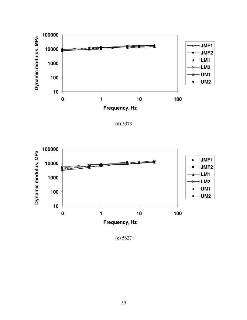
59

10

100

1000

10000

100000

0 1 10 100

Frequency, Hz

Dy

na

mic

mo

du

lus

, M

Pa

JMF1

JMF2

LM1

LM2

UM1

UM2

(d) 5373

10

100

1000

10000

100000

0 1 10 100

Frequency, Hz

Dy

na

mic

mo

du

lus

, M

Pa

JMF1

JMF2

LM1

LM2

UM1

UM2

(e) 5627

60

10

100

1000

10000

100000

0 1 10 100

Frequency, Hz

Dy

na

mic

mo

du

lus

, M

Pa

JMF1

JMF2

LM1

LM2

UM1

UM2

(f) 5364

10

100

1000

10000

100000

0 1 10 100

Frequency, Hz

Dy

na

mic

mo

du

lus

, M

Pa

JMF1

JMF2

LM1

LM2

UM1

UM2

(g) 5408

Figure 4.5: Dynamic modulus curves of JMF, LM and UM mixes at 4.4 °C

61

10

100

1000

10000

0.1 1 10 100

Frequency, Hz

Dy

na

mic

mo

du

lus

, M

Pa

JMF1

JMF2

LM1

LM2

UM1

UM2

(a) 5381

10

100

1000

10000

0.1 1 10 100

Frequency, Hz

Dy

na

mic

mo

du

lus

, M

Pa

JMF1

JMF2

LM1

LM2

UM1

UM2

(b) 5295

62

10

100

1000

10000

0.1 1 10 100

Frequency, Hz

Dy

na

mic

mo

du

lus

, M

Pa

JMF1

JMF2

LM1

LM2

UM1

UM2

(c) 5192

10

100

1000

10000

0.1 1 10 100

Frequency, Hz

Dy

na

mic

mo

du

lus

, M

Pa

JMF1

JMF2

LM1

LM2

UM1

UM2

(d) 5373

63

10

100

1000

10000

0.1 1 10 100

Frequency, Hz

Dy

na

mic

mo

du

lus

, M

Pa

JMF1

JMF2

LM1

LM2

UM1

UM2

(e) 5627

10

100

1000

10000

0.1 1 10 100

Frequency, Hz

Dy

na

mic

mo

du

lus

, M

Pa

JMF1

JMF2

LM1

LM2

UM1

UM2

(f) 5364

64

10

100

1000

10000

0.1 1 10 100

Frequency, Hz

Dy

na

mic

mo

du

lus

, M

Pa

JMF1

JMF2

LM1

LM2

UM1

UM2

(g) 5408


10

100

1000

10000

0 1 10 100

Frequency, Hz

Dy

na

mic

mo

du

lus

, M

Pa

JMF1

JMF2

LM1

LM2

UM1

UM2

(a) 5381

65

10

100

1000

10000

0.1 1 10 100

Frequency, Hz

Dy

na

mic

mo

du

lus

, M

Pa

JMF1

JMF2

LM1

LM2

UM1

UM2

(b) 5295

10

100

1000

10000

0 1 10 100

Frequency, Hz

Dy

na

mic

mo

du

lus

, M

Pa

JMF1

JMF2

LM1

LM2

UM1

UM2

(c) 5192

66

10

100

1000

10000

0 1 10 100

Frequency, Hz

Dy

na

mic

mo

du

lus

, M

Pa

JMF1

JMF2

LM1

LM2

UM1

UM2

(d) 5373

10

100

1000

10000

0 1 10 100

Frequency, Hz

Dy

na

mic

mo

du

lus

, M

Pa

JMF1

JMF2

LM1

LM2

UM1

UM2

(e) 5627

67

10

100

1000

10000

0 1 10 100

Frequency, Hz

Dy

na

mic

mo

du

lus

, M

Pa

JMF1

JMF2

LM1

LM2

UM1

UM2

(f) 5364

10

100

1000

10000

0 1 10 100

Frequency, Hz

Dy

na

mic

mo

du

lus

, M

Pa

JMF1

JMF2

LM1

LM2

UM1

UM2

(g) 5408


68

10

100

1000

10000

0.1 1 10 100

Frequency, Hz

Dy

na

mic

mo

du

lus

, M

Pa

JMF1

JMF2

LM1

LM2

UM1

UM2

(a) 5381

10

100

1000

10000

0.1 1 10 100

Frequency, Hz

Dy

na

mic

mo

du

lus

, M

Pa

JMF1

JMF2

LM1

LM2

UM1

UM2

(b) 5295

69

10

100

1000

10000

0.1 1 10 100

Frequency, Hz

Dy

na

mic

mo

du

lus

, M

Pa

JMF1

JMF2

LM1

LM2

UM1

UM2

(c) 5192

10

100

1000

10000

0.1 1 10 100

Frequency, Hz

Dy

na

mic

mo

du

lus

, M

Pa

JMF1

JMF2

LM1

LM2

UM1

UM2

(d) 5373

70

10

100

1000

10000

0.1 1 10 100

Frequency, Hz

Dy

na

mic

mo

du

lus

, M

Pa

JMF1

JMF2

LM1

LM2

UM1

UM2

(e) 5627

10

100

1000

0.1 1 10 100

Frequency, Hz

Dy

na

mic

mo

du

lus

, M

Pa

JMF1

JMF2

LM1

LM2

UM1

UM2

(f) 5364

71

10

100

1000

0.1 1 10 100

Frequency, Hz

Dy

na

mic

mo

du

lus

, M

Pa

JMF1

JMF2

LM1

LM2

UM1

UM2

(g) 5408


0

1000

2000

3000

4000

5000

6000

5381 5295 5192 5373 5627 5364 5408

Project

Av

era

ge

E*,

MP

a

Figure 4.9: Dynamic modulus trend of the JMF mixes

72

CHAPTER FIVE

MEPDG ANALYSIS

One of the objectives of this study was to evaluate the MEPDG, which was the next step

in this study. This was done by predicting the performance of the mixes investigated in this study

and comparing them with the measured (field) distresses. Performance of the mixes i.e. distresses

were predicted using Design Guide (MEPDG software). A combination of site-specific data and

default data in the software were used as inputs to the Design Guide. Details of the evaluation of

the MEPDG are presented in this chapter.

5.1 Distress Prediction Mechanism in the MEPDG

The mechanistic models in the MEPDG divide the design life in to shorter analysis

periods or increments beginning with the traffic-opening month. All factors – traffic level,

asphalt concrete modulus, base-, subbase-, and subgrade modulus – that affect pavement

responses and distresses remain constant within each increment. For each increment, critical

stresses and strains are determined for all distress types and converted in to incremental

distresses. The incremental distress could be either in absolute terms or in terms of a ‘damage

index’, which is a mechanistic parameter representing the load-associated damage within the

pavement structure. Cracking distresses (longitudinal cracking, alligator cracking, and thermal

cracking) are predicted in terms of damage index, smaller the index (e.g., 0.0001) less significant

will be the cracking and vice-versa. At the end of the analysis, damage is summed – calibrated

models relate the cumulative damage to observable distresses. Rutting is predicted in absolute

73

terms allowing direct accumulation of the computed incremental distress for the entire design

life.

5.2 Analysis

The objectives of the MEPDG analysis are to predict the performance of the mixes

investigated in this study, to perform a simple evaluation of the distress prediction accuracy and

to investigate the ability of dynamic modulus to correlate with distresses; however, calibrating

the MEPDG prediction models is not in the scope of this study.

Design Guide Version 1.000 was used for predicting distresses. It gives the user the

option to choose either the NCHRP 1-37A viscosity based model or the NCHRP 1-40D G*

based model. The viscosity-based model was opted because the G* based model is yet to be

calibrated nationally. Taking into consideration the fact that the pavement sections constructed

using the selected mixes are overlays, AC over AC type of rehabilitation design was opted in all

cases.

The MEPDG analysis was divided into two parts: Level 1 Analysis and Level 3 Analysis.

In Level 1 Analysis, E*, G* and δ were used as Level 1 material inputs. In Level 3 Analysis,

aggregate gradation and asphalt PG grade were used as Level 3 material inputs. All other inputs

– traffic, climatic and materials – were a combination of site-specific data and default values in

the software, which remained constant in both levels of analysis. The design life for all cases was

taken as 20 years. The following distresses were predicted:

� Longitudinal cracking

� Alligator cracking

� Rutting

74

� International Roughness Index (IRI)

5.2.1 Inputs

Traffic data for the analyses were a combination of site-specific data, and default data in

the Design Guide; Table 5.1 summarizes the site-specific traffic data. Inputs to the Enhanced

Integrated Climatic Model (EICM) were the climatic files incorporated in the Design Guide –

climatic data either from the nearest weather station or from a combination of weather stations

proximate to the location of the pavement section; Table 5.2 lists the weather station locations. In

all cases, the water table was assumed 15m below ground level. Table 5.3 summarizes the details

of the pavement structural layers used in the analysis. A cement-stabilized base layer replaced

the PCC layer in projects 5295, 5192 and 5364 because of insufficient data. For all unbound

layers – granular bases, cement stabilized bases, and subgrade (appropriate to the AASHTO soil

type used in the field) – default material properties in the Design Guide were used and were

assumed ‘compacted’. The existing asphalt layer (the layer below the overlay) in all cases was

Class-A Type Asphalt Concrete; the properties are summarized in Table 5.4.

5.3 Field Performance Data

The performance of the pavement sections constructed using the mixes investigated in

this study were obtained from recent distress data collection performed by WSDOT. Table 5.5

presents the month and year distress measurements were made on the pavement sections, and

average distress values.

Typically, distress data is collected using a Pavement Condition Van (PCV), which is

operated by a two-person team driving at the posted speed limit. The PCV is equipped with

75

cameras that capture different sections of the surface of the pavement that are used for

quantifying surface distresses (cracking, patching, etc.); images are captured each 25 feet. To

measure roadway profile, rutting/wear, and faulting laser sensors are mounted on the front and

rear of the PCV. The data recorded by these sensors are processed using computer programs to

determine roughness, faulting, and maximum wheel path wear depth. The digital images are

analyzed using specially developed computer program and viewed one by one for a variety of

distresses (cracking, patching, spalling, etc.), which is called as pavement distress rating, usually

done in 0.10 miles increments. After completing the pavement distress rating for a pavement

section, the length and type of distress are summed. The data presented in Table 5.5 were

collected in this manner. More information on distress data collection is given in Appendix 4.

5.4 Results

The output generated by the Design Guide is a comprehensive file that contains, along

with other important information, predicted incremental distress values for all distress types on a

monthly basis over the entire design life. The condition of a pavement at any point during the

design life is read from the output file by looking at the appropriate month and year. Table 5.6

presents the predicted performance of the mixes investigated in this study, extracted from the

output file, corresponding to the month and year of distress data collection. For instance, the

pavement section constructed using mix#5381 was opened to traffic in August 1998; the recent

distress data collection was made in September 2006. Thereby, the predicted distress values for

Mix #5381, presented in Table 5.6, correspond to September 2006 in the output file.

The type of distress data (incremental or extracted) used in the analysis depended upon

the objective. For comparing the performance of the mixes, incremental distress data were used;

76

to investigate if dynamic modulus correlated with distresses, distress values at the end of the

design life were used; and to evaluate the prediction accuracy of the Design Guide, data

presented in Table 5.5, and Table 5.6 were used. In all cases, each distress type was analyzed

separately and the inferences were validated statistically. Following are the cases analyzed

statistically for validating the inferences derived from distress data analysis:

1. “Comparison of the performance of the mixes” – the distresses of the seven JMF

mixes were analyzed using Two-Way ANOVA with ‘Project’ and ‘input level’ as

the treatment factors; input level implies Level 1 Analysis or Level 3 Analysis.

2. “Did variation in percent passing sieve #200 affect the performance of the

mixes?” – The predicted distresses of JMF, LM and UM mixes were analyzed

using a Two-Way ANOVA with ‘mix’ and ‘input level’ as the treatment factors;

the distress data of the three mixes in each project were analyzed separately.

3. “How accurate is the MEPDG in predicting distress?” – To test if the predicted

distresses differed from the measured distresses, and if Level 1 predictions are

significantly different from Level 3 Analysis predictions a One-Way ANOVA

was run with ‘level’ (Level 1, Level 3, and Field) as the treatment factor. For all

pairwise comparisons, Tukey’s method was employed assuming a significance

level of 0.05.

In all three statistical analyses, the data presented in Table 5.5 (measured) and Table 5.6

(predicted) were used. The results of the MEPDG analysis are presented in the following

sections – each distress type separately.

77

5.4.1 Predicted AC rutting

Rutting is a plastic/viscoelastic deformation that manifests in the form of surface

depression in the wheel path in any or the entire pavement layers including the subgrade. The

main causes are heavy loads associated with high temperatures and/or poor mix. Fig.5.1 (a) and

(b) illustrate the incremental rut predictions of the seven JMF mixes from Level 1 and Level 3

Analyses. Rutting predicted by both levels is relatively small in magnitude as is the variation

among the mixes; also, Level 3 predictions are larger than Level 1 predictions. In general, rutting

agrees with dynamic modulus trend of the JMF mixes, i.e., rutting is higher for mixes with lower

dynamic modulus. For the JMF mixes investigated, dynamic modulus has correlated reasonably

well with rutting. This is consistent with the results of the study conducted by Mohammad et al.

(2006), who reported that the predicted rut depths followed the same trend found in the dynamic

modulus test results, particularly at high temperatures.

Fig. 5.2 (a) through (g) compares predicted rutting of JMF, LM and UM mixes with

measured (field) rutting, wherein each project is handled separately. In most cases, Level 3

Analysis has over-predicted rutting, and Level 1 Analysis has under-predicted rutting. However,

the variation between predicted and measured is not substantial. Fig.5.2 also shows that rutting is

approximately the same in JMF, LM and UM mixes invariably in all projects.

Table 5.7 (a) and (b) summarizes p-values from Tukey’s pairwise comparisons of rutting

of JMF mixes from Level 1 and Level 3 analyses. In majority of the cases, in both levels, p-

values are larger than the significance level 0.05; hence, rutting in JMF mixes does not vary

significantly. Table 5.8 summarizes the p-values from pairwise comparisons of rutting of JMF,

LM and UM mixes. In most projects, the p-values are larger than 0.05 indicating that the

variation in rutting is insubstantial among the three mixes.

78

5.4.2 Predicted longitudinal or top-down cracking

Longitudinal cracking is a type of fatigue failure associated with high tire-pressures,

wheel induced stresses, and severe aging of HMA layer near the surface. Fig.5.3 (a) and (b)

illustrate the incremental longitudinal cracking predictions of JMF mixes from Level 1 and Level

3 analyses. In both levels, longitudinal cracking of the mixes is approximately the same up to

about 100 months from the traffic-opening month. Beyond 100 months, there is noticeable

difference among the mixes, which could be attributed to aging of the pavements, especially the

top HMA layers. Level 1 and Level 3 predictions show reasonable agreement; however, the

predictions do not agree with the dynamic modulus trend. It appears that dynamic modulus did

not correlate well with the predicting longitudinal cracking.

Fig. 5.4 (a) through (g) compares Level 1 and Level 3 predictions of longitudinal

cracking of JMF, LM and UM mixes with measured cracking. Except projects 5295 and 5192, in

all other projects, the predicted cracking is significantly higher than measured cracking; Level 3

predictions are higher than Level 1 predictions. Fig.5.4 also shows that longitudinal cracking of

JMF, LM and UM mixes do not show variation. Kim et al. (2006) studied the impact of 20 input

parameters on the MEPDG flexible pavement performance models. They found that longitudinal

cracking was sensitive to HMA layer thickness, nominal maximum aggregate size, and HMA

volumetrics; and very sensitive to asphalt binder PG grade.

Table 5.9 (a) and (b) summarizes p-values from Tukey’s pairwise comparisons of the

predicted longitudinal cracking of the JMF mixes from Level 1 and Level 3 analyses. In most

cases, p-values are larger than 0.05 indicating that longitudinal cracking of the JMF mixes show

insignificant difference. Table 5.10 summarizes the p-values of the pairwise comparisons of

longitudinal cracking of JMF, LM and UM mixes. The p-values in most of the projects are

79

significantly larger than 0.05. There appears to be a minor inconsistency between Level 1 and

Level 3 predictions.

5.4.3 Predicted alligator or bottom-up cracking

Alligator cracking is a type of fatigue cracking that originates in the form of short

longitudinal cracks along the wheel path and quickly spreads to form a chicken mesh/alligator

pattern. These cracks propagate to the surface from the bottom of the HMA layer under repeated

load applications. Alligator cracking is associated with heavy traffic volumes combined with

high wheel loads and tire pressures that result in high tensile strains at the bottom of the layer.

Fig.5.5 (a) and (b) illustrate incremental alligator cracking predictions from Level 1 and Level 3

Analyses. The magnitude of predicted alligator cracking is relatively small as is the difference

between the mixes. Like longitudinal cracking, alligator cracking of the JMF mixes do not vary

up to about 100 months after traffic-opening month although it is not as prominent as in the

former. The predictions of alligator cracking do not agree with the dynamic modulus trend; thus,

dynamic modulus did not correlate with alligator cracking efficiently.

Fig.5.6 (a) through (g) compares Level 1 and Level 3 predictions of alligator cracking of

JMF, LM and UM mixes with the measured cracking. Except in projects 5192 and 5627

predicted and measured cracking agree well. Fig.5.6 also shows that alligator cracking of JMF,

LM and UM mixes does not show variation. Yang et al. (2004) in a comparative study used three

different pavement sections to compare measured and predicted alligator cracking. They found

that after 500,000 passes the measured alligator cracking was less than the predicted cracking in

all cases. However, they concluded that the difference was not significant because of the

extremely low magnitudes of cracking encountered. Taking in to consideration the fact that

80

predicted cracking is almost negligible, they felt that alligator cracking might not be a critical

distress in flexible pavement design. In another study, Kim et al. (2006) concluded that alligator

cracking does not seem to be a critical distress in flexible pavement structures with relatively

thick HMA layers although a generalization for all cases is not plausible.

Table 5.11 (a) summarizes p-values from Tukey’s pairwise comparisons of the predicted

alligator cracking of the JMF mixes from Level 1 analyses – most p-values are larger than 0.05.

Table 5.11 (b) summarizes p-values from Level 3 analyses. In some cases, the p-values are

smaller than 0.05 indicating inconsistency between the two levels. However, taking in to

consideration the very small magnitude of predicted cracking the inconsistency between the

levels is ignored. Table 5.12 summarizes p-values from Tukey’s pairwise comparisons of JMF,

LM and UM mixes. In all the projects, Level 1 and Level 3 p-values are larger than 0.05

indicating that the difference between the mixes is insignificant.

5.4.4 Predicted international roughness index (IRI)

International Roughness Index (IRI), unlike the other distress types, is a functional

distress parameter that depends upon rutting, bottom-up/top-down fatigue cracking, and thermal

cracking, and other factors such as initial IRI, site factors, subgrade and climatic factors. IRI of a

pavement is determined by first computing the initial IRI, which depends upon the as-

constructed profile of the pavement and later upon the subsequent development of distresses over

time. Smaller the IRI smoother is the pavement. The IRI model estimates/predicts smoothness

(IRI) incrementally using distresses over time for the entire design period.

Initial IRI is highly dependent on the project smoothness specifications and has a

significant impact on the long-term ride quality of the pavement. Typical values range from 50 to

81

100 in/mi. The initial IRI in the analysis was assumed 63 in /mi simulating field conditions.

Fig.5.7 (a) and (b) illustrate the predicted IRI for the seven JMF mixes over the entire design life.

In both Level 1 and Level 3 predictions, the JMF mixes show variation. The predicted IRI agree

reasonably well with the dynamic modulus trend of the JMF mixes indicating that dynamic

modulus correlated reasonably well with IRI.

Fig. 5.8 (a) through (g) compares IRI of JMF, LM and UM mixes from Level 1 and Level

3 predictions of each project with measured IRI. Except projects 5295 and 5192, predicted IRI is

larger than measured IRI; however, the difference between Level 1 and Level 3 predictions

appears to be insignificant. In addition, IRI of JMF, LM and UM mixes is almost the same in all

the projects. Kim et al. (2006) reported that IRI was not sensitive to most input parameters they

studied and attributed this to the nature of the IRI model in the MEPDG.

Table 5.13 (a) summarizes p-values from Tukey’s pairwise comparisons of IRI of the

JMF mixes from Level 1 analyses; Table 5.13 (b) summarizes similar p-values from Level 3

analyses. In both levels, majority of the p-values are smaller than 0.05 indicating that the JMF

mixes exhibit significant difference in IRI. Table 5.14 summarizes p-values from Tukey’s

pairwise comparisons of JMF, LM and UM mixes of each project. Majority of the p-values in

both levels are larger than 0.05 indicating the difference is insubstantial.

5.4.5 Level 1 versus Level 3 predictions

Table 5.15 summarizes p-values from Tukey’s pairwise comparisons of Level 1 and

Level 3 predictions. Essentially, the p-values in the table are an overall indication whether Level

1 and Level 3 predictions differ significantly. The table presents p-values for all projects and all

82

distress types. P-values of all distress types in most projects are larger than 0.05 indicating that

Level 1 and Level 3 predictions agree reasonably well.

5.4.6 Predicted versus measured (field) distresses

Table 5.16 summarizes p-values from Tukey’s pairwise comparisons of predicted

distresses versus measured (field) distresses. The table presents all possible pairwise

comparisons between Level 1, Level 3, and measured distresses. Except IRI, in all other distress

types the p-values in most projects are larger than the significance level 0.05 indicating that the

predicted and measured distresses do not differ significantly. It appears that the Design Guide

(MEPDG software) predicted – rutting comparatively well, longitudinal cracking and alligator

cracking reasonably well. Predicted IRI is significantly different from measured (field) IRI.

5.5 Summary

Predicted rutting varies significantly in the JMF mixes although it is relatively small in

most mixes. Longitudinal and alligator cracking of the JMF mixes is approximately same up to

about 100 months from the traffic-opening month, beyond which there is reasonable difference.

Predicted alligator cracking is insignificant in most JMF mixes. IRI of the JMF mixes exhibits

significant difference. Rutting and IRI agree reasonably well with the dynamic modulus trend;

but not longitudinal and alligator cracking – dynamic modulus correlated well with rutting and

IRI. The variation in gradation among JMF, LM and UM mixes did not have significant effect on

the predicted distresses. Level 1 and Level 3 predictions all distress types exhibit reasonable

agreement. The Design Guide (MEPDG software) predicted rutting and alligator cracking

83

comparatively well; longitudinal cracking was predicted reasonably well; predicted IRI was

significantly different from measured (field) IRI.

84

Table 5.1: Site-specific traffic input data

Project 5381 5295 5192 5373 5627 5364 5408

SR 512 99 99 82 17 14 240

Location Tacoma Seattle Tacoma Yakima Moses

lake

Vancouver Richland

Construction year 1998 1995 1998 1998 1999 1999 1998

Design life (years) 20

Initial two-way

AADTT

3701 900 1409 2181 1067 3473 1301

Number of lanes in

design direction

4 6 4 4 2 4 6

Percent of trucks in

design direction (%)

50 50 50 50 50 50 50

Percent of trucks in

design lane (%)

90 70 90 90 100 90 70

Operational speed

(mph)

60 40 50 60 60 60 55

Growth function Compound growth

Growth rate (%) 1.8 1.5 4.4 3.3 2.3 3.0 2.6

85

Table 5.2: Weather station locations for creating climatic files for the EICM Model

Project Station Elevation

(ft)

Latitude

(°)

Longitude

(°)

Location Months

Available

data

5381 Tacoma,

WA

296 47.16 122.35 Tacoma

Narrows

airport

86

5295 Seattle,

WA

450 47.28 122.19 Seattle-

Tacoma

International

Airport

113

5192 Tacoma,

WA

296 47.16 122.35 Tacoma

Narrows

airport

86

5373 Yakima,

WA

1075 46.34 120.32 Yakima Air

Terminal

116

5627 Moses

Lake, WA

1180 47.13 119.19 Grant

County

International

Airport

104

5364 Vancouver,

WA

21 45.37 122.4 Pearson

Field

Airport

114

5408 Pasco, WA 401 46.16 119.07 Tri-Cities

Airport

97

86

Table 5.3: Layer details of pavement sections used as inputs to the MEPDG

Project Layer Material Thickness

(in)

1 ACP CL 12.5 mm; PG 58-22 binder 1.8

2 ACP CL B; AC-20 7.92

3 Crushed stone granular base (compacted) 7.2

5381

4 Gravelly silty sand subgrade (compacted); A-2-4 Semi-infinite


2 ACP CL B; AC-20 6

3 Cement Stabilized

(PCCP equivalent)

6.96

4 Crushed stone granular base (compacted) 6

5192

5 Gravelly silty sand subgrade (compacted); A-2-4 Semi-infinite


Grinding -1.8

2 ACP CL B; AC-20 2.16

3 Cement stabilized base layer

(PCCP equivalent)

9

4 Crushed stone granular base (compacted) 6

5295

5 Gravelly silty sand subgrade (compacted); A-1-b Semi-infinite

1 ACP CL 19 mm; PG 70-28 binder 2.4

Grinding -1.44

2 ACP CL A; AC-20 5.16


5373

5 Silt subgrade (compacted); A-4 Semi-infinite

1 ACP CL 19 mm; PG 64-28 binder 3.6

2 ACP CL B; AC-20 5.52

3 Crushed stone granular base 7.44

5627

4 Gravelly silt subgrade Semi-infinite


2 ACP CL A; AC-20 binder 3

3 Cement stabilized base layer

(PCCP equivalent)

8.04


5364

5 Silty sand subgrade (compacted); A-2-4 Semi-infinite


Grinding -0.72

2 ACP CL B; AC-20 binder 5.16


5408

4 Subgrade (compacted); A-2-4 Semi-infinite

87

Table 5.4: Material properties of existing asphalt concrete layer

Cumulative % retained 3/4” sieve 0

Cumulative % retained 3/8” sieve 15

Cumulative retained #4 sieve 20

% passing #200 sieve 3

Air voids, % 4

Total unit weight, pcf 145

Poisson’s ratio 0.35

Thermal conductivity, BTU/hr-ft-F° 0.671

Heat capacity, BTU/lb-F° 0.231 1 Default values in the software

Table 5.5: Field performance data (averaged)

Project 5381 5295 5192 5373 5627 5364 5408

Survey date Sep

2006

Oct

2006

Oct

2006

Sep

2006

Sep

2006

Aug

2006

Oct

2006

IRI (in/mi) 48.4 102.3 86.0 56.5 63.1 71.8 63.3

AC rutting (in) 0.15 0.04 0.073 0.16 0.06 0.33 0.14

Alligator cracking (%) 0 10.4 30.5 0.04 50.5 0 0.23

Longitudinal cracking (ft/mi) 0.62 54.5 16.4 11.3 0.92 0.79 1.7

88

Table 5.6: Predicted distress (a) Level 1

Mix IRI

(in/mi)

AC Rutting

(in)

Longitudinal

Cracking (ft/mi)

Alligator

Cracking (%)

5381 JMF1 79.8 0.097 2.49 0.0208

JMF2 75.6 0.035 0 0.0006

LM1 81.2 0.102 1.71 0.0237

LM2 81 0.097 1.38 0.0226

UM1 81.4 0.105 2.22 0.024

UM2 81.4 0.106 2.99 0.0229

5295 JMF1 77.6 0.085 11.8 0

JMF2 77.5 0.084 5.62 0

LM1 77.6 0.086 7.86 0

LM2 77.5 0.086 10.2 0

UM1 77.5 0.085 8.22 0

UM2 77.4 0.085 5.08 0

5192 JMF1 75.7 0.039 25.2 0.0096

JMF2 81.4 0.043 0.0074 0.0074

LM1 82.1 0.06 0.0076 0.0076

LM2 81.4 0.042 0.0085 0.0085

UM1 81.6 0.048 0.0084 0.0084

UM2 75.6 0.038 0.009 0.009

5373 JMF1 97.3 0.141 12.3 0.0032

JMF2 97.9 0.145 30.3 0.0044

LM1 98.2 0.154 32 0.0037

LM2 97.8 0.148 17 0.0028

UM1 98.5 0.153 40.3 0.0023

UM2 98.7 0.163 38.8 0.0023

5627 JMF1 97.8 0.057 0.8 0.0141

JMF2 97.8 0.3 0.71 0.0139

LM1 98.7 0.075 2.84 0.0164

LM2 97.6 0.055 0.2 0.0136

UM1 97.7 0.056 0.28 0.0135

UM2 97.5 0.055 0.21 0.0126

5364 JMF1 87.1 0.261 14.7 0

JMF2 87.1 0.258 17.4 0

LM1 86.7 0.25 24.3 0

LM2 86.6 0.249 23.6 0

UM1 87.2 0.26 23.7 0

UM2 87.1 0.26 15.5 0

5408 JMF1 101.8 0.166 27.7 0.0063

JMF2 102.1 0.173 27.7 0.0054

LM1 102.9 0.191 49.7 0.0043

LM2 102.8 0.188 43.8 0.0044

UM1 102.8 0.19 26.5 0.004

UM2 102.4 0.18 33.4 0.0053

89

(b) Level 3

Mix IRI

(in/mi)

AC Rutting

(in)

Longitudinal

Cracking (ft/mi)

Alligator

Cracking (%)

5381 JMF1 84.6 0.175 21 0.0324

JMF2 84.1 0.163 8.57 0.0314

LM1 84.6 0.176 12.5 0.0326

LM2 84.6 0.176 13.7 0.0327

UM1 84.1 0.163 12.3 0.0313

UM2 84.3 0.169 18 0.0318

5295 JMF1 78 0.095 11.3 0

JMF2 77.9 0.094 6.08 0

LM1 78.1 0.096 8.46 0

LM2 78.1 0.097 12.6 0

UM1 77.9 0.094 8.17 0

UM2 77.9 0.093 6.23 0

5192 JMF1 83.2 0.087 29 0.0055

JMF2 83.1 0.086 25.3 0.0052

LM1 83.3 0.091 38.6 0.0061

LM2 83.3 0.091 38.6 0.0061

UM1 83.1 0.085 32.5 0.0063

UM2 83 0.083 24.1 0.0053

5373 JMF1 105.6 0.185 46.1 0.0003

JMF2 106.1 0.194 109 0.0002

LM1 106.5 0.201 118 0.0001

LM2 106.1 0.195 60.6 0.0002

UM1 105.9 0.189 93.9 0.0003

UM2 105.8 0.189 87.5 0.0003

5627 JMF1 101.7 0.142 6.79 0.0201

JMF2 101.7 0.141 6.33 0.02

LM1 102.8 0.167 17.7 0.0218

LM2 102.9 0.168 16.1 0.022

UM1 100.9 0.125 2.21 0.0188

UM2 100.8 0.123 1.88 0.0187

5364 JMF1 82.9 0.19 11.3 0.0018

JMF2 88.6 0.296 14.7 0

LM1 89.2 0.309 26.4 0

LM2 89.2 0.309 26.4 0

UM1 88.6 0.294 18.8 0

UM2 88.4 0.291 13.1 0

5408 JMF1 106.1 0.262 82 0.0001

JMF2 106 0.261 76.8 0.0001

LM1 107.2 0.287 131 0.0001

LM2 107.1 0.286 123 0.0001

UM1 105.8 0.255 67.7 0.0002

UM2 105.9 0.258 82.1 0.0002

90

Table 5.7: P-values from pairwise comparisons of predicted rutting of the JMF mixes

(a) Level 1

Project 5381 5295 5192 5373 5627 5364 5408

5381 - 0.9984 0.9999 0.1114 1.0000 <.0001 0.0976

5295 0.9984 - 0.8898 0.4488 0.9685 0.0002 0.4072

5192 0.9999 0.8898 - 0.0335 1.0000 <.0001 0.0291 5373 0.1114 0.4488 0.0335 - 0.0559 0.0126 1.0000

5627 1.0000 0.9685 1.0000 0.0559 - <.0001 0.0487

5364 <.0001 0.0002 <.0001 0.0126 <.0001 - 0.0145

5408 0.0976 0.4072 0.0291 1.0000 0.0487 0.0145 -

(b) Level 3

Project 5381 5295 5192 5373 5627 5364 5408

5381 - 0.3208 0.2736 0.9993 0.9973 0.0905 0.0958

5295 0.3208 - 1.0000 0.0823 0.8580 0.0008 0.0009 5192 0.2736 1.0000 - 0.0679 0.8056 0.0007 0.0007

5373 0.9993 0.0823 0.0679 - 0.7885 0.3464 0.3624

5627 0.9973 0.8580 0.8056 0.7885 - 0.0157 0.0167

5364 0.0905 0.0008 0.0007 0.3464 0.0157 - 1.0000

5408 0.0958 0.0009 0.0007 0.3624 0.0167 1.0000 -

Note: p-values in bold are smaller than the significance level 0.05.

Table 5.8: P-values from pairwise comparisons of rutting of JMF, LM and UM mixes

Project Mix Level 1 Level 3

LM UM LM UM

5381 JMF 0.5867 0.4878 0.9985 1.0000

LM - 0.9999 - 0.9917

5295 JMF 0.3573 0.9913 0.1064 0.604

LM - 0.6040 - 0.0002

5192 JMF 0.5370 0.9993 0.9431 0.9984

LM - 0.7006 - 0.8059

5373 JMF 0.7102 0.1569 0.442 0.9999

LM - 0.6753 - 0.3585

5627 JMF 0.8014 0.9882 0.0056 0.0434 LM - 0.5087 - 0.0004

5364 JMF 0.9998 1.0000 0.3977 0.6068

LM - 0.9998 - 0.9965

5408 JMF 0.0173 0.0675 0.0024 0.1681

LM - 0.7598 - 0.0004


91

Table 5.9: P-values from pairwise comparisons of predicted longitudinal cracking of JMF mixes

(a) Level 1

Project 5381 5295 5192 5373 5627 5364 5408

5381 - 0.9999 0.9925 0.9805 1.0000 0.8829 0.8946

5295 0.9999 - 1.0000 1.0000 0.9999 0.9981 0.9986

5192 0.9925 1.0000 - 1.0000 0.9909 1.0000 1.0000

5373 0.9805 1.0000 1.0000 - 0.9772 1.0000 1.0000

5627 1.0000 0.9999 0.9909 0.9772 - 0.8725 0.8847

5364 0.8829 0.9981 1.0000 1.0000 0.8725 - 1.0000

5408 0.8946 0.9986 1.0000 1.0000 0.8847 1.0000 -

(b) Level 3

Project 5381 5295 5192 5373 5627 5364 5408

5381 - 0.3544 1.0000 1.0000 0.9970 0.3544 1.0000

5295 0.3544 - 0.4212 0.6763 0.0726 1.0000 0.6573

5192 1.0000 0.4212 - 1.0000 0.9911 0.4212 1.0000

5373 1.0000 0.6763 1.0000 - 0.9078 0.6763 1.0000

5627 0.9970 0.0726 0.9911 0.9078 - 0.0726 0.9184

5364 0.3544 1.0000 0.4212 0.6763 0.0726 - 0.6573

5408 1.0000 0.6573 1.0000 1.0000 0.9184 0.6573 -

Table 5.10: P-values from pairwise comparisons of predicted longitudinal cracking of JMF, LM

and UM mixes


LM UM LM UM

5381 JMF 1.0000 1.0000 0.9877 1.0000

LM - 1.0000 - 0.9759

5295 JMF 1.0000 0.9711 1.0000 0.9711

LM - 0.9521 - 0.9521

5192 JMF 0.9984 1.0000 0.6292 1.0000

LM - 0.9993 - 0.7171

5373 JMF 1.0000 0.9864 0.9959 0.9942

LM - 0.5657 - 0.1939

5627 JMF 0.9777 0.9922 <.0001 0.0059

LM - 0.8162 - <.0001

5364 JMF 0.5370 0.9619 0.0662 0.6400

LM - 0.9025 - 0.4331

5408 JMF 0.1559 0.9999 0.0018 0.8556

LM - 0.2020 - 0.0009


92

Table 5.11: P-values from pairwise comparisons of predicted alligator cracking of JMF mixes

(a) Level 1

Project 5381 5295 5192 5373 5627 5364 5408

5381 - 0.3544 1.0000 1.0000 0.9970 0.3544 1.0000

5295 0.3544 - 0.4212 0.6763 0.0726 1.0000 0.6573

5192 1.0000 0.4212 - 1.0000 0.9911 0.4212 1.0000

5373 1.0000 0.6763 1.0000 - 0.9078 0.6763 1.0000

5627 0.9970 0.0726 0.9911 0.9078 - 0.0726 0.9184

5364 0.3544 1.0000 0.4212 0.6763 0.0726 - 0.6573

5408 1.0000 0.6573 1.0000 1.0000 0.9184 0.6573 -

(b) Level 3

Project 5381 5295 5192 5373 5627 5364 5408

5381 - <0.0001 0.0006 <0.0001 0.3138 <0.0001 <0.0001

5295 <.0001 - 0.8920 1.0000 0.0036 1.0000 1.0000

5192 0.0006 0.8920 - 0.9184 0.0631 0.9700 0.9092

5373 <.0001 1.0000 0.9184 - 0.0041 1.0000 1.0000

5627 0.3138 0.0036 0.0631 0.0041 - 0.0060 0.0039

5364 <.0001 1.0000 0.9700 1.0000 0.0060 - 1.0000

5408 <.0001 1.0000 0.9092 1.0000 0.0039 1.0000 -


Table 5.12: P-values from pairwise comparisons of predicted alligator cracking of JMF, LM and

UM mixes


LM UM LM UM

5381 JMF 0.6111 0.5955 1.0000 1.0000

LM - 1.0000 - 1.0000

5295 JMF 1.0000 1.0000 1.0000 1.0000

LM - 1.0000 - 1.0000

5192 JMF 0.9993 0.9966 0.8745 0.9876

LM - 0.9649 - 0.9951

5373 JMF 0.9479 0.1553 1.0000 1.0000

LM - 0.3901 - 0.9999

5627 JMF 0.8613 0.8137 0.3197 0.6395

LM - 0.3073 - 0.0562

5364 JMF 1.0000 1.0000 0.5594 0.5594

LM - 1.0000 - 1.0000

5408 JMF 0.1420 0.3084 1.0000 1.0000

LM - 0.9753 - 1.0000


93

Table 5.13: P-values from pairwise comparisons of predicted IRI of JMF mixes

(a) Level 1

Project 5381 5295 5192 5373 5627 5364 5408

5381 - 1.0000 0.9969 <.0001 <.0001 0.0001 <.0001 5295 1.0000 - 1.0000 <.0001 <.0001 0.0003 <.0001

5192 0.9969 1.0000 - <.0001 <.0001 0.0005 <.0001 5373 <.0001 <.0001 <.0001 - 0.0011 <.0001 0.0052

5627 <.0001 <.0001 <.0001 0.0011 - 0.4263 0.9989

5364 0.0001 0.0003 0.0005 <.0001 0.4263 - 0.1099

5408 <.0001 <.0001 <.0001 0.0052 0.9989 0.1099 -

(b) Level 3

Project 5381 5295 5192 5373 5627 5364 5408

5381 - 0.2132 0.9326 <0.0001 <0.0001 0.2416 <0.0001 5295 0.2132 - 0.9383 <0.0001 <0.0001 0.0014 <0.0001

5192 0.9326 0.9383 - <0.0001 <0.0001 0.0188 <0.0001 5373 <.0001 <.0001 <.0001 - 0.0146 <.0001 0.1442

5627 <.0001 <.0001 <.0001 0.0146 - 0.0012 0.9724

5364 0.2416 0.0014 0.0188 <.0001 0.0012 - 0.0001

5408 <.0001 <.0001 <.0001 0.1442 0.9724 0.0001 -


Table 5.14: P-values from pairwise comparisons of predicted IRI of JMF, LM and UM mixes


LM UM LM UM

5381 JMF 0.6014 0.5321 0.9998 1.0000

LM - 1.0000 - 0.9992

5295 JMF 1.0000 0.7209 0.7209 0.7209

LM - 0.7209 - 0.1777

5192 JMF 0.5249 0.9998 0.9328 0.9998

LM - 0.6543 - 0.8414

5373 JMF 0.8124 0.0971 0.3754 1.0000

LM - 0.3754 - 0.3195

5627 JMF 0.8544 0.9471 0.0129 0.0701

LM - 0.4459 - 0.0008

5364 JMF 0.9999 1.0000 0.4146 0.5947

LM - 0.9999 - 0.9983

5408 JMF 0.0164 0.0866 0.0034 0.1881

LM - 0.6157 - 0.0005


94

Table 5.15: P-values from pairwise comparisons of Level 1 versus Level 3 predictions of JMF

mixes

Project Longitudinal Alligator Rutting IRI

cracking cracking

5381 0.9959 0.0031 0.0416 0.0486

5295 1.0000 1.0000 1.0000 1.0000

5192 0.9519 0.9992 0.8000 0.9656

5373 0.0359 0.7205 0.9508 0.9754

5627 1.0000 0.8596 0.1156 0.2895

5364 0.9992 1.0000 1.0000 0.9999

5408 0.0484 0.6857 0.0408 0.1542


Table 5.16: P-values from pairwise comparisons of predicted versus measured distresses of JMF

mixes

Longitudinal Cracking Alligator cracking Rutting IRI

Project Field

vs.

Level 1

Field

vs.

Level 3

Field

vs.

Level 1

Field

vs.

Level 3

Field

vs.

Level 1

Field

vs.

Level 3

Field

vs.

Level 1

Field

vs.

Level 3

5381 0.9919 0.1394 0.5185 0.0693 0.2776 0.8851 0.0100 0.0056 5295 0.0125 0.0125 0.1114 0.1114 0.0119 0.007 0.0833 0.0866

5192 0.9818 0.5411 <.0001 <.0001 <.0001 <.0001 0.3956 0.8355

5373 0.9318 0.1832 0.5185 0.5185 0.9306 0.7643 <.0001 <.0001

5627 0.6965 0.0002 <.0001 <.0001 0.5185 0.7202 <.0001 <.0001 5364 0.0080 0.0152 <.0001 <.0001 0.5201 0.405 0.0146 0.0189

5408 0.0026 <.0001 0.4072 0.3830 0.8437 0.2495 0.0096 0.0072


95

0

0.1

0.2

0.3

0.4

0.5

0 50 100 150 200 250 300

Month

AC

ru

ttin

g (

in)

5381

5295

5192

5373

5627

5364

5408

(a) Level 1

0

0.1

0.2

0.3

0.4

0.5

0 50 100 150 200 250 300

Month

AC

ru

ttin

g (

in)

5381

5295

5192

5373

5627

5364

5408

(b) Level 3

Figure 5.1: Predicted AC rutting over the design life

96

0.01

0.1

1

10

100

JM

F1

JM

F2

LM

1

LM

2

UM

1

UM

2

Mix

AC

rutt

ing (

in) Field Level 1

Level 3

0.01

0.1

1

10

100

JM

F1

JM

F2

LM

1

LM

2

UM

1

UM

2

Mix

AC

rutt

ing (

in) Field Level 1

Level 3

(a) 5381 (b) 5295

0.01

0.1

1

10

100

JM

F1

JM

F2

LM

1

LM

2

UM

1

UM

2

Mix

AC

rutt

ing (

in) Field Level 1

Level 3

0.1

1

10

100

JM

F1

JM

F2

LM

1

LM

2

UM

1

UM

2

Mix

AC

rutt

ing (

in) Field Level 1

Level 3

(c) 5192 (d) 5373

0.01

0.1

1

10

100

JM

F1

JM

F2

LM

1

LM

2

UM

1

UM

2

Mix

AC

rutt

ing (

in)

Field Level 1Level 3

0.1

1

10

100

JM

F1

JM

F2

LM

1

LM

2

UM

1

UM

2

Mix

AC

rutt

ing (

in) Field Level 1Level 3

(e) 5627 (f) 5364

0.1

1

10

100

JM

F1

JM

F2

LM

1

LM

2

UM

1

UM

2

Mix

AC

rutt

ing (

in) Field Level 1

Level 3

(g) 5408

Figure 5.2: Predicted versus measured asphalt concrete (AC) rutting

97

0

50

100

150

200

250

300

350

400

0 50 100 150 200 250 300

Month

Lo

ng

itu

din

al c

rac

kin

g, ft

/mi

5381

5295

5192

5373

5627

5364

5408

(a) Level 1

0

50

100

150

200

250

300

350

400

0 50 100 150 200 250 300

Month

Lo

ng

itu

din

al c

rac

kin

g, ft

/mi

5381

5295

5192

5373

5627

5364

5408

(a) Level 3

Figure 5.3: Predicted longitudinal cracking over the design life

98

0.1

1

10

100

1000

JM

F1

JM

F2

LM

1

LM

2

UM

1

UM

2

Mix

Longitudin

al cra

ckin

g

(ft/

mi)


0.1

1

10

100

1000

JM

F1

JM

F2

LM

1

LM

2

UM

1

UM

2

Mix

Longitudin

al cra

ckin

g

(ft/

mi)


(a) 5381 (b) 5295

0.1

1

10

100

1000

JM

F1

JM

F2

LM

1

LM

2

UM

1

UM

2

Mix

Longitudin

al cra

ckin

g

(ft/

mi)


0.1

1

10

100

1000

JM

F1

JM

F2

LM

1

LM

2

UM

1

UM

2

Mix

Longitudin

al cra

ckin

g

(ft/

mi)


(c) 5192 (d) 5373

0.01

0.1

1

10

100

1000

JM

F1

JM

F2

LM

1

LM

2

UM

1

UM

2

Mix

Longitudin

al cra

ckin

g

(ft/

mi)


0.1

1

10

100

1000

JM

F1

JM

F2

LM

1

LM

2

UM

1

UM

2

Mix

Longitudin

al cra

ckin

g

(ft/

mi)


(e) 5627 (f) 5364

1

10

100

1000

JM

F1

JM

F2

LM

1

LM

2

UM

1

UM

2

Mix

Longitudin

al cra

ckin

g

(ft/

mi)


(g) 5408

Figure 5.4: Predicted versus measured longitudinal cracking

99

0

0.02

0.04

0.06

0.08

0.1

0.12

0 50 100 150 200 250 300

Month

Allig

ato

r c

rac

kin

g, % 5381

5295

5192

5373

5627

5364

5408

(a) Level 1

0

0.02

0.04

0.06

0.08

0.1

0.12

0 50 100 150 200 250 300

Month

Allig

ato

r c

rac

kin

g, % 5381

5295

5192

5373

5627

5364

5408

(b) Level 1

Figure 5.5: Predicted alligator cracking over the design life

100

010203040506070

JM

F1

JM

F2

LM

1

LM

2

UM

1

UM

2

Mix

Alli

gato

r cra

ckin

g (

%)


010203040506070

JM

F1

JM

F2

LM

1

LM

2

UM

1

UM

2

Mix

Alli

gato

r cra

ckin

g (

%)


(a) 5381 (b) 5295

010203040506070

JM

F1

JM

F2

LM

1

LM

2

UM

1

UM

2

Mix

Alli

gato

r cra

ckin

g (

%)


010203040506070

JM

F1

JM

F2

LM

1

LM

2

UM

1

UM

2

Mix

Alli

gato

r cra

ckin

g (

%)


(c) 5192 (d) 5373

010203040506070

JM

F1

JM

F2

LM

1

LM

2

UM

1

UM

2

Mix

Alli

gato

r cra

ckin

g (

%)


010203040506070

JM

F1

JM

F2

LM

1

LM

2

UM

1

UM

2

Mix

Alli

gato

r cra

ckin

g (

%)


(e) 5627 (f) 5364

010203040506070

JM

F1

JM

F2

LM

1

LM

2

UM

1

UM

2

Mix

Alli

gato

r cra

ckin

g (

%)


(g) 5408

Figure 5.6: Predicted versus measured alligator cracking

101

0

20

40

60

80

100

120

140

160

0 50 100 150 200 250 300

Month

IRI, in

/mi

5381

5295

5192

5373

5627

5364

5408

(a) Level 1

0

20

40

60

80

100

120

140

160

0 50 100 150 200 250 300

Month

IRI, in

/mile

5381

5295

5192

5373

5627

5364

5408

(b) Level 3

Figure 5.7: Predicted IRI over the design life

102

10

100

1000

JM

F1

JM

F2

LM

1

LM

2

UM

1

UM

2

Mix

IRI

(in/m

i)


10

100

1000

JM

F1

JM

F2

LM

1

LM

2

UM

1

UM

2

Mix

IRI

(in/m

i)


(a) 5381 (b) 5295

10

100

1000

JM

F1

JM

F2

LM

1

LM

2

UM

1

UM

2

Mix

IRI

(in/m

i)


10

100

1000

JM

F1

JM

F2

LM

1

LM

2

UM

1

UM

2

Mix

IRI

(in/m

i)


(c) 5192 (d) 5373

10

100

1000

JM

F1

JM

F2

LM

1

LM

2

UM

1

UM

2

Mix

IRI

(in/m

i)


10

100

1000

JM

F1

JM

F2

LM

1

LM

2

UM

1

UM

2

Mix

IRI

(in/m

i)


(e) 5627 (f) 5364

10

100

1000

JM

F1

JM

F2

LM

1

LM

2

UM

1

UM

2

Mix

IRI

(in/m

i)


(g) 5408

Figure 5.8: Predicted versus measured IRI

103

CHAPTER SIX

CONCLUSIONS

6.1 Summary of the Study

Seven HMA mixes widely used in the State of Washington, designated as Job Mix

Formula (JMF) mixes, were first selected for this study. Two additional mixes – lower modified

mix (LM) and upper modified mix (UM) – were prepared from each JMF mix; percent-passing

sieve #200 was decreased by 2% in the LM mix and increased by 2% in the UM mix. Dynamic

modulus was measured and master curves were constructed for all the mixes. The performance

of the mixes were predicted using Design Guide (MEPDG software) Version 1.000; longitudinal

cracking, alligator cracking, rutting and IRI were the distresses predicted. The predicted

distresses were compared with the measured distresses to evaluate the MEPDG. The conclusions

derived from this study are summarized in the following sections.

6.2 Sensitivity of Dynamic Modulus

Dynamic modulus of the seven JMF mixes showed significant variation at 37.8 and 54.4

°C, but not at 21.1 and 4.4°C. Aggregate gradation and interlocking between particles appear to

be the most influential parameters at high temperatures causing variation in dynamic modulus.

At low temperatures, even though stiffness of asphalt binder governs dynamic modulus, air voids

and interlocking between particles seem to suppress the variation in dynamic modulus caused by

stiffness of asphalt binder. Dynamic modulus of JMF, LM and UM mixes do not vary and no

definite trend was observed between them.

104

In the field, under a constant loading, the behavior of the mixes at low temperatures

might be similar; however, there can be considerable difference at high temperatures. As

dynamic modulus was not sensitive to the ±2% variation in the percent-passing sieve #200,

during HMA operations, a similar variation might not affect dynamic modulus, or behavior of a

mix under load.

6.3 Prediction Accuracy of MEPDG

The performance of the seven HMA mixes predicted by MEPDG varied depending upon

the type of distress. Rutting was relatively small, as was the variation among the mixes.

Longitudinal cracking and alligator cracking of the mixes showed little variation up to about 100

months from the traffic-opening month, beyond which there was considerable difference.

However, the magnitude of both predicted and measured alligator cracking was negligible in

most mixes that shows alligator cracking may not be a critical distress in flexible pavements.

Unlike the other distress types, IRI of the mixes varied significantly. The predicted distresses of

JMF, LM and UM mixes in all seven projects did not show significant variation; thus, varying

percent-passing sieve #200 by ±2% did not affect performance of the mixes.

The MEPDG predicted rutting and alligator cracking reasonably well; predicted IRI

varied significantly from measured IRI, and longitudinal cracking were inconsistent. One of the

issues encountered while using the Design Guide was that the thermal cracking module did not

work when inputs to this model were predicted using HMA layer properties; therefore, default

values in the software were used as inputs to the model in all cases investigated. Thus, the

variations in predicted and measured IRI could be the result of the malfunctioning of the thermal

cracking model.

105

Level 1 and Level 3 predictions agree reasonably well although there is inconsistency in

longitudinal and alligator cracking i.e. the levels either over-predicted or under-predicted these

distresses. It indicates that aggregate gradation and asphalt binder PG grade (Level 3 inputs)

predicted distresses as efficiently as E*, G* and δ (Level 1 inputs). However, the thickness of the

HMA overlays in the pavement sections investigated in this study were comparatively thin,

which could be another reason for the agreement between Level 1 and Level 3 predictions. This

could be further investigated by analyzing a full depth pavement rather than an overlay.

Rutting and IRI of the JMF mixes followed the dynamic modulus trend i.e. higher

modulus produced lower distress. On the other hand, longitudinal and alligator cracking did not

follow the dynamic modulus trend. For the cases studied, dynamic modulus has correlated

reasonably well with rutting and IRI, but not with longitudinal and alligator cracking.

106

BIBLIOGRAPHY

Ali, O. (2005). “Evaluation of the Mechanistic Empirical Pavement Design Guide (NCHRP 1-

37A).” National Research Council Canada. Research Report 216.

Andrei, D., Witczak, M.W., and Mirza., M.W., (1999). “Development of a Revised Predictive

Model for the Dynamic (Complex) Modulus of Asphalt Concrete Mixtures.” NCHRP 1-

37A Inter Team Report, University of Maryland, March 1999.

Carvalho, R. L. (2006). “Mechanistic-Empirical Design of Flexible Pavements: A Sensitivity

Study” M. S. Thesis, University of Maryland.

Carvalho, R. L., Schwartz, C.W. (2007). “Evaluation of Mechanistic-Empirical Design

Procedure.” Implementation of the NCHRP 1-37A Design Guide, Final Report, Volume

2, Maryland State Highway Administration, February 2007.

Ceylan, H., Gopalakrishnan, K., and Coree, B. (2005). “A Strategic Plan for Implementing the

Mechanistic-Empirical Pavement Design Guide in Iowa.” Presented at the 84th Annual

Meeting of the Transportation Research Board, Washington, D.C., 2005.

Christensen, D., Pellinen, T., and Bonaquist, R. (2003). “Hirsch Model for Estimating the

Modulus of Asphalt Concrete.” Proceedings of the Association of Asphalt Paving

Technologists, 72, 2003, 97-121.

Dongré, R., Myers, L., D’Angelo, J., Paugh, C., and Gudimettla, J. (2005). “Field Evaluation of

Witczak and Hirsch Models for Predicting Dynamic Modulus of Hot-Mix Asphalt.”

Journal of the Association of Asphalt Paving Technologists, 74, 381-442.

Mohammed, L.N., Saadeh, S., Obulareddy, S., Cooper, S. (2007). “Characterization of Louisiana

Asphalt Mixtures Using Simple Performance Tests.” 86th Transportation Research Board

Annual Meeting, 2007, January 21-25, Washington, D.C.

107

NCHRP 1-37A Draft Document. 2002 Guide for the Design of New and Rehabilitated Pavement

Structures. ERES Division of ARA Inc., Champaign Illinois, May 2002.

http://www.trb.org/mepdg/guide.htm

Hall, K. D., and Beam, S., (2005). “Estimating the Sensitivity of Design Input Variables for

Rigid Pavement Analysis with a Mechanistic-Empirical Design Guide.” Transportation

Research Record, 1919, 65 – 73.

Hirsch, T.J., (1961). “The Effects of the Elastic Moduli of the Cement Paste Matrix and

Aggregate on the Modulus of Elasticity of Concrete.” Ph.D. Thesis, agricultural and

mechanical college of Texas (Texas A&M), College Station Texas, January 1961,

pp.105.

Kim, S., Ceylan, H., Gopalakrishnan, K., and Heitzman, M., (2006). “Sensitivity Study of Iowa

Flexible Pavements Using the Mechanistic-Empirical Pavement Design Guide.”

presented at the 85th Annual Meeting of the Transportation Research Board, Washington,

D.C., 2006.

Memorandum of American Association of State Highway and Transportation Officials,

Committee Correspondence, AASHTO Joint Task Force on Pavements, June 2004.

http://www.trb.org/mepdg/AASHTO_memorandum.pdf.

Mohammad, L. N., Wu, Z., Obulareddy, S., Cooper, S., and Abadie, C., (2006). “Permanent

Deformation Analysis of Hot-Mix Asphalt Mixtures with Simple Performance Tests and

2002 Mechanistic-Empirical Pavement Design Software.” Transportation Research

Record, 1970, 133 – 142.

108

Nantung, T., Chehab, G., Newbolds, S., Galal, K., Li, S., and Kim, D. H., (2005).

“Implementation Initiatives of the Mechanistic-Empirical Pavement Design Guides in

Indiana.” Transportation Research Record, 1919, 142 – 151.

Robinette, C., and Williams, R. C. (2006). “The Effects of the Testing History and Preparation

Method on the Superpave Simple Performance Test.” Journal of the Association of

Asphalt Paving Technologists.

Shah, A., McDaniel, R., and Gallivan, V., (2005). “Evaluation of Mixtures using Dynamic

Modulus Tester: Results and Practical Considerations.” Journal of the Association of

Asphalt Paving Technologists, 74E.

Tandon, V., Bai, X., and Nazarian, S. (2006). “Impact of Specimen Geometry on Dynamic

Modulus Measurement Test Setup.” Journal of Materials in Civil Engineering, Vol. 18,

No. 4, 477-484.

Tarefdar, R.A., Stormont, J.C., and Zaman, M.M. (2007). “Evaluating Laboratory Modulus and

Rutting Potential of Asphalt Concrete.” Transportation Research Board, 86th Annual

Meeting, Washington, D.C.

Witczak, M., Kaloush, K., Pellinen, T., El-Basyouny, M., and Von Quintus, H. (2002). Simple

Performance Test for Superpave Mix Design. NCHRP Report 465, National Cooperative

Highway Research Program, Transportation Research Board, Washington D.C.

Yang, J., Wang, W., Petros, K., Sun, L., Sherwood, J., and Kenis, W., (2005). “Test of NCHRP

1-37A Design Guide Software for New Flexible Pavements.” Presented at the 84th

Annual Meeting of the Transportation Research Board, Washington, D.C., 2005.

109

Zhou, F., and Scullion, T. (2003). “Preliminary Field Validation of Simple Performance Tests for

Permanent Deformation.” Transportation Research Record No. 1832, p. 209-216.

Transportation Research Board, National Research Council, Washington, DC, 2003.

“Design and Analysis of Experiments.” Springer Texts in Statistics. Dean, A., and Voss, D.

(1999). ISBN 0-387-98561-1.

110

APPENDIX 1

DYNAMIC MODULUS DATABASE

A1.1 Introduction

Two databases are presented in this section: a database of dynamic modulus values of the

mixes investigated in this study and a database of fitting parameters for a sigmoidal function that

can be used for computing dynamic modulus of the mixes investigated in this study at any

temperature and frequency. These databases are cornerstones for a comprehensive database of

mixes used in the State of Washington.

A1.2 Database of Dynamic Modulus of the Mixes Investigated

Table A1.1 (a) through (g) presents dynamic modulus data measured at different

temperatures and frequencies for JMF, LM and UM mixes and their replicates in each project.

The test-specimen properties asphalt content, percent air voids and unit weight are also

presented. The mix properties in the replicates do not vary except the air voids; in some cases, it

differs by approximately 1%. However, in Section 4.3, Chapter 4 it was shown that variation in

air voids did not affect dynamic modulus of replicates.

The database will be useful for the evaluation of existing pavement sections listed in

Table 3.1, Chapter 3 if air voids in the existing field HMA layer does not vary substantially from

the air voids in the database. In addition, the dynamic modulus values in the database are

representative of the mixes that are widely used in the State of Washington for usage in

preliminary/trial designs. They can also be used as input parameters to the MEPDG to predict

distresses in actual or trial designs. The dynamic modulus values of LM and UM mixes can be

111

used for evaluation purposes when variability in the percent-passing sieve #200 is expected or

noticed. However, in Section 4.5.4, Chapter 4 it was shown that dynamic modulus of JMF, LM

and UM mixes do not vary significantly. Even though a general conclusion is not plausible,

variation in percent-passing sieve #200 within the tolerance limits might not affect dynamic

modulus significantly.

It must be understood that the database can be used only if the air voids in the field do not

differ significantly from the air voids in the database, or can be used where air voids is expected

to be within the range 6±1%. If the air voids differ substantially, computation of approximate

shift factors might be required in order to use the database. Other factors like aggregate and

asphalt content in the study were same as in the field.

A1.3 Database of Sigmoidal Fitting Parameters for Determining Dynamic Modulus

The dynamic modulus data presented in Table A1.1 (a) through (g) are only valid for the

conditions (i.e. temperatures and frequencies) tested in the laboratory. Dynamic modulus of the

mixes at other conditions can be determined with the help of master curves. Section 4.4, Chapter

4 presents the concept of master curves and construction procedure. Dynamic modulus at any

temperature and frequency can be determined using Eq.A1.1. A database of sigmoidal fitting

parameters is presented in Table A1.3. The parameter log (tr) is unknown in the equation and can

be computed using Eq.A1.2. In order to use this equation viscosity of asphalt at the temperature

in question and at the reference temperature, in most cases 21.1 °C, is required. Table A1.2

summarizes the viscosities of the asphalt binders at different temperatures. For any other

temperature, Eq.A1.3 can be used. The regression parameters, A and VTS, in Eq.A2.3 are

constant for a particular asphalt binder. Table A1.4 summarizes A and VTS for the asphalt

112

binders used in this study. The parameters of Eq.A1.1 through A1.3 are explained in Section 4.4,

Chapter 4.

rγlogtβe1

αχ|E*|log

++

+= ............................................ (A1.1)

( ) ( ) ( ) ( )]ηlogηc[logtlogrtlogrT−−= ............................. (A1.2)

( )RTlog VTSAloglogη += ........................................... (A1.3)

A1.4 Sample Computation of Dynamic Modulus Using Sigmoidal Fitting Parameters

This section presents a sample E* prediction for Mix 5381 at a temperature of 45 °C and

a frequency of 35 Hz.

Step 1: Compute time of loading

Time of loading, f

t1

=

where, f is the frequency in Hz.

Here, f = 35 Hz. Then, t = 35

1= 0.03 sec

log(t) = log(t35) = log(0.03) = -1.523

Step 2: Compute viscosity at 45 °C

The asphalt binder grade in Mix 5381 is PG 58-22.

113

( )RTlog VTSAloglogη +=

Temperature in Rankine, 491.69T5

9T cR +×= , where TC is the temperature in Celsius

Here, TC = 45 °C

TR = 5

9 x 45 + 491.69 = 572.69

logTR = 2.76

A = 16.4394, VTS = -5.7574 (read from Table A1.4)

log(log(η45)) = 16.4394 + (-5.7574) x (2.76) = 0.5609

Taking anti-logarithm twice, η45 = 4.4 x 103 cP

log(η45) = log(4.4 x 103) = 3.64

Step 3: Compute time of loading at the reference temperature log(tr)

The reference temperature is 21.1 °C.

log(tr) = log(t35) – c [log(η45) – log(η21.1)]

c = 1.237558 (read from Table A1.3; JMF1)

η21.1 = 5.05x105 cP (read from Table A1.2)

log(η21.1) = log(5.05x105) = 5.703

log(tr) = -1.544 – 1.237558 [3.64 – 5.703] = 1.011

Step 4: Compute E*

rγlogtβ

e1

αχ|E*|log

++

+=

χ = 0.429752; α = 3.760578; β = -1.53895; γ = 0.604881 (read from Table A1.3; JMF1)

114

Plug in log(tr) from Step 3

log |E*| = 0.429752 + 011.1604881.01.53895-e1

3.760578

×++ = 3.124399

Taking anti-logarithm, |E*| = 10^3.124399

= 1332 MPa

The dynamic modulus of Mix 5381 (JMF1) at 45 °C and 35 Hz is 1332 MPa.

115

Table A1.1 Dynamic modulus of the mixes investigated in this study

(a) Mix ID 5381

Temp Freq E*, MPa

(°C) (Hz) JMF1 JMF2 LM1 LM2 UM1 UM2

4.4 25 15794 16215 15059 15534 15459 15694

10 14387 14859 13514 14015 13799 14097

5 13311 13753 12646 12697 12600 12835

1 10796 11089 10118 9919 9789 10087

0.5 9778 10221 9042 8748 8468 8828

0.1 7367 7331 6553 6253 5784 5866

21.1 25 7216 7884 6641 6943 6459 6704

10 5856 6250 5393 5537 4973 5065

5 4888 5082 4586 4633 3959 4000

1 2985 2888 2754 2709 2179 2155

0.5 2254 2141 2093 2093 1593 1592

0.1 1106 972 1023 1027 690.1 697.4

37.8 25 2681 2638 1691 2635 1490 1939

10 1907 1490 1192 1376 903.4 1182

5 1389 1012 834.3 939.9 594.9 801

1 577.2 390.8 321.7 379.6 220.3 361.3

0.5 378.1 267.7 215.3 263.9 151 283.7

0.1 143.3 118.8 89.4 116.4 74.7 190.1

54.4 25 282.3 692.3 609.9 1162 388.8 574.5

10 339.1 287.5 292.6 694.4 222.6 302.6

5 210.7 168.3 182.2 447.3 157.2 191.9

1 65.1 62.6 63.8 153.9 78.3 82.7

0.5 49.2 48.4 48.8 109 66.9 73.5

0.1 26.9 30.2 30.5 61.3 52.3 53.7

Asphalt (%) 5.7

Air voids (%) 7.9 6.6 7.0 7.1 7.2 7.8

Unit wt. (pcf) 143 145 145 145 144 143

116

(b) Mix ID 5295

Temp Freq E*, MPa


4.4 25 15922 17732 14672 15534 17137 18463

10 14553 16061 13300 14015 15633 16909

5 13496 14804 12280 12697 14583 15694

1 10839 11750 9633 9919 11831 13014

0.5 9608 10371 8582 8748 10812 11876

0.1 6870 7559 6259 6253 8010 8934

21.1 25 7688 8461 6930 6943 8357 9190

10 6208 6837 5710 5537 6685 7613

5 5330 5672 4832 4633 5702 6551

1 3255 3468 3035 2709 3676 4210

0.5 2564 2750 2399 2093 2943 3444

0.1 1351 1473 1375 1027 1612 1932

37.8 25 2255 3431 2346 2635 2676 2761

10 1496 2392 1660 1376 1922 1912

5 1095 1805 1238 939.9 1482 1415

1 482.2 860 647.6 379.6 710.8 658.2

0.5 339.4 619.5 510.9 263.9 507.5 483.7

0.1 161.1 284.4 323.8 116.4 240.8 242.3

54.4 25 759.8 776.7 931.6 1162 701.1 1322

10 491.3 456.9 651.1 694.4 693.6 701.5

5 331.6 305.6 513.1 447.3 394.2 482.6

1 123.2 126.3 328.4 153.9 247.2 199.3

0.5 91.1 98.4 286 109 182.5 144.6

0.1 49.5 54.9 222.7 61.3 97.2 70.9

Asphalt (%) 5.3

Air voids (%) 8.1 7.1 7.5 8.2 7.6 7.2

Unit wt. (pcf) 142 144 144 142 143 144

117

(c) Mix ID 5192

Temp Freq E*, MPa


4.4 25 16649 17185 14458 16550 16458 18428

10 15454 15718 13230 15519 15181 17001

5 14561 14581 12283 14651 13932 15939

1 12511 11703 10059 12310 11259 13389

0.5 11581 10419 9234 11248 10136 12240

0.1 9229 7610 7004 8908 7545 9585

21.1 25 8855 7729 6925 8799 7730 9250

10 7452 6236 5602 7368 6303 7721

5 6530 5113 4802 6403 5182 6739

1 4425 3068 3101 4438 3174 4426

0.5 3665 2473 2447 3701 2516 3536

0.1 2172 1206 1365 2190 1296 2087

37.8 25 2654 2292 1747 2861 2218 1798

10 1916 1521 1294 2100 1456 1885

5 1438 1065 926.4 1649 1032 1423

1 679.1 417.4 390.8 779.8 403.9 658.1

0.5 481.5 276 273.2 554.1 268.4 450.9

0.1 209.2 110.1 123.6 236 105.3 191.2

54.4 25 975.6 2558 847.3 2956 571.3 2037

10 618 1677 583.4 906.5 332.5 844.2

5 426.1 1145 407.7 638.6 208.6 575.2

1 154.5 428 147.7 238.8 70.3 208.5

0.5 107.4 281.1 104.5 156.2 53.7 140

0.1 52.2 145.7 78.3 68.9 31 67.4

Asphalt (%) 5.1

Air voids (%) 7.0 6.8 7.3 7.3 7.2 6.8

Unit wt. (pcf) 144 144 144 144 144 145

118

(d) Mix ID 5373

Temp Freq E*, MPa


4.4 25 14193 11702 11996 13146 11428 11658

10 12844 10648 10486 11550 9868 10067

5 11433 9671 9251 10353 8729 8765

1 8804 7260 6640 7687 6079 6002

0.5 7778 6284 5717 6614 5126 5020

0.1 5497 4242 3712 4505 3245 3097

21.1 25 5911 4863 4450 5279 3957 4082

10 4636 3666 3246 4121 3001 3058

5 3878 2923 2554 3272 2347 2389

1 2333 1652 1343 1869 1243 1213

0.5 1833 1288 1024 1456 938.2 910.1

0.1 1015 716.6 522.3 808.7 455.8 464.3

37.8 25 1781 1630 888.2 1420 859.1 1042

10 1344 933.1 703.1 983.9 652.5 663.1

5 1005 677.7 503.4 724.7 478.4 474.8

1 472.2 345.2 236.5 352.4 209.6 220.9

0.5 354.9 276.6 188.3 277.9 159.6 179.3

0.1 184.2 170.5 107.5 160.8 88.4 109.8

54.4 25 320 1549 1132 502.8 888.1 440.9

10 416.6 330.2 344.4 353.7 23.5 285.1

5 297.7 217.8 220.4 257.7 8.9 192.8

1 123.5 112.4 93.5 138.2 72.5 96.8

0.5 101.5 95.7 79.8 118.3 64.5 82.1

0.1 66.2 64 52.3 82.6 31.1 59.9

Asphalt (%) 5.4

Air voids (%) 6.1 7.3 7.2 6.3 7.2 7.1

Unit wt. (pcf) 149 148 148 149 148 148

119

(e) Mix ID 5627

Temp Freq E*, MPa


4.4 25 17178 16522 15992 15036 15324 17668

10 15315 15222 14371 13480 14070 15832

5 14240 13827 13155 12362 13350 13901

1 11347 10767 10263 9760 10943 10655

0.5 9866 9382 9212 8782 9789 9391

0.1 7103 6574 6539 6402 7106 6522

21.1 25 7707 7676 7555 7389 7879 7461

10 6488 6139 6177 5893 6415 5916

5 5523 4914 5055 4912 5135 4713

1 3364 2732 3070 3021 3174 2780

0.5 2731 2103 2560 2358 2554 2132

0.1 1427 1009 1540 1251 1327 1023

37.8 25 3175 3044 3002 2341 2531 2593

10 2442 1834 2323 1538 1491 1660

5 1841 1293 1856 1133 1064 1194

1 841.4 541.7 1346 507.6 453.5 490.9

0.5 576.2 365 1153 362.2 318.1 333.5

0.1 257.9 159.3 953.5 168.3 148.1 140.2

54.4 25 716.5 849.7 590.5 1732 788.7 1285

10 631.3 414.7 390.6 586.5 574.9 486.5

5 408.1 252.8 274.1 396.6 379.7 308.5

1 144.3 90 120.2 146.2 134.9 115.9

0.5 99.8 69.4 99.8 106.1 99.8 83.2

0.1 52.6 41.4 74.3 55 55 48.5

Asphalt (%) 4.5

Air voids (%) 7.5 7.4 8.6 5.7 6.2 6.0

Unit wt. (pcf) 151 151 149 154 153 154

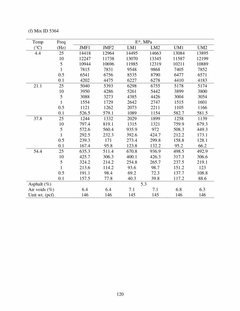
120

(f) Mix ID 5364

Temp Freq E*, MPa


4.4 25 14418 12964 14495 14663 13084 13895

10 12247 11738 13070 13345 11587 12199

5 10944 10696 11985 12319 10211 10889

1 7815 7831 9548 9868 7405 7852

0.5 6541 6756 8535 8790 6477 6571

0.1 4202 4475 6227 6278 4410 4183

21.1 25 5040 5393 6298 6755 5178 5174

10 3950 4286 5261 5442 3899 3800

5 3088 3273 4385 4426 3004 3054

1 1554 1729 2642 2747 1515 1601

0.5 1121 1262 2073 2211 1105 1166

0.1 526.5 579.1 1089 1154 582.7 581.5

37.8 25 1244 1332 2029 1899 1258 1139

10 797.4 819.1 1315 1321 759.9 679.3

5 572.6 560.4 935.9 972 508.3 449.3

1 292.5 232.3 392.6 424.7 212.2 173.1

0.5 239.3 171 273.4 299.8 158.8 128.1

0.1 167.4 95.8 123.8 132.2 95.2 66.2

54.4 25 635.3 511.4 670.8 936.9 498.5 492.9

10 425.7 306.3 400.1 426.3 317.3 306.6

5 324.2 214.2 254.8 265.7 237.5 219.1

1 213.6 114.2 93.6 98.7 151.2 123

0.5 191.1 98.4 69.2 72.3 137.7 108.8

0.1 157.5 77.8 40.3 39.8 117.2 88.6

Asphalt (%) 5.3

Air voids (%) 6.4 6.4 7.1 7.1 6.8 6.3

Unit wt. (pcf) 146 146 145 145 146 146

121

(g) Mix ID 5408

Temp Freq E*, MPa


4.4 25 14747 13904 12472 13676 14998 13988

10 13186 12285 11050 11917 13193 12800

5 12006 10915 9724 10613 11982 11522

1 9140 8073 7039 7783 8876 8188

0.5 7891 7022 6100 6520 7581 6944

0.1 5317 4649 4088 4268 4806 4519

21.1 25 6378 5699 5189 5244 5967 5728

10 4918 4436 4040 4159 4491 4304

5 4025 3497 3242 3333 3497 3426

1 2348 1904 1702 1763 1923 1756

0.5 1793 1386 1252 1287 1449 1245

0.1 907.8 659.5 564.1 596.2 663.1 541.1

37.8 25 2217 1490 1359 1544 1502 1459

10 1425 929.8 834 982.3 950.5 885.6

5 1022 636.4 563.8 678.9 664.5 593.5

1 452 247.3 226.4 291.4 304.8 238

0.5 324.1 172.8 158.3 212.9 234.5 172.4

0.1 157.8 83.8 71.2 113.6 140.6 92.9

54.4 25 741.8 785.4 490.1 513.5 500.8 516.3

10 376.4 434.8 271.3 281 280 327.5

5 236.7 275.6 172.7 178.9 184.7 236.2

1 95.9 100.2 60.8 64.6 68.6 133.4

0.5 73.7 76.5 46.5 79.4 54.2 115.4

0.1 45.1 47.6 28.6 51 35 88.7

Asphalt (%) 5.3

Air voids (%) 7.4 7.3 7.9 7.8 7.2 7.5

Unit wt. (pcf) 146 146 145 145 146 146

122

Table A1.2 Viscosity of asphalt binders at standard test temperatures

Viscosity (cP)

5381 5295 5192 5373 5627 5364 5408

Temp

° C

58-22 70-22 64-22 70-28 64-28 58-22 64-28

4.4 9.51x107

1.45x108

3.78x108 1.43x10

7 2.94x10

7 6.04x10

7 6.01x10

7

12.7 5.51x106

1.10x107

1.60x107

1.66x106

2.40x106

4.03x106

3.98x106

21.1 5.05x105

1.20x106

1.14x106

2.57x105

2.87x105

4.11x105

4.03x105

29.4 7.27x104

1.94x105

1.36x105

5.45x104

5.03x104

6.40x104

6.26x104

37.8 1.42x104

4.03x104

2.29x104

1.42x104

1.14x104

1.33x104

1.30x104

46.1 3.70x103

1.08x104

5.31x103 4.58x10

3 3.32x10

3 3.61x10

3 3.52x10

3

54.4 1.19x103

3.45x103

1.56x103

1.71x103

1.16x103

1.20x103

1.17x103

123

Table A1.3: Master curve fitting parameters

Mix Fitting

parameter


5381 χ 0.429752 0.723597 0.685327 1.094173 1.412442 1.107084

α 3.760578 3.505684 3.522654 3.18061 2.771668 3.190491

β -1.53895 -1.29788 -1.23332 -0.96776 -0.75969 -0.84595

γ 0.604881 0.706093 0.665885 0.715226 0.829887 0.62152

c 1.237558 1.0693 1.088817 0.858737 1.04894 1.053801

5295 χ 0.754426 0.739572 2.097732 1.115056 1.349815 0.850646

α 3.540724 3.525531 2.121062 3.174893 2.97311 3.516116

β -1.21295 -1.4508 -0.57006 -0.94547 -1.04119 -1.26753

γ 0.589617 0.584911 0.717185 0.713823 0.580509 0.571712

c 1.118277 1.210963 1.089971 0.895927 1.173026 1.112086

5192 χ 0.717671 1.577324 1.32258 0.838219 0.611667 0.82866

α 3.532344 2.795282 2.882083 3.415631 3.61956 3.512376

β -1.54077 -0.68855 -1.01487 -1.4876 -1.37461 -1.30994

γ 0.605617 0.759926 0.698459 0.677857 0.653291 0.611534

c 1.070714 0.65738 0.939002 0.862534 1.040376 0.921389

5373 χ 0.951054 1.06223 0.984625 1.462069 0.94939 1.356004

α 3.352918 3.211286 3.395035 2.799761 3.128716 2.925591

β -0.9497 -0.73676 -0.52767 -0.58053 -0.82761 -0.34539

γ 0.492612 0.587209 0.560918 0.59849 0.597303 0.627483

c 1.446028 1.113646 1.086728 1.289935 1.576219 1.151558

5627 χ 0.720986 0.61706 0.870989 0.740363 1.010413 0.685796

α 3.527131 3.665471 3.433698 3.5238 3.251023 3.653522

β -1.43743 -1.26066 -1.19168 -1.21507 -1.15226 -1.12177

γ 0.604239 0.638959 0.578819 0.636242 0.659386 0.635165

c 1.194188 1.101545 1.05 1.015378 1.121583 1.016377

5364 χ 2.062348 1.629383 0.657738 0.599883 1.875792 1.692657

α 2.171295 2.533179 3.573183 3.642303 2.264939 2.491587

β 0.010771 -0.48116 -1.20807 -1.24136 -0.24289 -0.31901

γ 0.871458 0.831703 0.607851 0.60718 0.91855 0.865757

c 0.936438 0.982732 1.095646 1.072552 0.969752 0.969007

5408 χ 0.654177 1.076748 0.724261 1.170639 0.544068 1.719066

α 3.604997 3.182946 3.460911 3.039655 3.798391 2.475911

β -1.12988 -0.74576 -0.92331 -0.74213 -0.93878 -0.38433

γ 0.585194 0.699142 0.663697 0.679031 0.53111 0.878477

c 1.051831 0.907786 0.987328 1.012931 1.096855 0.939319

124

Table A1.4: Viscosity regression coefficients

Mix Binder grade A VTS

5381 PG 58-22 16.4394 -5.7574

5295 PG 70-22 14.5301 -5.0462

5192 PG 64-22 17.039 -5.9679

5373 PG 70-28 13.7993 -4.7966

5627 PG 64-28 15.3901 -5.3792

5364 PG 58-22 16.0001 -5.5986

5408 PG 64-28 16.0605 -5.6210

125

APPENDIX 2

SAMPLE DYNAMIC MODULUS CURVES

4.4 °C

21.1 °C

37.8 °C

54.4 °C

1

10

100

1000

10000

100000

0.1 1 10 100

Frequency, Hz

E*,

MP

a

21.1 °C - reference

Figure A2.1: Typical raw dynamic modulus data measured at different temperatures and

frequencies

1

10

100

1000

10000

100000

0.00001 0.001 0.1 10 1000 100000

Frequency, Hz

E*,

MP

a

Figure A2.2: Master curve constructed by shifting the curves in Fig. A1.1 with reference to

21.1°C

126

1

10

100

1000

10000

100000

0.00001 0.001 0.1 10 1000 100000

Frequency, Hz

E*,

MP

a

measured

fitted

Figure A2.3: Master curve after sigmoidal curve fitting

127

APPENDIX 3

ANALYSIS OF VARIANCE – BASIC TERMINOLOGIES

A3.1 Treatment Factor

Treatment factor is any substance or item whose effect on the data is studied. The levels

are the specific types or amounts of the treatment factor in the experiment. For example, a

treatment factor might be a drug in a study whose levels are the different amounts of the drug

studied. In an experiment, there can be one or many treatment factors each having its own levels.

If two or more treatment factors are involved in an experiment then the combination of treatment

factors is a ‘treatment combination’ or simply ‘treatment’. For example, in a dynamic modulus

test, temperature and frequency are the two treatment factors. Each temperature and frequency

combination, say 4.4 °C and 25 Hz, is a treatment combination or treatment.

A3.2 Response

Response or response variable is the outcome of the study. Obviously, it is dependent

upon the levels of the treatment factors. For instance, dynamic modulus is a response dependent

on temperature and frequency.

A3.3 Experimental Units

Experimental units are the “material” to which the levels of the treatment factor(s) are

applied. For example, HMA test specimens are the experimental units in a study investigating

dynamic modulus of different mixes.

128

A3.4 Model

A model is a mathematical representation of the dependence of the response variable

upon the levels of the treatment factors. The model expresses the response variable (Y) as a

linear sum of the true response, denoted by µ, and the error variable or residual error, denoted

by ε. Linear models provide reasonably good approximations and are used extensively. Eq.A3.1

shows the mathematical form of a typical linear model.

εµY += ....................................................................... (A3.1)

Any model that takes the form similar to Eq.A3.1 is a linear model. This model is valid

for a case involving a single treatment factor. If two or more treatment factors are involved, the

model takes the form shown in Eq.A3.2.

itiit εµY += ................................................................. (A3.2)

where,

t = 1,…, ri, i = 1,…, v.

v is the number of treatments, t is the experimental unit in question, and ri is the number of

observations taken on the ith treatment.

For example, if dynamic modulus (E*) is the response, temperature and frequency are the

treatment factors, and two replicates were tested, the model can be written as,

E*it = µ + εit

i = 1, 2 (1 – temperature; 2 – frequency); t = 1, 2 (two replicates); ri = 2 (two replicates)

129

A3.5 Testing Equality of Treatment Effects

In an experiment involving many treatments, a common objective is to test whether or

not the treatments differ in terms of their effects on the response variable. Two hypotheses are

possible – null hypothesis and alternative hypothesis. Null hypothesis (H0) exists if the treatment

effects are all equal; alternative hypothesis (HA) exists if the treatment effects differ (at least two

of the treatment effects differ). For example, if dynamic modulus of different mixes is compared,

null hypothesis will exist if dynamic modulus of the mixes does not vary (i.e., Emix1 = Emix2 = …

= Emix7). If dynamic modulus of all or at the least two of the mixes differs then alternative

hypothesis exists (i.e., Emix1 ≠ Emix2 ≠ … ≠ Emix3). H0 is either accepted or rejected depending

upon p-value. If the computed p-value is less than the significance level (α) (see section A3.6),

H0 is rejected.

i.e., reject H0 if p < α.

A3.6 Significance Level (α)

It is the probability of rejecting H0 (i.e., the treatment effects are equal) when it is

actually true (HA) – this is called a Type I error. Generally, α is set before testing the hypothesis.

It should be small if it is important not to commit a Type I error (typical choices are α = 0.01 and

0.001); otherwise, a larger value can be chosen (typical choices are α = 0.01 and 0.05).

A3.7 P-value

In simple terms, p-value is the smallest level of significance that would lead to rejection

of the null hypothesis H0; most computer programs for statistical analysis report p-values. For

example, if the specified level of significance (α) is 0.01 and if p-value from the software is

130

0.0001, H0 exists. In this study, the statistical software SAS Version 9.1 is used for computing p-

values. Any textbook on analysis and design of experiments will explain the procedure for

computing p-value.

A3.8 Analysis of Variance (ANOVA)

Section A3.4 showed that any observed response can be expressed as the linear sum of

true response µ and residual error ε. If in an experiment, there are n responses each response will

differ/deviate from the true response µ by some error εt (where t refers to the response under

question). Obviously, the question of interest would be “How big are the errors?” Analysis of

Variance or ANOVA is the method used for measuring the error size important in p-value

computations. If the experiment involves a single treatment factor, it is a case of single-factor

ANOVA. If more than one treatment factor is involved, it is a case of multi-factor ANOVA.

ANOVA can be performed using statistical software like SAS, which is used in this study.

A3.9 Repeated Measures ANOVA

It is a special case when the experiment involves testing of all treatment factors or all

levels of the treatment factor(s) on a single experimental unit; the treatment factors are called

repeated measures. For example, in a dynamic modulus test a single specimen is tested under all

temperatures and frequencies. This requires a different statistical approach, which is the repeated

measure ANOVA. On the other hand, if the test uses a different specimen for different

temperatures and frequencies, say one specimen for 4.4°C and 25 Hz, and a different specimen

for 4.4°C and 10Hz, it becomes a case of standard ANOVA explained in Section A2.6.

131

A3.10 Tukey’s Multiple Comparison Method

This method is best for all pairwise comparisons. Pairwise comparison means comparing

each item with the rest of the items in the population. For example, in this study one of the

objectives was to test if the seven JMF mixes produced significantly different dynamic modulus.

Pairwise comparison here means comparing the dynamic modulus of each JMF mix with the

dynamic modulus of the other mixes i.e. JMF1 vs. JMF2, JMF1 vs. JMF3 etc.

Tukey’s method computes p-values by first computing confidence intervals for all

pairwise comparisons. Confidence interval is the upper and lower limit within which the

response of one treatment will differ from the other treatment. For example, consider a study

conducted to determine the effect of number of revolutions per minute (rpm) of a pump on the

fluid flow rate (in liters per minute). If after comparing 75 rpm and 50 rpm the confidence

interval was found to be (0.53, 0.64). Here, 0.64 is the upper limit and 0.53 is the lower limit

indicating that the fluid flow rate at 75 rpm will vary between 0.53 and 0.64 liters per minute

greater than at 50 rpm. This is confidence interval for a single contrast. If many contrasts are

involved, confidence intervals for all the pairwise comparisons can be determined using Tukey’s

multiple comparison method. Tukey’s method uses the confidence intervals of all pairwise

comparisons to determine p-values for each pairwise comparison.

132

APPENDIX 4

DISTRESS DATA COLLECTION1

A4.1 Data Collection

Pavement condition data is collected using a specialized pavement condition van (PCV),

illustrated in Fig. A4.1. A two-person team, driving at the posted speed limit, operates the PCV.

The PCV is equipped with six cameras that capture digital images of the driver’s perspective, the

right shoulder view, and the full width of the pavement surface. The driver’s perspective and

right shoulder view cameras are placed above the windshield of the PCV; two pairs of cameras

capture the roadway surface, placed on extension arms at the front and at the rear of the PCV.

The arrangement of the cameras is illustrated in Figure A4.2. The pavement image is captured

using one pair of cameras, each photographing half of the 12-foot lane. Each camera captures an

image 5x6.5 ft wide; images are captured every 25 feet. Depending on the angle of the sun, either

the front cameras or the rear cameras are selected to minimize shadows on the pavement surface

images. This arrangement of cameras and the captured images are used for characterizing surface

distresses (cracking, patching, etc.).

In addition to surface distress, it is also important to quantify the surface characteristics

that affect the roadway user. These characteristics are a measure of roadway roughness (roadway

profile in the longitudinal direction), rutting/wear (variation of roadway surface in the transverse

direction), and faulting. The roadway profile and rutting/wear measurements are collected via

laser sensors mounted on the front and rear of the pavement condition van. The PCV is equipped

with a profile bar, illustrated in Figure A4.2-(a), comprising laser sensors and accelerometers for

1 Pierce, L.M. (2008). Washington State Department of Transportation, State Pavement Engineer, Personal

Communication, May 2008.

133

measuring the longitudinal profile, from which roughness and faulting are calculated. The INO

laser illustrated in Figure A4.2-(b) measures rutting/wear transversely across the pavement

surface. The INO laser system consists of two laser line profilers (each capturing one-half of the

roadway width) and a special camera for measuring deformations (rutting or wear) of the laser

line profile.

A4.2 Data Analysis

The pavement profile and INO data is processed via computer programs, for

determination of roughness, faulting and maximum wheel path wear depth. Processing of the

digital images is a much more time consuming operation, since it requires review of each

pavement image by trained pavement rating staff. Review of pavement condition images are

accomplished via a specially developed computer program (PathView II) that allows the

pavement rating staff to view images for the driver’s perspective, the right shoulder view and the

pavement view on one screen, illustrated in Figure A4.3. In Figure A4.3, the upper left hand

image is the driver’s perspective view, the upper right hand image is the right shoulder view, and

the lower images are of the full lane width of the pavement surface.

The digital images are viewed one by one for a variety of pavement distress (cracking,

patching, spalling, etc.) types. The pavement rating staff, using a specially coded keyboard,

views the digital image for any pavement distress and use keystrokes that correspond to the

noted distress. The computer program records the keystroke and beginning and ending milepost

locations of each distress. Once the pavement distress rating is complete, the data is processed

for determination of type and length of distress and summed of 0.10 mile increments.

134

Figure A4.1 WSDOT pavement condition van.

(a) Front of van (b) Rear of van

Figure A4.2 Arrangement of cameras and sensors.

135

Figure A4.3 Sample image of pavement condition survey.

dynamic modulus test – laboratory … · 2008-07-15 · the objectives of this study were to...

Documents