dynamic network modeling and analysis of large- …
TRANSCRIPT
The Pennsylvania State University
The Graduate School
College of Engineering
DYNAMIC NETWORK MODELING AND ANALYSIS OF LARGE-
SCALE INTERNET OF THINGS WITH MANUFACTURING AND
HEALTHCARE APPLICATIONS
A Dissertation in
Industrial and Manufacturing Engineering
by
Chen Kan
© 2018 Chen Kan
Submitted in Partial Fulfillment
of the Requirements
for the Degree of
Doctor of Philosophy
May 2018

ii
The dissertation of Chen Kan was reviewed and approved* by the following:
Hui Yang
Harold and Inge Marcus Career Associate Professor of Industrial and Manufacturing Engineering
Dissertation Co-Advisor, Co-chair of Committee
Sounder Kumara
Allen E. Pearce and Allen M. Pearce Professor of Industrial and Manufacturing Engineering
Dissertation Co-Advisor, Co-chair of Committee
Jingjing Li
William and Wendy Korb Early Career Professor (Associate Professor) of Industrial and
Manufacturing Engineering
Lin Lin
Assistant Professor of Statistics
Janis Terpenny
Peter and Angela Dal Pezzo Department Head and Professor of Industrial and Manufacturing
Engineering
*Signatures are on file in the Graduate School

iii
Abstract
With the advancement of sensing and information technology, sensor networks and imaging
devices have been increasingly used in manufacturing and healthcare to improve information
visibility and enhance operational quality and integrity. Furthermore, the Internet of Things (IoT)
technology has been integrated for the continuous monitoring of machine and patient conditions.
As such, large amounts of data are generated with high dimensionality and complex structures.
This provides an unprecedented opportunity to realize smart automated systems such as smart
manufacturing and connected health care. However, it also raises new challenges in data analysis
and decision making. Realizing the full potential of the data-rich environment calls for the
development of new methodologies for data-driven information processing, modeling, and
optimization.
This dissertation develops new methods and tools that enable 1) better handling of large
amounts of multi-channel signals and imaging data generated from advanced sensing systems in
manufacturing and healthcare settings, 2) effective extraction of information pertinent to system
dynamics from the complex data, and 3) efficient use of acquired knowledge for performance
optimization and system improvement. The accomplishments include:
1) Fusion and analysis of multi-channel signals. In Chapter 2, a spatiotemporal warping
approach was developed to characterize the dissimilarity among 3-lead functional
recordings. A network was then optimally constructed based on the dissimilarity and
network features were extracted for the identification of different types of diseases.
2) Statistical process control based on time-varying images. In Chapter 3, a stream of time-
varying images were represented as a dynamic network. Then, community structure of the
network was characterized and community statistics were extracted from time to time.
Finally, a new control charting approach was developed for in-situ monitoring of
manufacturing processes.
3) Monitoring and Control of large-scale Industrial Internet of Things. In Chapter 4, a
stochastic learning approach was developed to construct a large-scale dynamic network
from IIoT machines. A parallel computing scheme was further proposed to harness

iv
multiple computation resources to increase the efficiency. The constructed large-scale
network can be used to visually and analytically monitor machine condition, inspect
product quality, and optimize manufacturing processes.
4) Modeling and Analysis of large-scale Internet of Health Things. In Chapter 5, the large-
scale network model was extended to the Internet of Health Things. A new IoT technology
specific to the heart disease, namely, the Internet of Hearts, was proposed. Dynamic
network modeling and parallel computing schemes were designed and developed for multi-
level cardiac monitoring: patient-to-patient variations in the population level and beat-to-
beat dynamics in the individual patient level. Control charting schemes were further
proposed to harness network features for change detection in the cardiac processes.

v
Contents List of Figures ............................................................................................................................. viii
List of Tables ............................................................................................................................... xii
Acknowledgements .................................................................................................................... xiii
Chapter 1 : Introduction .............................................................................................................. 1
1.1. Motivation ..................................................................................................................................... 1
1.2. State-of-the-Art ............................................................................................................................. 2
1.3. Research Objectives ...................................................................................................................... 4
1.4. Organization of the Dissertation ................................................................................................... 4
Chapter 2 : Dynamic Spatiotemporal Warping for the Detection and Location of
Myocardial Infarctions ................................................................................................................. 7
2.1. Introduction ................................................................................................................................... 7
2.2. Research Methodology ............................................................................................................... 10
A. Dynamic Spatiotemporal Warping .............................................................................................. 10
B. Spatial Embedding ...................................................................................................................... 15
C. Self-organizing Map .................................................................................................................... 17
2.3. Materials and Experimental Results ........................................................................................... 18
A. Influence of embedding dimension .............................................................................................. 19
B. Influence of neuron map size ...................................................................................................... 20
C. Hierarchical Classification ......................................................................................................... 21
2.4. Conclusion and Discussions........................................................................................................ 22
Chapter 3 : Dynamic Network Modeling and Control of in-situ Image Profiles from
Ultraprecision Machining and Biomanufacturing Processes ................................................. 24
Abstract ................................................................................................................................................... 24
3.1. Introduction ................................................................................................................................. 25
3.2. Research Background ................................................................................................................. 26
A. Profile Monitoring ...................................................................................................................... 26
B. Image Profiles ............................................................................................................................. 28
3.3. Research Methodology ............................................................................................................... 29
A. Network Representation of Image Profiles ................................................................................. 29
B. Network Community Modeling and Characterization ................................................................ 30
C. Multivariate Monitoring of Network Statistics ........................................................................... 33
3.4. Experiments and Results ............................................................................................................. 37
A. Case Study in the Biomanufacturing Process ............................................................................. 37
B. Case Study in Ultra-Precision Machining .................................................................................. 47

vi
3.5. Discussion and Conclusions........................................................................................................ 52
Chapter 4 : Parallel Computing and Network Analytics for Fast Industrial Internet-of-
Things (IIoT) Machine Information Processing and Condition Monitoring ........................ 54
Abstract ................................................................................................................................................... 54
4.1. Introduction ................................................................................................................................. 55
4.2. Research Background ................................................................................................................. 59
A. Advanced Sensing and Condition Monitoring ............................................................................ 59
B. Industrial Internet of Things ....................................................................................................... 61
C. Serial Computing vs. Parallel Computing .................................................................................. 62
4.3. Research Methodology ............................................................................................................... 64
A. Pattern Matching and Signature Warping .................................................................................. 65
B. Network Embedding and Predictive Modeling of Machine Signatures ...................................... 67
C. New Algorithms for Large-scale Network Modeling .................................................................. 68
4.4. Experiments and Results ............................................................................................................. 73
A. Optimization of a Large-scale Machine-to-Machine Network ....................................................... 74
B. Optimization of a Cycle-to-Cycle Network Customized to One Machine ...................................... 76
4.5. Conclusion and Discussions........................................................................................................ 79
Chapter 5 : Parallel Computing for Multi-level Modeling and Analysis of the Large-scale
Internet of Health Things ........................................................................................................... 82
Abstract ................................................................................................................................................... 82
5.1. Introduction ................................................................................................................................. 83
5.2. Research Background ................................................................................................................. 85
A. Cardiac Monitoring and Pattern Recognition ............................................................................ 85
B. The Internet of Health Things ..................................................................................................... 86
5.3. The Internet of Hearts ................................................................................................................. 88
A. IoH Architecture ......................................................................................................................... 88
B. IoT Sensing and the Physical Network of Patients ..................................................................... 88
C. The Virtual Network of Patients .................................................................................................. 90
D. Multi-level Networks Modeling and Analysis of Beat-to-beat (B2B) Dynamics and Patient-to-
patient (P2P) variations. ..................................................................................................................... 91
5.4. Network Analytics of the Internet of Hearts ............................................................................... 93
A. Dissimilarity Measure ................................................................................................................. 94
B. Data-driven Modeling and Optimization of a Large-scale Dynamic Network ........................... 95
C. Network-based Monitoring of Cardiac Processes .................................................................... 100
5.5. Materials and Experimental Design .......................................................................................... 101

vii
5.6. Experimental Results ................................................................................................................ 103
A. Simulation Studies ..................................................................................................................... 103
B. Real-world Studies .................................................................................................................... 107
5.7. Discussion and Conclusions...................................................................................................... 109
Chapter 6 : Conclusions and Future Research ...................................................................... 112
Appendix .................................................................................................................................... 116
Appendix A – Proof of Proposition 1 in Chapter 3 ............................................................................... 116
Appendix B – Proof of Proposition 2 in Chapter 3 ............................................................................... 118
Appendix C – Copyright Permissions ................................................................................................... 120
References .................................................................................................................................. 126

viii
List of Figures
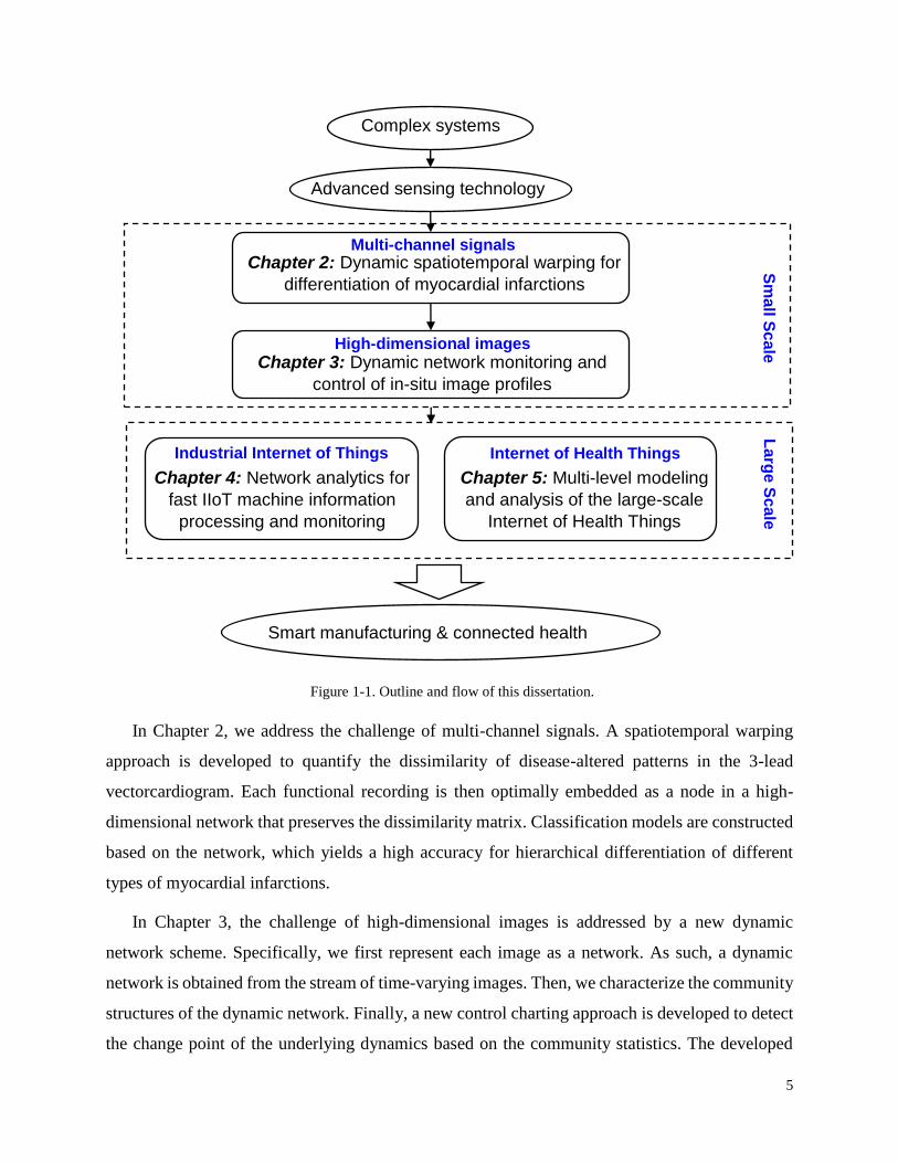
Figure 1-1. Outline and flow of this dissertation. ........................................................................... 5
Figure 2-1. Cardiac electrical activities of HC (blue/solid) and MI subjects (red/dashed). ........... 8
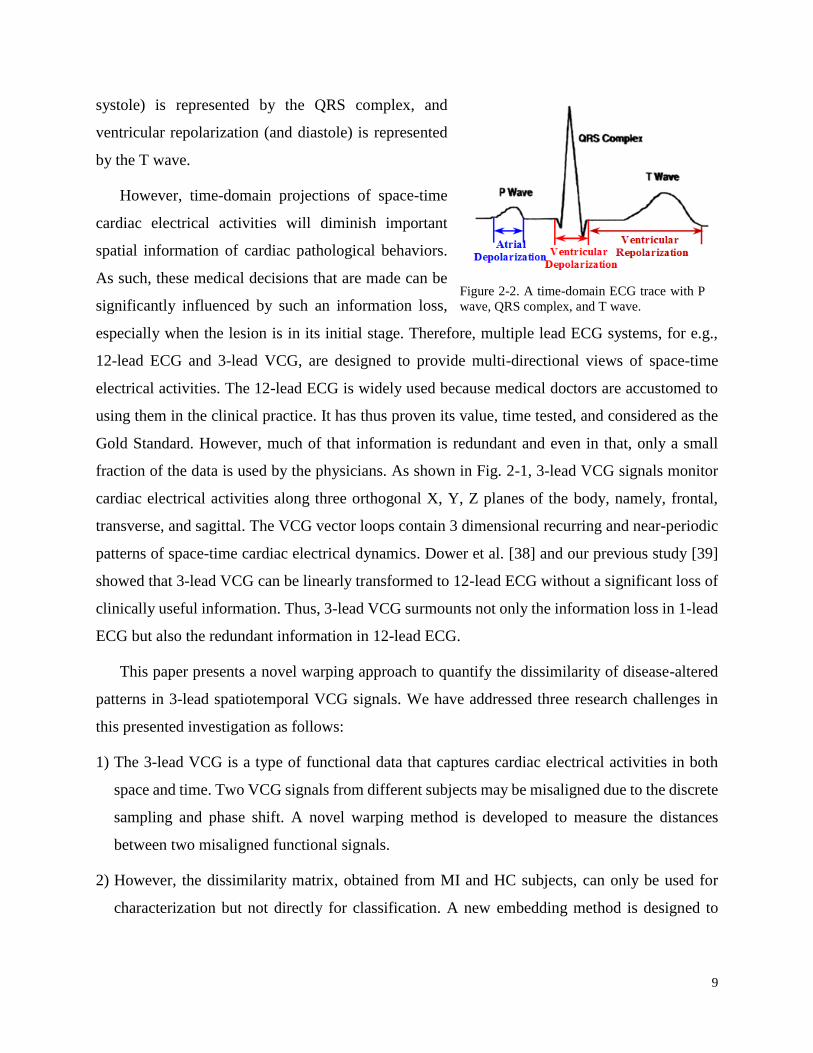
Figure 2-2. A time-domain ECG trace with P wave, QRS complex, and T wave. ......................... 9
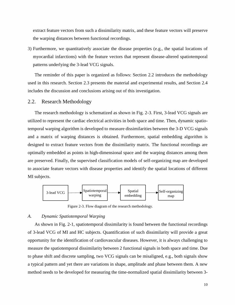
Figure 2-3. Flow diagram of the research methodology. .............................................................. 10
Figure 2-4. (a) Labels between each pair of groups in the warping distance matrix; (b) Color
mapping plot of the warping distance matrix. ......................................................... 12
Figure 2-5. Spatial embedding algorithm; (a) original distance matrix ∆; (b) network and nodes;
(c) Reconstructed distance matrix D. ....................................................................... 16
Figure 2-6. (a) 2-D and (b) 3-D visualization of spatial embedding vectors for HC and MI subjects.
.................................................................................................................................. 17
Figure 2-7. Structure of hierarchical classification ....................................................................... 19
Figure 2-8. Stress values for the embedding dimensions from 1 to 16......................................... 20
Figure 2-9. Response surface of AICc for different SOM map sizes. .......................................... 21
Figure 2-10. (a) SOM U-matrix for the neuron distances; (b) SOM sample hits plot; (c) SOM
Neuron labels of HC (blue) and MI (red) ................................................................ 22
Figure 3-1. (a) Ultra-Precision Machining; (b) whole-heart optical mapping. ............................. 25
Figure 3-2. Flow chart of the research methodology. ................................................................... 29
Figure 3-3. Examples of community detection using the Hamiltonian algorithm. (a) original
images; (b) two communities; (c) ten communities. ................................................ 33
Figure 3-4. Multivariate network GLR statistics in the eigenspace.............................................. 36
Figure 3-5. (a) Real-world image of a cell in the biomanufacturing process; (b) Out-of-control
image with a vesicle (size r = 6); (c) Out-of-control image with a vesicle (size r = 4).
.................................................................................................................................. 38
Figure 3-6. (a) Community detection result of a cellular image (15 communities), (b) Normal
probability plot of pixel intensities in the 15th community. ..................................... 39
Figure 3-7. Normal probability plots of image-to-image (a) mean intensities (b) standard deviation
of intensities (c) number of pixels in the 15th community for a stream of dynamic
images. ..................................................................................................................... 39
ix
Figure 3-8. (a) Square-shaped ROI in the cellular image, (b) Normal probability plot of pixel
intensities within the square ROI. ............................................................................ 40
Figure 3-9. (a) Pixel intensity variations in the square ROI with respect to time, and normal
probability plots of image-to-image (b) mean intensities (c) standard deviation of
intensities (d) number of pixels within the square ROI for a stream of dynamic image
profiles. .................................................................................................................... 41
Figure 3-10. The performance of GLR control chart with square-shaped ROIs for the monitoring
of biomanufacturing process. ................................................................................... 41
Figure 3-11 Pareto chart of the percentage of variance explained by principal components of the
Q-variate vector of network community statistics. .................................................. 46
Figure 3-12. (a) Linear roughness measurement (roughness trace is marked in red); (b) Two
distinct roughness traces (black/solid) with same Ra values. ................................... 48
Figure 3-13. Surface images from UPM process, (a) a smooth surface with surface roughness Ra
= 43nm; (b) a rough surface with Ra = 585 nm; (c) community detection results of
the smooth surface in (a); (d) community detection results of the rough surface in (b).
.................................................................................................................................. 49
Figure 3-14. Distribution of community statistics – the percentage of pixels vs. average pixel
amplitude in each community for (a) Smooth surface with Ra = 43nm; (b) Rough
surface with Ra = 585nm. ......................................................................................... 50
Figure 3-15. Scatter plot of Ra values and GLR statistics from 80 images. ................................. 51
Figure 3-16. Distributions of community statistics – the percentage of pixels vs. average pixel
amplitude in each community for two rough surfaces. ............................................ 52
Figure 4-1. (a) The power profile of a turning machine; (b) The machined part (JIS S45C). ..... 56
Figure 4-2. Cycle-to-cycle variations of power profiles in a single machine. .............................. 57
Figure 4-3. A machine-to-machine network in the IIoT. ............................................................. 58
Figure 4-4. Machine-network information processing: (a) Serial computing on a single processor
vs. (b) Parallel computing on multiple processors. .................................................. 63
Figure 4-5. The proposed methodology for condition monitoring of IIoT machines. ................. 64
Figure 4-6. Power consumptions of two turning processes. ........................................................ 65
Figure 4-7. (a) Direct pattern matching of misaligned signatures; (b) Optimal pattern matching of
aligned signatures by the dynamic time warping. .................................................... 66

x
Figure 4-8. (a) Dissimilarity matrix of six machine signatures; (b) An embedded network with
node-to-node distances preserving the dissimilarity matrix in (a). .......................... 67
Figure 4-9. The computation time of stochastic network embedding and classic multidimensional
scaling in a single computing unit. .......................................................................... 74
Figure 4-10. The convergence of stochastic network embedding. .............................................. 75
Figure 4-11. Performance comparison of parallel (12 cores) and serial computing. .................... 76
Figure 4-12. A Haas ST-20Y turning center at the Pennsylvania State University. .................... 77
Figure 4-13. A worn (left) and a new (right) coated tungsten carbide cutting tools..................... 77
Figure 4-14. Morphology of power profiles in the cutting phase for three conditions in the turning
process...................................................................................................................... 78
Figure 4-15. Visualization of a 3-D network (nodes) embedded from 6000 turning cycles with 3
different conditions (Normal, Chatter and Tool wear). ........................................... 79
Figure 5-1. An Illustration of the Large-scale Internet of Hearts. ................................................ 88
Figure 5-2. Wireless communication protocols in the IoH. .......................................................... 89
Figure 5-3. Physical network to virtual network (P2V) communication in the IoH. .................... 90
Figure 5-4. (a) ECG dynamics within a patient (cycle-to-cycle) and (b) ECG variations among
multiple patients (patient-to-patient)........................................................................ 92
Figure 5-5. Cycle-to-cycle network (left) and patient-to-patient network (right) in the IoH. ...... 93
Figure 5-6. Flowchart of proposed big data analytics scheme in the virtual network of IoH. ..... 94
Figure 5-7. Experimental design of the simulation study. .......................................................... 103
Figure 5-8. Computation time using parallel and serial computing for (a) dynamic warping and (b)
stochastic network embedding. .............................................................................. 104
Figure 5-9. Performance comparison between three types of control charts under different shift
magnitudes for (a) shifted ST segments, (b) shifted P segments and (c) shifted QRS
segments. ................................................................................................................ 106
Figure 5-10. Performance comparison between three types of similarity measures (dynamic
warping, correlation and mutual information) under different shift magnitudes. .. 107
Figure 5-11. A segment of real-world ECG signals containing normal beats (N) and premature
ventricular contraction beats (V). .......................................................................... 107
Figure 5-12. The constructed beat-to-beat networks for (a) 15 beats; (b) 25 beats; and (c) 50 beats
from the real-world ECG signals. .......................................................................... 108

xi
Figure 5-13. The constructed beat-to-beat network with blue nodes representing normal beats and
read nodes representing premature ventricular contractions. ................................ 109

xii
List of Tables
Table 2-1. Two Sample t-Test for Testing the Mean of Spatiotemporal Distances at Different MI
Locations ..................................................................................................................... 13
Table 2-2. Two Sample F-Test for Testing the Variance of Spatiotemporal Distances at Different
MI Locations ............................................................................................................... 14
Table 2-3. Two Sample KS-Test for Testing the CDF of Spatiotemporal Distances at Different
MI Locations ............................................................................................................... 15
Table 2-4. The Variations of Correct Rates with Different SOM Map Sizes ............................... 20
Table 2-5. Hierarchical Classification Results .............................................................................. 21
Table 3-1. The Potts Model Hamiltonian Algorithm for Network Community Detection ........... 32
Table 3-2. Performance Comparison Between Network GLR and Hotelling T2 Charts .............. 44
Table 3-3. Performance Comparison of Multivariate Network GLR and T2 Charts in the Reduced
Dimension ................................................................................................................... 47

xiii
Acknowledgements
I would like to express my deepest gratitude to Dr. Hui Yang, my advisor, for his continuous
support, guidance, and care throughout my Ph.D. study. I will always remember his instructions
and help on how to design experiments, how to write papers, and how to give presentations. It is
Dr. Hui Yang who let me make up my mind to pursue an academic career. Also, I owe my sincere
gratitude to my co-advisor, Dr. Soundar Kumara, for this insightful guidance and encouragement.
Dr. Kumara’s rich knowledge, rigorous thinking, and professionalism have an immense impact on
my current and future research. Both Dr. Yang and Dr. Kumara are my role models. Through their
guidance and encouragement, I have grown both personally and professionally.
I would like to thank my other committee members, Dr. Jingjing Li and Dr. Lynn Lin for their
support on my research. No matter how busy they are, they always find time to meet and give me
valuable suggestions. They provide knowledge from different domains and their valuable
comments help me a lot to improve the quality of my dissertation. My deep gratitude also goes to
professors and scholars who helped me and/or worked collaboratively with me in the past few
years, including Dr. Fabio Leonelli, Dr. Changqing Cheng, Dr. Kay-Pong Yip, Dr. Prohalada Rao,
Dr. Tapas Das, Dr. Satish Bukkapatnam, Dr. Robert Voigt, and Dr. Janis Terpenny. Special thanks
to Dr. Jose Zayas-Castro for his encouragement and support during my Ph.D. study.
I greatly appreciate the opportunity to work in Dr. Hui Yang’s Complex Systems Monitoring,
Modeling and Analysis Laboratory. I would like to thank my fellow students and colleagues in the
lab, including but not limited to Dr. Dongping Du, Dr. Gang Liu, Dr. Yun Chen, Ms. Bing Yao,
Mr. Cheng-Bang Chen, Mr. Farhad Imani, Ms. Shengli Pei, and Ms. Rui Zhu. I would also like to
thank administrative staffs in the IME department Ms. Lisa Fuoss, Mr. James Wyland, Ms.
Laurette Gonet for their generous help. In addition, I gratefully acknowledge the financial support
from the National Science Foundation (CMMI-1454012, CMMI-1266331, CMMI-1619648, IIP-
1447289, and IOS-1146882) and other funding resources.
Most importantly, I wish to thank my beloved parents for their endless love and unconditional
support. Their encouragement and trust always help me get through difficulties in my life.
1
Chapter 1: Introduction
1.1. Motivation
The modern industries have increasingly invested in advanced sensing technology to cope with
the ever-increasing complexity of systems, improve the visibility of information, and enhance
operational quality and integrity. 1) Instead of single-channel sensing, distributed sensor networks
have been more and more used in manufacturing and healthcare to facilitate the all-round
collection of space-time information. For example, 12-lead electrocardiogram (ECG) system
deploys 10 electrodes to provide multi-directional views of cardiac electrical activity. Multiple
sensors (e.g., cutting force, vibration, and acoustic emission) are installed for in situ quality
assurance of ultra-precision machining (UPM). 2) Furthermore, imaging technologies are
increasingly adopted for online and high-resolution monitoring of process dynamics. High
dimensional functional images are collected to assess the quality of manufactured products or
study the pathology of diseases. For example, microscopic images have been used to inspect the
surface finish of UPM samples. Cardiac optical mapping captures emitted fluorescent lights from
the heart and produces time-varying 2-D and 3-D images for electrophysiological analysis. 3)
Recently, the Internet of Things (IoT) has been hailed as a revolution in automation science and
information technology. The IoT deploys a multitude of sensors, computing units and physical
objects in an Internet-like infrastructure. The cyber-physical system of IoT enables continuous
condition monitoring and timely anomaly detection in both manufacturing and healthcare settings.
As a result, advanced sensing brings rich data, which provides an unprecedented opportunity
to realize smart automated systems such as smart manufacturing and smart health care. However,
advanced sensing produces massive data with complex structures, which poses significant
challenges:
1) Distributed sensor networks capture spatiotemporal signals, which show high-level of
nonlinear and nonstationary patterns with the presence of extraneous noises. This hampers the
performance of traditional approaches with linearity and stationarity assumptions.
2) Imaging technology generates 2-D, 3-D, and higher-dimensional functional images. Most
of traditional statistical process control (SPC) approaches are designed for the monitoring of 1-D

2
profiles and they are limited in their ability to handle high-dimensional images for process
monitoring and fault diagnosis.
3) IoT connects large amounts of machines in digital manufacturing, as well as human subjects
in smart and connected health. This gives rise to large amounts of data with complex and
multifarious structures. Traditional approaches are limited in their ability to effectively extract
pertinent knowledge about system dynamics in the large-scale IoT contexts.
Therefore, realizing the full potential of the data-rich environment requires fundamentally new
methodologies for data-driven information processing, modeling, and optimization. There is a
pressing need to develop advanced methodologies and associated tools that will enable and assist
in 1) the handling of massive, complex data generated from advanced sensing systems in
manufacturing and healthcare settings; 2) the extraction of pertinent information about system
dynamics; and 3) the exploitation of acquired knowledge for decision making and performance
optimization.
1.2. State-of-the-Art
With sensor networks and imaging technology, high-dimensional data (such as multi-channel
signals and 2-D images) are increasingly available in manufacturing and healthcare. In the past
decade, various methods have been developed in the research community of Industrial Engineering
to extract useful information from the data for process monitoring and anomaly detection. The
typical idea is to reduce the high-dimensional data as representative features in the low-
dimensional space. To achieve this, one way is to represent the data by different models, and
further extract model parameters as features. See, for example, linear models of Kang and Albin
[1] , Kim et al. [2], and Zou et al. [3], and mixed-effect models of Apley [4] and Zhou et al. [5].
Also, some works apply dimensionality reduction techniques. For example, the principal
component analysis used by Paynabar et al. [6] and independent component analysis by Ding et
al. [7]. Furthermore, some papers transform the original data into other domains for feature
extraction. For example, wavelet decomposition by Yang [8] and Zhou et al. [9], and fractal
representation by Ruschin-Rimini et al. [10]. Methods such as variable selection (e.g., Liu and
Yang [11] and Sun et al. [12]) can then be applied to further reduce the size of the feature set. In
addition, other approaches (e.g., recurrence analysis of Chen and Yang [13], and Kan et al. [14])
are also developed in the literature to extract features from sensing signals. Although these works
3
made great contributions to the research in system informatics and quality engineering, they are
designed for the monitoring of 1-D signals and are limited in their ability to handle high-
dimensional images.
In the literature, pioneering works have been done to extract useful information from 2-D and
3-D profiles for process monitoring and control. Instead of directly using the imaging data, earlier
efforts are made to obtain representative sample points from 2-D profiles. For example, Jin et al.
[15] and Zhang et al. [16] collect a reduced set of thickness measurements to characterize the 2-D
geometric shape of a wafer. Some works studied the spectral bands of hyperspectral images. For
example, approaches were developed by Du et al. [17] and Wilcox et al. [18] to optimally select a
subset of spectral bands from hyperspectral images for quality control. Some papers directly handle
images or a sequence of images collected in the manufacturing process. For example, Yan et al.
[19] proposed a low-rank tensor decomposition to extract features from images for process
monitoring and anomaly detection. Megahed et al. [20] segmented the image into multiple regions
of interests and developed a generalized likelihood ratio chart to monitor the color shift in those
small regions. Yao et al. [21] proposed a 2-D multifractal analysis to characterize the surface
integrity of products based on CT scan images. However, most of these studies focus on fault
detection from snapshot images in discrete-part manufacturing. They are limited in their ability to
monitor the time-varying image profiles that are highly nonlinear and nonstationary.
Recently, there is an increasing interest in bringing IoT into manufacturing and healthcare to
increase the smartness level of the system. Some works have been done in the design of IoT-based
cloud manufacturing. For example, see the four-layer cloud manufacturing system developed by
Tao et al [22], real-time plant monitoring system by Georgakopoulos [23], and IoT-based
manufacturing resources perception and access by Tao et al. [24]. Some research focus on the
development of cyber-physical manufacturing systems. For example, the UML-based framework
(i.e., UML4IoT) proposed by Thramboulidis and Christoulakis [25] and feature-based
manufacturing system by Adamson et al. [26]. Some works leverage IoT technology for energy
efficiency management. For example, Qin et al. [27] implemented IoT in the optimization of energy
consumption in the additive manufacturing. Tan et al. [28] used IoT for the real-time monitoring of
energy efficiency on manufacturing shop floors. Furthermore, IoT technology has been applied in
manufacturing operations management. Xu and Chen [29] developed an IoT-based dynamic
production scheduling framework for just-in-time manufacturing. Ding et al. [30] developed an

4
approach for optimal allocation of sensors in a multi-station assembly process. In addition, some
research have been conducted to achieve IoT-enabled connected healthcare. For example, Pasluosta
et al. [31] presented an IoT-enabled solution for the diagnosis and treatment of Parkinson’s disease.
Al-Taee et al. [32] developed a mobile health platform to incorporate humanoid robots for the
management of diabetes in children. Islam et al. [33] presented a comprehensive survey on IoT-
enabled healthcare applications. However, most of these works focus on the conceptual design of
IoT infrastructures or hardware development. Little has been done to leverage sensing data from a
large-scale IoT to develop new methods and tools for process monitoring, diagnosis, and
improvement.
1.3. Research Objectives
The long-term goal of my research is to develop innovative sensor-based methodologies for
the modeling, monitoring, and optimization of large-scale complex systems. Specifically, the
objectives of this dissertation include:
1) Proposing a network model to optimally quantify the spatiotemporal dissimilarity among
multi-channel signals for the anomaly detection.
2) Developing a dynamic network methodology to represent, model and control of time-
varying image profiles for the in-situ process monitoring and quality control.
3) Developing a large-scale network model to efficiently handle big data in the Industrial
Internet of Things for machine information processing, condition monitoring, and fault
diagnosis.
4) Extending the large-scale network model for the multi-level modeling and analysis of the
Internet of Health Things.
1.4. Organization of the Dissertation
This dissertation is organized based multiple manuscripts. Each of chapters 2, 3, 4, and 5 is
written as a research paper, which has been published or under review. The outline of this
dissertation is illustrated in Fig. 1-1.
5
In Chapter 2, we address the challenge of multi-channel signals. A spatiotemporal warping
approach is developed to quantify the dissimilarity of disease-altered patterns in the 3-lead
vectorcardiogram. Each functional recording is then optimally embedded as a node in a high-
dimensional network that preserves the dissimilarity matrix. Classification models are constructed
based on the network, which yields a high accuracy for hierarchical differentiation of different
types of myocardial infarctions.
In Chapter 3, the challenge of high-dimensional images is addressed by a new dynamic
network scheme. Specifically, we first represent each image as a network. As such, a dynamic
network is obtained from the stream of time-varying images. Then, we characterize the community
structures of the dynamic network. Finally, a new control charting approach is developed to detect
the change point of the underlying dynamics based on the community statistics. The developed
Advanced sensing technology
High-dimensional images
Chapter 3: Dynamic network monitoring and
control of in-situ image profiles
Industrial Internet of Things
Chapter 4: Network analytics for
fast IIoT machine information
processing and monitoring
Chapter 5: Multi-level modeling
and analysis of the large-scale
Internet of Health Things
Internet of Health Things
Complex systems
Chapter 2: Dynamic spatiotemporal warping for
differentiation of myocardial infarctions
Multi-channel signals
Smart manufacturing & connected health
Sm
all S
cale
L
arg
e S
cale
Figure 1-1. Outline and flow of this dissertation.

6
dynamic network scheme shows its effectiveness on the monitoring of both UPM and
biomanufacturing processes.
In Chapter 4, we develop a large-scale network model to address the challenge of Industrial
Internet of Things (IIoT). We measure the dissimilarity among machine signatures and further
represent each machine signature as a node in the network. A stochastic learning approach is
developed to reduce the computational complexity of network embedding. Also, a parallel
computing scheme is developed to increase the computational efficiency for the embedding of
large amounts of IIoT-enabled machines. The developed approach shows a strong potential for
predictive maintenance and optimal machine scheduling in the context of IIoT.
In Chapter 5, we further extend the large-scale network model to address the challenge of the
Internet of Health Things. In this study, we propose a new IoT technology, namely the Internet of
Hearts (IoH), to empower the smart and connected heart health. We designed and developed a new
approach of dynamic network modeling and parallel computing for multi-level cardiac monitoring:
patient-to-patient variations in the population level and beat-to-beat dynamics in the individual
patient level. After the construction of the large-scale dynamic network, control charts are
proposed to harness network features for change detection of cardiac processes. The dynamic
network reveals important information pertinent to patients’ cardiac dynamics, which shows a
strong potential for real-time cardiac monitoring and disease management.
In the end, Chapter 6 concludes the dissertation and summarizes the contributions. Future
research directions are also discussed in this chapter.

7
Chapter 2: Dynamic Spatiotemporal Warping for the Detection and
Location of Myocardial Infarctions1
Abstract
Myocardial infarction (MI), also known as heart attack, is the leading cause of death – about
452,000 per year – in US. It often occurs due to the occlusion of coronary arteries, thereby leading
to the insufficient blood and oxygen supply that damage cardiac muscle cells. Because the blood
vessels are all over the heart, MI can happen at different spatial locations (e.g., anterior and inferior
portions) of the heart. The spatial location of diseases causes the variable excitation and
propagation of cardiac electrical activities in space and time. Most of previous studies focused on
the relationships between disease and time-domain biomarkers (e.g., QT interval, ST
elevation/depression, heart rate) from 12-lead ECG signals. Few, if any, previous approaches have
investigated how the spatial location of diseases will alter cardiac vectorcardiogram (VCG) signals
in both space and time. This paper presents a novel warping approach to quantify the dissimilarity
of disease-altered patterns in 3-lead spatiotemporal VCG signals. The hypothesis testing shows
there are significant spatiotemporal differences between healthy controls (HC), MI-anterior, MI-
anterior-septal, MI-anterior-lateral, MI-inferior, and MI-inferior-lateral. Further, we optimize the
embedding of each functional recording as a feature vector in the high-dimensional space that
preserves the dissimilarity distance matrix. This novel spatial embedding approach facilitates the
construction of classification models and yields an accuracy of 94.7% for separating MIs and HCs
and an accuracy of 96.5% for anterior-related MIs and inferior-related MIs.
2.1. Introduction
Myocardial infarction (MI), commonly known as a heart attack, is the leading cause of death
in US. It is reported that nearly 452,000 Americans die from MI each year and almost every 34
seconds, there will be a heart attack in the US. MI occurs due to the occlusion of the coronary
arteries. This results in the insufficient blood and oxygen supply that damages the cardiac muscle
1 This chapter has been published in IEEE International Conference on Automation Science and Engineering (CASE) 2012

8
cells and trigger the disease-induced degradation process. The
accurate detection of myocardial infarctions is critical for the
timely medical interventions and the improvement of quality of
life.
It is well known that cardiac electrical activities are spatio-
temporally excited and propagated, i.e., initially excited at the
sinoatrial (SA) node, conducted in both atria, then relayed
through the atrioventricular (AV) node to further propagate
through bundle of His and Purkinje fibers toward ventricular
depolarization and repolarization. Because MI takes place in
different spatial locations of the heart, e.g., anterior, inferior, space-time cardiac electrical
activities are often perturbed by the location of lesions in the heart. As shown in Fig. 2-1, the MI
and healthy control (HC) subjects show vastly dissimilar cardiac electrical activities in space and
time. The blue/solid trajectories represent the vectorcardiogram (VCG) signals from a HC subject,
and the red/dash trajectories are from a MI subject. Our previous studies demonstrated there are
statistically significant differences in spatiotemporal paths of cardiac electrical activities between
healthy and diseased subjects [8, 34, 35]. It may be noted that we developed the approaches of
multiscale recurrence analysis [35] and spatial octant analysis [36] for the characterization and
quantification of disease-altered cardiac electrical dynamics in space and time. However, few
progresses have been made previously to quantitatively measure spatiotemporal distances of VCG
signals between healthy and diseased subjects, and further utilize these distance measures to
identify the locations of myocardial infarctions.
Most of previous studies focused on the relationships between diseases and time-domain
biomarkers (e.g., QT interval, ST elevation or depression, heart rate) from ECG signals. As shown
in Fig. 2-2, the 1-lead ECG is obtained by measuring the potential difference between 2 electrodes
that are placed on the body surface (e.g., left foot, left arm and right arm). The ECG trace is often
temporally segmented into P wave, QRS complex, and T wave (see Fig. 2-2). Each segment is
closely associated with the specific physical activities of heart components [37]. For example,
atrial depolarization (and systole) is represented by the P wave, ventricular depolarization (and
Vz
HC337(3,4,5) vs Inferior-lateral44(7,8,9)
Vy
Vx
Figure 2-1. Cardiac electrical activities
of HC (blue/solid) and MI subjects
(red/dashed).
9
systole) is represented by the QRS complex, and
ventricular repolarization (and diastole) is represented
by the T wave.
However, time-domain projections of space-time
cardiac electrical activities will diminish important
spatial information of cardiac pathological behaviors.
As such, these medical decisions that are made can be
significantly influenced by such an information loss,
especially when the lesion is in its initial stage. Therefore, multiple lead ECG systems, for e.g.,
12-lead ECG and 3-lead VCG, are designed to provide multi-directional views of space-time
electrical activities. The 12-lead ECG is widely used because medical doctors are accustomed to
using them in the clinical practice. It has thus proven its value, time tested, and considered as the
Gold Standard. However, much of that information is redundant and even in that, only a small
fraction of the data is used by the physicians. As shown in Fig. 2-1, 3-lead VCG signals monitor
cardiac electrical activities along three orthogonal X, Y, Z planes of the body, namely, frontal,
transverse, and sagittal. The VCG vector loops contain 3 dimensional recurring and near-periodic
patterns of space-time cardiac electrical dynamics. Dower et al. [38] and our previous study [39]
showed that 3-lead VCG can be linearly transformed to 12-lead ECG without a significant loss of
clinically useful information. Thus, 3-lead VCG surmounts not only the information loss in 1-lead
ECG but also the redundant information in 12-lead ECG.
This paper presents a novel warping approach to quantify the dissimilarity of disease-altered
patterns in 3-lead spatiotemporal VCG signals. We have addressed three research challenges in
this presented investigation as follows:
1) The 3-lead VCG is a type of functional data that captures cardiac electrical activities in both
space and time. Two VCG signals from different subjects may be misaligned due to the discrete
sampling and phase shift. A novel warping method is developed to measure the distances
between two misaligned functional signals.
2) However, the dissimilarity matrix, obtained from MI and HC subjects, can only be used for
characterization but not directly for classification. A new embedding method is designed to
Figure 2-2. A time-domain ECG trace with P
wave, QRS complex, and T wave.
10
extract feature vectors from such a dissimilarity matrix, and these feature vectors will preserve
the warping distances between functional recordings.
3) Furthermore, we quantitatively associate the disease properties (e.g., the spatial locations of
myocardial infarctions) with the feature vectors that represent disease-altered spatiotemporal
patterns underlying the 3-lead VCG signals.
The reminder of this paper is organized as follows: Section 2.2 introduces the methodology
used in this research. Section 2.3 presents the material and experimental results, and Section 2.4
includes the discussion and conclusions arising out of this investigation.
2.2. Research Methodology
The research methodology is schematized as shown in Fig. 2-3. First, 3-lead VCG signals are
utilized to represent the cardiac electrical activities in both space and time. Then, dynamic spatio-
temporal warping algorithm is developed to measure dissimilarities between the 3-D VCG signals
and a matrix of warping distances is obtained. Furthermore, spatial embedding algorithm is
designed to extract feature vectors from the dissimilarity matrix. The functional recordings are
optimally embedded as points in high-dimensional space and the warping distances among them
are preserved. Finally, the supervised classification models of self-organizing map are developed
to associate feature vectors with disease properties and identify the spatial locations of different
MI subjects.
A. Dynamic Spatiotemporal Warping
As shown in Fig. 2-1, spatiotemporal dissimilarity is found between the functional recordings
of 3-lead VCG of MI and HC subjects. Quantification of such dissimilarity will provide a great
opportunity for the identification of cardiovascular diseases. However, it is always challenging to
measure the spatiotemporal dissimilarity between 2 functional signals in both space and time. Due
to phase shift and discrete sampling, two VCG signals can be misaligned, e.g., both signals show
a typical pattern and yet there are variations in shape, amplitude and phase between them. A new
method needs to be developed for measuring the time-normalized spatial dissimilarity between 3-
3-lead VCG Spatiotemporal
warping
Spatial
embedding
Self-organizing
map
Figure 2-3. Flow diagram of the research methodology.
11
D functional signals. Dynamic time warping is widely used in pattern recognition to measure the
similarity between two time series. Previous researches have shown that dynamic time warping
methods efficiently handle the misalignment in time series by searching the optimal matching path
[40].
However, it may be noted that previous approaches are limited to the warping of 1-dimensional
time series. The dissimilarity between the two time series is characterized mainly in time domain.
As discussed above, cardiac electrical signals are excited and propagated spatio-temporally. The
disease-altered signal patterns are shown in both space and time. Thus, as opposed to conventional
1-dimensional time warping methods, a dynamic spatiotemporal warping algorithm is developed
in this study to measure the dissimilarities between space-time functional recordings.
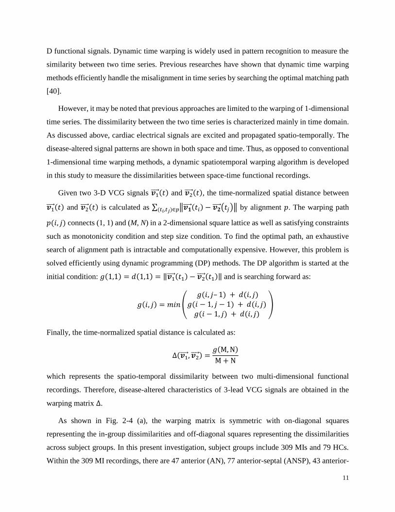
Given two 3-D VCG signals 𝒗1⃗⃗⃗⃗ (𝑡) and 𝒗2⃗⃗⃗⃗ (𝑡), the time-normalized spatial distance between
𝒗1⃗⃗⃗⃗ (𝑡) and 𝒗2⃗⃗⃗⃗ (𝑡) is calculated as ∑ ‖𝒗𝟏⃗⃗⃗⃗ (𝑡𝑖) − 𝒗𝟐⃗⃗⃗⃗ (𝑡𝑗)‖(𝑡𝑖,𝑡𝑗)∈𝑝 by alignment 𝑝. The warping path
𝑝(𝑖, 𝑗) connects (1, 1) and (M, N) in a 2-dimensional square lattice as well as satisfying constraints
such as monotonicity condition and step size condition. To find the optimal path, an exhaustive
search of alignment path is intractable and computationally expensive. However, this problem is
solved efficiently using dynamic programming (DP) methods. The DP algorithm is started at the
initial condition: 𝑔(1,1) = 𝑑(1,1) = ‖𝒗1⃗⃗⃗⃗ (𝑡1) − 𝒗2⃗⃗⃗⃗ (𝑡1)‖ and is searching forward as:
𝑔(𝑖, 𝑗) = 𝑚𝑖𝑛(
𝑔(𝑖, 𝑗– 1) + 𝑑(𝑖, 𝑗)𝑔(𝑖 − 1, 𝑗 − 1) + 𝑑(𝑖, 𝑗)
𝑔(𝑖 − 1, 𝑗) + 𝑑(𝑖, 𝑗) )
Finally, the time-normalized spatial distance is calculated as:
∆(𝒗1⃗⃗⃗⃗ , 𝒗2⃗⃗⃗⃗ ) =𝑔(M,N)
M + N
which represents the spatio-temporal dissimilarity between two multi-dimensional functional
recordings. Therefore, disease-altered characteristics of 3-lead VCG signals are obtained in the
warping matrix ∆.
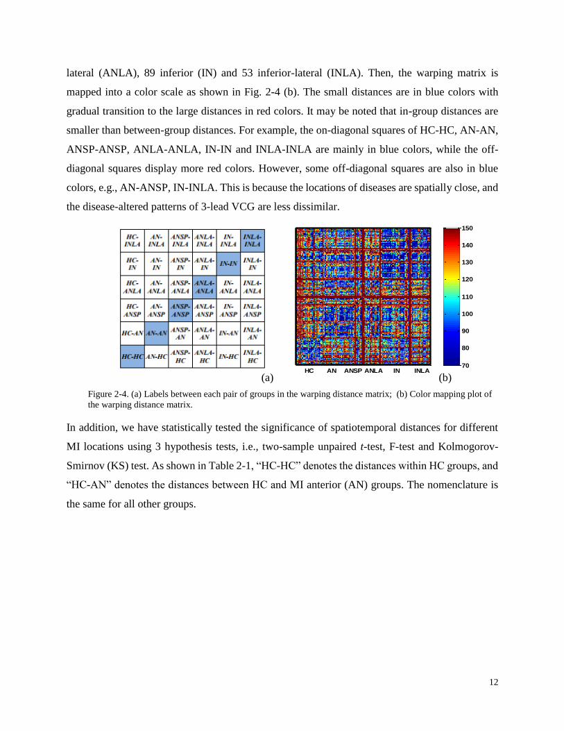
As shown in Fig. 2-4 (a), the warping matrix is symmetric with on-diagonal squares
representing the in-group dissimilarities and off-diagonal squares representing the dissimilarities
across subject groups. In this present investigation, subject groups include 309 MIs and 79 HCs.
Within the 309 MI recordings, there are 47 anterior (AN), 77 anterior-septal (ANSP), 43 anterior-
12
lateral (ANLA), 89 inferior (IN) and 53 inferior-lateral (INLA). Then, the warping matrix is
mapped into a color scale as shown in Fig. 2-4 (b). The small distances are in blue colors with
gradual transition to the large distances in red colors. It may be noted that in-group distances are
smaller than between-group distances. For example, the on-diagonal squares of HC-HC, AN-AN,
ANSP-ANSP, ANLA-ANLA, IN-IN and INLA-INLA are mainly in blue colors, while the off-
diagonal squares display more red colors. However, some off-diagonal squares are also in blue
colors, e.g., AN-ANSP, IN-INLA. This is because the locations of diseases are spatially close, and
the disease-altered patterns of 3-lead VCG are less dissimilar.
In addition, we have statistically tested the significance of spatiotemporal distances for different
MI locations using 3 hypothesis tests, i.e., two-sample unpaired t-test, F-test and Kolmogorov-
Smirnov (KS) test. As shown in Table 2-1, “HC-HC” denotes the distances within HC groups, and
“HC-AN” denotes the distances between HC and MI anterior (AN) groups. The nomenclature is
the same for all other groups.
Figure 2-4. (a) Labels between each pair of groups in the warping distance matrix; (b) Color mapping plot of
the warping distance matrix.
(a) (b)
HC AN ANSP ANLA IN INLA70
80
90
100
110
120
130
140
150

13
First, the central tendency of spatiotemporal distances is tested for different MI location with
2-sample t-test. Let 𝜇𝑖 and 𝜇𝑗denote the means of ith and jth groups, the hypotheses of t-test are:
𝐻0: 𝜇𝑖 = 𝜇𝑗 & 𝐻1: 𝜇𝑖 ≠ 𝜇𝑗
For each pair of groups, the t-test statistic is compared with critical value given by
𝑡𝛼 2⁄ , 𝑛1+ 𝑛2−2 , where 𝑛1and 𝑛2 are the number of independent observations in the corresponding
group and 𝛼 = 0.05. If |𝑡0|>𝑡𝛼 2⁄ , 𝑛1+ 𝑛2−2 , the null hypothesis 𝐻0 will be rejected and the mean
values of two groups are declared to be different at significant level of 0.05. Statistically significant
groups are marked as red colors in Table 1-1. It may be noted that the distances within HC group
are significantly different from MI groups (i.e., AN, ANSP, ANLA, IN and INLA) in terms of
mean values. It is also found that MI-anterior (AN) and MI-inferior (IN) are statistically significant
in the mean values of spatiotemporal distances.
Second, the dispersion of spatiotemporal distances is tested for different MI location with 2-
sample F-test. Let 𝜎𝑖2 and 𝜎𝑗
2 denote the variances of ith and jth groups, the hypotheses of F-test
are:
𝐻0: 𝜎𝑖2 = 𝜎𝑗
2 & 𝐻1: 𝜎𝑖2 ≠ 𝜎𝑗
2
The test statistics are compared with critical values 𝐹𝛼 2⁄ , 𝑛1−1, 𝑛2−1 and 𝐹1−𝛼 2⁄ , 𝑛1−1, 𝑛2−1 .
Here, 𝑛1and 𝑛2 are the number of independent observations in corresponding groups and the
significant level 𝛼 = 0.05. If 𝐹0 > 𝐹𝛼 2⁄ , 𝑛1−1, 𝑛2−1 or 𝐹0 < 𝐹1−𝛼 2⁄ , 𝑛1−1, 𝑛2−1 , the null hypothesis
𝐻0 will be rejected at significant level of 0.05 and there are significant differences in the variances
of spatiotemporal distances for two groups. As shown in Table 2-2, the statistics and critical values
Table 2-1. Two Sample t-Test for Testing the Mean of Spatiotemporal Distances at
Different MI Locations
Group HC-HC vs.
HC-AN
HC-HC vs.
HC-ANSP
HC-HC vs.
HC-ANLA HC-HC vs. HC-IN
HC-HC vs.
HC-INLA
t0 -3.55 -4.79 -4.40 -2.58 -2.74
t crit. 1.98 1.98 1.98 1.97 1.98
Group AN-AN vs.
AN-ANSP
AN-AN vs.
AN-ANLA
AN-AN vs.
AN-IN
AN-AN vs.
AN-INLA
ANSP-ANSP vs.
ANSP-ANLA
t0 -1.96 -1.27 -2.37 -1.90 -0.01
t crit. 1.98 1.99 1.98 1.98 1.98
Group ANSP-ANSP vs.
ANSP-IN
ANSP-ANSP vs.
ANSP-INLA
ANLA-ANLA vs.
ANLA-IN
ANLA-ANLA vs.
ANLA-INLA
IN-IN vs. IN-
INLA
t0 -0.54 0.02 -1.62 -1.11 0.35
t crit. 1.97 1.98 1.98 1.99 1.98

14
of significant groups are marked in red colors. The variances within the HC group are significantly
different from MI-anterior-septal (ANSP) and MI-inferior (IN). In addition, the variance of
spatiotemporal distances within MI-anterior (AN) is different from the distances between MI-
anterior (AN) and MI-anterior-septal (ANSP). The variances of MI-inferior-lateral (INLA) are
significantly different from another two groups, i.e., MI-anterior-lateral (ANLA) and MI-inferior
(IN).
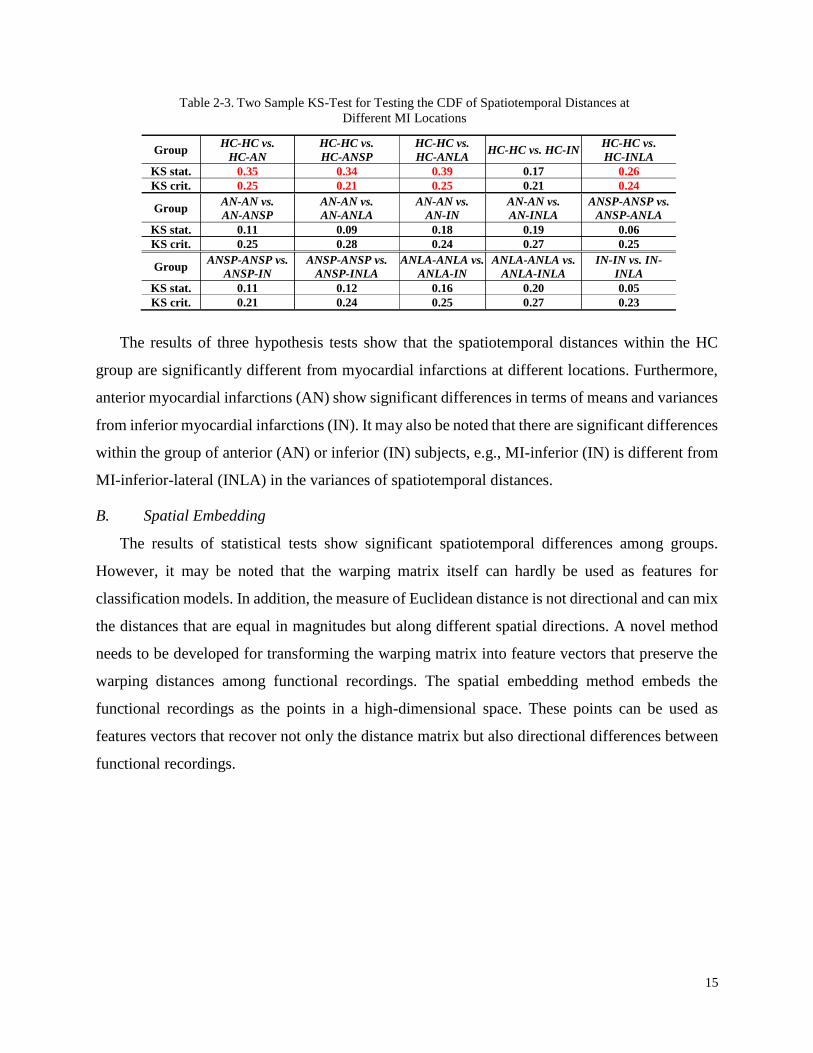
Third, two-sample KS test is utilized to test the differences in cumulative distribution function
(CDF) for MIs at various locations. Let 𝐹𝑖(𝑥)and 𝐹𝑗(𝑥) denote cumulative distribution functions
of the ith and jth groups respectively and the hypotheses of KS test are given as:
𝐻0: 𝐹𝑖(𝑥) = 𝐹𝑗(𝑥) & 𝐻1: 𝐹𝑖(𝑥) ≠ 𝐹𝑗(𝑥)
The test statistics (KS stat.) and critical values (KS crit.) are shown in the Table 2-3. The KS test
statistic is compared with the corresponding critical value given by 𝑐𝛼√𝑛1+𝑛2
𝑛1𝑛2, where n1 and n2
are the number of independent observations in corresponding groups, the significant level is 𝛼 =
0.05, and 𝑐𝛼is approximated as 1.36. If the KS statistic is greater than the critical value, the null
hypothesis 𝐻0 will be rejected and the cumulative distribution functions of two groups are declared
to be different at significant level of 0.05. As shown in Table 2-3, four significant groups are
highlighted in red colors. It may be noted that, the cumulative distribution function of HC group
is significantly different with MI-anterior (AN), MI-anterior-lateral (ANLA), MI-anterior-septal
(ANSP) and MI-inferior-lateral (INLA).
Table 2-2. Two Sample F-Test for Testing the Variance of Spatiotemporal Distances at
Different MI Locations
Group HC-HC vs.
HC-AN
HC-HC vs.
HC-ANSP
HC-HC vs.
HC-ANLA HC-HC vs. HC-IN
HC-HC vs.
HC-INLA
F0 1.17 2.10 1.22 1.57 1.06
F crit. 1.71 1.56 1.74 1.53 1.67
Group AN-AN vs.
AN-ANSP
AN-AN vs.
AN-ANLA
AN-AN vs.
AN-IN
AN-AN vs.
AN-INLA
ANSP-ANSP vs.
ANSP-ANLA
F0 2.02 1.11 1.21 1.63 1.33
F crit. 1.65 1.82 1.63 1.75 1.75
Group ANSP-ANSP vs.
ANSP-IN
ANSP-ANSP vs.
ANSP-INLA
ANLA-ANLA vs.
ANLA-IN
ANLA-ANLA vs.
ANLA-INLA
IN-IN vs. IN-
INLA
F0 1.14 1.45 1.11 1.91 1.71
F crit. 1.54 1.67 1.65 1.77 1.65
15
The results of three hypothesis tests show that the spatiotemporal distances within the HC
group are significantly different from myocardial infarctions at different locations. Furthermore,
anterior myocardial infarctions (AN) show significant differences in terms of means and variances
from inferior myocardial infarctions (IN). It may also be noted that there are significant differences
within the group of anterior (AN) or inferior (IN) subjects, e.g., MI-inferior (IN) is different from
MI-inferior-lateral (INLA) in the variances of spatiotemporal distances.
B. Spatial Embedding
The results of statistical tests show significant spatiotemporal differences among groups.
However, it may be noted that the warping matrix itself can hardly be used as features for
classification models. In addition, the measure of Euclidean distance is not directional and can mix
the distances that are equal in magnitudes but along different spatial directions. A novel method
needs to be developed for transforming the warping matrix into feature vectors that preserve the
warping distances among functional recordings. The spatial embedding method embeds the
functional recordings as the points in a high-dimensional space. These points can be used as
features vectors that recover not only the distance matrix but also directional differences between
functional recordings.
Table 2-3. Two Sample KS-Test for Testing the CDF of Spatiotemporal Distances at
Different MI Locations
Group HC-HC vs.
HC-AN
HC-HC vs.
HC-ANSP
HC-HC vs.
HC-ANLA HC-HC vs. HC-IN
HC-HC vs.
HC-INLA
KS stat. 0.35 0.34 0.39 0.17 0.26
KS crit. 0.25 0.21 0.25 0.21 0.24
Group AN-AN vs.
AN-ANSP
AN-AN vs.
AN-ANLA
AN-AN vs.
AN-IN
AN-AN vs.
AN-INLA
ANSP-ANSP vs.
ANSP-ANLA
KS stat. 0.11 0.09 0.18 0.19 0.06
KS crit. 0.25 0.28 0.24 0.27 0.25
Group ANSP-ANSP vs.
ANSP-IN
ANSP-ANSP vs.
ANSP-INLA
ANLA-ANLA vs.
ANLA-IN
ANLA-ANLA vs.
ANLA-INLA
IN-IN vs. IN-
INLA
KS stat. 0.11 0.12 0.16 0.20 0.05
KS crit. 0.21 0.24 0.25 0.27 0.23
16
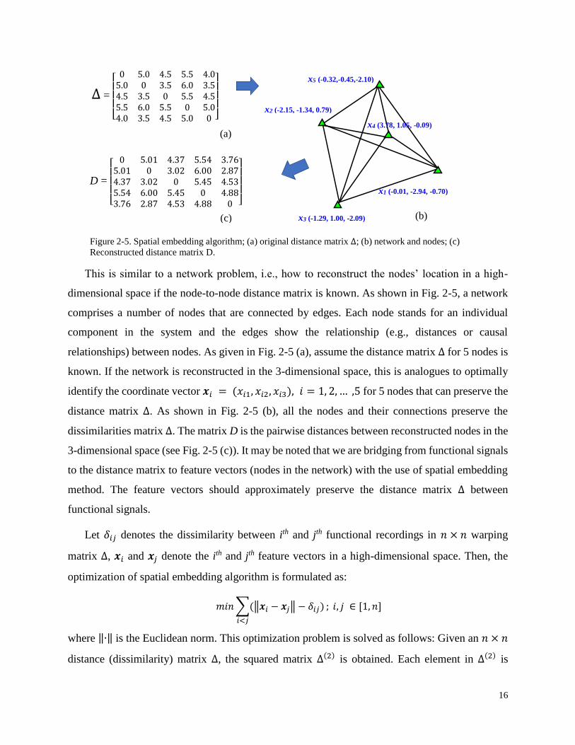
This is similar to a network problem, i.e., how to reconstruct the nodes’ location in a high-
dimensional space if the node-to-node distance matrix is known. As shown in Fig. 2-5, a network
comprises a number of nodes that are connected by edges. Each node stands for an individual
component in the system and the edges show the relationship (e.g., distances or causal
relationships) between nodes. As given in Fig. 2-5 (a), assume the distance matrix ∆ for 5 nodes is
known. If the network is reconstructed in the 3-dimensional space, this is analogues to optimally
identify the coordinate vector 𝒙𝑖 = (𝑥𝑖1, 𝑥𝑖2, 𝑥𝑖3), 𝑖 = 1, 2, … ,5 for 5 nodes that can preserve the
distance matrix ∆. As shown in Fig. 2-5 (b), all the nodes and their connections preserve the
dissimilarities matrix ∆. The matrix D is the pairwise distances between reconstructed nodes in the
3-dimensional space (see Fig. 2-5 (c)). It may be noted that we are bridging from functional signals
to the distance matrix to feature vectors (nodes in the network) with the use of spatial embedding
method. The feature vectors should approximately preserve the distance matrix ∆ between
functional signals.
Let 𝛿𝑖𝑗 denotes the dissimilarity between ith and jth functional recordings in 𝑛 × 𝑛 warping
matrix ∆, 𝒙𝑖 and 𝒙𝑗 denote the ith and jth feature vectors in a high-dimensional space. Then, the
optimization of spatial embedding algorithm is formulated as:
𝑚𝑖𝑛 ∑(‖𝒙𝑖 − 𝒙𝑗‖ − 𝛿𝑖𝑗)
𝑖<𝑗
; 𝑖, 𝑗 ∈ [1, 𝑛]
where ‖∙‖ is the Euclidean norm. This optimization problem is solved as follows: Given an 𝑛 × 𝑛
distance (dissimilarity) matrix ∆, the squared matrix ∆(2) is obtained. Each element in ∆(2) is
∆ =
ۏێێێۍ0 5.0 4.5 5.5 4.0
5.0 0 3.5 6.0 3.54.5 3.5 0 5.5 4.55.5 6.0 5.5 0 5.04.0 3.5 4.5 5.0 0 ے
ۑۑۑې
D =
ۏێێێۍ
0 5.01 4.37 5.54 3.765.01 0 3.02 6.00 2.874.37 3.02 0 5.45 4.535.54 6.00 5.45 0 4.883.76 2.87 4.53 4.88 0 ے
ۑۑۑې
(a)
(b) (c)
Figure 2-5. Spatial embedding algorithm; (a) original distance matrix ∆; (b) network and nodes; (c)
Reconstructed distance matrix D.
x5 (-0.32,-0.45,-2.10)
x2 (-2.15, -1.34, 0.79) x4 (3.78, 1.05, -0.09)
x3 (-1.29, 1.00, -2.09)
x1 (-0.01, -2.94, -0.70)
17
(𝛿𝑖𝑗)2, i.e., the squares of 𝛿𝑖𝑗 in the matrix ∆. Secondly, a Gram matrix B is constructed as: B =
−1
2𝐻∆(2)𝐻, where the centering matrix H = 𝐼 − 𝑛−1𝟏𝟏𝑇 and 1 is a column vector with n ones.
The matrix B is decomposed as: B = 𝑉𝛬𝑉𝑇, where V = [v1, v2, ..., vn] is a matrix of eigenvectors
and 𝛬 = diag(𝜆1, 𝜆2, … , 𝜆𝑛) is a diagonal matrix of eigenvalues. Then, the Gram matrix B is
rewritten as: 𝐵 = 𝑉√𝛬√𝛬𝑉𝑇. Therefore, feature vectors will be obtained as: 𝑋 = 𝑉√𝛬.
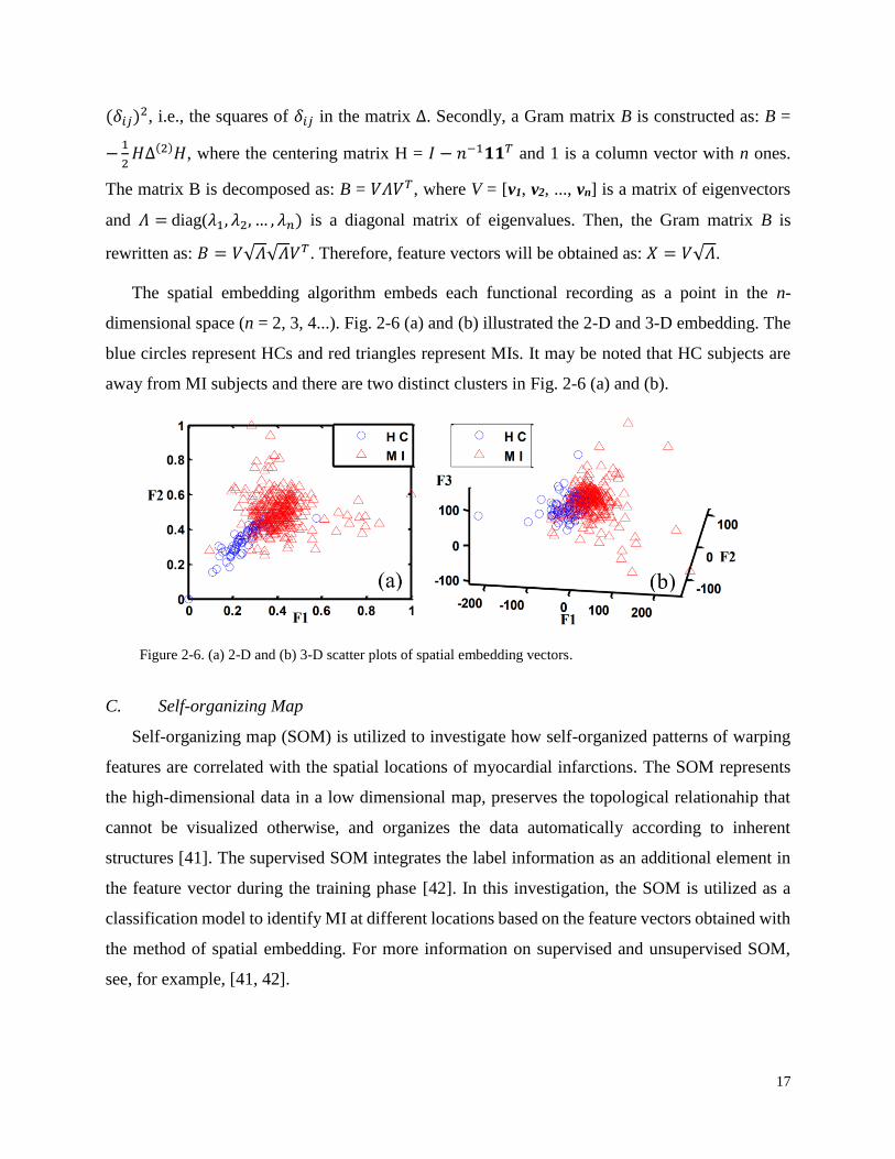
The spatial embedding algorithm embeds each functional recording as a point in the n-
dimensional space (n = 2, 3, 4...). Fig. 2-6 (a) and (b) illustrated the 2-D and 3-D embedding. The
blue circles represent HCs and red triangles represent MIs. It may be noted that HC subjects are
away from MI subjects and there are two distinct clusters in Fig. 2-6 (a) and (b).
C. Self-organizing Map
Self-organizing map (SOM) is utilized to investigate how self-organized patterns of warping
features are correlated with the spatial locations of myocardial infarctions. The SOM represents
the high-dimensional data in a low dimensional map, preserves the topological relationahip that
cannot be visualized otherwise, and organizes the data automatically according to inherent
structures [41]. The supervised SOM integrates the label information as an additional element in
the feature vector during the training phase [42]. In this investigation, the SOM is utilized as a
classification model to identify MI at different locations based on the feature vectors obtained with
the method of spatial embedding. For more information on supervised and unsupervised SOM,
see, for example, [41, 42].
Figure 2-6. (a) 2-D and (b) 3-D scatter plots of spatial embedding vectors.
18
2.3. Materials and Experimental Results
In this investigation, 3-lead VCG recordings from 388 subjects (309 MIs and 79 HCs) available
in the PTB Database of PhysioNet [10] are analyzed to evaluate the performance of developed
research methodologies. The VCG signals were digitized at 1 kHz sampling rate with a 16-bit
resolution over a range of ±16.384 mV. Within the 309 MI recordings, there are 47 anterior (AN),
77 anterior-septal (ANSP), 43 anterior-lateral (ANLA), 89 inferior (IN) and 53 inferior-lateral
(INLA). To optimize the design of research methodology, we have conducted experiments to
address the following questions:
1) The influence of embedding dimension: As the embedding dimension increases, the warping
dissimilarities between functional recordings are better preserved. However, a higher
embedding dimension will increase the model complexity and introduce “curse of
dimensionality” problem. A lower embedding dimension may not fully preserve the distance
relationships of functional recordings. In this study, a cost function is defined to represent the
performance of each embedding dimension. Experiments are conducted to investigate how the
performance will vary as the embedding dimension increases.
2) The influence of neuron map size: The classification performance of SOM can be influenced
by the map size. The larger the map size, the better performance can be achieved. However, a
large number of neurons will result in “overfitting” problems. In this study, experiments are
conducted for selecting optimal neuron map size.
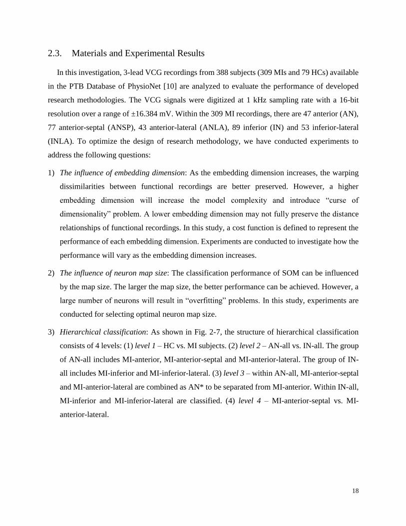
3) Hierarchical classification: As shown in Fig. 2-7, the structure of hierarchical classification
consists of 4 levels: (1) level 1 – HC vs. MI subjects. (2) level 2 – AN-all vs. IN-all. The group
of AN-all includes MI-anterior, MI-anterior-septal and MI-anterior-lateral. The group of IN-
all includes MI-inferior and MI-inferior-lateral. (3) level 3 – within AN-all, MI-anterior-septal
and MI-anterior-lateral are combined as AN* to be separated from MI-anterior. Within IN-all,
MI-inferior and MI-inferior-lateral are classified. (4) level 4 – MI-anterior-septal vs. MI-
anterior-lateral.
19
In addition, K-fold cross validation (i.e., K = 4 in this study) is used to estimate the performance
of classification models and prevent the “overfitting” problem. Three statistics, i.e., correct rate
(CR), sensitivity (SEN) and specificity (SPEC), are used as model performance metrics.
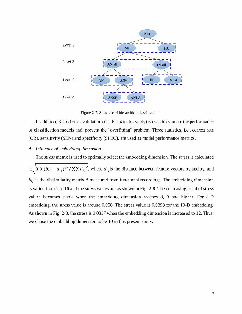
A. Influence of embedding dimension
The stress metric is used to optimally select the embedding dimension. The stress is calculated
as√∑∑(𝛿𝑖𝑗 − 𝑑𝑖𝑗)2)/∑∑𝑑𝑖𝑗
2, where 𝑑𝑖𝑗is the distance between feature vectors 𝒙𝑖 and 𝒙𝑗, and
𝛿𝑖𝑗 is the dissimilarity matrix ∆ measured from functional recordings. The embedding dimension
is varied from 1 to 16 and the stress values are as shown in Fig. 2-8. The decreasing trend of stress
values becomes stable when the embedding dimension reaches 8, 9 and higher. For 8-D
embedding, the stress value is around 0.058. The stress value is 0.0393 for the 10-D embedding.
As shown in Fig. 2-8, the stress is 0.0337 when the embedding dimension is increased to 12. Thus,
we chose the embedding dimension to be 10 in this present study.
Level 1
Figure 2-7. Structure of hierarchical classification
ALL
MI HC
AN-all IN-all
AN AN* IN INLA
ANSP ANLA
Level 2
Level 3
Level 4
20
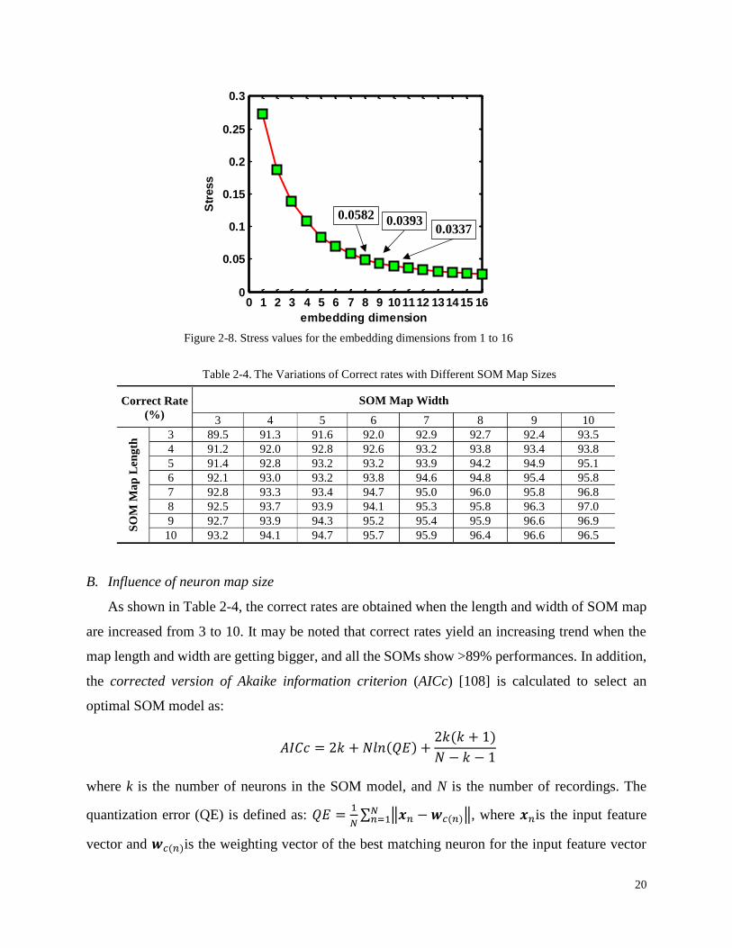
B. Influence of neuron map size
As shown in Table 2-4, the correct rates are obtained when the length and width of SOM map
are increased from 3 to 10. It may be noted that correct rates yield an increasing trend when the
map length and width are getting bigger, and all the SOMs show >89% performances. In addition,
the corrected version of Akaike information criterion (AICc) [108] is calculated to select an
optimal SOM model as:
𝐴𝐼𝐶𝑐 = 2𝑘 + 𝑁𝑙𝑛(𝑄𝐸) +2𝑘(𝑘 + 1)
𝑁 − 𝑘 − 1
where k is the number of neurons in the SOM model, and N is the number of recordings. The
quantization error (QE) is defined as: 𝑄𝐸 =1
𝑁∑ ‖𝒙𝑛 − 𝒘𝑐(𝑛)‖
𝑁𝑛=1 , where 𝒙𝑛is the input feature
vector and 𝒘𝑐(𝑛)is the weighting vector of the best matching neuron for the input feature vector
Figure 2-8. Stress values for the embedding dimensions from 1 to 16
0 1 2 3 4 5 6 7 8 9 101112 131415 160
0.05
0.1
0.15
0.2
0.25
0.3
embedding dimension
Str
ess
0.0337 0.0393 0.0582
Table 2-4. The Variations of Correct rates with Different SOM Map Sizes
Correct Rate
(%)
SOM Map Width
3 4 5 6 7 8 9 10
SO
M M
ap
Len
gth
3 89.5 91.3 91.6 92.0 92.9 92.7 92.4 93.5
4 91.2 92.0 92.8 92.6 93.2 93.8 93.4 93.8
5 91.4 92.8 93.2 93.2 93.9 94.2 94.9 95.1
6 92.1 93.0 93.2 93.8 94.6 94.8 95.4 95.8
7 92.8 93.3 93.4 94.7 95.0 96.0 95.8 96.8
8 92.5 93.7 93.9 94.1 95.3 95.8 96.3 97.0
9 92.7 93.9 94.3 95.2 95.4 95.9 96.6 96.9
10 93.2 94.1 94.7 95.7 95.9 96.4 96.6 96.5
21
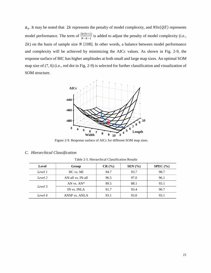
𝒙𝑛. It may be noted that 2𝑘 represents the penalty of model complexity, and 𝑁𝑙𝑛(𝑄𝐸) represents
model performance. The term of 2𝑘(𝑘+1)
𝑁−𝑘−1 is added to adjust the penalty of model complexity (i.e.,
2𝑘) on the basis of sample size 𝑁 [108]. In other words, a balance between model performance
and complexity will be achieved by minimizing the AICc values. As shown in Fig. 2-9, the
response surface of BIC has higher amplitudes at both small and large map sizes. An optimal SOM
map size of (7, 6) (i.e., red dot in Fig. 2-9) is selected for further classification and visualization of
SOM structure.
C. Hierarchical Classification
Figure 2-9. Response surface of AICc for different SOM map sizes.
Width
3 4 5 6 7 8 9 10 34
56
78
910-480
-460
-440
Length
AICc
Table 2-5. Hierarchical Classification Results
Level Group CR (%) SEN (%) SPEC (%)
Level 1 HC vs. MI 94.7 93.7 98.7
Level 2 AN-all vs. IN-all 96.5 97.0 96.1
Level 3 AN vs. AN* 89.5 88.1 93.1
IN vs. INLA 91.7 93.4 90.7
Level 4 ANSP vs. ANLA 93.1 93.0 93.1
22
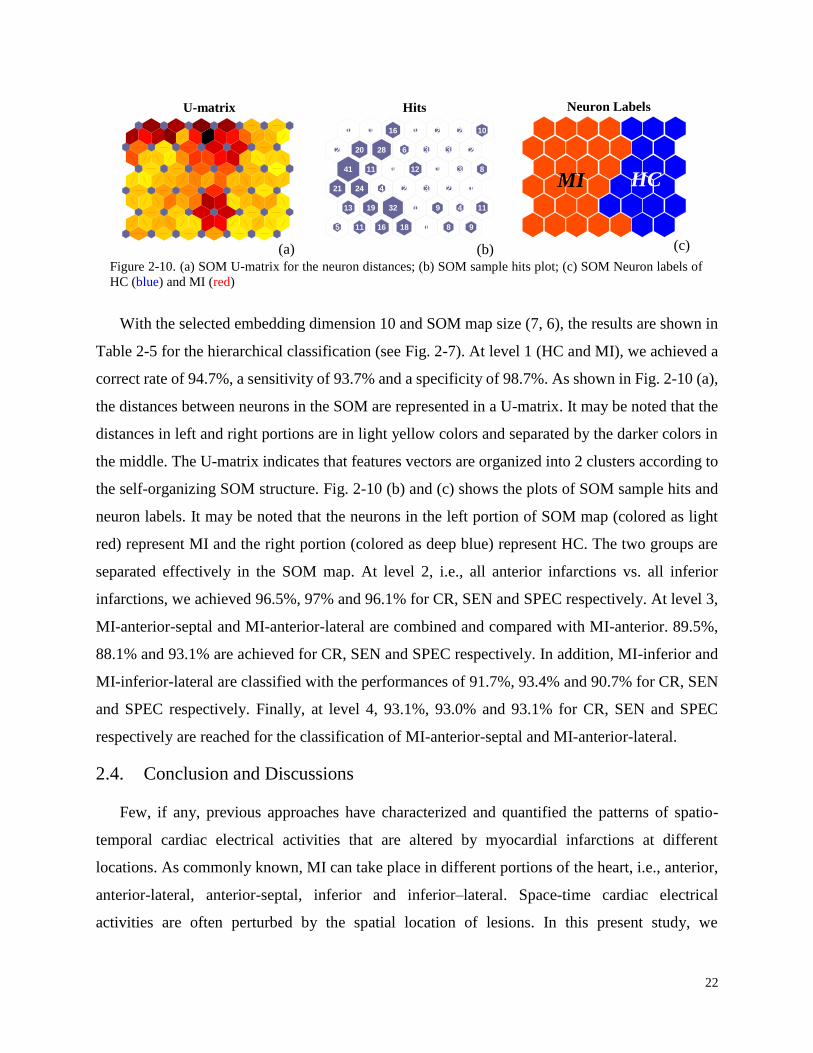
With the selected embedding dimension 10 and SOM map size (7, 6), the results are shown in
Table 2-5 for the hierarchical classification (see Fig. 2-7). At level 1 (HC and MI), we achieved a
correct rate of 94.7%, a sensitivity of 93.7% and a specificity of 98.7%. As shown in Fig. 2-10 (a),
the distances between neurons in the SOM are represented in a U-matrix. It may be noted that the
distances in left and right portions are in light yellow colors and separated by the darker colors in
the middle. The U-matrix indicates that features vectors are organized into 2 clusters according to
the self-organizing SOM structure. Fig. 2-10 (b) and (c) shows the plots of SOM sample hits and
neuron labels. It may be noted that the neurons in the left portion of SOM map (colored as light
red) represent MI and the right portion (colored as deep blue) represent HC. The two groups are
separated effectively in the SOM map. At level 2, i.e., all anterior infarctions vs. all inferior
infarctions, we achieved 96.5%, 97% and 96.1% for CR, SEN and SPEC respectively. At level 3,
MI-anterior-septal and MI-anterior-lateral are combined and compared with MI-anterior. 89.5%,
88.1% and 93.1% are achieved for CR, SEN and SPEC respectively. In addition, MI-inferior and
MI-inferior-lateral are classified with the performances of 91.7%, 93.4% and 90.7% for CR, SEN
and SPEC respectively. Finally, at level 4, 93.1%, 93.0% and 93.1% for CR, SEN and SPEC
respectively are reached for the classification of MI-anterior-septal and MI-anterior-lateral.
2.4. Conclusion and Discussions
Few, if any, previous approaches have characterized and quantified the patterns of spatio-
temporal cardiac electrical activities that are altered by myocardial infarctions at different
locations. As commonly known, MI can take place in different portions of the heart, i.e., anterior,
anterior-lateral, anterior-septal, inferior and inferior–lateral. Space-time cardiac electrical
activities are often perturbed by the spatial location of lesions. In this present study, we
1 2 3 4 5 6 7
1
2
3
4
5
6
SOM Neighbor Weight Distances
1 2 3 4 5 6 7
1
2
3
4
5
6
5 11 16 18 1 8 9
13 19 32 1 9 4 11
21 24 4 2 3 2 1
41 11 1 12 1 3 8
2 20 28 6 3 3 2
1 1 16 1 2 2 10
Hits
1 2 3 4 5 6 7
1
2
3
4
5
6
SOM Topology
U-matrix Hits Neuron Labels
MI HC
(a) (b) (c)
Figure 2-10. (a) SOM U-matrix for the neuron distances; (b) SOM sample hits plot; (c) SOM Neuron labels of
HC (blue) and MI (red)

23
characterized the disease-altered cardiac electrical activities in the 3-lead VCG. However, the
VCG signals are often misaligned due to discrete sampling and phase shift. A novel method of
dynamic spatio-temporal warping is designed to overcome the misalignment problem and measure
the spatiotemporal distances between VCG signals. The hypothesis tests show that there are
significant spatio-temporal differences between the subject groups in the dissimilarity matrix.
Furthermore, functional recordings are optimally embedded as points in a high-dimensional space
that preserve the warping distance matrix. Finally, the proposed multi-class classification models
yield superior classification results (>94.7%) in the first 2 levels. At levels 3 and 4, because MIs
are spatially close to each other, disease-altered cardiac electrical activities are similar, thereby
achieving a relatively low accuracy (>89.5%). The developed methodologies facilitate the
understanding of disease-altered spatio-temporal patterns in the complex cardiac systems.

24
Chapter 3: Dynamic Network Modeling and Control of in-situ Image
Profiles from Ultraprecision Machining and Biomanufacturing
Processes2
Abstract
In modern industries, advanced imaging technology has been more and more invested to cope
with the ever-increasing complexity of systems, improve the visibility of information, and enhance
operational quality and integrity. As a result, large amounts of imaging data are readily available.
This presents great challenges on the state-of-the-art practices in process monitoring and quality
control. Conventional statistical process control (SPC) focuses on key characteristics of the product
or process, and is rather limited to handle complex structures of high-dimensional imaging data.
New SPC methods and tools are urgently needed to extract useful information from in-situ image
profiles for process monitoring and quality control. In this study, we developed a novel dynamic
network scheme to represent, model and control of time-varying image profiles. Potts model
Hamiltonian approach is introduced to characterize community patterns and organizational
behaviors in the dynamic network. Further, new statistics are extracted from network communities
to characterize and quantify dynamic structures of image profiles. Finally, we design and develop
a new control chart, namely network generalized likelihood ratio chart (NGLR), to detect the change
point of the underlying dynamics of complex processes. The proposed methodology is implemented
and evaluated for real-world applications in ultra-precision machining and biomanufacturing
processes. Experimental results show that the proposed approach effectively characterize and
monitor the variations in complex structures of time-varying image data. The new dynamic network
SPC method is shown to have strong potentials for general applications in a diverse set of domains
with in-situ imaging data.
2 This Chapter has been published in the Journal of Quality and Reliability Engineering International
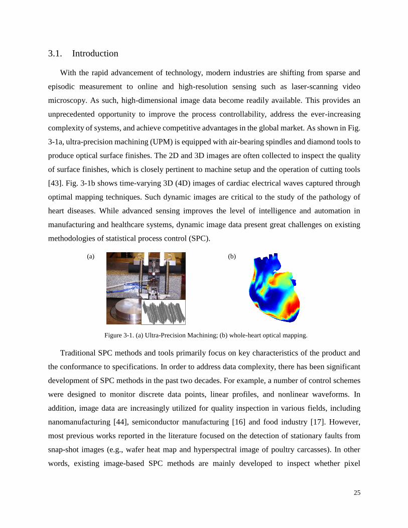
25
3.1. Introduction
With the rapid advancement of technology, modern industries are shifting from sparse and
episodic measurement to online and high-resolution sensing such as laser-scanning video
microscopy. As such, high-dimensional image data become readily available. This provides an
unprecedented opportunity to improve the process controllability, address the ever-increasing
complexity of systems, and achieve competitive advantages in the global market. As shown in Fig.
3-1a, ultra-precision machining (UPM) is equipped with air-bearing spindles and diamond tools to
produce optical surface finishes. The 2D and 3D images are often collected to inspect the quality
of surface finishes, which is closely pertinent to machine setup and the operation of cutting tools
[43]. Fig. 3-1b shows time-varying 3D (4D) images of cardiac electrical waves captured through
optimal mapping techniques. Such dynamic images are critical to the study of the pathology of
heart diseases. While advanced sensing improves the level of intelligence and automation in
manufacturing and healthcare systems, dynamic image data present great challenges on existing
methodologies of statistical process control (SPC).
Traditional SPC methods and tools primarily focus on key characteristics of the product and
the conformance to specifications. In order to address data complexity, there has been significant
development of SPC methods in the past two decades. For example, a number of control schemes
were designed to monitor discrete data points, linear profiles, and nonlinear waveforms. In
addition, image data are increasingly utilized for quality inspection in various fields, including
nanomanufacturing [44], semiconductor manufacturing [16] and food industry [17]. However,
most previous works reported in the literature focused on the detection of stationary faults from
snap-shot images (e.g., wafer heat map and hyperspectral image of poultry carcasses). In other
words, existing image-based SPC methods are mainly developed to inspect whether pixel
Figure 3-1. (a) Ultra-Precision Machining; (b) whole-heart optical mapping.
(a) (b)
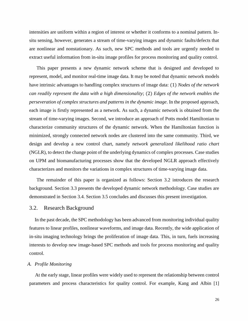
26
intensities are uniform within a region of interest or whether it conforms to a nominal pattern. In-
situ sensing, however, generates a stream of time-varying images and dynamic faults/defects that
are nonlinear and nonstationary. As such, new SPC methods and tools are urgently needed to
extract useful information from in-situ image profiles for process monitoring and quality control.
This paper presents a new dynamic network scheme that is designed and developed to
represent, model, and monitor real-time image data. It may be noted that dynamic network models
have intrinsic advantages to handling complex structures of image data: (1) Nodes of the network
can readily represent the data with a high dimensionality; (2) Edges of the network enables the
perseveration of complex structures and patterns in the dynamic image. In the proposed approach,
each image is firstly represented as a network. As such, a dynamic network is obtained from the
stream of time-varying images. Second, we introduce an approach of Potts model Hamiltonian to
characterize community structures of the dynamic network. When the Hamiltonian function is
minimized, strongly connected network nodes are clustered into the same community. Third, we
design and develop a new control chart, namely network generalized likelihood ratio chart
(NGLR), to detect the change point of the underlying dynamics of complex processes. Case studies
on UPM and biomanufacturing processes show that the developed NGLR approach effectively
characterizes and monitors the variations in complex structures of time-varying image data.
The remainder of this paper is organized as follows: Section 3.2 introduces the research
background. Section 3.3 presents the developed dynamic network methodology. Case studies are
demonstrated in Section 3.4. Section 3.5 concludes and discusses this present investigation.
3.2. Research Background
In the past decade, the SPC methodology has been advanced from monitoring individual quality
features to linear profiles, nonlinear waveforms, and image data. Recently, the wide application of
in-situ imaging technology brings the proliferation of image data. This, in turn, fuels increasing
interests to develop new image-based SPC methods and tools for process monitoring and quality
control.
A. Profile Monitoring
At the early stage, linear profiles were widely used to represent the relationship between control
parameters and process characteristics for quality control. For example, Kang and Albin [1]
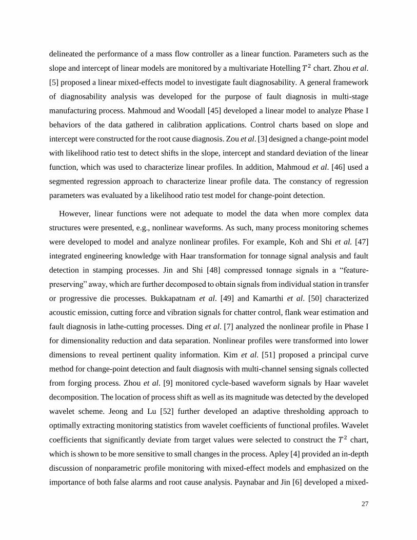
27
delineated the performance of a mass flow controller as a linear function. Parameters such as the
slope and intercept of linear models are monitored by a multivariate Hotelling 𝑇2 chart. Zhou et al.
[5] proposed a linear mixed-effects model to investigate fault diagnosability. A general framework
of diagnosability analysis was developed for the purpose of fault diagnosis in multi-stage
manufacturing process. Mahmoud and Woodall [45] developed a linear model to analyze Phase I
behaviors of the data gathered in calibration applications. Control charts based on slope and
intercept were constructed for the root cause diagnosis. Zou et al. [3] designed a change-point model
with likelihood ratio test to detect shifts in the slope, intercept and standard deviation of the linear
function, which was used to characterize linear profiles. In addition, Mahmoud et al. [46] used a
segmented regression approach to characterize linear profile data. The constancy of regression
parameters was evaluated by a likelihood ratio test model for change-point detection.
However, linear functions were not adequate to model the data when more complex data
structures were presented, e.g., nonlinear waveforms. As such, many process monitoring schemes
were developed to model and analyze nonlinear profiles. For example, Koh and Shi et al. [47]
integrated engineering knowledge with Haar transformation for tonnage signal analysis and fault
detection in stamping processes. Jin and Shi [48] compressed tonnage signals in a “feature-
preserving” away, which are further decomposed to obtain signals from individual station in transfer
or progressive die processes. Bukkapatnam et al. [49] and Kamarthi et al. [50] characterized
acoustic emission, cutting force and vibration signals for chatter control, flank wear estimation and
fault diagnosis in lathe-cutting processes. Ding et al. [7] analyzed the nonlinear profile in Phase I
for dimensionality reduction and data separation. Nonlinear profiles were transformed into lower
dimensions to reveal pertinent quality information. Kim et al. [51] proposed a principal curve
method for change-point detection and fault diagnosis with multi-channel sensing signals collected
from forging process. Zhou et al. [9] monitored cycle-based waveform signals by Haar wavelet
decomposition. The location of process shift as well as its magnitude was detected by the developed
wavelet scheme. Jeong and Lu [52] further developed an adaptive thresholding approach to
optimally extracting monitoring statistics from wavelet coefficients of functional profiles. Wavelet
coefficients that significantly deviate from target values were selected to construct the 𝑇2 chart,
which is shown to be more sensitive to small changes in the process. Apley [4] provided an in-depth
discussion of nonparametric profile monitoring with mixed-effect models and emphasized on the
importance of both false alarms and root cause analysis. Paynabar and Jin [6] developed a mixed-
28
effect model and used wavelet decomposition to identify within- and between-profile variations for
process monitoring. Chen and Yang [53] proposed a heterogeneous recurrence control chart for
online monitoring in nonlinear dynamic processes.
B. Image Profiles
However, existing SPC methods and tools focus on key product characteristics, linear and
nonlinear profiles instead of image profiles that are nonlinear and nonstationary. In the past few
years, the increasing availability of time-varying image profiles has attracted growing interests on
image-based SPC. For example, Du et al. [17] analyzed hyperspectral images of poultry carcasses.
A spectral band selection approach was developed to extract features for the detection of skin
tumors. Wilcox et al. [18] also investigated how to optimally select a subset of spectral bands from
hyperspectral images for the automatic monitoring of animal feed quality. Megahed et al. [20]
compared the manufactured tiles with a specific pattern and designed a generalized likelihood ratio
chart to detect the non-conforming tiles. Park et al. [44] investigated microscopic images of
nanoparticle dynamics. Morphology of nanoparticles was characterized by a multistage procedure
and then semi-automatically classify them into homogeneous groups. Yan et al. proposed to
integrate low-rank tensor decomposition with multivariate control charts for image-based process
monitoring [19]. In addition, Zhang et al. [16] measured the variations of wafer thickness from
image profiles using an additive Gaussian process model.
However, most previous studies focus on fault detection from snap-shot images in discrete-part
manufacturing. Very little has been done to model the stream of time-varying image profiles that
are highly nonlinear and nonstationary. It may be noted that faults or defects are stationary in snap-
shot images, but nonstationary in the in-situ stream of image data. There is an urgent need to design
and develop new SPC methods and tools that can extract useful information from in-situ image
profiles as well as exploit the acquired information for process monitoring and quality control.
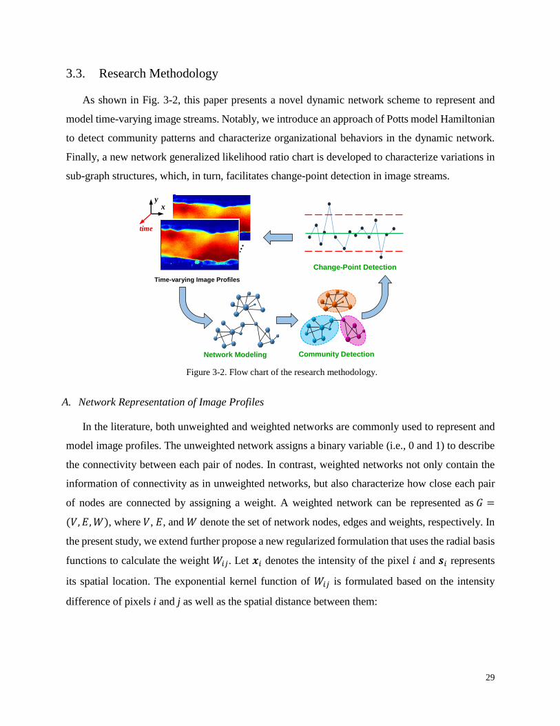
29
3.3. Research Methodology
As shown in Fig. 3-2, this paper presents a novel dynamic network scheme to represent and
model time-varying image streams. Notably, we introduce an approach of Potts model Hamiltonian
to detect community patterns and characterize organizational behaviors in the dynamic network.
Finally, a new network generalized likelihood ratio chart is developed to characterize variations in
sub-graph structures, which, in turn, facilitates change-point detection in image streams.
A. Network Representation of Image Profiles
In the literature, both unweighted and weighted networks are commonly used to represent and
model image profiles. The unweighted network assigns a binary variable (i.e., 0 and 1) to describe
the connectivity between each pair of nodes. In contrast, weighted networks not only contain the
information of connectivity as in unweighted networks, but also characterize how close each pair
of nodes are connected by assigning a weight. A weighted network can be represented as 𝐺 =
(𝑉, 𝐸,𝑊), where 𝑉, 𝐸, and 𝑊 denote the set of network nodes, edges and weights, respectively. In
the present study, we extend further propose a new regularized formulation that uses the radial basis
functions to calculate the weight 𝑊𝑖𝑗. Let 𝒙𝑖 denotes the intensity of the pixel 𝑖 and 𝒔𝑖 represents
its spatial location. The exponential kernel function of 𝑊𝑖𝑗 is formulated based on the intensity
difference of pixels i and j as well as the spatial distance between them:
Time-varying Image Profiles
time
x y
Change-Point Detection
Community Detection Network Modeling
Figure 3-2. Flow chart of the research methodology.
30
𝑊𝑖,𝑗 = exp (α ‖𝒙𝑖 − 𝒙𝑗‖ + (1 − α)‖𝒔𝑖 − 𝒔𝑗‖
2 × 𝑙2) (3.1)
where 𝑙 denotes the bandwidth of the exponential kernel. The regularization parameter α ∈ [0,1]
balances between intensity differences ‖𝒙𝑖 − 𝒙𝑗‖ and spatial distances ‖𝒔𝑖 − 𝒔𝑗‖. When α is larger,
the weight 𝑊𝑖𝑗 primarily focuses on intensity differences among pixels. Nodes i and j will be
assigned a smaller weight if their corresponding pixels share similar intensity values. When α is
smaller, the weight 𝑊𝑖𝑗 focuses more on distances between spatial locations of pixels. Hence, 𝑊𝑖𝑗
is smaller if corresponding pixels of nodes i and j are located closer to each other. Notably, Eq. (3.1)
can be readily used to cast different types of images (e.g., gray-scale and RGB) into networks. In
gray-scale image, the intensity of pixel 𝑥𝑖 is denoted by a scalar within the range [0, 255]. In RGB
image, the intensity of pixel 𝒙𝑖 is represented by a vector with 3 elements of primary colors, i.e.,
red, green, and blue.
B. Network Community Modeling and Characterization
To this end, image profiles are represented as networks, with nodes correspond to pixels and
weights preserve the relationship among pixels. Next, it is critical to detect sub-graph structures
from the network, i.e., network communities. A community is defined as a cluster of tightly
connected network nodes. The internal connectivity of network nodes within a community is
higher than their external connectivity to the remainder of the network. As the network preserves
the relationship among image pixels, each community correspondingly represents a group of pixels
that form a specific pattern in the image. Detection of network communities provides a great
opportunity to uncover organizational structures of the network for the study of interacting objects
and the relations between them. In the literature, a number of approaches were reported for the
detection of network communities. For example, Newman [54] calculated the network modularity
to quantify the connectivity among network nodes. By maximizing the modularity, densely
connected nodes tend to be clustered into the same community. Furthermore, Mankad and
Michailidis [55] applied the non-negative matrix factorization to characterize community
structures from a sequence of networks. By adding sparse and smooth constraints, the algorithm
is scalable to large networks and accommodates sudden changes in the network topology. In
addition, prior research extended the network community detection to image segmentation [56].

31
However, most previous studies focused on networks (e.g., social network [54] and biological
network [57]) and did not specifically consider the stream of imaging data. Little work has been
done on the community detection of dynamic image streams for the purpose of process quality
control.
In this study, we introduce the Potts model Hamiltonian [56] to detect communities in the
dynamic network for the modeling and analysis of time-varying image profiles. First, a “Potts
type” variable 𝑔𝑖 is assigned to each network node to label the index of its community. That is,
𝑔𝑖 = 1 when node 𝑖 belongs to the 1st community and 𝑔𝑖 ∈ [1, 𝐾] for the network with 𝐾
communities. As such, the network can be characterized by the state of “Potts type” variables of
N nodes, i.e., {𝑔𝑖}𝑖=1,…,𝑁. The network energy is then characterized by the Potts model Hamiltonian
function as:
ℋ({𝑔𝑖}𝑖=1𝑁 ) =
1
2∑ ∑ 𝑖,𝑗∈𝐶𝑘
(𝑊𝑖𝑗 − �̅�)[𝛩(�̅� − 𝑊𝑖𝑗) + 𝛾𝛩(𝑊𝑖𝑗 − �̅�)]𝛿(𝑔𝑖, 𝑔𝑗𝐾𝑘=1 ) (3.2)
Here, 𝑖, 𝑗 ∈ 𝐶𝑘 indicate nodes 𝑖 and 𝑗 belong to the same community 𝐶𝑘. 𝛩(∙) is the Heaviside
function, whose value is 0 for negative argument and 1 for positive argument. �̅� denotes the
average of all weights and 𝛿(𝑔𝑖, 𝑔𝑗) is the Kronecker delta with 𝛿(𝑔𝑖, 𝑔𝑗) = 1 if 𝑔𝑖 = 𝑔𝑗. Notably,
assigning node 𝑖 and 𝑗 into the same community will increase the network Hamiltonian when the
weight 𝑊𝑖𝑗 is small (i.e., 𝑊𝑖𝑗 > �̅�). Hence, a regularization parameter 𝛾 is introduced to penalize
the increase of network Hamiltonian. A larger 𝛾 will result in a more significant increase of
network community when node 𝑖 and 𝑗 with a large weight 𝑊𝑖𝑗 are assigned into the same
community.
It may be noted from Eq. (3.2) that if nodes 𝑖 and 𝑗 share a small weight (i.e., 𝑊𝑖𝑗 < �̅�), then
𝛩(𝑊𝑖𝑗 − �̅�) = 0. Assigning nodes 𝑖 and 𝑗 into the same community (i.e., having 𝑔𝑖 = 𝑔𝑗) will
decrease Hamiltonian ℋ by ∆ℋ = (𝑊𝑖𝑗 − �̅�). However, if node 𝑖 and 𝑗 are associated with a
large weight (i.e., 𝑊𝑖𝑗 > �̅�), then 𝛩(𝑊𝑖𝑗 − �̅�) = 1. A penalized increase of ∆ℋ = 𝛾(𝑊𝑖𝑗 − �̅�)
will incur if node 𝑖 and 𝑗 are assigned to the same community (i.e., 𝑔𝑖 = 𝑔𝑗). Therefore,
minimizing the Potts model Hamiltonian, i.e., min𝑔𝑖,𝑔𝑗ℋ({𝑔𝑖}𝑖=1
𝑁 ), 𝑠. 𝑡. 1 ≤ 𝑔𝑖 ≤ 𝐾, will reveal
the underlying structure of network communities. The optimization of Potts model Hamiltonian

32
aggregates densely connected nodes by assigning the same value to their Potts type variables,
whereas separates loosely related nodes into different communities.
However, the objective function of Potts model Hamiltonian is NP-hard to be minimized
exactly. Thus, a heuristic algorithm is introduced to extract network communities that
approximately optimizes the Potts model Hamiltonian in Eq. (3.2). As shown in Table 3-1, the order
of nodes are first randomly permuted and each node is considered as an individual community.
Further, we assign each node to its neighboring communities and calculate the change of
Hamiltonian ∆ℋ. The assignment that decreases ℋ to the largest extent will be retained. Here, a
neighboring community of one node is the community that contains nodes with stronger
connections (e.g., smaller weights) to that node. For example, all nodes 𝑗 that have weights 𝑊𝑖𝑗
less than a user-defined threshold are considered to be neighbors of node 𝑖 and communities that
nodes 𝑗 belong to are neighboring communities of node 𝑖. Assigning node 𝑖 to its neighboring
communities will reduce the computation time when the number of nodes 𝑁 is large. In addition,
we iterate through all the 𝑁 nodes to achieve the convergence of Hamiltonian ℋ. It is noteworthy
that the Potts model Hamiltonian is an unsupervised approach and the number of communities K
does not need to be fixed beforehand.
1: G - network, ℋ - network Hamiltonian, 𝑔𝑖 – community label
2: repeat
3: Random permutation of the order of nodes
4: Treat each node as a community
5: while ℋ does not converge
6: for all node i in G do
7:
Assign node i to its neighboring communities
Calculate ∆ℋ for each assignment
Choose the assignment which maximally decreases ℋ
8: end for
9: end while
10: If ℋis smaller than that obtained from last replication
11: Keep the newly obtained {𝑔𝑖}𝑖=1,…,𝑁
12: else
13: Terminate
14: end if
15: until min(ℋ) is achieved
Table 3-1. The Potts Model Hamiltonian Algorithm for Network Community Detection

33
Fig. 3-3 shows community detection results on benchmark images using Potts model
Hamiltonian. Original images from the Berkeley BSDS500 dataset [58] are shown in Fig. 3-3a.
Notably, a smaller number of communities separates the main object from the background, e.g., the
plane and building are depicted by two communities in Fig. 3-3b. On the contrary, a larger number
of communities delineates detailed information of the original image. For example, ten
communities not only characterize detailed patterns on the plane, but also depict the morphology
of clouds (see the top figure in Fig. 3-3c).
Figure 3-3. Examples of community detection using the Hamiltonian algorithm. (a) original images; (b) two
communities; (c) ten communities.
C. Multivariate Monitoring of Network Statistics
As the Hamiltonian approach favors strongly connected nodes into one community, image pixels
within each community are homogeneous. Therefore, pixel intensities within the kth community of
the image profile 𝐼(𝑖) approximately follows a normal distribution 𝑁 (𝜇𝑘(𝑖)
, 𝜎𝑘(𝑖)2
) with mean 𝜇𝑘(𝑖)
and variance 𝜎𝑘(𝑖)2
. Further, we extracted a Q-variate vector of community statistics for the 𝑖𝑡ℎimage
profile as:
𝒚(𝑖) = (�̅�1(𝑖)
, … , �̅�𝐾(𝑖)
, 𝑠1(𝑖)
, … , 𝑠𝐾(𝑖)
, 𝑛1(𝑖)
, … , 𝑛𝐾(𝑖)
)𝑇
(3.3)
where i = 1, 2,…,m is the time index of m image profiles, �̅�𝑘(𝑖)
is the sample mean of pixel
intensities, 𝑠𝑘(𝑖)
is the sample standard deviation, and 𝑛𝑘(𝑖)
is the number of pixels in the kth
community. The dimensionality of the community feature vector is 𝑄 = 3 × 𝐾.
Original images Two communities Ten communities (a) (b) (c)

34
Proposition 1: If the process is in control, 𝒚(𝑖) is approximately a multivariate normal distribution
as 𝒚(𝑖)~𝑀𝑉𝑁(𝝁0, 𝜮), where 𝝁0 and 𝜮 are in-control mean and covariance matrix of feature vectors.
The proof of Proposition 1 is given in Appendix A.
The variations of community statistics distinctly mark the emergent properties of anomalies in the
stream of images. If process shift occurs at the 𝜏𝑡ℎ image, the process mean is shifted to 𝝁1 and
𝒚(𝑖)~𝑀𝑉𝑁(𝝁1, 𝜮). As a result, the hypothesis of change-point detection is formulated as:
{𝐻0: 𝐸[𝒚(𝑖)]𝑖=1
𝜏 = 𝐸[𝒚(𝑖)]𝑖=𝜏+1𝑚 = 𝝁0
𝐻1: 𝐸[𝒚(𝑖)]𝑖=1𝜏 ≠ 𝐸[𝒚(𝑖)]𝑖=𝜏+1
𝑚 = 𝝁1
(3.4)
Furthermore, we propose a NGLR chart to monitor the multivariate vector of network
community statistics. For a stream of m image profiles, we have the data sample of (𝒚(1), 𝒚(2),
… , 𝒚(𝑖), … , 𝒚(𝑚)). Under the null hypothesis 𝐻0, all m feature vectors are from in-control
distribution and the likelihood function is:
𝐿(𝝁0) = ∏1
(2𝜋)𝑄2 |𝜮|
12
𝑚
𝑖=1
exp (−1
2(𝒚(𝑖) − 𝝁0)
𝑇𝜮−1(𝒚(𝑖) − 𝝁0)) (3.5)
Under the alternative hypothesis 𝐻1, a process shift occurs at the 𝜏𝑡ℎ image. The likelihood function
becomes:
𝐿(𝝁0, 𝝁1) = (1
(2𝜋)𝑄2 |𝜮|
12
)
𝑚
× ∏exp(−1
2(𝒚(𝑖) − 𝝁0)
𝑇𝜮−1(𝒚(𝑖) − 𝝁0))
𝜏
𝑖=1
× ∏ exp (−1
2(𝒚(𝑖) − 𝝁1)
𝑇𝜮−1(𝒚(𝑖) − 𝝁1))
𝑚
𝑖=𝜏+1
(3.6)
The process mean after the shift at the 𝜏𝑡ℎ image profile is estimated as:
�̂�𝑚,𝜏,𝒚 =1
(𝑚 − 𝜏)∑ 𝒚(𝑖)
𝑚
𝑖=𝜏+1
(3.7)
The maximum log likelihood ratio statistic is defined as:

35
𝑅𝑚,𝒚 = 𝑙𝑜𝑔𝐿(𝝁0, 𝝁1)
𝐿(𝝁0)= 𝑙𝑜𝑔
max0≤𝜏<𝑚𝐿(𝝁0, �̂�𝑚,𝜏,𝒚)
𝐿(𝝁0) (3.8)
Similar to the results of Wang and Reynolds [59], the multivariate NGLR statistic at the mth image
is computed as:
𝑅𝑚,𝒚 = max0≤𝜏<𝑚
𝑚 − 𝜏
2(�̂�𝑚,𝜏,𝒚 − 𝝁0)
𝑇𝜮−1(�̂�𝑚,𝜏,𝒚 − 𝝁0) (3.9)
If population mean 𝝁0 and covariance 𝜮 are replaced with the sample mean �̅� and sample
covariance 𝑺 estimated from the in-control data, then the NGLR statistic in Eq. (3.9) becomes:
𝑅𝑚,𝒚 = max0≤𝜏<𝑚
𝑚 − 𝜏
2(�̂�𝑚,𝜏,𝒚 − �̅�)
𝑇𝑺−1(�̂�𝑚,𝜏,𝒚 − �̅�) (3.10)
However, the computation of NGLR statistic will be expensive if we take account of all the
historical image profiles (i.e., m is large). To facilitate the online monitoring, it is common to
consider images within a sliding window, 𝑚 − 𝑤 ≤ 𝜏 < 𝑚, as opposed to 0 ≤ 𝜏 < 𝑚. Therefore,
the computation of online NGLR statistic becomes:
𝑅𝑚,𝒚 = max𝑚−𝑤≤𝜏<𝑚
𝑚 − 𝜏
2(�̂�𝑚,𝜏,𝒚 − �̅�)
𝑇𝑺−1(�̂�𝑚,𝜏,𝒚 − �̅�) (3.11)
As shown in the top portion of Fig. 3-4, each solid bar represents a Q-variate vector 𝒚(𝑖) and the
square box is a sliding window of size 𝑤 that contains feature vectors from 𝒚(𝑚−𝑤) to 𝒚(𝑚−1).
According to Eq. (3.7), �̂�𝑚,𝜏,𝒚 is process mean calculated from 𝒚(𝜏+1) to 𝒚(𝑚). Eq. (3.11) shows
that the computation is repeated in the sliding window for 𝜏 values from 𝑚 − 𝑤 to 𝑚. Finally, 𝑅𝑚,𝒚
is the maximal statistic obtained by varying 𝜏 values within the current window.
However, there are technical difficulties in the computation of NGLR statistics 𝑅𝑚,𝒚. Note that
Eq. (3.11) involves the inversion of sample covariance matrix 𝑺. If two communities share the same
distribution in pixel intensities, then 𝑺 will be singular that makes the NGLR computation
impractical. For example, two communities in Fig. 3-3 may be farther apart but correspond to the
same object (i.e., the cloud). As such, these two communities have the same distribution of pixel
intensities. The Q-variate vector 𝒚(𝑖) will have features that are very close to each other for these
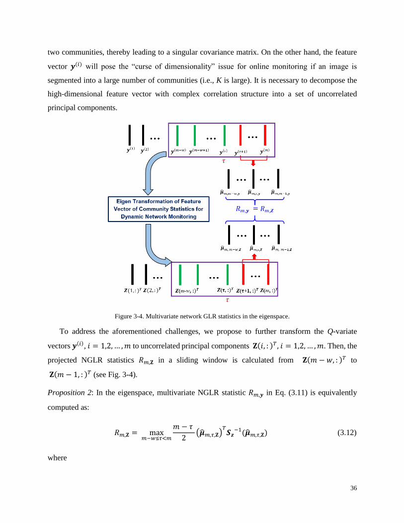
36
two communities, thereby leading to a singular covariance matrix. On the other hand, the feature
vector 𝒚(𝑖) will pose the “curse of dimensionality” issue for online monitoring if an image is
segmented into a large number of communities (i.e., K is large). It is necessary to decompose the
high-dimensional feature vector with complex correlation structure into a set of uncorrelated
principal components.
Figure 3-4. Multivariate network GLR statistics in the eigenspace.
To address the aforementioned challenges, we propose to further transform the Q-variate
vectors 𝒚(𝑖), 𝑖 = 1,2, … ,𝑚 to uncorrelated principal components 𝐙(𝑖, : )𝑇 , 𝑖 = 1,2, … ,𝑚. Then, the
projected NGLR statistics 𝑅𝑚,𝐙 in a sliding window is calculated from 𝐙(𝑚 − 𝑤, : )𝑇 to
𝐙(𝑚 − 1, : )𝑇 (see Fig. 3-4).
Proposition 2: In the eigenspace, multivariate NGLR statistic 𝑅𝑚,𝒚 in Eq. (3.11) is equivalently
computed as:
𝑅𝑚,𝐙 = max𝑚−𝑤≤𝜏<𝑚
𝑚 − 𝜏
2(�̂�𝑚,𝜏,𝐙)
𝑇𝑺𝒛
−1(�̂�𝑚,𝜏,𝐙) (3.12)
where

37
�̂�𝑚,𝜏,𝐙 =1
(𝑚 − 𝜏)∑ 𝐙(𝑖, : )𝑇
𝑚
𝑖=𝜏+1
(3.13)
and 𝐙(𝑖, : )𝑇, 𝑖 = 1,2, … ,𝑚 are principal components obtained by eigen transformation of feature
vector 𝒚(𝑖).
The proof of Proposition 2 in Appendix B.
Furthermore, a truncated 𝑚-by-𝑞 score matrix �̃� can be obtained by considering only the first
𝑑 eigen values and eigenvectors (𝑞 < 𝑄), which explains the majority of variations in the feature
matrix 𝐘. Hence, the NGLR statistic 𝑅𝑚,�̃� in the reduced dimension d becomes:
�̂�𝑚,𝜏,�̃� =1
(𝑚 − 𝜏)∑ 𝐙(𝑖, 1: 𝑞)𝑇
𝑚
𝑖=𝜏+1
(3.14)
The NGLR control chart signals when the statistic 𝑅𝑚,𝐙 falls beyond the control limits. In order
to achieve a desired in-control performance, the control limit is obtained by simulating large number
of in-control profiles and then estimate the distribution of NGLR statistics. Average run length
(ALR) is also used to measure in-control performance (type I error) of control limits. Case studies
to evaluate performances of our developed NGLR algorithm will be described in Section 3.4.
3.4. Experiments and Results
In this present paper, we implement and evaluate the proposed methodology for real-world
applications in both biomanufacturing process and UPM. The laser-scanning video microscopy
captures in-vivo images of living cells during the synthesis of biopharmaceutical products. Also,
advanced surface metrology brings the increasing availability of UPM images, whose surface
characteristics are pertinent to setup and conditions of cutting tools. Our experiments and results
will be detailed in the following sections.
A. Case Study in the Biomanufacturing Process
The microscopic image of a living cell is shown in Fig. 3-5. Cytoplasm is shown in red and
yellow, and extracellular fluids are in dark blue. A vesicle is inserted into the cell, which carries a
specific type of transgene to change the cell phenotype. As such, genetically engineered cells are
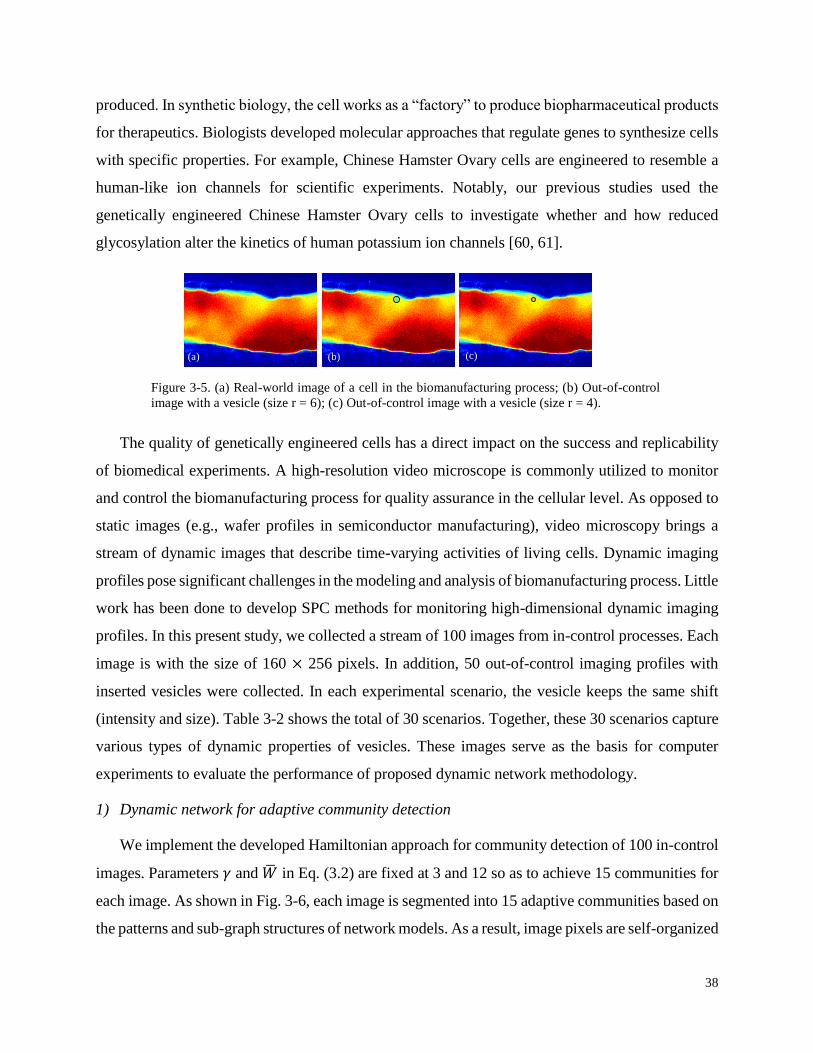
38
produced. In synthetic biology, the cell works as a “factory” to produce biopharmaceutical products
for therapeutics. Biologists developed molecular approaches that regulate genes to synthesize cells
with specific properties. For example, Chinese Hamster Ovary cells are engineered to resemble a
human-like ion channels for scientific experiments. Notably, our previous studies used the
genetically engineered Chinese Hamster Ovary cells to investigate whether and how reduced
glycosylation alter the kinetics of human potassium ion channels [60, 61].
The quality of genetically engineered cells has a direct impact on the success and replicability
of biomedical experiments. A high-resolution video microscope is commonly utilized to monitor
and control the biomanufacturing process for quality assurance in the cellular level. As opposed to
static images (e.g., wafer profiles in semiconductor manufacturing), video microscopy brings a
stream of dynamic images that describe time-varying activities of living cells. Dynamic imaging
profiles pose significant challenges in the modeling and analysis of biomanufacturing process. Little
work has been done to develop SPC methods for monitoring high-dimensional dynamic imaging
profiles. In this present study, we collected a stream of 100 images from in-control processes. Each
image is with the size of 160 × 256 pixels. In addition, 50 out-of-control imaging profiles with
inserted vesicles were collected. In each experimental scenario, the vesicle keeps the same shift
(intensity and size). Table 3-2 shows the total of 30 scenarios. Together, these 30 scenarios capture
various types of dynamic properties of vesicles. These images serve as the basis for computer
experiments to evaluate the performance of proposed dynamic network methodology.
1) Dynamic network for adaptive community detection
We implement the developed Hamiltonian approach for community detection of 100 in-control
images. Parameters 𝛾 and �̅� in Eq. (3.2) are fixed at 3 and 12 so as to achieve 15 communities for
each image. As shown in Fig. 3-6, each image is segmented into 15 adaptive communities based on
the patterns and sub-graph structures of network models. As a result, image pixels are self-organized
Figure 3-5. (a) Real-world image of a cell in the biomanufacturing process; (b) Out-of-control
image with a vesicle (size r = 6); (c) Out-of-control image with a vesicle (size r = 4).
(a) (b) (c)
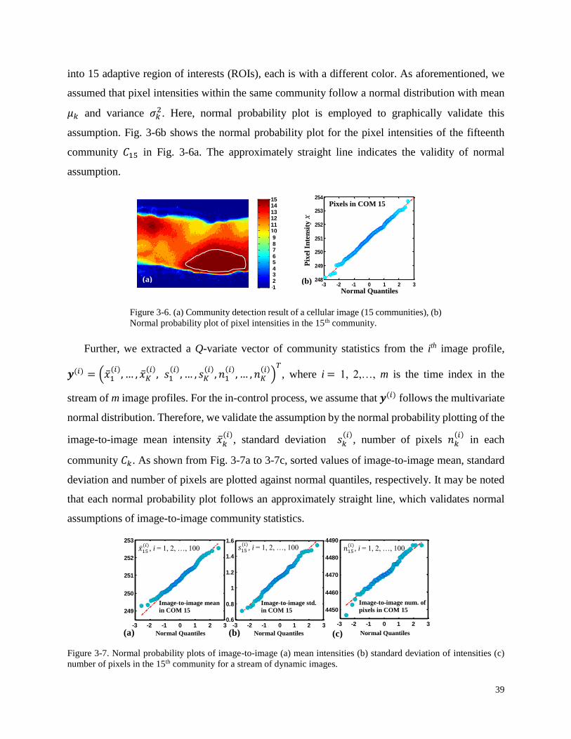
39
into 15 adaptive region of interests (ROIs), each is with a different color. As aforementioned, we
assumed that pixel intensities within the same community follow a normal distribution with mean
𝜇𝑘 and variance 𝜎𝑘2. Here, normal probability plot is employed to graphically validate this
assumption. Fig. 3-6b shows the normal probability plot for the pixel intensities of the fifteenth
community 𝐶15 in Fig. 3-6a. The approximately straight line indicates the validity of normal
assumption.
Further, we extracted a Q-variate vector of community statistics from the ith image profile,
𝒚(𝑖) = (�̅�1(𝑖)
, … , �̅�𝐾(𝑖), 𝑠1
(𝑖), … , 𝑠𝐾(𝑖), 𝑛1
(𝑖), … , 𝑛𝐾(𝑖))
𝑇
, where i = 1, 2,…, m is the time index in the
stream of m image profiles. For the in-control process, we assume that 𝒚(𝑖) follows the multivariate
normal distribution. Therefore, we validate the assumption by the normal probability plotting of the
image-to-image mean intensity �̅�𝑘(𝑖)
, standard deviation 𝑠𝑘(𝑖)
, number of pixels 𝑛𝑘(𝑖)
in each
community 𝐶𝑘. As shown from Fig. 3-7a to 3-7c, sorted values of image-to-image mean, standard
deviation and number of pixels are plotted against normal quantiles, respectively. It may be noted
that each normal probability plot follows an approximately straight line, which validates normal
assumptions of image-to-image community statistics.
Figure 3-7. Normal probability plots of image-to-image (a) mean intensities (b) standard deviation of intensities (c)
number of pixels in the 15th community for a stream of dynamic images.
Figure 3-6. (a) Community detection result of a cellular image (15 communities), (b)
Normal probability plot of pixel intensities in the 15th community.
-3 -2 -1 0 1 2 3248
249
250
251
252
253
254
Theoretical Quantiles
Qu
an
tile
s o
f p
ixel
inte
nsit
ies
123456789101112131415
123456789101112131415
Normal Quantiles
Pixels in COM 15
(a) (b)
Pix
el I
nte
nsi
ty 𝑥
-3 -2 -1 0 1 2 3
4450
4460
4470
4480
4490
Theoretical Quantiles
Qu
an
tile
s o
f p
ixel
inte
nsit
ies
-3 -2 -1 0 1 2 30.6
0.8
1
1.2
1.4
1.6
Theoretical Quantiles
Qu
an
tile
s o
f p
ixel
inte
nsit
ies
-3 -2 -1 0 1 2 3
249
250
251
252
253
Theoretical Quantiles
Qu
an
tile
s o
f p
ixel
inte
nsit
ies
Normal Quantiles Normal Quantiles Normal Quantiles
Image-to-image mean
in COM 15 Image-to-image std.
in COM 15 Image-to-image num. of
pixels in COM 15
�̅�15(𝑖)
, i = 1, 2, …, 100 𝑠15(𝑖)
, i = 1, 2, …, 100 𝑛15(𝑖)
, i = 1, 2, …, 100
(b) (c) (a)
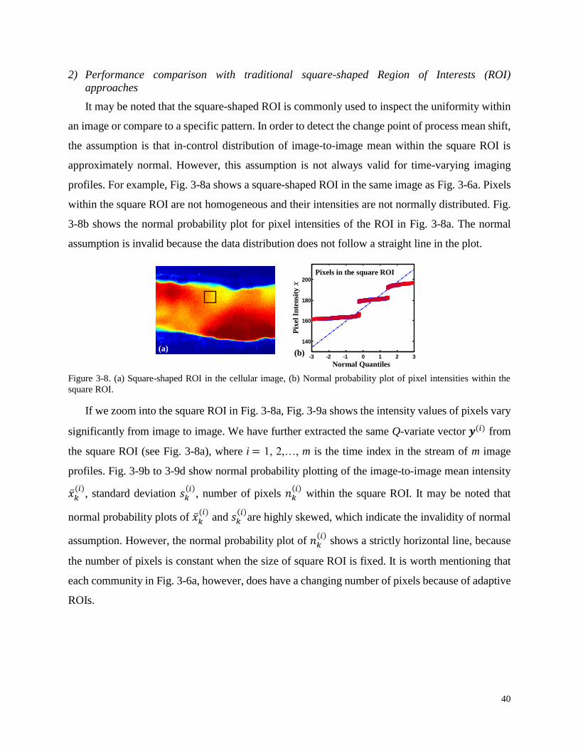
40
2) Performance comparison with traditional square-shaped Region of Interests (ROI)
approaches
It may be noted that the square-shaped ROI is commonly used to inspect the uniformity within
an image or compare to a specific pattern. In order to detect the change point of process mean shift,
the assumption is that in-control distribution of image-to-image mean within the square ROI is
approximately normal. However, this assumption is not always valid for time-varying imaging
profiles. For example, Fig. 3-8a shows a square-shaped ROI in the same image as Fig. 3-6a. Pixels
within the square ROI are not homogeneous and their intensities are not normally distributed. Fig.
3-8b shows the normal probability plot for pixel intensities of the ROI in Fig. 3-8a. The normal
assumption is invalid because the data distribution does not follow a straight line in the plot.
Figure 3-8. (a) Square-shaped ROI in the cellular image, (b) Normal probability plot of pixel intensities within the
square ROI.
If we zoom into the square ROI in Fig. 3-8a, Fig. 3-9a shows the intensity values of pixels vary
significantly from image to image. We have further extracted the same Q-variate vector 𝒚(𝑖) from
the square ROI (see Fig. 3-8a), where i = 1, 2,…, m is the time index in the stream of m image
profiles. Fig. 3-9b to 3-9d show normal probability plotting of the image-to-image mean intensity
�̅�𝑘(𝑖)
, standard deviation 𝑠𝑘(𝑖)
, number of pixels 𝑛𝑘(𝑖)
within the square ROI. It may be noted that
normal probability plots of �̅�𝑘(𝑖)
and 𝑠𝑘(𝑖)
are highly skewed, which indicate the invalidity of normal
assumption. However, the normal probability plot of 𝑛𝑘(𝑖)
shows a strictly horizontal line, because
the number of pixels is constant when the size of square ROI is fixed. It is worth mentioning that
each community in Fig. 3-6a, however, does have a changing number of pixels because of adaptive
ROIs.
-3 -2 -1 0 1 2 3
140
160
180
200
Theoretical Quantiles
Qu
an
tile
s o
f p
ixel
inte
nsit
ies
Normal Quantiles
Pix
el I
nte
nsi
ty 𝑥 Pixels in the square ROI
(b) (a)
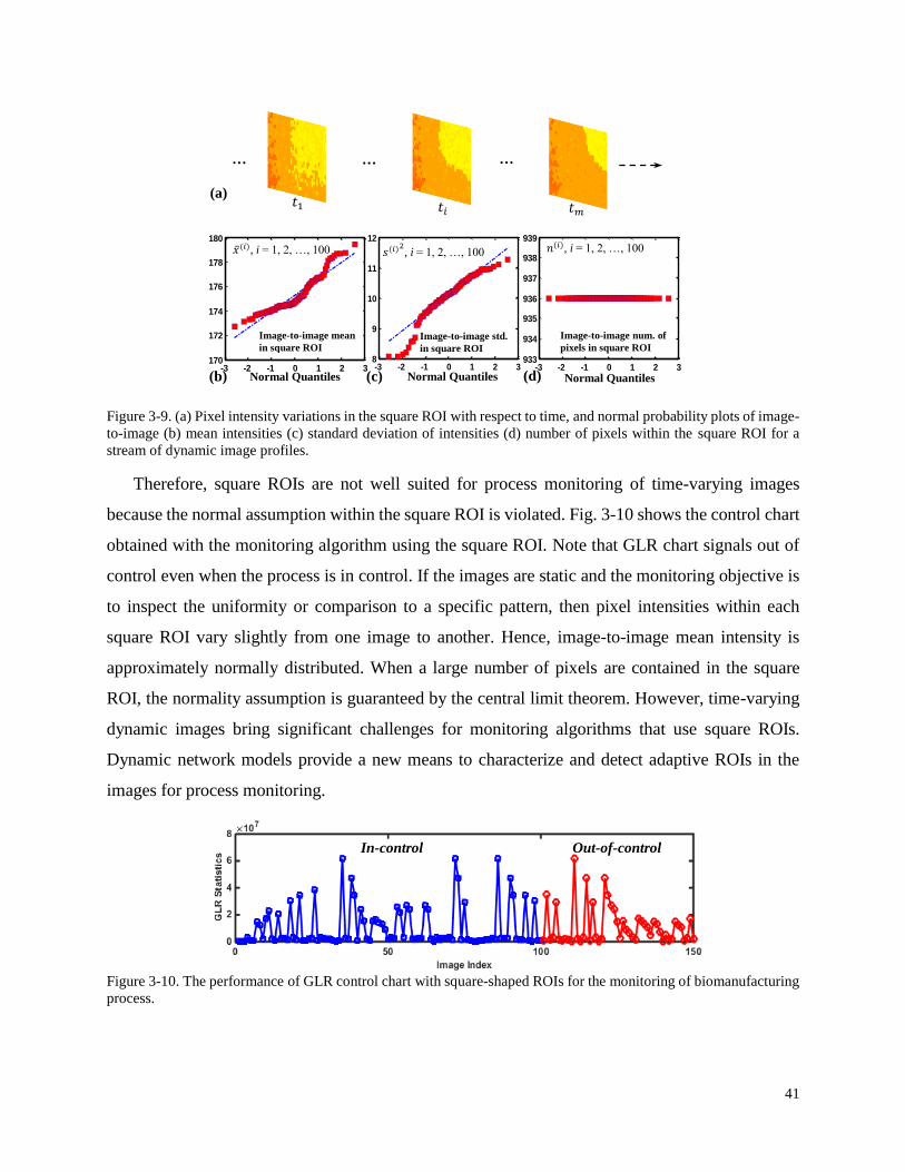
41
Figure 3-9. (a) Pixel intensity variations in the square ROI with respect to time, and normal probability plots of image-
to-image (b) mean intensities (c) standard deviation of intensities (d) number of pixels within the square ROI for a
stream of dynamic image profiles.
Therefore, square ROIs are not well suited for process monitoring of time-varying images
because the normal assumption within the square ROI is violated. Fig. 3-10 shows the control chart
obtained with the monitoring algorithm using the square ROI. Note that GLR chart signals out of
control even when the process is in control. If the images are static and the monitoring objective is
to inspect the uniformity or comparison to a specific pattern, then pixel intensities within each
square ROI vary slightly from one image to another. Hence, image-to-image mean intensity is
approximately normally distributed. When a large number of pixels are contained in the square
ROI, the normality assumption is guaranteed by the central limit theorem. However, time-varying
dynamic images bring significant challenges for monitoring algorithms that use square ROIs.
Dynamic network models provide a new means to characterize and detect adaptive ROIs in the
images for process monitoring.
Figure 3-10. The performance of GLR control chart with square-shaped ROIs for the monitoring of biomanufacturing
process.
-3 -2 -1 0 1 2 3933
934
935
936
937
938
939
Theoretical Quantiles
Qu
an
tile
s o
f p
ixel
inte
nsit
ies
-3 -2 -1 0 1 2 38
9
10
11
12
Theoretical Quantiles
Qu
an
tile
s o
f p
ixel
inte
nsit
ies
-3 -2 -1 0 1 2 3170
172
174
176
178
180
Theoretical Quantiles
Qu
an
tile
s o
f p
ixel
inte
nsit
ies
Normal Quantiles Normal Quantiles Normal Quantiles
Image-to-image mean
in square ROI Image-to-image std.
in square ROI Image-to-image num. of
pixels in square ROI
�̅�(𝑖), i = 1, 2, …, 100 𝑠(𝑖)2, i = 1, 2, …, 100 𝑛(𝑖), i = 1, 2, …, 100
(a) 𝑡1 𝑡𝑖 𝑡𝑚
… … …
(b) (c) (d)
In-control Out-of-control

42
3) Performance comparison between NGLR and 𝑇2charts
Furthermore, we conducted computer experiments to compare the performance of network GLR
and Hotelling 𝑇2charts for biomanufacturing process monitoring. It is worth mentioning that either
network GLR or 𝑇2 chart is calculated from the Q-variate vector of network community statistics.
𝑇2 statistics are calculated based on features extracted from network modeling and characterization
of image data. Note that the first 100 images are in-control profiles of cell dynamics. A vesicle with
transgenes is inserted into the cell after the 100th image (𝜏 = 100). We varied the intensity shift (∆𝑥)
and the radius (r) of inserted vesicles to evaluate the performances of the developed network GLR
algorithms. In total, there are 30 scenarios including 3 levels of radius and 10 levels of intensity
shifts. Average run length is used as a metric to evaluate the performance of monitoring schemes.
ARL is the average period after which the process-monitoring scheme first signals the out-of-
control image profile. In this study, we focused on Phase II out-of-control ARLs (i.e., ARL1).
Notably, ARL1s are calculated by randomly replicating each scenario for 100 times.
For the 𝑖𝑡ℎ image profile, the Hotelling 𝑇2 statistic is computed using the Q-variate vector of
network community statistics 𝒚(𝑖) as:
𝑇2(𝑖) = (𝒚(𝑖) − �̅�)𝑇 𝑺−1(𝒚(𝑖) − �̅�) (3.15)
In order to address the singular issue of the covariance matrix 𝑺, we computed the 𝑇2 statistic in
Eq. (3.15) using the set of principal components as in our previous study [53]:
𝑇2(𝑖) = (𝒚(𝑖) − �̅�)𝑇 𝑺−1(𝒚(𝑖) − �̅�) = ∑
𝐙(𝑖, 𝑟)2
𝜆𝑟2
𝑄
𝑟=1
(3.16)
In addition, we considered the first 𝑞 principal components (𝑞 < 𝑄) to obtain the Hotelling 𝑇2
statistic in the reduced dimension 𝑞 as:
𝑇2(𝑖) = ∑𝐙(𝑖, 𝑟)2
𝜆𝑟2
𝑞
𝑟=1
(3.17)

43
This reduced-dimension 𝑇2 statistic will be further used in the next section to benchmark the
performance of network GLR chart in the reduced dimension. Notably, the upper control limit
(UCL) of Hotelling 𝑇2control chart is estimated as:
𝑈𝐶𝐿𝑇2 = 𝑞(𝑀 + 1)(𝑀 − 1)
𝑀2 − 𝑀𝑞𝐹𝛼,𝑞,𝑀−𝑞 (3.18)
where q is the number of features (i.e., the dimensionality of 𝒚(𝑖)), M is the number of imaging
profiles, 𝐹𝛼,𝑞,𝑀−𝑞 is the upper 100𝛼% of critical point of F distribution with 𝑞 and 𝑀 − 𝑞 degree
of freedoms. The significance level 𝛼 is set as 0.05.
Table 3-2 shows the results of performance comparison between NGLR and Hotelling 𝑇2 charts
for 30 scenarios of varying size (r) and intensity shift (∆𝑥) of the vesicle. Experiments were
replicated 100 times for each scenario. When the intensity shift is large, ARL1s of both charts reach
1.00. In other words, one sample is adequate on average for the monitoring scheme to first signal
the vesicle. For instance, both charts have ARL1 values of 1.00 when |∆𝑥| = 10, which means the
vesicle is immediately detected when it emerges. When the intensity shift is decreased to |∆𝑥| = 7
and 8, the ARL1 begin to increase. Notably, ARL1 is bigger for the scenarios with smaller radius of
vesicles. For example, both charts yield ARL1s of 1.00 when ∆𝑥 = 8 and r = 8, while the ARL1 of
NGLR chart is increased to 1.63 and the ARL1 of 𝑇2 chart reaches 4.88 when ∆𝑥 = 8 and r = 4.
When the intensity shift is very small (i.e., |∆𝑥| = 5 and 6), NGLR charts signal the out-of-control
faster than 𝑇2 charts. For example, NGLR chart yields the ARL1 of 3.38 for ∆𝑥 = 5, 𝑟 = 4 and
3.71 for ∆𝑥 = −5, 𝑟 = 4, while 𝑇2 chart are 16.69 (for ∆𝑥 = 5) and 14.96 (for ∆𝑥 = −5).

44
Table 3-2 also shows the distribution of ∆𝜏 for 100 replications, which is the time delay between
signaled change point (�̂�) and actual change point (𝜏). Smaller delay ∆𝜏 indicates better
performances in the change-point detection. When the intensity shift is large (i.e.,|∆𝑥| = 10), both
NGLR and 𝑇2 charts yield the time delay ∆𝜏= 0 for 100 replications and only slight deviation to
∆𝜏∈(0, 3] when ∆𝑥 = 10 and 𝑟 = 4. In other words, both charts immediately signal the out-of-
control sample. When the intensity shift is decreased to |∆𝑥| = 7 and 8, most of replications reside
in the intervals ∆𝜏∈[0, 3] and (3, 10]. Nonetheless, NGLR charts have more replications with shorter
time delays ∆𝜏 and thereby perform better than 𝑇2 chart. The 𝑇2 chart also has ∆𝜏> 10 for a fraction
of replications (e.g., 27 replications for ∆𝑥 = 7, 𝑟 = 4). When the intensity shift is very small (i.e.,
|∆𝑥| = 5 or 6), 100 replications spread over the intervals ∆𝜏∈[0, 3], (3, 10] and [10, +∞]. Table 3-2
shows that NGLR charts have more replications with shorter time delays ∆𝜏, thereby performing
better than 𝑇2 chart. Notably, time delay ∆𝜏 is bigger for the scenarios with smaller radius of
vesicles.
Table 3-2. Performance Comparison Between Network GLR and Hotelling 𝑇2 Charts
∆ r ARL1
Distribution of ∆𝜏 = �̂� − 𝜏
∆𝜏 = 0 0 < ∆𝜏 ≤3 3 < ∆𝜏 ≤10 ∆𝜏>10
NGLR 𝑇2 NGLR 𝑇2 NGLR 𝑇2 NGLR 𝑇2 NGLR 𝑇2
-10
4 1.00 1.00 100 100 0 0 0 0 0 0
6 1.00 1.00 100 100 0 0 0 0 0 0
8 1.00 1.00 100 100 0 0 0 0 0 0
-8
4 1.24 1.90 78 51 22 39 0 10 0 0
6 1.01 1.05 99 95 1 5 0 0 0 0
8 1.00 1.00 100 100 0 0 0 0 0 0
-7
4 2.18 4.44 37 22 49 30 14 40 0 8
6 1.10 1.60 90 61 10 34 0 5 0 0
8 1.00 1.02 100 98 0 2 0 0 0 0
-6
4 2.56 13.30 23 7 56 9 21 32 0 51
6 1.41 3.44 61 28 39 31 0 41 0 0
8 1.06 1.23 94 82 6 18 0 0 0 0
-5
4 3.71 14.96 18 7 39 10 40 29 3 46
6 1.98 7.37 34 14 60 22 6 40 0 24
8 1.30 2.36 71 42 29 39 0 17 0 2
5
4 3.38 16.69 24 4 41 9 33 25 2 55
6 1.82 6.00 43 23 54 19 3 42 0 16
8 1.25 2.04 76 48 24 37 0 15 0 0
6
4 3.01 11.11 21 11 46 14 33 33 0 41
6 1.47 3.24 62 33 38 36 0 30 0 1
8 1.03 1.15 97 86 3 14 0 0 0 0
7
4 2.18 7.23 35 9 53 31 12 33 0 27
6 1.13 1.51 87 67 13 29 0 4 0 0
8 1.00 1.00 100 100 0 0 0 0 0 0
8
4 1.63 4.88 53 19 44 34 3 36 0 11
6 1.03 1.17 97 85 3 15 0 0 0 0
8 1.00 1.00 100 100 0 0 0 0 0 0
10
4 1.05 1.11 96 90 4 10 0 0 0 0
6 1.00 1.00 100 100 0 0 0 0 0 0
8 1.00 1.00 100 100 0 0 0 0 0 0

45
It should be noted that both NGLR and 𝑇2 chart are established based on the Q-variate vector
of network community statistics. Table 3-2 shows that both charts perform well in the change-point
detection, but NGLR chart signals the out-of-control quicker than 𝑇2 chart. This is because NGLR
chart not only considers the present imaging profile, but also tracks historical imaging profiles
within a sliding window to identify the maximal change in the likelihood ratio (also see Eq. (3.11)
and Eq. (3.15)). However, computational complexity of NGLR is slightly higher than that of 𝑇2
chart due to the computation of likelihood ratio in the sliding window. In practice, the tradeoff
between performance and computational complexity needs to be considered in the selection of
control chart for the purpose of process monitoring.
4) Dynamic network GLR chart in the reduced dimension
Furthermore, we conducted experiments to investigate the performance of dynamic network
GLR charts in the reduced dimension. Notably, Table 3-2 is obtained with the complete set of
community statistics (45 features = 15 communities × 3 statistics in each community). The next
step is to evaluate the performance of NGLR and 𝑇2 charts in the reduced dimension. Monitoring
schemes with a low-dimensional set of features tend to be more efficient because of the simplified
model form. Therefore, we reduced the dimensionality of Q-variate vector of network community
statistics by keeping the first 𝑞 principal components with relatively large eigenvalues that explain
the majority of data variance. The Pareto chart in Fig. 3-11 shows the percentage of variance
explained by principal components (PC) that are sorted with respect to the descending eigenvalues.
The first PC with the largest eigenvalue explains 20% of total variance. It should be noted that Fig.
3-11 does not have a few predominant PCs (e.g., < 5) that explain more than 90% of total variance.
A total of 30 principal components are necessary to achieve the performance to explain 95% of total
data variance.
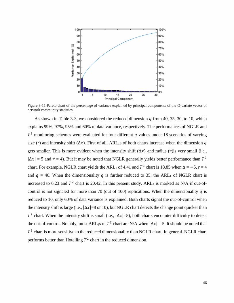
46
Figure 3-11 Pareto chart of the percentage of variance explained by principal components of the Q-variate vector of
network community statistics.
As shown in Table 3-3, we considered the reduced dimension 𝑞 from 40, 35, 30, to 10, which
explains 99%, 97%, 95% and 60% of data variance, respectively. The performances of NGLR and
𝑇2 monitoring schemes were evaluated for four different 𝑞 values under 18 scenarios of varying
size (r) and intensity shift (∆𝑥). First of all, ARL1s of both charts increase when the dimension 𝑞
gets smaller. This is more evident when the intensity shift (∆𝑥) and radius (𝑟)is very small (i.e.,
|∆𝑥| = 5 and 𝑟 = 4). But it may be noted that NGLR generally yields better performance than 𝑇2
chart. For example, NGLR chart yields the ARL1 of 4.41 and 𝑇2 chart is 18.85 when ∆ = −5, r = 4
and 𝑞 = 40. When the dimensionality 𝑞 is further reduced to 35, the ARL1 of NGLR chart is
increased to 6.23 and 𝑇2 chart is 20.42. In this present study, ARL1 is marked as N/A if out-of-
control is not signaled for more than 70 (out of 100) replications. When the dimensionality 𝑞 is
reduced to 10, only 60% of data variance is explained. Both charts signal the out-of-control when
the intensity shift is large (i.e., |∆𝑥|=8 or 10), but NGLR chart detects the change point quicker than
𝑇2 chart. When the intensity shift is small (i.e., |∆𝑥|=5), both charts encounter difficulty to detect
the out-of-control. Notably, most ARL1s of 𝑇2 chart are N/A when |∆𝑥| = 5. It should be noted that
𝑇2 chart is more sensitive to the reduced dimensionality than NGLR chart. In general. NGLR chart
performs better than Hotelling 𝑇2 chart in the reduced dimension.
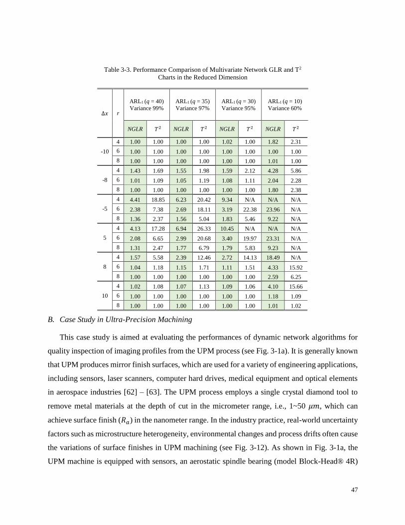
47
Table 3-3. Performance Comparison of Multivariate Network GLR and T2
Charts in the Reduced Dimension
∆𝑥 r
ARL1 (q = 40)
Variance 99% ARL1 (q = 35)
Variance 97% ARL1 (q = 30)
Variance 95% ARL1 (q = 10)
Variance 60%
NGLR 𝑇2 NGLR 𝑇2 NGLR 𝑇2 NGLR 𝑇2
-10
4 1.00 1.00 1.00 1.00 1.02 1.00 1.82 2.31
6 1.00 1.00 1.00 1.00 1.00 1.00 1.00 1.00
8 1.00 1.00 1.00 1.00 1.00 1.00 1.01 1.00
-8
4 1.43 1.69 1.55 1.98 1.59 2.12 4.28 5.86
6 1.01 1.09 1.05 1.19 1.08 1.11 2.04 2.28
8 1.00 1.00 1.00 1.00 1.00 1.00 1.80 2.38
-5
4 4.41 18.85 6.23 20.42 9.34 N/A N/A N/A
6 2.38 7.38 2.69 18.11 3.19 22.38 23.96 N/A
8 1.36 2.37 1.56 5.04 1.83 5.46 9.22 N/A
5
4 4.13 17.28 6.94 26.33 10.45 N/A N/A N/A
6 2.08 6.65 2.99 20.68 3.40 19.97 23.31 N/A
8 1.31 2.47 1.77 6.79 1.79 5.83 9.23 N/A
8
4 1.57 5.58 2.39 12.46 2.72 14.13 18.49 N/A
6 1.04 1.18 1.15 1.71 1.11 1.51 4.33 15.92
8 1.00 1.00 1.00 1.00 1.00 1.00 2.59 6.25
10
4 1.02 1.08 1.07 1.13 1.09 1.06 4.10 15.66
6 1.00 1.00 1.00 1.00 1.00 1.00 1.18 1.09
8 1.00 1.00 1.00 1.00 1.00 1.00 1.01 1.02
B. Case Study in Ultra-Precision Machining
This case study is aimed at evaluating the performances of dynamic network algorithms for
quality inspection of imaging profiles from the UPM process (see Fig. 3-1a). It is generally known
that UPM produces mirror finish surfaces, which are used for a variety of engineering applications,
including sensors, laser scanners, computer hard drives, medical equipment and optical elements
in aerospace industries [62] – [63]. The UPM process employs a single crystal diamond tool to
remove metal materials at the depth of cut in the micrometer range, i.e., 1~50 𝜇𝑚, which can
achieve surface finish (𝑅𝑎) in the nanometer range. In the industry practice, real-world uncertainty
factors such as microstructure heterogeneity, environmental changes and process drifts often cause
the variations of surface finishes in UPM machining (see Fig. 3-12). As shown in Fig. 3-1a, the
UPM machine is equipped with sensors, an aerostatic spindle bearing (model Block-Head® 4R)
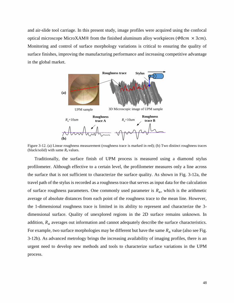
48
and air-slide tool carriage. In this present study, image profiles were acquired using the confocal
optical microscope MicroXAM® from the finished aluminum alloy workpieces (𝛷8𝑐𝑚 × 3𝑐𝑚).
Monitoring and control of surface morphology variations is critical to ensuring the quality of
surface finishes, improving the manufacturing performance and increasing competitive advantage
in the global market.
Figure 3-12. (a) Linear roughness measurement (roughness trace is marked in red); (b) Two distinct roughness traces
(black/solid) with same Ra values.
Traditionally, the surface finish of UPM process is measured using a diamond stylus
profilometer. Although effective to a certain level, the profilometer measures only a line across
the surface that is not sufficient to characterize the surface quality. As shown in Fig. 3-12a, the
travel path of the stylus is recorded as a roughness trace that serves as input data for the calculation
of surface roughness parameters. One commonly used parameter is 𝑅𝑎, which is the arithmetic
average of absolute distances from each point of the roughness trace to the mean line. However,
the 1-dimensional roughness trace is limited in its ability to represent and characterize the 3-
dimensional surface. Quality of unexplored regions in the 2D surface remains unknown. In
addition, 𝑅𝑎 averages out information and cannot adequately describe the surface characteristics.
For example, two surface morphologies may be different but have the same 𝑅𝑎 value (also see Fig.
3-12b). As advanced metrology brings the increasing availability of imaging profiles, there is an
urgent need to develop new methods and tools to characterize surface variations in the UPM
process.
Roughness
trace B Ra=10um Ra=10um Roughness
trace A
Stylus Roughness trace
(a)
(b)
UPM sample 3D Microscopic image of UPM sample
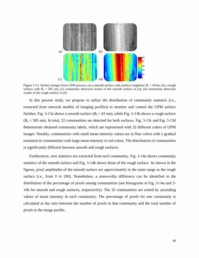
49
Figure 3-13. Surface images from UPM process, (a) a smooth surface with surface roughness Ra = 43nm; (b) a rough
surface with Ra = 585 nm; (c) community detection results of the smooth surface in (a); (d) community detection
results of the rough surface in (b).
In this present study, we propose to utilize the distribution of community statistics (i.e.,
extracted from network models of imaging profiles) to monitor and control the UPM surface
finishes. Fig. 3-13a shows a smooth surface (Ra = 43 nm), while Fig. 3-13b shows a rough surface
(Ra = 585 nm). In total, 32 communities are detected for both surfaces. Fig. 3-13c and Fig. 3-13d
demonstrate obtained community labels, which are represented with 32 different colors of UPM
images. Notably, communities with small mean intensity values are in blue colors with a gradual
transition to communities with large mean intensity in red colors. The distribution of communities
is significantly different between smooth and rough surfaces.
Furthermore, new statistics are extracted from each community. Fig. 3-14a shows community
statistics of the smooth surface and Fig. 3-14b shows those of the rough surface. As shown in the
figures, pixel amplitudes of the smooth surface are approximately in the same range as the rough
surface (i.e., from 0 to 200). Nonetheless, a noteworthy difference can be identified in the
distribution of the percentage of pixels among communities (see histograms in Fig. 3-14a and 3-
14b for smooth and rough surfaces, respectively). The 32 communities are sorted by ascending
values of mean intensity in each community. The percentage of pixels for one community is
calculated as the ratio between the number of pixels in that community and the total number of
pixels in the image profile.
(a) (b)
(c) (d)
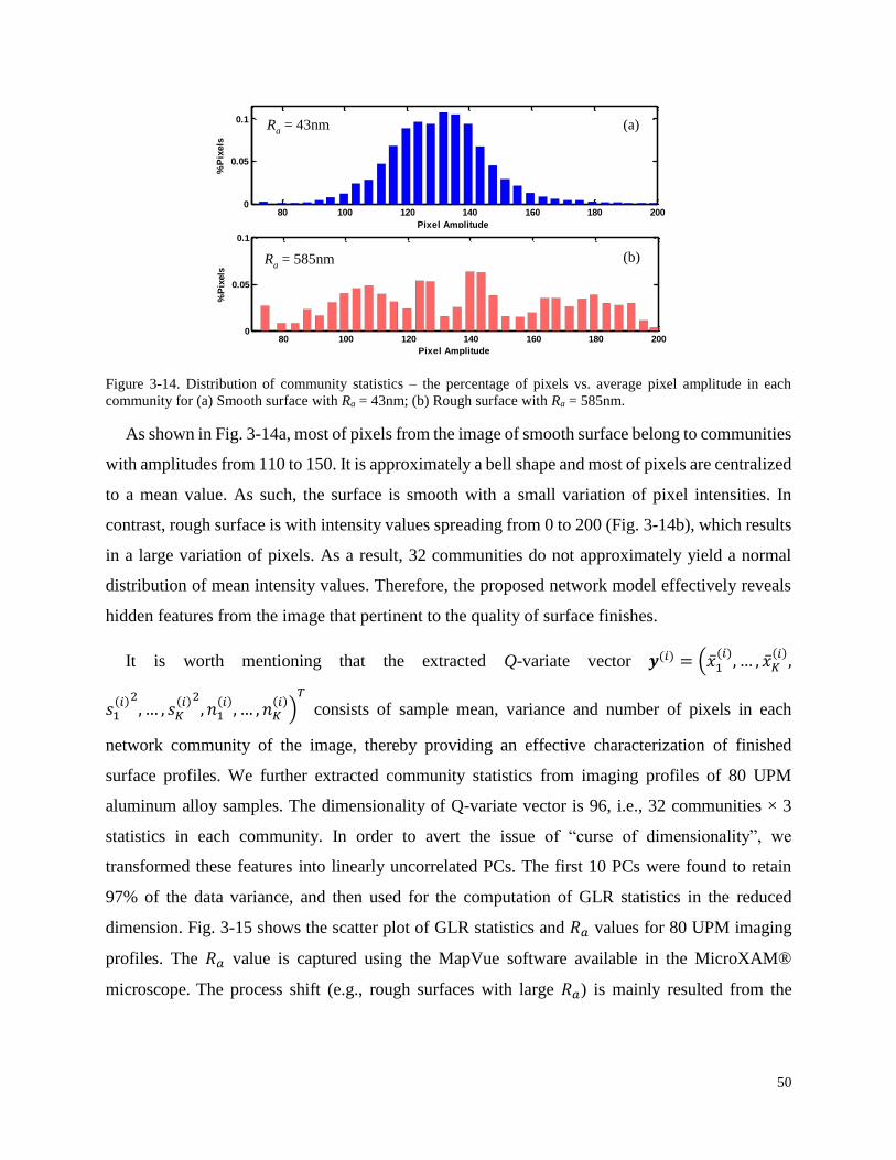
50
Figure 3-14. Distribution of community statistics – the percentage of pixels vs. average pixel amplitude in each
community for (a) Smooth surface with Ra = 43nm; (b) Rough surface with Ra = 585nm.
As shown in Fig. 3-14a, most of pixels from the image of smooth surface belong to communities
with amplitudes from 110 to 150. It is approximately a bell shape and most of pixels are centralized
to a mean value. As such, the surface is smooth with a small variation of pixel intensities. In
contrast, rough surface is with intensity values spreading from 0 to 200 (Fig. 3-14b), which results
in a large variation of pixels. As a result, 32 communities do not approximately yield a normal
distribution of mean intensity values. Therefore, the proposed network model effectively reveals
hidden features from the image that pertinent to the quality of surface finishes.
It is worth mentioning that the extracted Q-variate vector 𝒚(𝑖) = (�̅�1(𝑖)
, … , �̅�𝐾(𝑖),
𝑠1(𝑖)2, … , 𝑠𝐾
(𝑖)2, 𝑛1(𝑖), … , 𝑛𝐾
(𝑖))𝑇
consists of sample mean, variance and number of pixels in each
network community of the image, thereby providing an effective characterization of finished
surface profiles. We further extracted community statistics from imaging profiles of 80 UPM
aluminum alloy samples. The dimensionality of Q-variate vector is 96, i.e., 32 communities × 3
statistics in each community. In order to avert the issue of “curse of dimensionality”, we
transformed these features into linearly uncorrelated PCs. The first 10 PCs were found to retain
97% of the data variance, and then used for the computation of GLR statistics in the reduced
dimension. Fig. 3-15 shows the scatter plot of GLR statistics and 𝑅𝑎 values for 80 UPM imaging
profiles. The 𝑅𝑎 value is captured using the MapVue software available in the MicroXAM®
microscope. The process shift (e.g., rough surfaces with large 𝑅𝑎) is mainly resulted from the
80 100 120 140 160 180 2000
0.05
0.1
Pixel Amplitude%
Pix
els
80 100 120 140 160 180 2000
0.05
0.1
Pixel Amplitude
%P
ixels
Ra = 43nm
Ra = 585nm
(a)
(b)
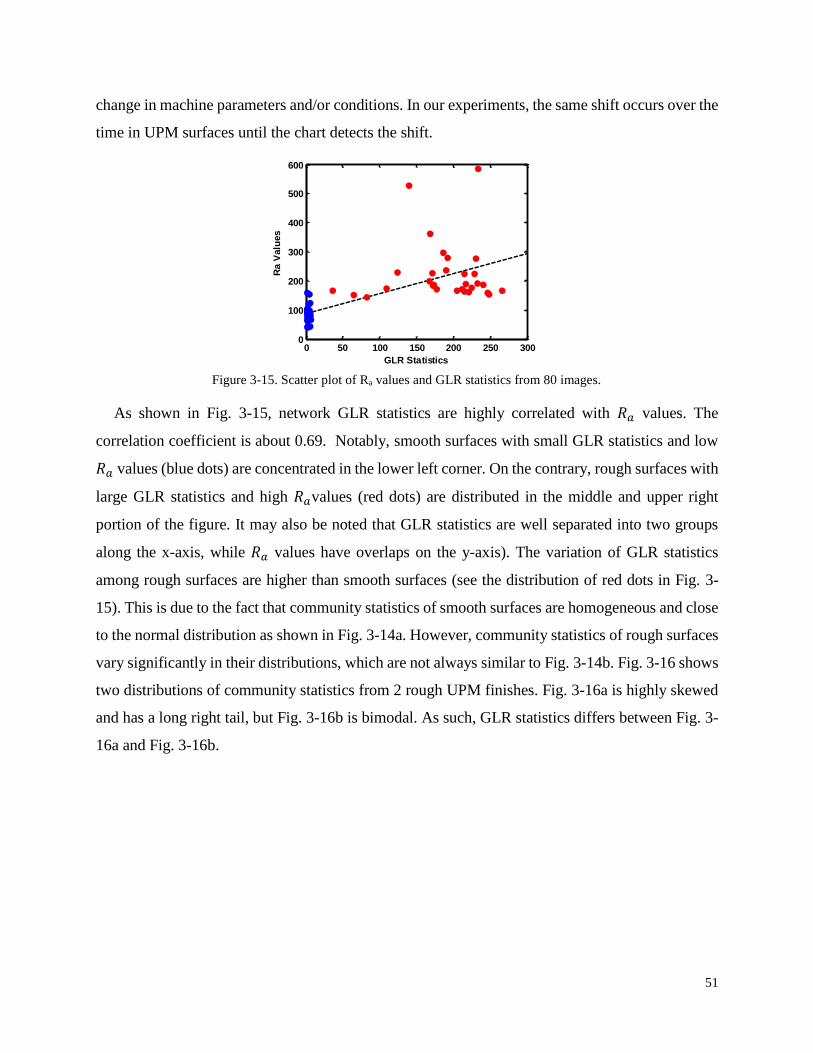
51
change in machine parameters and/or conditions. In our experiments, the same shift occurs over the
time in UPM surfaces until the chart detects the shift.
As shown in Fig. 3-15, network GLR statistics are highly correlated with 𝑅𝑎 values. The
correlation coefficient is about 0.69. Notably, smooth surfaces with small GLR statistics and low
𝑅𝑎 values (blue dots) are concentrated in the lower left corner. On the contrary, rough surfaces with
large GLR statistics and high 𝑅𝑎values (red dots) are distributed in the middle and upper right
portion of the figure. It may also be noted that GLR statistics are well separated into two groups
along the x-axis, while 𝑅𝑎 values have overlaps on the y-axis). The variation of GLR statistics
among rough surfaces are higher than smooth surfaces (see the distribution of red dots in Fig. 3-
15). This is due to the fact that community statistics of smooth surfaces are homogeneous and close
to the normal distribution as shown in Fig. 3-14a. However, community statistics of rough surfaces
vary significantly in their distributions, which are not always similar to Fig. 3-14b. Fig. 3-16 shows
two distributions of community statistics from 2 rough UPM finishes. Fig. 3-16a is highly skewed
and has a long right tail, but Fig. 3-16b is bimodal. As such, GLR statistics differs between Fig. 3-
16a and Fig. 3-16b.
0 50 100 150 200 250 3000
100
200
300
400
500
600
GLR Statistics
Ra V
alu
es
Figure 3-15. Scatter plot of Ra values and GLR statistics from 80 images.
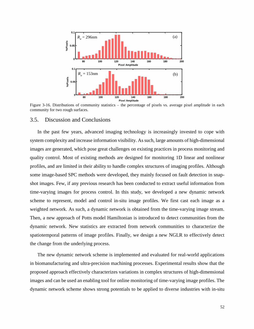
52
Figure 3-16. Distributions of community statistics – the percentage of pixels vs. average pixel amplitude in each
community for two rough surfaces.
3.5. Discussion and Conclusions
In the past few years, advanced imaging technology is increasingly invested to cope with
system complexity and increase information visibility. As such, large amounts of high-dimensional
images are generated, which pose great challenges on existing practices in process monitoring and
quality control. Most of existing methods are designed for monitoring 1D linear and nonlinear
profiles, and are limited in their ability to handle complex structures of imaging profiles. Although
some image-based SPC methods were developed, they mainly focused on fault detection in snap-
shot images. Few, if any previous research has been conducted to extract useful information from
time-varying images for process control. In this study, we developed a new dynamic network
scheme to represent, model and control in-situ image profiles. We first cast each image as a
weighted network. As such, a dynamic network is obtained from the time-varying image stream.
Then, a new approach of Potts model Hamiltonian is introduced to detect communities from the
dynamic network. New statistics are extracted from network communities to characterize the
spatiotemporal patterns of image profiles. Finally, we design a new NGLR to effectively detect
the change from the underlying process.
The new dynamic network scheme is implemented and evaluated for real-world applications
in biomanufacturing and ultra-precision machining processes. Experimental results show that the
proposed approach effectively characterizes variations in complex structures of high-dimensional
images and can be used an enabling tool for online monitoring of time-varying image profiles. The
dynamic network scheme shows strong potentials to be applied to diverse industries with in-situ
80 100 120 140 160 180 2000
0.05
0.1
Pixel Amplitude%
Pix
els
80 100 120 140 160 180 2000
0.05
0.1
Pixel Amplitude
%P
ixels
Ra = 296nm
Ra = 153nm
(a)
(b)

53
imaging data. While existing statistical methods mainly focus on the modeling and analysis of 2D
images, dynamic network has advantageous features to effectively represent high-dimensional
imaging profiles (i.e., > 2D images), Network nodes are flexible to represent pixels in 3D, 4D and
multi-dimensional images. Network edges effectively characterize spatiotemporal patterns in the
stream of images. In the future, we will further investigate and develop network methods and tools
for quality control of complex spatial patterns in 3D/4D image streams.
54
Chapter 4: Parallel Computing and Network Analytics for Fast
Industrial Internet-of-Things (IIoT) Machine Information
Processing and Condition Monitoring
Abstract
Rapid advancement in sensing, communication, and mobile technologies brings a new wave of
Industrial Internet of Things (IIoT) technology. IIoT integrates a large number of sensors for smart
and connected monitoring of machine conditions. Sensor observations contain rich information on
operational signatures of machines, thereby providing a great opportunity for machine condition
monitoring and control in the context of large-scale IIoT. However, realizing the full potential of
IIoT depends to a great extent on the development of new methodologies using big data analytics.
Existing approaches are limited in their ability to effectively extract pertinent knowledge about
manufacturing operations from the large volume of IIoT data of networked machines. This paper
presents new parallel algorithms for large-scale IIoT machine information processing, network
modeling, condition monitoring, and fault diagnosis. First, we introduce a dynamic time warping
algorithm to characterize and quantify the dissimilarity of machine signatures (e.g., power profiles
during operations). Second, we develop a stochastic network embedding algorithm to construct a
large-scale network of IIoT machines, in which the dissimilarity between machine signatures is
preserved in the network node-to-node distance. When the machine condition varies, the location
of the corresponding network node changes accordingly. As such, node locations will provide
diagnostic information about machine conditions. However, the network embedding algorithm is
computationally expensive in the presence of large amounts of IIoT enabled machines. Therefore,
we further develop a parallel algorithm that harnesses the power of multiple processors for efficient
network modeling of large-scale IIoT enabled machines. Experimental results show that the new
parallel-computing algorithm efficiently and effectively characterizes the variations of machine
signatures for network modeling and monitoring. This new approach shows strong potentials for
optimal machine scheduling and maintenance in the context of large-scale IIoT.
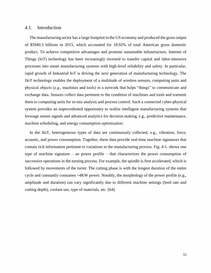
55
4.1. Introduction
The manufacturing sector has a large footprint in the US economy and produced the gross output
of $5940.3 billions in 2015, which accounted for 18.92% of total American gross domestic
product. To achieve competitive advantages and promote sustainable infrastructure, Internet of
Things (IoT) technology has been increasingly invested to transfer capital and labor-intensive
processes into smart manufacturing systems with high-level reliability and safety. In particular,
rapid growth of Industrial IoT is driving the next generation of manufacturing technology. The
IIoT technology enables the deployment of a multitude of wireless sensors, computing units and
physical objects (e.g., machines and tools) in a network that helps “things” to communicate and
exchange data. Sensors collect data pertinent to the condition of machines and tools and transmit
them to computing units for in-situ analysis and process control. Such a connected cyber-physical
system provides an unprecedented opportunity to realize intelligent manufacturing systems that
leverage sensor signals and advanced analytics for decision making, e.g., predictive maintenance,
machine scheduling, and energy consumption optimization.
In the IIoT, heterogeneous types of data are continuously collected, e.g., vibration, force,
acoustic, and power consumption. Together, these data provide real-time machine signatures that
contain rich information pertinent to variations in the manufacturing process. Fig. 4-1. shows one
type of machine signature – an power profile – that characterizes the power consumption of
successive operations in the turning process. For example, the spindle is first accelerated, which is
followed by movements of the turret. The cutting phase is with the longest duration of the entire
cycle and constantly consumes ~4KW power. Notably, the morphology of the power profile (e.g.,
amplitude and duration) can vary significantly due to different machine settings (feed rate and
cutting depth), coolant use, type of materials, etc. [64].
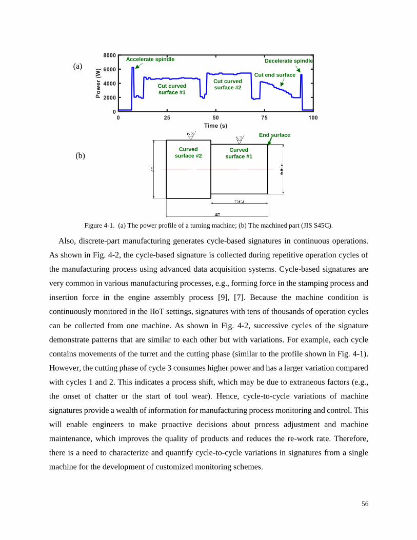
56
Figure 4-1. (a) The power profile of a turning machine; (b) The machined part (JIS S45C).
Also, discrete-part manufacturing generates cycle-based signatures in continuous operations.
As shown in Fig. 4-2, the cycle-based signature is collected during repetitive operation cycles of
the manufacturing process using advanced data acquisition systems. Cycle-based signatures are
very common in various manufacturing processes, e.g., forming force in the stamping process and
insertion force in the engine assembly process [9], [7]. Because the machine condition is
continuously monitored in the IIoT settings, signatures with tens of thousands of operation cycles
can be collected from one machine. As shown in Fig. 4-2, successive cycles of the signature
demonstrate patterns that are similar to each other but with variations. For example, each cycle
contains movements of the turret and the cutting phase (similar to the profile shown in Fig. 4-1).
However, the cutting phase of cycle 3 consumes higher power and has a larger variation compared
with cycles 1 and 2. This indicates a process shift, which may be due to extraneous factors (e.g.,
the onset of chatter or the start of tool wear). Hence, cycle-to-cycle variations of machine
signatures provide a wealth of information for manufacturing process monitoring and control. This
will enable engineers to make proactive decisions about process adjustment and machine
maintenance, which improves the quality of products and reduces the re-work rate. Therefore,
there is a need to characterize and quantify cycle-to-cycle variations in signatures from a single
machine for the development of customized monitoring schemes.
Accelerate spindle
Cut end surface
Decelerate spindle
Cut curved
surface #1
Cut curved surface #2
Curved
surface #2 Curved
surface #1
End surface
(a)
(b)
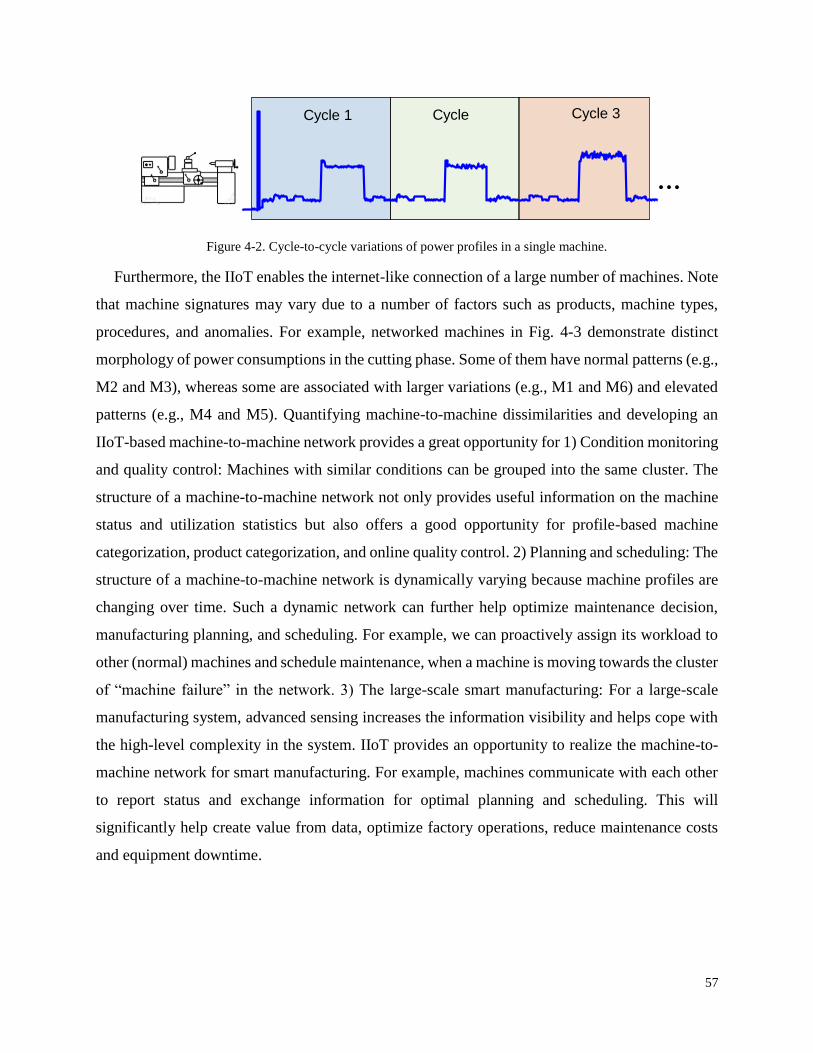
57
Figure 4-2. Cycle-to-cycle variations of power profiles in a single machine.
Furthermore, the IIoT enables the internet-like connection of a large number of machines. Note
that machine signatures may vary due to a number of factors such as products, machine types,
procedures, and anomalies. For example, networked machines in Fig. 4-3 demonstrate distinct
morphology of power consumptions in the cutting phase. Some of them have normal patterns (e.g.,
M2 and M3), whereas some are associated with larger variations (e.g., M1 and M6) and elevated
patterns (e.g., M4 and M5). Quantifying machine-to-machine dissimilarities and developing an
IIoT-based machine-to-machine network provides a great opportunity for 1) Condition monitoring
and quality control: Machines with similar conditions can be grouped into the same cluster. The
structure of a machine-to-machine network not only provides useful information on the machine
status and utilization statistics but also offers a good opportunity for profile-based machine
categorization, product categorization, and online quality control. 2) Planning and scheduling: The
structure of a machine-to-machine network is dynamically varying because machine profiles are
changing over time. Such a dynamic network can further help optimize maintenance decision,
manufacturing planning, and scheduling. For example, we can proactively assign its workload to
other (normal) machines and schedule maintenance, when a machine is moving towards the cluster
of “machine failure” in the network. 3) The large-scale smart manufacturing: For a large-scale
manufacturing system, advanced sensing increases the information visibility and helps cope with
the high-level complexity in the system. IIoT provides an opportunity to realize the machine-to-
machine network for smart manufacturing. For example, machines communicate with each other
to report status and exchange information for optimal planning and scheduling. This will
significantly help create value from data, optimize factory operations, reduce maintenance costs
and equipment downtime.
…
Cycle 1 Cycle
2
Cycle 3
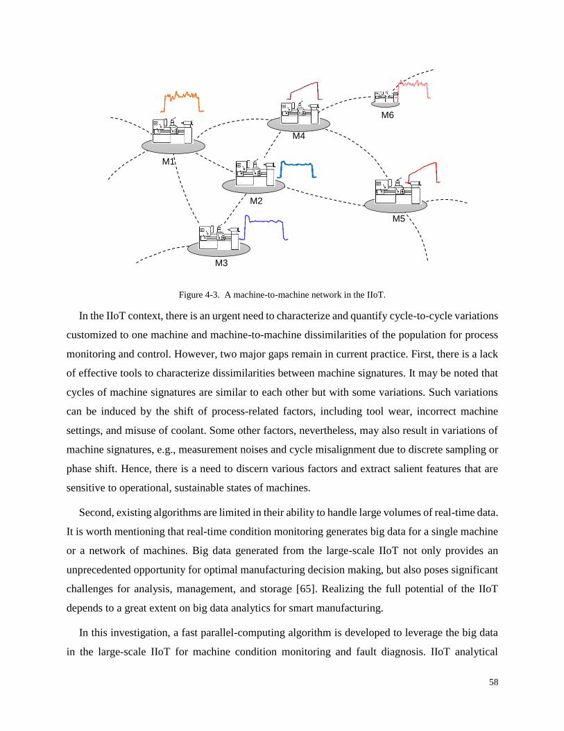
58
Figure 4-3. A machine-to-machine network in the IIoT.
In the IIoT context, there is an urgent need to characterize and quantify cycle-to-cycle variations
customized to one machine and machine-to-machine dissimilarities of the population for process
monitoring and control. However, two major gaps remain in current practice. First, there is a lack
of effective tools to characterize dissimilarities between machine signatures. It may be noted that
cycles of machine signatures are similar to each other but with some variations. Such variations
can be induced by the shift of process-related factors, including tool wear, incorrect machine
settings, and misuse of coolant. Some other factors, nevertheless, may also result in variations of
machine signatures, e.g., measurement noises and cycle misalignment due to discrete sampling or
phase shift. Hence, there is a need to discern various factors and extract salient features that are
sensitive to operational, sustainable states of machines.
Second, existing algorithms are limited in their ability to handle large volumes of real-time data.
It is worth mentioning that real-time condition monitoring generates big data for a single machine
or a network of machines. Big data generated from the large-scale IIoT not only provides an
unprecedented opportunity for optimal manufacturing decision making, but also poses significant
challenges for analysis, management, and storage [65]. Realizing the full potential of the IIoT
depends to a great extent on big data analytics for smart manufacturing.
In this investigation, a fast parallel-computing algorithm is developed to leverage the big data
in the large-scale IIoT for machine condition monitoring and fault diagnosis. IIoT analytical
M1
M2
M3
M4
M6
M5

59
methods and tools will enable and assist (i) the handling of massive data communicated by the
IIoT; (ii) the extraction of pertinent knowledge about machine dynamics; (iii) the exploitation of
acquired knowledge for data-driven analysis and performance optimization of machines.
Specifically, a dynamic time warping approach is introduced to measure dissimilarities among
machine signatures. Then, machines are optimally embedded into a network in the high-
dimensional space (e.g., 2D and 3D). Each node corresponds to one machine, and Euclidean
distances between network nodes preserve the dissimilarity of machine signatures. As such, the
location of network nodes reveals diagnostic features pertinent to machine conditions. However,
the ability to optimize a large network is hampered in traditional algorithms, due to their high
computational complexity. Thus, we further introduce a stochastic network embedding approach
to handle the large-scale machine network. Parallel-computing algorithms are also developed to
speed up the stochastic embedding approach. Experimental results show significant reduction of
running time for a large-scale IIoT network. Our contributions in the present investigation are
highlighted as follows:
1) We introduce a stochastic embedding approach (rather than traditional deterministic
algorithms) to significantly improve the computational efficiency of network embedding
and optimize the embedding of each machine in the network.
2) We develop a fast parallel algorithm (rather than traditional serial computing) to enable the
embedding of large-scale machine networks in the context of IIoT.
The remainder of this paper is organized as follows: Section 4.2 introduces the research
background in condition monitoring, IIoT, and parallel computing. Section 4.3 presents the
methodology of stochastic network embedding and parallel computing algorithms developed in
this research. Case studies and experimental results are shown in Section 4.4. Section 4.5 discusses
and concludes this research.
4.2. Research Background
A. Advanced Sensing and Condition Monitoring
Rapid advances in sensing technology have prompted the proliferation of advanced sensing in
manufacturing. 1) Instead of single-channel sensors, multi-channel sensors are more and more
adopted for the machine condition monitoring. By distributing sensors at different positions, multi-
channel sensing provides a comprehensive view of the manufacturing system. For example, four
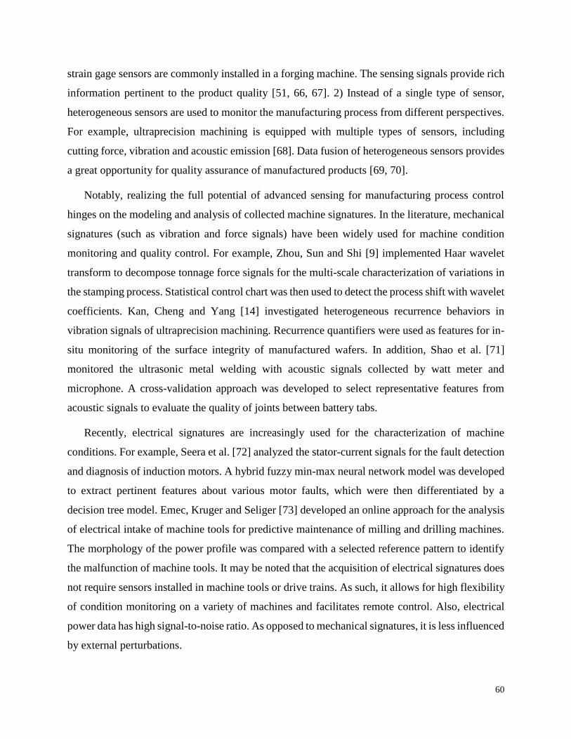
60
strain gage sensors are commonly installed in a forging machine. The sensing signals provide rich
information pertinent to the product quality [51, 66, 67]. 2) Instead of a single type of sensor,
heterogeneous sensors are used to monitor the manufacturing process from different perspectives.
For example, ultraprecision machining is equipped with multiple types of sensors, including
cutting force, vibration and acoustic emission [68]. Data fusion of heterogeneous sensors provides
a great opportunity for quality assurance of manufactured products [69, 70].
Notably, realizing the full potential of advanced sensing for manufacturing process control
hinges on the modeling and analysis of collected machine signatures. In the literature, mechanical
signatures (such as vibration and force signals) have been widely used for machine condition
monitoring and quality control. For example, Zhou, Sun and Shi [9] implemented Haar wavelet
transform to decompose tonnage force signals for the multi-scale characterization of variations in
the stamping process. Statistical control chart was then used to detect the process shift with wavelet
coefficients. Kan, Cheng and Yang [14] investigated heterogeneous recurrence behaviors in
vibration signals of ultraprecision machining. Recurrence quantifiers were used as features for in-
situ monitoring of the surface integrity of manufactured wafers. In addition, Shao et al. [71]
monitored the ultrasonic metal welding with acoustic signals collected by watt meter and
microphone. A cross-validation approach was developed to select representative features from
acoustic signals to evaluate the quality of joints between battery tabs.
Recently, electrical signatures are increasingly used for the characterization of machine
conditions. For example, Seera et al. [72] analyzed the stator-current signals for the fault detection
and diagnosis of induction motors. A hybrid fuzzy min-max neural network model was developed
to extract pertinent features about various motor faults, which were then differentiated by a
decision tree model. Emec, Kruger and Seliger [73] developed an online approach for the analysis
of electrical intake of machine tools for predictive maintenance of milling and drilling machines.
The morphology of the power profile was compared with a selected reference pattern to identify
the malfunction of machine tools. It may be noted that the acquisition of electrical signatures does
not require sensors installed in machine tools or drive trains. As such, it allows for high flexibility
of condition monitoring on a variety of machines and facilitates remote control. Also, electrical
power data has high signal-to-noise ratio. As opposed to mechanical signatures, it is less influenced
by external perturbations.

61
However, most previous approaches focus on the analysis of representative cycles from a
single machine. Very little has been done to characterize cycle-to-cycle and machine-to-machine
variations for machine condition monitoring in the context of large-scale IIoT. It may be noted that
continuous monitoring of machines as collaborative agents in a network will facilitate real-time
loading and maintenance scheduling, and thereby improving the productivity. Thus, there is a need
to design and develop new approaches that effectively leverage continuously collected IIoT data
for in-situ process monitoring and control.
B. Industrial Internet of Things
In the past few years, the manufacturing industry is hurtling into the era of IIoT [74]. By
connecting wireless sensors and mobile computing units, IIoT is triggering a paradigm shift in
manufacturing, and it will be a major trend for the global industry. Nowadays, a massive number
of machines and tools, from oil-drilling rigs to steel mills, are equipped with sensors to collect and
send data. Data analytics help to detect the operational issues and process anomalies in the
manufacturing system. Parts are automatically replenished, and machine tools are replaced before
failure occurs. As such, the IIoT significantly reduces the risk of unplanned outages and improves
the production throughput. It is estimated that IIoT-enabled predictive maintenance saves up to
12% of over scheduled repairs, reduces 30% maintenance costs, and eliminates breakdowns up to
70% [75].
In addition, a large-scale machine network can be established under the cyber-physical system
of IIoT. Machines are represented as nodes in the network, and the machine-to-machine
communication is realized through network arcs. Manufacturers can access the machines’
operational dynamics anywhere anytime via the machine network and deliver remote, even
overseas maintenance services. This will help reduce machine downtime and avoid shutdowns of
factories. Nowadays, manufacturers are identifying new growth opportunities by adding intelligent
products and digital services that communicate with each other and with people globally.
However, existing studies of the IIoT mainly focus on sensor development, wireless
communication and information architecture [76][77]. Few analytics algorithms have been
developed to leverage data collected in the IIoT for machine condition monitoring. There is a need
to develop efficient algorithms to characterize collected machine signatures and quantify salient

62
features that are sensitive to operational, environmental, and sustainable states of manufacturing
processes.
C. Serial Computing vs. Parallel Computing
Traditionally, analytics algorithms are implemented in the serial-computing framework. As
shown in Fig. 4-4a, serial computing decomposes the overall task (e.g., condition assessment of a
large group of machines) into a discrete series of sub-tasks (e.g. assess the condition of individual
machines). Then, sub-tasks are executed sequentially on a single processor. Although serial
computing is efficient for analyzing small datasets, the computational complexity may increase
exponentially with the growth of sample size, which results in prohibitive computation time. This,
in turn, significantly hampers the use of serial computing for big data analytics in large-scale IIoT.
Therefore, researchers are seeking a way to scale up the algorithm and utilize more computing
resources to complete a task collaboratively.
Rapid advancements in information technology have catalyzed the incredibly fast growth in
computing power. Recently, parallel computing has been employed to harness multiple processing
units to solve problems. As opposed to serial processing, parallel computing is achieved by
pipelining the overall task into multiple processors. As shown in Fig. 4-4b, each processor executes
its part of the computation and works simultaneously with other processors. As such, the
computing time can be critically reduced. Nowadays, the availability of multi-core CPUs, cell
processors (e.g., GPUs) and cloud computing technology make parallel computing easily
achievable by deploying off-the-shelf strategies such as multi-threaded and single-instruction-
multiple-data. Parallel computing has been widely used in various research areas, including
genetics, geology, medical imaging, and graph mining.
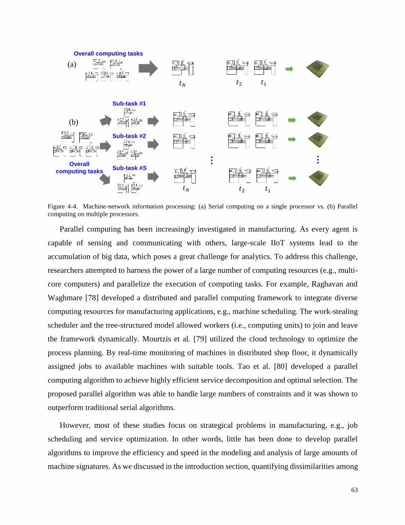
63
Figure 4-4. Machine-network information processing: (a) Serial computing on a single processor vs. (b) Parallel
computing on multiple processors.
Parallel computing has been increasingly investigated in manufacturing. As every agent is
capable of sensing and communicating with others, large-scale IIoT systems lead to the
accumulation of big data, which poses a great challenge for analytics. To address this challenge,
researchers attempted to harness the power of a large number of computing resources (e.g., multi-
core computers) and parallelize the execution of computing tasks. For example, Raghavan and
Waghmare [78] developed a distributed and parallel computing framework to integrate diverse
computing resources for manufacturing applications, e.g., machine scheduling. The work-stealing
scheduler and the tree-structured model allowed workers (i.e., computing units) to join and leave
the framework dynamically. Mourtzis et al. [79] utilized the cloud technology to optimize the
process planning. By real-time monitoring of machines in distributed shop floor, it dynamically
assigned jobs to available machines with suitable tools. Tao et al. [80] developed a parallel
computing algorithm to achieve highly efficient service decomposition and optimal selection. The
proposed parallel algorithm was able to handle large numbers of constraints and it was shown to
outperform traditional serial algorithms.
However, most of these studies focus on strategical problems in manufacturing, e.g., job
scheduling and service optimization. In other words, little has been done to develop parallel
algorithms to improve the efficiency and speed in the modeling and analysis of large amounts of
machine signatures. As we discussed in the introduction section, quantifying dissimilarities among
𝑡1 𝑡2 𝑡𝑁
(a)
Overall computing tasks
…
…
𝑡1 𝑡2 𝑡𝑁
(b)
Sub-task #1
Sub-task #2
Sub-task #S Overall
computing tasks
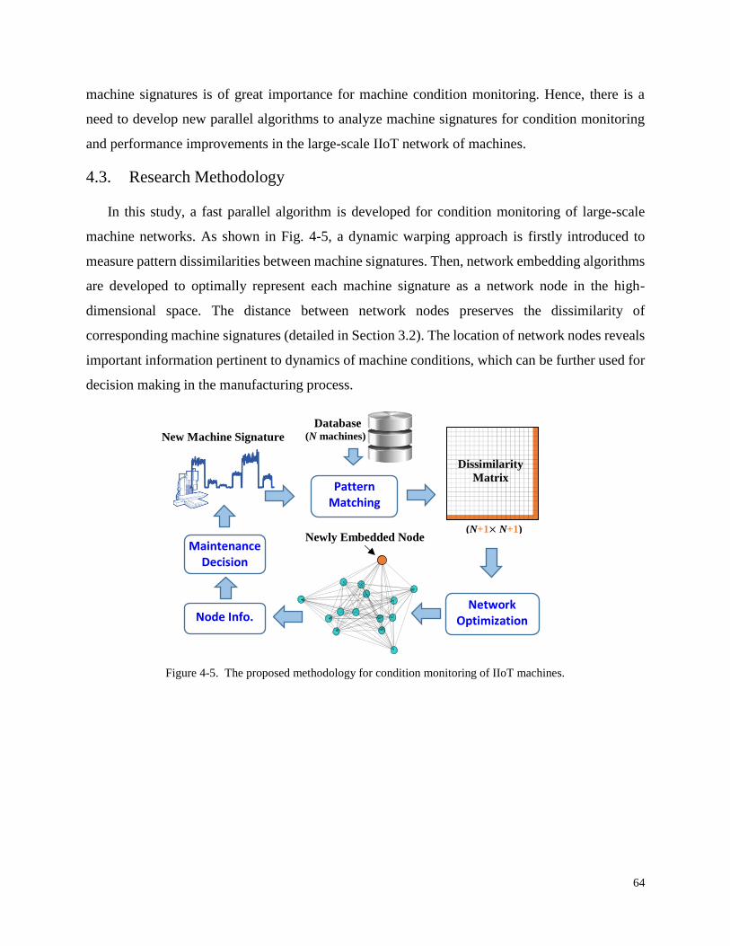
64
machine signatures is of great importance for machine condition monitoring. Hence, there is a
need to develop new parallel algorithms to analyze machine signatures for condition monitoring
and performance improvements in the large-scale IIoT network of machines.
4.3. Research Methodology
In this study, a fast parallel algorithm is developed for condition monitoring of large-scale
machine networks. As shown in Fig. 4-5, a dynamic warping approach is firstly introduced to
measure pattern dissimilarities between machine signatures. Then, network embedding algorithms
are developed to optimally represent each machine signature as a network node in the high-
dimensional space. The distance between network nodes preserves the dissimilarity of
corresponding machine signatures (detailed in Section 3.2). The location of network nodes reveals
important information pertinent to dynamics of machine conditions, which can be further used for
decision making in the manufacturing process.
Figure 4-5. The proposed methodology for condition monitoring of IIoT machines.
Pattern Matching
Database (N machines)
Network Optimization Node Info.
Maintenance Decision
(N+1× N+1)
Dissimilarity
Matrix
New Machine Signature
Newly Embedded Node
65
A. Pattern Matching and Signature Warping
Figure 4-6. Power consumptions of two turning processes.
As shown in Fig. 4-6, dissimilarities are found between two energy profiles turning processes.
The red profile consumes higher energy in the cutting phase, which indicates the potential tool
wear. Quantification of such dissimilarities will provide a great opportunity for condition
monitoring of machines and tools. Traditional methods focus on the comparison with reference
signatures (i.e., “standard” or “normal” ones). We propose to perform a pairwise comparison of
machine signatures in either cycle-to-cycle or machine-to-machine ways. Note that a dissimilarity
matrix (consists of the dissimilarity between each pair of signatures) is obtained from pairwise
comparison, rather than only a column in reference comparison.
However, two signatures can be misaligned due to discrete sampling and phase shift [40, 81].
For example, the blue and red signatures show a typical pattern, but there are variations in shape,
amplitude, and phase (see Fig. 4-6). Directly taking the Euclidean distances between two
misaligned signatures (e.g., Fig. 4-7a) will result in a large dissimilarity, even for phases that are
alike. Therefore, it is imperative to optimally align the profiles in terms of spindle and cutting
activities in different phases. For example, we should compare the cutting phases between two
signatures, as opposed to an incorrect comparison between the cutting of end surface (in red) and
spindle deceleration (in blue).
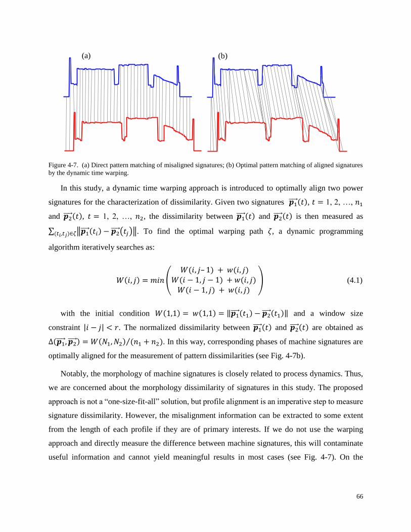
66
Figure 4-7. (a) Direct pattern matching of misaligned signatures; (b) Optimal pattern matching of aligned signatures
by the dynamic time warping.
In this study, a dynamic time warping approach is introduced to optimally align two power
signatures for the characterization of dissimilarity. Given two signatures 𝒑1⃗⃗⃗⃗ (𝑡), 𝑡 = 1, 2, …, 𝑛1
and 𝒑2⃗⃗ ⃗⃗ (𝑡), 𝑡 = 1, 2, …, 𝑛2, the dissimilarity between 𝒑1⃗⃗⃗⃗ (𝑡) and 𝒑2⃗⃗ ⃗⃗ (𝑡) is then measured as
∑ ‖𝒑1⃗⃗⃗⃗ (𝑡𝑖) − 𝒑2⃗⃗ ⃗⃗ (𝑡𝑗)‖(𝑡𝑖,𝑡𝑗)∈𝜁 . To find the optimal warping path 𝜁, a dynamic programming
algorithm iteratively searches as:
𝑊(𝑖, 𝑗) = 𝑚𝑖𝑛 (
𝑊(𝑖, 𝑗– 1) + 𝑤(𝑖, 𝑗)𝑊(𝑖 − 1, 𝑗 − 1) + 𝑤(𝑖, 𝑗)
𝑊(𝑖 − 1, 𝑗) + 𝑤(𝑖, 𝑗) ) (4.1)
with the initial condition 𝑊(1,1) = 𝑤(1,1) = ‖𝒑1⃗⃗⃗⃗ (𝑡1) − 𝒑2⃗⃗ ⃗⃗ (𝑡1)‖ and a window size
constraint |𝑖 − 𝑗| < 𝑟. The normalized dissimilarity between 𝒑1⃗⃗⃗⃗ (𝑡) and 𝒑2⃗⃗ ⃗⃗ (𝑡) are obtained as
∆(𝒑1⃗⃗⃗⃗ , 𝒑2⃗⃗ ⃗⃗ ) = 𝑊(𝑁1, 𝑁2) (𝑛1 + 𝑛2)⁄ . In this way, corresponding phases of machine signatures are
optimally aligned for the measurement of pattern dissimilarities (see Fig. 4-7b).
Notably, the morphology of machine signatures is closely related to process dynamics. Thus,
we are concerned about the morphology dissimilarity of signatures in this study. The proposed
approach is not a “one-size-fit-all” solution, but profile alignment is an imperative step to measure
signature dissimilarity. However, the misalignment information can be extracted to some extent
from the length of each profile if they are of primary interests. If we do not use the warping
approach and directly measure the difference between machine signatures, this will contaminate
useful information and cannot yield meaningful results in most cases (see Fig. 4-7). On the
(a) (b)
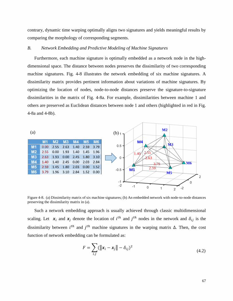
67
contrary, dynamic time warping optimally aligns two signatures and yields meaningful results by
comparing the morphology of corresponding segments.
B. Network Embedding and Predictive Modeling of Machine Signatures
Furthermore, each machine signature is optimally embedded as a network node in the high-
dimensional space. The distance between nodes preserves the dissimilarity of two corresponding
machine signatures. Fig. 4-8 illustrates the network embedding of six machine signatures. A
dissimilarity matrix provides pertinent information about variations of machine signatures. By
optimizing the location of nodes, node-to-node distances preserve the signature-to-signature
dissimilarities in the matrix of Fig. 4-8a. For example, dissimilarities between machine 1 and
others are preserved as Euclidean distances between node 1 and others (highlighted in red in Fig.
4-8a and 4-8b).
Figure 4-8. (a) Dissimilarity matrix of six machine signatures; (b) An embedded network with node-to-node distances
preserving the dissimilarity matrix in (a).
Such a network embedding approach is usually achieved through classic multidimensional
scaling. Let 𝒙𝑖 and 𝒙𝑗 denote the location of 𝑖𝑡ℎ and 𝑗𝑡ℎ nodes in the network and 𝛿𝑖𝑗 is the
dissimilarity between 𝑖𝑡ℎ and 𝑗𝑡ℎ machine signatures in the warping matrix ∆. Then, the cost
function of network embedding can be formulated as:
𝐹 = ∑(‖𝒙𝑖 − 𝒙𝑗‖ − 𝛿𝑖𝑗)2
𝑖,𝑗
(4.2)
M1 M5
M4 M3
M2
M6
2.55 1.40 2.63
3.79 2.59
(a) (b)
68
To optimize the location of network nodes, a Gram matrix B is reconstructed from dissimilarity
matrix ∆ as B = −1
2𝐻∆(2)𝐻, where H = 𝐼 − 𝑁−1𝟏𝟏𝑇 is a centering matrix. The element 𝑏𝑖𝑗 in
matrix B is obtained as:
𝑏𝑖𝑗 = −1
2[𝛿𝑖𝑗
2 −1
𝑁∑ 𝛿𝑖𝑘
2
𝑁
𝑘=1
−1
𝑁∑ 𝛿𝑘𝑗
2
𝑁
𝑘=1
+1
𝑁2∑ ∑ 𝛿𝑔ℎ
2
𝑁
ℎ=1
𝑁
𝑔=1
] (4.3)
The Gram matrix B can be defined as the scalar product 𝐵 = 𝑋𝑋𝑇, which is further written as
B = 𝑉𝛬𝑉𝑇 = 𝑉√𝛬√𝛬𝑉𝑇 by eigen-decomposition [81]. Here, 𝑉 is a matrix of eigenvectors and 𝛬
is a diagonal matrix of eigenvalues. Hence, optimal coordinates of network nodes are obtained
as: 𝑋 = 𝑉√𝛬.
As a result, each machine signature is represented as a node in the network. Euclidean distances
between nodes preserve warping distances, thereby characterizing signature-to-signature
variations in the manufacturing process. This, in turn, allows the use of network information (e.g.,
coordinates of nodes) as features for condition monitoring and predictive modeling. 1) For the
monitoring of cycle-to-cycle variations of a single machine, each node is embedded from one
operation cycle of machine signature. If embedded nodes are located apart from the cluster of
normal condition, maintenance service needs to be scheduled to prevent machine failure. 2) For
the analysis of a machine network, each node represents a machine or the signature (e.g., power
profiles, features, or patterns) of the machine. Classification models can be constructed to predict
the machine condition based on coordinates of the corresponding node. If the machine condition
is more likely to be abnormal, engineers can re-assign its jobs to other machines and schedule the
maintenance. In our previous studies, various predictive modeling approaches were developed,
including linear and quadratic discriminant models [8], neural networks [81], self-organizing
networks [82], and particle filtering [83]. Practitioners can select an optimal predictive modeling
approach based on the complexity of data and requirements of processing speed.
C. New Algorithms for Large-scale Network Modeling
1) Stochastic network embedding – serial computing algorithm
However, classic multidimensional scaling is limited in its ability to handle large volumes of
data. In other words, the computation time will be significantly increased when large numbers of
69
machines are involved in the network (e.g., 𝑁 >5,000). This is because the computational
complexity of classical multidimensional scaling is 𝑂(𝑁3), due to the centering operation and
eigen-decomposition. In fact, most of traditional algorithms for network embedding are limited in
the ability to handle big data due to high level of computational complexity. In addition to classic
multidimensional scaling, another example is scaling by majorizing of a complicated function
(SMACOF) [84]. It may be noted that SMACOF requires Guttman transform, which consists of a
multiplication between an 𝑁 × 𝑁 matrix and an 𝑁 × 𝐿 matrix (𝐿 is the dimensionality of the
network space). As such, it is difficult to use traditional algorithms for the optimization of a large-
scale machine network.
Notably, big data poses two significant challenges for optimization. On one hand, the
dimensionality of the data is high. As such, second order optimization is sometimes prohibitive.
Thus, first order methods are preferred, e.g., gradient-based method. On the other hand, large
volumes of data make it impractical for algorithms to scan the entire dataset many times. Hence,
a stochastic approach is better suited to handle big data, because only one data sample is considered
at every iteration. Moreover, it has been shown that the convergence of stochastic approaches for
the optimization of convex functions is guaranteed in most cases. Therefore, a stochastic
embedding approach is introduced to extend the integrated framework in Section 3.1 to large-scale
machine networks.
Motivated by [85], the objective function of network optimization in Eq. (4.2) is redefined as:
𝐹 =1
2∑∑(‖𝒙𝑖 − 𝒙𝑗‖ − 𝛿𝑖𝑗)
2
𝑗≠𝑖𝑖
𝛹(‖𝒙𝑖 − 𝒙𝑗‖, 𝜆) (4.4)
where 𝛹(∙) is a bounded and monotonically decreasing function to favor the local topology in the
network [85]. One example of 𝛹(∙) is a step function:
𝛹(‖𝒙𝑖 − 𝒙𝑗‖, 𝜆) = {1 if ‖𝒙𝑖 − 𝒙𝑗‖ ≤ 𝜆
0 if ‖𝒙𝑖 − 𝒙𝑗‖ > 𝜆 (4.5)
and 𝜆 is defines the neighborhood radius. Minimization of Eq. (4.4) with respect to 𝒙𝑗’s identifies
the optimal location of network nodes that preserve the signature-to-signature dissimilarity
measures. Notably, the decrease of 𝐹 values can be considered as a summation of partial decrease
generated by adjusting the location of each network node 𝑖, i.e., 𝐹 =1
2∑ 𝐹𝑖𝑖 . The optimization of

70
Eq. (4.4) works as follows: in each iteration, a node 𝑖 is randomly selected and its location (e.g.,
𝒙𝑖) is fixed. Then, all other nodes 𝒙𝑗(𝑗 ≠ 𝑖) are updated based on the following rule:
𝒙𝑗 ← 𝒙𝑗 − 𝜂𝑡
𝜕𝐹𝑖
𝜕𝒙𝑗 (4.6)
where the learning rate 𝜂𝑡 is monotonically deceasing over time. Different forms of 𝜂𝑡 can be used
and we adopt an exponential function:
𝜂𝑡 = 𝜂0 (𝜂𝑇
𝜂0)𝑡
(4.7)
where constants 𝜂0 and 𝜂𝑇 specify the initial and final scales of the learning rate and the ratio of 𝜂𝑇
and 𝜂0 determines the decaying speed. Furthermore, a similar form of exponential function can be
applied to shrink the radius of neighborhood 𝜆 in the learning process, which generates a
monotonically decreasing function 𝜆𝑡 = 𝜆0 (𝜆𝑇
𝜆0)𝑡
.
Proposition: The updating rule of stochastic network embedding is given as
{𝒙𝑗 ← 𝒙𝑗 − 𝜂𝑡
‖𝒙𝑖 − 𝒙𝑗‖ − 𝛿𝑖𝑗
‖𝒙𝑖 − 𝒙𝑗‖ (𝒙𝑗 − 𝒙𝑖) if ‖𝒙𝑖 − 𝒙𝑗‖ ≤ 𝜆𝑡
𝒙𝑗 is not updated if ‖𝒙𝑖 − 𝒙𝑗‖ > 𝜆𝑡
(4.8)
Proof: Introduce an auxiliary parameter: 𝐷𝑖𝑗 = ‖𝒙𝑖 − 𝒙𝑗‖ = √∑ (𝑥𝑖ℎ − 𝑥𝑗ℎ)2𝑝
ℎ=1 . According
to Eq. (4.4), 𝐹𝑖 can be written as 1
2∑ (𝐷𝑖𝑗 − 𝛿𝑖𝑗)
2𝛹(𝐷𝑖𝑗, 𝜆)𝑗 . Furthermore,
𝜕𝛹
𝜕𝒙𝑗= 1, if 𝐷𝑖𝑗 ≤ 𝜆𝑡.
Otherwise, 𝜕𝛹
𝜕𝒙𝑗= 0.
According to the chain rule:
𝜕𝐹𝑖
𝜕𝒙𝑗=
𝜕𝐹𝑖
𝜕𝐷𝑖𝑗 ∙
𝜕𝐷𝑖𝑗
𝜕𝒙𝑗
𝜕𝐹𝑖
𝜕𝐷𝑖𝑗=
1
2
𝜕 (∑ (𝐷𝑖𝑗 − 𝛿𝑖𝑗)2
𝑗 )
𝜕𝐷𝑖𝑗=
1
2
𝜕(∑ (𝐷𝑖𝑗2 − 2𝐷𝑖𝑗𝛿𝑖𝑗 + 𝛿𝑖𝑗
2)𝑗 )
𝜕𝐷𝑖𝑗= 𝐷𝑖𝑗 − 𝛿𝑖𝑗
Also we have:

71
𝜕𝐷𝑖𝑗
𝜕𝑥𝑗ℎ=
𝜕√∑ (𝑥𝑖ℎ − 𝑥𝑗ℎ)2𝑝
ℎ=1
𝜕𝑥𝑗ℎ=
1
2√∑ (𝑥𝑖ℎ − 𝑥𝑗ℎ)2𝑝
ℎ=1
∙ 𝜕 (∑ (𝑥𝑖ℎ − 𝑥𝑗ℎ)
2𝑝ℎ=1 )
𝜕𝑥𝑗ℎ
= 1
2𝐷𝑖𝑗 2(𝑥𝑗ℎ − 𝑥𝑖ℎ)
= 𝑥𝑗ℎ − 𝑥𝑖ℎ
𝐷𝑖𝑗
Thus,
𝜕𝐷𝑖𝑗
𝜕𝒙𝑗= (
𝜕𝐷𝑖𝑗
𝜕𝑥𝑗1,𝜕𝐷𝑖𝑗
𝜕𝑥𝑗2, … ,
𝜕𝐷𝑖𝑗
𝜕𝑥𝑗ℎ, … ) = (
𝑥𝑗1 − 𝑥𝑖1
𝐷𝑖𝑗,𝑥𝑗2 − 𝑥𝑖2
𝐷𝑖𝑗, … ,
𝑥𝑗ℎ − 𝑥𝑖ℎ
𝐷𝑖𝑗, … ) =
𝒙𝑗 − 𝒙𝑖
𝐷𝑖𝑗
Therefore:
𝜕𝐹𝑖
𝜕𝒙𝑗=
(‖𝒙𝑖 − 𝒙𝑗‖ − 𝛿𝑖𝑗) (𝒙𝑗 − 𝒙𝑖)
‖𝒙𝑖 − 𝒙𝑗‖
and substitute it into Eq. (4.6), we have Eq. (4.8). ∎
This approach iterates until the maximum number of learning epoch is reached. Notably, the
update rule in Eq. (4.8) can be done by matrix operation and vectorization. In other words, the
location of all other nodes (i.e., 𝒙𝑗(𝑗 ≠ 𝑖)) are simultaneously updated instead of one by one, which
accelerates the update process. The stochastic embedding approach is summarized in Algorithm 4-
1.
Algorithm 4-1 Stochastic network embedding – serial computing
Input: dissimilarity matrix ∆ (𝛿𝑖𝑗)
Output: coordinates of nodes 𝒙𝑖, 𝑖 ∈ {1, 2, … ,𝑁} in the high-dimensional network
1: 𝑇 – number of epochs
2: initialize 𝒙𝑖, learning rate {𝜂𝑡}𝑡=1𝑇 and neighborhood radius {𝜆𝑡}𝑡=1
𝑇
3: for 𝑡 =1, 2, …, 𝑇 do
4: create index sequence 𝜗 by random permutation of {1, 2, … ,𝑁} 5: for 𝑛 = 1 to 𝑁 do
6: draw 𝑖 ∈ 𝜗 , fix the 𝒙𝑖
7: update using Eq. (4.8)
8: end for
9: end for
2) Stochastic network embedding – new parallel computing algorithm
Algorithm 1 processes one node per iteration and the computational complexity in each
iteration is low. However, it takes a long time for Algorithm 1 to find the optimal solution when a
large number of machines or production cycles of a machine are involved. Thus, it is imperative
to parallelize the algorithm and utilize more computing resources collaboratively. However, the

72
inherently sequential nature of Algorithm 1 poses significant challenges for parallelization. An
algorithm can be parallelized if the computing task can be decomposed and results from individual
processors (or computers) are independent of each other. Notably, fixing the location of nodes 𝑎
or 𝑏 and updating the location of other nodes will result in different locations of 𝑐 especially when
𝑎 and 𝑏 are far from each other. Thus, Algorithm 1 is difficult to be parallelized.
To address this challenge, one practical solution is to combine stochastic embedding with batch
learning, which results in the mini-batch stochastic embedding. Instead of considering one sample
at a time, the mini-batch stochastic embedding considers multiple samples (i.e., a mini-batch)
simultaneously at each iteration [86]. Assume the total number of data 𝑁 can be partitioned into
𝑀 mini-batches, each of the size 𝑚. Given a randomly selected mini-batch 𝛾𝑡 ⊂ {1, 2, … ,𝑁}, the
objective function on the mini-batch can be written as 𝐹𝛾𝑡=
1
|𝛾𝑡|∑ 𝐹𝑖𝑖∈𝛾𝑡
, where |𝛾𝑡| = 𝑚 is the size
of a batch. At each iteration, the mini-batch stochastic embedding accumulates sub-gradients with
respect to 𝑚 samples in the batch and calculate the average gradients as:
∇𝐹𝛾𝑡=
1
|𝛾𝑡|∑ ∇𝐹𝑖
𝑖∈𝛾𝑡
(4.9)
where ∇𝐹𝑖 =𝜕𝐹𝑖
𝜕𝒙𝑗. As such, each mini-batch generates a single average gradient. At the end of each
batch, mini-batch stochastic embedding feeds ∇𝐹𝛾𝑡 to update the location of all other nodes 𝒙𝑗 (𝑗 ≠
𝑖) as:
𝒙𝑗 ← 𝒙𝑗 − 𝜂𝑡∇𝐹𝛾𝑡 (4.10)
Therefore, the update rule of Eq. (4.8) can be rewritten as:
{𝒙𝑗 ← 𝒙𝑗 − 𝜂𝑡
1
|𝛾𝑡|∑
‖𝒙𝑖 − 𝒙𝑗‖ − 𝛿𝑖𝑗
‖𝒙𝑖 − 𝒙𝑗‖ (𝒙𝑗 − 𝒙𝑖)
𝑖∈𝛾𝑡
if ‖𝒙𝑖 − 𝒙𝑗‖ ≤ 𝜆𝑡
𝒙𝑗 is not updated if ‖𝒙𝑖 − 𝒙𝑗‖ > 𝜆𝑡
(4.11)
It may be noted that Eq. (4.11) is equivalent to Eq. (4.8) when the size of batch 𝑚 = 1. As the
update is executed less frequently, the mini-batch stochastic embedding provides computational
benefits.

73
Further, each mini-batch can be further considered as a combination of multiple subsets, i.e.,
𝛾𝑡 = 𝛾𝑡,1 ∪ 𝛾𝑡,2 ∪,… ,∪ 𝛾𝑡,𝑆. Thus, the calculation of sub-gradients in Eq. (4.9) can be further
represented as:
∇𝐹𝛾𝑡=
1
|𝛾𝑡|∑ ∇𝐹𝑖
𝑖∈𝛾𝑡
=1
|𝛾𝑡|[∑ ∇𝐹𝑖
𝑖∈𝛾𝑡,1
+ ∑ ∇𝐹𝑖𝑖∈𝛾𝑡,2
+ ⋯+ ∑ ∇𝐹𝑖𝑖∈𝛾𝑡,𝑆
] (4.12)
As a result, the mini-batch stochastic embedding can be readily implemented in a parallel
manner. That is, the mini- batch 𝛾𝑡 can be divided and the computation of average gradient can be
assigned to 𝑆 individual processors. Each processor s will compute ∑ ∇𝐹𝑖𝑖∈𝛾𝑡.𝑠 and results from 𝑆
processors are combined using Eq. (4.12) to return the average gradient with respect to all 𝑚
samples in the mini-batch. The parallel stochastic network embedding algorithm is summarized in
Algorithm 4-2.
Algorithm 4-2 Stochastic network embedding – parallel computing
1: initialize as Algorithm 4-1 step 1 and 2
2: randomly partition data into 𝑀 mini-batch 𝛾1, 𝛾2, …, 𝛾𝑀
3: start parallel pool with 𝑆 processors
4: for 𝑡 =1, 2, …, 𝑇 do
5: randomly choose a mini-batch 𝛾𝑡
6: partition 𝛾𝑡 into subsets 𝛾𝑡,1, 𝛾𝑡,2,…, 𝛾𝑡,𝑆, each with size 𝑚
7: for 𝑛 = 1 to 𝑀 do {in parallel}
8: processor # s gets partition 𝛾𝑡,𝑠
9: solve the sub-problem ∇𝐹𝑖∈𝛾𝑡,𝑠 on 𝛾𝑡,𝑠 by Algorithm 1
10: end for
11: average over the batch size 𝑚 and update 𝒙𝑗
12: end for
13: close parallel pool
4.4. Experiments and Results
In the present investigation, we evaluate the proposed methodology in the development of a
large-scale machine-to-machine network, as well as a cycle-to-cycle network for the monitoring
of machine conditions. First, we compare the performance of our proposed parallel algorithm over
traditional approaches for handling a large machine network. Second, the proposed methodology
is implemented for the development of a cycle-to-cycle network customized to one machine.
Power profiles are simulated and used in experimental studies to characterize dynamics of the
underlying machining process. Our experiments and results are detailed in the following sections.
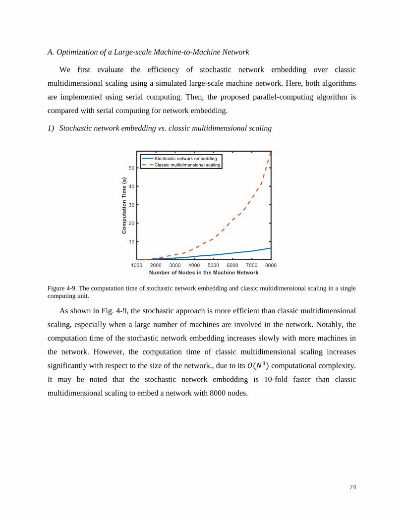
74
A. Optimization of a Large-scale Machine-to-Machine Network
We first evaluate the efficiency of stochastic network embedding over classic
multidimensional scaling using a simulated large-scale machine network. Here, both algorithms
are implemented using serial computing. Then, the proposed parallel-computing algorithm is
compared with serial computing for network embedding.
1) Stochastic network embedding vs. classic multidimensional scaling
Figure 4-9. The computation time of stochastic network embedding and classic multidimensional scaling in a single
computing unit.
As shown in Fig. 4-9, the stochastic approach is more efficient than classic multidimensional
scaling, especially when a large number of machines are involved in the network. Notably, the
computation time of the stochastic network embedding increases slowly with more machines in
the network. However, the computation time of classic multidimensional scaling increases
significantly with respect to the size of the network., due to its 𝑂(𝑁3) computational complexity.
It may be noted that the stochastic network embedding is 10-fold faster than classic
multidimensional scaling to embed a network with 8000 nodes.
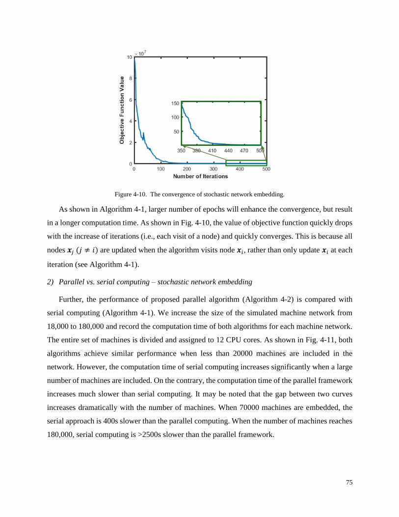
75
Figure 4-10. The convergence of stochastic network embedding.
As shown in Algorithm 4-1, larger number of epochs will enhance the convergence, but result
in a longer computation time. As shown in Fig. 4-10, the value of objective function quickly drops
with the increase of iterations (i.e., each visit of a node) and quickly converges. This is because all
nodes 𝒙𝑗 (𝑗 ≠ 𝑖) are updated when the algorithm visits node 𝒙𝑖, rather than only update 𝒙𝑖 at each
iteration (see Algorithm 4-1).
2) Parallel vs. serial computing – stochastic network embedding
Further, the performance of proposed parallel algorithm (Algorithm 4-2) is compared with
serial computing (Algorithm 4-1). We increase the size of the simulated machine network from
18,000 to 180,000 and record the computation time of both algorithms for each machine network.
The entire set of machines is divided and assigned to 12 CPU cores. As shown in Fig. 4-11, both
algorithms achieve similar performance when less than 20000 machines are included in the
network. However, the computation time of serial computing increases significantly when a large
number of machines are included. On the contrary, the computation time of the parallel framework
increases much slower than serial computing. It may be noted that the gap between two curves
increases dramatically with the number of machines. When 70000 machines are embedded, the
serial approach is 400s slower than the parallel computing. When the number of machines reaches
180,000, serial computing is >2500s slower than the parallel framework.
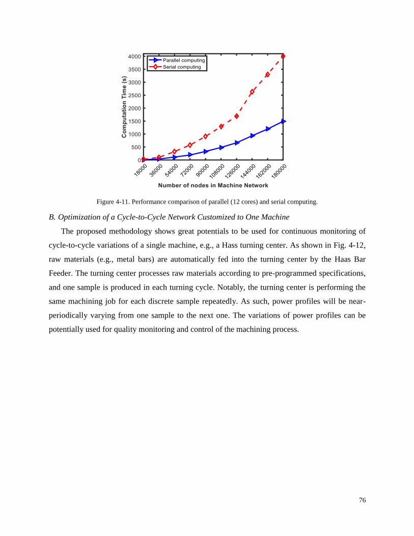
76
Figure 4-11. Performance comparison of parallel (12 cores) and serial computing.
B. Optimization of a Cycle-to-Cycle Network Customized to One Machine
The proposed methodology shows great potentials to be used for continuous monitoring of
cycle-to-cycle variations of a single machine, e.g., a Hass turning center. As shown in Fig. 4-12,
raw materials (e.g., metal bars) are automatically fed into the turning center by the Haas Bar
Feeder. The turning center processes raw materials according to pre-programmed specifications,
and one sample is produced in each turning cycle. Notably, the turning center is performing the
same machining job for each discrete sample repeatedly. As such, power profiles will be near-
periodically varying from one sample to the next one. The variations of power profiles can be
potentially used for quality monitoring and control of the machining process.
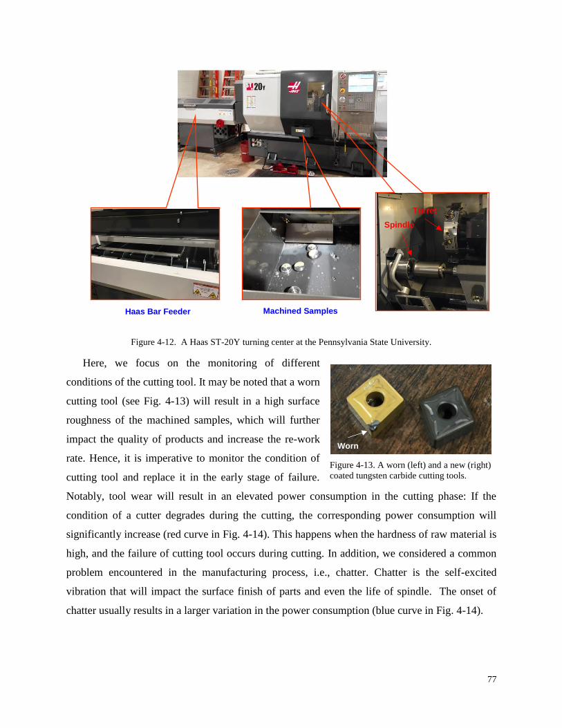
77
Figure 4-12. A Haas ST-20Y turning center at the Pennsylvania State University.
Here, we focus on the monitoring of different
conditions of the cutting tool. It may be noted that a worn
cutting tool (see Fig. 4-13) will result in a high surface
roughness of the machined samples, which will further
impact the quality of products and increase the re-work
rate. Hence, it is imperative to monitor the condition of
cutting tool and replace it in the early stage of failure.
Notably, tool wear will result in an elevated power consumption in the cutting phase: If the
condition of a cutter degrades during the cutting, the corresponding power consumption will
significantly increase (red curve in Fig. 4-14). This happens when the hardness of raw material is
high, and the failure of cutting tool occurs during cutting. In addition, we considered a common
problem encountered in the manufacturing process, i.e., chatter. Chatter is the self-excited
vibration that will impact the surface finish of parts and even the life of spindle. The onset of
chatter usually results in a larger variation in the power consumption (blue curve in Fig. 4-14).
Haas Bar Feeder Machined Samples
Spindle
Turret
Figure 4-13. A worn (left) and a new (right)
coated tungsten carbide cutting tools.
Worn
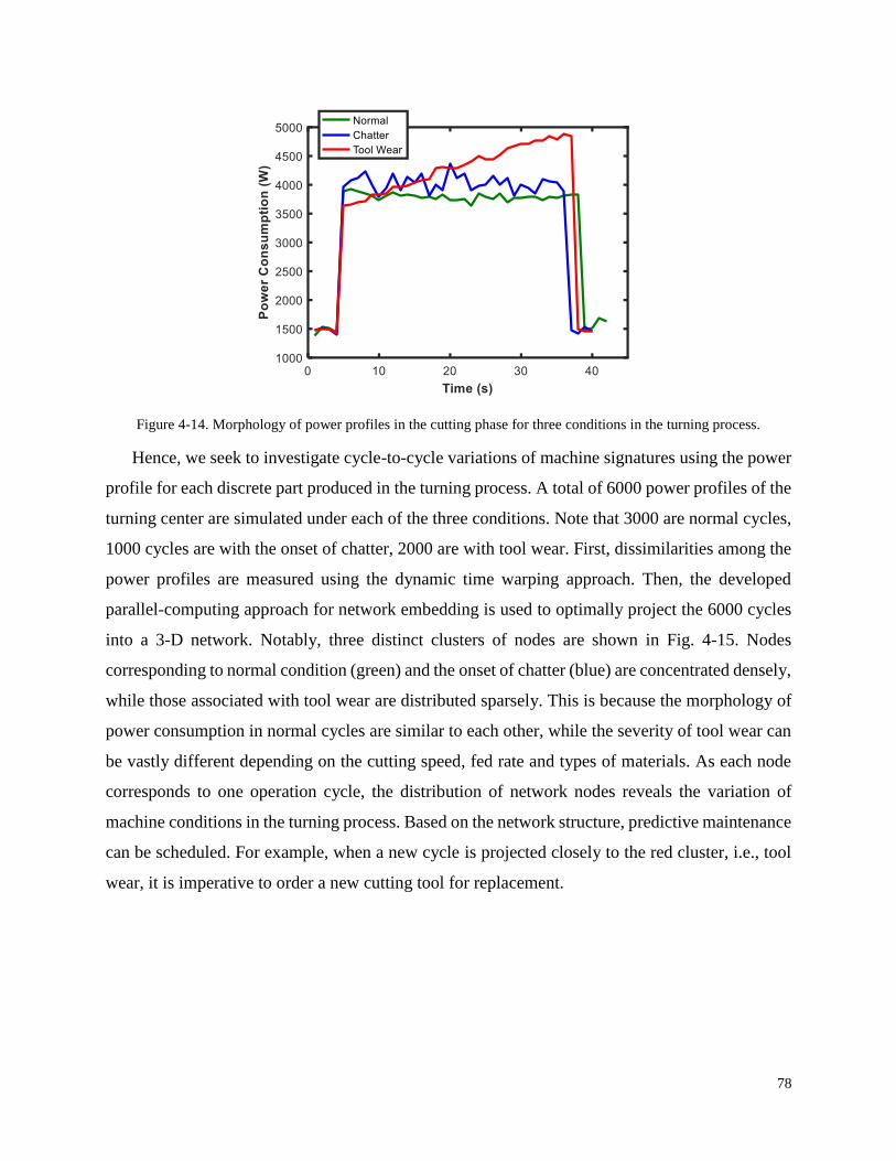
78
Figure 4-14. Morphology of power profiles in the cutting phase for three conditions in the turning process.
Hence, we seek to investigate cycle-to-cycle variations of machine signatures using the power
profile for each discrete part produced in the turning process. A total of 6000 power profiles of the
turning center are simulated under each of the three conditions. Note that 3000 are normal cycles,
1000 cycles are with the onset of chatter, 2000 are with tool wear. First, dissimilarities among the
power profiles are measured using the dynamic time warping approach. Then, the developed
parallel-computing approach for network embedding is used to optimally project the 6000 cycles
into a 3-D network. Notably, three distinct clusters of nodes are shown in Fig. 4-15. Nodes
corresponding to normal condition (green) and the onset of chatter (blue) are concentrated densely,
while those associated with tool wear are distributed sparsely. This is because the morphology of
power consumption in normal cycles are similar to each other, while the severity of tool wear can
be vastly different depending on the cutting speed, fed rate and types of materials. As each node
corresponds to one operation cycle, the distribution of network nodes reveals the variation of
machine conditions in the turning process. Based on the network structure, predictive maintenance
can be scheduled. For example, when a new cycle is projected closely to the red cluster, i.e., tool
wear, it is imperative to order a new cutting tool for replacement.
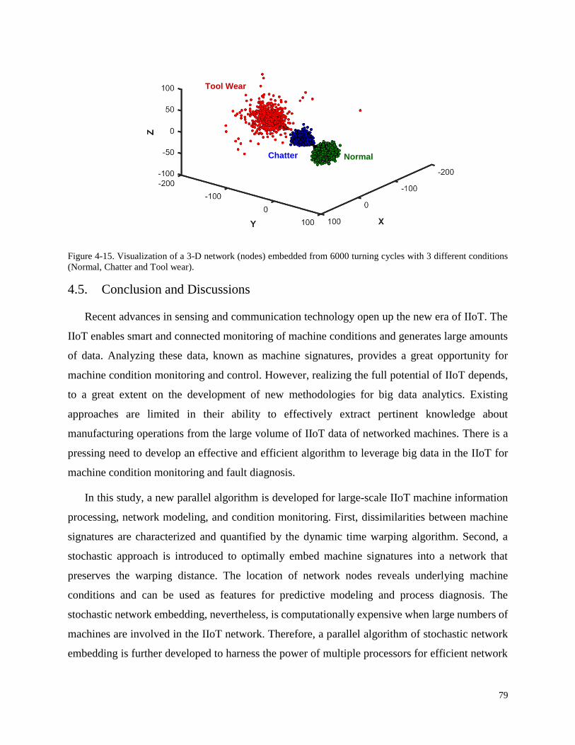
79
Figure 4-15. Visualization of a 3-D network (nodes) embedded from 6000 turning cycles with 3 different conditions
(Normal, Chatter and Tool wear).
4.5. Conclusion and Discussions
Recent advances in sensing and communication technology open up the new era of IIoT. The
IIoT enables smart and connected monitoring of machine conditions and generates large amounts
of data. Analyzing these data, known as machine signatures, provides a great opportunity for
machine condition monitoring and control. However, realizing the full potential of IIoT depends,
to a great extent on the development of new methodologies for big data analytics. Existing
approaches are limited in their ability to effectively extract pertinent knowledge about
manufacturing operations from the large volume of IIoT data of networked machines. There is a
pressing need to develop an effective and efficient algorithm to leverage big data in the IIoT for
machine condition monitoring and fault diagnosis.
In this study, a new parallel algorithm is developed for large-scale IIoT machine information
processing, network modeling, and condition monitoring. First, dissimilarities between machine
signatures are characterized and quantified by the dynamic time warping algorithm. Second, a
stochastic approach is introduced to optimally embed machine signatures into a network that
preserves the warping distance. The location of network nodes reveals underlying machine
conditions and can be used as features for predictive modeling and process diagnosis. The
stochastic network embedding, nevertheless, is computationally expensive when large numbers of
machines are involved in the IIoT network. Therefore, a parallel algorithm of stochastic network
embedding is further developed to harness the power of multiple processors for efficient network
Tool Wear
Chatter Normal

80
modeling of a large-scale IIoT machines. It may be noted that the proposed approach provides a
great opportunity for:
a) Dimensionality reduction: The network approach represents each power profile as a node
in the network based on the pairwise dissimilarity measures, which greatly reduced the
dimensionality of data and thereby identifies the “best data” to represent the machine
condition.
b) Visual analytics: The proposed approach provides a network representation of large
amounts of machines and further groups machines with similar conditions into
homogeneous clusters. This enables visual analytics of the data for condition monitoring of
machines. For example, we can pinpoint each profile from a machine in the network clusters
for monitoring or classification purposes.
c) High-performance computing: As a vertical step to improve computational efficiency, we
developed the stochastic network approach and parallelized the algorithm into multiple
processors to reduce computational complexity. In this way, the “best data” can be
efficiently identified for machine condition monitoring and performance improvement.
Notably, most traditional methods focus on the conformance to reference signatures (i.e.,
“standard” or “normal” ones). However, our method performs a pairwise comparison of signatures.
It may be noted that a dissimilarity matrix (consists of the dissimilarity between each pair of
signatures) is obtained from the pairwise comparison, rather than only a column in reference
comparison. For traditional reference comparison, the workload of computation is low, and it is
easy to implement. The difference against the reference can be directly used as an indicator to
determine if the current signature is normal or not. However, there is a need to empirically and/or
statistically establish a “normal” signature from a historical record of signatures. However, even
under the “normal” condition, the morphology of machine signatures may vary. Thus, it is difficult
to use one signature to represent the “normal” condition. On the contrary, there is no need for our
pairwise comparison to establish a “normal” signature. Instead, we develop a data-driven network
approach that leverages the pairwise dissimilarity information to automatically group large
amounts of signatures into homogeneous clusters. As such, the proposed network approach
provides a better representation of information in the data and further offers a great opportunity
for visual analytics of machine conditions. However, the workload of pairwise computation is
large. Also, it is challenging to extract information from the resulted dissimilarity matrix. In fact,

81
this motivates the development of an efficient and effective approach (i.e., fast parallel stochastic
network embedding) to fully utilize the pairwise comparison results for machine condition
monitoring.
This paper presents a pilot study on the development of cycle-to-cycle network for the purpose
of quality monitoring. In other words, one machine repeatedly manufactures the same type of
product in large quantities (the high volume, low mix scenario). Also, the cycle-to-cycle network
can be established from a large number of profiles pertinent to different types of parts. For
example, if there are two different kinds of parts, then power profiles from the same part tend to
have a higher level of similarity than those from a different part. This will lead to another
application of product classification. That is, network models leverage pairwise dissimilarity
measures to group profiles from the same part into a homogeneous cluster. Node location in the
network reveals useful information on the type of parts in production. Network visualization will
provide the categorization of parts, the evaluation of energy consumption, and further help
production planning. For the low volume high mix scenario, network models are not for quality
monitoring but rather can be used for potential applications to classify part or process
characteristics (e.g., types of materials, machining procedures, and specific tools used). For
example, the cycle-to-cycle network on the same machine can be used for product categorization
and energy monitoring. The machine-to-machine network can help extract useful information on
machine utilization, power usage, and condition monitoring, which will help further optimize
factory operations, reduce equipment downtime and maintenance costs.
To the best of our knowledge and review, little has been done to develop new methodologies
of parallel computing and network analytics for quality monitoring and control of large-scale IIoT
machines. The proposed methodology has a strong potential to promote existing manufacturing
practices towards globalized production optimization and management. Furthermore, it provides
a great opportunity to optimize the energy consumption and realize green and sustainable
manufacturing. In addition, the parallel-computing approach for network optimization can be
potentially applicable to not only manufacturing but also other research areas such as disease
diagnosis and prognosis, infection prevention and control, supply chain optimization and service
networks.

82
Chapter 5: Parallel Computing for Multi-level Modeling and
Analysis of the Large-scale Internet of Health Things
Abstract
Heart disease remains the leading cause of death and disability, thereby causing high healthcare
costs. Optimal management of heart health hinges on the detection of early signs of disease
progression. In this study, we proposed a new IoT technology, namely, the Internet of Hearts (IoH),
to empower smart and connected heart health. However, real-time monitoring of a large number
of patients generates big data. Early diagnosis calls for the development of a new methodology to
efficiently handle big data and extract pertinent information about the disease-altered cardiac
activity. Therefore, we designed and developed a new approach of dynamic network modeling and
parallel computing for multi-level cardiac monitoring: patient-to-patient variations in the
population level and beat-to-beat dynamics in the individual patient level. Specifically,
dissimilarities among heartbeats or patients are firstly characterized. Then, a stochastic learning
approach is developed to optimize the embedding of heartbeats or patients into a dynamic network
that preserves the dissimilarity matrix. Furthermore, we developed a parallel computing algorithm
of the stochastic network embedding to improve computational efficiency and effectiveness.
Finally, we proposed the network control charts that harness network features for online
monitoring and change detection of cardiac processes. Experimental results show the developed
parallel computing and network modeling methods have strong potentials for realizing smart
connected healthcare in large-scale IoH contexts.
83
5.1. Introduction
According to American Heart Association, cardiac diseases remain the No. 1 killer worldwide.
Over 30 percent of global deaths are attributable to cardiac diseases. In the US, cardiac diseases
claimed approximately 1 in 7 deaths each year [87]. Considering costs of medications, services,
and lost productivity, the annual cost from cardiac diseases amounts to over $300 billion in the US
[87]. Optimal heart health management calls for early detection of disease signs and timely
treatment. For example, the blockage of coronary arteries will reduce oxygen and nutrients supply
to the myocardium and result in ischemia. In the early stage, effects of ischemia on heart muscle
cells are reversible. However, the cells die and trigger heart attack when the episode of ischemia
lasts for a longer time. It is estimated that a 30-minute delay in treatment will increase the risk of
1-year mortality by 7.5% [88]. Hence, advanced cardiac monitoring and early-stage diagnosis are
critical for the prevention and control of cardiac diseases.
More importantly, two-third of deaths caused by cardiac diseases occur in out-of-hospital
settings [89]. There is an urgent need to develop smart and connected systems for anytime,
anywhere cardiac monitoring and delivery of life-saving therapies. In the past decade, advances in
wearable sensing and mobile technology make it possible and affordable to remotely collect
patients’ cardiac data. Caregivers are able to gain access to patients’ complete information to match
the right patient with the right service at the right time. Meanwhile, patients including virtually
every age, gender, and race segments are increasingly motivated to participate in their own care
[89]. This significantly diminishes care disparities in the population. In the past few years, the
Internet of Things (IoT) has been hailed as a revolution in the healthcare industry. The IoT deploys
a multitude of wireless sensors, mobile communication units, and physical objects (e.g., patients,
cardiologists and medical devices) in an Internet-like infrastructure [65]. Such a cyber-physical
system provides an unprecedented opportunity for revolutionizing the cardiac care. For example,
IoT-enabled smart sensors provide more integrated solutions for data collection and device-to-
analytics data flow. This, in turn, enables an information-intensive environment for disease
diagnosis and prognosis. Also, ubiquitous communication networks in the IoT facilitates
anywhere, anytime data exchange and care delivery between patients and cardiologists. This helps
to boost patient engagement and satisfaction.
84
In this study, we propose a new IoT-based cardiac monitoring system, namely, the Internet of
Hearts (IoH) to integrate wearable sensing, wireless communication with cloud computing for
continuous cardiac monitoring and early disease diagnosis. The IoH enables 24/7 data collection
from hundreds of thousands of patients. Collected data are transmitted seamlessly to the cloud,
where tremendous computing power is utilized for data processing and storage. Cardiologists are
able to access patients’ information anytime and anywhere and deliver on-demand health services
in a timely manner. The IoH-based cardiac care essentially integrates patients and cardiologists into
a physical network, which enables seamless information exchange, early diagnosis, and timely
response to medical emergencies. However, large-scale IoH leads to the accumulation of big data.
Continuous monitoring of an individual patient generates a large volume of data when performed
in hours, days, months and years. Also, the number of patients in the IoH is growing. The goal of
IoH is to embody patients all across the world to empower smart telehealth and preventive medicine.
Such big data not only provides a wealth of opportunities to promote patient-centered, personalized
cardiac care but also poses significant challenges for analytics and management. Conventional
cardiac care system lacks the ability to handle the big data and extract information pertinent to the
underlying cardiac disorders. Realizing the full potential of IoH depends, however, to a great extent
on big data analytics for optimal decision making and system control.
Therefore, a new dynamic network model is developed for big data analytics in the large
contexts of IoH. Specifically, we first measure the similarity among the sequence of cardiac
diastoles and systoles. This can be used to characterize 1) beat-to-beat dynamics of a single patient
or 2) stochastic behaviors of cardiac activity in the patient-to-patient scale. Then, cardiac signals
are optimally embedded into a high-dimensional network. The distance between network nodes
preserves the dissimilarity of corresponding signals. As such, the location of network nodes reveals
diagnostic features pertinent to patients’ cardiac conditions and the change of network structure
reveals the stochastic cardiac dynamics. However, the computation time will be prohibitive when
large amounts of cycles or patients are involved. Hence, a parallel computing scheme is developed
to scale up the network embedding and harness the computing power of multiple processors
simultaneously. Notably, such a dynamic network model resembles as a virtual counterpart of the
physical IoH network in reality. The physical network provides data to the virtual network, and
results of data analysis from the virtual network are fed back to the physical network for medical
decision making. Our contributions in the present investigation are highlighted as follows:

85
1) We propose the IoH, a new IoT-based cardiac care system, which integrates IoT sensing,
wireless communication, big data analytics, and medical decision making to realize smart and
connected cardiac health management.
2) We design a new approach of dynamic network modeling for multi-level cardiac monitoring: i)
a beat-to-beat network to create personalized baselines and reveal progressive cardiac variations
of a specific patient; ii) a patient-to-patient network to delineate different types of cardiac
conditions among various patients in the IoH for population-level monitoring.
3) We developed a parallelized stochastic learning approach to harness the power of multiple
processors for fast network optimization. This enables the inclusion of a large patient population
in the IoH for real-time monitoring and disease management.
The remainder of this paper is organized as follows: Section 5.2 presents the details of system
design of the IoH. Section 5.3 will present the methodology of proposed dynamic network models.
Section 5.4 includes simulation and real-world studies for the evaluation and validation of
proposed methods. Section 5.5 concludes this study.
5.2. Research Background
A. Cardiac Monitoring and Pattern Recognition
Optimal management of heart health depends to a great extent on the effective cardiac
monitoring and early recognition of disease patterns. For over 100 years, the electrocardiogram
(ECG) system has been used for cardiac monitoring. One-lead ECG captures a one-dimensional
view of temporal cardiac dynamics, and it has been available in home-based devices, sports use,
and emergency care. Multi-lead ECG systems, on the other hand, provide multi-directional views
of space-time cardiac activity. Among which, the 12-lead ECG system is considered as the Gold
Standard and has proven its value for the diagnosis of acute cardiac events. For example, Elmberg
et al. [90] measured QRS prolongation in 12-lead ECGs to quantify the severity of ischemia. Meo
et al. [91] characterized the variability of f-wave amplitude from 12-lead ECGs to predict the
catheter ablation outcome of atrial fibrillation. Perlman et al. [92] extracted features from QRS
complex in 12-lead ECGs and developed a tree scheme for the classification of supraventricular
tachycardia. Cheng et al. [93] proposed a heterogeneous recurrence model to characterize heart
rate variability from ECG signals for the identification of obstructive sleep apnea. Yang et al. [37]
designed customized wavelet functions to extract fiducial patterns of ECG signals for the

86
identification of atrial fibrillations. Chen and Yang [94] developed multiscale recurrence analysis
with a self-organizing map for the quality control of 12-lead ECG signals.
In the past decade, the use 3-lead vectorcardiogram (VCG) has regained interest in cardiac
monitoring and diagnosis. Instead of measuring scalar amplitudes (i.e., ECG), VCG observes
cardiac activity as a vector in three orthogonal planes of the body (i.e., frontal, transverse, and
sagittal). Yang and Leonelli [95] developed a self-organizing network for the characterization of
pattern dissimilarities among QRS loops in VCG signals. Man et al. [96] analyzed features from
VCG (e.g., QRS-T angles) to improve the diagnostic accuracy for left ventricular hypertrophy. In
our previous works, a representation approach was developed for the dynamic display of VCG
trajectories and characterization of spatiotemporal pathological patterns [34]. Also, recurrence [35]
and graphical models [81] were proposed for the detection and differentiation of myocardial
infarctions using VCG signals.
Due in large part to advances in sensing and mobile technology, cardiac care has been
transformed from reactive and hospital-centered to proactive, preventive and patient-centered. In
particular, connected cardiac health has gained increasing interests to improve patient outcomes
and reduce costs. As opposed to conventional cardiac care, highly-connected care ecosystem
consists of doctors, patients, databases and other entities. Doctors are able to gain rapid access to
all relevant evidence pertaining to the patient and bring them to the point of care anywhere and
anytime. Also, connected cardiac health enables individuals to participate in their own care. The
smart connected healthcare provides a data-rich environment for efficient medical decision
making, enables personalized patient-centered care, and diminishes care disparities.
B. The Internet of Health Things
One important enabling technology for connected cardiac health is the IoT. The IoT integrates
a multitude of sensors into a large-scale information network for continuous monitoring of
interconnected “Things”. In healthcare, “Things” may include patients, caregivers, sensors,
medical devices, medications, data, computers, and virtual infrastructures such as cloud
computing. Notably, patients are of greater importance vis-à-vis other physical objects in the
internet of health things system. Therefore, a multitude of IoT-enabled smart sensors are deployed
for patient-centered monitoring and transmit data to the cloud. Data in the IoT system not only
include historical data (e.g., electronic health records (EHR)) collected from a large number of
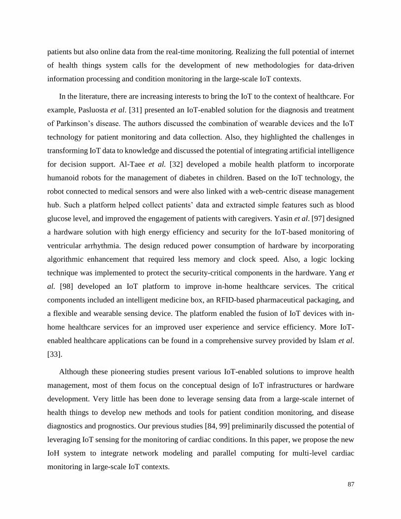
87
patients but also online data from the real-time monitoring. Realizing the full potential of internet
of health things system calls for the development of new methodologies for data-driven
information processing and condition monitoring in the large-scale IoT contexts.
In the literature, there are increasing interests to bring the IoT to the context of healthcare. For
example, Pasluosta et al. [31] presented an IoT-enabled solution for the diagnosis and treatment
of Parkinson’s disease. The authors discussed the combination of wearable devices and the IoT
technology for patient monitoring and data collection. Also, they highlighted the challenges in
transforming IoT data to knowledge and discussed the potential of integrating artificial intelligence
for decision support. Al-Taee et al. [32] developed a mobile health platform to incorporate
humanoid robots for the management of diabetes in children. Based on the IoT technology, the
robot connected to medical sensors and were also linked with a web-centric disease management
hub. Such a platform helped collect patients’ data and extracted simple features such as blood
glucose level, and improved the engagement of patients with caregivers. Yasin et al. [97] designed
a hardware solution with high energy efficiency and security for the IoT-based monitoring of
ventricular arrhythmia. The design reduced power consumption of hardware by incorporating
algorithmic enhancement that required less memory and clock speed. Also, a logic locking
technique was implemented to protect the security-critical components in the hardware. Yang et
al. [98] developed an IoT platform to improve in-home healthcare services. The critical
components included an intelligent medicine box, an RFID-based pharmaceutical packaging, and
a flexible and wearable sensing device. The platform enabled the fusion of IoT devices with in-
home healthcare services for an improved user experience and service efficiency. More IoT-
enabled healthcare applications can be found in a comprehensive survey provided by Islam et al.
[33].
Although these pioneering studies present various IoT-enabled solutions to improve health
management, most of them focus on the conceptual design of IoT infrastructures or hardware
development. Very little has been done to leverage sensing data from a large-scale internet of
health things to develop new methods and tools for patient condition monitoring, and disease
diagnostics and prognostics. Our previous studies [84, 99] preliminarily discussed the potential of
leveraging IoT sensing for the monitoring of cardiac conditions. In this paper, we propose the new
IoH system to integrate network modeling and parallel computing for multi-level cardiac
monitoring in large-scale IoT contexts.
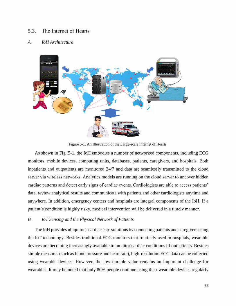
88
5.3. The Internet of Hearts
A. IoH Architecture
Figure 5-1. An Illustration of the Large-scale Internet of Hearts.
As shown in Fig. 5-1, the IoH embodies a number of networked components, including ECG
monitors, mobile devices, computing units, databases, patients, caregivers, and hospitals. Both
inpatients and outpatients are monitored 24/7 and data are seamlessly transmitted to the cloud
server via wireless networks. Analytics models are running on the cloud server to uncover hidden
cardiac patterns and detect early signs of cardiac events. Cardiologists are able to access patients’
data, review analytical results and communicate with patients and other cardiologists anytime and
anywhere. In addition, emergency centers and hospitals are integral components of the IoH. If a
patient’s condition is highly risky, medical intervention will be delivered in a timely manner.
B. IoT Sensing and the Physical Network of Patients
The IoH provides ubiquitous cardiac care solutions by connecting patients and caregivers using
the IoT technology. Besides traditional ECG monitors that routinely used in hospitals, wearable
devices are becoming increasingly available to monitor cardiac conditions of outpatients. Besides
simple measures (such as blood pressure and heart rate), high-resolution ECG data can be collected
using wearable devices. However, the low durable value remains an important challenge for
wearables. It may be noted that only 80% people continue using their wearable devices regularly
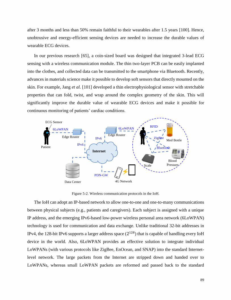
89
after 3 months and less than 50% remain faithful to their wearables after 1.5 years [100]. Hence,
unobtrusive and energy-efficient sensing devices are needed to increase the durable values of
wearable ECG devices.
In our previous research [65], a coin-sized board was designed that integrated 3-lead ECG
sensing with a wireless communication module. The thin two-layer PCB can be easily implanted
into the clothes, and collected data can be transmitted to the smartphone via Bluetooth. Recently,
advances in materials science make it possible to develop soft sensors that directly mounted on the
skin. For example, Jang et al. [101] developed a thin electrophysiological sensor with stretchable
properties that can fold, twist, and wrap around the complex geometry of the skin. This will
significantly improve the durable value of wearable ECG devices and make it possible for
continuous monitoring of patients’ cardiac conditions.
Figure 5-2. Wireless communication protocols in the IoH.
The IoH can adopt an IP-based network to allow one-to-one and one-to-many communications
between physical subjects (e.g., patients and caregivers). Each subject is assigned with a unique
IP address, and the emerging IPv6-based low-power wireless personal area network (6LoWPAN)
technology is used for communication and data exchange. Unlike traditional 32-bit addresses in
IPv4, the 128-bit IPv6 supports a larger address space (2128) that is capable of handling every IoH
device in the world. Also, 6LoWPAN provides an effective solution to integrate individual
LoWPANs (with various protocols like ZigBee, EnOcean, and SNAP) into the standard Internet-
level network. The large packets from the Internet are stripped down and handed over to
LoWPANs, whereas small LoWPAN packets are reformed and passed back to the standard
Edge Router
6LoWPAN
Patient
ECG Sensor
Data Center
Internet IPv6
Edge Router IPv6
6LoWPAN RFID
ZigBee
Bluetooth
Blood
Pressure Scale
Med Bottle
PDN-GW
4G Network
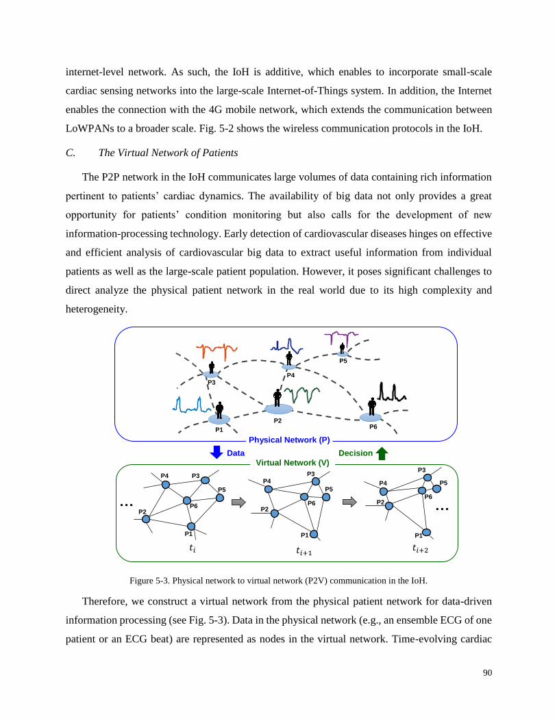
90
internet-level network. As such, the IoH is additive, which enables to incorporate small-scale
cardiac sensing networks into the large-scale Internet-of-Things system. In addition, the Internet
enables the connection with the 4G mobile network, which extends the communication between
LoWPANs to a broader scale. Fig. 5-2 shows the wireless communication protocols in the IoH.
C. The Virtual Network of Patients
The P2P network in the IoH communicates large volumes of data containing rich information
pertinent to patients’ cardiac dynamics. The availability of big data not only provides a great
opportunity for patients’ condition monitoring but also calls for the development of new
information-processing technology. Early detection of cardiovascular diseases hinges on effective
and efficient analysis of cardiovascular big data to extract useful information from individual
patients as well as the large-scale patient population. However, it poses significant challenges to
direct analyze the physical patient network in the real world due to its high complexity and
heterogeneity.
Figure 5-3. Physical network to virtual network (P2V) communication in the IoH.
Therefore, we construct a virtual network from the physical patient network for data-driven
information processing (see Fig. 5-3). Data in the physical network (e.g., an ensemble ECG of one
patient or an ECG beat) are represented as nodes in the virtual network. Time-evolving cardiac
P3
P1 P2
P4
P5
P6
P1
P5
P6
P3 P4
P2 P6
P5
P3
P4
P2
P1 P1
P2
P4
P3
P6
P5
𝑡𝑖 𝑡𝑖+1
Decision Data
Physical Network (P)
Virtual Network (V)
… …
𝑡𝑖+2
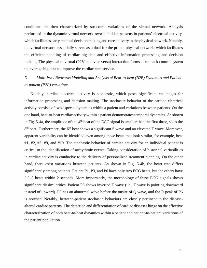
91
conditions are then characterized by structural variations of the virtual network. Analysis
performed in the dynamic virtual network reveals hidden patterns in patients’ electrical activity,
which facilitates early medical decision making and care delivery in the physical network. Notably,
the virtual network essentially serves as a dual for the primal physical network, which facilitates
the efficient handling of cardiac big data and effective information processing and decision
making. The physical to virtual (P2V, and vice versa) interaction forms a feedback control system
to leverage big data to improve the cardiac care service.
D. Multi-level Networks Modeling and Analysis of Beat-to-beat (B2B) Dynamics and Patient-
to-patient (P2P) variations.
Notably, cardiac electrical activity is stochastic, which poses significant challenges for
information processing and decision making. The stochastic behavior of the cardiac electrical
activity consists of two aspects: dynamics within a patient and variations between patients. On the
one hand, beat-to-beat cardiac activity within a patient demonstrates temporal dynamics. As shown
in Fig. 5-4a, the amplitude of the 4th beat of the ECG signal is smaller than the first three, so as the
8th beat. Furthermore, the 6th beat shows a significant S wave and an elevated T wave. Moreover,
apparent variability can be identified even among those beats that look similar, for example, beat
#1, #2, #3, #9, and #10. The stochastic behavior of cardiac activity for an individual patient is
critical to the identification of arrhythmic events. Taking consideration of historical variabilities
in cardiac activity is conducive to the delivery of personalized treatment planning. On the other
hand, there exist variations between patients. As shown in Fig. 5-4b, the heart rate differs
significantly among patients. Patient P1, P3, and P6 have only two ECG beats, but the others have
2.5–3 beats within 2 seconds. More importantly, the morphology of these ECG signals shows
significant dissimilarities. Patient P3 shows inverted T wave (i.e., T wave is pointing downward
instead of upward). P3 has an abnormal wave before the onsite of Q wave, and the R peak of P6
is notched. Notably, between-patient stochastic behaviors are closely pertinent to the disease-
altered cardiac patterns. The detection and differentiation of cardiac diseases hinge on the effective
characterization of both beat-to-beat dynamics within a patient and patient-to-patient variations of
the patient population.
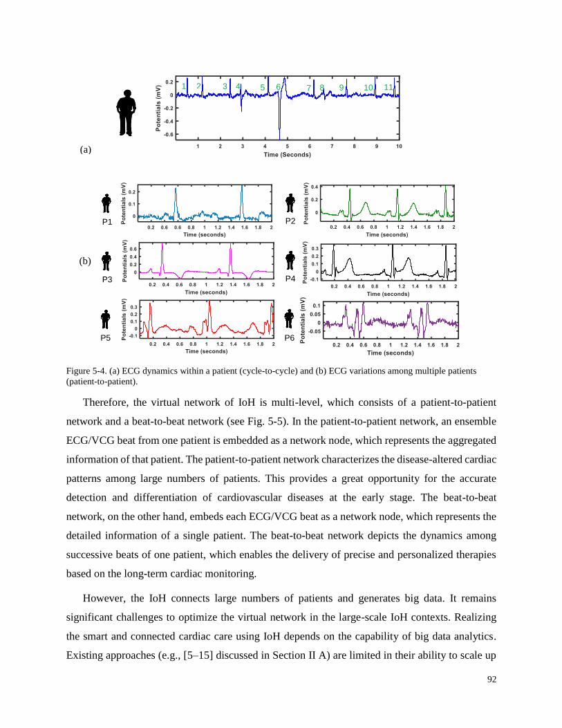
92
Figure 5-4. (a) ECG dynamics within a patient (cycle-to-cycle) and (b) ECG variations among multiple patients
(patient-to-patient).
Therefore, the virtual network of IoH is multi-level, which consists of a patient-to-patient
network and a beat-to-beat network (see Fig. 5-5). In the patient-to-patient network, an ensemble
ECG/VCG beat from one patient is embedded as a network node, which represents the aggregated
information of that patient. The patient-to-patient network characterizes the disease-altered cardiac
patterns among large numbers of patients. This provides a great opportunity for the accurate
detection and differentiation of cardiovascular diseases at the early stage. The beat-to-beat
network, on the other hand, embeds each ECG/VCG beat as a network node, which represents the
detailed information of a single patient. The beat-to-beat network depicts the dynamics among
successive beats of one patient, which enables the delivery of precise and personalized therapies
based on the long-term cardiac monitoring.
However, the IoH connects large numbers of patients and generates big data. It remains
significant challenges to optimize the virtual network in the large-scale IoH contexts. Realizing
the smart and connected cardiac care using IoH depends on the capability of big data analytics.
Existing approaches (e.g., [5–15] discussed in Section II A) are limited in their ability to scale up
(a)
(b)
1 2 3 4 5 6 7 8 9 10 11
P1 P2
P3 P4
P5 P6
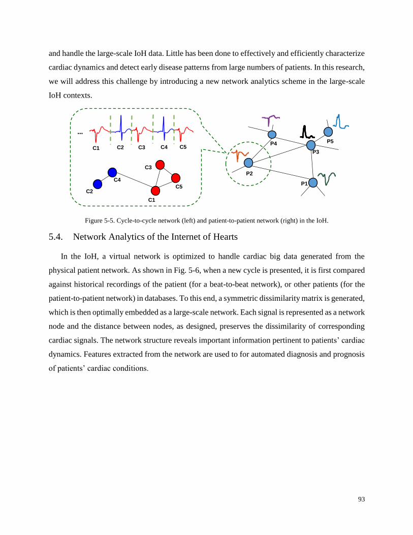
93
and handle the large-scale IoH data. Little has been done to effectively and efficiently characterize
cardiac dynamics and detect early disease patterns from large numbers of patients. In this research,
we will address this challenge by introducing a new network analytics scheme in the large-scale
IoH contexts.
Figure 5-5. Cycle-to-cycle network (left) and patient-to-patient network (right) in the IoH.
5.4. Network Analytics of the Internet of Hearts
In the IoH, a virtual network is optimized to handle cardiac big data generated from the
physical patient network. As shown in Fig. 5-6, when a new cycle is presented, it is first compared
against historical recordings of the patient (for a beat-to-beat network), or other patients (for the
patient-to-patient network) in databases. To this end, a symmetric dissimilarity matrix is generated,
which is then optimally embedded as a large-scale network. Each signal is represented as a network
node and the distance between nodes, as designed, preserves the dissimilarity of corresponding
cardiac signals. The network structure reveals important information pertinent to patients’ cardiac
dynamics. Features extracted from the network are used to for automated diagnosis and prognosis
of patients’ cardiac conditions.
P4
P2
P1
P3
P5 …
C1 C2 C3 C4 C5
C3
C1
C5 C4
C2
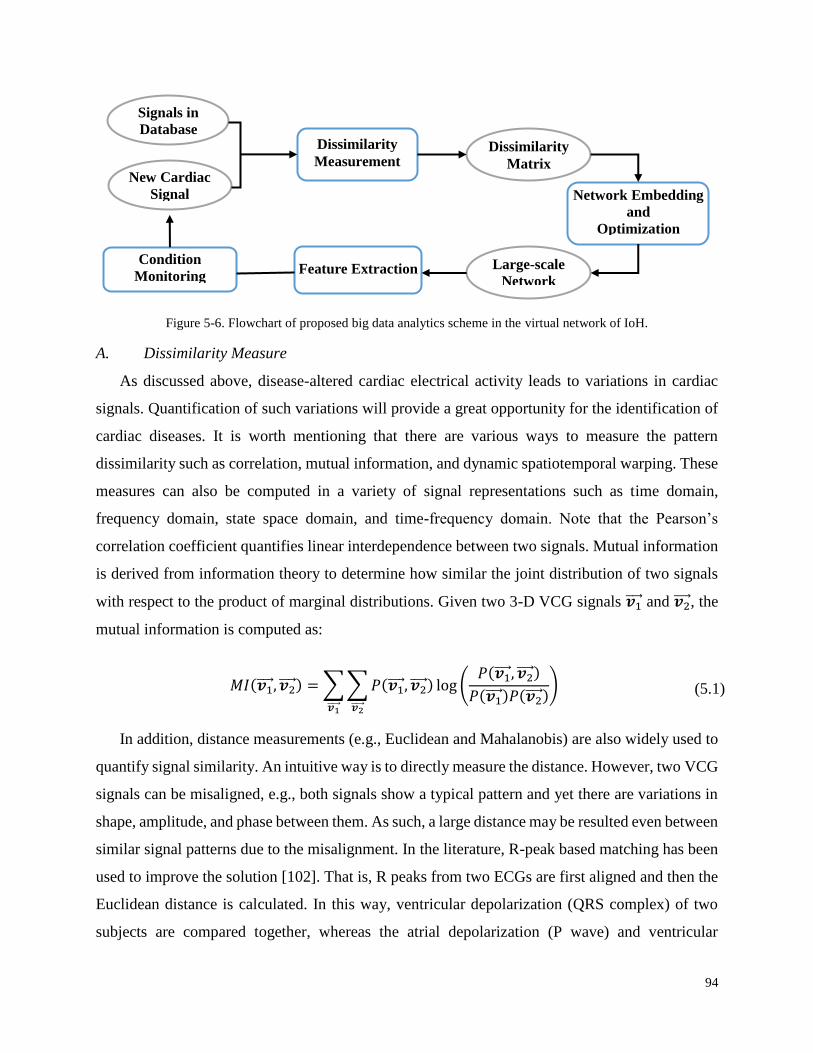
94
Figure 5-6. Flowchart of proposed big data analytics scheme in the virtual network of IoH.
A. Dissimilarity Measure
As discussed above, disease-altered cardiac electrical activity leads to variations in cardiac
signals. Quantification of such variations will provide a great opportunity for the identification of
cardiac diseases. It is worth mentioning that there are various ways to measure the pattern
dissimilarity such as correlation, mutual information, and dynamic spatiotemporal warping. These
measures can also be computed in a variety of signal representations such as time domain,
frequency domain, state space domain, and time-frequency domain. Note that the Pearson’s
correlation coefficient quantifies linear interdependence between two signals. Mutual information
is derived from information theory to determine how similar the joint distribution of two signals
with respect to the product of marginal distributions. Given two 3-D VCG signals 𝒗1⃗⃗⃗⃗ and 𝒗2⃗⃗⃗⃗ , the
mutual information is computed as:
𝑀𝐼(𝒗1⃗⃗⃗⃗ , 𝒗2⃗⃗⃗⃗ ) = ∑∑𝑃(𝒗1⃗⃗⃗⃗ , 𝒗2⃗⃗⃗⃗ )
𝒗2⃗⃗ ⃗⃗ 𝒗1⃗⃗ ⃗⃗
log (𝑃(𝒗1⃗⃗⃗⃗ , 𝒗2⃗⃗⃗⃗ )
𝑃(𝒗1⃗⃗⃗⃗ )𝑃(𝒗2⃗⃗⃗⃗ )) (5.1)
In addition, distance measurements (e.g., Euclidean and Mahalanobis) are also widely used to
quantify signal similarity. An intuitive way is to directly measure the distance. However, two VCG
signals can be misaligned, e.g., both signals show a typical pattern and yet there are variations in
shape, amplitude, and phase between them. As such, a large distance may be resulted even between
similar signal patterns due to the misalignment. In the literature, R-peak based matching has been
used to improve the solution [102]. That is, R peaks from two ECGs are first aligned and then the
Euclidean distance is calculated. In this way, ventricular depolarization (QRS complex) of two
subjects are compared together, whereas the atrial depolarization (P wave) and ventricular
New Cardiac
Signal
Dissimilarity
Measurement Dissimilarity
Matrix
Network Embedding
and
Optimization
Feature Extraction Large-scale
Network
Condition
Monitoring
Signals in
Database
95
repolarization (T wave) may still be misaligned. Thus, there is a need to optimally align two ECG
signals to compare the electrical activity of corresponding heart chambers.
Dynamic warping is a well-known approach to nonlinearly warp two signals for optimal
alignment [40]. In our previous study [81], we extended time domain warping into spatiotemporal
warping to address misalignment between multi-lead ECG signals. For example, given two VCG
signals 𝒗1⃗⃗⃗⃗ and 𝒗2⃗⃗⃗⃗ , with length 𝑉1 and 𝑉2, respectively. The spatiotemporal warping can be defined
as: min𝑊
[∑ ‖𝒗𝟏⃗⃗⃗⃗ (𝑡𝑖) − 𝒗𝟐⃗⃗⃗⃗ (𝑡𝑗)‖(𝑡𝑖,𝑡𝑗)∈𝑊 ], where 𝑊 is the warping path. 𝑡𝑖 is an index selected from
𝒗1⃗⃗⃗⃗ and 𝑡𝑗 is from 𝒗2⃗⃗⃗⃗ . To find the warping path, a distance matrix 𝐷 is computed with each element
𝐷(𝑖, 𝑗) = ‖𝒗1⃗⃗⃗⃗ (𝑖) − 𝒗2⃗⃗⃗⃗ (𝑗)‖, 𝑖 = 1,2, … , 𝑉1 and 𝑗 = 1,2, … , 𝑉2. The warping path 𝑊 connects
𝐷(1,1) and 𝐷(𝑉1,𝑉2), and recursively computed using dynamic programming approach:
𝐺(𝑖, 𝑗) = 𝐷(𝑖, 𝑗) + min {
𝐺(𝑖, 𝑗– 1)𝐺(𝑖 − 1, 𝑗 − 1)
𝐺(𝑖 − 1, 𝑗) (5.2)
The spatiotemporal dissimilarity between two multidimensional signals 𝒗1⃗⃗⃗⃗ and 𝒗2⃗⃗⃗⃗ (i.e., the
warping distance) can then be calculated as: 𝛿𝒗1⃗⃗ ⃗⃗ ,𝒗2⃗⃗ ⃗⃗ =𝐺(𝑉1,𝑉2)
𝑉1+𝑉2. In this way, dynamic warping
optimally aligns two signals to ensure a fair comparison. In other words, atrial depolarization (P
wave), ventricular depolarization (QRS complex) and repolarization (T wave) from one beat is
compared with the corresponding one from the other beat, as opposed to the incorrect comparison
between atrial and ventricular patterns that generates misleading results.
B. Data-driven Modeling and Optimization of a Large-scale Dynamic Network
Dynamic warping between 𝑁 VCG signals generates a 𝑁 × 𝑁 warping matrix ∆, with each
element 𝛿𝑖𝑗 characterizes the spatiotemporal dissimilarity between VCGs 𝒗𝑖⃗⃗ ⃗ and 𝒗𝑗⃗⃗ ⃗ . However,
the warping matrix itself is difficult to be used as features for the identification of disease properties
in predictive modeling and monitoring. In addition, the measure of Euclidean distance is not
directional and can mix the distances that are equal in magnitudes but along different spatial
directions [81]. There is a need to transfer the warping matrix into feature vectors that not only
preserve the warping matrix but also recover directional differences among space-time signals.
One way to realize such transformation is network embedding, which represents the signals as
network nodes in a high-dimensional space. The Euclidean distance between each pair of nodes
96
preserves the warping distance of corresponding space-time signals. A commonly used network
embedding approach is classic multidimensional scaling (MDS). Let 𝒙𝑖 and 𝒙𝑗 denote the location
of 𝑖𝑡ℎ and 𝑗𝑡ℎ nodes in the network and 𝛿𝑖𝑗 is the dissimilarity between 𝑖𝑡ℎ and 𝑗𝑡ℎ cardiac signals
in the warping matrix ∆. Then, the cost function of network embedding can be formulated as:
𝑓 = ∑(‖𝒙𝑖 − 𝒙𝑗‖ − 𝛿𝑖𝑗)2
𝑖,𝑗
(5.3)
To optimize the location of network nodes, a Gram matrix B is reconstructed from dissimilarity
matrix ∆ as B = −1
2𝐻∆(2)𝐻, where H = 𝐼 − 𝑁−1𝟏𝟏𝑇 is a centering matrix. The element 𝑏𝑖𝑗 in
matrix B is obtained as:
𝑏𝑖𝑗 = −1
2[𝛿𝑖𝑗
2 −1
𝑁∑ 𝛿𝑖𝑘
2
𝑁
𝑘=1
−1
𝑁∑ 𝛿𝑘𝑗
2
𝑁
𝑘=1
+1
𝑁2∑ ∑ 𝛿𝑔ℎ
2
𝑁
ℎ=1
𝑁
𝑔=1
] (5.4)
The Gram matrix B can be defined as the scalar product 𝐵 = 𝑋𝑋𝑇, which is further written as B =
𝑉𝛬𝑉𝑇 = 𝑉√𝛬√𝛬𝑉𝑇 by eigen-decomposition. Here, 𝑉 is a matrix of eigenvectors and 𝛬 is a
diagonal matrix of eigenvalues. Hence, optimal coordinates of network nodes are obtained as: 𝑋 =
𝑉√𝛬.
In the past decade, stochastic learning approaches have been increasingly adopted in analytics
methods to solve optimization problems that involve big data. Notably, big data poses two
significant challenges for optimization. On one hand, the dimensionality of the data is high. As
such, second-order optimization is sometimes prohibitive. Thus, first order methods are preferred,
e.g., gradient-based method. On the other hand, large volumes of data make it impractical for
algorithms to go through the entire dataset many times. Hence, a stochastic approach is more suited
to handle big data, because only one data sample is considered at every iteration. Moreover, it has
been shown that the convergence of stochastic approaches for the optimization of convex and
concave functions is guaranteed in most cases.
Motivated by [85], we rewrite the cost function of Eq. (5.3) as:
97
𝑓 =1
2∑∑(‖𝒙𝑖
𝑡 − 𝒙𝑗𝑡‖ − 𝛿𝑖𝑗)
2
𝑗≠𝑖𝑖
𝛹(‖𝒙𝑖𝑡 − 𝒙𝑗
𝑡‖, 𝜆) (5.5)
where 𝛹(∙) is a bounded and monotonically decreasing function to favor the local topology in the
network and 𝜆 is defines the neighborhood radius. One example of 𝛹(∙) is a step function:
𝛹(‖𝒙𝑖𝑡 − 𝒙𝑗
𝑡‖, 𝜆) = {1 if ‖𝒙𝑖
𝑡 − 𝒙𝑗𝑡‖ ≤ 𝜆
0 if ‖𝒙𝑖𝑡 − 𝒙𝑗
𝑡‖ > 𝜆 (5.6)
Minimization of Eq. (5.5) with respect to 𝒙𝑗’s achieves the optimal location of the network nodes.
Notably, the decrease in the value of 𝐹 can be considered as a summation of partial decrease
resulted from each network node 𝑖, i.e., 𝑓 =1
2∑ 𝑓𝑖𝑖 . The optimization of Eq. (5.5) works as follows
[85]: in each iteration, a node 𝑖 is randomly selected and its location (e.g., 𝒙𝑖) is fixed. Then, all
other nodes 𝒙𝑗(𝑗 ≠ 𝑖) are updated based on the following rule:
𝒙𝑗𝑡+1 = 𝒙𝑗
𝑡 − 𝜂𝑡
𝜕𝑓𝑖𝜕𝒙𝑗
𝑡 (5.7)
where the learning rate 𝜂𝑡 is a monotonically deceasing function. Different forms of 𝜂𝑡 can be
used to decay the learning rate along the learning process and we adopt an exponential
function: 𝜂𝑡 = 𝜂0 (𝜂𝑇
𝜂0)𝑡
, where constants 𝜂0 and 𝜂𝑇 specify the initial and final scales of the
learning rate and the ratio of 𝜂𝑇 and 𝜂0determines the decaying speed.
In the update rule of Eq. (5.7), one node is pinned and all 𝑁 − 1 nodes need to be updated at
each iteration. This is different from conventional stochastic optimization rules, which update only
one subject at each iteration. Advantages of updating 𝑁 − 1 nodes include 1) easy to escape from
local minimum, 2) robust to initial node layout, and 3) fast convergence rate. However, this may
introduce a larger variation compared with conventional update. Here, the update of 𝒙𝑗 only
depends on its relationship (i.e., the gradient) with respect to the pinned node 𝒙𝑖. On the contrary,
the update of 𝒙𝑗 is controlled by its relationship with all other nodes in the conventional rule. As
such, the convergence of the update rule of Eq. (5.7) can be influenced by the selection of model
parameters (e.g., 𝜂𝑡) and requires fine tunes of these parameters, which makes it not practical in

98
the clinical practice. Therefore, a new cost function is introduced to regularize the update of 𝒙𝑗
as:
𝑓 =1
2[∑∑(‖𝒙𝑖
𝑡 − 𝒙𝑗𝑡‖ − 𝛿𝑖𝑗)
2
𝑗≠𝑖𝑖
+ 𝜗𝑡‖𝒙𝑗𝑡 − 𝒙𝑗
𝑡−1‖2
2]𝛹(‖𝒙𝑖
𝑡 − 𝒙𝑗𝑡‖, 𝜆) (5.8)
where the second term 𝜗𝑡‖𝒙𝑗𝑡 − 𝒙𝑗
𝑡−1‖2
2 regularizes the update of 𝒙𝑗 between successive iterations.
Notably, the new cost function contains both spaital regularization term (𝑓𝑆 = ∑ ∑ (‖𝒙𝑖𝑡 −𝑗≠𝑖𝑖
𝒙𝑗𝑡‖ − 𝛿𝑖𝑗)
2) and temporal regularization term (𝑓𝑇 = 𝜗𝑡‖𝒙𝑗
𝑡 − 𝒙𝑗𝑡−1‖
2
2). The update rule of
stochastic network embedding is then given as:
{𝒙𝑗
𝑡+1 = 𝒙𝑗𝑡 − 𝜂𝑡 (∇𝑓𝑠 + 𝜗𝑡(𝒙𝑗
𝑡 − 𝒙𝑗𝑡−1)) if ‖𝒙𝑖
𝑡 − 𝒙𝑗𝑡‖ ≤ 𝜆𝑡
𝒙𝑗𝑡+1 = 𝒙𝑗
𝑡 if ‖𝒙𝑖𝑡 − 𝒙𝑗
𝑡‖ > 𝜆𝑡
(5.9)
where ∇𝑓𝑠 =‖𝒙𝑖
𝑡−𝒙𝑗𝑡‖−𝛿𝑖𝑗
‖𝒙𝑖𝑡−𝒙𝑗
𝑡‖ (𝒙𝑗
𝑡 − 𝒙𝑖𝑡). This approach iterates until the maximum number of learning
epoch is reached. The stochastic embedding approach is summarized in Algorithm 5-1.
Algorithm 5-1 Stochastic network embedding – serial computing
Input: dissimilarity matrix ∆ (𝛿𝑖𝑗)
Output: coordinates of nodes 𝒙𝑖, 𝑖 ∈ {1, 2, … ,𝑁} in the high-dimensional network
1: 𝑇 – number of epoch
2: initialize 𝒙𝑖, learning rate {𝜂𝑡}𝑡=1𝑇 ,neighborhood radius {𝜆𝑡}𝑡=1
𝑇 , and regularization
parameter {𝜗𝑡}𝑡=1𝑇
3: for 𝑡 =1, 2, …, 𝑇 do
4: create index sequence 𝜘 by random permutation of {1, 2, … ,𝑁}
5: for 𝑛 = 1 to 𝑁 do
6: randomly draw 𝑖 ∈ 𝜘 , Fix the 𝒙𝑖𝑡
7: update using Eq. (5.9)
8: end for
9: end for
Compared with MDS, the computational complexity of Algorithm 5-1 is reduced (i.e., 𝑂(𝑁)
instead of 𝑂(𝑁2)). However, it is still expensive when large numbers of nodes are involved in the
network. Thus, it is imperative to parallelize the algorithm and utilize more computing resources
collaboratively. However, the inherently sequential nature of Algorithm 5-1 poses significant
challenges for parallelization. An algorithm can be parallelized if the computing task can be

99
divided and results from individual processors (or computers) are independent of each other.
Notably, fixing the location of nodes 𝑎 or 𝑏 and updating the location of other nodes will result in
different locations of 𝑐 especially when 𝑎 and 𝑏 are far from each other. Thus, Algorithm 5-1 is
difficult to be parallelized.
To address this challenge, we combine stochastic embedding with batch learning, which results
in the mini-batch stochastic embedding. Instead of considering one sample at a time, the mini-
batch algorithm considers multiple samples (i.e., a mini-batch) simultaneously at each iteration
[86]. Assume the total number of data 𝑁 can be partitioned into 𝑀 mini-batches, each of the size
𝑚. Given a randomly selected mini-batch 𝛾, the objective function on the mini-batch can be written
as 𝑓𝛾 =1
|𝛾|∑ 𝑓𝑖𝑖∈𝛾 , where |𝛾| is the size of a batch. At each iteration, the mini-batch stochastic
embedding accumulates sub-gradients with respect to |𝛾| samples in the batch and calculate the
average gradients as:
∇𝑓𝛾(𝒙𝑗𝑡) =
1
|𝛾|∑∇𝑓𝑖(𝒙𝑗
𝑡)
𝑖∈𝛾
(5.10)
where ∇𝑓𝑖(𝒙𝑗𝑡) =
𝜕𝑓𝑖
𝜕𝒙𝑗𝑡. As such, each mini-batch generates a single average gradient. At the end of
each batch, mini-batch stochastic embedding feeds ∇𝑓𝛾(𝒙𝑗𝑡) to update the location of all other
nodes 𝒙𝑗𝑡 (𝑗 ≠ 𝑖) as:
𝒙𝑗𝑡 = 𝒙𝑗
𝑡 − 𝜂𝑡∇𝑓𝛾(𝒙𝑗𝑡) (5.11)
As the update rule is used less frequently, the mini-batch stochastic embedding provides
computational benefits.
More importantly, each mini-batch 𝛾 can be further considered as a combination of multiple
subsets, i.e., 𝛾 = 𝛾1 ∪ 𝛾2 ∪,… ,∪ 𝛾𝑆. Thus, the calculation of sub-gradients in Eq. (5.10) can be
represented as:

100
∇𝑓𝛾(𝒙𝑗𝑡) =
1
|𝛾|∑∇𝑓𝑖(𝒙𝑗
𝑡)
𝑖∈𝛾
=1
|𝛾|[∑ ∇𝑓𝑖(
𝑖∈𝛾1
𝒙𝑗𝑡) + ∑ ∇𝑓𝑖(
𝑖∈𝛾2
𝒙𝑗𝑡) + ⋯+ ∑ ∇𝑓𝑖(
𝑖∈𝛾𝑆
𝒙𝑗𝑡)]
(5.12)
To this end, the mini-batch stochastic embedding can be readily implemented in a parallel manner.
That is, the mini- batch 𝛾 can be divided and the computation of average gradient can be assigned
to 𝑆 individual processors. Each processor s will compute ∑ ∇𝑓𝑖(𝑖∈𝛾𝑠𝒙𝑗
𝑡) and results from 𝑆
processors are combined using Eq. (5.12) to return the average gradient with respect to all samples
in the mini-batch. The parallelized stochastic network embedding algorithm is summarized in
Algorithm 5-2.
Algorithm 5-2 Stochastic network embedding – parallel computing
1: initialize as Algorithm 5-1 step 1 and 2
2: randomly partition data into 𝑀 mini-batches 𝛾1, 𝛾2, …, 𝛾𝑀
3: start parallel pool with 𝑆 processors
4: for 𝑡 =1, 2, …, 𝑇 do
5: randomly choose a mini-batch 𝛾𝑡
6: partition 𝛾𝑡 into subsets 𝛾𝑡,1, 𝛾𝑡,2,…, 𝛾𝑡,𝑆, each with size 𝑚
7: for 𝑛 = 1 to 𝑀 do {in parallel}
8: processor n gets partition 𝛾𝑡,𝑛
9: solve the sub-problem ∇𝑓𝑖∈𝛾𝑡,𝑛(𝒙𝑗
𝑡) on 𝛾𝑡,𝑛 by Algorithm 5-1
10: end for
11: average over the batch size 𝑚 and update 𝒙𝑗𝑡
12: end for
13: close parallel pool
C. Network-based Monitoring of Cardiac Processes
To this end, cardiovascular big data generated from the physical patient network are handled
by the virtual IoH network. Coordinates of each node in the virtual network are optimized to
represent the cardiac condition of the corresponding patient. Patients with similar conditions are
located closely, thereby forming multiple communities in the network. Distances among nodes
with the same community are small, whereas large distances exist among different groups.
Network features (such as coordinates of nodes and community structures) can then be extracted
for the diagnosis and prognosis of cardiovascular diseases.
101
In the literature, various predictive modeling approaches are available to quantitatively
associate network features to patients’ cardiac conditions. For example, k-nearest neighbors,
logistic regression, and neural networks. Practitioners can select the most suitable approach based
on the complexity of data and requirements of processing speed. In this study, we introduce another
domain of methods, namely, statistical control charts. The most widely used control chart is the
Shewhart chart. Two types of Shewhart charts, i.e., X-bar chart and R-chart, are constructed to
monitor the mean and variance of process data in both manufacturing and healthcare. With the
advancement of sensing technology, complex and higher dimensional process data are obtained.
To address the data complexity, multivariate control charts were more and more used in the process
control. The most widely used multivariate chart is the Hotelling 𝑇2 chart, which is an extension
of Shewhart chart for the monitoring of the mean vector of the process. The 𝑇2 statistic for the 𝑖th
patient is computed as:
𝑇2(𝑖) = (𝒙𝑖 − �̅�)𝑇 𝑺−1(𝒙𝑖 − �̅�) (5.13)
Here, �̅� is an averaged location of network nodes and 𝑺 is the covariance matrix. However, 𝑺 can
be singular when the dimensionality of node coordinate 𝒙 is high. Therefore, we computed the 𝑇2
statistic in Eq. (5.14) using the set of principal components as in our previous study [103]:
𝑇2(𝑖) = (𝒙𝑖 − �̅�)𝑇 𝑺−1(𝒙𝑖 − 𝒙) = ∑𝐙(𝑖, 𝑟)2
𝜆𝑟2
𝑄
𝑟=1
(5.14)
The upper control limit (UCL) of Hotelling 𝑇2control chart is estimated as:
𝑈𝐶𝐿𝑇2 = 𝑞(𝑁 + 1)(𝑁 − 1)
𝑁2 − 𝑁𝑞𝐹𝛼,𝑞,𝑀−𝑞 (5.15)
where 𝑞 is the dimensionality of 𝒙𝑖. 𝐹𝛼,𝑞,𝑀−𝑞 is the upper 100𝛼% of critical point of F distribution
with 𝑞 and 𝑁 − 𝑞 degree of freedoms. The significance level 𝛼 is set as 0.05.
5.5. Materials and Experimental Design
In this investigation, we evaluate and validate the developed methodology using both
simulation studies and real-world applications. As shown in Fig. 5-7, we evaluate four factor
groups in the simulation study as follows:

102
1) ECG segment: Different types of cardiovascular diseases will impact the morphology of
different ECG segments. For example, pulmonary hypertension will result in the right atrial
enlargement, which is reflected as enlarged P waves. Also, diseases occur in ventricles (e.g.,
myocardial infarctions) will impact the activity of ventricular depolarization and
repolarization, which lead to abnormal morphologies in QRS and T waves, respectively.
Notably, the length of QRS is the smallest, whereas P and T waves are larger. Segments with
smaller lengths pose greater challenges for the detection. It is important to test the proposed
algorithm on shifted ECG segments with different lengths.
2) Mean shift magnitude within an ECG segment: Disease-altered ECG morphology also reveals
the severity of the disease. When the disease is in the early stage, the morphology of an ECG
segment is changed slightly from the normal one. However, the shift magnitude is large when
the disease lasts for a long time. Notably, small shift magnitudes pose greater challenges for
the automated detection. It is important to implement the proposed algorithm on varying shift
magnitudes of ECG segments to evaluate the ability of early disease pattern recognition.
3) Dissimilarity measure: Effective measurement of the dissimilarity among ECG signals is a
prerequisite for achieving high detection power. The signal dissimilarity can be characterized
from various perspective, including morphological dissimilarity, signal correlation, and the
mutual dependence of the amount of information held in both signals. It is important to evaluate
the effectiveness of different measures and identify the most suitable one for a particular type
of disease.
4) Statistical control chart: Early diagnosis of cardiac diseases calls for not only the accurate
measure of signal dissimilarities but also effective detection and prediction tools. It is
important to evaluate various monitoring schemes under different scenarios (e.g., length of
shifted ECG segments and shift magnitudes) to identify the one that most sensitive to small
and early-stage abnormalities in the ECG signals.
In real-world applications, a continuously recorded ECG signals from the PhysioNet Long-term
ST database [104, 105] are used to evaluate the performance of the developed methodology. In the
database, signals were digitized at 250 Hz sampling rate with a 12-bit resolution over a range of
±10 mV. Beat-by-beat annotations are also provided, which labels each beat to be normal or a
certain type of disease. Two types of beats are identified in the continuous ECG records: beats
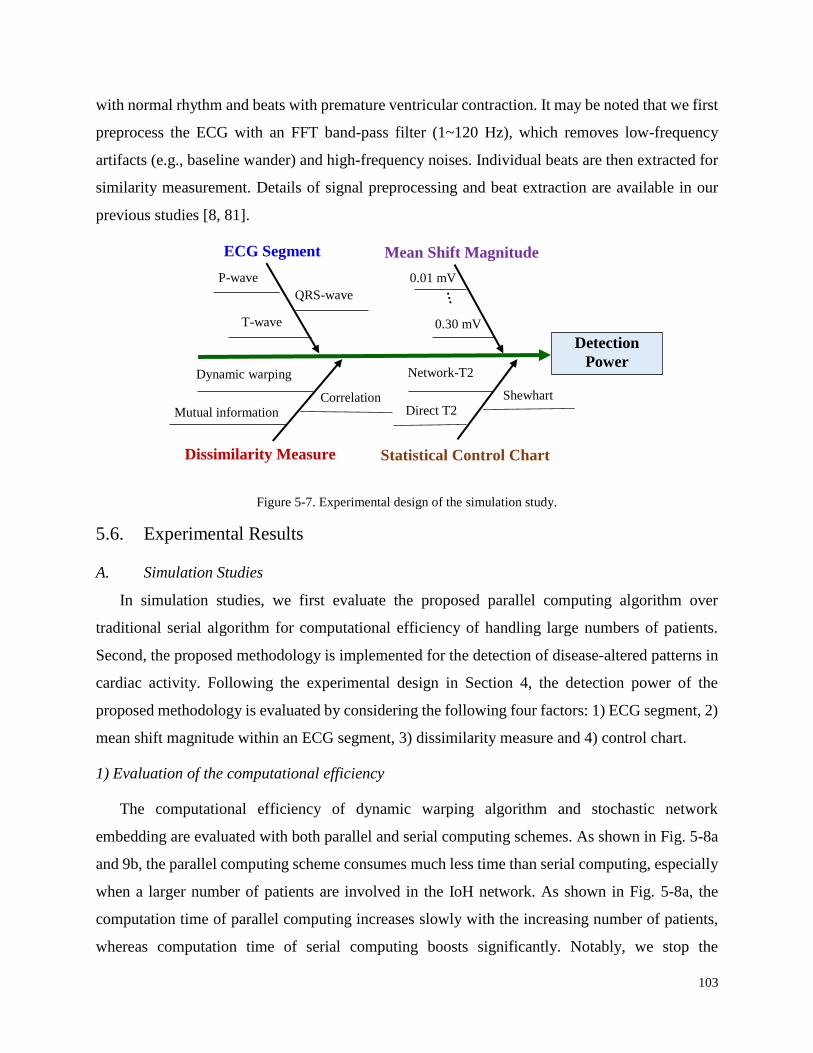
103
with normal rhythm and beats with premature ventricular contraction. It may be noted that we first
preprocess the ECG with an FFT band-pass filter (1~120 Hz), which removes low-frequency
artifacts (e.g., baseline wander) and high-frequency noises. Individual beats are then extracted for
similarity measurement. Details of signal preprocessing and beat extraction are available in our
previous studies [8, 81].
Figure 5-7. Experimental design of the simulation study.
5.6. Experimental Results
A. Simulation Studies
In simulation studies, we first evaluate the proposed parallel computing algorithm over
traditional serial algorithm for computational efficiency of handling large numbers of patients.
Second, the proposed methodology is implemented for the detection of disease-altered patterns in
cardiac activity. Following the experimental design in Section 4, the detection power of the
proposed methodology is evaluated by considering the following four factors: 1) ECG segment, 2)
mean shift magnitude within an ECG segment, 3) dissimilarity measure and 4) control chart.
1) Evaluation of the computational efficiency
The computational efficiency of dynamic warping algorithm and stochastic network
embedding are evaluated with both parallel and serial computing schemes. As shown in Fig. 5-8a
and 9b, the parallel computing scheme consumes much less time than serial computing, especially
when a larger number of patients are involved in the IoH network. As shown in Fig. 5-8a, the
computation time of parallel computing increases slowly with the increasing number of patients,
whereas computation time of serial computing boosts significantly. Notably, we stop the
Detection
Power
ECG Segment
Statistical Control Chart
Mean Shift Magnitude
P-wave QRS-wave
Dissimilarity Measure
T-wave
0.01 mV
0.30 mV
Dynamic warping
Mutual information Correlation
Network-T2
Shewhart Direct T2
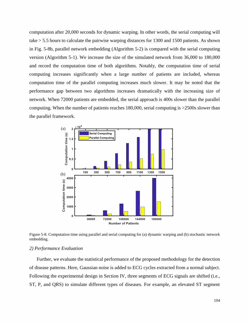
104
computation after 20,000 seconds for dynamic warping. In other words, the serial computing will
take > 5.5 hours to calculate the pairwise warping distances for 1300 and 1500 patients. As shown
in Fig. 5-8b, parallel network embedding (Algorithm 5-2) is compared with the serial computing
version (Algorithm 5-1). We increase the size of the simulated network from 36,000 to 180,000
and record the computation time of both algorithms. Notably, the computation time of serial
computing increases significantly when a large number of patients are included, whereas
computation time of the parallel computing increases much slower. It may be noted that the
performance gap between two algorithms increases dramatically with the increasing size of
network. When 72000 patients are embedded, the serial approach is 400s slower than the parallel
computing. When the number of patients reaches 180,000, serial computing is >2500s slower than
the parallel framework.
Figure 5-8. Computation time using parallel and serial computing for (a) dynamic warping and (b) stochastic network
embedding.
2) Performance Evaluation
Further, we evaluate the statistical performance of the proposed methodology for the detection
of disease patterns. Here, Gaussian noise is added to ECG cycles extracted from a normal subject.
Following the experimental design in Section IV, three segments of ECG signals are shifted (i.e.,
ST, P, and QRS) to simulate different types of diseases. For example, an elevated ST segment
(a)
(b)

105
corresponds to acute myocardial infarction. Also, a larger P wave indicates the potential atrial
enlargement. When the patient is associated with massive pericardial effusion, the voltage of QRS
will be lower, which is shown as a reduced QRS complex in the ECG signals. The severity of
disease can be represented by the shift magnitude of cardiac signals. In other words, a tiny shift
indicates the disease is in the early stage, whereas a large shift is associated with well-developed
disease conditions and calls for immediate medical intervention. Notably, ST is the longest
segment in the ECG signal. The P segment is shorter and QRS is with the smallest length.
In this study, we construct statistical control charts for the monitoring of patients’ cardiac
conditions. Similar to the SPC monitoring system of Zhou, Sun and Shi [9], three types of control
charts are constructed, including 1) a 𝑇2chart based on the network features (i.e., coordinates of
embedded network nodes), 2) a 𝑇2chart directly using the original ECG signals, and 3) a Shewhart
chart monitoring the mean change of the ECG signals. In total, 150 new ECG cycles are generated.
The first 50 cycles are considered as normal (i.e., in-control) signals, whereas mean shifts with
different magnitudes are added to the rest 100 cycles to generate disease-altered (i.e., out-of-
control) signals. The detection power is calculated as the number of out-of-control signals over
100. Notably, dissimilarities among ECG signals are measured by the spatiotemporal warping
approach.
As shown in Fig. 5-9, the network 𝑇2chart performs better than the Shewhart chart and the
𝑇2chart of original signals under all three scenarios. Specifically, the detection power of the
network 𝑇2 chart (blue triangles) quickly reaches one at very small shift magnitude (0.03 mV)
when the length of shifted segment is larger (shifted ST segments in Fig. 5-9a). When shifted
segments are shorter, network 𝑇2 chart is also sensitive to small disease-induced changes and the
detection power reaches one at the shift magnitude of 0.08 mV and 0.12 mV for P (Fig. 5-9b) and
QRS segments (Fig. 5-9c), respectively. The detection power of the 𝑇2chart of original signals
(orange squares) increases slower with the increase of shift magnitude compared with the network
𝑇2chart. When the length of shifted segment is short (shifted QRS segments in Fig. 5-9c), the
detection power is only 0.4 when the mean shift magnitude is 0.15 mV and it reaches one when
the shift magnitude is over 0.22 mV. Notably, the detection power of Shewhart chart is comparable
to the 𝑇2chart of original signals when the shift magnitude is large (e.g., ST segments in Fig. 5-
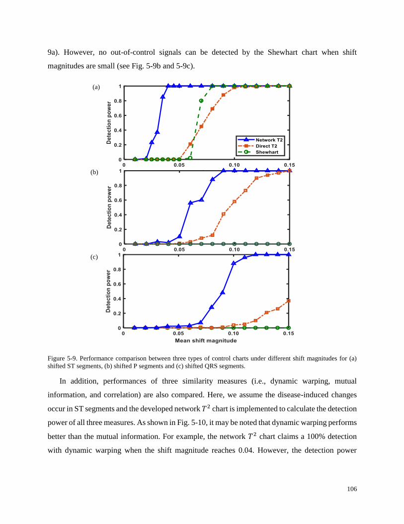
106
9a). However, no out-of-control signals can be detected by the Shewhart chart when shift
magnitudes are small (see Fig. 5-9b and 5-9c).
Figure 5-9. Performance comparison between three types of control charts under different shift magnitudes for (a)
shifted ST segments, (b) shifted P segments and (c) shifted QRS segments.
In addition, performances of three similarity measures (i.e., dynamic warping, mutual
information, and correlation) are also compared. Here, we assume the disease-induced changes
occur in ST segments and the developed network 𝑇2 chart is implemented to calculate the detection
power of all three measures. As shown in Fig. 5-10, it may be noted that dynamic warping performs
better than the mutual information. For example, the network 𝑇2 chart claims a 100% detection
with dynamic warping when the shift magnitude reaches 0.04. However, the detection power
(a)
(b)
(c)
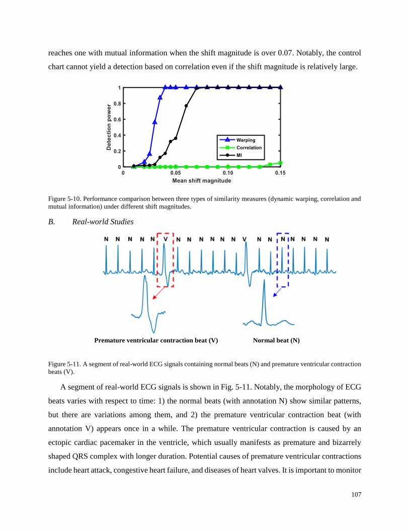
107
reaches one with mutual information when the shift magnitude is over 0.07. Notably, the control
chart cannot yield a detection based on correlation even if the shift magnitude is relatively large.
Figure 5-10. Performance comparison between three types of similarity measures (dynamic warping, correlation and
mutual information) under different shift magnitudes.
B. Real-world Studies
Figure 5-11. A segment of real-world ECG signals containing normal beats (N) and premature ventricular contraction
beats (V).
A segment of real-world ECG signals is shown in Fig. 5-11. Notably, the morphology of ECG
beats varies with respect to time: 1) the normal beats (with annotation N) show similar patterns,
but there are variations among them, and 2) the premature ventricular contraction beat (with
annotation V) appears once in a while. The premature ventricular contraction is caused by an
ectopic cardiac pacemaker in the ventricle, which usually manifests as premature and bizarrely
shaped QRS complex with longer duration. Potential causes of premature ventricular contractions
include heart attack, congestive heart failure, and diseases of heart valves. It is important to monitor
Premature ventricular contraction beat (V) Normal beat (N)
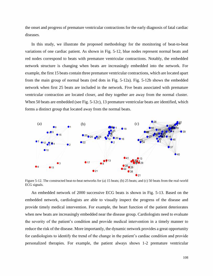
108
the onset and progress of premature ventricular contractions for the early diagnosis of fatal cardiac
diseases.
In this study, we illustrate the proposed methodology for the monitoring of beat-to-beat
variations of one cardiac patient. As shown in Fig. 5-12, blue nodes represent normal beats and
red nodes correspond to beats with premature ventricular contractions. Notably, the embedded
network structure is changing when beats are increasingly embedded into the network. For
example, the first 15 beats contain three premature ventricular contractions, which are located apart
from the main group of normal beats (red dots in Fig. 5-12a). Fig. 5-12b shows the embedded
network when first 25 beats are included in the network. Five beats associated with premature
ventricular contraction are located closer, and they together are away from the normal cluster.
When 50 beats are embedded (see Fig. 5-12c), 13 premature ventricular beats are identified, which
forms a distinct group that located away from the normal beats.
Figure 5-12. The constructed beat-to-beat networks for (a) 15 beats; (b) 25 beats; and (c) 50 beats from the real-world
ECG signals.
An embedded network of 2000 successive ECG beats is shown in Fig. 5-13. Based on the
embedded network, cardiologists are able to visually inspect the progress of the disease and
provide timely medical intervention. For example, the heart function of the patient deteriorates
when new beats are increasingly embedded near the disease group. Cardiologists need to evaluate
the severity of the patient’s condition and provide medical intervention in a timely manner to
reduce the risk of the disease. More importantly, the dynamic network provides a great opportunity
for cardiologists to identify the trend of the change in the patient’s cardiac condition and provide
personalized therapies. For example, the patient always shows 1-2 premature ventricular
(a) (b) (c)
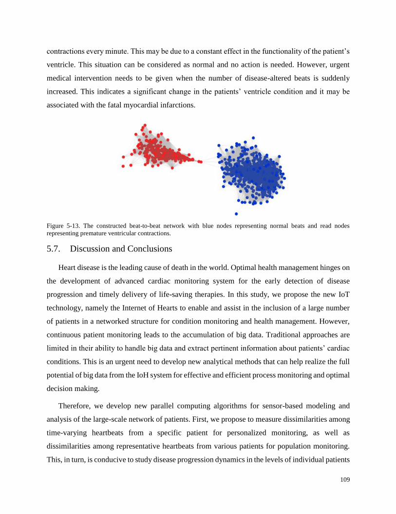
109
contractions every minute. This may be due to a constant effect in the functionality of the patient’s
ventricle. This situation can be considered as normal and no action is needed. However, urgent
medical intervention needs to be given when the number of disease-altered beats is suddenly
increased. This indicates a significant change in the patients’ ventricle condition and it may be
associated with the fatal myocardial infarctions.
Figure 5-13. The constructed beat-to-beat network with blue nodes representing normal beats and read nodes
representing premature ventricular contractions.
5.7. Discussion and Conclusions
Heart disease is the leading cause of death in the world. Optimal health management hinges on
the development of advanced cardiac monitoring system for the early detection of disease
progression and timely delivery of life-saving therapies. In this study, we propose the new IoT
technology, namely the Internet of Hearts to enable and assist in the inclusion of a large number
of patients in a networked structure for condition monitoring and health management. However,
continuous patient monitoring leads to the accumulation of big data. Traditional approaches are
limited in their ability to handle big data and extract pertinent information about patients’ cardiac
conditions. This is an urgent need to develop new analytical methods that can help realize the full
potential of big data from the IoH system for effective and efficient process monitoring and optimal
decision making.
Therefore, we develop new parallel computing algorithms for sensor-based modeling and
analysis of the large-scale network of patients. First, we propose to measure dissimilarities among
time-varying heartbeats from a specific patient for personalized monitoring, as well as
dissimilarities among representative heartbeats from various patients for population monitoring.
This, in turn, is conducive to study disease progression dynamics in the levels of individual patients
110
and the population. It is worth mentioning that there are various ways to measure the pattern
dissimilarity such as correlation, mutual information, and dynamic spatiotemporal warping. These
dissimilarity measures can also be computed in a variety of signal representations such as time
domain, frequency domain, state space domain, or time-frequency domain. Second, we transform
the obtained dissimilarity matrix into the B2B and P2P networks. Indeed, ECG patterns can be
matched between subjects to identify communities, or benchmarked between heartbeats for
personalized health monitoring. For the personalized B2B network, each beat is represented as a
network node and node attributes are ECG patterns within the heartbeat. For the P2P network,
each node represents an individual and node attributes are the salient ECG pattern from this
individual.
However, such network modeling is computationally expensive due to the high volume of data.
Traditional serial computing schemes are limited in their ability for efficient network
representation and real-time analytics in the IoH setting. In this investigation, we developed new
parallel computing algorithms to reduce the computational complexity of network modeling by
distributing the network optimization into multiple processors for fast processing. As such, this is
well suited for modeling and optimization of the large-scale network of patients in the IoH
contexts. Finally, we leverage network features to develop new statistical control charts for real-
time cardiac monitoring.
Notably, multi-level network modeling is a critical component in the IoH that will help
clinicians identify communities that share a similarity in cardiac activity, study disease
mechanisms in each community, and pinpoint a patient in one of the communities. The P2P
network reveals the aggregated information of patients. For example, community detection in the
P2P network will help delineate different types of cardiac conditions. The number of nodes in each
community discloses how many patients are associated with each cardiac condition. The
distribution of nodes in each community shows whether large or small variations exist among
patients in that community. The spatial location of a node (i.e., a patient) helps identify the cardiac
condition. For example, if one node is embedded close to the normal group, it will have a high
probability to be normal. However, if nodes are increasingly embedded close to the diseased group,
a closer attention should be paid to them. Furthermore, the personalized B2B network over time
reveals the progressive variations of cardiac conditions for a specific individual. In this
investigation, multi-level network analytics are shown to have strong potentials for a better

111
understanding of disease mechanisms in various populations and the identification of high-risk
individuals.

112
Chapter 6: Conclusions and Future Research
In recent years, there has been growing interest to investigate increasingly complex systems,
e.g., from conventional machining (~mm) to ultra-precision machining (~nm) and from organs to
cells and genes in the medicine. To address the system complexity, advanced sensing technology
has been used more and more to increase the information visibility and system controllability. In
particular, sensor networks and imaging technology have been more and more used to capture
high-resolution space-time information of the system. Furthermore, the Internet of Things deploys
a multitude of sensors for the continuous monitoring of machine and patient conditions. As a result,
the structure of sensing data has become increasingly complex:
1) Data from individual sensors are with higher dimensionality, e.g., from single-channel to
multi-channel signals and from 1-dimensional profiles to 2- or 3- dimensional imaging
profiles.
2) Data are collected from larger-scale systems, e.g., from a single machine to a large-scale
manufacturing system and from a single patient to the patient population.
In the literature, limited works have been done in industrial engineering to cope with the ever-
increasing complexity of data for system modeling, process monitoring, anomaly detection, and
performance improvement. The methodologies developed in this dissertation are interdisciplinary,
which integrates techniques from engineering domain, statistics, and medicine. Contributions of
this dissertation are summarized as follows:
1) In Chapter 2, a new network approach is developed for the differentiation of disease-altered
patterns in 3-lead VCG signals. i) A new warping algorithm is designed to quantify the
spatiotemporal dissimilarity among VCG recordings. ii) A network embedding approach
is introduced to embed the dissimilarity matrix into a network, which preserves warping
distance among functional recordings. iii) Disease properties are quantitatively associated
with network features that represent disease-altered spatiotemporal patterns underlying 3-
lead VCG signals. The developed approach facilitates the understanding of disease-altered
spatiotemporal patterns in cardiac electrical activity and can be potentially applicable for
the identification of not only myocardial infarctions but also other cardiac disorders.

113
2) In Chapter 3, a new dynamic network scheme is designed and developed to represent,
model, and monitor real-time image data. i) The steam of time-varying images is
represented as a dynamic network. ii) Community structures of the dynamic network are
characterized. iii) A new control chart, namely, the network-generalized likelihood ratio
chart is developed to detect the change point of the underlying dynamics of complex
processes. The developed network scheme has advantageous features to effectively
represent not only 2D images but also higher-dimensional profiles. Thus, the new dynamic
network SPC method is shown to have strong potentials for general applications in diverse
domains with in-situ imaging data.
3) In Chapter 4, a new large-scale network approach is developed for IIoT machine
information processing, condition monitoring, and fault diagnosis. i) We introduce a
stochastic learning approach to significantly improve the computational efficiency of
network embedding and optimize the embedding of each machine in the network. ii) The
stochastic embedding is further parallelized to enable a fast optimization of large-scale
machine networks in the contexts of IIoT. The proposed methodology has a strong potential
to promote existing manufacturing practices towards globalized production optimization
and management. Furthermore, it provides a great opportunity to optimize the energy
consumption and realize green and sustainable manufacturing. In addition, the parallel-
computing approach for network optimization can be potentially applicable to not only
manufacturing but also other research areas such as disease diagnosis and prognosis,
infection prevention and control, supply chain optimization and service networks.
4) In Chapter 5, a new approach of dynamic network modeling is developed for multi-level
cardiac monitoring to realize the Internet of Health Things. i) The IoH, a new IoT-based
cardiac care system is proposed, which integrates IoT sensing, wireless communication,
big data analytics, and medical decision making to realize smart and connected cardiac
health management. ii) A beat-to-beat network is developed to create personalized
baselines and reveal progressive cardiac variations of a specific patient. iii) A patient-to-
patient network is constructed to delineate different types of cardiac conditions among
various patients in the IoH for population-level monitoring. iv) A parallelized stochastic
learning approach is developed to harness the power of multiple processors for fast network
optimization. This enables the inclusion of a large patient population in the IoH for real-

114
time monitoring and disease management. The developed scheme of multi-level network
analytics is shown to have strong potentials for a better understanding of disease
mechanisms in various populations and the identification of high-risk individuals.
Based on the developed methodologies in this dissertation, there are some research topics that
deserve further investigations, including:
Dynamic network monitoring of time-varying image profiles
Network community statistics: In Chapter 3, we extract mean and standard deviation
of pixel intensities, and the number of pixels in each community as features and fed
into the NGLR chart for change point detection. Future studies will be conducted to
extract other types of community statistics. For example, each community is a sub-
network and network topological metrics such as density and clustering coefficient can
be extracted.
Sensitivity analysis and performance comparison: Other methods also have potentials
for online image-based process monitoring, e.g., wavelet analysis. Future studies can
be done to compare the network-based approach and other methods. Also, sensitivity
analysis will be conducted to evaluate the influence of model parameters (e.g., number
of communities and the weight 𝛼) on the performance of change-point detection.
Industrial Internet of Things
Heterogeneous sensor fusion: In Chapter 4, we focus on the analysis of energy profiles
in the IIoT. Instead of one type of sensor, heterogeneous sensors are more and more
used for collaborative monitoring of advanced manufacturing processes. How to
extract useful information from different types of sensors remains a challenge. In the
future, IIoT-based heterogeneous sensor fusion is worth investigating.
Low-volume and high-mix scenario: In Chapter 4, we assume the same type of
products. In other words, we focus on a high-volume and low-mix scenario. Future
works may extend our algorithm to the low-volume and high-mix scenario. That is,
different types of machines are monitored simultaneously in the IIoT. This calls for the
development of new algorithms that incorporate the variations among heterogeneous
machines or products.

115
Internet of Health Things
Beyond morphological features: In Chapter 5, we characterize morphological features
from cardiac signals. Future studies will integrate other types of features (e.g.,
frequency domain features) into the IoH virtual network for disease diagnosis.
Furthermore, the data-rich environment of IoH not only provides cardiac signals but
also other patient data, e.g., blood pressure, respiratory rate, and other vital signs. These
data will also be considered in the IoH in the future.
Advanced parallel computing techniques: In Chapter 4 and 5, the focus is to parallelize
the stochastic network embedding, which is with a sequential nature and difficult to be
directly parallelized. Future studies will continue developing advanced parallel
computing techniques. For example, studies will be done to develop approximate and
probabilistic algorithms to compute sufficiently optimal solutions while using bounded
time, space, communication, and energy; and design new programming logic and
language mechanisms to support existing and new computational models.

116
Appendix
Appendix A – Proof of Proposition 1 in Chapter 3
Proposition 1: If the process is in control, 𝒚(𝑖) is approximately a multivariate normal distribution
as 𝒚(𝑖)~𝑀𝑉𝑁(𝝁0, 𝜮), where 𝝁0 and 𝜮 are in-control mean and covariance matrix of feature vectors.
Proof: Let’s focus on the 𝑘𝑡ℎ community and thus dropping the subscript 𝑘. As the Hamiltonian
approach favors strongly connected nodes into one community, image pixels within each
community are homogeneous. In other words, pixel intensities 𝑥1, 𝑥2, …, 𝑥𝑛 within one community
approximately follow a normal distribution 𝑁(𝜇, 𝜎2) (see Fig. 3-6).
1) By the central limit theorem, 𝑥1, 𝑥2, …, 𝑥𝑛 be random samples from a distribution with finite
mean 𝜇 and variance 𝜎2, the sample mean �̅� follows an approximate normal distribution when
𝑛 is large. That is, the sample mean �̅� of one community from image to image can be
approximated by a normal distribution as �̅�~𝑁(𝜇,𝜎2
𝑛).
2) Notably, ∑ (𝑥𝑖−𝜇
𝜎)2
~𝜒(𝑛)2𝑛
𝑖=1 . If we replace 𝜇 with �̅�, then we have:
∑(𝑥𝑖 − �̅�
𝜎)2
~𝜒(𝑛−1)2
𝑛
𝑖=1
Because 𝑠2 = 1
𝑛−1∑ (𝑥𝑖 − �̅�)2𝑛
𝑖=1 , we have:
∑(𝑥𝑖 − �̅�
𝜎)2𝑛
𝑖=1
=(𝑛 − 1)𝑠2
𝜎2~𝜒(𝑛−1)
2
When 𝑛 is large, the chi-square distribution asymptotically converges to a normal distribution
based on the central limit theorem [106]. In practice, 𝑛 >50 the distribution is sufficiently close
to a normal distribution for the difference to be ignored [107]. In our case, the number of pixels
in each community is much greater than 50.
Further, let 𝑤 =(𝑛−1)𝑠2
𝜎2 and ℎ(𝑤) denotes the probability density function. The expectation of
√(𝑛−1)𝑠
𝜎 is then given as:

117
𝐸 (√(𝑛 − 1)𝑠
𝜎) = ∫ √𝑤ℎ(𝑤)𝑑𝑤
∞
0
= ∫ √𝑤1
2(𝑛−1) 2⁄ 𝛤((𝑛 − 1)/2)𝑤
(𝑛−1)2
−1𝑒−𝑤/2𝑑𝑤∞
0
= √2𝛤(𝑛/2)
𝛤((𝑛 − 1)/2)
Hence,
𝐸(𝑠) = √2
𝑛 − 1
𝛤(𝑛/2)
𝛤((𝑛 − 1)/2)𝜎
In addition,
𝑉𝑎𝑟(𝑠) = 𝐸(𝑠2) − (𝐸(𝑠))2= (1 − (√
2
𝑛 − 1
𝛤(𝑛/2)
𝛤((𝑛 − 1)/2))
2
)𝜎2
Based on the normality assumption, the 𝑠 chart is commonly used to monitor process variance
as follows:
𝑈𝐶𝐿 = 𝑐4𝜎 + 3√(1 − 𝑐42)𝜎
𝐶𝐿 = 𝑐4𝜎
𝐿𝐶𝐿 = 𝑐4𝜎 − 3√(1 − 𝑐42)𝜎
where
𝑐4 = √2
𝑛 − 1
𝛤(𝑛/2)
𝛤((𝑛 − 1)/2)
If the process is in control, the number of pixels 𝑛 within one community randomly fluctuates
around a mean value. Thus, distribution of 𝑛 can be approximated by a normal distribution. The
normal probability plot in Fig. 3-7 shows that the number of pixels of one community from
image to image is approximately normally distributed.∎

118
Appendix B – Proof of Proposition 2 in Chapter 3
Proposition 2: In the eigenspace, multivariate NGLR statistic 𝑅𝑚,𝒚 in Eq. (3-11) is equivalently
computed as:
𝑅𝑚,𝐙 = max𝑚−𝑤≤𝜏<𝑚
𝑚 − 𝜏
2(�̂�𝑚,𝜏,𝐙)
𝑇𝑺𝒛
−1(�̂�𝑚,𝜏,𝐙)
where:
�̂�𝑚,𝜏,𝐙 =1
(𝑚 − 𝜏)∑ 𝐙(𝑖, : )𝑇
𝑚
𝑖=𝜏+1
and 𝐙(𝑖, : )𝑇, 𝑖 = 1,2, … ,𝑚 are principal components obtained by eigen transformation of feature
vector 𝒚(𝑖).
Proof: First, the mean is subtracted from the feature matrix, i.e., 𝐘∗ = [𝒚(1) − �̅�, 𝒚(2) −
�̅�,… , 𝒚(𝑚) − �̅�]𝑇. The 𝑚 × 𝑄 matrix 𝐘∗ is then factorized into three matrices (𝐔, 𝛀 and 𝐕) by
singular value decomposition:
𝐘∗ = 𝐔𝛀𝐕𝑇
where 𝐔 and 𝐕 are 𝑚 × 𝑚 and 𝑄 × 𝑄 orthogonal matrices, 𝛀 is a 𝑚 × 𝑄 diagonal matrix with
diagonal entries 𝜆1 ≥ 𝜆2 ≥ ⋯ ≥ 𝜆𝑄 ≥ 0 (i.e., singular values of 𝐘∗). Each vector in 𝐕 is an
eigenvector that represents a principal component direction of 𝐘∗. Principal components 𝐙 (𝑚 × 𝑄)
are computed by projecting 𝐘∗ onto the eigenvector 𝐕 as:
𝐙 = 𝐘∗𝐕 = 𝐔𝛀𝐕𝑇𝐕 = 𝐔𝛀
Note that the first principal component 𝐙(1, : ) = 𝐘∗𝒗𝟏 has the largest sample variance among all
principal components. The feature covariance matrix 𝑺 becomes:
𝑺 =1
𝑚 − 1∑(𝒚(𝑖) − �̅�)(𝒚(𝑖) − �̅�)
𝑇𝑚
𝑖= 1
=1
𝑚 − 1𝐕𝐙𝑇𝐙𝐕𝑇 = 𝐕𝑺𝒛𝐕
𝑇
where 𝑺𝒛 denotes the covariance matrix of 𝐙. By substituting Eq. (3-7) into (3-11), we have:
(�̂�𝑚,𝜏,𝒚 − �̅�)𝑇𝑺−1(�̂�𝑚,𝜏,𝒚 − �̅�)
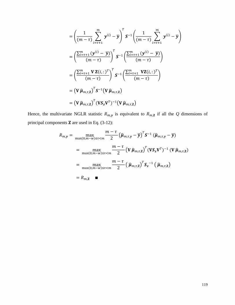
119
= (1
(𝑚 − 𝜏)∑ 𝒚(𝑖)
𝑚
𝑖=𝜏+1
− �̅�)
𝑇
𝑺−1 (1
(𝑚 − 𝜏)∑ 𝒚(𝑖)
𝑚
𝑖=𝜏+1
− �̅�)
= (∑ (𝒚(𝑖)𝑚
𝑖=𝜏+1 − �̅�)
(𝑚 − 𝜏))
𝑇
𝑺−1 (∑ (𝒚(𝑖)𝑚
𝑖=𝜏+1 − �̅�)
(𝑚 − 𝜏))
= (∑ 𝐕 𝐙(𝑖, : )𝑇𝑚
𝑖=𝜏+1
(𝑚 − 𝜏))
𝑇
𝑺−1 (∑ 𝐕𝐙(𝑖, : )𝑇𝑚
𝑖=𝜏+1
(𝑚 − 𝜏))
= (𝐕 �̂�𝑚,𝜏,𝐙)𝑇𝑺−1(𝐕 �̂�𝑚,𝜏,𝐙)
= (𝐕 �̂�𝑚,𝜏,𝐙)𝑇(𝐕𝑺𝒛𝐕
𝑇)−1(𝐕 �̂�𝑚,𝜏,𝐙)
Hence, the multivariate NGLR statistic 𝑅𝑚,𝒚 is equivalent to 𝑅𝑚,𝐙 if all the Q dimensions of
principal components 𝐙 are used in Eq. (3-12):
𝑅𝑚,𝒚 = maxmax(0,𝑚−𝑤)≤𝜏<𝑚
𝑚 − 𝜏
2(�̂�𝑚,𝜏,𝒚 − �̅�)
𝑇𝑺−1 (�̂�𝑚,𝜏,𝒚 − �̅�)
= maxmax(0,𝑚−𝑤)≤𝜏<𝑚
𝑚 − 𝜏
2(𝐕 �̂�𝑚,𝜏,𝐙)
𝑇(𝐕𝑺𝒛𝐕
𝑇)−1 (𝐕 �̂�𝑚,𝜏,𝐙)
= maxmax(0,𝑚−𝑤)≤𝜏<𝑚
𝑚 − 𝜏
2( �̂�𝑚,𝜏,𝐙)
𝑇𝑺𝒛
−1 ( �̂�𝑚,𝜏,𝐙)
= 𝑅𝑚,𝐙 ∎

120
Appendix C – Copyright Permissions
Copyright permission for Chapter 2

121
Copyright permission for Chapter 3

122
123

124

125
126
References
[1] L. Kang and S. L. Albin, "On-line monitoring when the process yields a linear profile," Journal
of Quality Technology, vol. 32, No.4, pp. 418-426, 2000.
[2] K. Kim, M. A. Mahmoud and W. H. Woodall, "On the monitoring of linear profiles," Journal
of Quality Technology, vol. 35, pp. 317-328, 2003.
[3] C. Zou, Y. Zhang and Z. Wang, "A control chart based on a change-point model for monitoring
linear profiles," IIE Transactions, vol. 38, No.12, pp. 1093-1103, 2006.
[4] D. W. Apley, "Discussion of nonparametric profile monitoring by mixed effects modeling,"
Technometrics, vol. 52, No.3, pp. 277-280, 2010.
[5] S. Zhou, Y. Ding, Y. Chen and J. Shi, "Diagnosability study of multistage manufacturing
processes based on linear mixed-effects models," Technometrics, vol. 45, No.4, pp. 312-325,
2003.
[6] K. Paynabar, J. Jin and M. Pacella, "Monitoring and diagnosis of multichannel nonlinear profile
variations using uncorrelated multilinear principal component analysis," IIE Transactions,
vol. 45, No.11, pp. 1235-1247, 2013.
[7] Y. Ding, L. Zeng and S. Zhou, "Phase I analysis for monitoring nonlinear profiles in
manufacturing processes," Journal of Quality Technology, vol. 38, No.3, pp. 199-216, 2006.
[8] H. Yang, "Multiscale Recurrence Quantification Analysis of Spatial Cardiac Vectorcardiogram
Signals," IEEE Transactions on Biomedical Engineering, vol. 58, No.2, pp. 339-347, 2011.
[9] S. Zhou, B. Sun and J. Shi, "An SPC monitoring system for cycle-based waveform signals
using Haar transform," Automation Science and Engineering, IEEE Transactions on, vol. 3,
No.1, pp. 60-72, 2006.
[10] N. Ruschin-Riminia, I. Ben-Gal and O. Maimona, "Fractal geometry statistical process
control for non-linear pattern-based processes," IIE Transactions, vol. 45, No.4, pp. 355-373,
2013.
[11] G. Liu and H. Yang, "Self-organizing network for group variable selection and predictive
modeling," Annals of Operations Research, vol. 33, No.9, pp. 1399-1418, 2017.
127
[12] H. Sun, X. Deng, K. Wang and R. Jin, "Logistic regression for crystal growth process
modeling through hierarchical nonnegative garrote-based variable selection," IIE
Transactions, vol. 48, No.8, pp. 787-796, 2016.
[13] Y. Chen and H. Yang, "Heterogeneous recurrence representation and quantification of
dynamic transitions in continuous nonlinear processes," Eur. Phys. J. B, vol. 89, pp. 155,
2016.
[14] C. Kan, C. Cheng and H. Yang, "Heterogeneous recurrence monitoring of dynamic transients
in ultraprecision machining processes," Journal of Manufacturing Systems, vol. 41, pp. 178-
187, 2016.
[15] R. Jin, C. Chang and J. Shi, "Sequential measurement strategy for wafer geometric profile
estimation," IIE Transactions, vol. 44, No.1, pp. 1-12, 2012.
[16] L. Zhang, K. Wang and N. Chen, "Monitoring wafers' geometric quality using an additive
Gaussian process model," IIE Transactions, vol. 47, No.1, pp. 1-18, 2015.
[17] Z. Du, M. K. Jeong and S. G. Kong, "Band selection of hyperspectral images for automatic
detection of poultry skin tumors," Automation Science and Engineering, IEEE Transactions
on, vol. 4, No.3, pp. 332-339, 2007.
[18] P. Wilcox, T. Horton, E. Youn, et al, "Evolutionary refinement approaches for band selection
of hyperspectral images with applications to automatic monitoring of animal feed quality,"
Intelligent Data Analysis, vol. 18, pp. 25-42, 2014.
[19] H. Yan, K. Paynabar and J. Shi, "Image-based process monitoring using low-rank tensor
decomposition," Automation Science and Engineering, IEEE Transactions on, vol. 12, pp.
216-227, 2015.
[20] F. M. Megahed, L. J. Wells, J. A. Camelio and W. H. Woodall, "A spatiotemporal method for
the monitoring of image data," Quality and Reliability Engineering International, vol. 28,
No.8, pp. 967-980, 2012.
[21] B. Yao, F. Imani, A. Sakpal, E. Reutzel and H. Yang, "Multifractal analysis of image profiles
for the characterization and detection of defects in additive manufacturing," Journal of
Manufacturing Science and Engineering, 2017.

128
[22] F. Tao, Y. Cheng, L. Xu, L. Zhang and B. Li, "CCIoT-CMfg: Cloud computing and Internet
of Things-based cloud manufacturing service system," IEEE Transactions on Industrial
Informatics, vol. 10, No.2, pp. 1435-1442, 2014.
[23] D. Georgakopoulos, P. Jayaraman, M. Fazia, M. Villari and R. Ranjan, "Internet of Things
and edge cloud computing roadmap for manufacturing," IEEE Cloud Computing, vol. 3, No.4,
pp. 66-73, 2016.
[24] F. Tao, Y. Zou, L. Xu and L. Zhang, "IoT-based intelligent perception and access of
manufacturing resource toward cloud manufacturing," IEEE Transactions on Industrial
Informatics, vol. 10, No.2, pp. 1547-1557, 2014.
[25] K. Thramboulidis and F. Christoulakis, "UML4IoT—A UML-based approach to exploit IoT
in cyber-physical manufacturing systems," Computers in Industry, vol. 82, pp. 128-137, 2016.
[26] G. Adamson, L. Wang and P. Moore, "Feature-based control and information framework for
adaptive and distributed manufacturing in cyber physical systems," Journal of Manufacturing
Systems, vol. 43, No.2, pp. 305-315, 2017.
[27] J. Qin, Y. Liu and R. Grosvenor, "A framework of energy consumption modelling for additive
manufacturing using Internet of Things," Procedia CIRP, vol. 63, pp. 307-312, 2017.
[28] Y. Tan, Y. Ng and J. Low, "Internet-of-Things enabled real-time monitoring of energy
efficiency on manufacturing shop floors," Procedia CIRP, vol. 61, pp. 376-381, 2017.
[29] Y. Xu and M. Chen, "Improving Just-in-Time manufacturing operations by using Internet of
Things based solutions," Procedia CIRP, vol. 56, pp. 326-331, 2016.
[30] Y. Ding, P. Kim, D. Ceglarek and J. Jin, "Optimal sensor distribution for variation diagnosis
in multistation assembly processes," IEEE Transactions on Robotics and Automation, vol. 19,
No.4, pp. 543-556, 2003.
[31] C. Pasluosta, H. Gassner, J. Winkler, J. Klucken and B. Eskofier, "An emerging era in the
management of Parkinson’s disease: wearable technologies and the Internet of Things," IEEE
Journal of Biomedical and Health Informatics, vol. 19, No.6, pp. 1873-1881, 2015.

129
[32] M. Al-Taee, W. Al-Nuaimy, Z. Muhsin and A. Al-Ataby, "Robot assistant in management of
diabetes in children based on the Internet of Things," IEEE Internet of Things Journal, vol. 4,
No.2, pp. 437-445, 2017.
[33] S. Islam, D. Kwak, H. Kabir, M. Hossain and K. Kwak, "The internet of things for health
care: a comprehensive survey," IEEE Access, vol. 3, pp. 678-708, 2015.
[34] H. Yang, S. T. S. Bukkapatnam and R. Komanduri, "Spatio-temporal representation of cardiac
vectorcardiogram (VCG) signals," Biomedical Engineering Online, vol. 11, No.16, 2012.
[35] H. Yang, "Multiscale Recurrence Quantification Analysis of Spatial Cardiac
Vectorcardiogram Signals," Biomedical Engineering, IEEE Transactions on, vol. 58, No.2,
pp. 339-347, 2011.
[36] H. Yang, S. T. S. Bukkapatnam, T. Le and R. Komanduri, "Identification of myocardial
infarction (MI) using spatio-temporal heart dynamics," Med. Eng. Phys., vol. 34, No.4, pp.
485-497, 2011.
[37] H. Yang, S. Bukkapatnam and R. Komanduri, "Nonlinear adaptive wavelet analysis of
electrocardiogram signals," Physical Review E, vol. 76, pp. 026214, 2007.
[38] G. E. Dower, A. Yakush, S. B. Nazzal, R. V. Jutzy and C. E. Ruiz, "Deriving the 12-lead
electrocardiogram from four (EASI) electrodes," J. Electrocardiol., vol. 21, No.Supplement
1, pp. S182-S187, 1988.
[39] D. Dawson, H. Yang, M. Malshe, S. T. S. Bukkapatnam, B. Benjamin and R. Komanduri,
"Linear affine transformations between 3-lead (Frank XYZ leads) vectorcardiogram and 12-
lead electrocardiogram signals," J. Electrocardiol., vol. 42, No.6, pp. 622-630, 2009.
[40] Y. Jeong, M. K. Jeong and O. A. Omitaomu, "Weighted dynamic time warping for time series
classification," Pattern Recognit, vol. 44, pp. 2231-2240, 2011.
[41] T. Kohonen, "The self-organizing map," Proceedings of the IEEE, vol. 78, No.9, pp. 1464-
1480, 1990.
[42] M. Hagenbuchner and A. C. Tsoi, "A supervised training algorithm for self-organizing maps
for structures," Pattern Recog. Lett., vol. 26, No.12, pp. 1874-1884, 9, 2005.
130
[43] P. Rao, S. T. S. Bukkapatnam, O. Beyca, Z. Kong and R. Komanduri, "Real-time
identification of incipient surface morphology variations in ultraprecision machining
process," ASME. J. Manuf. Sci. Eng., vol. 136, No.2, pp. 021008-021008-11, 2014.
[44] C. Park, J. Z. Huang, J. X. Ji and Y. Ding, "Segmentation, inference and classification of
partially overlapping nanoparticles," Pattern Analysis and Machine Intelligence, IEEE
Transactions on, vol. 35, No.3, pp. 1-1, 2013.
[45] M. A. Mahmoud and W. H. Woodall, "Phase I analysis of linear profiles with calibration
applications," Technometrics, vol. 46, No.4, pp. 380-391, 2004.
[46] M. A. Mahmoud, P. A. Parker, W. H. Woodall and D. M. Hawkins, "A change point method
for linear profile data," Quality and Reliability Engineering International, vol. 23, No.2, pp.
247-268, 2007.
[47] C. K. H. Koh, J. Shi, W. J. Williams and J. Ni, "Multiple fault detection and isolation using
the Haar transform, Part 2: Application to the stamping process," ASME. J. Manuf. Sci. Eng.,
vol. 121, No.2, pp. 295-299, 1999.
[48] J. Jin and J. Shi, "Feature-preserving data compression of stamping tonnage information using
wavelets," Technometrics, vol. 41, No.4, pp. 327-339, 1999.
[49] S. T. S. Bukkapatnam, A. Lakhtakia and S. R. T. Kumara, "Chaos theory based optimal cutting
tool chatter control," Speculations in Science and Technology, vol. 19, pp. 137-148, 1996.
[50] S. V. Kamarthi, S. R. T. Kumara and P. H. Cohen, "Flank wear estimation in turning through
wavelet representation of acoustic emission signals," ASME. J. Manuf. Sci. Eng., vol. 122,
No.1, pp. 12-19, 2000.
[51] J. Kim, Q. Huang, J. Shi and T. Chang, "Online multichannel forging tonnage monitoring and
fault pattern discrimination using principal curve," ASME. J. Manuf. Sci. Eng., vol. 128, No.4,
pp. 944-950, 2006.
[52] M. K. Jeong and J. Lu, "Wavelet-based SPC procedure for complicated functional data,"
International Journal of Production Research, vol. 44, No.4, pp. 729-744, 2006.
[53] Y. Chen and H. Yang, "Heterogeneous recurrence monitoring and control of nonlinear
stochastic processes," Chaos, vol. 24, No.1, pp. 013138, 2014.
131
[54] M. Newman, "Modularity and community structure in networks," Proc. Natl. Acad. Sci. USA,
vol. 103, No.23, pp. 8577-8582, 2006.
[55] S. Mankad and G. Michailidis, "Structural and functional discovery in dynamic networks with
non-negative matrix factorization," Physical Review E, vol. 88, pp. 042812, 2013.
[56] D. Hu, P. Ronhovde and Z. Nussinov, "Replica inference approach to unsupervised multiscale
image segmentation," Physical Review E, vol. 85, No.1, pp. 016101, 2012.
[57] G. Palla , I. Derényi , I. Farkas and T. Vicsek, "Uncovering the overlapping community
structure of complex networks in nature and society," Nature, vol. 435, pp. 814-818, 2005.
[58] D. Martin, C. Fowlkes, D. Tal and J. Malik, "A database of human segmented natural images
and its application to evaluating segmentation algorithms and measuring ecological statistics,"
in Proceedings of the 8th International Conference on Computer Vision, Vancouver, BC,
July, 2001, pp. 416 - 423.
[59] S. Wang and M. Reynolds, "A GLR control chart for monitoring the mean vector of a
multivariate normal process," Journal of Quality Technology, vol. 45, No.1, pp. 18-33, 2013.
[60] D. Du, H. Yang, S. A. Norring and E. S. Bennett, "Multi-scale modeling of glycosylation
modulation dynamics in cardiac electrical signaling," in Proceedings of 2011 Annual
International Conference of the IEEE Engineering in Medicine and Biology Society (EMBC),
Boston, MA, 2011, pp. 104-107.
[61] D. Du, H. Yang, S. A. Norring and E. S. Bennett, "In-Silico Modeling of Glycosylation
Modulation Dynamics in hERG Ion Channels and Cardiac Electrical Signals," Biomedical
and Health Informatics, IEEE Journal of, vol. 18, No.1, pp. 205-214, 2014.
[62] Z. Wang, S. T. S. Bukkapatnam, S. R. T. Kumara, Z. Kong and Z. Katz, "Change detection
in precision manufacturing processes under transient conditions," CIRP Annals -
Manufacturing Technology, vol. 63, No.1, pp. 449-452, 2014.
[63] C. Cheng, Z. Wang, W. Hung, S. T. S. Bukkapatnam and R. Komanduri, "Ultra-precision
machining process dynamics and surface quality monitoring," Procedia Manufacturing, vol.
1, pp. 607–618, 2015.

132
[64] J. Lee, Y. Shin, M. Kim, et al, "A simplified machine-tool power-consumption measurement
procedure and methodology for estimating total energy consumption," ASME Trans. Journal
of Manufacturing Science and Engineering, vol. 138, No.5, pp. 051004-1-051004-9, 2015.
[65] C. Kan, Y. Chen, F. Leonelli and H. Yang, "Mobile sensing and network analytics for
realizing smart automated systems towards health internet of things," in Automation Science
and Engineering (CASE), 2015 IEEE International Conference on, Gothenburg, Aug. 24-28,
2015, pp. 1072-1077.
[66] J. Jin and J. Shi, "Diagnostic feature extraction from stamping tonnage signals based on design
of experiments," ASME Trans. Journal of Manufacturing Science and Engineering, vol. 122,
No.2, pp. 360-369, 1999.
[67] J. Jin and J. Shi, "Press tonnage signal decomposition and validation analysis for transfer or
progressive die processes," ASME Trans. Journal of Manufacturing Science and Engineering,
vol. 127, No.1, pp. 231-235, 2005.
[68] P. Rao, S. Bukkapatnam, O. Beyca, Z. Kong and R. Komanduri, "Real-time identification of
incipient surface morphology variations in ultraprecision machining process," ASME Trans.
Journal of Manufacturing Science and Engineering, vol. 136, No.2, pp. 021008-1-021008-
11, 2014.
[69] O. Beyca, P. Rao, Z. Kong, S. Bukkapatnam and R. Komanduri, "Heterogeneous sensor data
fusion approach for real-time monitoring in ultraprecision machining (UPM) process using
non-parametric Bayesian clustering and evidence theory," Automation Science and
Engineering, IEEE Transactions on, vol. 13, No.2, pp. 1033-1044, 2016.
[70] P. Rao, J. Liu, D. Roberson, Z. Kong and C. Williams, "Online real-time quality monitoring
in additive manufacturing processes using heterogeneous sensors," ASME Trans. Journal of
Manufacturing Science and Engineering, vol. 137, No.6, pp. 061007-1-061007-12, 2015.
[71] C. Shao, K. Paynabar, T. Kim, et al, "Feature selection for manufacturing process monitoring
using cross-validation," Journal of Manufacturing Systems, vol. 32, pp. 550-555, 2013.
[72] M. Seera, C. Lim, D. Ishak and H. Singh, "Fault detection and diagnosis of induction motors
using motor current signatue analysis and a hybrid FMM-CART model," IEEE Transactions
on Neural Networks and Learning Systems, vol. 23, No.1, pp. 97-108, 2012.
133
[73] S. Emec, J. Kruger and G. Seliger, "Online fault-monitoring in machine tools based on energy
consumption analysis and non-invasive data acquisition for improved resource-efficiency,"
Procedia CIRP, vol. 40, pp. 236-243, 2016.
[74] Y. Liu and X. Xu, "Industry 4.0 and cloud manufacturing: a comparative analysis," ASME
Trans. Journal of Manufacturing Science and Engineering, vol. 139, No.3, pp. 034701-1-
034701-8, 2017.
[75] P. Daugherty, P. Banerjee, W. Negm and A. Alter, "Driving unconventional growth through
the industrial internet of things," New York: Accenture, 2014.
[76] S. Kumara, L. Cui and J. Zhang, "Sensors, networks and internet of things - research
challenges in health care," in IIWeb '11 Proceedings of the 8th International Workshop on
Information Integration on the Web: In Conjunction with WWW 2011, Hyderabad, India,
2011, .
[77] S. Yang, B. Bagheri, H. Kao and J. Lee, "A unified framework and platform for designing of
cloud-based machine health monitoring and manufacturing systems," ASME Trans. Journal
of Manufacturing Science and Engineering, vol. 137, No.4, pp. 040914-1-040914-6, 2015.
[78] N. Raghavan and T. Waghmare, "DPAC: An object-oriented distributed and parallel
computing framework for manufacturing applications," IEEE Transactions on Robotics and
Automation, vol. 18, No.4, pp. 431-443, 2002.
[79] D. Mourtzis, E. Vlachou, N. Milas and N. Xanthopoulos, "A cloud-based approach for
maintenance of machine tools and equipment based on shop-floor monitoring," Procedia
CIRP, vol. 41, pp. 655-660, 2016.
[80] F. Tao, Y. LaiLi, L. Xu and L. Zhang, "FC-PACO-RM: a parallel method for service
composition optimal-selection in cloud manufacturing system," IEEE Transactions on
Industrial Informatics, vol. 9, No.4, pp. 2023-2033, 2012.
[81] H. Yang, C. Kan, G. Liu and Y. Chen, "Spatiotemporal Differentiation of Myocardial
Infarctions," Automation Science and Engineering, IEEE Transactions on, vol. 10, No.4, pp.
938-47, 2013.
[82] H. Yang and G. Liu, "Self-organized topology of recurrence-based complex network," Chaos,
vol. 23, No.4, pp. 043116, 2013.
134
[83] Y. Chen and H. Yang, "Sparse modeling and recursive prediction of space-time dynamics in
stochastic sensor networks," IEEE Transactions on Automation Science and Engineering, vol.
13, No.1, pp. 215-226, 2016.
[84] C. Kan, F. M. Leonelli and H. Yang, "Map reduce for optimizing a large-scale dynamic
network – internet of hearts," in Proceedings of 2016 IEEE Engineering in Medicine and
Biology Society Conference (EMBC), Orlando, FL, 2016, pp. 2962-2965.
[85] P. Demartines and J. Herault, "Curvilinear component analysis: a self-organizing neural
network for nonlinear mapping of data sets," Neural Networks, IEEE Transactions on, vol. 8,
No.1, pp. 148-154, 1997.
[86] M. Li, T. Zhang, Y. Chen and A. Smola, "Efficient mini-batch training for stochastic
optimization," in KDD '14 Proceedings of the 20th ACM SIGKDD International Conference
on Knowledge Discovery and Data Mining, New York, 2014, pp. 661-670.
[87] D. Mozaffarian, E. Benjamin, A. Go, et al, "Heart disease and stroke statistics - 2016 update:
a report from the American Heart Association," Circulation, vol. 136, No.18, 2017.
[88] G. De Luca, H. Suryapranata, J. Ottervanger and E. Antman, "Time delay to treatment and
mortality in primary angioplasty for acute myocardial infarction: every minute of delay
counts," Circulation, vol. 109, No.10, pp. 1223-1225, 2004.
[89] Y. Zhang, Y. Zheng, W. Lin, H. Zhang and X. Zhou, "Challenges and opportunities in
cardiovascular health informatics," IEEE Transactions on Biomedical Engineering, vol. 60,
No.3, pp. 633-642, 2013.
[90] V. Elmberg, J. Almer, O. Pahlm, G. Wagner, H. Engblom and M. Ringborn, "A 12-lead ECG-
method for quantifying ischemia-induced QRS prolongation to estimate the severity of the
acute myocardial event," Journal of Electrocardiology, vol. 49, No.3, pp. 272-277, 2016.
[91] M. Meo, V. Zarzoso, O. Meste, D. Latcu and N. Saoudi, "Spatial variability of the 12-Lead
surface ECG as a tool for noninvasive prediction of catheter ablation outcome in persistent
atrial fibrillation," IEEE Transactions on Biomedical Engineering, vol. 60, No.1, pp. 20-27,
2012.

135
[92] O. Perlman, A. Katz, G. Amit and Y. Zigel, "Supraventricular tachycardia classification in
the 12-Lead ECG using atrial waves detection and a clinically based tree scheme," IEEE
Journal of Biomedical and Health Informatics, vol. 20, No.6, pp. 1513-1520, 2016.
[93] C. Cheng, C. Kan and H. Yang, "Heterogeneous recurrence analysis of heartbeat dynamics
for the identification of sleep apnea events," Computers in Biology and Medicine, vol. 75, pp.
10-18, 2016.
[94] Y. Chen and H. Yang, "Self-organized neural network for the quality control of 12-lead ECG
signals," Physiol. Meas., vol. 33, No.9, pp. 1399, 2012.
[95] H. Yang and F. Leonelli, "Self-organizing visualization and pattern matching of
vectorcardiographic QRS waveforms," Comput. Biol. Med., vol. 79, pp. 1-9, 2016/10, .
[96] S. Man, C. Rahmattulla, A. Maan, et al, "Role of the vectorcardiogram-derived spatial QRS-
T angle in diagnosing left ventricular hypertrophy." Journal of Electrocardiology, vol. 45,
No.2, pp. 154-160, 2012.
[97] M. Yasin, T. Tekeste, H. Saleh, B. Mohammad, O. Sinanoglu and M. Ismail, "Ultra-low
power, secure IoT platform for predicting cardiovascular diseases," IEEE Transactions on
Circuits and Systems-I: Regular Papers, vol. 64, No.9, pp. 2624-2637, 2017.
[98] G. Yang, M. Mantysalo, X. Zhou, et al, "A health-IoT platform based on the integration of
intelligent packaging, unobtrusive bio-sensor, and intelligent medicine box," IEEE
Transactions on Industrial Informatics, vol. 10, No.4, pp. 2180-2191, 2014.
[99] C. Kan and H. Yang, "Internet of hearts - large-scale stochastic network modeling and analysis
of cardiac electrical signals," in Stochastic Modeling and Analytics in Healthcare Systems, J.
Li, N. Kong and X. Xie, Eds. World Scientific, 2017, pp. 211-251.
[100] Z. Eapen, M. Turakhia, M. McConnell, et al, "Defining a mobile health roadmap for
cardiovascular health and disease," Journal of American Heart Association, vol. 5, No.7, pp.
1-6, 2016.
[101] K. Jang, H. Chuang, S. Xu, et al, "Soft network composite materials with deterministic and
bio-inspired designs," Nature Communications, vol. 18, No.6, pp. 1-11, 2015.
136
[102] S. Israel, J. Irvine, A. Cheng, M. Wiederhold and B. Wiederhold, "ECG to identify
individuals," Pattern Recognition, vol. 38, pp. 133-142, 2005.
[103] C. Kan and H. Yang, "Dynamic network monitoring and control of in-situ image profiles
from ultraprecision machining and biomanufacturing processes," Quality and Reliability
Engineering International, 2017.
[104] A. Goldberger, L. Amaral, L. Glass, et al, "PhysioBank, physiotoolkit, and physionet:
Components of a new research resource for complex physiologic signals," Circulation, vol.
23, pp. e215-e220, 2000.
[105] F. Jager, A. Taddei, G. Moody, M. Emdin, G. Antolic and R. Dorn, "Long-term ST database:
a reference for the development and evaluation of automated ischaemia detectors and for the
study of the dynamics of myocardial ischaemia," Medical & Biological Engineering &
Computing, vol. 41, No.2, pp. 172-183, 2003.
[106] D. Horgan and C. Murphy, "On the convergence of the chi square and noncentral chi square
distributions to the normal distribution," IEEE Communication Letters, vol. 17, No. 12, pp.
2233-2236, 2013.
[107] G. Box, J. Hunter and W. Hunter, Statistics for experimenters: design, innovation and
discovery, 2nd ed. New York: Wiley, 2005.
[108] S. de Waele and P. Broersen, "Order selection for vector autoregressive models," IEEE
Transactions on Signal Processing, vol. 51, No. 2, pp. 427-433, 2003.

Vita
Chen Kan
EDUCATION
Ph.D. Industrial and Manufacturing Engineering, Pennsylvania State University, May 2018
MSc. Industrial and Management Systems Engineering, University of South Florida, May 2012
B.Sc. Electrical Engineering, China University of Mining and Technology (Beijing), May 2010
SELECTED PUBLICATIONS
1. C. Kan, Y. Chen, and H. Yang, “Multiscale quality control of telemedicine ECG signal
acquisition,” Telehealthcare Computing and Engineering: Principles and Design, CRC Press, Eds:
Hu Fei, ISBN: 978-1578088027, March 2012.
2. C. Kan and H. Yang, “Internet of Hearts – large-scale stochastic network modeling and analysis
of cardiac electrical signals,” Stochastic Modelling and Analytics in Healthcare Systems, Eds:
Jingshan Li, in press, 2017.
3. C. Kan, C. Cheng and H. Yang, “Heterogeneous recurrence monitoring of dynamic transients in
Ultra-precision machining processes,” Journal of Manufacturing Systems, Vol. 41, pp. 178-187,
2016.
4. C. Cheng, C. Kan and H. Yang, “Heterogeneous recurrence modeling and analysis of heartbeat
dynamics for the identification of sleep apnea events,” Computers in Biology and Medicine, Vol.
75, No. 1, pp. 10-18, 2016.
5. C. Kan, K.P. Yip, and H. Yang, “Two-phase greedy pursuit algorithm for automatic detection and
characterization of transient Calcium signaling,” IEEE Journal of Biomedical and Health
Informatics, Vol. 19, No. 2, pp. 687-697, 2015.
6. H. Yang, C. Kan, G. Liu, and Y. Chen “Spatiotemporal differentiation of myocardial infarctions,”
IEEE Transactions on Automation Science and Engineering, Vol. 10, No. 4, pp. 938-947, 2013.
7. C. Kan S. Kumara and H. Yang, “Fast parallel computing algorithms for large-scale machine
network modeling and condition monitoring,” under 2nd round review, Journal of Manufacturing
Science and Engineering, 2017.
8. C. Kan and H. Yang, “Dynamic network modeling of in-situ image profiles for statistical process
control – applications in ultra-precision machining and bio-manufacturing process,” Quality and
Reliability Engineering International, Vol. 33, No. 8, pp. 2003-2022, 2017.
SELECTED HONORS & AWARDS
2016, Best Paper Finalist, Quality Control and Reliability Engineering Division (QCRE), IIE
Annual Conference, Anaheim, CA.
2015, NSF Travel Grant for presenting at 2015 IIE Annual Conference, Nashville, TN.
2015, Best Paper Finalist, Process Industries Track, 2015 IIE Annual Conference, Nashville, TN.
2015, Featured Article, IEEE Journal of Biomedical and Health Informatics.
2014, The 2nd Place in IIE Mobile App Competition, ISERC 2014, Montreal, Canada.
2014, Entrepreneurial Lead, NSF IIP-1447289, NSF I-Corps Team for the market research and
commercialization of the Mobile E-Network Smart Health (MESH) technology.