dynamic performance of dstatcom used for voltage
TRANSCRIPT
2 0 1 6
Arab Academy for Science, Technology and Maritime
Transport
College of Engineering and Technology
Electrical &Control Engineering
Dynamic Performance of Dstatcom used
for Voltage Regulation in Distribution
System
A thesis submitted to partial fulfilment for the degree of Master
of Science
Presented By:
Mai Sroor Ibrahim Mohamed
Prof. Rania Metwally El-
Sharkawy
Arab Academy for Science and
Technology
Prof. Rizk Mohamed
Hamouda
Faculty of Engineering- Ain Shams
University
.
Arab Academy for Science, Technology and Maritime
Transport
College of Engineering and Technology
Electrical &Control Engineering
Dynamic Performance of Dstatcom used
for Voltage Regulation in Distribution
System
A thesis submitted to partial fulfilment for the degree of Master
of Science
Presented By:
Mai Sroor Ibrahim Mohamed
Prof. Rania Metwally El-Sharkawy Prof. Rizk Mohamed Hamouda
Supervisor Supervisor
Prof.Yasser Galal Prof.Ibrahim Helal
Examiner Examiner

ACKNOWLEDGMENT
First and foremost I am grateful to "Allah the Almighty" for getting me where I am
today and for all the countless blessings he has bestowed on me, indeed he is the one
worthy of all my prayers and eternal gratitude.
I am also grateful to my parents for always being there for me and for being the cause
for everything, I have accomplished until this day. All my success is the answer for your
prayers.
I have been very fortunate to have two remarkable professors as my supervisors namely:
Prof. Rania Metwally El-Sharkawy and Prof.Rizk Mohamed Hamouda
Words always cannot express my gratitude and appreciation for their guidance, patience
and encouragement in every step of this research. I will always be indebted to both of
them for helping me to get this far.
Finally I would like to thank all those who made a valuable support to accomplish this
research one way or the other.

ABSTRACT
The impact of Distributed Static Compensator size and location on the voltage
regulation of a distribution system is investigated in this research work. Possibility of
coordination between Distributed Static Compensator units at different locations in the
system is critical to maximize the benefit from the device and to enhance the system
voltage. Distributed Static Compensator model available in Matlab Simulink is adopted
for the study. This research work focuses on the applications of Distributed Static
Compensator on the distribution facility feeding a combination of dynamic and static
loads.. For the purpose of current analysis, the detailed model of the Distributed Static
Compensator module is utilized with its different control systems tuned to provide the
best dynamic performance of the Distributed Static Compensator, The dynamic
behavior of the Distributed Static Compensator due to switching on a large industrial
load, line outage and voltage sag are presented.
Possible coordination between different compensators for the purpose of achieving the
best system average voltage with minimum reactive compensation is studied. Effect of
Distributed Static Compensator size on the system voltage in case of voltage sag will be
demonstrated. This study is conducted on the IEEE 14 bus system (69 KV/13.8kv)
without any compensation. The results show the effectiveness of using the Distributed
Static Compensator on the system voltage regulation during normal operating
conditions as well as in cases when the system is subjected to abnormal conditions.
System improved performance is depicted.

i
TABLE OF CONTENTS
COLLEGE OF ENGINEERING AND TECHNOLOGY ..................................................................................... 1
LIST OF ACRONYMS/ABBREVIATIONS .................................................................................................. III
LIST OF FIGURES ................................................................................................................................... IV
LIST OF TABLES ..................................................................................................................................... VI
1 INTRODUCTION ............................................................................................................................. 1
1.1 PREFACE .......................................................................................................................................... 1 1.2 UTILIZED POWER SYSTEM TERMINOLGY ......................................................................................... 2
1.2.1 Power System Adequacy ...................................................................................................... 2 1.2.2 Power System Reliability ...................................................................................................... 2 1.2.3 Power System Security.......................................................................................................... 2 1.2.4 Reactive Power Management .............................................................................................. 2 1.2.5 Power System Stability ......................................................................................................... 3
1.3 THESIS MOTIVATION ......................................................................................................................... 3 1.4 THESIS OUTLINE............................................................................................................................... 4
2 LITERATURE SURVEY AND BACKGROUND. ..................................................................................... 6
2.1 AN OVERVIEW OF POWER SYSTEM STABILITY .............................................................................. 6 2.1.1 Voltage Stability ................................................................................................................... 7
2.2 STABILITY STUDY CONDITIONS ............................................................................................................. 8 2.2.1 Steady State Stability ............................................................................................................ 8 2.2.1.1 Steady State Stability Improvement ..................................................................................... 9 2.2.2 Transient Stability ................................................................................................................. 9 2.2.2.1 Transient Stability Improvement ........................................................................................ 11 2.2.3 Dynamic Stability: ............................................................................................................... 12
2.3 COMPARISON BETWEEN THE STABILITY STUDY CONDITIONS...................................................................... 13 2.4 FLEXIBLE A.C TRANSMISSION SYSTEM ........................................................................................ 13 2.5 FACT DEVICES ............................................................................................................................. 14 2.6 TYPES OF FACT DEVICES .................................................................................................................... 15
2.6.1 Series Compensation: ......................................................................................................... 15 2.6.2 Shunt Compensation: ......................................................................................................... 16 2.6.2.1 Static Var Compensator (SVC): ........................................................................................... 17 2.6.2.2 Statcom: ............................................................................................................................. 18
2.7 METHOS OF IDENTIFICATION OF THE WEAKEST BUSBAR ........................................................................... 24 2.7.1 Trial and Error Method: ...................................................................................................... 24 2.7.2 Sensitivity Analysis: ............................................................................................................ 24 2.7.3 Fuzzy Set Theory: ................................................................................................................ 24 2.7.3.1 Fuzzy Set Operations: ......................................................................................................... 27
2.8 IDENTIFICATION OF THE WEAKEST LINE. ................................................................................................ 29
3 SYSTEM MODELING AND IDENTIFICATION OF THE WEAKEST BUSBAR ......................................... 33
3.1 INTRODUCTION ............................................................................................................................... 33 3.1.1 Identification of Weakest Busbar ....................................................................................... 36 3.1.1.1 Trial and Error Method ....................................................................................................... 36 3.1.1.2 Sensitivity Analysis: ............................................................................................................ 39 3.1.1.3 Fuzzy membership : ............................................................................................................ 40
4 SIMULATION OF ADOPTED SYSTEM. ............................................................................................ 48
4.1 CONTROL SYSTEM OF DSTATCOM ....................................................................................................... 48 4.2 SYSTEM VOLTAGE CONTROL USING DSTATCOM UNIT ............................................................................. 51

ii
4.2.1 Compensator located at bus 14 .......................................................................................... 51 4.2.2 Compensator located at bus 12 .......................................................................................... 53 4.2.3 Two Compensators at Bus 12 and Bus 14........................................................................... 54
4.3 RESPONSE OF DSTATCOM ................................................................................................................. 57 4.3.1 Voltage Sag. ....................................................................................................................... 57 4.3.2 Line Outage ........................................................................................................................ 59 4.3.3 Increasing Load................................................................................................................... 62 4.3.3.1 Increasing loads by 20% in addition to start up two large induction motors: .................... 62 4.3.3.2 Increasing and decreasing loads by 20%: ........................................................................... 64 4.3.3.3 Increasing loads by 20% in addition to start up four large induction motors: ................... 66 4.4 Nose Curve .............................................................................................................................. 72
5 RESULTS. ...................................................................................................................................... 79
5.1 SYSTEM VOLTAGE CONTROL USING DSTATCOM UNIT ............................................................................. 79 5.1.1 Compensator located at bus 14: ......................................................................................... 79 5.1.2 Compensator located at bus 12: ......................................................................................... 80 5.1.3 Two Compensators at Bus 12 and Bus 14........................................................................... 80
5.2 RESPONSE OF DSTATCOM .................................................................................................................. 83 5.2.1 Voltage sag ......................................................................................................................... 83 5.2.2 Line outage ......................................................................................................................... 83 5.2.3 Increasing load ................................................................................................................... 85
6 CONCLUSION. ............................................................................................................................... 87
REFERENCES ......................................................................................................................................... 88
APPENDIX A ......................................................................................................................................... 92
APPENDIX B ......................................................................................................................................... 96
APPENDIX C ........................................................................................................................................ 103
APPENDIX D ....................................................................................................................................... 106
iii
LIST OF ACRONYMS/ABBREVIATIONS
FACTS Flexible AC Transmission System
TCSC Thyristor – Controlled Series Capacitor
SSSC Static Synchronous Series Compensator
SVC Static Var Compensator
STATCOM Static Synchronous Compensator
TCR Thyristor Controlled Reactor
TSC Thyristor Switched Capacitor
FIS Fuzzy Inference System
FVSI Fast Voltage Sensitivity Index
TSC
DSTATCOM
Thyristor Switched Capacitor
Distributed Static Synchronous Compensator
iv
LIST OF FIGURES
Figure 1-1:Reactive power management ...................................................................................................... 2 Figure 2-1: Classification of power system stability. ................................................................................... 6 Figure 2-2:TCSC ........................................................................................................................................ 16 Figure 2-3:SSSC......................................................................................................................................... 16 Figure 2-4: Basic structure of SVC and STATCOM. ................................................................................ 17 Figure 2-5:SVC .......................................................................................................................................... 17 Figure 2-6:steady-state V/I and V/Q characteristic of the SVS .................................................................. 18 Figure 2-7:The three-level neutral-point-clamped phase leg...................................................................... 20 Figure 2-8:Three-level flying capacitor phase leg. ..................................................................................... 21 Figure 2-9:Three-level flying capacitor phase leg. ..................................................................................... 21 Figure 2-10: Three-level flying capacitor phase leg. .................................................................................. 23 Figure 2-11:Three-level flying capacitor phase leg. ................................................................................... 23 Figure 2-12:Classical set description ......................................................................................................... 25 Figure 2-13:A possible description of the vague concept "young" by a crisp set. ..................................... 26 Figure 2-15:Four commonly used input fuzzy sets in fuzzy control and modeling. .................................. 26 Figure 2-14:A possible description of the vague concept " young" by a fuzzy set. ................................... 26 Figure 2-16:Union of fuzzy sets A and B. .................................................................................................. 27 Figure 2-17:intersection of fuzzy sets A and B .......................................................................................... 27 Figure 2-18:Complement of fuzzy set A .................................................................................................... 28 Figure 2-19:Bus system model ................................................................................................................... 29 Figure 2-20:FVSI and voltage versus Qload curve to determine voltage collapse ..................................... 32 Figure 3-1:IEEE 14 bus system .................................................................................................................. 34 Figure 3-2:IEEE 14 bus system model ....................................................................................................... 35 Figure 3-3: Voltage membership function ................................................................................................. 41 Figure 4-1:Dstatcom at bus 14 ................................................................................................................... 49 Figure 4-2: Transient current ...................................................................................................................... 49 Figure 4-3: Controller of Dstatcom ............................................................................................................ 50 Figure 4-4: AC voltage regulator ............................................................................................................... 51 Figure 4-5:Voltage at bus 14 when a 20MVAR Dstatcom unit is located at bus no.14 ............................. 52 Figure 4-6:Injected reactive power at bus 14 when a 20MVAR Dstatcom unit is located at bus no.14 .... 52 Figure 4-7:Voltage at bus 14 when a 20MVAR Dstatcom unit is located at bus no.12 ............................. 53 Figure 4-8:Voltage at bus 12 when a 20MVAR Dstatcom unit is located at bus no.12 ............................. 53 Figure 4-9:Injected reactive power at bus 12 when a 20MVAR Dstatcom unit is located at bus no.12 .... 54 Figure 4-10:Voltage at bus 14 when two compensators units are used at bus 12 and bus 14 with 10MVAR
size each ..................................................................................................................................................... 54 Figure 4-11:Voltage at bus 12 when two compensators units are used at bus 12 and bus 14 with 10MVAR
size each ..................................................................................................................................................... 55 Figure 4-12:Injected reactive power at bus 12 and 14 when two compensators units are used at bus 12 and
bus 14 with 10MVAR size each ................................................................................................................. 55 Figure 4-13:Injected reactive power at bus 12 and 14 at different Vref ..................................................... 56 Figure 4-14:Three phase fault on the transmission system level ................................................................ 57 Figure 4-15:Voltage at bus 14 during fault ................................................................................................ 58 Figure 4-16: Consumed reactive power at bus 14 during fault .................................................................. 58 Figure 4-17:System during line outage ...................................................................................................... 59 Figure 4-18: Voltage at bus 14 during line outage ..................................................................................... 61 Figure 4-19: Consumed reactive power at bus 14 during line outage ........................................................ 61 Figure 4-20: System during increasing loads by 20% in addition to two motors ....................................... 62 Figure 4-21:Voltage at bus 14 in case of increasing the load ..................................................................... 63 Figure 4-22:Injected reactive power at bus 14 in case of increasing the load ............................................ 63 Figure 4-23:Simulation block diagram during increasing loads by 20% ................................................... 64 Figure 4-24: Simulation block diagram during decreasing loads by 20% .................................................. 65 Figure 4-25:Voltage at bus 14 in case of increasing and decreasing loads by 20% ................................... 65 Figure 4-26:Reactive power at bus 14 in case of increasing and decreasing loads by 20% ....................... 66 Figure 4-27: IEEE 14 bus system supported by Dstatcom during increasing loads by 20% in addition to
four motors ................................................................................................................................................. 67

v
Figure 4-28:IEEE 14 bus system supported by constant capacitor during increasing loads by 20% in
addition to four motors ............................................................................................................................... 68 Figure 4-29: IEEE 14 bus system supported by capacitive load during increasing loads by 20% in addition
to four motors ............................................................................................................................................. 69 Figure 4-30: Speed of induction motors when system is supported by different types of compensation ... 70 Figure 4-31:Stator current of induction motors when system is supported by different types of
compensation ............................................................................................................................................. 70 Figure 4-32:Torque of induction motors when system is supported by different types of compensation .. 71 Figure 4-33:Voltage at bus 14 when system is supported by different types of compensation .................. 71 Figure 4-34:thevenin circuit ....................................................................................................................... 72 Figure 4-35 : Short circuit current and open circuit voltage at bus 14 ....................................................... 75 Figure 4-36: Short circuit current and open circuit voltage at bus 12 ........................................................ 76 Figure 4-37:Nose cure at bus 14................................................................................................................. 77 Figure 4-38: Nose cure at bus 12................................................................................................................ 78 Figure A-1:Single line diagram for IEEE 14 bus test system ..................................................................... 92

vi
LIST OF TABLES
Table 2-1: Diffrenences between steady state and dynamic stability. ........................................................ 13 Table 3-1:Average voltage and standard deviation at 10 MVAR .............................................................. 37 Table 3-2:Average voltage and standard deviation at 20 MVAR .............................................................. 37 Table 3-3: Average voltage and standard deviation without Compensation .............................................. 38 Table 3-4:Average voltage and standard deviation at 30 MVAR .............................................................. 38 Table 3-5: Average voltage and standard deviation at bus 14 .................................................................... 39 Table 3-6: Sensitivty analysis .................................................................................................................... 40 Table 3-7: Base solution ............................................................................................................................. 43 Table 3-8:Voltage in different cases .......................................................................................................... 44 Table 3-9:Qlosses from load flow in different cases .................................................................................. 45 Table 3-10:Values of A,B and C. ............................................................................................................... 45 Table 3-11:Qlosses at base case and minimum voltage ............................................................................. 46 Table 3-12: Voltage and reactive power losses membership ..................................................................... 47 Table 3-13: Decision S(i) for each bus. ...................................................................................................... 47 Table 4-1:Fast voltage stability index ....................................................................................................... 60 Table 4-2:Average voltage and standard deviation .................................................................................... 74 Table 4-3: Eth, Rth, Xth and Isc calculations at bus 14 ............................................................................. 76 Table 4-4:Eth, Rth, Xth and Isc calculations at bus 12 .............................................................................. 77 Table 5-1:Average voltage and standard deviation when Dstatcom is located at bus 14 ........................... 79 Table 5-2:Injected Qc to approach 1pu at bus 14 ....................................................................................... 80 Table 5-3:Average voltage and standard deviation when Dstatcom is located at bus 12 ........................... 80 Table 5-4:Consumed reactive power when Dstatcom is located at bus 12 and bus 14 .............................. 81 Table 5-5:Total consumed reactive power ................................................................................................. 82 Table 5-6: Total Average voltage and standard deviation .......................................................................... 82 Table 5-7: Consumed reactive power and voltage without compensation at bus 14 during fault .............. 83 Table 5-8:Total consumed reactive power during line outage ................................................................... 84 Table 5-9:Average voltage and standard deviation during line outage ...................................................... 84 Table 5-10:Total consumed reactive power during increasing loads by 20% in addition to two motors ... 85 Table 5-11:Total consumed reactive power during increasing and decreasing loads by 20% .................. 86 Table A-1:Line data-IEEE 14 bus system .................................................................................................. 93 Table A-2:Values of R,L and C in simulation block(PI section line)......................................................... 94 Table A-3: Transformer tap setting data-IEEE14 bus system .................................................................... 94 Table A-4:Shunt capacitor data-IEEE 14 bus system ................................................................................ 95 Table A-5:Bus data-IEEE 14 bus system ................................................................................................... 95 Table B-1:Load flow-14 Bus System ......................................................................................................... 96 Table B-2:Y Bus ...................................................................................................................................... 101 Table C-1: Without compensation-Nose curve for bus 12 ....................................................................... 103 Table C-2:Vref"0.99pu”atbus12-Nose curve for bus 12 ....................................................................... 103 Table C-3:Vref"0.98 pu at bus 14 and 1pu at bus12"- Nose curve for bus 12 ......................................... 104 Table C-4:Without compensation-Nose curve for bus 14 ........................................................................ 104 Table C-5:Vref"0.99pu”atbus12-Nose curve for bus 14 ....................................................................... 105 Table C-6:Vref"0.98 pu at bus 14 and 1pu at bus12"- Nose curve for bus 14 ......................................... 105 Table D-1:20% increasing loads .............................................................................................................. 106 Table D-2:80%decreasing loads ............................................................................................................... 107

vii

1
C h a p t e r O n e
1 INTRODUCTION
1.1 PREFACE
Power systems are often interconnected, forming very large power pools. Operation
of such power systems becomes increasingly complicated due to rapid growth of
loads without a corresponding increase in transmission capability. The active and
reactive power control generally plays a major role in power system.In recent years
power systems, worldwide have grown in size and complexity. The interconnections
between individual utilities have increased, and many power elements have been
required to operate at their maximum limits for long periods of time. Development
in the power industry forced electric utilities to make better use of the available
transmission facilities of their power systems. This resulted increased power
transfer, reduced transmission margins, and diminished voltage stability
margin.Recently power system voltage instability has become one of the power
utility problems gaining a great attention due to its direct or indirect impact on
recent blackout incidents. Power system planning and operation has to deal with a
significant degree of uncertainty about time and location [1]. With the increased
loading of existing power transmission systems, the problem of voltage stability has
become a major concern in power system operation, and also reactive power
optimization has gained more importance. Reactive power compensation in power
systems has to be comprehensive to maintain all voltages within acceptable limits
during both light and heavy load conditions. During light load the system may need
a decrease in the voltage by adding a reactor, on the other hand, during heavy load
conditions, the system might need capacitive reactive power support. The main
objective of an electric power system and its operation is to maintain the system
security while respecting certain constraints imposed on the system [2].
2
1.2 UTILIZED POWER SYSTEM TERMINOLGY
1.2.1 Power System Adequacy
It is theabilityofapowersystemtosupplyconsumers‟electricpowerandenergy
requirements at all times.
1.2.2 Power System Reliability
It is the degree to which the performance of an electrical system results in power
being delivered to consumers within accepted standards and desired amounts.
A reliable supply of power is maintained for vital electrical loads. This is done by
supplying two (or more) sources of power to these loads, providing load shedding of
non-vital loads to avoid overloading the remaining generating capacity, and
supplying redundant equipment from separate power sources and distribution
circuits. The supporting auxiliaries for a piece of equipment shall be supplied from
the same source of power as the main piece of equipment.
1.2.3 Power System Security
It is the ability of a power system to withstand sudden disturbances [3].
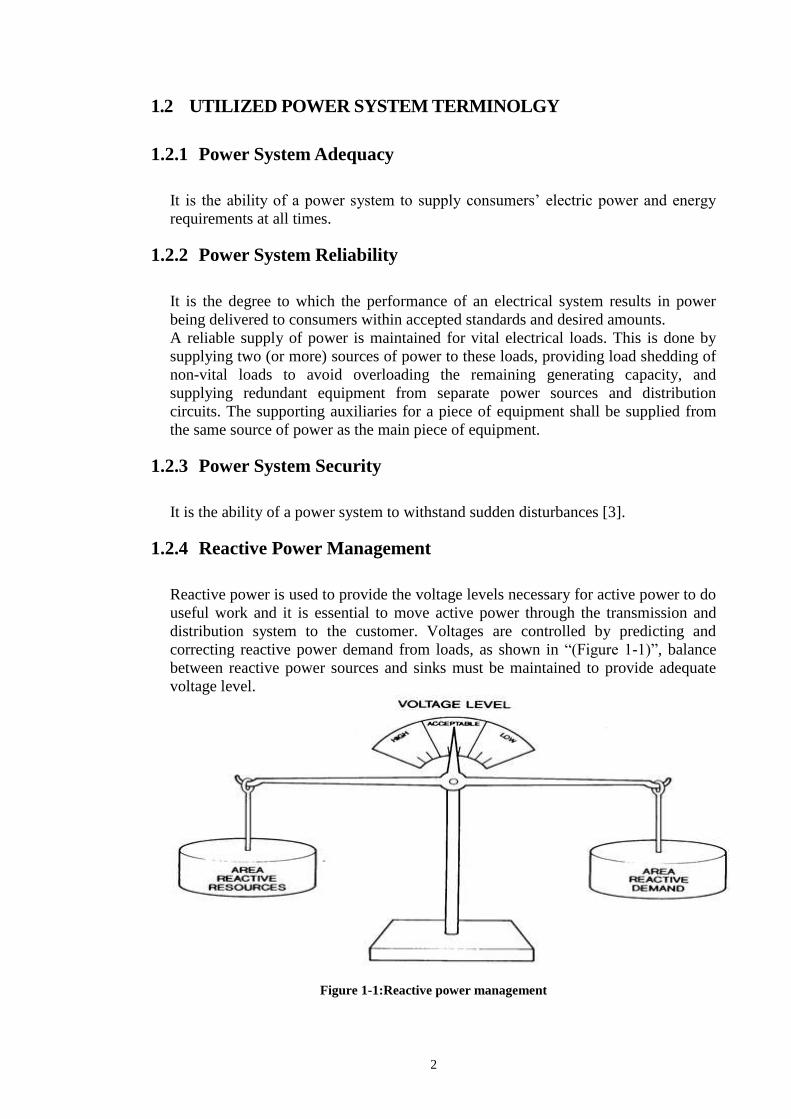
1.2.4 Reactive Power Management
Reactive power is used to provide the voltage levels necessary for active power to do
useful work and it is essential to move active power through the transmission and
distribution system to the customer. Voltages are controlled by predicting and
correcting reactive power demand from loads, as shown in “(Figure1-1)”, balance
between reactive power sources and sinks must be maintained to provide adequate
voltage level.
Figure 1-1:Reactive power management

3
1.2.5 Power System Stability
It is the ability of an electric power system, for a given initial operating condition, to
regain a state of operating equilibrium after being subjected to a physical
disturbance, with system variables bounded so that system integrity is preserved
1.3 THESIS MOTIVATION
Due to the extensive use of highly sensitive electronic equipment, improved power
quality is of great importance for many segments of modern industry. Consumer
expectations regarding environment and the availability of reliable electric power
supply has increased tremendously in the recent years. This has given a thrust to the
development of new equipment that can help in mitigating the power quality
problems. Custom power devices are increasingly being adopted for the purpose of
improving power quality and reliability [4-5]. Thyristor based systems were initially
proposed for reactive power compensation and used for reduction of voltage flicker
due to arc furnace loads [6]. However, due to several disadvantages of passive
devices such as large size, fixed compensation value and possibility of resonance
etc., special attention has been given to the equipment based on the voltage-source
converter (VSC) technology.
The use of compensators with improved qualifications such as distribution static
synchronous compensator, Dstatcom, has garbed researcher's attention for solving
power quality problems. Dstatcom is a compensation device used in a shunt
configuration across the mains of the primary distribution system. Dstatcom makes
use of a voltage source converter and internally generates capacitive (i.e. leading) as
well as inductive (i.e. lagging) reactive power. The use of Dstatcom for solving
problems of voltage sags, flickers and swell…etc have been reported in [7].
Instantaneous reactive power compensator using switching devices have been
reported [8]. References [9-10] listed multifunctional capabilities of Statcom and
presented indirect current control scheme for a Dstatcom [11]. The control system of
the Dstatcom is very fast and has the capability to provide adequate reactive power
compensation to the distribution system [12-13]. Due to this capability, Dstatcom
can be effectively used to regulate voltage drop that occurs during the starting of

4
large loads and/or large induction motors where the required starting current is very
high [14].
None of the previous researches has focused on the possibility of coordination
between compensator devices to achieve the best adjustment of the system voltage.
In the meantime the dynamic behavior of the Dstatcom under different system
disturbances has not been fully explored. This research work focuses on the
applications of Dstatcom on the distribution facility feeding a combination of
dynamic and static loads.. For the purpose of current analysis, the detailed model of
the Dstatcom module is utilized with its different control systems tuned to provide
the best dynamic performance of the Dstatcom.
Determining the location of Dstatcom in the power system is critical to maximize
the benefit from the device. Possible coordination between different compensators
for the purpose of achieving the best system average voltage with minimum reactive
compensation is studied. Effect of Dstatcom size on the system voltage in case of
voltage sag will be demonstrated. Three different techniques are used to determine
the weakest bus and the amount of reactive compensation required to enhance the
system voltage. Moreover, the dynamic performance of the Dstatcom under different
system disturbance is studied and illustrated.
1.4 THESIS OUTLINE
In this research work, the use of Dstatcom in a 14-bus IEEE power system was
modeled, studied and improved performance based on its utilization demonstrated. The
thesis is divided into five chapters:
Chapter one: It starts with a brief introduction, research motivation and thesis
objective.
Chapter two: is an overview of power system stability including the power
stability types and comparing between them, stability study conditions (steady
state, transient and dynamic conditions) and also make comparison between
them. Also this chapter overviews different types of FACTS devices and
explain three methods which are used to identify the best location for any
FACTS device .One of those methods is through trial and error, the second one

5
is by using sensitivity analysis; while the third method is by utilizing fuzzy
rules. This chapter demonstrates that the weakest line in any power system can
be identified by using (Fast Voltage Stability Index).
Chapter three: This chapter shows system modeling and identification of the
weakest bus of IEEE 14 bus system.
Chapter four: This chapter demonstrated simulation results of adopted system
with Dstatcom and the response of this fact device during (fault, line outage and
increasing loads ) .
Chapter five: This chapter demonstrated total consumed reactive power during
normal and abnormal conditions when IEEE 14 bus system supported by
Dstacom and the possible benefits that can be obtained from co-ordination
between more than one compensator in the system also this chapter indicates
that one compensator unit located at the weakest bus has the power to regulate
the system voltage with minimum amount of reactive power comparing to other
buses. More than one unit will not reduce the amount of reactive power required
to enhance the average voltage
Chapter six: Concludes the thesis

6
C h a p t e r T w o
2 LITERATURE SURVEY AND BACKGROUND.
2.1 AN OVERVIEW OF POWER SYSTEM STABILITY
Powersystemstabilitymaybedefinedas“Abilityoftheelectricalpowersystemto
respond to a disturbance frome normal operating condition so as to returning to a
conditionwhere the operation is again normal”[15-16]. Stability is a condition of
equilibrium between opposing forces, therefore the instability may occurs when a
disturbance cause imbalance between the opposing forces. The power system is a
highly nonlinear system that operates in a constantly changing environment; loads,
generator outputs, topology, and key operating parameters change continually.
During the transient disturbance the stability of system depends on the nature of the
disturbance and the initial operating condition. The disturbance may be small or
large. Following a transient disturbance, the power system is stable when it will
reach a new equilibrium state and the system remain intact. The system will keep at
normal state by the actions of automatic controls and possibly human operators. On
the other hand, the system is unstable, when will result in a run-away or run-down
situation for example, a progressive increase in angular separation of generator
rotors, or a progressive decrease in bus voltages. The unstable system condition may
be led to cascading outages and a shut-down of a main portion of the power system.
Instability of the power system can take different forms and is influenced by a wide
range of factors. The power system stability can be classified in to various categories
and subcategories as follow show in“(Figure 2-1)” [17]
Figure 2-1: Classification of power system stability.

7
2.1.1 Voltage Stability
Voltage stability is defined as the "ability of a power system to remain steady
voltages at all buses in the system at normal operating conditions, and after being
subjected to a disturbance". In other word the power system is voltage stable if the
voltages at all buses after disturbance are close to voltages at normal condition
before disturbance. While , it may became unstable if outage of equipments such as
(generator ,line, transformer, bus bar, etc), overload and/or generation decrement
causing weakening of voltage control. Voltage stability is also called load
stability.The main factor causing voltage instability is the inability of the power
system to meet the demands reactive power in the heavily loaded systems to keep
desired voltages [18-19-20]. The voltage stability is classified into two categories:
Small disturbance voltage stability: It is concerned with a system‟s ability to
control voltages after small disturbances such as incremental changes in load. Its
analysis is done in steady state condition.
Large disturbance voltage stability: It is ability of the system to control voltages
following large disturbance such as system faults, loss of generation, or circuit
contingencies [17-19].
.

8
2.2 STABILITY STUDY CONDITIONS
The studies of stability usually classified in to three types depend on the nature and
order of magnitude of the disturbance [15-16]; such as:
2.2.1 Steady State Stability
It is defined as ability of the power system to maintain synchronsim between the
machines of the system and external tie lines following a small slow disturbance
such as (normal load fluctuations , the action of automatic voltage regulators and
turbine governors). Steady state limit is the maximum flow of power through
transmission lines without loss the stability during normal power increasing (
gradually power increasing). Steady state stability and steady state stability limit are
used interchangeably. The power transferred between the alternator and the motor is
expressed as follow, when neglected the losses:
)sin(
X
V mV GPMPG
(2.1)
The maximumpowerwillbetransferredwhenδ=90°.
X
V mV GP
max (2.2)
Where:
VG is the generator voltage terminal.
VM is the motor voltage terminal.
x is the reactance connected between the generator and motor.
δisloadangle.

9
2.2.1.1 Steady State Stability Improvement
From equation (2.2) above the maximum power transfer which flow from generator
to the load (motor) is proportional directly with product of internal voltage of two
machines and proportional inversely to the line reactance (x). Therefore to improve
the stability limit by increasing the maximum power transfer via :
Increasing the excitation of a generator or motor or both to increase the
internal emfs and load angle δ will decrease.
Reducing the transfer reactance by connected more lines in parallel.
2.2.2 Transient Stability
It is defined the ability of the power system to remain stable during the period
following major diturbance such as (transmission system fault, sudden load change ,
loss of generating or line switching). The transient stability studies usually carried
out during short time period may be equal to one swing. Transient stability limit
referred to the ability of the alternator to meet the demand of the loads in power
system. In order to know the system is stable or not, at the power systems have
rotating synchronous machines, usually swing equation is used.
Letangulerdisplacement=ϴradians
Angular velocity (w) = dӨ
dt radians /second.
Angulareacceleration(α)=dw
dt =
d²Ө
dt ² radians⁄second².
Accelerating Power (Pa) = Ta.w watts.
Angular momentum (M) = J w J-s²⁄radian.
Where:
T is Torque in Nm.
J is moment of inertia in kg-m² or J-s²⁄radian².
10
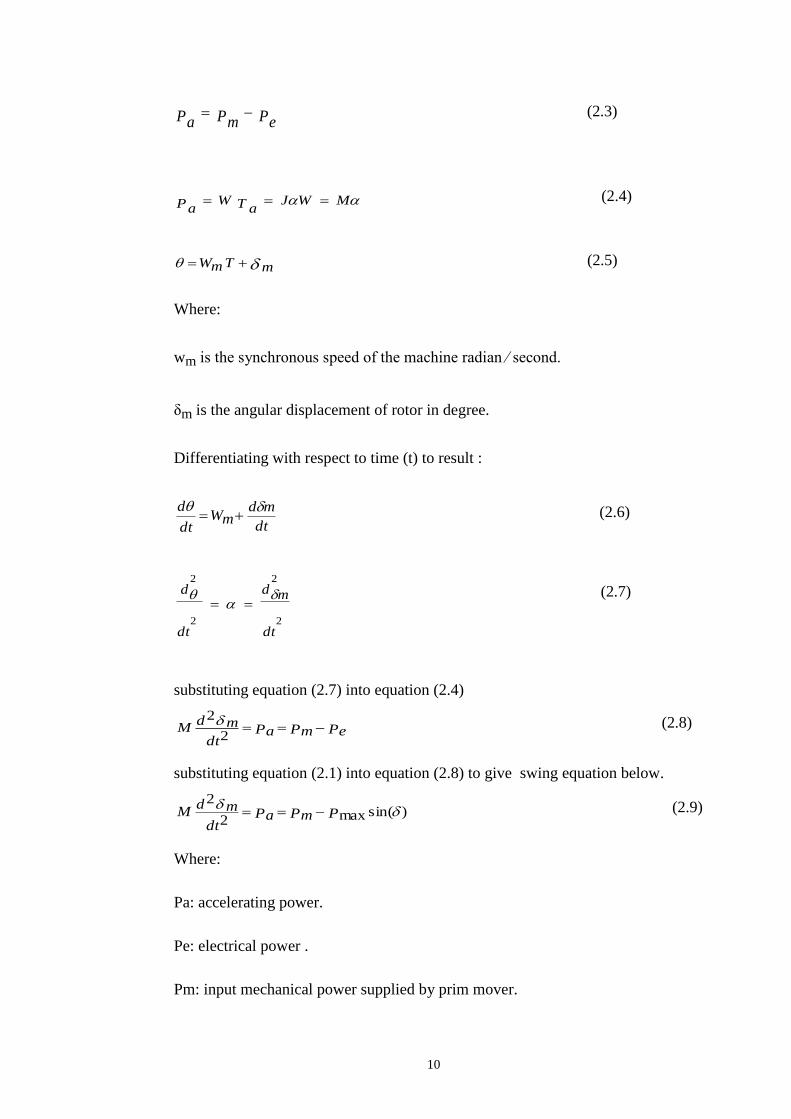
PePmPa (2.3)
MWJT aWPa
(2.4)
mTmW (2.5)
Where:
wm isthesynchronousspeedofthemachineradian⁄second.
δm is the angular displacement of rotor in degree.
Differentiating with respect to time (t) to result :
dt
mdmW
dt
d (2.6)
dt
d m
dt
d
2
2
2
2
(2.7)
substituting equation (2.7) into equation (2.4)
PePmPadt
mdM
2
2 (2.8)
substituting equation (2.1) into equation (2.8) to give swing equation below.
)sin(max2
2
PPmPa
dt
mdM (2.9)
Where:
Pa: accelerating power.
Pe: electrical power .
Pm: input mechanical power supplied by prim mover.

11
MJw (2.10)
From equation (2.10) above M is not constant due to the swing make variation in
(w). In practice assum w = wn where wn is the normal angular velocity of the
machine. Therefore M will consider constant value and call ineritia constant.
2.2.2.1 Transient Stability Improvement
From swing equation there are two factors effected to the transient stability: The
first is the angular swing of the machine during and following the fault conditions.
The second is the critical clearing time.
The methods which utilized to improve the system stability are:
Increasing system voltage: Transient stability is improved by raising the voltage
at generation and load terminals. When the voltage is increased that mean the higher
value of maximum power will transfer through lines of system.
Reduction in transfer reactance: When reducing the transfer reactance will also
increasing the maximum power transfer, therefore the stability also improve. The
line reactance can be reduced via connected more lines in parallel.
High speed circuit breaker and automatic reclosing: To improve the transient
stability and reducing the effect of the fault must be using high speed circuit breaker
to remove the fault at shortest time.
Turbine fast valving.
Application of braking resistors.
Single pole switching.
Quick acting automatic voltage regulators.
12
2.2.3 Dynamic Stability:
It is the ability of the power system to remain in synchronism after the initial swing
(transient stability period) until the system has stable to the new steady state
equilibrium condition. The distinction made between the steady state and dynamic
stability is not clearly because of the stability problems in both the cases are similar,
therefore the two are generally covered under one study. The difference between
them only in the degree of details for modeling of the machines. In dynamic stability
analysis, the excitation systems and the turbine control systems are represented
along with the models of the synchronous machines, but the steady state problems
use very simple generator model which treats the generator as a constant voltage
source. The probability of dynamic instability is much higher than steady state
instability because of the small disturbances are continually occurring on the power
system like small variations, change in turbine speeds ....etc are not big enough to
make the system out of the synchronism [17-21].

13
2.3 COMPARISON BETWEEN THE STABILITY STUDY
CONDITIONS.
“Table2-1” below demonstrate the important differences between the steady state
and dynamic stability and transient stability [21]:
Table 2-1: Diffrenences between steady state and dynamic stability.
Transient stability. Steady state stability and
Dynamic stability.
It is resulting from large sudden
disturbances such as (transmission
system fault, sudden load change , loss
of generation, etc).
It is resulting from small slow
disturbances such as small
changes in load .
Take very short time period that
will be equal to time of one swing (
one second or less).
Lager than period time of
transient stability.
Do not allow the linear analysis to
be used but using nonlinear algebric or
differential equation (such as swing
equation)
Linear mode can be used for
analysis.
Transient stability studies is very
important in power system to ensure
the stability of the system during the
contingency conditions.
Dynamic and steady state
stability studies are less extensive
because of these cases are the
normal conditions of the system .
Improve by several factors such as
increase the system voltage, increas
the maximum power transfer
capability, reduction in transfer
reactance,high speed clearing fault (by
using high speed circuit breaker)
….etc
Improving In steady state by
increasing the excitation of
generator or motor to increase the
maximum power transfer but in
Dynamic stability can be improve
by using proper rating power
system stabilisers.
2.4 FLEXIBLE A.C TRANSMISSION SYSTEM
From ancient time the voltage stability is one of the very important factors in the
power system network. Recently with high development and the significant growth
of the world the study of voltage stability is more and more important. This growth
in the world accompanied by expansion in the electricity networks and increasing

14
demand of electric energy. According to this conditions, the probability of transient,
oscillatory and voltage instability will be increased, which are now brought into
concerns of many utilities especially in planning and operation. Voltage instability is
one of the major reasons which cause voltage collapse in the system. Voltage
collapse may lead to a partial or full power interruption in the system. Power system
network can be modified to alleviate voltage instability or collapse by adding
reactive power sources.
Voltage instability was one of the important reasons for the recent and worst North
American power interruption on August 14th, 2003. The voltage collapse may be
caused by the voltage instability, and voltage collapse may lead to a partial or full
power interruption in the system. The only way to save system from voltage collapse
is to reduce reactive power load or add additional reactive power prior to reach to
collapse point. Therefore reactive power source equipment inserted in the power
system at appropriate location to compensate the reactive power and improve
voltage stability of the system such as (shunt capacitors compensation). Recently
with the evolution in power electronic devices along with developments in control
theory have allowed the design and implementation of structural controllers known
as Flexible a.c transmission system (FACTS). These controller devices used in
power transmission system have led to many applications of them not only to
improve the voltage stability but also to provide operating flexibility to the power
system. Although, (FACTS) devices are quite expensive, they are far better than the
traditional reactive power compensation, as they provide smooth and fast response
to secure power system stability during steady state and transient conditions.
2.5 FACT DEVICES
Flexible AC Transmission Systems, called FACTS, got in the recent years a well-
known term for higher controllability in power systems by means of power
electronic devices. FACTS is defined by the IEEE as" a power electronic based
system and other static equipment that provide control of one or more AC
transmission system parameters to enhance controllability and increase power
transfer capability"[3]. Several FACTS-devices have been introduced for various
applications worldwide. The basic applications of FACTS-devices are:

15
Power flow control.
Increase of transmission capability.
Voltage control.
Reactive power compensation.
Improving voltage stability.
Improving power quality.
Damping of power oscillations.
Improving HVDC link performance.
2.6 TYPES OF FACT DEVICES
2.6.1 Series Compensation:
In series compensation the FACTS are connected in series with the power system. It
works as a controllable voltage source. Therefore the basic principle of all series
FACTS controllers are that they inject voltage in series with the line. In switched
impedance controller, the variable impedance when multiplied with the current flow
through the line represents an injected voltage in the line. It can be used to control
active power flow (P). Series inductance occurs in long transmission lines and when
a large current flow causes a large voltage drop. To compensate, series capacitors
are connected [22-23]. The examples of series compensation are:
Thyristor – Controlled Series Capacitor (TCSC): It is a series capacitor bank is
shunted by a thyristor- controlled reactor shown in “(Figure2-2)”.
Static Synchronous Series Compensator (SSSC): It is a solid-state synchronous
voltage source employing an appropriate dc to ac inverter with Gate Turn-Off
thyristor. It can inject sinusoidal voltage through a transformer connected in series
with the system show in“(Figure2-3)” below.The amplitude and phase angle of this
voltage is variable and controllable [24].

16
Figure 2-2:TCSC
Figure 2-3:SSSC
2.6.2 Shunt Compensation:
In shunt compensation, FACTS is connected in shunt (parallel) with the power
system. It works as a controllable current source. Therefore the basic principle of all
shunt FACTS controllers is injecting current into the system at the point of
connection. It is used to generate or absorb reactive power (reactive power control ).
The most commonly example of shunt compensation are :
Static Var Compensator (SVC).
Static Synchronous Compensator (STATCOM). Shows in“(Figure2-4)” below.

17
Figure 2-4: Basic structure of SVC and STATCOM.
2.6.2.1 Static Var Compensator (SVC):
A static Var compensation scheme with any desired control range can be formed by
using combinations of the elements described above. “(Figure2-5)” shows a typical
SVC scheme consisting of a TCR, a three-unit TSC, and harmonic filters (for
filtering TCR-generated harmonics).At power frequency, the filters are capacitive
and produce reactive power of about 10 to 30% of TCR Mvar rating.
Figure 2-5:SVC
In order to ensure a smooth control characteristic, the TCR current rating should be
slightly larger than that of one TSC unit. “(Figure2-6)” shows The steady-state V/I
characteristic of the SVC and the corresponding V/Q characteristic respectively. The

18
linear control range lies within the limits determined by the maximum susceptance
of the reactor (BLMX), the total capacitive susceptance (BC) as determined by the
capacitor banks in service and the filter capacitance.If the voltage drops below a
certain level (typically 0.3 Pu) for an extended period, control Power and thyristor
gating energy can be lost, requiring a shutdown of the SVC.
The SVC can restart as soon as the voltage recovers. However, the voltage may drop
to low values for short periods, such as during transient faults, without causing the
SVC to trip. The slope reactance XSL has a significant effect on the performance of
the SVC.A large value of XSL makes the SVS less responsive, i.e., changes in
system conditions cause large voltage variations at the SVC high voltage bus. The
value of XSL is determined by the steady-state gain of the controller (Voltage
regulator).
Figure 2-6:steady-state V/I and V/Q characteristic of the SVS
2.6.2.2 Statcom:
The STATCOM is a shunt-connected device with the ability to either generate or
absorb reactive power at a faster rate because no moving parts are involved. It does
not employ capacitor or reactors banks to produce reactive power as the static var
compensator (SVC); the capacitor bank in the STATCOM is used to maintain
constant DC voltage for the voltage-source converter operation .
STATCOM is analogous to an ideal synchronous machine, which generates a
balanced set of three sinusoidal voltages at the fundamental frequency- with
controllable amplitude and phase angle. This ideal machine has no inertia, is

19
practically instantaneous, does not significantly alter the existing system impedance,
and can internally generate reactive (both capacitive and inductive) power.
A STATCOM can improve power-system performance in such areas are the
following:
The dynamic voltage control in transmission & distribution system.
The power oscillation damping in power-transmission system.
The voltage flicker control.
The control of not only reactive power but also ( if needed ) active power in the
connected line; requiring a dc energy source .
Supply reactive power even at low bus voltage
Actually a STATCOM can be classified into two different types voltage source
inverter ( VSI ) and current source inverter ( CSI ). The main different between
the VSI and The CSI, that in VSI the inverter is fed from voltage source and the load
current is forced to fluctuate from positive to negative, and vice versa. To cope with
inductive loads, the power switches with freewheeling diodes are required. Where as
in a CSI, the input behaves as a current source, and the load current is maintained
constant irrespective of load on the inverter and the output voltage is forced to
change There are varieties of STATCOM configureurations, but their composition
are basically the same. Any STATCOM is composed of:
a) inverters with a capacitor or dc source in its dc side: The function of an inverter is to change a dc input voltage to a symmetrical ac
output voltage of desired magnitude and frequency. A variable output voltage can be
obtained by varying the input dc voltage and maintaining the gain of the inverter
constant. On the other hand, if the dc input voltage is fixed and it is not controllable,
a variable output voltage can be obtained by varying the gain of the inverter, which
is normally accomplished by Pulse-Width-Modulation (PWM) control. The output
voltage waveforms of ideal inverters should be sinusoidal, For low and medium-
power applications, square-wave or quasi-square-wave voltage may be acceptable;
and for high-power application, low distorted sinusoidal waveforms are required.
With the availability of high-speed power semiconductor devices, the harmonic

20
contents of output voltage can be minimized or reduced significantly by switching
techniques. The multilevel voltage source inverter is recently applied in many
industrial applications such as ac power supplies, drive systems, etc. One of the
significant advantages of multilevel configureuration is the harmonic reduction in
the output waveform without increasing switching frequency or decreasing the
inverter power output. The output voltage waveform of a multilevel inverter is
composed of the number of levels of voltages, typically obtained from capacitor
voltage sources.
The so-called multilevel starts from three levels. The multilevel inverters can be
classified into three types :
Diode-Clamped Multilevel Inverter (DCMI):The diode-clamped multilevel
inverter uses capacitors in series to divide up the dc bus voltage into a set of voltage
levels. To produce m levels of the phase voltage, an m level diode-clamp inverter
needs m-1 capacitors on the dc bus. The dc bus consists of two capacitors, i.e., C1,
and C2 . For a dc bus voltage Vdc, the voltage across each capacitor is Vdc/2, and
each device voltage stress will be limited to one capacitor voltage level,
Vdc/2,through clamping diodes. DCMI output voltage synthesis is relatively
straightforward. “(Figure 2-7)” explains how the staircase voltage is synthesized,
point O is considered as the output phase voltage reference point. there are three
switch combinations to generate three level voltages across A and O.
Figure 2-7:The three-level neutral-point-clamped phase leg
Output
Switch State
VAO S1 S2 S1\ S2\
V3=Vdc 1 1 0 0
V2=Vdc/2 0 1 1 0
V1=0 0 0 1 1

21
Flying-capacitor Multilevel Inverter (FCMI): “(Figure2-8)” shown below
uses a ladder structure of dc side capacitors where the voltage on each
capacitor differs from that of the next capacitor. To generate m-level
staircase output voltage, m-1 capacitors in the dc bus are needed. Each
phase-leg has an identical structure. The size of the voltage increment
between two capacitors determines the size of the voltage levels in the output
waveform .
Figure 2-8:Three-level flying capacitor phase leg.
Multilevel Inverter Using Cascaded-Inverters with Separated DC
Sources : The general function of this multilevel inverter is the same as that
of the other two previous inverters. The multilevel inverter using cascaded-
inverter with SDCSs synthesizes a desired voltage from several independent
sources of dc voltages as shown in “(Figure2-9)” , which may be obtained
from either batteries, fuel cells, or solar cells. This new inverter can avoid
extra clamping diodes or voltage balancing capacitors.
Figure 2-9:Three-level flying capacitor phase leg.

22
b) Coupling transformers: It is used to couple the inverter to the AC power system. The transformer primary
windings must be isolated from each other, while the secondary windings may be
connected in wye or delta.The transformer secondary is normally connected in wye
toeliminatetriplenharmonics(n=3,6,9,……).
c) DC source: The DC interface provides the interface between the DC side of STATCOM and
other energy sources, Which could be any kind of energy storage device or DC
source, such as wind turbines, DC generator, photovoltaic systems, or other
electronics devices. The traditional STATCOM doesn't have a DC source, it only
has a DC capacitor to maintain its DC side voltage.In theory, the DC capacitor is not
required to be very large. Therefore, the STATCOM is not like a Static Var
Compensator (SVC), whose capacity is mainly determined by the size of capacitor.
The capacitor serves only as a DC source and is necessary for unbalanced system
operation and harmonic absorption. For a STATCOM with energy storage, this DC
capacitor is still required, but its main function is no longer as a DC voltage source,
but as a lower pass filter (harmonic absorption) to reduce the DC current ripple
from/into the DC source.
d) Controller: Mainly the controller of the STATCOM is the controller of a VSI. There are many
topologies to control the VSI voltage. If the switch is capable of operating at higher
frequencies, which is typically the case with fully controlled semiconductors, PWM
concept can be applied.
2.6.2.2.1 Theory Of Operation:
It provides the desired reactive-power generation and absorption entirely by means
of electronic processing of the voltage and current waveforms in a voltage-source
converter (VSC). Where a VSC is connected to a utility bus through magnetic
coupling. A single-line STATCOM power circuit is shown in“(Figure2-10)”.

23
Figure 2-10: Three-level flying capacitor phase leg.
A STATCOM is seen as an adjustable voltage source behind a reactance, this
meaning that capacitor banks and shunt reactors are not needed for reactive-power
generation and absorption, thereby giving the STATCOM a compact design, or
small footprint, as well as low noise and low magnetic impact. The exchange of
reactive power between the converter and the ac system can be controlled by
varying the amplitude of the 3-phase output voltage, Es of the converter, if the
fundamental of the inverter output voltage (Es) is in phase with the utility bus
voltage (Et ). When the amplitude of the output voltage is increased above that of
the utility bus voltage, Et, then current flows through the reactance from the
converter to the ac system and the converter generates capacitive-reactive power for
the ac system.If the amplitude of the output voltage is decreased below the utility
bus voltage, then the current flows from the ac system to the converter and the
converter absorbs inductive-reactive power from the ac system.If the output voltage
equals the ac system voltage, the reactive-power exchange becomes zero, in which
case the STATCOM is said to be in a floating state as shown in“(Figure2-11)”.
Figure 2-11:Three-level flying capacitor phase leg.

24
2.7 METHOS OF IDENTIFICATION OF THE WEAKEST
BUSBAR
2.7.1 Trial and Error Method:
In this method, several trials with different size of fixed reactive compensator at
different location have been considered. In every trial, the average value of the
system voltage and the voltage standard deviation are calculated.The best location
(weakest busbar) is identified as that at which the average voltage is the best with
minimum standard deviation.
2.7.2 Sensitivity Analysis:
The basic equation(2.11) used in Newton-Raphson method is
43
21
VA
Aa
JJ
JJ
Q
P
(2.11)
Where J is the Jacobian Matrix. The reactive power is less sensitive to changes in
phase angles and is mainly dependent on changes in voltage magnitudes [25].
Similarly, real power change is less sensitive to the change in the voltage magnitude
and is most sensitive to the change in phase angle. So, it is quite accurate to set J2
and J3 of the Jacobian matrix to zero. The diagonal elements of J4 indicate the
reactive power sensitivity of i-th bus. ∂Qi/∂|Vi| also indicates the degree of
weakness for the ith bus.
2.7.3 Fuzzy Set Theory:
The traditional set theory (classical set) deal with only one value membership 0 or 1.
The object wholly includes or wholly excludes without partial membership. Crisp
sets handle black-and-white concepts, for example, the classical set of days of the
week unquestionably includes Monday, Thursday, and Saturday. It just as
unquestionably excludes butter, liberty, and dorsal fins, and so on show
“(Figure2-12)” below.

25
Figure 2-12:Classical set description
During the development of the world all the systems which surroud us are complex.
This complexity arises from uncertainty in the form of ambiguity. Therefore the
classical set theory are not sufficient to realistically describe vague concepts[25,26] .
In 1965 Fuzzy set theory was proposed by Professor L. A. Zadeh which deal with
uncertainty problems [27]. A classical set is defined by crisp boundaries, i.e., there is
no uncertainty in the prescription or location of the boundaries of the set. But fuzzy
set defined as a fuzzy set consists of a universe of discourse and a membership
function that maps every element in the universe of discourse to a membership value
between 0 and 1. Where the input space somtimes is referred to as the universe of
discourse. A fuzzy set is in contrast with classical, or crisp sets because members of
a crisp set would not be members unless their membership was full, or complete, in
that set (i.e., their membership is assigned a value of 1). In other hand, the
membership elements in a fuzzy set not necessary to be complet. Elements of a
fuzzy set are mapped to a universe of membership values on the interval 0 to 1. If an
element of universe, say x, is a member of fuzzy set A, then the membership is
given by µA(x) ∈ [0, 1] . One of the most commonly used examples for explain the
crisp set and fuzzy set memberships is the concept of the "young". The age of any
specific person is accurate. However, classifying the age is "young" or not is
involves fuzziness and is sometimes confusing and difficult. Therefore crisp set with
sudden change membership value from 1 to 0 at age 35 is unreasonable, Show
“(Figure2-13)”. In Fuzzy set, an age to "young" relates with a membership value
ranging from 0 to 1. For instance, one might think that age 10 is "young" with
membership value 1, age 30 with membership value 0.75, age 50 with membership
value 0.1, and so on. Show “(Figure2-14)” below .

26
Figure 2-13:A possible description of the vague concept "young" by a crisp set.
There are several types of fuzzy membership function, the most famous types of
membership functions which are needed in most circumstances: trapezoidal,
triangular (a special case of trapezoidal),Gaussian, and bell-shaped. All these fuzzy
sets are continuous, normal, and convex show “(Figure2-15)” below. Among the
four, the first two are more widely used. In this thesis trapezoidal memberships are
used.
Figure 2-15:Four commonly used input fuzzy sets in fuzzy control and modeling.
Figure 2-14:A possible description of the
vague concept " young" by a fuzzy set.
27
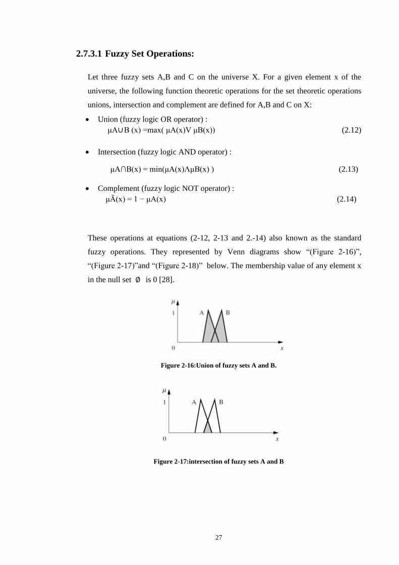
2.7.3.1 Fuzzy Set Operations:
Let three fuzzy sets A,B and C on the universe X. For a given element x of the
universe, the following function theoretic operations for the set theoretic operations
unions, intersection and complement are defined for A,B and C on X:
Union (fuzzy logic OR operator) :
μA∪B(x)=max(μA(x)VμB(x)) (2.12)
Intersection (fuzzy logic AND operator) :
μA∩B(x)=min(μA(x)ΛμB(x)) (2.13)
Complement (fuzzy logic NOT operator) :
μᾹ(x)=1− μA(x) (2.14)
These operations at equations (2-12, 2-13 and 2.-14) also known as the standard
fuzzy operations. They represented by Venn diagrams show “(Figure 2-16)”,
“(Figure2-17)”and “(Figure2-18)” below. The membership value of any element x
in the null set ∅ is 0 [28].
Figure 2-16:Union of fuzzy sets A and B.
Figure 2-17:intersection of fuzzy sets A and B

28
Figure 2-18:Complement of fuzzy set A
Fuzzy Cartesian Product
Let A be a fuzzy set on universe X and B be a fuzzy set on universe Y , then the
Cartesian product between fuzzy sets A and B will result in a fuzzy relation R which
is contained with the full Cartesian product space
A x B=R ⊂ X x Y
where the fuzzy relation Rhas membership function.
μR(x,y)) = μAxB(X,Y)=min(μA (X), μB (Y))
Each fuzzy set could be thought of as a vector of membership values; each value is
associated with a particular element in each set. For example, for fuzzy set A that
has four elements, hence column vector size 4 × 1 and for fuzzy set (vector) B that
has five elements, hence a row vector of 1 × 5. The resulting fuzzy relation R will be
represented by a matrix of size 4 × 5 (i.e.,) R will have four rows and five columns.
Fuzzy Cartesian Composition
Let R be a fuzzy relation on the Cartesian space X ×Y , S be a fuzzy relation
on Y × Z, and T be a fuzzy relation on X × Z, then the fuzzy set max–min
composition is defined as: T= RoS
={ (x, z) , max y{ min _(μR (x, y) , μS (y, z)} /x ∈ X, y ∈ Y z ∈ Z}

29
2.8 IDENTIFICATION OF THE WEAKEST LINE.
Voltage stability index proposed by I.Musirin et al. [29] can be conducted on a
system by evaluating the voltage stability referred to a line. The voltage stability
index referred to a line is formulated from the 2-bus representation of a system. The
voltage stability index developed is derived by first obtaining the current equation
through a line in a 2-bus system. Representation of the system illustrated in “(Figure
2-19)”
Figure 2-19:Bus system model
V1, V2 = voltage at the sending and receiving buses.
P1, Q1 = active and reactive powers at the sending bus.
P2, Q2 = active and reactive powers at the receiving bus.
S1, S2 = apparent powers on the sending and receiving buses.
δ=angledifferencebetweenthesendingandreceivingbuses(δ1– δ2).
Bytakingthesendingendbus,bus1,asthereference(i.e.δ1=0andδ2=δ),then
the general current relationship can be written as;
JXR
VV
I
2
01
(2.15)
Where R is the line resistance and X is the line reactance.The apparent power at bus2
( the receiving end power) can be written as:

30
IVS 22
(2.16)
2
22
2
2
V
QjP
V
SI
(2.17)
Equating (2.15) and (2.17) we obtained,
2
2221 0
V
QjP
JXR
VV
(2.18)
)( )(22
2
221 jXRQjPVVV
(2.19)
Separating the real part and imaginary parts yields
)22
2
221 ( QXRPVCosVV
(2.20)
And
)22
2
221 ( QRPXVSinVV
(2.21)
Rearrange equation(2.21) and substitute at (2.20) yields ), the voltage quadratic
equation at the receiving end bus is written as;
02
)
2
(21
)cossin(2
2 Q
X
RXVV
X
RV (2.22)
2
2)2
(42]1)cossin
[(1)cossin
(
2
QX
RXV
X
RV
X
R
V
(2.23)
ToobtainrealrootsforV2,thediscriminatorissetgreaterthanorequalto„0‟;i.e.:
12
)cossin).(2
1(
.2
.2
.4
XRV
XQZ
(2.24)

31
The angle differenceδisnormallyverysmallthen,
δ≈0,Rsinδ≈0,Xcosδ≈X
Taking the symbols “i” as the sending bus and”j” at the receiving bus ,the fast
voltage stability index,FVSI can be identify
XV
QZFVSI
.2
.2.4
1
212
(2.25)
Where:
Z=line impudence
X=line reactance
Q2=reactive power at the receiving end
V1=Sending end voltage
The line that exhibits FVSI closed to 1.0 implies that it is approaching its instability
point. If FVSI goes beyond 1.0, one of the buses connected to the line will
experience a sudden voltage drop leading to system collapse.Critical line is defined
as that line which when removed from the system might lead to a voltage collapse.
The scenario of system blackout due to voltage collapse can be illustrated as shown
in “(Figure2-20)”. The occurrence of voltage collapse is initiated by voltage drop at
certain bus due to load increase not supported by local power reactive or other
elements support to improve the voltage performance.

32
Figure 2-20:FVSI and voltage versus Qload curve to determine voltage collapse
From the graph, it is shown that as the reactive power loading at a particular load
bus is increased; the FVSI value of the highest sensitive corresponding connecting
line was also increased accordingly. The increase of reactive power loading will also
cause to the voltage profile to decrease until reaching the collapse point. At this
point, the reactive power increase is called as the maximum allowable load or also
termed as maximum loadability. Any attention to continue increasing the reactive
power loading after maximum loadability, voltage will drop accordingly which
would lead to the whole system.

33
C h a p t e r T h r e e
3 SYSTEM MODELING AND IDENTIFICATION OF
THE WEAKEST BUSBAR
3.1 INTRODUCTION
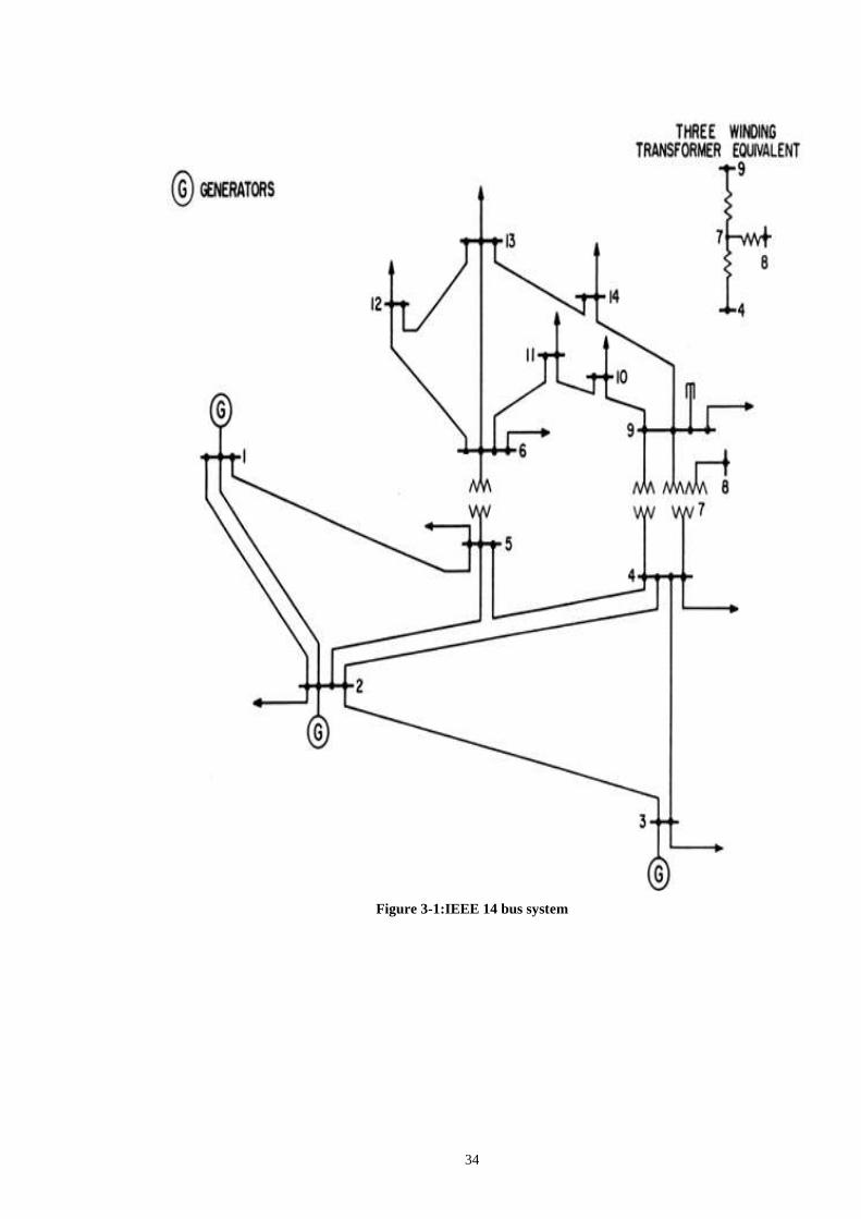
MATLAB simulink program is used for IEEE 14 Bus system (69 kv /13.8kv)
without any compensation. The test system shown in “(Figure3-1)” has 14 buses.
These buses are inter connected via transmission lines, each represented in the form
of a (pi) model. Bus1 is a slack bus, bus 2& bus 3 are a PV bus and other buses are
load buses. The detailed system data is shown in Appendix (A). By logic generators
not allowed to connect directly to any bus bar so the three generators are far a way
from the system by 100km which represented by (Pi section) asshownin“(Figure
3-2)” that grantees that the system will be supported by generators if there is any
problem in one of these lines. The value of R,Land C of others pi sections that
connected between buses is calculated as shown in Appendix (A). There are two
main steps to model this system ;the first one is tuning three generators to give the
required voltage, reactive power and active power in bus 1, 2 and 3 as shown in the
load flow ,see Appendix (B);the other step is tuning transformers that represented by
(Star Grounded –Delta) to give 13.8kv.
34
Figure 3-1:IEEE 14 bus system

35
Figure 3-2:IEEE 14 bus system model

36
3.1.1 Identification of Weakest Busbar
The increase in power demand and limited sources for electric power has resulted in
an increasingly complex interconnected system, forced to operate closer to the limits
of stability. Voltage instability is mainly associated with reactive power imbalance.
the weakest bus in the system and the critical line referred to a bus where the
weakest bus is the best location for Fact devices where they are used to enhance the
power system stability and support the voltage by compensation of reactive power.
This thesis investigates the voltage system stability enhancement by using FACT
device such as DSTATCOM. Practically the location of any FACT device in the
power system is very important factor to give the best results so we use three
methods to know the best location for Dstatcom such as trial and error, Sensitivity
analysis and fuzzy logic control. the weakest bus is the best location for Dstatcom.
3.1.1.1 Trial and Error Method
In this method, several trials with different size of fixed reactive compensator at
different location have been considered. In every trial, the average value of the
system voltage and the voltage standard deviation are calculated. The best location
(weakest busbar) is identified as that at which the average voltage is the best with
minimum standard deviation. Using trial and error method, bus 14 has been found to
have the best average voltage and the minimum standard deviation. This means it is
the weakest bus and the best location for any FACT device.
“Table 3-1”, “Table 3-2”, “Table 3-3”and “Table 3-4” show the system average
voltage and the corresponding standard deviation when load buses are injected by
different values of reactive power (10 MVAR-20MVAR-30MVAR). It is observed
that 20MVAR reactive compensator unit has been chosen for the rest of the analysis
unless otherwise stated.

37
Table 3-1:Average voltage and standard deviation at 10 MVAR
10 MVA at bus Bus
voltage
p.u
System average voltage
System standard
deviation
4 0.980 0.9797857143 0.02935783802
5 0.986 0.9797857143 0.02948408426
6 1.004 0.9876428571 0.02625590313
7 0.987 0.9860714286 0.02639389617
8 1.004 0.987 0.02695763873
9 0.975 0.9876428571 0.02509868279
10 0.976 0.9882571429 0.02482972626
11 0.991 0.9887142857 0.02533046887
12 1 0.9890714286 0.02600676913
13 0.988 0.989 0.02549229575
14 0.971 0.9835714 0.02385553887
Table 3-2:Average voltage and standard deviation at 20 MVAR
20 MVA at bus Bus
voltage
p.u
System average voltage
System standard
deviation
4 1.022 0.9927857143 0.02578531856
5 1.024 0.9928571429 0.02592807949
6 1.036 1.007857143 0.02162953385
7 1.015 1.004571429 0.02101942736
8 1.048 1.006357143 0.02399883075
9 1.016 1.007785714 0.01852865954
10 1.018 1.009285714 0.01837866998
11 1.029 1.009785714 0.0201961049
12 1.044 1.010285714 0.02305716056
13 1.026 1.010285714 0.02117757767
14 1.014 1.011 0.01744788157

38
Table 3-3: Average voltage and standard deviation without Compensation
30 MVA at bus Bus
voltage
pu
System average voltage
System standard
deviation
4 0.974
5 0.980
6 0.980
7 0.966
8 0.966 0.9754285714 0.0313271089
9 0.952
10 0.95
11 0.960
12 0.963
13 0.957
14 0.934
Table 3-4:Average voltage and standard deviation at 30 MVAR
30 MVA at bus Bus
voltage
pu
System average voltage
System standard
deviation
4 1.052 1.000071429 0.0231469352
5 1.055 0.9968571429 0.0242423983
6 1.061 1.021642857 0.0208724591
7 1.057 1.017214286 0.0180877960
8 1.083 1.019571429 0.0248156468
9 1.053 1.021857143 0.0148172541
10 1.057 1.024 0.0156889406
11 1.059 1.0245 0.0190815917
12 1.079 1.025071429 0.0247370869
13 1.056 1.025214286 0.0212339975
14 1.049 1.026 0.01744788157

39
Table 3-5: Average voltage and standard deviation at bus 14
MVAR at bus 14 System average voltage
System standard
deviation
Without compensation 0.9754 0.03132
10 MVAR 0.98357 0.02385
20 MVAR 1.011 0.01744
30 MVAR 1.026 0.01600
It is observed from and “Table3-5” that 20MVAR reactive compensator unit has
been chosen for the rest of the analysis unless otherwise stated.
3.1.1.2 Sensitivity Analysis:
The diagonal elements of J4 in equation indicate the reactive power sensitivity of i-
th bus. ∂Qi/∂|Vi| also indicates the degree of weakness for the ith bus [30],as
∂Qi/∂|Vi| is high and ∂|Vi| /∂Qi becomes low, indicating a minimum change in
voltage for variation Q (reactive power) of the bus ;thus The bus corresponding to
the maximum valueof∂Qi/∂|Vi| is thestrongestbusand thebuscorresponding to
theminimumvalueof∂Qi/∂|Vi|istheweakestbus.Inthismethod weakest load bus
of any multi bus system can be defined [31]. The ith diagonal element of the matrix
[J]-1 also indicates the Q-V sensitivity of load bus i.
According to Appendix (A) and Appendix(B) equation (3.1) is calculated and The
results of the sensitivity analysis on the system under study without any
compensation are shown in “Table3-6”.
ij jiijSin
ijY
jV
iiY
iV
iV
ii
Sin 2- =i
Q
(3.1)

40
Table 3-6: Sensitivty analysis
Bus ∂Qi/∂|Vi|
1 20.95823
2 31.224425
3 9.91839
4 37.1510577
5 33.9268
6 17.1937344
7 18.9865
8 5.483982
9 23.0004856
10 13.959
11 8.13439585
12 5.210665963
13 10.15545
14 4.936575
From the obtained results, it is obvious that ∂Qi/∂|Vi|at bus no.14 is very small and
∂|Vi|/∂Qi becomes high, indicating a maximum change in voltage for variation Q
(reactive power) at this bus ;so bus no.14 is the most sensitive bus in the system and
bus no.12 is the second one ;so bus no.14 is the weakest bus and followed by bus
no.12.
3.1.1.3 Fuzzy membership :
An approach based on fuzzy set theory and heuristic rules to determine the weak
buses in a system is the following: Two membership functions are chosen, the first
one is for reactive power loss, while the second one is for voltage sensitivity. The
voltage membership function is assumed to be in the form of “(Figure3-3)”, which
is described by:

41
max;0
maxmin;1
min0;
min
)(
VV
VVV
VV
V
V
Vi
u (3.2)
Figure 3-3: Voltage membership function
where Vmin and Vmax is the minimum and maximum voltage assigned for each bus
respectively; V is the bus voltage,while the membership function for the reactive
power losses has the same form of “(Figure3-3)”, and is described by the following
equations:
;0
min;
min
min;1
;0
)(
aQ
aQlossQV
QVa
Qa
QVloss
Qbase
Q
baseQ
lossQ
lossQ
iu
(3.3)
Qbase is the total bus reactive power losses at the base load, the nominal operating
load. QVmin is the reactive power loss corresponding to the minimum bus voltage,
and is calculated using the relation between Q and V given by Equation (3.5), and a
is the reactive power losses at V = 0.

42
A fuzzy decision S is chosen for each bus i given by the fuzzy multiplication of
Equations (3.2) and Equations (3.3) as:
(3.4)
Buses having the lowest values of S are specified as weak buses. In the following
section, the steps of identification of weak buses are explained.
Here we will discuss the algorithm solution. Assume that data necessary for system
steady state load flow are available in Appendix (B)., in this case. The following
steps are used for identifying the weak buses.
Step 1. Calculate the load flow for the system base case, that is, the load flow at
normal loading condition. Determine the system active and reactive losses from the
solution of load flow, by using the voltage and angle at eachbusasshownin“Table
3-7”.
))(),(min()()()( iq
uiv
uiq
uiv
uiS

43
Table 3-7: Base solution
Bus Voltage Load Genera tion
Bus(i) Magnitude
(p.u)
Angle
Degree
MW Mvar MW Mvar
1 1.060 0.00 0.00 0.00 233.913 36.693
2 1.025 -4.795 21.700 12.70 40.000 33.038
3 0.990 -13.026 94.200 19.100 0.00 38.860
4 0.974 -10.060 47.800 -3.900 0.00 0.00
5 0.980 -8.494 7.600 1.600 0.00 0.00
6 0.980 -14.808 11.200 7.500 0.00 0.00
7 0.966 -13.511 0.00 0.00 0.00 0.00
8 0.966 -13.511 0.00 0.00 0.00 0.00
9 0.952 -15.410 29.500 16.600 0.00 0.00
10 0.95 -15.645 9.000 5.800 0.00 0.00
11 0.960 -15.374 3.500 1.800 0.00 0.00
12 0.963 -15.833 6.100 1.600 0.00 0.00
13 0.957 -15.907 13.800 5.800 0.00 0.00
14 0.934 -16.849 14.900 5.000 0.00 0.00
Total 259.300 73.600 273.91 108.590
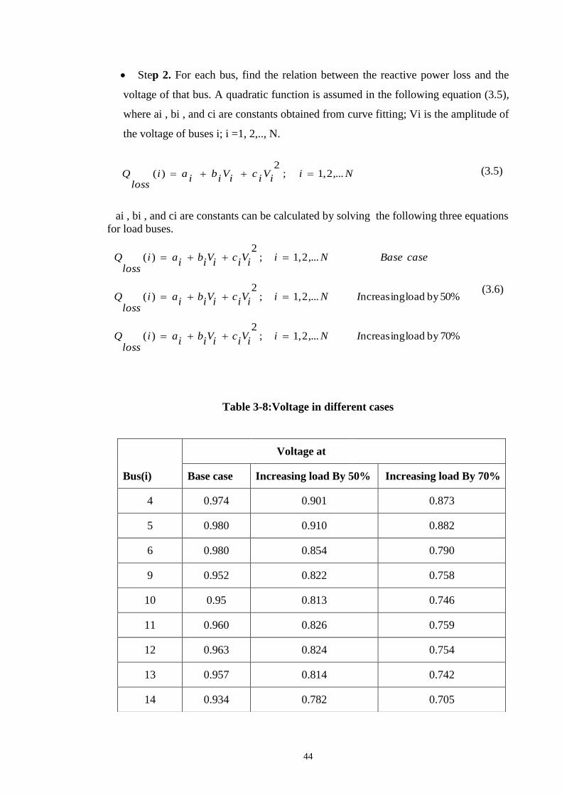
44
Step 2. For each bus, find the relation between the reactive power loss and the
voltage of that bus. A quadratic function is assumed in the following equation (3.5),
where ai , bi , and ci are constants obtained from curve fitting; Vi is the amplitude of
the voltage of buses i; i =1, 2,.., N.
,...2,1;2
)( Nii
Vi
ci
Vi
bi
ailoss
Q
(3.5)
ai , bi , and ci are constants can be calculated by solving the following three equations
for load buses.
70%by load ncreasing ,...2,1;2
)(
50%by load ncreasing ,...2,1;2
)(
,...2,1;2
)(
INii
Vi
ci
Vi
bi
ailoss
Q
INii
Vi
ci
Vi
bi
ailoss
Q
caseBaseNii
Vi
ci
Vi
bi
ailoss
Q
(3.6)
Table 3-8:Voltage in different cases
Voltage at
Bus(i) Base case Increasing load By 50% Increasing load By 70%
4 0.974 0.901 0.873
5 0.980 0.910 0.882
6 0.980 0.854 0.790
9 0.952 0.822 0.758
10 0.95 0.813 0.746
11 0.960 0.826 0.759
12 0.963 0.824 0.754
13 0.957 0.814 0.742
14 0.934 0.782 0.705

45
Table 3-9:Qlosses from load flow in different cases
Qlosees from load low
Bus(i) Base case Increasing load By 50% Increasing load By 70%
4 3.293 29.926 49.358
5 14.972 58.121 85.608
6 7.905 22.284 33.149
9 3.418 11.409 18.045
10 0.095 0.237 0.354
11 0.267 0.555 0.735
12 0.2 0.593 0.902
13 0.734 2.07 3.105
14 0.442 1.41 2.253
Table 3-10:Values of A,B and C.
Bus(i) A B C
4 3259.053 -6475.5605 3259.0533
5 3942.963 -7660.7969 3727.186589
6 364.8560 -651.254957 292.876723
9 232.23388 -447.5270 217.6199445
10 3.754515 -7.13865 3.458871
11 4.450025 -6.923591 2.673201
12 8.9479034 -16.39611 7.593050
13 27.908341 -50.795117 23.40624
14 20.99 -40.6856 19.998

46
3-11:Qlosses at base case and minimum voltage
Step 3. Derive the membership function of the reactive power losses from the
assumed membership function of the bus voltage using the above equation. Here, we
use a trapezoidal membership function for the bus voltage and the reactive power
losses. The formulation of these memberships is shown in “Figure3-3”.
Step 4. At a specific loading condition, determine, for each bus, the value of the
voltage membership and the value of reactive power loss membership as shown in
“Table3-12”.
Step 5. According to equation (3.4) ;multiply the two fuzzy sets to obtain the
decision S(i) for each bus. Arrange in an ascending order, for each loading condition
these decisions, from the smallest to the largest one. Buses having the smallest S are
specified as weak buses and we may need to install capacitor at these buses . “Table
3-13” shows that bus 14 is the weakest bus.
Bus(i) Qlosses at voltage
of base case
Qlosses at Vmin=0.95v
4 3.29299 8.21640
5 14.97199 28.9918
6 7.9050 10.485086
9 3.4179596 3.485224
10 0.09500 0.094429
11 0.26700 0.2851777
12 0.200 0.224317
13 0.73400 0.777115
14 0.4420 0.393860

47
Table 3-12: Voltage and reactive power losses membership
Table 3-13: Decision S(i) for each bus.
Bus(i) )(iuv )(iuq
4 1 1
5 1 1
6 1 1
9 1 1
10 1 1
11 1 1
12 1 1
13 1 1
14 0.9831 0.9976
Bus(i) Voltage(p.u) )(iuv )(iuq
)()()( iuiuiS qv
4 0.974 1 1 1
5 0.980 1 1 1
6 0.980 1 1 1
9 0.952 1 1 1
10 0.949 1 1 1
11 0.960 1 1 1
12 0.963 1 1 1
13 0.957 1 1 1
14 0.934 0.9831 0.9976 0.98074

48
C h a p t e r F o u r
4 SIMULATION OF ADOPTED SYSTEM.
4.1 CONTROL SYSTEM OF DSTATCOM
The use of compensators with improved qualifications such as distribution static
synchronous compensator (DSTATCOM) has garbed researcher's attention for
solving power quality problems. The (DSTATCOM) is a compensation device used
in a shunt configuration across the mains of the primary distribution system.
DSTATCOM makes use of a voltage source converter and internally generates
capacitive (i.e. leading) as well as inductive (i.e. lagging) reactive power. The
control system of the DSTATCOM is very fast and has the capability to provide
adequate reactive power compensation to the distribution system. Due to this
capability, DSTATCOM can be effectively used to regulate voltage drop that occurs
during the starting of large loads and/or large induction motors where the required
starting current is very high .Dstatcom is palced at bus 14 ;while thesize“Mvar”of
Dstatcom can be determined by using Bstatcom as shown in “(Figure 4-1)”.
Bstatcom is an ideal three phase voltage and current measurement, the size of
Dstatcom can change by changing the value of base power.
During switching Dstatcom to the system the current will be huge as well as
transient voltage as shown in “(Figure 4-2)”; low pass filter is used to reduce this
transient value so the transient voltage can be controlled as not exceed 1.05pu.To
calculate the consumed active and reactive power, single phase voltage and single
phase current are measured and these signals are connected to low pass filter to
reduce the transient. The filtered voltage and current signals are connected to fourier
analysis to give magnitude and angle. The product block takes three signals
(magnitude voltage, magnitude current and sin angle) to give the total consumed
reactive power.
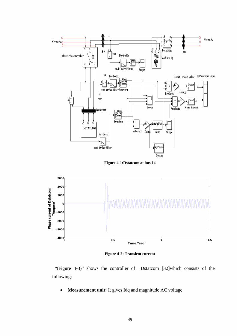
49
Figure 4-1:Dstatcom at bus 14
Figure 4-2: Transient current
“(Figure 4-3)” shows the controller of Dstatcom [32]which consists of the
following:
Measurement unit: It gives Idq and magnitude AC voltage
0 0.5 1 1.5-4000
-3000
-2000
-1000
0
1000
2000
3000
Time "sec"
Ph
ase c
urr
en
t o
f D
sta
tco
m
"Am
pere
"

50
AC voltage regulator: Compares between reference AC voltage and the
magnitude AC voltage to give (Iq ref).
DC voltage regulator: Compares between reference DC voltage and the
magnitude DC voltage to give (Id ref).
Mux: Has two inputs (Iq ref) and (Id ref) togiveoneoutput“Idq ref”.
Current regulator: Compares between (Idq ref) and the given (Idq) from the
measurement unit to give (Vdq) .
according to comparison between magnitude AC voltage and AC reference
voltage ;angle (phi) can be calculated from (Vdq) which used as a modulation
index for PWM
Figure 4-3: Controller of Dstatcom

51
“(Figure 4-4)” shows The voltage control system in ac voltage regulator of the
Dstatcom is adjusted to reference voltage and according to this value the reactive power
will conduct.
Figure 4-4: AC voltage regulator
4.2 SYSTEM VOLTAGE CONTROL USING DSTATCOM UNIT
To achieve the best results power quality and power reliability[33] are taken to
consideration by sizing Dstatcom according to network requirement and by placing
Dstatcom in more than one place according to the sensitivity of each bus respectively
.In this section, the effect of using Dstatcom unit to regulate the system voltage is
studied. The effect of changing the location as well as the size of the compensator unit
on the system voltage is conducted.
According to the sensitivity analysismethod∂Qi/∂|Viofbusno12comesnexttothatof
bus no 14. For this reason, bus no.12 and bus no.14 have been chosen to be the most
suitable locations for the compensator unit. “Table 3-5” has shown that 20MVAR
reactive compensator unit has been chosen for the rest of the analysis unless otherwise
stated, so the optimum size for Dsatacom will be 20MVAR for the following analysis.
4.2.1 Compensator located at bus 14
A 20MVAR compensator unit size is located at bus 14. The overall system dynamic
performance under different scenarios is studied. The voltage control system of the
Dstatcom shown in Figure 3-4 is adjusted such that to set the voltage at bus 14 to 1p.u.
or 0.98 pu..“(Figure4-5)”showstheeffectofswitchingonthecompensatorunitonthe

52
voltage at bus no.14. The compensator is switched on at t=0.4 sec. It is clear that the
Dstatcom unit injects the required capacitive reactive power to regulate the voltage at
the bus to thesetvalues.“(Figure4-6)” shows the instantaneous reactive power injected
by the voltage control unit under different values of the voltage reference set values.
Figure 4-5:Voltage at bus 14 when a 20MVAR Dstatcom unit is located at bus no.14
Figure 4-6:Injected reactive power at bus 14 when a 20MVAR Dstatcom unit is located at bus no.14
0.4 0.45 0.5 0.55 0.60.85
0.9
0.95
1
1.05
Time"sec"
Vo
ltag
e"p
u"
at
bu
s14
Dstatcom switching moment at bus 14
Set voltage ref=1pu
Set voltage ref=0.98pu
Without Dstatcom
0.4 0.45 0.5 0.55 0.6-4
-3
-2
-1
0
1x 10
7
Time"sec"
Reacti
ve p
ow
er"
Var"
Dstatcom switching moment
Set voltage ref=1pu
Set voltage ref=0.98pu

53
4.2.2 Compensator located at bus 12
The previous scenario is repeated when a 20MVAR compensator unit size is located at
bus 12 and the overall system performanceisinvestigated.“(Figure4-7)”and“(Figure
4-8)”showtheeffectofvoltagecontrolatbusno.12on the weakest bus voltage (bus
no.14) and on bus 12. The effect is clear in raising the bus voltage. The instantaneous
reactivepowerinjectedinthiscaseatbusno12isshownin“(Figure4-9)”.
Figure 4-7:Voltage at bus 14 when a 20MVAR Dstatcom unit is located at bus no.12
Figure 4-8:Voltage at bus 12 when a 20MVAR Dstatcom unit is located at bus no.12
0.4 0.45 0.5 0.55 0.60.9
0.92
0.94
0.96
0.98
1
1.02
Time"sec"
Vo
ltag
e"p
u"
at
bu
s14
Set voltage ref=0.98pu
Dstatcom switching moment at bus12
Set voltage ref=1pu
Without Dstatcom
0.4 0.45 0.5 0.55 0.6
0.9
0.95
1
1.05
1.1
Time"sec"
Vo
ltag
e"p
u"
at
bu
s12
Set voltage ref=1pu
Set voltage ref=0.98pu
Without DstatcomDstatcom switching moment at bus12
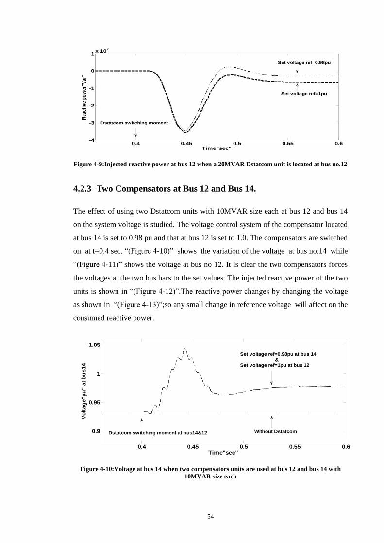
54
Figure 4-9:Injected reactive power at bus 12 when a 20MVAR Dstatcom unit is located at bus no.12
4.2.3 Two Compensators at Bus 12 and Bus 14.
The effect of using two Dstatcom units with 10MVAR size each at bus 12 and bus 14
on the system voltage is studied. The voltage control system of the compensator located
at bus 14 is set to 0.98 pu and that at bus 12 is set to 1.0. The compensators are switched
on at t=0.4 sec. “(Figure4-10)” shows the variation of the voltage at bus no.14 while
“(Figure4-11)” shows the voltage at bus no 12. It is clear the two compensators forces
the voltages at the two bus bars to the set values. The injected reactive power of the two
units is shown in “(Figure4-12)”.Thereactivepowerchangesby changing the voltage
as shown in “(Figure4-13)”;so any small change in reference voltage will affect on the
consumed reactive power.
Figure 4-10:Voltage at bus 14 when two compensators units are used at bus 12 and bus 14 with
10MVAR size each
0.4 0.45 0.5 0.55 0.6-4
-3
-2
-1
0
1x 10
7
Time"sec"
Rea
ctiv
e p
ow
er"V
ar"
Dstatcom switching moment
Set voltage ref=1pu
Set voltage ref=0.98pu
0.4 0.45 0.5 0.55 0.6
0.9
0.95
1
1.05
Time"sec"
Vo
ltag
e"p
u"
at
bu
s14
Without DstatcomDstatcom switching moment at bus14&12
Set voltage ref=0.98pu at bus 14
&
Set voltage ref=1pu at bus 12

55
Figure 4-11:Voltage at bus 12 when two compensators units are used at bus 12 and bus 14 with
10MVAR size each
Figure 4-12:Injected reactive power at bus 12 and 14 when two compensators units are used at bus
12 and bus 14 with 10MVAR size each
0.4 0.45 0.5 0.55 0.60.9
0.95
1
1.05
Time"sec"
Vo
ltag
e"p
u"
at
bu
s 1
2
Without Dstatcom
Set voltage ref=0.98pu at bus 14
&
Set voltage ref=1pu at bus 12
Dstatcom switching moment at bus14&12
0.4 0.45 0.5 0.55 0.6
-2
-1.5
-1
-0.5
0
0.5
1x 10
7
Time"sec"
Rea
ctiv
e p
ow
er"V
ar"
Dstatcom switching momentInst.raective power injected at bus 14
Q=-7.5MVAR
Inst.raective power injected at bus 12
Q=-1.75MVAR

56
Figure 4-13:Injected reactive power at bus 12 and 14 at different Vref
0.98 0.985 0.99 0.995 1 1.005 1.01 1.015 1.02 1.025 1.03-20
-15
-10
-5
0
Vref"pu"
Q "
MV
AR
"
Bus 14
Bus 12

57
4.3 RESPONSE OF DSTATCOM
This thesis shows how Dstacom supports the system during fault condition and when
reactive power loads increased where there is line outage that makes voltage-collapse,
this weakest line can be identify by using Fast Voltage Stability Index (FVSI).
4.3.1 Voltage Sag.
External short circuit can be represented by three phase fault on the transmission system
level as shown in “(Figure4-14)”whicheffect on distributed system“14bussystem”
by voltage sag.
Figure 4-14:Three phase fault on the transmission system level
The effect of the compensator size on the system in case of voltage sag is
investigated. A comparison between 20 MVAR and 100MVAR units(100MVAR is
unrealistic unit ;it used only for demonstrating the fault condition by using Dstatcom)
are undertaken. A voltage sag due to a three phase fault on the transmission system level
occurs at t=0.6 sec to t=0.9sec. “(Figure4-15)” shows that 20 MVAR compensator units
lightly improves the voltage at bus no 14 while the sag remains because of the limited

58
compensator size. Using a larger size compensator (100MVAR in this case), the voltage
at bus 14 is totally recovered. Yet, practically, using such large size compensator is not
economical. “(Figure4-16)”shows the required reactive compensation during the period
of the voltage sag in the two cases.
Figure 4-15:Voltage at bus 14 during fault
Figure 4-16: Consumed reactive power at bus 14 during fault
0.5 0.6 0.7 0.8 0.9 1 1.10.5
0.6
0.7
0.8
0.9
1
1.1
1.2
Time"sec"
Vo
ltag
e"p
u"
at
bu
s14
100 Mvar Dstatcom unit
20 Mvar Dstatcom unit
Without Dstatcom
Fault
0.5 0.6 0.7 0.8 0.9 1 1.1-12
-10
-8
-6
-4
-2
0
2
x 107
Time"sec"
Reacti
ve p
ow
er"
Var"
Inst.raective power injected out of 20 Mvar
Inst.raective power injected out of 100 Mvar

59
4.3.2 Line Outage
In case of IEEE 14 Bus system, line which connects bus 9 to bus 14 is considered to be
the critical line according to the fast voltage stability index (FVSI), by Taking the
symbols„i‟asthesendingbusand„j‟asthereceivingbus,FVSIiscalculated as shown
in “Table4-1”;where Qi ,Vi,X and Z are given in Appendix( A) and Appendix (B).In
this section line(14-9) is removed by switch as shown in“(Figure 4-17)” to simulate
contingency in the system and the dynamic response of the compensator unit located at
bus 14 is demonstrated. “(Figure 4-18)” shows the variation of the voltage at bus 14
with and without Dstatcom during line outage.. The compensator of 20 MVAR is
switched on at t=0.6 sec. As a result the compensator forces the voltage to recover to the
set reference value. The amount of reactive power needed corresponding to this case is
illustrated in “(Figure 4-19)”. At t=0.9 sec the line is reconnected to the system and the
compensator keeps the voltage at the set value.
Figure 4-17:System during line outage

60
Table 4-1:Fast voltage stability index
Bus line FVSI
4
2-4 -0.0290
3-4 -0.031401
5-4 -7.52*10-3
5
1-5 0.01344
2-5 0.011728
4-5 0.003
6
11-6 0.0763
12-6 0.10185
13-6 0.053674
9
10-9 0.071123
14-9 0.25128
4-9 Out
7-9 Out
10 9-10 0.0247
11-10 0.05717
11 6-11 0.018311
10-11 0.0181575
12 6-12 0.0209822
13-12 0.031030
13
6-13 0.0395
12-13 0.111
14-13 0.11488
14 13-14 0.094310
9-14 0.0728

61
Figure 4-18: Voltage at bus 14 during line outage
Figure 4-19: Consumed reactive power at bus 14 during line outage
0.3 0.4 0.5 0.6 0.7 0.8 0.9 1
0.85
0.9
0.95
1
1.05
1.1
Time"sec"
Vo
ltag
e"p
u"
at
bu
s14
Set voltage ref=1pu
Set voltage ref=0.98pu
Dstatcom switching moment at bus14
Without Dstatcom
Line"Back" Instant of Lineoutage
0.3 0.4 0.5 0.6 0.7 0.8 0.9 1
-5
-4
-3
-2
-1
0
1x 10
7
Time"sec"
Reacti
ve p
ow
er"
Var"
Set voltage ref=0.98pu
Set voltage ref=1pu
Line"Back"
Dstatcom switching moment
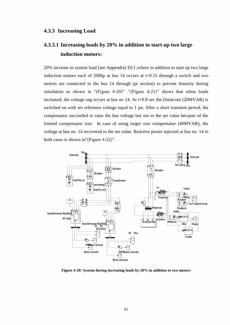
62
4.3.3 Increasing Load
4.3.3.1 Increasing loads by 20% in addition to start up two large
induction motors:
20% increase in system load [see Appendix( D) ] ;where in addition to start up two large
induction motors each of 200hp at bus 14 occurs at t=0.55 through a switch and two
motors are connected to the bus 14 through (pi section) to prevent linearity during
simulation as shown in “(Figure 4-20)” .“(Figure 4-21)” shows that when loads
increased, the voltage sag occurs at bus no 14. At t=0.8 sec the Dstatcom (20MVAR) is
switched on with set reference voltage equal to 1 pu. After a short transient period, the
compensator succeeded to raise the bus voltage but not to the set value because of the
limited compensator size. In case of using larger size compensator (40MVAR), the
voltage at bus no. 14 recovered to the set value. Reactive power injected at bus no. 14 in
bothcasesisshownin“(Figure4-22)”.
Figure 4-20: System during increasing loads by 20% in addition to two motors

63
Figure 4-21:Voltage at bus 14 in case of increasing the load
Figure 4-22:Injected reactive power at bus 14 in case of increasing the load
0.4 0.5 0.6 0.7 0.8 0.9 1 1.1 1.20.75
0.8
0.85
0.9
0.95
1
1.05
1.1
1.15
1.2
Time"sec"
Vo
ltag
e"p
u" a
t b
us14
Moment of increasing loads
Without Dstatcom
20 Mvar Dstatcom unit
40 Mvar Dstatcom unit
Dstatcom switching moment at bus14
0.4 0.5 0.6 0.7 0.8 0.9 1 1.1 1.2-10
-8
-6
-4
-2
0
x 107
Time"sec"
Reacti
ve p
ow
er"
Var"
Dstatcom switching moment
Inst.raective power
injected out of 20 Mvar
Inst.raective power
injected out of 40 Mvar
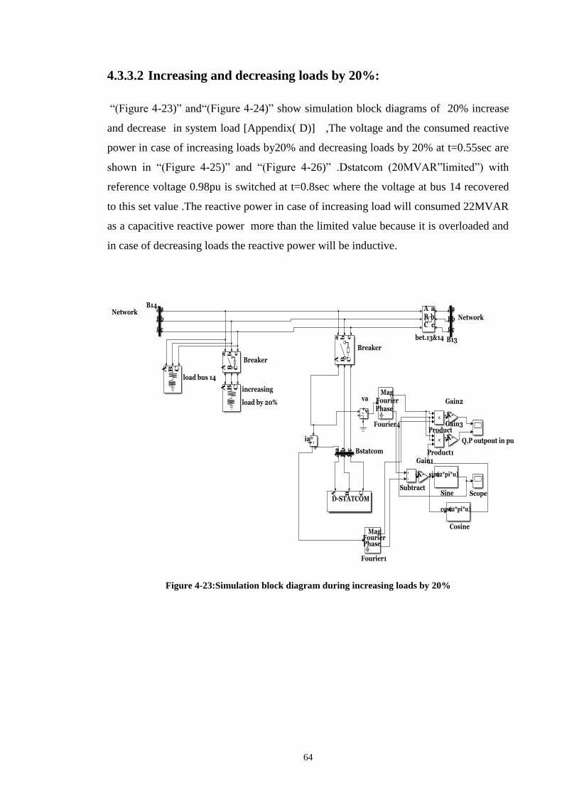
64
4.3.3.2 Increasing and decreasing loads by 20%:
“(Figure4-23)”and“(Figure4-24)”show simulation block diagrams of 20% increase
and decrease in system load [Appendix( D)] ,The voltage and the consumed reactive
power in case of increasing loads by20% and decreasing loads by 20% at t=0.55sec are
shown in “(Figure 4-25)” and “(Figure 4-26)” .Dstatcom (20MVAR”limited”) with
reference voltage 0.98pu is switched at t=0.8sec where the voltage at bus 14 recovered
to this set value .The reactive power in case of increasing load will consumed 22MVAR
as a capacitive reactive power more than the limited value because it is overloaded and
in case of decreasing loads the reactive power will be inductive.
Figure 4-23:Simulation block diagram during increasing loads by 20%

65
Figure 4-24: Simulation block diagram during decreasing loads by 20%
Figure 4-25:Voltage at bus 14 in case of increasing and decreasing loads by 20%
0.4 0.5 0.6 0.7 0.8 0.9 1 1.1 1.2
0.8
0.9
1
1.1
1.2
Time"sec"
Vo
ltag
e"p
u" a
t b
us14
Moment of switching loads
Increasing loads by 20%
Deecreasing loads by 20%
Dstatcom switching moment at bus14"Vref=0.98"
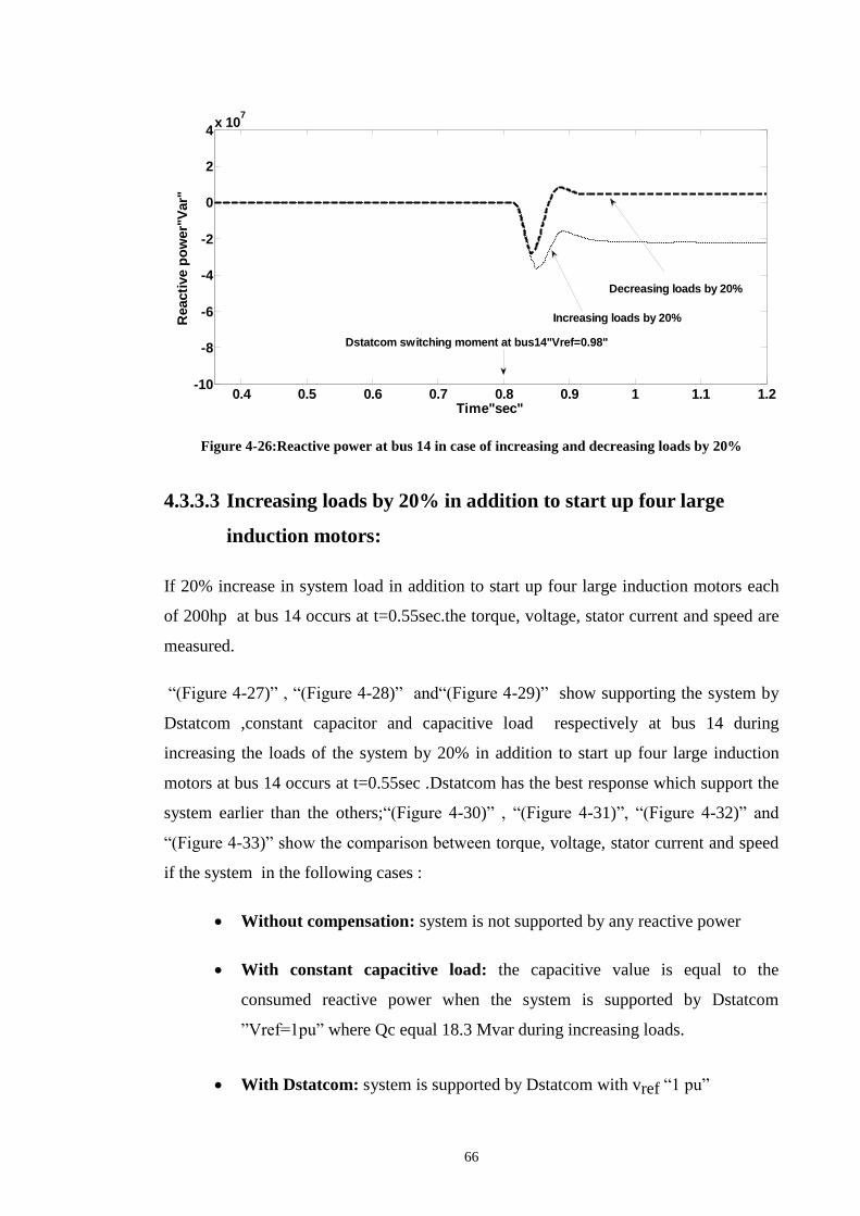
66
Figure 4-26:Reactive power at bus 14 in case of increasing and decreasing loads by 20%
4.3.3.3 Increasing loads by 20% in addition to start up four large
induction motors:
If 20% increase in system load in addition to start up four large induction motors each
of 200hp at bus 14 occurs at t=0.55sec.the torque, voltage, stator current and speed are
measured.
“(Figure4-27)”, “(Figure4-28)”and“(Figure4-29)” show supporting the system by
Dstatcom ,constant capacitor and capacitive load respectively at bus 14 during
increasing the loads of the system by 20% in addition to start up four large induction
motors at bus 14 occurs at t=0.55sec .Dstatcom has the best response which support the
system earlier than the others;“(Figure 4-30)” , “(Figure 4-31)”, “(Figure 4-32)” and
“(Figure4-33)”showthecomparisonbetween torque, voltage, stator current and speed
if the system in the following cases :
Without compensation: system is not supported by any reactive power
With constant capacitive load: the capacitive value is equal to the
consumed reactive power when the system is supported by Dstatcom
”Vref=1pu” where Qc equal 18.3 Mvar during increasing loads.
With Dstatcom: system is supported by Dstatcom with vref “1pu”
0.4 0.5 0.6 0.7 0.8 0.9 1 1.1 1.2-10
-8
-6
-4
-2
0
2
4x 10
7
Time"sec"
Reacti
ve p
ow
er"
Var"
Increasing loads by 20%
Decreasing loads by 20%
Dstatcom switching moment at bus14"Vref=0.98"

67
With constant capacitor: : by trial the capacitive value to give 1 pu at bus
14 where the capacitance value is equal to (3*10-4
).
Figure 4-27: IEEE 14 bus system supported by Dstatcom during increasing loads by 20% in
addition to four motors
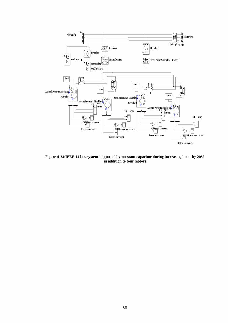
68
Figure 4-28:IEEE 14 bus system supported by constant capacitor during increasing loads by 20%
in addition to four motors

69
Figure 4-29: IEEE 14 bus system supported by capacitive load during increasing loads by 20% in
addition to four motors

70
Figure 4-30: Speed of induction motors when system is supported by different types of
compensation
Figure 4-31:Stator current of induction motors when system is supported by different types of
compensation
0 0.5 1 1.5 2 2.5 3 3.5
0
100
200
Without compensator
0 0.5 1 1.5 2 2.5 3 3.5
0
100
200
Sp
eed
With capacitive load
0 0.5 1 1.5 2 2.5 3 3.5
0
100
200
With Dstatcom
0 0.5 1 1.5 2 2.5 3 3.5
0
100
200
Time"sec"
With constant capacitor
0 0.5 1 1.5 2 2.5 3 3.5-2
0
2x 10
4
Without compensator
0 0.5 1 1.5 2 2.5 3 3.5-2
0
2x 10
4
Sta
tor C
urren
t
With capacitive load
0 0.5 1 1.5 2 2.5 3 3.5-2
0
2x 10
4
With Dstatcom
0 0.5 1 1.5 2 2.5 3 3.5-2
0
2x 10
4
Time"sec"
With constant capacitor

71
Figure 4-32:Torque of induction motors when system is supported by different types of
compensation
Figure 4-33:Voltage at bus 14 when system is supported by different types of compensation
0 0.5 1 1.5 2 2.5 3 3.5-2000
0
2000
Without compensator
0 0.5 1 1.5 2 2.5 3 3.5-2000
0
2000
To
rq
ue
With capacitive load
0 0.5 1 1.5 2 2.5 3 3.5-2000
0
2000
With Dstatcom
0 0.5 1 1.5 2 2.5 3 3.5-2000
0
2000
Time"sec"
With constant capacitor
0.5 1 1.5 2 2.5 3 3.50.9
0.95
1
Without compensation
0.5 1 1.5 2 2.5 3 3.50.9
0.95
1
Vo
ltag
e a
t b
us 1
4
With capacitive load
0.5 1 1.5 2 2.5 3 3.50.9
0.95
1
With Dstatcom
0.5 1 1.5 2 2.5 3 3.50.9
0.95
1
Time"sec"
With constant cap
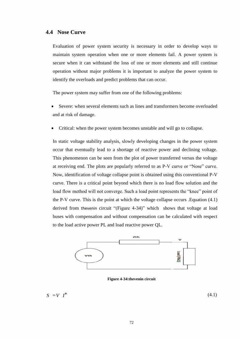
72
4.4 Nose Curve
Evaluation of power system security is necessary in order to develop ways to
maintain system operation when one or more elements fail. A power system is
secure when it can withstand the loss of one or more elements and still continue
operation without major problems it is important to analyze the power system to
identify the overloads and predict problems that can occur.
The power system may suffer from one of the following problems:
Severe: when several elements such as lines and transformers become overloaded
and at risk of damage.
Critical: when the power system becomes unstable and will go to collapse.
In static voltage stability analysis, slowly developing changes in the power system
occur that eventually lead to a shortage of reactive power and declining voltage.
This phenomenon can be seen from the plot of power transferred versus the voltage
at receiving end. The plots are popularly referred to as P-Vcurveor“Nose”curve.
Now, identification of voltage collapse point is obtained using this conventional P-V
curve. There is a critical point beyond which there is no load flow solution and the
loadflowmethodwillnotconverge.Suchaloadpointrepresentsthe“knee”pointof
the P-V curve. This is the point at which the voltage collapse occurs .Equation (4.1)
derived from thevenin circuit “(Figure 4-34)” which shows that voltage at load
buses with compensation and without compensation can be calculated with respect
to the load active power PL and load reactive power QL.
Figure 4-34:thevenin circuit
IVS
(4.1)

73
0
V
QjP
V
SI
(4.2)
thZIVthV th
(4.3)
)()0
( thXthRV
QjPVthV th
(4.4)
2)(2)(V
thQR
V
thPX
V
thQX
V
thPRVV th (4.5)
2
22
2
22
2
22
2
222422
222(
V
RQ
V
XP
V
XQ
V
RPQXVPRVV thththth
ththV thV
(4.6)
)(22(( 2222
24
)0 QpQXPRVVththhh ZVtt
(4.7)
22223
222
1
34
4222
222
12
2
LQ
ThZP
ThZK
ThPEThRPthRthXLQK
PthRthXLQK
KThELQ
ThEThX
ThX
LQKP
ThRKThE
LVV
(4.8)
Where:
Eth: thevenin voltage.
Zth: Total thevenin impedance.
Xth: thevenin line reactance .
Rth: thevenin resistance.

74
V : load voltage.P:Active power.
QL:load reactive power.
“(Figure4-35)”and“(Figure4-36)”showhowOpencircuitvoltage“Eth” and short
circuit current at bus 12 and bus 14.Eth and Isc can be calculated by putting three
phase fault and by removing the load at the required bus and replaced by a constant
value of a capacitive load as shown in “Table4-2” ,so the required Zth can be
calculated in“Table4-3” and “Table4-4” . “(Figure4-37)” and“(Figure3-38)”
show the total nose curve in different cases by coding equation(4.1) in matlab as
shown in Appendix (C).
Figure 4-37)”and“(Figure3-38)”indicatethat load active power bus 14 reach zero
faster than bus 12 which indicates that bus 14 is the weakest bus.
Table 4-2:Average voltage and standard deviation
Dstatcom
location (MVAR)
Vref (p.u.) Injected Qc
(MVAR)
Bus 14 Bus 12 Bus 14 Bus 12 Bus
14
Bus12
20 - 0.99 - 10.65 0
- 20 - 0.99 0 5
10 10 0.98 1 7.5 1.75
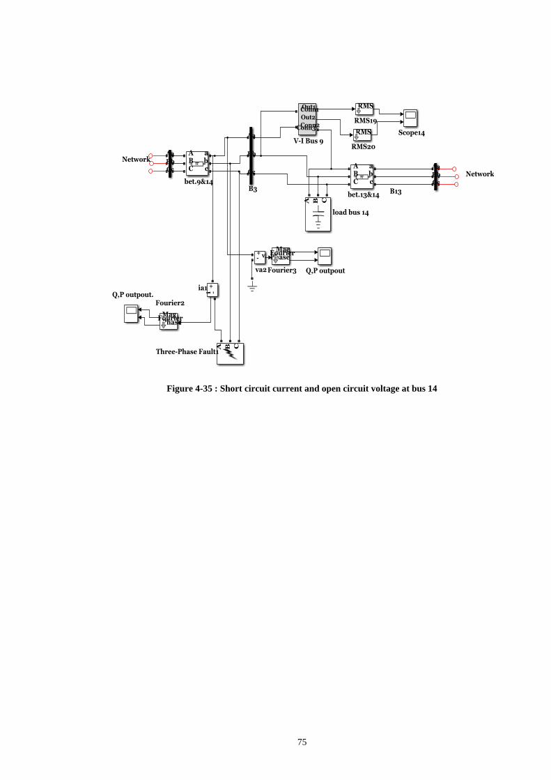
75
Figure 4-35 : Short circuit current and open circuit voltage at bus 14

76
Figure 4-36: Short circuit current and open circuit voltage at bus 12
Table 4-3: Eth, Rth, Xth and Isc calculations at bus 14
Dsatacom
location(MVAR)
Vref of Dstatcom) Eth (pu) Isc (pu) Rth (pu) Xth (pu)
Without
compensation
- 0.99293 2.366 0.165725 0.38855
10MVAR at bus14
&
10MVAR at bus12
0.98pu at bus14
&
1pu at bus 12 1.034554 2.41454 0.163276 0.396138
20MVAR at bus
14
0.99pu at bus14 1.043340 2.412346 0.165510 0.39957

77
Table 4-4:Eth, Rth, Xth and Isc calculations at bus 12
Dsatacom
location(MVAR)
Vref of
Dstatcom
Eth (pu) Isc (pu) Rth (pu) Xth (pu)
Without
compensation
- 0.9864 2.2 0.177 0.412
10MVAR at bus14
&
10MVAR at bus12
0.98pu at bus14
&
1pu at bus 12 1.004645 2.239 0.17712 0.41226
20MVAR at bus 12 0.99pu at bus12 1.013432 2.2069 0.182885 0.42120
Figure 4-37:Nose cure at bus 14
0 1 2 3 4 5 6
0.6
0.65
0.7
0.75
0.8
0.85
0.9
0.95
1
1.05
Pload
Vo
ltag
e"p
u" a
t b
us14
Without compensation
Dstatcom at Bus14(Vref=0.99pu)
Dstatcom at Bus14(Vref=0.98pu)
and Bus 12(Vref=1pu)

78
Figure 4-38: Nose cure at bus 12
0 2 4 6 8 10 12 14 16
0.6
0.65
0.7
0.75
0.8
0.85
0.9
0.95
1
1.05
Pload
Vo
ltag
e"p
u" a
t b
us12
Without compensation
Dstatcom at Bus12(Vref=0.99pu)
Dstatcom at Bus14(Vref=0.98pu)
and Bus12 (Vref=1pu)

79
C h a p t e r F i v e
5 RESULTS.
5.1 SYSTEM VOLTAGE CONTROL USING DSTATCOM UNIT
5.1.1 Compensator located at bus 14:
A 20MVAR compensator unit size is located at bus 14. The overall system dynamic
performance under different scenarios is studied. “Table 5-1” shows that by
changing the voltage reference value from 0.98 to 1 pu change the required reactive
power from -8.7 MVAR to -12.7MVAR ; the reference voltage affects on the total
system average voltage and standard deviation; this table demonstrates that the
average voltage during each case are semi equal , but the reference voltage affects
on the consumed reactive power and standard deviation
Chapter 4 demonstrates bus 14 is the best location for Dstatcom. If Dstatcom is
placed in load buses such as bus 6,9,10,11,12,13 and 14 to enforce the voltage at bus
14 to be 1 pu “13800 volt” by regulating the reference voltage in AC voltage
regulator for each bus; the consumed reactive power will be calculated in each case
as shown in “Table 5-2”which demonstrates that bus 14 consumes the minimum
reactive power.
Table 5-1:Average voltage and standard deviation when Dstatcom is located at bus 14
Bus Vref (pu) Vavg (pu) S.D (σ) Q(Mvar)
14 1 1.011232 0.02138 -12.7
0.98 1.0008585 0.02420 -8.7

80
Table 5-2:Injected Qc to approach 1pu at bus 14
Bus
Vref
6 9 10 11 12 13 14
1.06 20 VAR 18.8Mvar
1.021 23.5MVAR
1.028 19.5Mvar
1.05 20Mvar
1.04 18.2Mvar
1 12.7Mvar
5.1.2 Compensator located at bus 12:
The previous scenario is repeated when a 20MVAR compensator unit size is located
at bus 12 and the overall system performanceisinvestigated.“Table5-3”showsthat
by changing the voltage reference value from 0.98 to 1 pu change the required
reactive power from -3 MVAR to -6.75MVAR. The reference voltage affects on the
total system average voltage and standard deviation, this table demonstrates that the
bus 14 is the best location for Dsatacom by comparing average voltage and standard
deviation when Dsatacom is placed at bus 14 and bus 12.
Table 5-3:Average voltage and standard deviation when Dstatcom is located at bus 12
Bus Vref (pu) Vavg (pu) S.D (σ) Q(Mvar)
12 1 0.99438 0.02561 -6.75
0.98 0.981936 0.02405 -3
5.1.3 Two Compensators at Bus 12 and Bus 14.
A20MVAR compensator unit size is located at bus 12 & bus14.“Table5-4” shows
the sizing of Dstatcom which depends on reference voltage where The best one is
0.98 pu at bus 14 and 1 pu at bus 12 which consume a capacitive MVAR as well as
MVAR will be inductive if the reference voltage is 1 pu at bus 14 and 0.98 pu at
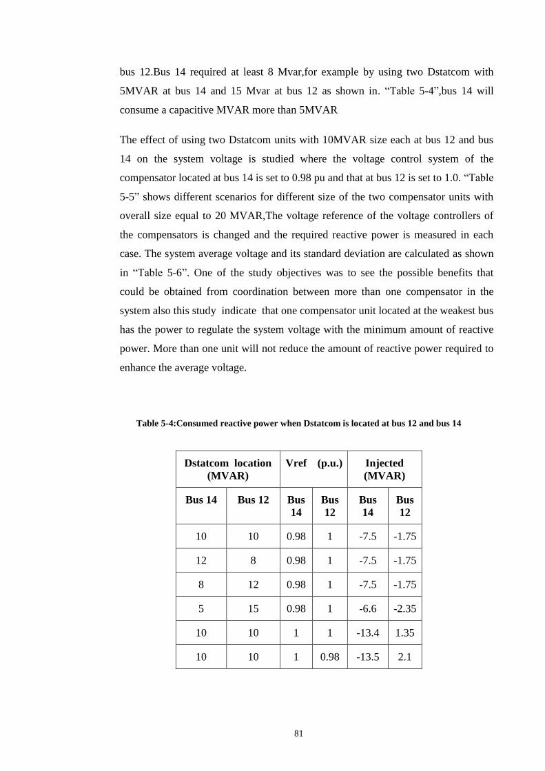
81
bus 12.Bus 14 required at least 8 Mvar,for example by using two Dstatcom with
5MVAR at bus 14 and 15 Mvar at bus 12 as shown in. “Table 5-4”,bus 14 will
consume a capacitive MVAR more than 5MVAR
The effect of using two Dstatcom units with 10MVAR size each at bus 12 and bus
14 on the system voltage is studied where the voltage control system of the
compensator located at bus 14 is set to 0.98 pu and that at bus 12 is set to 1.0. “Table
5-5” shows different scenarios for different size of the two compensator units with
overall size equal to 20 MVAR,The voltage reference of the voltage controllers of
the compensators is changed and the required reactive power is measured in each
case. The system average voltage and its standard deviation are calculated as shown
in “Table 5-6”. One of the study objectives was to see the possible benefits that
could be obtained from coordination between more than one compensator in the
system also this study indicate that one compensator unit located at the weakest bus
has the power to regulate the system voltage with the minimum amount of reactive
power. More than one unit will not reduce the amount of reactive power required to
enhance the average voltage.
Table 5-4:Consumed reactive power when Dstatcom is located at bus 12 and bus 14
Dstatcom location
(MVAR)
Vref (p.u.) Injected
(MVAR)
Bus 14 Bus 12 Bus
14
Bus
12
Bus
14
Bus
12
10 10 0.98 1 -7.5 -1.75
12 8 0.98 1 -7.5 -1.75
8 12 0.98 1 -7.5 -1.75
5 15 0.98 1 -6.6 -2.35
10 10 1 1 -13.4 1.35
10 10 1 0.98 -13.5 2.1

82
Table 5-5:Total consumed reactive power
Dstatcom
location (MVAR)
Vref (p.u.) InjectedQc MVAR Voltage in pu
Bus 14 Bus 12 Bus
14
Bus 12 Bus 14 Bus 12 Bus
14
Bus 12
20 - 0.98 - 8.7 0 0.98 0.995
- 20 - 0.995 0 6 0.955 0.995
- 20 - 1.01 0 8.8 0.964 1.01
- 20 - 1.02 0 10.7 0.978 1.02
- 20 - 1.033 0 13.2 0.98 1.033
10 10 0.98 0.995 8.75 0 0.98 0.995
10 10 0.98 1.01 5.2 5.2 0.98 1.01
10 10 0.98 1.02 3 8.6 0.98 1.02
10 10 0.98 1.033 0 13.4 0.98 1.033
Table 5-6: Total Average voltage and standard deviation
Dstatcom
location
(MVAR)
Vref
(p.u.)
Vavrg
in
pu
ST.D
in
pu
Bus 14 Bus 12 Bus 14 Bus 12
20 - 0.98 - 1.0008 0.0242
- 20 - 0.995 0.9918 0.0278
- 20 - 1.01 0.9996 0.0265
- 20 - 1.02 1.0050 0.0255
- 20 - 1.033 1.0122 0.0251
10 10 0.98 0.995 1.0008 0.0244
10 10 0.98 1.01 1.0052 0.0238
10 10 0.98 1.02 1.0080 0.0242
10 10 0.98 1.033 1.0113 0.0243

83
5.2 RESPONSE OF DSTATCOM
5.2.1 Voltage sag
20 MVAR and 100 MVAR compensator are used at bus no 14 during sag while, 20
MVAR compensator units lightly improves the voltage at bus no 14 while the sag
remains because of the limited compensator size.Using a larger size compensator
(100MVAR in this case), the voltage at bus 14 is totally recovered ;using such large size
compensator is not economical but it used to demonstrate that during fault the system
consumed a large amount of reactive power to recover the system voltage as shown in
“Table5-7”.
Table 5-7: Consumed reactive power and voltage without compensation at bus 14 during fault
Bus Size of Dstatcom
(MVAR)
Voltage at bus 14
(pu)
Q(Mvar)
100 0.97 -100
14 20 0.7 -20
5.2.2 Line outage
The compensator of 20 MVAR is used during line outage. the reference voltage
affects on the total system average voltage and standard deviation as well as the
consumedreactivepowerasshownin“Table5-8”and“Table5-9”.
;

84
Table 5-8:Total consumed reactive power during line outage
Dstatcom location
(MVAR)
Vref (p.u.) Injected (MVAR)
Bus 14 Bus 12 Bus
14
Bus
12
Bus 14 Bus 12
10 10 0.98 1 -9.3 -8*10-5
10 10 1 0.98 -13.2 5.3
20 - 0.98 - -10 -
20 - 1 - -12 -
- 20 - 0.98 - -5.7
- 20 - 1 - -7.6
Table 5-9:Average voltage and standard deviation during line outage
Dstatcom
location
(MVAR)
Vref
(p.u.)
Vavrg
in
pu
ST.D
in
pu
Bus 14 Bus 12 Bus 14 Bus 12
10 10 0.98 1 0.998190 0.02449
10 10 1 0.98 0.99024635 0.026142
20 - 0.98 - 0.996068 0.02500
20 - 1 - 1.002350 0.024532
- 20 - 0.98 0.98220 0.0326
- 20 - 1 0.98652 0.031634
- - - - 0.9682 0.040055

85
5.2.3 Increasing load
When system loads increased by 20% in addition to two motors ;Dstatcom (20MVAR)
is switched to the system with set reference voltage equal to 1 pu the compensator
succeeded to raise the bus voltage but not to the set value because of the limited
compensator size. In case of using larger size compensator (40MVAR), the voltage at
bus no. 14 recovered to the set value. According to the reference voltage of the
compensator the consumed reactive power will be injected .“Table 5-10” shows the
total consumed reactive power in both cases and the voltage at bus 14 before and after
compensation. This table indicates that during increasing static and dynamic loads the
system needs more reactive power ;so the system should be supported by (31MVAR)
capacitive reactive power as well as the limited reactive power (20MVAR) is not
suitable for this case
Table 5-10:Total consumed reactive power during increasing loads by 20% in addition to two
motors
Bus Vref
pu
Size of Dstatcom
MVAR
Voltage at bus
14 (pu) before
compensation
Voltage at bus
14 (pu) after
compensation
Qconsumed
(Mvar)
40 0.87 1 -31
14 1 20 0.87 0.944 -20
Without Dstatcom 0.934 - -
If system loads (static loads only) increased by 20% and decreased by 20% ;Dstatcom
(20MVAR) is switched to the system with set reference voltage equal to 0.98 pu the
compensator succeeded to raise the bus voltage to this set value. The total consumed
reactive power in case of increasing loads will be 22MVAR as a capacitive reactive
power more than the set value because the system is overloaded and the voltage will
change from 0.9 pu to 0.98 pu ( setvaue“0.98pu”) ; but in case of decreasing loads the
consumed reactive power will be inductive as the system is enforced to be in the set
value“0.98pu”.“Table5-11”showsThetotalconsumedreactivepowerthevoltageat
bus 14 in each case and the voltage at bus 14 before and after compensation

86
Table 5-11:Total consumed reactive power during increasing and decreasing loads by 20%
Bus Vref
0.98
pu
Size of
Dstatcom
MVAR
Voltage at bus 14
(pu) before
compensation
Voltage at bus 14
(pu) after
compensation
Qconsumed
(Mvar)
Dec. 20 0.997 0.98 0.5*10-7
14 Inc. 20 0.9 0.98 -22

87
C h a p t e r S i x
6 CONCLUSION.
In this work, several methods have been utilized to identify the weakest busbar in an
IEEE 14 bus system. The potential benefits that can be derived by applications of
Dstatcom to industrial facility have been investigated. A study specifying the location as
well as the suitable size of the Dstatcom unit that enhances the system voltage profile
has been undertaken.. The study revealed that a small change in the reference voltage
leads to a large change in the required reactive compensation. Locating the voltage
compensator unit at the weakest bus will enhance the system average voltage.
One of the study objectives was to see the possible benefits that could be obtained from
coordination between more than one compensator in the system indicated that one
compensator unit located at the weakest bus has the power to regulate the system
voltage with the minimum amount of reactive power. A trial has been made to see if
using more than one compensator can help enhancing voltage regulation and decreasing
the required reactive power, More than one unit will not reduce the amount of reactive
power required to enhance the average voltage.The study indicated that the best results
are obtained by locating one compensator with proper size at the weakest bus. The
results indicated also the capability of the Dstatcom with proper size to counteract
voltage sag ,increasing loads and/or line outage.
Dstatcom has a good response which reduce time to interact with any power system,
and it can be used with static and dynamic loads; so it can be used in industrial work
.this thesis shows economical results by using Dstatcom in different cases and the
reference voltage can control the amount of the consumed reactive power

88
REFERENCES
[1] Bresestietal,“Powersystemplanningunderuncertaintyconditions.Criteriafor
transmission network flexibility evaluation,” IEEE Bologna power Tech.
conference June 23th-26th Bologna Italy, 2003.
[2] Aydogan Ozdemir and Chanan Singh, “Fuzzy logic based mw contingency
ranking againstmasking problem,” Power Engineering SocietyWinterMeeting
IEEE, Vol. 2, pp 504-509, 2001.
[3] Shahidehpouretal,“Impactofsecurityonpowersystemsoperation,”Proceedings
of the IEEE, Vol. 93, No. 11, pp 2013-2025,November 2005 178.
[4] N.Farokhnia, S.H. Fathi,R.Khoraminia, S.H.Hosseinian, “Optimization of PI
Coefficients in DSTATCOMNonlinear Controller for Regulating DC Voltage
usingGeneticAlgorithm”, ICIEA Conference 2009, pp 2291-2296.
[5] D.K.Rai, H.K Verma, L.S.Titare:‟Maximum permissible loading of a power
system withinvoltage stability limits usingThevenin parameters IJERA vol 2 issue
4 july-aug. 2012 pp 2172-2176
[6] G. F. Ledwich, S. H. Hosseini and G. F. Shannon, “VoltageBalancing using
SwitchedCapacitors”,JournalofElectricPowerSystemResearch,Vol.24,1992,
pp. 85-90.
[7] G. Reed, M.Takeda, F.Ojima, A.Sidell, R. Chervus and C.Nebecker,"Application
of 5 MVA, 4.16kV DSTATCOM for Voltage Flicker atSeattle Iron and Metals,"
Proceedings of IEEE PES Summer Meeting, 2000, Vol. 3, p 1605-1611.
[8] H.Akagi, Y.Kanazawa and A.Nabae, "Instantaneous Reactive Compensators
Comprising Switching Devices without Energy Storage Components,"
IEEETransactions on Industry Applications, Vol. IA-20, No. 3, 1984, pp. 625-
630.

89
[9] B.N.Singh, K.Al-Haddad and A.Chandra, "DSP based Indirect-current Controlled
STATCOM -I Multifunctional Capabilities" IEE Proceedings,Vol. 147, No. 2,
March 2000, pp. 107-112.
[10] B.N.Singh, K.Al-Haddad, A.Chandra, "DSP based Indirect-current Controlled
STATCOM - II Multifunctional capabilities," IEE Proceedings,Vol. 147, No. 2,
March 2000, pp. 13-118.
[11] O. Lara and E. Acha, "Modeling and Analysis of Custom Power Systems
byPSCAD/ EMTDC," IEEE Transactions on Power Delivery, Vol. 17,No.1,2002,
pp. 266-272.
[12] T. J.E.Miller, “ReactivePowerControl inElectricSystems”,Toronto,Canada:
Wiley, 1982.
[13] A.Ghosh and G. Ledwich, “Power Quality Enhancement using CustomPower
Devices”,KluwerAcademicPublishers,London2002.
[14] D.P.Kothari and I.J.Nagrath, "Electric Machines," Tata McGraw Hill, India, 2004.
[15] J.B Gupta,B.Sc (Electrical Engineering); C.Eng.(I) ;F.I.E.(India) ;M.I.S.T.E. ,
Power System(Generation and Economic Considerations, Transmission and
Distribution,Switchgear and Protection),published by Sanjeev Kumar
Kataria,Ninth Edition – March 2002,Re-Print 2004,chapter 18.
[16] William D.Stevenson,Jr, Elements Of Power System Analysis, 4th Edition,
chapter14.
[17] Leonard L. Grigsby, Electric Power Engineering Handbook (Power System
Stability and Control), by Taylor & Francis Group, LLC ,Second Edition, 2006,
chapter 7.
[18] Emad-Eldin Abdel-Khalek Dabbis, "Effect of FACTS devices on power system
voltage stability", PHD thesis, Faculty of Engeneering ,Cario universty
Giza,Egypt,June 2007 .

90
[19] Ahmed Mostafa Mahammed Mahammed,"Improving the voltage stability of
electrical power systems using shunt FACTS devices", mastar thesis, Faculty of
eEngeneering ,Cario universty Giza, Egypt, June 2009.
[20] Sami Repo,"On-Line Voltage Stability Assessment Of Power System An-
Approach Of Black-box Modeling ", PHD thesis, Tampere university of
technology and the academy, Finland 2001.
[21] P.P.Deo,B.Sc.(Engg.),M.Tech(I.I.T),M.S(Binghamton,USA),M.I.E.Consultant
Engineer Pune, Power System Analysis & Stability, published dy Technical
Publications Pune, First Edition: April 2005, chapter13.
[22] ] BelkacemMahdad1,TarekBouktir ,KamelSrairi1 “StrategyofLocationand
Control of FACTS Devices for Enhancing Power Quality”, IEEE MELECON
2006, May 16-19, Benalmadena (Malaga), Spain, pp1068-1072.
[23] Priyanko Guha Thakurta, “An Approach for Optimal Placement of SVC to
Minimize Load Curtailment” , Master Thesis, Electrical Power System, Royal
Institute of Technology-KTH, Stockholm, Sweden, May 2009.
[24] A. M. El-Zonkoly,"Optimal Sizing of SSSC Controllers to Minimize
Transmission Loss and a Novel Model of SSSC to Study Transient Response",
World Academy of Science, Engineering and Technology , 2006, pp5-11.
[25] Hadi Saadat,"Power System Analysis", TATA McGRAWHILL,2004.
[26] Timothy J. Ross, FUZZY LOGIC WITH ENGINEERING APPLICATIONS,
Second Edition, John Wiley & Sons Ltd, The Atrium, Southern Gate, Chichester,
West Sussex PO19 8SQ, England, 2004.
[27] S. N. Sivanandam, S. Sumathi and S. N. Deepa, Introduction to Fuzzy Logic using
MATLAB, Springer Berlin Heidelberg New York,2007.
[28] Didier Dubois and Henri Prade, Fuzzy Sets and Systems: Theory and
Applications, ACADEMIC PRESS, INC,1980.
91
[29] I.Musirin,T.K.A.Rahman“NovelFastVoltageStabilityIndex(FVSI)forVoltage
Stability Analysis in Power TransmissionSystem”2002StudentConference on
Research and Development Proceedings, ShahAlam, Malaysia, July 2002.
[30] A. Chakraborti, D.P. Kothari, A.K. Mukhopadhyay, A. De,“Anintroduction to
Reactive Power Control and Voltage Stabilityin Power Transmission Systems”,
1st edition, Prentice HallIndia, 2010
[31] Simulation Method to Identify the Weakest Bus and ItsVoltage Stability Margin
in a Multi-bus Power Network”,Proceeding of International Conference MS‟07,
India,December 3-5,2007, pp. 1-5.
[32] Yao Xu”Adaptive PI Control of STATCOM for Voltage Regulation”, IEEE
Transactions on Power Delivery ,Vol:29 , Issue: 3 , 14 February 2014.
[33] Y. Ansari1, M.Gaidhane, K.Sawalakhe “Stabilization of Voltage in Power System
by Using STATCOM”, International Journal on Recent and Innovation Trends in
Computing and Communication, Volume: 3 Issue: 2, February 2015
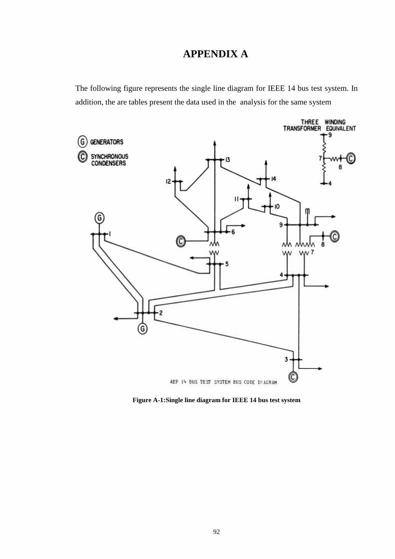
92
APPENDIX A
The following figure represents the single line diagram for IEEE 14 bus test system. In
addition, the are tables present the data used in the analysis for the same system
Figure A-1:Single line diagram for IEEE 14 bus test system

93
Table A-1:Line data-IEEE 14 bus system
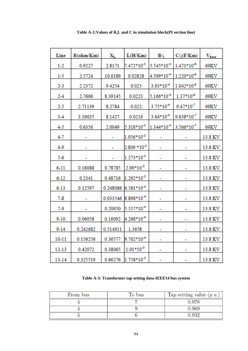
94
Table A-2:Values of R,L and C in simulation block(PI section line)
Table A-3: Transformer tap setting data-IEEE14 bus system

95
Table A-4:Shunt capacitor data-IEEE 14 bus system
Table A-5:Bus data-IEEE 14 bus system

96
APPENDIX B
Table B-1:Load flow-14 Bus System
Power Flow Solution by Newton-Raphson Method
Maximum Power Mismatch = 0.000126875
No. of Iterations = 6
Bus Voltage Angle ------Load------ ---Generation--- Injected
No. Mag. Degree MW Mvar MW Mvar Mvar
1 1.060 0.000 0.000 0.000 233.913 36.693 0.000
2 1.025 -4.795 21.700 12.700 40.000 33.038 0.000
3 0.990 -13.026 94.200 19.100 0.000 38.860 0.000
4 0.974 -10.060 47.800 -3.900 0.000 0.000 0.000
5 0.980 -8.494 7.600 1.600 0.000 0.000 0.000
6 0.980 -14.808 11.200 7.500 0.000 0.000 0.000
7 0.966 -13.511 0.000 0.000 0.000 0.000 0.000
8 0.966 -13.511 0.000 0.000 0.000 0.000 0.000
9 0.952 -15.410 29.500 16.600 0.000 0.000 0.000
10 0.949 -15.645 9.000 5.800 0.000 0.000 0.000
11 0.960 -15.374 3.500 1.800 0.000 0.000 0.000

97
12 0.963 -15.833 6.100 1.600 0.000 0.000 0.000
13 0.957 -15.907 13.800 5.800 0.000 0.000 0.000
14 0.934 -16.849 14.900 5.000 0.000 0.000 0.000
Total 259.300 73.600 273.913 108.590 0.000
Line Flow and Losses
--Line-- Power at bus & line flow --Line loss-- Transformer
from to MW Mvar MVA MW Mvar tap
1 233.913 36.693 236.773
2 159.071 14.060 159.691 4.414 7.738
5 74.860 22.631 78.206 2.998 7.811
2 18.300 20.338 27.359
1 -154.657 -6.323 154.786 4.414 7.738
3 74.727 3.700 74.818 2.512 6.785
4 56.337 10.627 57.330 1.852 0.699
5 41.893 12.345 43.674 1.060 -0.183

98
3 -94.200 19.760 96.250
2 -72.215 3.085 72.281 2.512 6.785
4 -21.985 16.677 27.595 0.561 -1.906
4 -47.800 3.900 47.959
2 -54.485 -9.928 55.382 1.852 0.699
3 22.546 -18.583 29.218 0.561 -1.906
5 -59.620 6.764 60.003 0.507 0.378
7 27.711 15.181 31.597 0.000 2.103 0.978
9 16.048 10.465 19.159 0.000 2.019 0.969
5 -7.600 -1.600 7.767
1 -71.862 -14.820 73.375 2.998 7.811
2 -40.834 -12.528 42.712 1.060 -0.183
4 60.128 -6.386 60.466 0.507 0.378
6 44.968 32.133 55.269 0.000 6.966 0.932
6 -11.200 -7.500 13.479
5 -44.968 -25.168 51.532 0.000 6.966
11 7.609 6.150 9.783 0.095 0.198
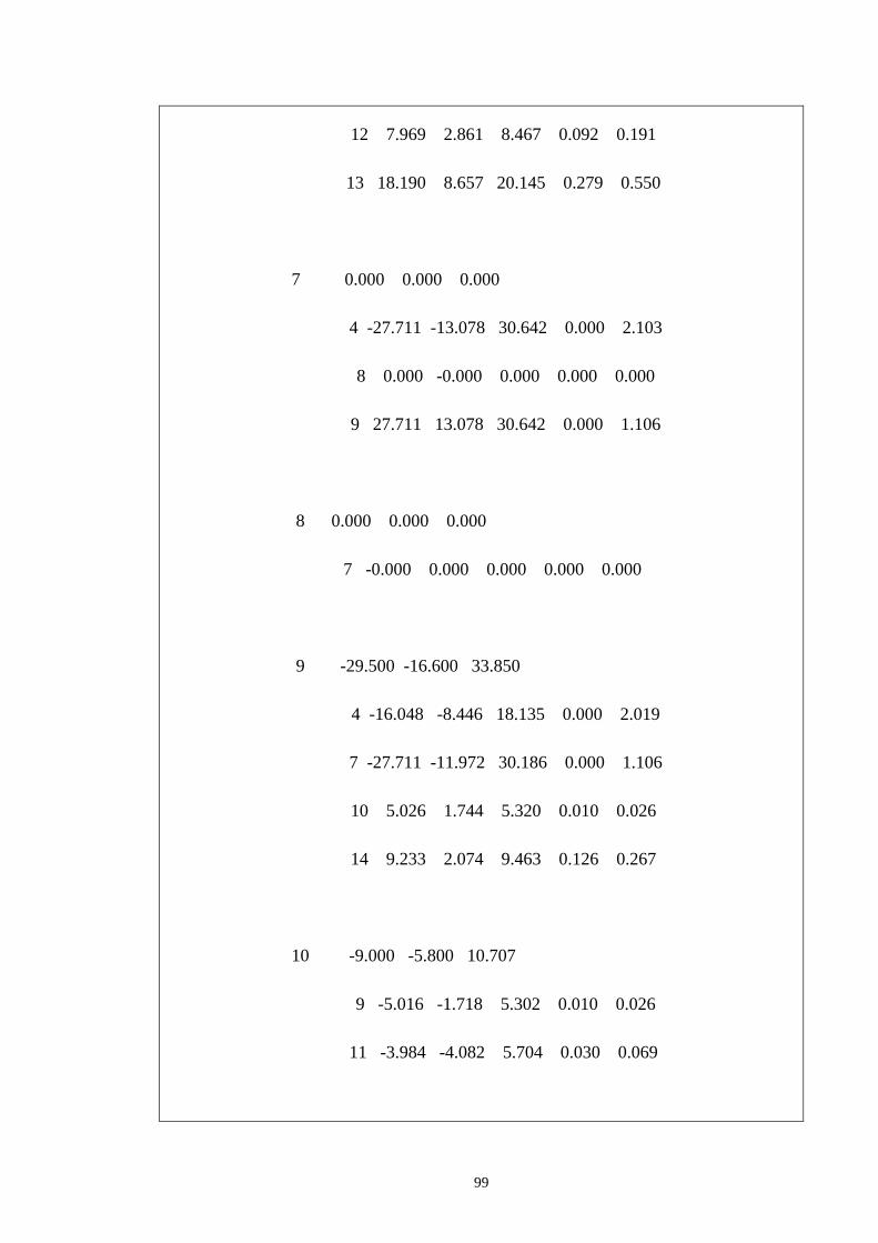
99
12 7.969 2.861 8.467 0.092 0.191
13 18.190 8.657 20.145 0.279 0.550
7 0.000 0.000 0.000
4 -27.711 -13.078 30.642 0.000 2.103
8 0.000 -0.000 0.000 0.000 0.000
9 27.711 13.078 30.642 0.000 1.106
8 0.000 0.000 0.000
7 -0.000 0.000 0.000 0.000 0.000
9 -29.500 -16.600 33.850
4 -16.048 -8.446 18.135 0.000 2.019
7 -27.711 -11.972 30.186 0.000 1.106
10 5.026 1.744 5.320 0.010 0.026
14 9.233 2.074 9.463 0.126 0.267
10 -9.000 -5.800 10.707
9 -5.016 -1.718 5.302 0.010 0.026
11 -3.984 -4.082 5.704 0.030 0.069

100
11 -3.500 -1.800 3.936
6 -7.514 -5.952 9.586 0.095 0.198
10 4.014 4.152 5.775 0.030 0.069
12 -6.100 -1.600 6.306
6 -7.878 -2.670 8.318 0.092 0.191
13 1.778 1.070 2.075 0.010 0.009
13 -13.800 -5.800 14.969
6 -17.911 -8.107 19.660 0.279 0.550
12 -1.767 -1.061 2.061 0.010 0.009
14 5.878 3.367 6.775 0.086 0.175
14 -14.900 -5.000 15.717
9 -9.107 -1.807 9.285 0.126 0.267
13 -5.793 -3.193 6.614 0.086 0.175
Total loss 14.631 35.002

101
Table B-2:Y Bus
Y b
us
:Colu
mns
1 t
hro
ugh 5
:
6.0
250
-1
9.4
98
1i
-
4.9
99
1 +
15.2
63
1i
0
0
-
1.0
259
+ 4
.23
50
i
-4.9
99
1 +
15
.26
31
i
9.5
213
-3
0.3
54
7i
-1
.135
0 +
4.7
819
i
-1.6
860
+ 5
.11
58
i
-1
.70
11
+ 5
.193
9i
0
-1
.13
50 +
4.7
819
i
3
.121
0 -
9.8
50
7i
-
1.9
86
0 +
5.0
68
8i
0
0
-1.6
860
+ 5
.11
58
i
-1.9
86
0 +
5.0
68
8i
10
.513
0 -
38
.34
31i
-6
.84
10
+2
1.5
78
6i
-1.0
25
9 +
4.2
35
0i
-1
.701
1 +
5.1
93
9i
0
-6.8
410
+2
1.5
78
6i
9.5
68
0 -
34
.97
54
i
0
0
0
0
0
+ 3
.96
79
i
0
0
0
0
+ 4
.7819
i
0
0
0
0
0
0
0
0
0
0
+ 1
.7980
i
0
0
0
0
0
0
0
0
0
0
0
0
0
0
0
0
0
0
0
0
0
0
0
0
0
0
Y b
us
:Colu
mns
6 t
hro
ugh
10 :
0
0
0
0
0
0
0
0
0
0
0
0
0
0
0
0
0
+ 4
.781
9i
0
0 +
1.7
98
0i
0
0 +
3.9
679
i
0
0
0
0
6.5
79
9 -
17
.34
07
i
0
0
0
0
0
0
-19
.54
90
i
0 +
5.6
770
i
0
+ 9
.09
01
i
0
0
0 +
5.6
77
0i
0
- 5
.67
70
i
0
0
0
0
+ 9
.09
01
i
0
5
.32
61 -
24
.282
5i
-3
.902
0 +
10
.36
54
i
0
0
0
-3.9
02
0 +
10
.36
54
i
5
.782
9 -
14
.76
83
i
-1
.95
50
+ 4
.09
41
i
0
0
0
-1
.880
9 +
4.4
02
9i
-1.5
26
0 +
3.1
76
0i
0
0
0
0
-3.0
98
9 +
6.1
02
8i
0
0
0
0
0
0
0
-1
.42
40 +
3.0
291
i
0
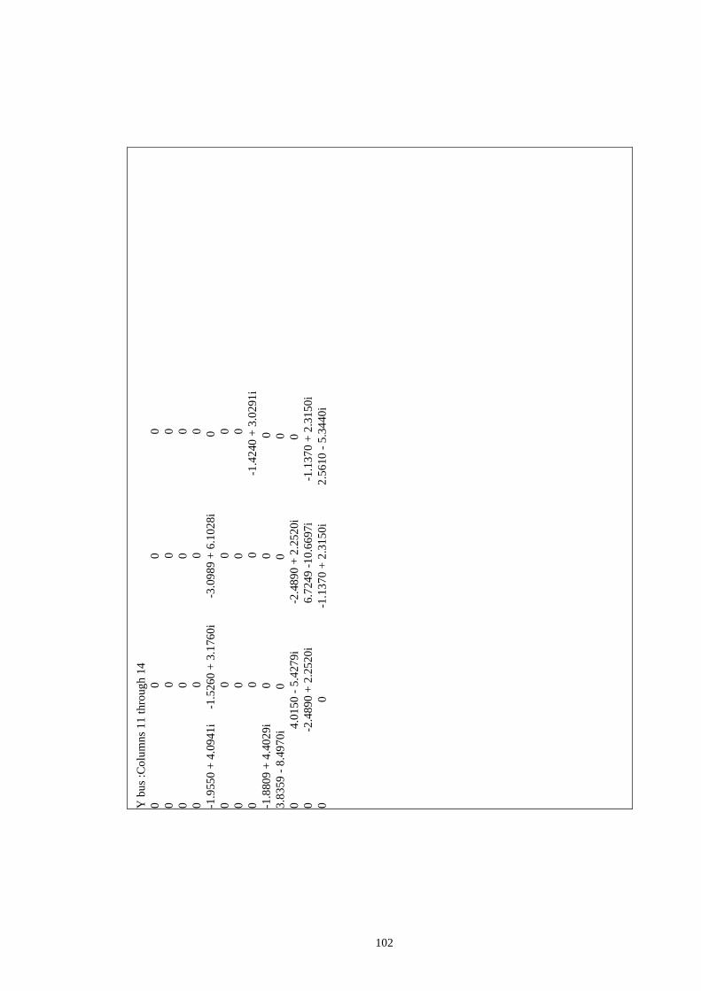
102
Y
bu
s :C
olu
mn
s 1
1 t
hro
ug
h 1
4
0
0
0
0
0
0
0
0
0
0
0
0
0
0
0
0
-1.9
55
0 +
4.0
94
1i
-1.5
26
0 +
3.1
76
0i
-3
.09
89 +
6.1
02
8i
0
0
0
0
0
0
0
0
0
0
0
0
-1
.42
40
+ 3
.02
91
i
-1.8
80
9 +
4.4
02
9i
0
0
0
3.8
359
- 8
.49
70
i
0
0
0
0
4
.01
50
- 5
.427
9i
-2
.48
90
+ 2
.25
20i
0
0
-2
.48
90 +
2.2
52
0i
6
.724
9 -
10
.66
97i
-1
.13
70
+ 2
.31
50
i
0
0
-1.1
37
0 +
2.3
15
0i
2.5
610
- 5
.34
40
i

103
APPENDIX C
Table C-1: Without compensation-Nose curve for bus 12
A=0.486492;
Q=0.016;
x=0.412;
R=0.177;
RD=0.03133;
vD=0.973;
QD=0.000256;
xD=0.1697;
B=0.23667;
zD=0.2;
PLp=[0:0.001:0.769];
vp=sqrt((A-Q.*x-R.*PLp + sqrt(RD.*PLp.^2+2.*PLp.*R.*x.*Q-
R.*vD.*PLp+QD.*xD-Q.*x.*vD+B-zD.*PLp.^2-zD.*QD)));
PLn=[0.769:-0.001:0];
vn=sqrt((A-Q.*x-R.*PLn - sqrt(RD.*PLn.^2+2.*PLn.*R.*x.*Q-
R.*vD.*PLn+QD.*xD-Q.*x.*vD+B-zD.*PLn.^2-zD.*QD)));
PL=[PLp PLn];
v2=[vp vn];
plot(PL*16.4,v2)
Table C-2:Vref"0.99pu” at bus 12-Nose curve for bus 12
A=0.513522;
Q=0.016;
x=0.42120;
R=0.182885;
RD=0.0334469;
vD=1.0270444;
QD=0.000256;
xD=0.177409;
B=0.2637050;
zD=0.2108646;
PLp=[0:0.001:0.79];
vp=sqrt((A-Q.*x-R.*PLp + sqrt(RD.*PLp.^2+2.*PLp.*R.*x.*Q-
R.*vD.*PLp+QD.*xD-Q.*x.*vD+B-zD.*PLp.^2-zD.*QD)));
PLn=[0.79:-0.001:0];
vn=sqrt((A-Q.*x-R.*PLn - sqrt(RD.*PLn.^2+2.*PLn.*R.*x.*Q-
R.*vD.*PLn+QD.*xD-Q.*x.*vD+B-zD.*PLn.^2-zD.*QD)));
PL=[PLp PLn];
v2=[vp vn];
plot(PL*16.4,v2)
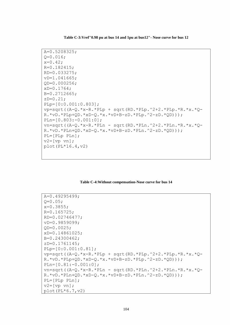
104
Table C-3:Vref"0.98 pu at bus 14 and 1pu at bus12"- Nose curve for bus 12
A=0.5208325;
Q=0.016;
x=0.42;
R=0.182415;
RD=0.033275;
vD=1.041665;
QD=0.000256;
xD=0.1764;
B=0.2712665;
zD=0.21;
PLp=[0:0.001:0.803];
vp=sqrt((A-Q.*x-R.*PLp + sqrt(RD.*PLp.^2+2.*PLp.*R.*x.*Q-
R.*vD.*PLp+QD.*xD-Q.*x.*vD+B-zD.*PLp.^2-zD.*QD)));
PLn=[0.803:-0.001:0];
vn=sqrt((A-Q.*x-R.*PLn - sqrt(RD.*PLn.^2+2.*PLn.*R.*x.*Q-
R.*vD.*PLn+QD.*xD-Q.*x.*vD+B-zD.*PLn.^2-zD.*QD)));
PL=[PLp PLn];
v2=[vp vn];
plot(PL*16.4,v2)
Table C-4:Without compensation-Nose curve for bus 14
A=0.49295499;
Q=0.05;
x=0.3855;
R=0.165725;
RD=0.02746477;
vD=0.9859099;
QD=0.0025;
xD=0.14861025;
B=0.24300462;
zD=0.1761145;
PLp=[0:0.001:0.81];
vp=sqrt((A-Q.*x-R.*PLp + sqrt(RD.*PLp.^2+2.*PLp.*R.*x.*Q-
R.*vD.*PLp+QD.*xD-Q.*x.*vD+B-zD.*PLp.^2-zD.*QD)));
PLn=[0.81:-0.001:0];
vn=sqrt((A-Q.*x-R.*PLn - sqrt(RD.*PLn.^2+2.*PLn.*R.*x.*Q-
R.*vD.*PLn+QD.*xD-Q.*x.*vD+B-zD.*PLn.^2-zD.*QD)));
PL=[PLp PLn];
v2=[vp vn];
plot(PL*6.7,v2)

105
Table C-5:Vref"0.99pu” at bus 12-Nose curve for bus 14
A=0.544279177;
Q=0.05;
x=0.39957;
R=0.165510;
RD=0.0273935;
vD=1.08855;
QD=0.0025;
xD=0.159656;
B=0.296239;
zD=0.187056;
PLp=[0:0.001:0.875];
vp=sqrt((A-Q.*x-R.*PLp + sqrt(RD.*PLp.^2+2.*PLp.*R.*x.*Q-
R.*vD.*PLp+QD.*xD-Q.*x.*vD+B-zD.*PLp.^2-zD.*QD)));
PLn=[0.875:-0.001:0];
vn=sqrt((A-Q.*x-R.*PLn - sqrt(RD.*PLn.^2+2.*PLn.*R.*x.*Q-
R.*vD.*PLn+QD.*xD-Q.*x.*vD+B-zD.*PLn.^2-zD.*QD)));
PL=[PLp PLn];
v2=[vp vn];
plot(PL*6.7,v2)
Table C-6:Vref"0.98 pu at bus 14 and 1pu at bus12"- Nose curve for bus 14
A=0.5351514033;
Q=0.05;
x=0.396138;
R=0.163276;
RD=0.0266590;
vD=1.0703028;
QD=0.0025;
xD=0.1569253;
B=0.2863870244;
zD=0.1835848;
PLp=[0:0.001:0.87];
vp=sqrt((A-Q.*x-R.*PLp + sqrt(RD.*PLp.^2+2.*PLp.*R.*x.*Q-
R.*vD.*PLp+QD.*xD-Q.*x.*vD+B-zD.*PLp.^2-zD.*QD)));
PLn=[0.87:-0.001:0];
vn=sqrt((A-Q.*x-R.*PLn - sqrt(RD.*PLn.^2+2.*PLn.*R.*x.*Q-
R.*vD.*PLn+QD.*xD-Q.*x.*vD+B-zD.*PLn.^2-zD.*QD)));
PL=[PLp PLn];
v2=[vp vn];
plot(PL*6.7,v2)
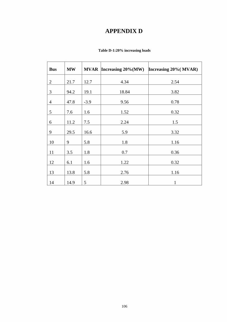
106
APPENDIX D
Table D-1:20% increasing loads
Bus MW MVAR Increasing 20%(MW) Increasing 20%( MVAR)
2 21.7 12.7 4.34 2.54
3 94.2 19.1 18.84 3.82
4 47.8 -3.9 9.56 0.78
5 7.6 1.6 1.52 0.32
6 11.2 7.5 2.24 1.5
9 29.5 16.6 5.9 3.32
10 9 5.8 1.8 1.16
11 3.5 1.8 0.7 0.36
12 6.1 1.6 1.22 0.32
13 13.8 5.8 2.76 1.16
14 14.9 5 2.98 1
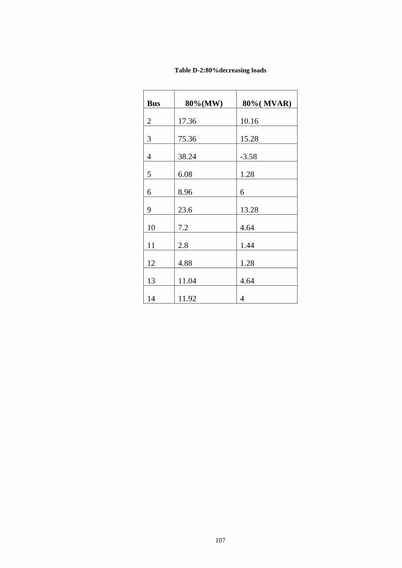
107
Table D-2:80%decreasing loads
Bus 80%(MW) 80%( MVAR)
2 17.36 10.16
3 75.36 15.28
4 38.24 -3.58
5 6.08 1.28
6 8.96 6
9 23.6 13.28
10 7.2 4.64
11 2.8 1.44
12 4.88 1.28
13 11.04 4.64
14 11.92 4

108
يهخص انرسانت
عي حغش اىدذ ف شبنت (DSTATCOM)ح بسث اىخأثش اىخاص بإضافت اىاص الاعخاحن
زث ح دساعت إخخاس اىغعت اىاعبت .حصع مشباء حسخ عي اسبعت عشش قضب حصو
مزىل إعخخذا ف خخيف اىاقع عي اىشبنت ىخسغ (DSTATCOM)ىياص الاعخاحن
.اىدذ بشبنت اىخصع اىنشبت
ف داه شبناث اىخصع (DSTATCOM)زا اىبسث شمض عي حطبقاث اىاص الاعخاحن
ح حعذو اىرج اىخفصي اىخاص باىاص .اثاء حغش الازاه عاءا اىذانت ا اىثابخت
أخو اىصه لأفضو أداء دان ى لإصلاذ حثبج اىدذ (DSTATCOM)الاعخاحن
زث ح دساعت اىدذ أثاء عياث اىغيق اىفخر ىلأزاه .بدع قضبا اىخصو باىشبنت
.اىصاعت اىنبشة خشج ازذ خطط اىخصع زالاث بط اىدذ
بأام خخيفت ع (DSTATCOM)إعخعشض اىبسث إعخخذا ععاث خخيفت ىياص الاعخاحن
.الأخز ف الاعخباس اىسفاظ عي أقو إعخلاك ىيطاقت اىغش فعاىت
ف . ك69) قطب حصو 14ز اىذساعت ح حسققا إثباحا عي ظا حصع قاع ن
.بذ إضافت ا سغاث ىيدذ (ف. ك13.8/
عي حغش خذ (DSTATCOM)اىخائح حشش إى اىخأثش اىاضر لأعخخذا اىاص الاعخاحن
ح عشض حسغ .اىظا أثاء زالاث اىخشغو اىطبعت ما ف اىسالاث الاخش اىغش طبعت
.أداء اىشبنت خدت ىيخعذلاث اىخسغاث اىخ حج إضافا

109
الأكادييت انعربيت نهعهىو وانتكىنىجيا وانقم انبحري
كهيت انهذست وانتكىنىجيا
قسى هذست انكهرباء وانتحكى
,
الاداء انذياييكي نهىاز الاستاتيكي نعانجت حالاث
تغير انجهذ في ظاو انتىزيع انكهربي
اخغخش سعاىت
ف
ذعت اىنشباء اىخسن
قذت
يي سرور إبراهيى / انهذست
اىنشباء اىخسنبناىسط ذعت
رايا يتىني انشرقاوي. / د.أ
يشرف __________________________________
رزق حىدة. / د. أ
يشرف ________________________________
ياسر جلال. / د.أ
يتح __________________________________
ابراهيى هلال. / د.أ
يتح __________________________________

110
الأكادييت انعربيت نهعهىو وانتكىنىجيا وانقم انبحري
كهيت انهذست وانتكىنىجيا
قسى هذست انكهرباء وانتحكى
,
الاداء انذياييكي نهىاز الاستاتيكي نعانجت حالاث
تغير انجهذ في ظاو انتىزيع انكهربي
اخغخش سعاىت
ف
ذعت اىنشباء اىخسن
قذت
يي سرور إبراهيى / انهذست
اىنشباء اىخسنبناىسط ذعت
حسج إششاف
رايا يتىني انشرقاوي. / د.أ رزق حىدة. / د. أ قغ ذعت اىنشباء اىخسنسئظ
الأمادت اىعشبت ىيعي اىخنىخا
اىقو اىبسش
قغ ذعت اىنشباء اىخسن سئظ
ذعت ع شظ
2016