Dynamic quantile linear models: a Bayesianapproach

Kelly C. M. GoncalvesIM-UFRJ

Helio S. MigonIM-UFRJ

Leonardo S. BastosPROCC-Fiocruz

Abstract

A new class of models, named dynamic quantile linear models, ispresented. It combines dynamic linear models with distribution freequantile regression producing a robust statistical method. Bayesianinference for dynamic quantile linear models can be performedusing an efficient Markov chain Monte Carlo algorithm. A fastsequential procedure suited for high-dimensional predictive modelingapplications with massive data, in which the generating process is itselfchanging overtime, is also proposed. The proposed model is evaluatedusing synthetic and well-known time series data. The model is alsoapplied to predict annual incidence of tuberculosis in Rio de Janeirostate for future years and compared with global strategy targets setby the World Health Organization.

This paper aims to combine two innovative areas developed during the lastquarter of the twentieth century building a useful broad new class of models,namely dynamic linear models and quantile regression. In the 1970s somenew ideas to model time series data were put forward by Jeff Harrison and co-authors (Harrison and Stevens 1976). This class of models can be ingeniouslyviewed as regression models with parameters varying throughout time. Atalmost the same time, Roger Koenker introduced the quantile regressionmodels, generalizing the L1 regression, a robust procedure that has since beensuccessfully applied to a range of statistical models (Koenker and Bassett1978). It provides richer information on the effects of the predictors than doesthe traditional mean regression and it is very insensitive to heteroscedasticityand outliers, accommodating the non-normal errors often encountered inpractical applications.

1

The inferential approaches of dynamic linear models and quantileregression are, nevertheless, completely distinct. While the first contributionfollows the Bayesian paradigm, the other resorts to optimization techniquesto solve the stated minimization problem, and its inference is theoreticallyfounded on large sample theory. In the next paragraphs, we state the mainnovelties in both consolidated areas.

A simple minimization problem yielding the ordinary sample quantiles inthe location model was shown to generalize naturally to the linear model,generating a broad new class of models introduced in the 1970s by Koenkerand Bassett (1978) named “quantile regression models”. Bayesian inferencefor quantile regression proceeds by forming the likelihood function basedon the asymmetric Laplace distribution (Yu and Moyeed 2001). The recentliterature includes a large number of papers: Yue and Rue (2011) add randomeffects to account for over-dispersion caused by unobserved heterogeneityor for correlation in longitudinal data; Luo et al. (2012) discuss inferenceusing MCMC methods for longitudinal data models with random effects;Alhamzawi et al. (2011) discuss prior elicitation; Peng et al. (2014) explorevarying covariate effects, including a new perspective on variable selection;Yang et al. (2016) evaluate the asymptotic validity of posterior inference; Yu(2015) presents quantile regression method for hierarchical linear models.

Quantile regression is also applied to temporal and spatially referenceddata as a flexible and interpretable method of simultaneously detectingchanges in several features of the distribution of some variables. A methodbased on estimating the conditional distribution was given by Cai (2002)and quantile autoregression was introduced by Koenker and Xiao (2006).Moreover, Reich et al. (2011) and Reich (2012) developed, respectively, aspatial and a spatiotemporal quantile regression models and, Reich and Smith(2013) proposed a semi-parametric quantile regression model for censoredsurvival data. Applications of quantile regression have become widespreadin recent years: in finance, actuarial modelign (Taylor 1999; Bassett Jrand Chen 2002; Kudryavtsev 2009; Sriram et al. 2016); in public policiesevaluation (Neelon et al. 2015; Rahman 2016); in residual lifetime (Li et al.2016).

Dynamic linear models (DLM) were introduced by Harrison and Stevens(1976) and extended to generalized linear models by West et al. (1985). TheDLM are part of a broad class of models with time varying parameters,useful for modeling and forecasting time series and regression data (West andHarrison 1997; Durbin and Koopman 2002; Migon et al. 2005; Petris et al.2009; Prado and West 2010). The advent of stochastic simulation techniquesstimulated applications of the state space methodology to model complexstochastic structures, like dynamic spatiotemporal models (Gamerman et al.

2

2003), dynamic survival models (Bastos and Gamerman 2006), dynamiclatent factor models (Lopes et al. 2008), and multiscale modeling (Ferreiraet al. 2011; Fonseca and Ferreira 2017). Real applications of the methodologyhas been also appeared in hydrology (Ravines et al. 2008; Fernandes et al.2009), intraday electricity load (Migon and Alves 2013), finance (Zhao et al.2016), and many other areas.

We extend the dynamic linear models to a new class, named dynamicquantile linear models, where a linear function of the state parameters is setequal to a quantile of the response variable at time t, yt, similar to the quantileregression of Koenker (2005). This method is suited for high-dimensionalpredictive modeling applications with massive data in which the generatingprocess itself changes over time. Our proposal keeps the most relevantcharacteristics of DLM such as: (i) all relevant information sources are used:history, factual or subjective experiences, including knowledge of forthcomingevents; (ii) everyday forecasting is generated by a statistical model andexceptions can be taken into account as an anticipative or retrospective base;(iii) what happened and what if analysis are easily accommodated; and (iv) themodel can be decomposed into independent components describing particularfeatures of the process under study.

The relative ease with which Markov chain Monte Carlo (MCMC)methods can be used to obtain the posterior distributions, even in complexsituations, has made Bayesian inference very useful and attractive, however,at the expense of losing the sequential analysis of both states andparameters. Therefore, some fast computing alternatives exploring analyticalapproximations are welcome, as in Da-Silva et al. (2011) and Souza et al.(2018). In this paper, we introduce the inference via MCMC methods, andalso via an alternative approach based on normal approximations and Bayeslinear estimation (West et al. 1985), which besides being computationallyfaster than MCMC, recovers the sequential analysis of the data. Ourapproximation procedure provides the marginal likelihood sequentially asnew data arrive, which is essential to perform sequential model monitoringand model selection (West 1981).

The remainder of the paper is organized as follows. Section 2 exploresin more details the dynamic quantile linear model. Section 3 presents ourefficient MCMC algorithm and the sequential approach for the dynamicquantile linear modeling. Section 4 illustrates the proposed method withsynthetic data, and also presents some results of the well-known time seriesof the annual flow of the Nile River at Aswan from 1871 to 1970. The modelis also applied to time series data on tuberculosis in Rio de Janeiro state,Brazil, from 2001 to 2015. We also predict the incidence for future years andcompare the results with those of the global tuberculosis strategy targets

3

established. Finally, Section 5 concludes with discussion of the paper andsome possible extensions.

1 Dynamic quantile linear model

The τ -th quantile of a random variable yt at time t can be represented as alinear combination of explanatory variables,

Qτ (yt) = F′tθ(τ)t ,

where Qτ (yt) is the τ -quantile of yt, formally defined as Qτ (yt) = inf{y∗ :P (yt < y∗) ≥ τ}, for 0 < τ < 1. Ft is a p× 1 vector of explanatory variables

at time t, and θ(τ)t is a p×1 vector of coefficients depending on τ and t. From

now on, the superscript τ will be omitted in order to keep the notation assimple as possible.

For a given time t, Koenker and Bassett (1978) defined the τ -th quantileregression estimator of θt as any solution of the quantile minimizationproblem

minθt

ρτ (yt − F′tθt) ,

where ρτ (.) is the loss (or check) function defined by ρτ (u) = u(τ−I(u < 0)),with I(·) denoting the indicator function. Minimizing the loss function ρτ (·)is equivalent to maximizing the likelihood function of an asymmetric Laplace(AL) distribution, as pointed out by Yu and Moyeed (2001). However,instead of maximizing the likelihood, as Yu and Moyeed (2001), we derivethe posterior distribution of the τ -th quantile regression coefficients at timet using the AL. Therefore, regardless the distribution of yt, it is enough toassume that:

yt | µt, φ, τ ∼ AL(µt, φ

−1/2, τ), t = 1, 2, . . . , T, (1)

where µt = F′tθt ∈ R is a location parameter, φ−1/2 > 0 is a scale parameter,and τ ∈ (0, 1) is a skewness parameter representing the quantile of interest.In dynamic modeling, one goal is also to obtain the predictive distribution.This can be done in a robust fashion using a grid of values of τ ∈ (0, 1) todescribe the full predictive distribution of yt. Nevertheless, in this paper, wefocus on providing precise inference about the linear predictor µt for eachτ -th quantile.

In a dynamic linear model, the states at time t depend on the states attime t− 1 according to an evolution equation θt = Gtθt−1 +wt, where Gt isa (p× p) matrix describing the evolution parameters and wt is a zero mean

4

Gaussian error with variance matrix Wt. Therefore the proposed dynamicquantile linear model (DQLM) is defined as

yt|θt, φ, τ ∼ AL(F′tθt, φ

−1/2, τ),

θt|θt−1,Wt ∼ Np(Gtθt−1,Wt), t = 1, 2, . . . , T,(2)

where Np(µ,Σ) denotes de multivariate Gaussian distribution with p-dimensional mean vector µ and p× p covariance matrix Σ.

In the next section, we present two methods of inference for the proposedmodel. In the first one, we extend the algorithm proposed by Kozumiand Kobayashi (2011) for Bayesian (static) quantile regression and proposean efficient MCMC algorithm to sample from the posterior distribution ofthe unknown quantities of the dynamic quantile linear model (2). Thesecond one is a computationally cheaper alternative that explores analyticalapproximations and Bayes linear optimality. An advantage of the last one isthat it provides the marginal likelihood sequentially as new data arrive.

2 Posterior inference for the DQLM

The main tasks involved in state space models inference are estimation ofthe states and prediction of future values based on the current information.The conditional densities π(θs | Dt), where Dt = {Dt−1 ∪ It ∪ yt} representsall information until time t, are calculated for different values of s and t.The filtering corresponds to the case s = t, state prediction to s > t andsmoothing to s < t, for t = 1, 2, . . . , T.

The inference in DLM, assumes the data comes sequentially in time.The expressions for updating from the filtering density π(θt−1 | Dt−1) toπ(θt | Dt) are easily obtained following the Bayesian argument. Given thestate posterior distribution at time t− 1, denoted by π(θt−1|Dt−1) we obtainthe prior distribution π(θt|Dt−1) using the state parameters time evolutionequation. As soon as we get a new information we can obtain by Bayes’theorem the posterior distribution at time t. The one step ahead predictivedistribution is obtained by π(yt | Dt−1) =

∫π(yt,θt|Dt−1)dθt.

The retrospective analysis consists instead in estimating the statesequence at times 1, . . . , t, given Dt. It is solved by computing the conditionaldistribution of (θ1, . . . ,θt) given Dt. As for filtering, smoothing can beimplemented as a recursive algorithm.

Moreover, for a DLM including a possibly multidimensional unknownparameter in its specification, the joint posterior distribution of theparameter and unobservable states, in general, is not available in closedform. The inclusion of the states in the posterior distribution usually

5

simplifies the design of an efficient sampler. In fact, drawing the posteriordistribution of the parameter given the states is almost invariably easier thandrawing it from the marginal; in addition, efficient algorithms to generate thestates conditionally on the data and the unknown parameter are available,such as the forward filtering backward sampling (FFBS) in the normal case(Fruhwirth-Schnatter 1994).

However, if one needs to update the posterior distribution after one ormore new observations become available, then one has to run MCMC all overagain, and this can be extremely inefficient. On-line analysis and simulation-based sequential updating of the posterior distribution of states and unknownparameters are best dealt with employing sequential techniques, such asSequential Monte Carlo (SMC) methods (Doucet et al. 2001).

Based on those ideias, we present two different algorithms to do inferencein the proposed dynamic quantile linear model (2). The first method consistsof an efficient MCMC algorithm to sample from the posterior distribution ofthe unknown quantities of the model . The second one is a faster alternativewhich provides a sequential analysis as new data arrive.

2.1 Efficient MCMC algorithm

Kotz et al. (2001) presented a location-scale mixture representation of theAL that allows finding analytical expressions for the conditional posteriordensities of the model. In this way, if a random variable follows anasymmetric Laplace distribution, i.e. yt | µt, φ, τ ∼ AL

(µt, φ

−1/2, τ), then

we can write yt using the following mixture representation:

yt | µt, Ut, φ, τ ∼ N(µt + aτUt, bτφ−1/2Ut),

Ut | φ ∼ Ga(1, φ1/2),(3)

where aτ = 1−2ττ(1−τ) and bτ = 2

τ(1−τ) are constants that depend only on τ ,

with Ga(α, β) denoting the gamma distribution with mean α/β and varianceα/β2.

Therefore, the dynamic quantile linear model (2) can be rewritten as thefollowing hierarchical model:

yt|θt, Ut, φ, τ ∼ N(F′tθt + aτUt, bτφ

−1/2Ut),

θt|θt−1,Wt ∼ Np (Gtθt−1,Wt) ,Ut|φ ∼ Ga(1, φ1/2),

(4)

for t = 1, . . . , T . To allow for some flexibility in the model (4), we caneven assume that φ−1/2 changes with time, which can be done in logarithmicscale according to a random walk or using the discounted variance learning

6

through the multiplicative gamma-beta-gamma model (West and Harrison1997, chapter 10, p. 357).

The model is completed with a multivariate normal prior for θ0, θ0 ∼Np (m0,C0), an independent gamma prior for φ1/2, φ1/2 ∼ Ga(nφ/2, sφ/2),and W−1

t ∼ Wishart(nw,Sw), where Wishart(ν, V ) denotes the Wishartdistribution with ν degrees of freedom and scale matrix V .

The posterior distribution of the parameters in the model (4) is given by

π(Θ,U,W, φ | DT ) ∝T∏t=1

[π(yt|θt, Ut, φ)π(θt|θt−1,Wt)π(Ut)π(Wt)] (5)

π(φ1/2)π(θ0),

where Dt = {Dt−1 ∪ It ∪ yt} represents all information until time t, fort = 1, 2, . . . , T . The quantity It represents all external information at time t.If there is no external information at time t, then It = ∅. All prior informationis summarized in D0 = I0 containing all hyper parameters associated withthe prior distributions. The unknown quantities are defined as follows: Θ =(θ0,θ1, . . . ,θT ), U = (U1, U2, . . . , UT ), W = (W1,W2, . . . ,WT ).

We can sample from the posterior distribution (5) through an MCMCalgorithm. Our starting point is the efficient Gibbs sampler for Bayesian(static) quantile regression proposed by Kozumi and Kobayashi (2011). Thedynamic coefficients are then sampled using a FFBS algorithm (Carter andKohn 1994; Fruhwirth-Schnatter 1994; Shephard 1994). The FFBS is a two-step efficient block sampler that draws the states jointly given the parametersfor linear Gaussian state-space models. The data is sequentially processedto update numerical summaries of the filtering densities π(θt|Dt) at timet (forward filtering) and then the joint distribution is simulated via theimplied backward compositional form (backward sampling). In this case,using standard results about the multivariate Gaussian distribution, it iseasily proved that the random vector (Θ,DT ) has a Gaussian distribution forand by this way, the marginal and conditional distributions are also Gaussiandistributions.

Theorem 2.1 displays the full conditionals and the sampling algorithm.

Theorem 2.1 Let Φ = (Θ,U,W, φ, t = 1, . . . , T ). A Gibbs samplingalgorithm for the dynamic quantile model in (4) involves two main steps:

1. First, sample φ1/2, Ut, and W−1t for t = 1, . . . , T from their full

conditional distributions:

(i) φ1/2 | DT ,Θ,U ∼ Ga(n∗φ/2, s

∗φ/2), where n∗φ = nφ + 3T and

7

s∗φ = sφ +T∑t=1

(yt − F′tθt − aτUt)2

bτUt+ 2

T∑t=1

Ut.

(ii) Ut | DT ,θt, φ ∼ GIG(χ∗t , κ

∗t ,

12

), where χ∗t =

(yt−F′tθt)2φ1/2bτ

and

κ∗t = φ1/2(a2τbτ

+ 2)

and GIG is the generalized inverse Gaussian

distribution (Jorgensen 2012).

(iii) W−1t | DT ,θt ∼ Wishart (n∗w,S

∗w) , where n∗w = nw + p+ 1 and

S∗w = Sw + (θt −Gtθt−1)′ (θt −Gtθt−1).

2. Next, use the FFBS method to sample from π(θ | ·):

(i) Forward filtering: for t = 1, . . . , T calculate

mt = E(θt|Dt) = at + RtFtq−1t (yt − ft) and

Ct = V (θt|Dt) = Rt −RtFtq−1t F′tRt,

with at = E(θt|Dt−1) = Gtmt−1, Rt = V (θt|Dt−1) = GtCt−1G′t+

Wt,

ft = E(yt|Dt−1) = F′tat + Utaτ and qt = V (yt|Dt−1) = F′tRtFt +bτUtφ

−1/2.

(ii) Backward sampling: sample θT ∼ Np(mT ,CT ) and for t = T −1, . . . , 0 sample θt ∼ Np(ht,Ht), where

ht = mt + CtG′tR−1t+1(θt+1 − at+1) and Ht = Ct −CtG

′t+1R

−1t+1Gt+1Ct.

In place of assuming a Wishart prior for W−1t it is also possible to use

a discount factor δ ∈ (0, 1) subjectively assessed, controlling the loss ofinformation. In this case the unique difference is that Rt is recalculatedaccording to a discount factor δ such as Wt = 1−δ

δGtCt−1G

′t. Hence, Rt can

be rewritten as Rt = 1δGtCt−1G

′t.

The full conditional distribution of Ut is obtained using Lemma 2.1, whichshows that the generalized inverse Gaussian distribution (GIG) is conjugateto the normal distribution in a normal location-scale mixture model.

Lemma 2.1 Let y = (y1, . . . , yn) be a normal random sample with likelihoodfunction π(y|U) =

∏ni=1N(yi|a+ bU, cU) and suppose that the prior

distribution for U is GIG (χ, κ, λ). Then, the posterior distribution U | y ∼GIG(χ∗, κ∗, λ∗), where χ∗ = χ + c−1

∑ni=1 (yi − a)2, κ∗ = nb2c−1 + 2κ and

λ∗ = λ− n/2.

The proof of this result is immediate and is omitted in the text. Moreover,note that a Ga(α, β) distribution is a particular case of a GIG with χ = 0,κ = 2β and λ = α.

8

2.2 Approximated dynamic quantile linear model

On the other hand, considering that data arrive sequentially, we proposean efficient and fast sequential inference procedure obtained with a closed-form solution, in order to update inference on unknown parameters online.It is useful for example in financial applications where one has to estimatehourly the term structure of interest rates as new data continously arrive. Inparticular, the main interest in the approximated method proposed is thatbesides being faster than MCMC algorithms, it does not require assessingchain convergence.

The approach also explores the mixture representation of the ALdescribed in (3). Hence, posterior computation can be conveniently carriedout using conventional Bayesian updating, conditional on the gamma randomvariable Ut. We also use a normal approximation to Ut’s distribution inthe logarithm scale, introducing explicit dynamic behavior, once again,generalizing the model presented in (4).

The normal approximation to the gamma distribution, described inBernardo (1981), is presented below and the proof is presented in AppendixA.

Lemma 2.2 Using the Kullback-Leibler divergence, in a large class oftransformations, we have:

(i) The best transformation, to approximate θ ∼ Ga(a, b) for a normaldistribution is ζ(θ) = log(θ). Then ζ ' N [E(ζ), V (ζ)], where E(ζ) 'log(ab

)− 1

2aand V (ζ) ' 1

a.

(ii) If ζ ∼ N [E(ζ), V (ζ)] then θ = exp(ζ) is such that E(θ) 'exp [E(ζ) + V (ζ)/2] and V (θ) ' exp [2E(ζ) + V (ζ)]V (ζ).

Therefore, an approximate conditional normal dynamic quantileregression is obtained as:

yt | θt, ut, φ ∼ N(F′tθt + aτφ

−1/2 exp(ut), φ−1bτ exp(ut)

),

θt | θt−1,Wt, φ ∼ Np (Gtθt−1, φ−1Wt) ,

ut | ut−1,Wu,t, φ ∼ N (ut−1, φ−1Wu,t) ,

(6)

where ut = log(Ut), with Ut ∼ Ga(a, b). Model (6) is more flexible thanmodel (4) because it allows ut to change with time according to a randomwalk. Furthermore, the scale parameter here is introduced in all the modelequations.

The model is completed assuming the following independent priordistributions: θ0 ∼ Np(m0, φ

−1C0), u0 ∼ N(mu,0, φ−1Cu,0) and φ−1 ∼

9

Ga(n0/2, d0/2). The model in (4) can be viewed as a particular case ofproposal (6) assuming that Wu,t = 0,∀t, mu,0 = −1/2 and Cu,0 = 1 andignoring the multiplicative factor included here just to facilitate analyticalexpressions.

The inference procedure is described below. First we present all resultsconditional on both ut and φ and later we integrate out those quantities.

2.2.1 Normal conditional model

We start the inference procedure by exploiting the advantage that,conditional on ut and φ, we have normal distributions in one-step forecastand posterior distributions of θt at time t, so all the properties of a normalmodel can be used here. The dependence on ut appears first due to theone-step forecast distribution at time t and it will appear in the posteriordistribution as time passes. Let us define u1:t = (u1, . . . , ut). Theorem 2.2presents the main steps in the inference procedure conditional on ut.

Theorem 2.2 Assuming that the states’ posterior distribution at time t− 1is θt−1 | Dt−1, u1:(t−1),Wt, φ ∼ N [mt−1, φ

−1Ct−1] and the conditions definingmodel (6), it follows that the prior distribution of θt and the conditionalpredictive distribution for any time t, given ut and φ, are respectively:

θt | Dt−1, u1:(t−1),Wt, φ ∼ Np[at, φ−1Rt],

yt | Dt−1, u1:t,Wt, φ ∼ N [ft(ut), φ−1qt(ut)], (7)

with at = Gtmt−1 and Rt = GtCt−1Gt+Wt, ft(ut) = F′tat+aτφ−1/2 exp(ut)

and qt(ut) = F′tRtFt + bτ exp(ut). The conditional joint covariance betweenyt and θt, given Dt−1, u1:t, φ, is easily obtained as RtFt completing the jointnormal prior for θt and yt. Therefore, the posterior density of θt follows as:

θt | Dt, u1:t,Wt, φ ∼ Np[mt(ut), φ−1Ct(ut)], (8)

where mt(ut) = at + RtFtqt(ut)−1(yt − ft(ut)) and Ct(ut) = Rt −

RtFtqt(ut)−1F′tRt.

It is worth pointing out that mean and variance of the predictive andthe state posterior distributions are functions of ut, as reinforced by thenotation used. However, since ut is unknown for all t, we must find thosedistributions marginal on them. We will do this sequentially in the one-stepforecast distribution in (7) for each time t.

10

2.2.2 Marginalizing on ut

From now on, we will rewrite the time evolution equation in model (6)as θ∗t | θ∗t−1,W∗

t , φ ∼ Np+1

(G∗tθ

∗t−1, φ

−1W∗t

), where θ∗t = (θt, ut)

′, G∗t =BlockDiag (Gt, 1) and W∗

t = BlockDiag (Wt,Wu,t) with prior distributiongiven by θ∗0 | D0, φ ∼ (m∗0, φ

−1C∗0), where m∗0 = (m0,mu,0)′ and C∗0 =(

C0 Λ0

Λ′0 Cu,0

).

Assuming the posterior distribution at time t − 1, θ∗t−1 | Dt−1,W∗t , φ ∼

Np+1(m∗t−1, φ

−1C∗t−1). By evolution, it follows that θ∗t | Dt−1,W∗t , φ ∼

Np+1(a∗t , φ−1R∗t ), with a∗t = G∗tm

∗t−1 and R∗t = G∗tC

∗t−1G

∗t + W∗

t .In particular, we have that ut | Dt−1,Wu,t, φ ∼ N(au,t, φ

−1Ru,t) and theresult (ii) of Lemma 2.2 leads to this distribution in the original (gamma)scale as:

Ut | Dt−1,Wu,t, φ ∼ Ga(αt, βt), (9)

where αt = φR−1u,t and βt = exp(−au,t)φR−1u,t .Thus, we have that the one-step forecast distribution in (7) can be seen as

a normal-gamma mean-variance mixture, with the following different featuresfrom those stated in (3): (i) Ut in this case is gamma distributed with shapeparameter different from 1; and (ii) qt(ut) is a linear function of ut withnon null linear coefficient. These comments lead us to a recent class ofdistributions, a variant of the AL, as described in Theorem 2.3.

Theorem 2.3 The one-step ahead forecast distribution, conditional on φand marginalized on ut arises as the convolution of independent normal andgeneralized asymmetric Laplace distribution (GAL). It can be represented as

yt = ζt + εt,

where ζt ∼ GAL(F′tat, aτφ−1/2β−1t , bτφ

−1β−1t , αt) and εt ∼ N (0, φ−1F′tRtFt) .We will refer to this as an NGAL distribution.

A brief presentation of the NGAL distribution, its moments thecharacteristic function, and the proof of Theorem 2.3 are presented inAppendix B. Although, the NGAL distribution suffers from a lack of closed-form expressions for its probability density and cumulative distributionfunctions, they can be efficiently determined using numerical integration asdiscussed in Appendix B. In particular, the one-step ahead forecast meanand variance marginal on ut, can be easily obtained through properties of

11

conditional mean and variance as:

E (yt | Dt−1, φ) = E [E (yt | Dt−1, Ut) | Dt−1] = F′tat + aτφ−1/2E (Ut | Dt−1)

= F′tat + aτφ−1/2αt/βt = ft, and

V (yt | Dt−1, φ) = E [V (yt | Dt−1, Ut) | Dt−1] + V [E (yt | Dt−1, Ut) | Dt−1]= φ−1 [F′tRtFt + bτE (Ut | Dt−1)] + a2τφ

−1V (Ut | Dt−1)= φ−1

(F′tRtFt + bταt/βt + a2ταt/β

2t

)= φ−1qt.

The recurrences for posterior mean and variance may also be derivedusing approaches that do not invoke the normal assumption, since theypossess strong optimality properties that are derived when the distributionsare only partially specified in terms of means and variances. The Bayeslinear estimation procedure, presented in West and Harrison (1997, Chap. 4),provides an alternative estimate that can be viewed as an approximation tothe optimal procedure. Theorem 2.4 presents the main steps in the inferenceprocedure now marginal on ut.

Theorem 2.4 The joint distribution of θ∗t and yt is partially described usingits first and second moments, as follows:(

θ∗tyt

∣∣∣∣Dt−1,W∗t , φ

)∼[(

a∗tft

), φ−1

(R∗t AtqtqtA

′t qt

)],

where At = q−1t

(RtFt + φ−1/2aτ exp(au,t)Λt

Λ′tFt + φ−1/2aτ exp(au,t)Ru,t

)and Λt = GtΛt−1.

The joint covariance between yt and θ∗t , given Dt−1 and φ, is obtainedusing the first order Taylor approximation exp(ut) ≈ exp(au,t)[1 + ut − au,t].

Through the Bayes linear estimation procedure, we get:

θ∗t | Dt,W∗t , φ ∼ [m∗t , φ

−1C∗t ], (10)

where m∗t = a∗t +At(yt−ft) and C∗t = R∗t −AtqtA′t and we can easily return

to the normality assumption.

The discount factor strategy can be used in place of W∗t .

Although, one of the attractive features of this approach is thatestimation and forecasting can be applied sequentially, as new data becomeavailable, one can use the backward-recursive algorithm and get the smoothedestimates: θ∗t | DT ,W∗

t , φ ∼ [h∗t , φ−1H∗t ], where

h∗t = m∗t + C∗tG∗′t+1R

∗−1

t+1(h∗t+1 − a∗t+1) and

H∗t = C∗t −C∗tG∗′t+1R

∗−1

t+1(R∗t+1 −H∗t+1)R

∗−1

t+1G∗t+1C

∗t .

(11)

12

2.2.3 Estimating φ

The steps of the method described above are conditional on φ. In the casewhere φ is unknown a practical solution is to use a plug-in estimator for φobtained from the maximum a posteriori estimation.

The posterior distribution of φ given the observed data is given by:

p(φ | DT ) =T∏t=1

p(yt | Dt−1, φ)p(φ | D0), (12)

where p(yt | Dt−1, φ) is the predictive distribution conditional on φ.Closed-form expressions for the density function of the family of NGAL

distributions are not available as far as we know. However, the density andthe cumulative distribution function can be obtained numerically using theconvolution form or the inversion of the characteristic function. In particular,using the convolution to represent the density function, we get:

p(yt | Dt−1, φ) =

∫ ∞−∞

pε(yt − z)pζ(z)dz, (13)

where pζ(.) is the density of the GAL distribution, and pε(.) is the density ofa normal distribution with mean 0 and variance c. Also, using the inversionof the characteristic function, we get:

p(yt | Dt−1, φ) =1

2π

∫ ∞−∞

e−isytϕ(s)ds, (14)

where ϕ(.) is the characteristic function of the NGAL distribution.The integrals (13) and (14) can be evaluated numerically using current

quadrature methods. For example, Kuonen (2003) discussed numericalintegration using Gaussian quadrature and adaptive rules, which dynamicallyconcentrate the computational work in the sub regions where the integrand ismost irregular, and the Monte Carlo method. They concluded that adaptiveGauss-Kronrod quadrature performed best in their examples.

Finally, a brief summary of the algorithm is stated in the following steps:

(1) for k = 0 give an initial value φ−1(0)

;

(2) calculate for t = 1, . . . , T :

(i) a∗t = G∗tm∗t−1, R∗t = G∗tC

∗t−1G

∗t + W∗

t , αt = φR−1u,t and βt =exp(−au,t)φR−1u,t ;

(ii) ft = F′tat +aτφ−1/2αt/βt and qt = (F′tRtFt + bταt/βt + a2ταt/β

2t ) ;

13

(iii) get p(yt | Dt−1, φ(k)) numerically using (13) or (14);

(iv) calculate m∗t = a∗t + At(yt− ft) and C∗t = R∗t −AtqtA′t, where At

is a function of φ−1(k)

.

(3) do k = k + 1 and get φ−1(k)

maximizing p(φ|Dt) in (12).

(4) repeat (2) and (3) until convergence is achieved.

3 Applications

To illustrate the performance of the proposed model and inferenceprocedures, we apply the method to some synthetic data and well-knowntime series data. Then, we apply it to the incidence of tuberculosis in Riode Janeiro, in which it is important to assess if public health policies areeffective, not only in reducing the trend in the number of cases, but also thevariability of total cases. Moreover, the upper quantiles may be useful todetect an epidemic.

Although the approximated method presents less computing burden andkeeps the relevant sequential analysis of the data, we interchange the useof the MCMC approach with the approximate method in the followingapplications.

The choice of the quantile to be tracked depends on the specific aims ofthe problem. In each application we arbitrarily fixed a small quantile (10%,25%), the median, and a large quantile (75%, 90%) to be monitored, withthe purpose to illustrate the methodology for different scenarios. However,in some specific contexts, there is a practical rationale behind this choice.For example, on the Value-at-Risk (VaR) estimation, used by financialinstitutions and their regulators as the standard measure of market risk,τ -th quantile is often set to 0.01 or 0.05. Or in survival analysis, the meanresidual life function of a survival time S, given by the expected remaininglifetime given survival up to time tτ , this is E(S− tτ | S > tτ ), it is especiallyuseful when the tail behavior of the distribution is of interest.

3.1 Artificial data examples

In order to assess the efficiency of the proposed sequential procedure and theconvergence of the MCMC estimation, two artificial datasets were generated.The proposed model was fitted to these datasets and its estimates werethen compared to the true values used in the dataset generation process.In the first study we generate a time series with temporal trend and seasonal

14

component with one harmonic from a Gaussian DLM and estimate the linearpredictor for 3 different quantiles and compare the results obtained from eachinferential method. In the second one, the focus was to empirically evaluatethe ability of our proposed model in estimating the parameters with a non-normal artificial dataset, for which a data transformation can be considered.

In both studies a non-informative prior distribution is assumed for theparametric vector with: m0 = 0, C0 = 105, nφ = 0.001, sφ = 0.001. We taketwo approaches to deal with the evolution variance: (i) we set a Wishart priordistribution for W−1

t ; and (ii) we apply a discount factor δ = 0.95 settingWt = Ct(1− δ)/δ (West and Harrison 1997, p. 51).

The results shown hereafter for the MCMC algorithm correspond to110,000 MCMC sweeps, after a burn-in of 10,000 iterations and the chainthinning by taking every 10th sample value. As the default FFBS-basedapproach produces results that use the posterior based on the full data, forcomparison purposes the results for the approximated method are based inthe smoothing equations (11).

3.1.1 Trend and seasonal DLM

An artificial time series of size T = 100 was generated for a Gaussiandynamic linear model, with the specification Ft = (1, 0, 1, 0)′ and Gt =(

L2 00 J2(ω)

), where L2 =

(1 10 1

)and J2(ω) =

(cos(ω) sin(ω)−sin(ω) cos(ω)

),

with ω = 2π12

. This corresponds to a second-order polynomial model with a

harmonic component. We arbitrarily fixed V = 49 and W =

(W2 00 I2

),

where W2 =

(0.02 0.010.01 0.01

)and In is an identity matrix of dimension n.

The DQLM was fitted for τ = 0.1, 0.5 and 0.9 and both inferenceapproaches proposed in the paper were considered. In the MCMCalgorithm, we assumed an inverse Wishart prior distribution for W withhyperparameters nw = 8 and Sw = 0.1I4. Convergence for all the parameterswas achieved and Figures 11 and 12 in Appendix C show, respectively,the trace plots with the posterior distribution of parameters θt’s and thehistograms of the posterior densities of some elements of the covariancematrix W.

Moreover, Figure 1 reports the inefficiency factor (INEFF) for someof the parameters, defined as the ratio between the numerical variance ofthe posterior sample mean and the variance of the sample mean, assuminguncorrelated draws from the target distribution. The larger INEFF the lessefficient the sampling scheme (Gamerman and Lopes 2006, p. 126). The

15

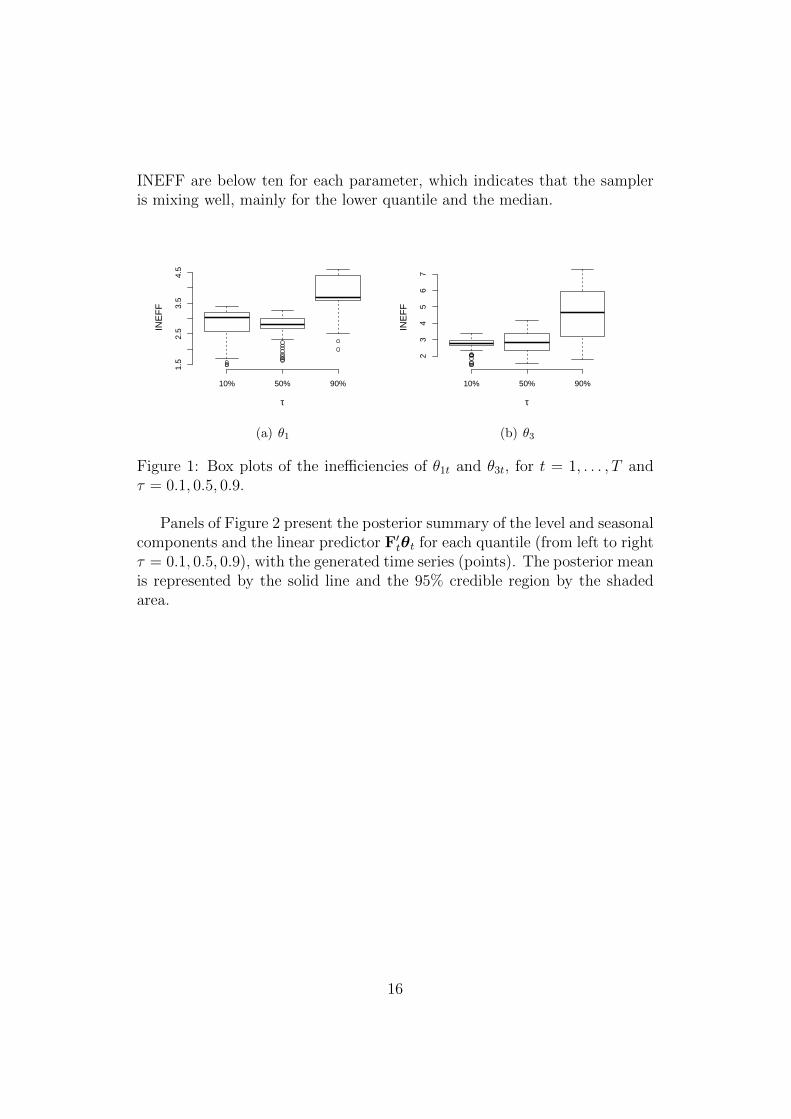
INEFF are below ten for each parameter, which indicates that the sampleris mixing well, mainly for the lower quantile and the median.

τ

INE

FF

10% 50% 90%

1.5

2.5

3.5

4.5

(a) θ1

τIN

EF

F

10% 50% 90%

23

45

67

(b) θ3

Figure 1: Box plots of the inefficiencies of θ1t and θ3t, for t = 1, . . . , T andτ = 0.1, 0.5, 0.9.

Panels of Figure 2 present the posterior summary of the level and seasonalcomponents and the linear predictor F′tθt for each quantile (from left to rightτ = 0.1, 0.5, 0.9), with the generated time series (points). The posterior meanis represented by the solid line and the 95% credible region by the shadedarea.

16

0 20 40 60 80 100

040

80

Time

Leve

l

0 20 40 60 80 100

−5

05

Time

Sea

son

0 20 40 60 80 100

040

80

Time

Qua

ntile

0 20 40 60 80 100

040

80

Time

Leve

l

0 20 40 60 80 100

−15

010

20

Time

Sea

son

0 20 40 60 80 100

040

80

Time

Qua

ntile

0 20 40 60 80 100

040

80

Time

Leve

l

0 20 40 60 80 100

−10

05

10

Time

Sea

son

0 20 40 60 80 100

040

80Time

Qua

ntile

(a) MCMC

0 20 40 60 80 100

040

80

Time

Leve

l

0 20 40 60 80 100

−5

05

Time

Sea

son

0 20 40 60 80 100

040

80

Time

Qua

ntile

0 20 40 60 80 100

040

80

Time

Leve

l

0 20 40 60 80 100

−15

010

20

Time

Sea

son

0 20 40 60 80 100

040

80

Time

Qua

ntile

0 20 40 60 80 100

040

80

Time

Leve

l

0 20 40 60 80 100

−10

05

10

Time

Sea

son

0 20 40 60 80 100

040

80

Time

Qua

ntile

(b) Approximated method

Figure 2: Smoothed posterior mean (solid line), 95% credible region (shadedarea) of the level and seasonal components for each quantile, based on theMCMC output (a) and in the approximated method (b). From left to rightτ = 0.1, 0.5, 0.9.

17

Figure 3 presents the plot of the estimated values of the linear predictorfor each quantile under MCMC approach versus the proposed approximatedalgorithm. The lengths of the segments represent the 95% credibility intervalobtained by MCMC approach. We conclude that both methods producesimilar results, but while MCMC takes about 5 minutes for 5,000 sweeps fora specific quantile, the approximated method takes seconds. Both algorithmswere implemented in the R programming language, version 3.4.1 (R CoreTeam 2017), in a computer with an Intel(R) Core(TM) i7-7700 processor3.60 GHz. This is first evidence of the relevance of the approximated DQLMto deal with a scalable dataset.

0 20 40 60

020

4060

Approximated

MC

MC

(a) 10%

0 20 40 60

020

4060

Approximated

MC

MC

(b) 50%

20 40 60 80 100

2060

100

Approximated

MC

MC

(c) 90%

Figure 3: Plot of the estimated values (posterior mean) of the linear predictorunder the MCMC inference approach versus the approximated method.

3.1.2 Non-Gaussian artificial dataset

To illustrate how the method works with a non-Gaussian dataset, wegenerated an artificial dataset from a first order dynamic gamma regressionwith mean µt, scale parameter φ and a canonical link function ηt = log(µt) =F′tθt. In particular, we generated T = 100 observations assuming Ft =(1, xt), where xt is an auxiliary variable at time t, Gt = I2×2, W = 0.01I2×2,for all t = 1, . . . , T and φ = 50. Each auxiliary variable xt was generatedindependently from a uniform distribution defined in the interval (2,4).

The model (4) was fitted to the original data and to the log transformeddata, for the quantiles 0.10, 0.50, and 0.90. We particularly choose hereto do the inference using only the MCMC algorithm. Although quantileregression is invariant to monotonic transformations, that is, the quantiles ofthe transformed variable are the transformed quantiles of the original variable(Koenker 2005, chapter 2, p. 34), the estimates of all the involved quantitieswere noticeably better when the data were transformed.

18

In order to validate the former result, some simulation studies weredeveloped. Several samples were generated from the gamma model. A simplestatic model is proposed in this exercise, with Ft = 1 and Wt = 0, for allt = 1, . . . , T . Fifty replications of samples of sizes T = 100 and T = 250 weregenerated using three different levels of skewness.

Figure 4 reports the empirical nominal coverage of the 95% credibilityintervals measured in percentages and the relative mean absolute error(RMAE) for the posterior mean of the quantiles for each case. The RMAEdecreases when we apply the AL to the logarithm of the sample observationsand also as the sample size increases or the distribution becomes moresymmetrically distributed. The desired nominal level of 95% is best achievedwhen the logarithm of the sample is considered, mainly as the level ofasymmetry decreases. The improvement in the results when using the logtransformation is more noticeable as the skeweness decreases.

Skewness = 0.47

τ

Cov

erag

e (%

)

2040

6080

10% 50% 90%

Skewness = 0.78

τ

10% 50% 90%

Skewness = 1.28

τ

10% 50% 90%

τ

RM

AE

0.00

0.04

0.08

0.12

10% 50% 90%

τ

10% 50% 90%

τ

10% 50% 90%

Figure 4: Empirical nominal coverage of the 95% credibility intervals (%) andthe MAE for the posterior mean of the quantiles for each case. The symbols• and N represent the results obtained when fitting the quantile regressionto the logarithm of the observations for T = 100 and T = 250, respectively.◦ and M represent the same results when the quantile regression is applied tothe observations on the original scale for T = 100 and T = 250, respectively.

19

Those results encourage us, as a future work, to explore in this contextthe idea of using the AL distribution for random effects in the link function,instead of applying it to the transformed response variable.

3.2 Real data example: Nile River flow

In this section we revisit a classic univariate time series previously analyzedin the literature. We apply the proposal to the annual flow of the Nile Riverat Aswan from 1871 to 1970 (Cobb 1978). This series shows level shifts, so weconsidered here a model which includes change points or structural breaks.The dataset is available in the R software (R Core Team 2017).

We also apply the proposal to a well-known toy example with the timeseries of quarterly gas consumption in the UK from 1960 to 1986, in whichthere is a possible change in the seasonal factor around the third quarter of1970 in Appendix 4.

The dataset in Figure 5 corresponds to the measurements of the annualflow of Nile River at Aswan (Egypt) from 1871 to 1970. The time series showslevel shifts. The construction of the first dam of Aswan started in 1898 andthe second big dam was completed in 1971, which caused enormous changeson the Nile flow and in the vast surrounding area. The application of aquantile model for this kind of dataset could be interesting to determine, forexample, the return period of a flood. The return period R(y) is defined to bethe mean value of a geometric distributed random variable with probabilityparameter P (y > y∗) = 1− τ . Then, R(y) = 1/(1− τ).

In order to capture these possible level changes we consider here a modelthat does not assume a regular pattern and stability of the underlying system,but can include change points or structural breaks.

Time

1871 1891 1911 1931 1951 1970

600

800

1200

Figure 5: Measurements of the annual flow of Nile River at Aswan from 1871to 1970.

20

A simple way to account for observations that are unusually far fromtheir one step-ahead predicted value is to describe the evolution error usinga heavy-tailed distribution. The Student-t distribution family is particularlyappealing in this respect for two reasons: (i) the Student-t distributionadmits a simple representation as a scale mixture of normal distributions,which allows one to treat a DLM with t-distributed observation errors asa Gaussian DLM, conditional on the scale parameters; and (ii) the FFBSalgorithm can still be used. Thus, we consider, the DQLM with evolutioncharacterized by the Student-t distribution, given by:

θt ∼ N(Gtθt−1, λ−1t W),

λt ∼ Ga(ν/2, ν/2), t = 1, . . . , T.(15)

The latent variable λ−1t can be informally interpreted as the degree of non-Gaussianity of wt. In fact, values of λ−1t lower than 1 make larger absolutevalues of wt more likely. Hence, the posterior distribution of λ−1t can beused to flag possible outliers. Through its degree-of-freedom parameter ν,which may also vary on time, different degrees of heaviness in the tails canbe attached. This class of models is discussed in Petris et al. (2009).

In this example, we fitted a first-order polynomial dynamic model, thuswe assumed Ft = Gt = 1 in model (4). We fitted the model (15) and the onewith normal evolution, for the 0.25, 0.5, and 0.75-quantiles.

In both cases, for the variance of the states W , we considered a half-Cauchy prior distribution, discussed by Gelman (2006), with scale 25, set asa weakly informative prior distribution. Although we could even assume aprior distribution for this, as described in Petris et al. (2009), we assumed νknown a priori and fixed at 2.5.

Figure 6 shows the linear predictor for each quantile, with its 95%credibility interval represented by the shaded area, obtained from the normal(first column) and Student-t fits (second column). Model (15) results insmoother linear predictors with more accurate credibility intervals.

21

25 %

Time

1880 1900 1920 1940 1960

600

800

1000

1200

1400

25 %

Time

1880 1900 1920 1940 1960

600

800

1000

1200

1400

50 %

Time

1880 1900 1920 1940 1960

600

800

1000

1200

1400

50 %

Time

1880 1900 1920 1940 1960

600

800

1000

1200

1400

75 %

Time

1880 1900 1920 1940 1960

600

800

1000

1200

1400

(a) Normal

75 %

Time

1880 1900 1920 1940 1960

600

800

1000

1200

1400

(b) Student-T

Figure 6: Posterior mean of the linear predictor (represented by the solidline) and the 95% credible region (represented by the shaded area) for eachquantile, under normal and student-t evolution.

22

Table 1 presents the posterior mean of the linear predictor for the 0.25,0.5, and 0.75-quantiles for the model with normal and Student-t evolutionaround the year 1899. The abrupt regime change is better captured in theStudent-t than in the normal model for all quantiles.

Table 1: Posterior mean of the linear predictor for the 0.25, 0.5, and 0.75-quantiles of the model with normal and Student-t evolution.

Student-t NormalYear 25% 50% 75% 25% 50% 75%1896 1064.01 1134.51 1219.03 1046.11 1124.00 1216.961897 1004.97 1083.83 1147.69 984.23 1064.32 1137.241898 959.51 1047.47 1117.77 922.98 1016.65 1093.481899 792.07 890.29 972.25 836.57 943.65 999.191900 784.17 871.67 938.27 814.69 903.88 949.231901 771.33 863.93 926.85 794.25 882.78 930.59

Figure 7 shows the boxplots of the posterior distribution of λ−1t inlogarithmic scale from 1871 to 1970 for each quantile. Values of log λ−1tgreater than 0 indicate an abrupt regime change. Boxplots in gray do notinclude the value 0. Thus, it is possible to observe that the model in factaccommodates the outliers. The regime change in 1899 is detected for allthe quantile regression models fitted. However, for the 0.75-quantile otheroutliers were detected.

23

1871 1880 1889 1898 1907 1916 1925 1934 1943 1952 1961 1970

01

23

4

25 %

Time

log

λ t−1

1871 1880 1889 1898 1907 1916 1925 1934 1943 1952 1961 1970

01

23

4

50 %

Time

log

λ t−1

1871 1880 1889 1898 1907 1916 1925 1934 1943 1952 1961 1970

−0.

51.

02.

5

75 %

Time

log

λ t−1

Figure 7: Boxplots of the posterior samples of λ−1t in log scale for the 0.25,0.5, and 0.75 quantiles over the years.

3.3 Tuberculosis cases in Rio de Janeiro

According to the World Health Organization (WHO), tuberculosis (TB) isone of the top 10 causes of death worldwide. Brazil is one of the countrieswith the highest number of cases in the world and since 2003 the disease hasbeen considered a priority by the Brazilian Ministry of Health. As part ofthe overall effort to reduce the incidence and mortality rate, the Ministry ofHealth, through the General Office to coordinate the National TuberculosisControl Program (CGPNCT), prepared a national plan to end tuberculosisas a public health problem in Brazil, reaching at target of less than 10 casesper 100,000 inhabitants by 2035. The plan to end the TB epidemic is a targetunder the Sustainable Development Goals that requires implementing a mixof biomedical, public health and socioeconomic interventions along with

24

research and innovation. The World Health Assembly passed a resolutionapproving with full support the new post-2015 End TB Strategy with itsambitious targets (WHO 2014).

The state of Rio de Janeiro is located in southeastern Brazil, with over16 million residents in 2017. The Rio de Janeiro state has one of the highestTB rates in the country. In 2015, there were 13,094 new notified cases,representing 15% of new cases for the whole country. We fit the proposedDQLM with a trend component for monthly incidence in Rio de Janeiro fromJanuary 2001 to December 2015. Figure 8 (a) presents the posterior mean(dashed line) and the 95% credibility interval (region in gray) for the linearpredictor for the 0.1, 0.5, and 0.9-quantiles, under the MCMC procedure.Figure 8 (b) presents the posterior summary of the interquantile range (IQR)between 10% and 90%. It is possible to observe a decreasing pattern for theIQR, mainly after 2008.

Time

Inci

denc

e/ 1

00 th

ousa

nd in

hab

2001 2006 2011 2016

67

89

10

(a)

Time

IQR

/ 100

thou

sand

inha

b

2001 2005 2008 2012 2016

0.5

1.0

1.5

2.0

2.5

(b)

Figure 8: Monthly incidence of TB in Rio de Janeiro state: (a) Posteriormean (dashed line) of the linear predictor for the 0.1, 0.5, and 0.9-quantiles,and their 95% credibility intervals for the 0.1 and 0.9-quantiles; (b) Posteriorsummary for the interquantile range between the 0.1 and 0.9 quantiles.

One of the targets of the post-2015 global tuberculosis strategy is a20% reduction in tuberculosis incidence by 2020, compared with 2015, a50% reduction by 2025, an 80% reduction by 2030 and a 90% reductionin tuberculosis incidence by 2035, compared with 2015. In particular, theinterest here is to predict the incidence from January 2016 to December2020, in order to detect in terms of the median, if the target can be achieved.

In MCMC inference procedure, samples from θT+k, k a non-negativeinteger, are obtained by propagating the samples from the posterior

25

distribution through the evolution equation (4). In the approximatedmethod, this is done after estimating φ through maximum posteriorestimation. Hence, we get that:

θ∗T+k | DT ∼ [a∗T+k, φ−1R∗T+k], (16)

where a∗T+k = GT+ka∗T+k−1 and C∗T+k = GT+kR

∗T+k−1G

′T+k can be

recursively calculated.In order to capture the steep decline of new cases that represents the

government target, we considered beside a linear forecast function in theoriginal scale, a linear forecast for the log-transformation to the dataset andtwo higher-order models. First, we considered a quadratic growth DLM(West and Harrison 1997, chapter 7, p. 223), which is obtained specifying in

equation (2) Ft = (1, 0, 0)′, Gt =

1 1 10 1 10 0 1

and Wt a diagonal matrix.

Then, we considered a locally approximation by a second-order Taylorexpansion to the non-linear Gompertz-type forecast functions (Harrison et al.1977). The Gompertz function evolves three parameters and is defined by:

g(t) = At +Bt exp(Ctt). (17)

To deal with the non-linear form, the quadratic polynomial DLM,previously described, was used for updating the corresponding threeparameters, then, the form in (17) was converted back and the full non-linearform used for the forecast function.

Figure 9 presents the forecast from 2016 to 2020 of the median of themonth incidence of TB per 100 thousand inhabitants for both alternativespreviously described, under the MCMC approach, for the four modelspreviously described. The dashed line represents the posterior mean, theregion in gray the 95% credibility interval and the red line indicates theTB reduction targets calculated for Rio de Janeiro state using 2015 as thebaseline.

According to all four models, the WHO’s 2020 target, estimated by 5.28cases per month per 100 thousand inhabitants, can be achieved in Rio deJaneiro. The Gompertz model captures the steep decline and it estimatesfor January 2020 a TB incidence of 5.19 (95%CI = (3.15, 8.29)) TB cases per100 thousand inhabitants. As in the Gompertz model fitting, we estimateBT < 0 (mean = - 0.99, 95%CI =(-1.12, -0.96)) and CT > 0 (mean =0.04, 95%CI =(-0.11, 0.18)), g(t) defined in (17) is a non-increasing modelconverging to At as t → ∞. Thus, considering a typical stagnation of thedisease incidence, the Gompertz model seems to be the more appropriate tocapture such long-term forecasts.

26

2001 2006 2011 2016 2020

35

79

11

Time

Inci

denc

e/ 1

00 th

ousa

nd in

hab

(a) Linear growth DLM

2001 2006 2011 2016 2020

35

79

11

Time

Inci

denc

e/ 1

00 th

ousa

nd in

hab

(b) Quadratic growth DLM

2001 2006 2011 2016 2020

35

79

11

Time

Inci

denc

e/ 1

00 th

ousa

nd in

hab

(c) Gompertz model

2001 2006 2011 2016 2020

35

79

11

Time

Inci

denc

e/ 1

00 th

ousa

nd in

hab

(d) Linear growth DLM - log data

Figure 9: Temporal predictions of monthly incidence of TB in Rio deJaneiro state from January 2016 to December 2020. The line represents theobserved time series and the dashed line represents the mean of the predictivedistribution for the median (0.5-quantile), the region in gray represents the95% credibility interval and the red line the WHO’s reduction target, undereach model considered.

4 Conclusions

In this article we propose a new class of models, named dynamic quantilelinear models. For the inference procedure, we develop two approaches: (i)a MCMC algorithm based on Gibbs sampling and FFBS for the modelof the location-scale mixture representation of the asymmetric Laplacedistribution; and (ii) a faster sequential method, based on approximationsusing Kullback-Leibler divergence and Bayes linear method. The secondinference approach has the advantage of being computationally cheaper. Asuggested alternative approach is the use of SMC methods for online state

27

and parameter estimation in the state-space model proposed. In particular,the approach presented in Yang et al. (2018) could be applied to the DQLMin (2) and (4). The approach considers filtering and smoothing methodsvia SMC for general state space models in the context of state and fixedparameters, providing a correction to the smoothing methods proposed byCarvalho et al. (2010). However, as illustrated by Yang et al. (2018) thefiltering and smoothing methods with SMC could have almost the samecomputational time of a MCMC.

We evaluated the DQLM in artificial and real datasets. In the simulationstudy, we applied our model in a Gaussian example with trend and seasonalcomponents where the DQLM performed well, and the approximate DQLMwas a computationally efficient alternative to MCMC. We also applied ourmodel in a non-Gaussian example generated by a gamma model encouragingthe investigation of introducing the AL model in the link function, or in theresponse variable. In the classic real Nile River data example, we illustratedby fitting a model for outliers and structural breaks that the detection ofoccasional abrupt changes differs depending on the quantile of interest.

The application to the tuberculosis data in Rio de Janeiro, Brazil,illustrates the practical importance of evaluating quantiles instead of themean in the context of forecasting. It also encourages us to extendthe proposal to joint modeling for the quantiles and a dynamic quantilehierarchical model. In particular, our method can be applied to any infectiousdisease, once it is important to assess whether public health policies areeffective, not only in reducing the trend in the number of cases, but also thevariability of number of total cases. Moreover, the upper quantiles can beuseful for early detection of an outbreak (epidemic). If the distribution of thenumber of cases (represented by the quantiles) is much higher than usual, itis a strong indication that attention is required.

References

R. Alhamzawi, K. Yu, and J. Pan. Prior elicitation in Bayesian quantileregression for longitudinal data. Journal of Biometrics & Biostatistics, 2(3):1–7, 2011. doi: 10.4172/2155-6180.1000115.

G. W. Bassett Jr and H.-L. Chen. Portfolio style: Return-basedattribution using quantile regression. In Economic Applications of QuantileRegression, pages 293–305. Springer, 2002.

L. S. Bastos and D. Gamerman. Dynamic survival models with spatial frailty.Lifetime Data Analysis, 12(4):441–460, 2006.

28

J. M.-M. B. Bernardo. Bioestadıstica: una perspectiva bayesiana. Number61: 311. Vicens-vives, 1981.

Z. Cai. Regression quantiles for time series. Econometric Theory, 18(01):169–192, 2002.

C. K. Carter and R. Kohn. On gibbs sampling for state space models.Biometrika, 81(3):541–553, 1994.

C. M. Carvalho, M. S. Johannes, H. F. Lopes, N. G. Polson, et al. Particlelearning and smoothing. Statistical Science, 25(1):88–106, 2010.

G. W. Cobb. The problem of the nile: conditional solution to a changepointproblem. Biometrika, 65(2):243–251, 1978.

C. Da-Silva, H. S. Migon, and L. Correia. Dynamic bayesian beta models.Computational Statistics & Data Analysis, 55(6):2074–2089, 2011.

A. Doucet, N. De Freitas, and N. Gordon. An introduction to sequentialmonte carlo methods. In Sequential Monte Carlo methods in practice,pages 3–14. Springer, 2001.

J. Durbin and S. J. Koopman. A simple and efficient simulation smootherfor state space time series analysis. Biometrika, 89(3):603–616, 2002.

M. V. Fernandes, A. M. Schmidt, and H. S. Migon. Modelling zero-inflatedspatio-temporal processes. Statistical Modelling, 9(1):3–25, 2009.

M. A. Ferreira, S. H. Holan, and A. I. Bertolde. Dynamic multiscalespatiotemporal models for gaussian areal data. Journal of the RoyalStatistical Society: Series B (Statistical Methodology), 73(5):663–688, 2011.

T. C. O. Fonseca and M. A. R. Ferreira. Dynamic multiscale spatiotemporalmodels for poisson data. Journal of the American Statistical Association,112(517):215–234, 2017. doi: 10.1080/01621459.2015.1129968.

S. Fruhwirth-Schnatter. Data augmentation and dynamic linear models.Journal of Time Series Analysis, 15(2):183–202, 1994.

D. Gamerman and H. F. Lopes. Markov chain Monte Carlo: stochasticsimulation for Bayesian inference. Chapman and Hall/CRC, 2006.

D. Gamerman, A. R. Moreira, and H. Rue. Space-varying regression models:specifications and simulation. Computational Statistics & Data Analysis,42(3):513–533, 2003.

29

A. Gelman. Prior distributions for variance parameters in hierarchical models(comment on article by Browne and Draper). Bayesian Analysis, 1(3):515–534, 2006.

P. J. Harrison and C. F. Stevens. Bayesian forecasting. Journal of the RoyalStatistical Society. Series B (Methodological), 38(3):205–247, 1976.

P. J. Harrison, T. Leonard, and T. N. Gazard. An application of multivariatehierarchical forecasting. Technical Report 15, Department of Statistics,University of Warwick., 1977.

B. Jorgensen. Statistical properties of the generalized inverse Gaussiandistribution, volume 9. Springer Science & Business Media, 2012.

R. Koenker. Quantile regression. Number 38. Cambridge university press,2005.

R. Koenker and G. Bassett. Regression quantiles. Econometrica, 46(1):33–50,January 1978.

R. Koenker and Z. Xiao. Quantile autoregression. Journal of the AmericanStatistical Association, 101(475):980–990, 2006.

S. Kotz, T. Kozubowski, and K. Podgorski. The Laplace distribution andgeneralizations: a revisit with applications to communications, economics,engineering, and finance. Springer Science & Business Media, 2001.

H. Kozumi and G. Kobayashi. Gibbs sampling methods for Bayesian quantileregression. Journal of Statistical Computation and Simulation, 81(11):1565–1578, 2011.

A. A. Kudryavtsev. Using quantile regression for rate-making. Insurance:Mathematics and Economics, 45(2):296–304, 2009.

D. Kuonen. Numerical integration in S-PLUS or R: A survey. Journal ofStatistical Software, 8(13):1–14, 2003.

R. Li, X. Huang, and J. Cortes. Quantile residual life regression withlongitudinal biomarker measurements for dynamic prediction. Journal ofthe Royal Statistical Society: Series C (Applied Statistics), 65(5):755–773,2016.

H. F. Lopes, E. Salazar, D. Gamerman, et al. Spatial dynamic factor analysis.Bayesian Analysis, 3(4):759–792, 2008.

30

Y. Luo, H. Lian, and M. Tian. Bayesian quantile regression for longitudinaldata models. Journal of Statistical Computation and Simulation, 82(11):1635–1649, 2012.

H. S. Migon and L. C. Alves. Multivariate dynamic regression: modelingand forecasting for intraday electricity load. Applied Stochastic Models inBusiness and Industry, 29(6):579–598, 2013.

H. S. Migon, D. Gamerman, H. F. Lopes, and M. A. Ferreira. Handbookof statistics. Bayesian statistics: modeling and computation, volume 25,chapter Bayesian dynamic models, pages 553–588. Elsevier, 2005.

B. Neelon, F. Li, L. F. Burgette, and S. E. Benjamin Neelon. Aspatiotemporal quantile regression model for emergency departmentexpenditures. Statistics in Medicine, 34(17):2559–2575, 2015.

L. Peng, J. Xu, and N. Kutner. Shrinkage estimation of varying covariateeffects based on quantile regression. Statistics and Computing, 24(5):853–869, 2014.

G. Petris, S. Petrone, and P. Campagnoli. Dynamic Linear Models with R.Springer-Verlag, 2009.

R. Prado and M. West. Time series: modeling, computation, and inference.CRC Press, 2010.

R Core Team. R: A Language and Environment for Statistical Computing.R Foundation for Statistical Computing, Vienna, Austria, 2017. URLhttp://www.R-project.org/.

M. A. Rahman. Bayesian quantile regression for ordinal models. BayesianAnalysis, 11(1):1–24, 2016.

R. R. Ravines, A. M. Schmidt, H. S. Migon, and C. D. Renno. A joint modelfor rainfall–runoff: the case of rio grande basin. Journal of Hydrology, 353(1-2):189–200, 2008.

W. J. Reed. The normal-Laplace distribution and its relatives. In Advancesin Distribution Theory, Order Statistics, and Inference, pages 61–74.Springer, 2006.

B. J. Reich. Spatiotemporal quantile regression for detecting distributionalchanges in environmental processes. Journal of the Royal StatisticalSociety: Series C (Applied Statistics), 61(4):535–553, 2012.

31

B. J. Reich and L. B. Smith. Bayesian quantile regression for censored data.Biometrics, 69(3):651–660, 2013.

B. J. Reich, M. Fuentes, and D. B. Dunson. Bayesian spatial quantileregression. Journal of the American Statistical Association, 106(493):6–20, 2011.

N. Shephard. Partial non-Gaussian state space. Biometrika, 81(1):115–131,1994.

M. A. O. Souza, H. S. Migon, and J. B. M. Pereira. Extendeddynamic generalized linear models: the two-parameter exponential family.Computational Statistics & Data Analysis, 121(5):164–179, 2018.

K. Sriram, P. Shi, and P. Ghosh. A Bayesian quantile regression model forinsurance company costs data. Journal of the Royal Statistical Society:Series A (Statistics in Society), 179(1):177–202, 2016.

J. W. Taylor. A quantile regression approach to estimating the distributionof multiperiod returns. The Journal of Derivatives, 7(1):64–78, 1999.

M. West. Robust sequential approximate bayesian estimation. Journal ofthe Royal Statistical Society (Ser. B), 43:157–166, 1981.

M. West and J. Harrison. Bayesian Forecasting and Dynamic Models.Springer, 1997.

M. West, P. J. Harrison, and H. S. Migon. Dynamic generalized linear modelsand bayesian forecasting. Journal of the American Statistical Association,80(389):73–83, 1985.

WHO. Draft global strategy and targets for tuberculosis prevention, care andcontrol after 2015. Documentation for World Health Assembly 67 A67/11,World Health Organization, 2014.

B. Yang, J. R. Stroud, and G. Huerta. Sequential monte carlo smoothingwith parameter estimation. Bayesian Analysis, 2018.

Y. Yang, H. J. Wang, and X. He. Posterior inference in Bayesian quantileregression with asymmetric Laplace likelihood. International StatisticalReview, 84(3):327–344, 2016.

K. Yu and R. A. Moyeed. Bayesian quantile regression. Statistics &Probability Letters, 54(4):437–447, 2001.

32

Y. Yu. Bayesian quantile regression for hierarchical linear models. Journalof Statistical Computation and Simulation, 85(17):3451–3467, 2015.

Y. R. Yue and H. Rue. Bayesian inference for additive mixed quantileregression models. Computational Statistics & Data Analysis, 55(1):84–96, 2011.

Z. Y. Zhao, M. Xie, and M. West. Dynamic dependence networks: Financialtime series forecasting and portfolio decisions. Applied Stochastic Modelsin Business and Industry, 32(3):311–332, 2016.

33

Appendix 1: Proof of Lemma 2.2

Lemma 2.2

(i) Let us find a tractable monotone transformation ζ = ζ(θ) to inducenormality in the sense of minimizing the divergence measure between p(ζ)and its normal approximation. In particular we have θ ∼ Ga(a, b). This isequivalent to finding ζ that minimizes the expected value

k[p(ζ), q(ζ)] =

∫p(ζ) log

p(ζ)

q(ζ)dζ,

where q(ζ) is the density function of the N [E(ζ), V (ζ)] distribution andp(ζ) = p(θ)/|dζ/dθ|.

Thus, we want a function ζ which minimizes

k[p(ζ), q(ζ)] =

∫p(ζ) log p(ζ)dζ −

∫p(ζ) log q(ζ)dζ

=

∫p(ζ) log p(ζ)dζ +

1

2log(2πV (ζ))

∫p(ζ)dζ +

∫p(ζ)

[(ζ − E(ζ))2

2V (ζ)

]dζ

=

∫p(ζ) log p(ζ)dζ +

1

2log(2πV (ζ)).

We consider the class of transformations ζ = ζ(θ), such that dζ/dθ = θ−α,0 ≤ α ≤ 1, which contains as particular cases the standard transformations:

ζ(θ) =

θ, for α = 0,log θ, for α = 1,(1− α)θ1−α, for α < 1.

We have∫p(ζ) log p(ζ)dζ =

∫p(θ) log p(θ)dθ −

∫log ζ ′(θ)p(θ)dθ

= C1 + α

∫log θp(θ)dθ = C1 + αE(log θ) ≈ C + α

(log

a

b− 1

2a

).

Moreover, using that V (ζ) ≈ [ζ ′(E(θ))]2 V (θ), we get log(2πV (ζ)) =2α log (b/a) + C2. Then,

k[p, q] = α

(log

b

a− 1

2a

)+ C,

34

which is a decreasing function in α for the particular values that a and bcan assume in the method. It follows that progressively better normalizingtransformations are obtained for larger values of α. Thus, in this class oftransformations, ζ(θ) = log θ is the one which minimizes the divergencemeasure between p(ζ) and its normal approximation.

(ii) If we have ζ ∼ N [µ, σ2], such that µ = E(ζ) and σ2 = V (ζ), thenθ = exp(ζ) has distribution LN [µ, σ2] and we desire the better Ga(a, b)to approximate this lognormal distribution in the sense of Kullback-Leiblerdivergence. That is, we want a and b which minimize

k[p(θ), q(θ)] =

∫p(θ) log p(θ)dθ −

∫p(θ) log q(θ)dθ,

or maximizes

f(a, b) =

∫p(θ) log q(θ)dθ,

where q(θ) and p(θ) are the density functions of the Ga(a, b) and LN(µ, σ2)distribution, respectively.

Thus,

f(a, b) =

∫p(θ) log q(θ)dθ =

∫(a log b− log(Γ(a)) + (a− 1) log(θ)− bθ) p(θ)dθ

= a log b− log(Γ(a)) + (a− 1)ELN(log(θ))− bELN(θ)

= a log b− log(Γ(a)) + (a− 1)µ− b exp(µ+ σ2/2

).

Deriving it with respect to a and b and setting equal to zero, we get thatthe maximum of f(a, b) is achieve when:

a = σ−2 and b = σ−2 exp

[−(µ+

σ2

2

)],

for σ2 < 1, in order to guarantee the existence of the mode of the gammadistribution.

Appendix 2: NGAL distribution

This distribution was first presented in Reed (2006), who described someof its properties. A random variable Y has a NGAL distribution if itscharacteristic function is equal to

ϕy(s) =

(αβ exp(iδs− γs2/2)

(α− is)(β − is)

)ρ, (18)

35

where α, β, ρ and γ are positive parameters and δ is real. We write Y ∼NGAL(δ, γ, α, β, ρ) to indicate that Y follows such a distribution. Using thecumulants of the distribution it is possible to obtain:

E(Y ) = ρ

(δ +

1

α− 1

β

)and V ar(Y ) = ρ

(γ +

1

α2+

1

β2

).

Also, the coefficients of kurtosis and skewness are, respectively, given by:

k4k22

=6(α4 + β4)

ρ(γα2β2 + α2 + β2)2and

k3

k3/22

=2(β3 − α3)

ρ1/2(γα2β2 + α2 + β2)2.

Figure 10 compares the density curves of NGAL for some values of theparameters. It is possible to observe that as σ2 increases, the density becomesboth wider and flatter. The parameters α and β affect, respectively, theupper and lower tail behavior of the NGAL distribution: small values of αand β correspond, respectively, to a fat upper and lower tails, while as theyincrease, the upper and lower tails of the distribution reduce to those of anormal distribution. Finally, as ρ increases both mean and variance increase.

−10 −5 0 5 10

0.00

0.10

0.20

0.30

Den

sity

µ = 0µ = − 3µ = 3

−10 −5 0 5 10

0.00

0.10

0.20

0.30

Den

sity

γ = 0γ = − 3γ = 3

−10 −5 0 5 10

0.00

0.10

0.20

0.30

Den

sity

c = 1c = 3c = 5

−10 −5 0 5 10

0.00

0.10

0.20

0.30

Den

sity

κ = 1κ = 4κ = 9

−10 −5 0 5 10

0.00

0.10

0.20

0.30

Den

sity

α = 0.5α = 2α = 5

−10 −5 0 5 10

0.0

0.1

0.2

0.3

Den

sity

β = 2β = 0.5β = 0.1

Figure 10: Density function of the NGAL distribution with some differentvalues of the parameters.

Finally, we need to prove that the distribution described in Theorem 2.3is a NGAL distribution. In order to facilitate the notation, let us omit the

36

index t and call: θ = F′tat, µ = aτφ−1/2β−1t , σ2 = φ−1bτβ

−1t , c = φ−1F′tRtFt,

ρ = αt and w = Ut. Thus, we have:

y | w ∼ N(θ + µw, c+ σ2w

),

w ∼ Ga(ρ, 1).

Conditional on w, we obtain the ch.f of y as:

ϕy(s) = E[E(eisy | w

)]= eisθ

∫ ∞0

eisµwE(eis(c+σ

2w)1/2z)g(w)dw

= eisθ1

Γ(α)

∫ ∞0

eisµwe−12s2(c+σ2w)wα−1e−wdw

= eisθ−12s2c 1

Γ(α)

∫ ∞0

wα−1e−w(1+ 12σ2s2−iµs)dw

= eisθ−12s2c

(1

1 + 12σ2s2 − iµs

)ρ. (19)

Thus, ϕY (s) = ϕε(s).ϕζ(s), where ϕε(s) is the N(0, c) ch.f and ϕζ(s) is theGAL(θ, µ, σ, ρ) ch.f. Thus, it follows that the NGAL distribution is that ofthe convolution of the normal N(0, c) and GAL(θ, µ, σ, ρ) distributions, thatis Y = ζ + ε, for independent ζ and ε.

Moreover, the ch.f in (19) can be expressed as stated in (18), for α = 2κ√2σ

,

β = 2√2σκ

, δ = θ/ρ, γ = c/ρ and the additional parameter κ > 0 is related toµ and σ as follows:

κ =

√2σ2 + µ2 − µ√

2σ, while µ =

σ√2

(1

κ− κ),

showing that it is NGAL distributed.

Appendix 3: Assessment by MCMC

Figure 11 shows the trace plot with the posterior distribution of parametersθt’s for some times for each quantile regression fitted. The chains in blackare obtained for quantile 0.10, in dark gray for quantile 0.50 and in light grayfor 0.90. The line represents the true value of each component of θt used inthe data generating process.

Figure 12 presents histograms of the posterior densities of some elementsof the covariance matrix W for the median, where the true value usedin the data generation process is given by the vertical dashed line. Thehyperparameters appear to be well estimated.

37

Iterations

θ 1

0 4000 8000

−10

05

15

0 4000 8000

−10

05

15

Iterations

θ 3

0 4000 8000

−5

05

10

0 4000 8000

−5

05

10

(a) t = 1

Iterations

θ 1

0 4000 8000

010

2030

0 4000 8000

010

2030

Iterations

θ 3

0 4000 8000

−5

05

0 4000 8000

−5

05

(b) t = 10

Iterations

θ 1

0 4000 8000

2535

4555

0 4000 8000

2535

4555

Iterations

θ 3

0 4000 8000

−5

05

0 4000 8000

−5

05

(c) t = 40

Iterations

θ 1

0 4000 8000

5060

7080

0 4000 8000

5060

7080

Iterations

θ 3

0 4000 8000

−10

−5

05

0 4000 8000

−10

−5

05

(d) t = 80

Figure 11: Trace plot with the posterior densities of θt’s for some times andσ for each quantile regression fitted.

38

W11D

ensi

ty

0.00 0.04

020

4060

W22

Den

sity

0.00 0.06

020

4060

80

W33

Den

sity

0.00 0.20

010

2030

40

W44

Den

sity

0.00 0.05

020

4060

W12

Den

sity

−0.02 0.02

020

4060

80

W13

Den

sity

−0.04 0.02

020

4060

Figure 12: Histograms with the posterior densities of the hyperparametersin the diagonal of the covariance matrix W for the median.

Appendix 4: A toy example: UK gas

consumption

The following dataset consists of quarterly UK gas consumption from 1960to 1986 (see Figure 13). The plot of the data suggests a possible change inthe seasonal factor around the third quarter of 1970.

Time

UK

gas

1960 1965 1970 1975 1980 1985

200

600

1000

Figure 13: Quarterly UK gas consumption from 1960 to 1986, in millions oftherms.

39

We employ a model built on a local linear trend plus a quarterly seasonalcomponent DLM to analyze the data, that is, we consider Ft = (1, 0, 1, 0, 0)′

and Gt =

1 1 0 0 00 1 0 0 00 0 −1 −1 −10 0 1 0 00 0 0 1 0

, for all t = 1, . . . , 108, in model (4).

We fit the DQLM for τ = 0.10, 0.50, 0.90 to the real dataset on the logscale. Figure 14 provides a plot of the posterior mean with the MCMCalgorithm (in black) and approximated method (in blue) of the trend andseasonal components, together with 95% credibility intervals using MCMC.It is possible to observe the change in the seasonal factor around the thirdquarter of 1970. Moreover, in terms of the posterior mean both methods arevery close to each other.

1960 1970 1980

34

56

7

Time

Leve

l

1960 1970 1980

−1.

50.

01.

02.

0

Time

Sea

son

1960 1970 1980

45

67

Time

Leve

l

1960 1970 1980

−1.

00.

01.

0

Time

Sea

son

1960 1970 1980

45

67

Time

Leve

l

1960 1970 1980

−1.

50.

01.

5

Time

Sea

son

Figure 14: Posterior mean (solid line), 95% credible region (shaded area) forthe level and seasonal components for each quantile.

40