dynamic reactive power control of isolated power … · 2017-04-28 · this dissertation presents...

DYNAMIC REACTIVE POWER CONTROL OF ISOLATED POWER SYSTEMS

A Dissertation

by

MILAD FALAHI

Submitted to the Office of Graduate Studies of Texas A&M University

in partial fulfillment of the requirements for the degree of

DOCTOR OF PHILOSOPHY

Approved by:

Co-Chairs of Committee, Mehrdad Ehsani Karen Butler-Purry Committee Members, Shankar Bhattacharyya John Hurtado Head of Department, Chanan Singh

December 2012

Major Subject: Electrical Engineering

Copyright 2012 Milad Falahi

ii

ABSTRACT

This dissertation presents dynamic reactive power control of isolated power

systems. Isolated systems include MicroGrids in islanded mode, shipboard power

systems operating offshore, or any other power system operating in islanded mode

intentionally or due to a fault. Isolated power systems experience fast transients due to

lack of an infinite bus capable of dictating the voltage and frequency reference. This

dissertation only focuses on reactive control of islanded MicroGrids and AC/DC

shipboard power systems. The problem is tackled using a Model Predictive Control

(MPC) method, which uses a simplified model of the system to predict the voltage

behavior of the system in future. The MPC method minimizes the voltage deviation of

the predicted bus voltage; therefore, it is inherently robust and stable. In other words,

this method can easily predict the behavior of the system and take necessary control

actions to avoid instability. Further, this method is capable of reaching a smooth voltage

profile and rejecting possible disturbances in the system. The studied MicroGrids in this

dissertation integrate intermittent distributed energy resources such as wind and solar

generators. These non-dispatchable sources add to the uncertainty of the system and

make voltage and reactive control more challenging. The model predictive controller

uses the capability of these sources and coordinates them dynamically to achieve the

voltage goals of the controller. The MPC controller is implemented online in a closed

control loop, which means it is self-correcting with the feedback it receives from the

system.

iii

DEDICATION

Dedicated to my parents who sparked my passion to learn, encouraged me to move

forward, and gave me the fear of being mediocre.

iv

ACKNOWLEDGEMENTS

I would like to thank my committee co-chairs for their patience and support. Special

thanks to Dr. Ehsani since I would not be able to finish this research without his help and

support. Thanks to Dr. Butler-Purry for her efforts to improve the quality of this

research, and for long pleasant discussions throughout my PhD at Texas A&M

University. I would also like to thank my committee members, Dr. Bhattacharyya, and

Dr. Hurtado, for their guidance and support throughout the course of this research.

Special thanks go to my friends and colleagues at Power System Automation Lab

(PSAL) and Sustainable Energy Vehicle Engineering and Power Electronics Lab for

their help and support during the long hard days that we spent together. I would also like

to thank the staff of Electrical Engineering Department for making my time at Texas

A&M University a great experience. Finally, thanks to my mother and father for their

encouragement and support throughout my studies at Texas A&M University.

Meanwhile, I hope this achievement is encouraging to my siblings that both selected to

do a PhD in Electrical Engineering at NC-State University and UCLA.

v

NOMENCLATURE

DER Distributed Energy Resource

DFIG Doubly Fed Induction Generator

DG Distributed Generator

MILP Mixed Integer Linear Programming

MIQP Mixed Integer Quadratic Programming

MLD Mixed Logical Dynamics

MPC Model Predictive Control

PWA Piecewise Affine System

SPS Shipboard Power System

STATCOM STAtic synchronous COMpensator

SVC Static Var Compensator

VVC Volt/Var Control

vi

TABLE OF CONTENTS

Page

ABSTRACT ................................................................................................................... .. ii

DEDICATION ............................................................................................................... . iii

ACKNOWLEDGEMENTS ........................................................................................... . iv

NOMENCLATURE ....................................................................................................... .. v

TABLE OF CONTENTS ............................................................................................... . vi

LIST OF FIGURES ........................................................................................................ viii

LIST OF TABLES ......................................................................................................... xiii

1. INTRODUCTION .................................................................................................... 1

1.1. Isolated Power Systems ............................................................................... 6

2. LITERATURE REVIEW OF REACTIVE POWER CONTROL METHODS OF DISTRIBUTION SYSTEMS .......................................................................... 18

2.1. Introduction ............................................................................................... 18 2.2. Network Model Based Techniques ........................................................... 19 2.3. Rule Base Techniques ............................................................................... 21 2.4. Intelligent Techniques ............................................................................... 22 2.5. Model Predictive Control (MPC) .............................................................. 22 2.6. Traditional Problem: Capacitor Placement and Sizing ............................. 23 2.7. Present Status of Reactive Power Control Methods of Isolated Power

Systems ................................................................................................... 29 2.8. Summary ................................................................................................... 40

3. DYNAMIC REACTIVE POWER CONTROL OF ISOLATED POWER SYSTEMS ............................................................................................................. 41

3.1. Introduction ............................................................................................... 41 3.2. Problem Formulation of Dynamic Reactive Power Control of Isolated

Power Systems .......................................................................................... 42 3.3. Model Predictive Control Based Reactive Power Control of Isolated

Power Systems ........................................................................................ 144 3.4. Performance Analysis of the MPC Controller ........................................ 155 3.5. Summary ................................................................................................. 160

vii

4. MODEL PREDICTIVE BASED REACTIVE POWER CONTROL OF SHIPBOARD POWER SYSTEMS .................................................................... 161

4.1. Introduction ............................................................................................. 161 4.2. Implementation and Simulation Results ................................................. 162 4.3. Local Control of DC Distribution Zones ................................................. 173 4.4. Summary ................................................................................................. 174

5. MODEL PREDICTIVE BASED REACTIVE POWER CONTROL OF MICROGRIDS .................................................................................................... 175

5.1. Introduction ............................................................................................. 175 5.2. Photovoltaic Source ................................................................................. 176 5.3. DFIG Wind Generator ............................................................................. 180 5.4. Connecting DERs to the Grid .................................................................. 182 5.5. Implementation and Simulation Results ................................................. 186 5.6. Summary ................................................................................................. 249

6. CONCLUSIONS AND FUTURE WORK .......................................................... 250

6.1. Conclusions ............................................................................................. 250 6.2. Future Research ....................................................................................... 251

REFERENCES ............................................................................................................. 253

APPENDIX A .............................................................................................................. 272

APPENDIX B .............................................................................................................. 274

viii

LIST OF FIGURES

Page

Figure 1-1 Magnitude-duration plot for classification of power quality events [2] ............................................................................................................... 5

Figure 1-2 A notional zonal AC/DC shipboard power system ...................................... 9

Figure 1-3 An example of possible hierarchical structure of MicroGrids ................... 14

Figure 1-4 An example of a zonal AC/DC MicroGrid [13] ........................................ 15

Figure 3-1 PWA model ................................................................................................ 51

Figure 3-2 Switched affine system .............................................................................. 53

Figure 3-3 Discrete hybrid automata [78] ................................................................... 55

Figure 3-4 Injection and withdrawal of reactive power from bus n ............................ 69

Figure 3-5 Converting the system to MLD form ......................................................... 70

Figure 3-6 Prediction of the voltage profile of buses in the system for MPC ............. 71

Figure 3-7 Sequence of control inputs ......................................................................... 72

Figure 3-8 General concept of model predictive control ............................................. 72

Figure 3-9 MLD constraints of the optimization problem at each step time ............... 73

Figure 3-10 Process of calculation of the objective function ........................................ 75

Figure 3-11 Actual synchronous generator voltage and estimated voltage using 1st and 2nd order models ......................................................................... 81

Figure 3-12 Schematic diagram of conventional control of DFIG wind generator ....... 81

Figure 3-13 Schematic diagram of conventional control of photovoltaic source .......... 85

Figure 3-14 Reactive response of a wind DG and the estimated reactive power .......... 86

Figure 3-15 Load current and voltage ........................................................................... 88

ix

Figure 3-16 Connection of synchronous generators and the rest of the network .......... 90

Figure 3-17 Bus angles for a MicroGrid for a case-study with changing loads ............ 92

Figure 3-18 A series feeder component ......................................................................... 95

Figure 3-19 Process of calculation of the objective function ........................................ 96

Figure 3-20 Transformer model .................................................................................... 99

Figure 3-21 Sample result of classification algorithm on 2 dimension data [112] ...... 104

Figure 3-22 Studies on a simple system ...................................................................... 107

Figure 3-23 Bus voltages of the simple 2 bus system ................................................. 111

Figure 3-24 Control inputs to the simple 2 bus system ............................................... 112

Figure 3-25 Control inputs to the simple 4 bus system ............................................... 113

Figure 3-26 Bus voltages of the system for 1 wind generator case ............................. 130

Figure 3-27 Control inputs to the system for 1 wind generator case ........................... 131











x

Figure 3-38 Flowchart of the MPC controller ............................................................. 146

Figure 3-39 The binary tree for a MIQP with 3 integer variables. Each node is marked with the corresponding vector [116] .................................... 148

Figure 3-40 Separation of the roots on the second variable [116] .............................. 149

Figure 3-41 Order of solving problems in the outside first strategy, assuming the “first free variable" branching rule [116] .............................................. 153

Figure 3-42 Block diagram of MPC for the MicroGrid .............................................. 155

Figure 4-1 Schematic diagram of a notional all electric shipboard power system ..................................................................................................... 163

Figure 4-2 High level schematic diagram of a notional all electric shipboard

power system .......................................................................................... 164 Figure 4-3 Control inputs to the SPS – Case study 1 ................................................ 169

Figure 4-4 Bus voltages of the SPS – Case study 1 ................................................... 169

Figure 4-5 Control inputs to the SPS – Case study 2 ................................................ 170



Figure 4-8 Control inputs to the SPS – Case study 3 ................................................ 173

Figure 4-9 Block diagram of local controller to control the voltage of DC zones .... 174

Figure 5-1 Control scheme of a DG unit [61] ........................................................... 178

Figure 5-2 Reactive power generation limits by the PV inverter [126] .................... 179

Figure 5-3 Schematic diagram of the studied MicroGrid .......................................... 187

Figure 5-4 RMS voltage of bus 5,6,7,8 – MPC (solid line), Local Control (dashed line) in case study 1 .................................................................. 193

Figure 5-5 Control inputs to the MicroGrid in case study 1 ...................................... 194

xi

Figure 5-6 Active and reactive response of wind generator 1 for case study 1 (solid line), control inputs (dotted line) .................................................. 195

Figure 5-7 Active and reactive response of the PV source for case study 1

(solid line) – control inputs (dotted line) ................................................ 195 Figure 5-8 Voltage of Bus 5,6,7,8 – MPC (solid line), Local Control (dashed

line) in case study 2 ................................................................................ 196 Figure 5-9 Control inputs to the MicroGrid in case study 2 ...................................... 197

Figure 5-10 RMS voltage of Bus 5,6,7,8 in case study 3 ............................................ 199


Figure 5-12 RMS voltage of Bus 5,6,7,8 in case study 4 ............................................ 201


Figure 5-14 MicroGrid based on the IEEE 34 node feeder ......................................... 203

Figure 5-15 Bus voltages with fixed capacitor – case study 1 .................................... 213

Figure 5-16 Bus voltages with fixed capacitor - case study 1 ..................................... 214

Figure 5-17 Bus voltages with MPC – case study 2 .................................................... 216


Figure 5-19 Control inputs to the MicroGrid generated by MPC – case study 2 ........ 218

Figure 5-20 Bus voltages of MicroGrid – case study 3 ............................................... 220

Figure 5-21 Bus voltages of the MicroGrid – case study 3 ......................................... 221


Figure 5-23 Active and reactive power generation of the wind generators – case study 3 .................................................................................................... 223



xii

Figure 5-26 Control inputs to the MicroGrid – case study 4 ....................................... 226










Figure 5-36 Wind profile ............................................................................................. 239







Figure 5-43 Bus voltages with MPC – case study 10 .................................................. 247

Figure 5-44 Bus voltages with MPC – case study 10 .................................................. 248

Figure 5-45 Control inputs to the MicroGrid generated by MPC – case study 10 ...... 249

xiii

LIST OF TABLES

Page Table 1 MicroGrid characteristics for different classes ............................................. 13

Table 2 Comparison of the available techniques for solving the VVC problem ....... 24

Table 3 MLD transform [78] ..................................................................................... 57

Table 4 Load and capacitor parameters of the 2 bus system ................................... 110

Table 5 Parameters of the 2 bus system ................................................................... 110

Table 6 Load parameters of the 4 bus system .......................................................... 122

Table 7 Classification of sub-problems according to guaranteed switches in the binary variables for nd = 3 [116] ......................................................... 152

Table 8 Generator parameters of the notional SPS .................................................. 167

Table 9 Load and line parameters of the notional SPS ............................................ 167

Table 10 AC line length of the notional SPS ............................................................. 168

Table 11 ANSI C84.1 voltage range for 120v [122] ................................................. 175

Table 12 Requested fault clearing time for isolated power systems .......................... 185

Table 13 Source parameters of the 11 bus MicroGrid ............................................... 187

Table 14 Sample of the MLD model for the studied MicroGrid ............................... 190

Table 15 Load and line parameters of the 11 bus MicroGrid .................................... 192

Table 16 Distributed loads of the IEEE 34 node system ........................................... 204

Table 17 Spot loads of the IEEE 34 node system ...................................................... 205

Table 18 Source parameters of the IEEE 34 node system ......................................... 205

Table 19 Power flow of the system when connected to the grid and the Diesel generator is off – Bus voltages ................................................................... 206

xiv

Table 20 Power flow of the system when connected to the grid and the Diesel

generator is off – Line currents ................................................................... 207 Table 21 Power flow of the system isolated from the grid – Bus voltages ............... 208

Table 22 Power flow of the system isolated from the grid – Line currents ............... 209

1

1 INTRODUCTION

An isolated power system is typically a small system that has no possibility of

support from an interconnected neighboring system due to a fault or intentional islanded

operation. Isolated systems commonly have limited generation capacity from local

distributed generators with small inertia. Due to minimal or non-existent transmission

system, isolated systems are more vulnerable to disturbances than stiff distribution

systems. These systems can easily move from one state to another due to load or

generation changes. Due to these distinguishing features, the power management

procedures of conventional terrestrial power systems cannot be effectively used for

isolated power systems. With these key traits in mind, it is desirable to develop a

dynamic power management scheme that accounts for the following criteria: economics,

reliability, security, and survivability. Dynamic is emphasized because system dynamics

or transients are very important when it comes to isolated power systems since load

demand is comparable to generation capacity.

The main objective of a dynamic power management scheme is to ensure continuous

power supply for electric loads with optimal utilization of power sources, thereby

enhancing system reliability and survivability. Dynamic power management strategy for

an isolated power system should include the following control modules that should work

together as needed to supply power to the loads: dynamic source management (economic

dispatch and unit commitment), dynamic phase/load balancing and grid management,

dynamic voltage and reactive power control, dynamic demand side management.

2

However, the proposed work in this dissertation only addresses dynamic reactive

control.

The objective of this dissertation is to develop a dynamic reactive power control

strategy for Volt/Var optimization of isolated systems. Volt/Var Optimization (VVO) or

generally Volt/Var Control (VVC) is concerned with coordinating the sources and sinks

of reactive power to achieve a smooth and stable voltage profile. Generally speaking,

bus voltage is coupled with reactive power in power systems. Therefore, coordinating

reactive power generation and consumption is helpful in keeping the bus voltages within

limits.

Load behavior as a response to voltage variation in a distribution system is very

important in volt/Var studies. Load studies show that typically about 50% of the loads in

a distribution system are motor loads. Motor loads in a conventional distribution system

are often a combination of industrial, residential and commercial motors [1]. The

remaining loads in the distribution system are typically constant power loads which can

be electronics, motor drives, etc. (about 20%), discharge lighting CFLs (about 10%) and

constant impedance loads which can be incandescent lighting, ranges, irons, etc. (about

20%). The behavior of each of these load types in response to voltage changes is

predictable. Discharge lighting usually turns off when voltage drops below 70 to 80%.

Adjustable speed drives temporarily shut down when the voltage level drops below 90%

and constant-impedance loads draw less active power from the network as the bus

voltage drops. Large industrial motors have contactors that turn the motor off when

voltage drops to about 75% and small motors such as those used in air-conditioning

3

which do not have electromagnetic contacts may stall, drawing large levels of current

from the power system when voltage sags to 70% or less.

In the stall condition, the motor continues to draw a large amount of current until it trips

the over current protection, which may take from 10 seconds up to a few minutes.

The amount of motor load has a significant impact on voltage stability of the isolated

distribution system. Small motors that do not disconnect are more problematic due to

stall at low voltage levels. Especially, low-inertia small motors that stall faster drag

down system voltage. Unfortunately, the new high-efficiency AC motors have

remarkably low inertia.

In the past, the induction motor’s speed slowed down slightly when its terminal

voltage dropped which resulted in a reduction in the total motor load. This reduction in

speed had a "healing" effect for the system when a voltage drop occurred in the system.

However, the new generation of adjustable speed drives, still supply the same voltage

and frequency to the motor even when the distribution bus voltage drops and thus

eliminate some of the inherent self-healing effect in the distribution system.

It is necessary to understand and classify the power quality problems in a power

system to be able to solve the problem [2]. There are different classifications for power

quality issues in distribution systems. Each of these classifications uses a specific

property to categorize the problem. Some standards classify the events as "steady-state"

or "non-steady-state" phenomena. Other standards such as ANSI C84.1 use the duration

of the event as the key factor for classification. Other guidelines such as IEEE-519 use

4

the wave shape of each event to classify power quality problems. Finally, standards such

as IEC use the frequency range of the event for the classification.

IEC presents the following list of phenomena causing electromagnetic disturbances:

Conducted low-frequency phenomena

1. Harmonics, interharmonics

2. Signaling voltage

3. Voltage imbalance

4. Power frequency variations

5. Induced low-frequency voltages

6. DC components in AC networks

7. Voltage fluctuations

8. Voltage dips

Radiated low-frequency phenomena

1. Electric fields

2. Magnetic fields

Conducted high-frequency phenomena

1. Unidirectional transients

2. Induced continuous wave (CW) voltages or currents

3. Oscillatory transients

Radiated high-frequency phenomena

1. Magnetic fields

2. Electric fields

5

3. Electromagnetic field

4. Steady-state waves

5. Transients

Electrostatic discharge phenomena (ESD)

Nuclear electromagnetic pulse (NEMP)

Although all the mentioned phenomena are considered as power quality issues, the

power system industry usually classifies power quality events according to their

magnitude and duration. A sample classification table of power quality issues based on

magnitude and duration of the event is shown in Figure 1-1.

Figure 1-1 Magnitude-duration plot for classification of power quality events [2]

There are nine different regions in the voltage-magnitude plot shown in Figure 1-1

and various standards give different names to events in each of these regions.

6

Classification based on the voltage magnitude divides power quality events into three

regions:

interruption: voltage magnitude is zero

Under-voltage: voltage magnitude is below its nominal value by a certain

percent

Over-voltage: voltage magnitude is above its nominal value by a certain

percent

Based on the duration of the event, these events are split into four regions, namely,

very short, short, long, and very long. The borders in this plot are somewhat arbitrary

and the user can set them according to the system requirements or the standard that is

used.

1.1 Isolated Power Systems

This dissertation presents a generic study of power management for the integrated

isolated power systems. Some examples of isolated power systems include MicroGrids,

shipboard power systems, offshore oil platforms, and power systems of the physical

islands [3],[4],[5],[6],[7]. This dissertation only focuses on shipboard power systems and

MicroGrids. However, the developed method can be easily extended to control voltage

and reactive power of other types of isolated power systems.

It is worth mentioning that MicroGrids and all-electric AC/DC shipboard power

systems have some similarities in topology and behavior. Thus, offshore shipboard

power systems can be considered as a class of MicroGrids operating in the islanded

7

mode. However, while the structure of these systems is quite similar, different operation

and performance criteria differentiates them from one another. In the next part, we will

discuss these systems and their specifications in more detail.

1.1.1 Integrated Shipboard Power Systems

A Shipboard Power System (SPS) provides electrical power to propulsion motors

and loads in all-electric ships. The SPS uses a power management scheme that enables

the use of high energy weapons such as advanced sensors, railguns, and lasers and

allows operators to optimize system operation which leads to cost savings and efficiency

while maintaining survivability of the system [5],[8].

An SPS may experience several events that can cause transient disturbances, such as,

lightning strikes, faults, pulsed loads and damage to the system [9]. To the date of this

dissertation, many schemes have been proposed for all-electric shipboard power

systems. The latest scheme, which is of more interest, is an AC/DC scheme with high

voltage AC generation and DC zonal distribution. In this scheme, the generation is AC

typically from synchronous generators and the distribution system is composed of

several DC zones [8]. The AC voltage is rectified to DC at the connection point with the

DC zones. The zonal scheme has the advantage of mitigating faults within one zone and

keeping other zones operational when faults occur, thus it increases system survivability

[5]. In this scheme, loads are typically connected to the system inside the distribution

zones. However, some loads such as propulsion motors, power installations and high

power pulsed weapons are usually directly connected to the AC supplies. Figure 1-2

shows an example of an AC/DC zonal SPS.

8

The number and size of generators depend on the design but usually the system has

some Main Turbine Generators (MTG) and some Auxiliary Turbine Generators (ATG).

MTG are typically large synchronous generators and ATGs are smaller and faster

synchronous generators. For example, one SPS design of a war cruise ship uses two

MTGs of 36MW and two ATGs of 4MW [10]. Propulsion motors, high power weapons,

radars, and air conditioners, are the typical loads in the SPS. These loads usually have

different priorities defined by the operator based on the mission. The energy

management unit disconnects the low priority loads during overload, supply shortage, or

damage in the system.

This dissertation only focuses on voltage and reactive power control of the AC/DC

zonal SPS; however, other SPS designs can be analyzed and controlled with a similar

method. In this work, reactive power control of the SPS is approached through

optimizing the setpoints of the reactive compensators and generators in the system while

considering the specific limits of the shipboard generators and compensators.

9

Figure 1-2 A notional zonal AC/DC shipboard power system

1.1.2 MicroGrids

Several issues are increasingly challenging security, reliability, and quality of

conventional utility power systems, namely, aging of transmission/distribution

infrastructure, changes in customer needs, additional stress due to deregulation, the need

to connect non-traditional generation (i.e. renewable sources), and demand for a more

reliable/resilient power delivery infrastructure and introduction of Plugged in Hybrid

Electric Vehicle (PHEV). Incremental changes to grid infrastructure will not achieve the

10

demanded reliability; therefore, power system researchers are currently exploring new

infrastructures and operational concepts.

High penetration of renewable energy devices to the grid can significantly change

the structure of the existing grid. For example, due to the environmental and technical

advantages of local power generation, some large power plants will soon be

disconnected from the grid and the distributed generators will take their place. However,

these sources are intermittent and not dispatchable and have different characteristics than

the conventional generators.

A new power system concept that is under extensive study and will possibly replace

the current structure in the future is the concept of MicroGrid. A MicroGrid is defined as

an aggregation of loads and generation. The generators in MicroGrids are usually

consisted of microturbines, wind generators, fuel cells, photovoltaic sources,

reciprocating engines, or any other power sources depending on the application.

MicroGrids can also be designed to have the ability to use the waste heat from the

generators as an energy resource for environment heating to improve overall efficiency.

To the upper system, which is the main grid, a MicroGrid is a controllable electrical

load that can be controlled to act as a constant load. Further, It can demand more power

when electricity is cheaper, and also can be controlled at zero power demand or isolated

mode during the intervals of system stress. This flexibility helps the utilities to operate

the system more efficiently, increase the reliability of the system and potentially reduce

the total cost of distribution.

11

MicroGrids require an Energy Management System (EMS) to make decisions

regarding the best use of the generators for producing electric power and heat, and the

operating mode of the system. These decisions are made based on many factors

including the environmental factors, the price of electric power, the cost of generation of

each source of energy, and many other considerations [11]. The EMS should be able to

control the MicroGrid during all operating modes, namely, connected to the grid,

islanded mode (isolated mode), and the ride-through between grid connected and

islanded mode.

To summarize, MicroGrids provide thermal and electrical needs at enhanced

reliability with reduced emissions. They are also designed to have improved power

quality (controlling voltage), and lower costs of energy supply then conventional power

systems.

According to the MicroGrid whitepaper from the U.S. Department of Energy,

MicroGrids can be grouped into a number of different classes as shown in Table 1[12].

A MicroGrid can operate in three modes:

Partial Baseload, where DGs provide baseload power to a portion of the site

loads and the main grid provides supplemental/back-up power

Full Baseload (Island), where DGs provide baseload power to all site loads and

the main grid provides back-up power when needed

Back-up/Peaking, where the main grid provides power to all site loads and DGs

provide back-up power when needed

Components of a MicroGrid typically consist of:

12

1) DER: small scale power generation technologies typically (3kW-10MW) and are

used to provide an alternative/enhancement to the traditional power system.

There are two types: Distributed Generation (DG) - small sources of energy

located near the point of use) and Distributed Storage (DS). Micro turbines, wind

turbines, PV arrays, reciprocating internal combustion engines with generator,

and Combined Heat and Power (CHP) are typical DG units. Typical DS units are

batteries, fuel cells, super capacitors, and flywheels.

2) Interconnection Switch: Ties the point of common connection between the

MicroGrid and the grid. This switch consolidates various types of

power/switching functions into one system with a digital signal processor:

metering, power switching, protective relaying, and communications. Grid

conditions are measured on both the MicroGrid and the utility sides of the switch

to determine operational conditions

3) Energy Management System: EMS is designed to safely operate the MicroGrid

in any mode. In islanded mode, the EMS should provide a reference for

voltage/frequency since the reference signal form the grid is not available

anymore. Voltage control is necessary for local reliability and stability.

Frequency during islanded-mode varies freely if none of the DG units

dominantly forces a base frequency for the system. Thus, EMS assigns one of the

DG units to control to dynamically balance real power and dictate the frequency.

This DG unit, which is called the master generator, must provide/absorb

13

instantaneous real/reactive power difference between generation and loads and

protect the internal MicroGrid.

Although, MicroGrids have the potential to solve many of the existing problems in

distribution systems, designing them to be able to operate in grid connected mode, the

islanded mode and the ride through between these modes has technical challenges in

control, protection and power quality. This dissertation is only focusing the power

quality and voltage issues of islanded MicroGrids.

Table 1 MicroGrid characteristics for different classes

Simple (class I) Master Control

(class II)

Peer-to-Peer

Control (Class III)

Specific

MicroGrid

Characteristics for

different classes

Master control system to

both meet the loads and

provide voltage and

frequency support to the

MicroGrid.

Generators located in

central power plant

Master control system to

both meet the loads and

provide voltage and

frequency support to the

MicroGrid.

Generators distributed

among buildings (separate

buses)

No master control

exists

Local control at

each generator’s

location

maintaining

voltage and

frequency stability

Common

MicroGrid

Characteristics

Multiple generators serve loads in multiple locations.

The generators and facilities are connected by a distribution grid which is

interconnected with utility-owned area electrical power system.

Event detection and response control are included

14

Figure 1-3 shows an example of a distribution system with divided into several

MicroGrids.

Figure 1-3 An example of possible hierarchical structure of MicroGrids

Figure 1-4 shows a sample of an AC/DC MicroGrid.

15

Figure 1-4 An example of a zonal AC/DC MicroGrid [13]

During the short time since the invention of the concept, MicroGrid testbed facilities

with different energy sources have been built in different locations such as in the United

States, Japan, Canada, and Europe [14]. Those examples vary quite differently from case

to case. For example, the CERTS MicroGrid in the United States is a test site based on

the class III MicroGrid concept. The renewable energy sources have not been installed

into it up to date [15]. The Aichi MicroGrid project in Japan utilized renewable energy

sources, battery storage and the capability for heat supply [16, 17]. The EU MicroGrid

projects also built up couples of test sites with different topologies [18].

16

The focus of this work is on control of distribution MicroGrids integrating renewable

energy sources. Reactive power control will be approached by optimizing the setpoints

of the reactive compensators and possibly the dispatchable generators. A good survey of

the current topologies and implementations of distribution MicroGrid could be found in

[19],[20].

The conventional control methods usually do not include the dynamics of the system

and average values of power, voltage and current are usually used in system studies.

However, these methods are not efficient for isolated power systems such as shipboard

power system or the autonomous MicroGrid because of the following reasons:

Since the size of the system is small, changes in the loads and capacitor banks

have significant impact on the system

The system is tightly coupled with relatively large dynamic loads and limited

generator inertia. Thus changes in loads can lead to large voltage and frequency

deviations

Changes in the system applied by the reactive controller may result in

unacceptable transients which may lead to relay tripping and isolation of the

DG’s in the system which is not desirable

On the other hand, the demand for high quality power is increasing in the past

decades. Thus, voltage regulation methods with real-time voltage control capability and

fast transient response are playing a more and more important role in the distribution

level [1]. The current efforts for dynamic voltage control and reactive compensation

could be divided into two categories, i.e., is adding dynamic power electronics devices

17

for voltage control in distribution level and designing dynamic control schemes which

are capable of controlling the devices dynamically.

The SVC, static synchronous compensator (STATCOM), SC, and DER are some of

the devices in the distribution level that are capable of performing as dynamic reactive

power compensators. A typical SVC is made of a thyristor-controlled reactor and a

capacitor bank or banks in which each capacitor can be switched on or off individually.

A STATCOM is a voltage source converter with a capacitor on the DC side and

connected in parallel on the AC side to the power system. STATCOM is placed in the

system to control power flow and improve the transient stability of the power system.

The percentage of penetration of DERs has significantly increased in the past few

decades. There are several types of DERs currently operating in the distribution system:

micro-turbines, industrial gas turbines, fuel cells, reciprocating engine generators, PVs,

wind turbines, etc. Most of these DERs are operated as active power sources, but they

have great potential for local voltage regulation by generating or absorbing reactive

power for two reasons. First, DERs are usually connected to the power system through a

power electronics interface, which is easily capable of injecting reactive power to the

system, by simple modifications in the control scheme. Second, the distributed location

of DER is ideally suited for voltage regulation.

18

2 LITERATURE REVIEW OF REACTIVE POWER CONTROL METHODS OF

DISTRIBUTION SYSTEMS

2.1 Introduction

Various solution techniques exist in the literature that address the VVC problem of

the distribution systems. These techniques range from fully analytical techniques that try

to model the distribution system and the problem formulation as rigorously as possible,

to fully heuristic techniques that rely upon the engineering judgments of utility

engineers. Each methodology has its own advantages and disadvantages that are

associated with the structure of the system under study. Also time span of the problem

plays an important role on the effectiveness of the solution technique applied. During the

planning stage, time is not an issue which justifies using time-consuming techniques

with large computational intensities that yield exact solutions. At the operation stage,

however, the time period required for convergence of the solutions is of greatest

importance, and is a limiting factor for selecting the appropriate solution technique.

Also, some of these solution techniques result in finding the local minimum, while

others lead to global minima. It should be noted that in distribution systems, a local

minimum is not necessarily a disadvantage, since often times it is very satisfactory to

find a feasible solution, which can be reached, in the minimum number of network

switching operations. Naturally, a higher number of control variables might need to be

applied in order to reach the global minimum. This may result in a set of network

switching operations too large for practical operational purposes [21].

19

In general, the solution techniques for solving the VVC problem can be broadly

classified as follows.

2.2 Network Model Based Techniques

These techniques require a detailed mathematical model of the distribution system,

and can be divided into three categories based on the mathematical approach adopted to

solve the optimization problem.

2.2.1 Calculus Based Techniques

In these techniques, the relationship between the control variables and the objective

function is explicitly derived using mathematical formulation. In most cases, the solution

for minimizing the objective function is derived by solving a linear set of equations or a

closed form mathematical equation. Clearly, the efficiency of these techniques is

inversely affected by an increase in the size of the problem. Simplifying assumptions are

often necessary to make the solution feasible for larger scale systems.

2.2.2 Explicit Enumeration Techniques

From a mere mathematical standpoint, exhaustive search of the problem space for all

the possible solutions is the simplest of all the approaches. While this class of techniques

is sufficiently efficient for a small-scale problem with a few number of control variables,

it drastically loses efficiency as the dimensions of the power system and the optimization

problem increase. A modified version of this technique uses an oriented descent search

in the negative direction of the gradient of the objective function.

20

2.2.3 Analytical Optimization Techniques

Various mathematical programming approaches can be adopted to solve the VVC

problem. Depending on the nature of the problem formulation, these techniques range

from nonlinear programming methods to mixed-integer nonlinear programming, integer

programming or dynamic programming methods. Systematic search algorithms such as

the branch-and-bound and dynamic programming are considerably more effective than

enumerative techniques since they only look at the feasible solutions and not possible

solutions. This way, they drastically reduce the search space. However, these techniques

still suffer from the curse of dimensionality as the dimensions of the optimization

problem increase. This specifically poses a major problem for online applications where

a solution is required during the operation of the system within a window of a few

minutes to a few hours. Simplified formulation of the optimization problem, for instance

linearizing the objective function and/or the constraints, or decomposing the problem

into multiple smaller sub-problems, can prove helpful, although at the price of obtaining

a sub-optimal solution.

2.2.4 Meta-heuristics Optimization Techniques

During the past few years, meta-heuristic optimization techniques such as simulated

annealing (SA) [22], Tabu Search (TS) [23], Genetic Algorithms (GA) [24], Particle

Swarm Optimization (PSO) [25], and Ant Colony Optimization (ACO) [22] have been

successfully employed for solving optimization problems where the combinatorial

solution is difficult or impractical to solve. These are techniques that are based on

21

evolutionary algorithms, social concepts or other physical and biological phenomena that

can iteratively solve complicated multi-variable multi-objective optimization problems,

such as the VVC problem. These techniques do not need any rigorous mathematical

formulation of the problem, which is a big advantage. Moreover, there are various

methods to prevent these techniques from being trapped in the local minima, so that they

converge to the global minimum and the near-optimal solution. However, each of these

techniques has several parameters associated with it that have crucial impacts on its

performance. Unfortunately, there are no definitive rules for selecting these parameters

and they are often derived based on trial and error, or from experience.

2.3 Rule Base Techniques

These techniques are based on a set of heuristic rules for switching capacitors and

regulating transformers in order to minimize the objective functions while meeting the

inequality constraints. As opposed to the previous category of techniques, these methods

are independent of a detailed system model, and are often characterized by simplifying

assumptions and rules of thumb; however, they achieve this by making approximations

and therefore they do not always lead to an optimal solution. Such techniques can be

very effective for radial distribution systems with few lateral branches, but as the

dimensions of the system increase or the structure of the system becomes a meshed

network, their efficiency is reduced. In these cases, there is often a need for combining

the rule base technique with other analytical approaches to develop a hybrid approach.

22

2.4 Intelligent Techniques

Intelligent neural network based techniques are another alternative for solving the

VVC problem. They rely on the data available on the system in terms of measurements,

and as opposed to the previous techniques they do not require expert knowledge or the

system model, as their parameters can be initialized randomly before being trained using

the system data. However, the major challenge in using these techniques is associated

with training the neural network and selecting its design parameters, which are often

chosen based on trial and error or based on experience.

2.5 Model Predictive Control (MPC)

To the knowledge of the author, Beccuti et al. [26], [18] were the first group that

used Model Predictive Control (MPC) method for voltage control. They used MPC for

voltage stability of transmission systems during emergency voltage condition. They used

a small-scale test system with three On-Load Tap Changers (OLTC) and three capacitor

banks as control inputs to demonstrate the efficiency of their method in avoiding voltage

collapse. They demonstrated that MPC was able to keep the voltages stable and stabilize

the transmission system during emergency voltage conditions while other methods result

in instability. Zima et al. [27], further explored this method by simplifying the algorithm

and allowing relatively fast optimization computations, while keeping an accurate

tracking of the nonlinear behavior of the system. The major difference between this

method and previous methods was that the authors simplified the problem formulation to

be able to solve it in real time for larger scale systems. In addition, Gong et. al. [28], [29]

proposed a two-stage model predictive control (MPC) strategy for alleviating voltage

23

collapse. In their method, the second stage used an MPC using trajectory sensitivities

proposed by Hiskens et. al. in [30]. The MPC resulted in a linear Programming (LP)

since binary or integer inputs were not considered in the system design.

As MPC showed promising results, researcher started using the MPC method to

solve various control, management, and protection problems in power system. For

example, Jin et al. [31] used MPC for protection coordination of power systems. They

presented an approach to determine a real-time system protection scheme to prevent

voltage instability and maintain a desired amount of post-transient voltage stability

margin after a contingency using reactive power control. In addition, Kienast [32]

studied the reliability and analyzed the efficiency of MPC for control of power systems.

Table 2 summarizes some of the key advantages and disadvantages of the solution

techniques for the VVC problem.

2.6 Traditional Problem: Capacitor Placement and Sizing

This section briefly reviews the historic origin of reactive power control in power

systems. Reactive power control of distribution systems was first addressed by

considering shunt capacitors only [33],[34],[35],[36]. The early research focused on

radial distribution systems and the objective was to find the number, locations, sizes, and

types (i.e., fixed or switched) of capacitors to be installed along the feeders and laterals,

in order to minimize power and energy losses, the number of capacitor installations, the

number of capacitor switching actions, and/or the capital investment required for

capacitors. The acceptable upper and lower limits for node voltages were the main

constraints for the optimization problem.

24

Table 2 Comparison of the available techniques for solving the VVC problem Methodology Advantages Disadvantages Calculus Based Is simple and straightforward

Normally does not require iterations, so no convergence issues

Often uses major approximations in order to simplify the equations

Is largely dependent on the accuracy of the mathematical model used for the power system

Is not easy to implement for large systems with many control variables

Explicit Enumeration

Does not require a mathematical model of the power system

Is problem independent Always guaranteed to reach the

local optimal solution

Is not easy to implement for large systems with many control variables

Might take a very long time to find the solution; therefore, might not be suitable for online applications

Analytical Optimization

Is mathematically proven If converges, the solution will be

the truly optimal solution Considers the feasible solutions

which reduce the problem space

Can easily suffer from the curse of dimensionality In majority of cases, is not easy to solve Often times needs to make simplifying assumptions

in order to ensure convergence

Meta-heuristic Optimization

Often deals efficiently with large scale problems

Does not necessarily make simplifying assumptions

Sometimes can be tuned and modified to converge to global minimum

Is not proven mathematically Convergence might take too long for online

applications Many problem-dependent design parameters must

be set by the user, which are crucial to the convergence of the solution

Heuristic Rule-Based

Is easy to understand and interpret by utility engineers and technicians

Does not require an explicit mathematical model for the power system

Is difficult to implement for large scale systems with many control variables

Is largely problem-dependent and once designed for one system, cannot be readily applied to other systems

Neural Network Based

Does not require an explicit mathematical model for the power system

Can be trained offline without any expert knowledge

With enough data in the form of system measurements, can be trained to truly reflect the dynamics of every system

Is difficult to implement for large scale power systems with many control variables

Requires considerable learning time for the neural network to converge and accurately model the problem

Depends on design parameters that are problem-dependent and are often derived based on trial and error

Model Predictive Method

Predicts the behavior of system in future and chooses the best solution

Can easily avoid instability Can find optimal solution in

presence of discrete control actions such as capacitor banks

Requires a model of the system May result in too much control action Weight factors have to be defined by user

25

Initial solutions were based on closed form mathematical formula [37]. Later,

mathematical optimization based approaches were introduced such as mixed-integer [38]

and dynamic programming [39], [40], [41]. The main challenge for solving the

optimization algorithm was the size of the problem and the consequent curse of

dimensionality. In order to resolve this, many authors attempted to break the original

problem into multiple smaller size sub-problems. For instance, Lee and Grainger [42]

proposed a set of three sequential sub-problems for determining the optimum capacitor

bank sizes, the optimum switching time of the capacitors and their optimum locations

independently. The problem started from a set of proper initial conditions and the three

sub-problems were solved one by one by solving linear mathematical equations

assuming at each stage that the other two unknowns are specified. Baran and Wu [38]

decomposed the problem into two sub-problems: a master problem which was used to

determine the locations of the capacitors through integer programming, and a slave

problem which was called by the master problem to determine the size and type of the

capacitors using heuristics.

Others, such as Hsu and Yang [43] solved the dynamic programming problem offline

for finding the truly optimal capacitor switching scenarios for various load patterns in

the system. They then used an artificial neural network to cluster the load patterns into

different classes. In the online stage of the application, the forecasted load pattern was

read and its nearest clusters were retrieved. Then by averaging the associated switching

scenario in the cluster, a capacitor-switching schedule for the load pattern under study

was retrieved from the database.

26

Simplifying assumptions have been made in the literature; for instance, using only

fixed capacitors [39] or fixed capacitors that could only be switched on or off [41], to

make the problem solvable. However, with the assumption that the number of capacitors

in the system is small enough, Kaplan [44] used an explicit enumeration approach where

all the feeder branches were scanned in an attempt to place the smallest standard size

capacitor bank at consecutive nodes moving along the branch towards the substation. At

the time this paper was published in 1984, the proposed scheme was in use at the Central

Illinois Public Service Company.

In a different attempt to further simplify the previously proposed methods, Salama

and Chikhani [45] proposed a simplified network model where the capacitor sizes were

represented by dependent current sources located at the branch connected buses. The

solution of this equivalent circuit using the Gauss-Seidel iteration method would yield

the values of the voltages at any bus. The compensation levels and the capacitor

locations were then directly solved for knowing the obtained voltages and using the

equations derived in [46].

Meta-heuristic optimization techniques have also been used for solving the capacitor

allocation problem. Chiang et al. [47], [48] applied simulated annealing to find the near-

optimal capacitor sizing and locations based on a set of allowed search space derived

through heuristics and engineering judgment.

Sundhararajan and Pahwa [49] used genetic algorithms for solving the problem.

Similar to [48], they considered various discrete load levels for the distribution system.

However, sensitivity analysis was done in order to select locations which had maximum

27

impact on the system real power losses with respect to the nodal reactive power. The

relationship between the incremental losses and the Jacobian matrix of the system was

expressed [50] as shown in (2-1).

T

losslossloss

V

PPJJ

Q

P

21 (2-1)

where J1 and J2 are the related sub-matrices of the inverse Jacobian matrix, and the

derivatives of the system losses with respect to the voltage angles and magnitudes of the

system nodes can be directly calculated at any operating point. Once the sensitivity

analysis is applied and the buses with highest factors are selected as the candidate

locations, a GA based approach was used to determine the sizes, locations, types and

number of the shunt capacitors. For this purpose, each genome in the GA program is

selected as a string of Nc×NL variables, where Nc and NL denote the possible capacitor

locations and possible load levels respectively. Later, Kim and You [51] adopted a

similar approach but used integer strings instead of binary strings in order to save

processing time. In their study they used length mutation operator to randomly change

the length of the genes in order to account for the unknown number of the capacitors

installed [51].

The concept of sensitivity analysis in [49] was also adopted by Huang et al. [23] who

used Tabu search (TS) to find the number/location/sizing/control of fixed and switched

capacitors, and showed faster convergence than simulated annealing. However, it should

be noted that the sensitivity analysis based initialization adopted in [49], [23] was

performed for the base case conditions, i.e. with no capacitors added to the system. This

28

could at times lead to solutions with poor quality. Gallego et al. [52] proposed a new

initialization method to find more efficient initial configurations. Similar to [23], they

proposed a method based on Tabu search; however, as opposed to the previous methods

with single sensitivity analysis, they proposed an iterative sensitivity based algorithm

that would include all the capacitors installed at the previous steps of the algorithm. This

way, a larger set of buses would appear in the initial configuration, which would lead to

more diversity in the search space and superior results in terms of quality and cost of the

solutions [52].

In addition, Ramakrishna and Rao [53] proposed a fuzzy logic based system for

controlling discrete switched capacitors. Two parallel Fuzzy Inference System (FIS) rule

bases were designed to control the bus voltages and reduce the losses. Typical fuzzy

rules for the corresponding rule bases were developed as:

Rule n: If ΔVi/ΔQj is An and If Load is Bn, Then Switched Capacitor Size ΔQj is Cn,

Rule m: If ΔPi/ΔQj is Am and If Load is Bm, Then Switched Capacitor Size ΔQj is Cm,

(2-2)

where the voltage sensitivity factors ΔVi/ΔQj and power loss sensitivity factors ΔPi/ΔQj

are obtained from the load flow solution. The parameters A, B and C in (2-2) denote the

fuzzy sets associated with the input and output variables. The two fuzzy rule bases are

iterated back and forth until it could be ensured that all the voltage constraints are met

and the power losses are minimized.

29

2.7 Present Status of Reactive Power Control Methods of Isolated Power Systems

Reactive power control is a fundamental issue in isolated power system since there is

usually no “infinite bus” capable of keeping voltage and frequency constant and

satisfying the reactive power needs of the loads. In addition, due to the small size of the

system changes in the loads usually significantly impact the system and can cause

voltage and frequency deviations. Further, frequent generator termination and restarts

due to energy saving and generator output power change due to the non-dispatchable

characteristics of the renewable energy sources cause the system to operate far from

optimal operating point. In addition, presence of pulsed loads with significant magnitude

in the system causes increased disturbance levels in the system compared to the

terrestrial power system, which increases the need for VVC consequently.

Some examples of isolated power systems are the MicroGrids and shipboard power

systems. Both of these systems should be able to operate in both isolated mode and

connected to the grid mode. In next part, we will discuss these systems in more detail.

2.7.1 Present Status of Reactive Control of Electric Shipboard Power system

Continuity of power in all operating conditions is vital to the operation of shipboard

power system. One of the functionalities in power management of the shipboard power

system is reactive power control. Reactive power control is a fundamental issue in

shipboard power systems because of many reasons. Reactive power control is a

fundamental issue in all electric shipboard power systems due to the existence of large

magnetic pulsed loads such as magnetic weapons that need power supply for a short

30

period of time, startup and shutdown of the generators and the absence of an infinite bus

in the system. Due to these issues and complexity of shipboard power systems, power

quality problems from abnormal distortions in voltage and frequency to black-outs are

not unusual even in the most recent shipboard plants [54]. Jonasson and Soder [54]

report the answers of the ship owners to a questionnaire regarding power quality issues

and blackouts in the shipboard power system. The issues studied include, black outs,

abnormal changes in voltage and frequency, voltage dips, electromagnetic fields,

electrostatic discharges, voltage flickers, transients, harmonics and three phase

unbalance. The following reasons cause the need for a new VVC scheme for shipboard

power systems.

2.7.1.1 Lack of infinite bus and small generator inertia

When operating in offshore, the SPS is an isolated power system meaning that it

does not have power support from any other system. Thus, the generators and the energy

storage devices in the system are the only sources of power in the SPS. The generators in

an SPS are small compared to those in terrestrial systems and therefore have smaller

inertia. Hence, the shaft of the generator may not be able to follow when abrupt changes

occur in the system, which in turn results in frequency and voltage fluctuations.

It should also be noted that the shipboard power system is tightly coupled with

generators placed close to the loads. Hence, some papers suggest that modeling of the

system for reactive power control requires integrating higher order models of generators

and loads and constant voltage and frequency models are not sufficient for such studies

[55]. However, integration of dynamics should be done carefully since too detailed

31

models may increase the convergence time of the algorithm while they might not

necessarily make the simulation more accurate.

2.7.1.2 Generator start-up and shut down

Due to limited amount of fuel in the SPS, usually the power management scheme

tries to keep as many generators as possible off. Typically, an extra generator starts up

only if more than 80% of current generation is consumed by the loads for a duration of

more than 30 seconds. Hence, when the load decreases in the system, the power

management scheme starts shutting down the generators. Typically, the power

management system starts shutting down the generators from the largest possible

generator since larger generators consume more fuel than the smaller ones.

Although these startups and shutdowns help with energy saving in the system, they

cause significant disturbance in the system, which is specific to the SPS. This

disturbance can start from voltage or frequency fluctuations and lead into tripping of the

relays. Relay trips may isolate part of the system or in severe cases may cause cascaded

tripping and result in a total blackout [56]. Quaia [57] studied some sample case studies

of such voltage and frequency deviations due to startup and shutdown of generators.

This paper shows a case study where the shutdown of a generator causes underfrequncy

and since there is not enough time for load shedding, the protective relays of the

generators trip which results in a general blackout in the system.

32

2.7.1.3 Pulsed loads

Some high-energy weapons in SPS need a large amount of power for a short period.

These pulsed loads are usually vital and with high priority since their operation help with

survival of the system. Thus, in some operating conditions, the generators should be

started up or loads should be shed from the system to supply these load. These changes

in the system cause transient dynamics in the system. The power management system

should decide which load to shed and which generator to start. If unsuitable control

actions are taken such as shedding a load where it is not needed, the system may

experience huge voltage deviations and fluctuations in the frequency which may result in

not only the load not being supplied but also relay trips and isolation of part of the

system or total blackout.

Arcidiacono et al. [55] studied some sample case studies of voltage and frequency

deviation in the system as a result of a pulsed load getting energized. This paper shows

that when a pulsed load gets energized, a frequency drop occurs on one of the main

generators and voltage distortion occurs at the connection point of the pulsed load.

With all that being said, in most of the existing shipboard power systems,

Coordination between power station control and propulsion management, to match

demand and generation of reactive power is poor [58]. Currently, studies are being

performed on voltage and reactive control of the next generation shipboard power

systems to overcome this issue.

The possible control inputs for reactive power control in a shipboard power system

are reactive compensators, load shedding and generators. Static filters are also

33

sometimes placed in the system to help with voltage control. This work mainly focuses

on controlling the reactive compensators and the gas generators to achieve voltage and

reactive power control.

Since the length of the lines is short in a ship and hence the total loss in the lines is

negligible, although possible, but it is not practical to consider loss minimization as the

objective function. Better candidates for the objective function are minimizing

deviations of voltage, power factor or Vars. In this work we will use voltage deviations

in the objective function which means that the optimization tries to minimize the

deviations of the voltage from its nominal value.

2.7.2 Present Status of Reactive Control of MicroGrids

Considering that reactive power control of renewable energy sources individually is

a challenging problem, reactive power control of the MicroGrid integrating wind and

photovoltaic sources has many challenges. Generally speaking, significant integration of

DERs in the MicroGrid can affect the frequency, angle and voltage stability of the

system [59], [60]. Wind and PV energy sources are sometimes referred to as negative

loads since they are intermittent and not dispatchable. These energy sources are usually

operated at the maximum power point tracking to reach the highest efficiency [61].

Abrupt changes in the wind energy resource can lead to sudden loss of production

causing frequency excursions which may result in dynamically unstable situations if

these frequency fluctuations cause the frequency relay to trip [59]. Similar issues occur

for the PV source when it starts operating in the morning time or during the cloudy

weather conditions. Thus, the capacity of these sources for active and reactive

34

production changes depending on the weather. Therefore, the controller should be able

to adjust the limits dynamically to use this capacity to the best.

Chowdhury et al. [62] studied the challenge of operating a wind power plant within a

MicroGrid. They presented some case studies on a system with one doubly fed induction

wind generator. The results showed that if there is no rotor speed control or pitch angle

control of the wind generator or a STATCOM is not present in the system, the voltage of

the point of common coupling (PCC) bus and frequency of the system drops

significantly. They also compared the results of no control case with the cases where

pitch angle control, inertia control, and STATCOM are present and showed stability

improvement in the latter cases. It can be concluded from their study that MicroGrids

integrating renewable sources need an advanced voltage control scheme.

Laaksonen et al. [63] studied a MicroGrid integrating battery storage and a

Photovoltaic energy source. The battery inverter with fast response was considered to act

as the master generator to control voltage and frequency when operating the MicroGrid

in islanded mode. The operation of the MicroGrid after islanding was studied in the case

studies and the significant voltage and frequency changes were demonstrated when the

MicroGrid intentionally or unintentionally starts operating in isolated mode. These

changes are due to either lack of external frequency reference or power shortage in the

isolated system after the MicroGrid gets disconnected from the main grid.

Another challenge occurs when the MicroGrid has to operate in the islanded mode

intentionally or due to a fault. In this case, the infinite bus and the references of voltage

and frequency from the grid are not present anymore. Therefore, a suitably sized DG

35

unit with fast dynamic response has to perform as the master generator and the other

DGs perform as PQ source in the islanded case. The voltage setpoint of the master

generator and the reactive power setpoints of the PQ control mode sources are possible

control inputs for reactive power control. So, the DG has the ability to enhance the

power quality as well as the reliability of the system [61].

In some MicroGrid designs, the buses have the same voltage level with no

transformers between the buses. Hence, in these designs tap changers may not be added

for voltage control. Thus, capacitor banks or power electronics compensators are usually

added close to the load buses in the design stage for voltage support. These capacitor

banks along with the D-STATCOM, if present, are possible control inputs for reactive

power control in a MicroGrid. In addition, as mentioned before, the DG units can be

used to inject reactive power at their connection point to the system. The energy storage

units with power electronics interface to the MicroGrid can also be used as a possible

candidate for reactive control. In this work, we only use compensators and DGs for

voltage control and assume that no storage is present in the system.

The classic methods for voltage profiling and studying the impact of the DG on the

system usually incorporate the use of load flow analysis. However, classic methods do

not give a realistic impression of where and when overvoltage and undervoltage occurs

in the system, because these methods are based on some selected combinations of

consumer loads and DG power productions [59]. Therefore, dynamic modeling of

MicroGrids with relative amount of detail, gives better information of the dynamic

36

behavior of the system, which is more accurate and more efficient for reactive power

control than static models.

Dynamics behavior and transients of MicroGrids consisting of multiple DGs and the

effect of power electronics interfaces on MicroGrids are studied in [64],[4],[65]. Katiraei

et al. [4] presented a good study on the dynamic behavior of MicroGrids after

preplanned and unintentional islanding. The Studied MicroGrid included two DG units

and the time constant of the DG units were far apart. Hence, the DG units studied in this

paper did not exhibit any dynamic interaction during transients. The results

demonstrated that if the DG unit is interfaced to the grid through fast power electronics

circuits instead of governor and exciter control, the MicroGrid can maintain angle

stability due to fast active power control and can enhance voltage quality due to fast

reactive power control. The transient under and overvoltage were not studied in this

paper, and the focus was on active and reactive power interactions of the DG units in

different working conditions. In a later work, Katiraei and Iravani [65] studied some

local power management strategies for MicroGrids with electronically interfaced DG

units. They used a systematic method to develop a small signal model of the MicroGrid

and the system was analyzed using an eigenvalue approach. They proposed a power

management scheme for controlling the MicroGrid and showed that utilizing a power

management scheme to control the electronically interfaced DGs has a significant impact

on the dynamics of the system especially in islanded mode. Majumder et al. [65] further

explored the effect of power electronics interfaces and DG units on the MicroGrid. They

used two voltage source converters connected to ideal DC sources as DG units in their

37

study. They proposed using a local control method consisting of two modes to control

the DGs in a MicroGrid. When the DGs are working below their available power limits,

the system is working in mode 1 and once the DGs reach their available power limits,

the system is marked as working in mode 2. Considering two operating modes makes

power sharing between the DGs easier for the energy management system. They authors

performed case studies on islanding and resynchronization of MicroGrid, variable power

supply from the grid, fluctuations in the frequency and voltage of the utility, and

fluctuations in the DC MicroGrid voltage, and reported frequency deviations in some of

the case studies.

Capacitor placement and Volt/Var optimization of MicroGrids has been studied in

[66],[67],[68],[69]. Al-Askari et al. [66] used genetic algorithm to solve a capacitor

allocation problem for the MicroGrid operating in the islanded mode. They formulated

the problem to minimize the total power loss in the MicroGrid and to minimize the total

cost of capacitor banks. The genetic chromosome assigned a four digit binary value to

each power system bus corresponding to the size of shunt capacitor at that specific bus.

Then, the genetic algorithm tried to find the optimal location and optimal number of

capacitor banks in each bus. It is questionable whether isolated systems need a different

capacitor placement strategy than conventional distribution systems. However, using the

same strategy for the same system may lead to different placement results in islanded

and grid-connected mode.

Ghadimi and Rastegar [67] formulated the reactive power control of MicroGrids

subject to power flow equations and constraints of the system. They used a small signal

38

model of small islanded MicroGrids integrating inverter interfaced distributed generation

(DG) units. They used an active management strategy of the distribution system with

three control levels. These three layers include Distribution Management System

(DMS), MicroGrid Management System (MMS), and Local Controllers (LC) with

communication ability with each other. They formulated reactive power control problem

to minimize the total loss of the system subject to load flow information and inequality

constraints of the system and used MATLAB’s optimization toolbox to solve the

problem. They performed some case studies on a MicroGrid integrating two DG units

and used reactive generation capacity of these units as control input. In a case study, a

fault occurred in the system which results in the islanding of the MicroGrid with two DG

units and the proposed scheme optimizes the reactive power flow of the isolated system

using the DGs.

Madureira and Lopes [68] studied reactive power control of a system including

multiple MicroGrids, a diesel generator, a wind generator, a hydro unit and a combined

heat and power unit. They selected the objective function to minimize the power losses

in the system subject to the limits of the MicroGrids. They used capacitor banks,

position of tap changers, and reactive power injection capacity of the DG units as control

input for reactive control and solved the problem with particle swarm intelligence based

algorithm. Same authors further proceeded the work by adding the concept of “Micro-

Generation shedding” in [69]. In this paper, the amount of Micro-Generation shedding is

added to the objective function of [68]. The solution methodology in this paper is similar

to [68]. In an interesting case study, they showed that in a sunny day where the PV

39

sources generate more power than the total load, Micro-Generation shedding results in

lower power loss in the system.

2.7.3 Shortcomings of the Current Reactive Control Methods and Motivation for New

Methods

To summarize, the following issues and limits in the current MicroGrid triggers the

need for a need reactive power control scheme:

Changes in non-dispatchable sources (Abrupt changes in wind, solar in the

morning)

No infinite bus in the isolated operation

Ride through between the grid connected and isolated mode

DG limits

Current formulations of reactive power control do not consider the dynamics of the

system. The problem is usually formulated locally or as an optimization problem with

load flow equations as constraints. However, average system studies are not efficient for

the islanded power system because:

The islanded power system is more vulnerable to changes in voltage and the

changes can be sharp

The capacity of renewable sources change in time depending on many factors

such as weather change

Assigning the control inputs and setpoints dynamically can help reduce the

overall loss in the power system while keeping the voltages within limits

40

Adding a control horizon to the optimization can help the controller to determine

and eliminate possible voltage breakdowns in the system

Some control actions may result in unacceptable transient response in the

islanded power system and the average methods do not reflect the transient

For the shipboard power systems, the following issues are not addressed by current

reactive power control methods.

Lack of infinite bus and small generator inertia

Generator start-up and shut down

Pulsed loads

2.8 Summary

This section presented a literature review of voltage and reactive power control

methods. Further, it summarized the advantages and disadvantages of each of these

methods. In addition, it presented the current status of reactive power control of

shipboard power systems and MicroGrids and listed the shortcomings of current

approaches.

41

3 DYNAMIC REACTIVE POWER CONTROL OF ISOLATED POWER SYSTEMS

3.1 Introduction

Reactive power control is a large-scale optimization problem with real, discrete, and

binary variables [70]. The objective reactive power control is to achieve an adequate

voltage profile while satisfying the operational constraints. Minimizing the active loss is

an alternative goal for reactive power control as well which is sometimes included

directly in the objective function or achieved indirectly by smoothing the voltage profile.

Volt, Var, Power factor, losses or a combination of them are possible candidates for the

objective function of the VVC and tap changer position, setpoint of switchable shunt

capacitor banks and reactive power setpoint of compensators and DGs are possible

candidates for control input.

One of the main difficulties remaining in the industry is solving the mixed integer

VVC problem which includes binary, integer, and discrete variables [70]. In addition,

the mathematical model of a power system is nonlinear with unknown convexity.

Therefore, a major challenge of volt/Var control is to formulate VVC in a form that

could be solved with existing optimization methods. Thus, system equations are usually

linearized if model based control methods are used or heuristic and intelligent methods

may be applied if linearization is not possible.

Several approaches have been used to solve the reactive power control problem

using classical or intelligent optimization methods as discussed in section 2. Some of

these approaches have been successfully implemented on the industrial distribution

system. These methods are targeting the conventional distribution system. Nevertheless,

42

they provide the necessary background for volt/Var control of the isolated power

systems. The current solution methods for VVC problem were discussed in section 2.

3.2 Problem Formulation of Dynamic Reactive Power Control of Isolated Power

Systems

The focus of this work is on reactive power control of distribution MicroGrid and

shipboard power system. In this section, the specifications of these two systems and the

assumptions used to solve the reactive control problem are discussed in more detail.

3.2.1 Assumptions, Issues, and Problems

In the studied distribution MicroGrid, the DER units are a combination of wind

generator, photovoltaic generator and diesel synchronous generator. The renewable

DERs are interfaced to the system through power electronics inverters. It is assumed that

the local controller of the units is designed such that each of the AC/DC interface

inverters of DERs is able to inject active and reactive power to the system with some

limitations.

As mentioned in the last section, solar and wind energy sources are affected by

climate, environment, time and many other factors with strong randomness. Therefore,

the operation of the system integrating distributed wind and solar energy sources has

great uncertainties. This can result in a challenge to the safety, reliability and economical

efficiency of the power system. So it is necessary to assess power quality challenges of

the distributed wind-solar power generating system before starting to formulate the

problem [71].

43

Some characteristics of wind and solar energy are listed below:

a) Wind:

Wind is variable and uncertain and has limited dispatchability

Wind peak output power is not usually coincident with the peak load

Wind is an energy resource and not a capacity resource

b) Solar:

Solar DER has almost the same limits as the wind DER and if a storage unit is not

available in the system, it is not dispatchable [72]. In addition, solar DER may introduce

sharp changes to the system that can result in voltage ringing effect.

The problem that is solved in this dissertation is the global voltage control and

optimization problem of the isolated power system. However, the control method has

two layers of control, i.e., local and global control layers. The local control layer is

consisted of the local control of each DER unit that controls the reactive power output of

that specific unit, and the local controllers of the power electronics compensators that

regulates their reactive output to the give setpoint. It is assumed that the local control is

already designed and operating efficiently throughout this dissertation. The global

control layer, which is the focus of this dissertation, is a centralized voltage and reactive

power controller, which sends the control setpoints to each unit in a timely manner.

As mentioned, the focus of this work is on the centralized control layer. However,

local and droop controllers are present in the system to adjust the final resulting setpoint

of the general controller and assure the stability of the system.

44

One assumption in this research is that the studied systems do not have energy

storage or has limited energy storage. Storage devices are added in systems with high

penetration of renewable sources for active and reactive support. The price of energy

storage is high and therefore it is desirable to have limited or no energy storage if

possible [73], [74]. Even if they are present in the system, it is not desirable to turn

battery storage devices on and off frequently for reactive control due to battery aging. In

addition, a new reactive control scheme can reduce the need for energy storage devices

for reactive support.

Another assumption in this research is that there is always a backup synchronous

generator available in the MicroGrid which is capable of acting as the master generator

and regulating the voltage and frequency in the system while the system is operating in

the islanded mode. Although it is possible to use other DERs or even storage devices as

the master generator in the MicroGrid [75], those cases are not studied in this

dissertation.

Accurate modeling of the dynamics of the loads is critical in this study, since

changes in the loads are the main cause of voltage drop in the nearby buses. The

dynamic loads are modeled with relative restoring time constants. The non-dynamic

loads in the system are considered to be constant power or constant impedance loads.

Plugged in Hybrid Electric Vehicle (PEHV) loads, which are short-term loads, could

also be modeled as dynamic or static loads depending on the dynamics of the charger.

Reactive power compensators are also present in the system and need to be included

in the model. Reactive compensators include capacitor banks or power electronics

45

compensators such as SVC or STATCOM. Modeling the dynamics of power electronics

compensators is not necessary since they have short response time comparing to

dynamics of the power system.

The control inputs in this problem are capacitor bank switches, dynamic

compensator setpoints and the voltage and reactive power setpoint of DERs. The goal of

the controller is to keep the voltage of the load buses close to their nominal voltage.

Further, an AC/DC zonal shipboard power system is another plant that will be studied in

this work. The system includes generators, a high voltage AC system and DC

distribution zones that supply power to AC and DC loads.

The sources in the system are synchronous generators connected to gas turbines.

Synchronous generators are classified as Main Turbine Generators (MTG) and Auxiliary

Turbine Generators (ATG) and the MTGs are typically significantly larger than the

ATGs. It is assumed that one of the generators, typically one of the MTGs, is operating

as the master generator and is responsible for regulating the voltage and frequency and

all the other generators are operating in PQ control mode.

The generalized reactive power controller is responsible for setting the generator

voltage and reactive power setpoints. Thus, the voltage setpoint of the master generator

and reactive power setpoint of PQ control mode generators are the main control inputs

for reactive control, which are assigned by the generalized reactive power controller.

Shipboard power system may also include dynamic reactive compensators in some

of the buses close to loads depending on the initial system design. Setpoints of dynamic

46

compensators if they are present in the system are additional control inputs of the

problem.

The loads are classified as vital or non-vital loads based on the importance of their

functionality to the survival of the ship. The propulsion motor in this system is an

induction motor, which can either be modeled as a dynamic load or as a constant power

load depending on the operating mode of the motor. The system also includes pulsed

loads, which are electromagnetic weapons that need supply for a short period of time.

The loads in the SPS could be static or dynamic. The dynamic loads need to be modeled

with their relative time constant. The static loads can be modeled as constant power or

constant impedance loads.

The reactive power control problem can be decoupled by cutting the system into

smaller pieces at DC capacitors since no reactive power is transmitted through a DC

capacitor. Therefore, the high voltage AC system sees the DC distribution zones as AC

loads. However, inside the zones the voltage control problem can be formulated as a

local control problem. Power electronics devices are used to control the voltage in the

DC distribution zones. Cascaded power electronics devices can help with voltage control

in this level since if the output voltage of the rectifier drops, the next level converter may

still be able to compensate and achieve the necessary output voltage by adjusting its duty

cycle. The local voltage control problem inside the zones is not the focus of this

dissertation and will be discussed briefly.

Similar to the MicroGrid case, since power loss in the system is not significant, the

main goal of the controller is to keep the voltage of the load buses close to their nominal

47

voltage. Thus, the objective function should be chosen to minimize the voltage deviation

of the critical buses from their nominal voltage.

Since the system is operating offshore, the VVC formulation should include

dynamics of the sources and loads. However, including the full dynamics of the

components may result in the problem to be cumbersome for the optimization software

to solve which typically results in several numerical errors or unfeasible conditions.

Thus, mathematical model of the shipboard power system may need to be simplified and

linearized in order to be able to solve the optimization problem using the classic

optimization methods.

Although shipboard power systems are distribution systems, unlike terrestrial power

systems the general structure of the system includes generators and loads at a short

distance from each other. Hence, the reactive power control scheme of shipboard power

system includes some constraints of the generators as well. Similar to the conventional

distribution systems, the reactive control power includes compensator and line limits in

the formulation.

Due to limited amount of fuel in the SPS, usually the power management scheme

tries to keep as many generators as possible off and an extra generator starts up only if

more than 80% of current generation is consumed. Hence, when the load decreases in

the system, the power management scheme starts shutting down the generators. Startup

and Shut down of generators cause disturbance in the system and naturally moves the

system out of optimality. Therefore reactive power optimization should be performed

after each disturbance is mitigated.

48

Throughout this dissertation, it is assumed that the active power dispatch problem is

already solved. In other words, the governors and active power loops of the DERs are

controlling the device locally and a dispatch is determining the active power setpoint of

the devices in the system. Hence, this dissertation is only addressing the reactive power

control problem, which determines the reactive setpoints and voltage reference setpoint

of the components in the system.

Further, it is assumed that the DERs are capable of meeting the active power needs

of the loads during all operating conditions. This means that the system is capable of

maintaining the frequency stability during all operating conditions. It is also assumed

that the frequency of the system is very close to 60 Hz during all operating conditions of

the controller. This assumption is reasonable since power systems are designed to

operate within a rather strict frequency range. If the frequency deviates beyond that

limit, the frequency relay gets triggered and isolates the system. In addition, reactive

power control is usually performed as a response to regular system changes or after a

fault has been cleared or after a reconfiguration has been performed in the power system.

Thus, its main objective does not involve dealing with severe frequency stability issues

in the power system.

Throughout this dissertation, it is assumed that the voltages V, the currents I and the

apparent power S can be represented by phasors. The voltage V for example may be

written as follows.

(3-1)

49

where the absolute value (or magnitude) of the voltage is | |, the angle is

arg , and the direct and quadrature components are and ,

respectively. Also, variables and parameters are normalized using the per-unit system in

all the equations in this dissertation unless mentioned otherwise.

The assumption in using the phasor of voltage and current is that the frequency of the

power system remains very close to the nominal frequency even during voltage

disturbances.

3.2.2 Background on Discrete-Time Hybrid Modeling

Hybrid systems are heterogeneous systems that include continuous and discrete

variables such as finite state machines, if-then-else rules, on/off switches. In general,

hybrid systems switch between different operating modes and each mode is governed by

a set of dynamic equations. Mode transitions may be triggered by certain variables of the

system crossing predefined thresholds, at certain time periods, or by external inputs to

the system [18].

Power systems are good examples of hybrid systems. In power systems, many

control variables such as load shedding and capacitor switching are discrete inputs. In

addition, secondary controllers such as under load tap changers incorporate thresholds,

logic and finite state machines. Further, saturation of some components such as active

voltage regulators of the synchronous generators, which protect the generator from

overheating, could be considered as a hybrid behavior. However, power systems are

typically nonlinear systems while the general hybrid system framework is typically

50

developed for piecewise linear systems. Thus, mathematical manipulations are necessary

to derive linear models for the power system. Piecewise linear models are a stage

between linear and nonlinear models where the system is typically modeled by several

linear models in different operating regions.

, ,

, ,

Linear systems Hybrid systems Nonlinear systems (3-2)

In the next part, three typical discrete-time linear frameworks for hybrid systems will

be presented: Discrete Hybrid Automata (DHA), Mixed Logical Dynamical (MLD)

systems and PieceWise Affine (PWA) systems.

3.2.2.1 Piecewise affine systems

Polyhedral piecewise affine systems [76], [77] partition the state-space into

polyhedral and assign an set of affine state space equations to each polyhedron.

1

With j(k) such that ∈

(3-3)

where is the discrete time instant, ∈ is the continuous states of the system,

∈ are the inputs and ∈ are the outputs and j(k) is the mode of the system and

is a polyhedral of the form : . The following

lemma defines well-posedness for PWA functions.

51

Lemma: Let Σ be a PWA model. If ∈ is a polyhedral partition of ,

then Σ is well-posed.

PWA model can approximate nonlinear and discontinuous dynamics arbitrarily well

as shown in Figure 3-1.

Figure 3-1 PWA model

3.2.2.2 Discrete hybrid automata

One design procedure for hybrid systems is to divide the system into two hierarchical

layers, considering the continuous controllers in the lower level controlling the

subsystems and the discrete controllers supervising in the higher level. Discrete Hybrid

Automata (DHA) [18] is an interconnection of a Finite State Machine (FSM) which

provides the discrete part providing the discrete part and a Switched Affine System

(SAS) which providing the continuous part of the system. Two connecting elements are

required for the interaction between these two parts, namely, The Event Generator (EG)

and the Mode Selector (MS). The Event Generator extracts binary signals from the

continuous dynamics of the system. These binary signals and other exogenous binary

inputs trigger switches of the Finite State Machine states. The Mode Selector combines

52

all binary variables of the system to determine the operating mode of the system and

based on the mode it selects the corresponding continuous dynamic from the Switched

Affine System (SAS) [18].

3.2.2.2.1 Switched affine system

A Switched Affine System is a set of affine systems operating together. The

switched affine system can be presented as follows.

1

(3-4)

where ∈ is the discrete time-instant, ∈ ⊆ is the real state, ∈ ⊆

is the exogenous real input, ∈ ⊆ is the real output,

, , , , , ∈ is a set of matrixes with appropriate dimensions that describe the

system in each mode, and ∈ ⊂ is the mode of the system which is an input and

selects the appropriate matrixes and chooses the output.

The state-update equation can be rewritten as a difference equation + if-then-else

conditions as follows.

10 otherwise

⋮

0otherwise

1

(3-5)

wh

sys

3.2

the

wh

aff

var

here, ∈

stem.

2.2.2.2 Even

An event g

e system as f

here :

fine con

1 →

riable t wh

.

, i=1,…,s

nt generator

generator ge

follows.

⟶

nstraints.

→ ,

hich is def

s. Figure 3-2

Figure 3-2

r

nerates a bin

⊆ 0,1

The th

0

fined as

53

2 shows the

Switched af

nary signal,

,

is a vector

hreshold

0 , and time

1

general stru

ffine system

, based o

r of descrip

events

events are m

an

ucture of a s

on the affine

ptive functio

are m

modeled by

nd setting

switched aff

e constraints

(3

ons of a set

modeled

adding a clo

1

fine

of

3-6)

of

as

ock

→

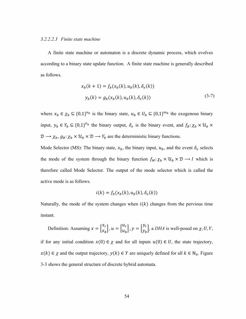
54

3.2.2.2.3 Finite state machine

A finite state machine or automaton is a discrete dynamic process, which evolves

according to a binary state update function. A finite state machine is generally described

as follows.

1 , ,

, , (3-7)

where ∈ ⊆ 0,1 is the binary state, ∈ ⊆ 0,1 the exogenous binary

input, ∈ ⊆ 0,1 the binary output, is the binary event, and :

⟶ , : ⟶ are the deterministic binary functions.

Mode Selector (MS): The binary state, , the binary input, , and the event selects

the mode of the system through the binary function : ⟶ which is

therefore called Mode Selector. The output of the mode selector which is called the

active mode is as follows.

, ,

Naturally, the mode of the system changes when changes from the pervious time

instant.

Definition: Assuming , , , a DHA is well-posed on , , ,

if for any initial condition 0 ∈ and for all inputs 0 ∈ , the state trajectory,

∈ and the output trajectory, ∈ are uniquely defined for all ∈ . Figure

3-3 shows the general structure of discrete hybrid automata.

3.2

wh

and

sub

sys

hie

sys

2.2.3 Mixed

Mixed Log

hich transfor

d continuous

bject to line

stems can be

erarchical fo

stem into two

The MLD o

Fig

d logical dyn

gical Dynam

rm the logic

s variables. T

ar mixed-int

e described

rm for pow

o layers.

of a hybrid s

gure 3-3 Dis

namical syste

mics (MLD)

cs into linear

Thus, MLD

teger inequa

in the MLD

wer systems

system can b

55

crete hybrid

ems

is another

r inequalitie

describes th

alities. A wi

D form. The

studies sinc

be described

d automata [7

design proc

es. These in

he system by

ide range of

MLD form

e there is n

in the follow

78]

cedure for h

nequalities i

y linear dyna

f systems in

m is more su

o need for d

wing general

hybrid system

include integ

amic equatio

ncluding pow

uitable than

decoupling t

l form [79].

ms,

ger

ons

wer

the

the

56

1

(3-8)

where is the discrete time instant, ∈ is the continuous states of the system,

∈ are the inputs and ∈ are the outputs, ∈ 0,1 are the binary variable and

∈ are auxiliary continuous variables which are introduced while translating PWA

functions into linear inequalities. The general MLD form presented in (3-8) contains all

constraints on states, inputs, outputs and auxiliary variables and all the state space

equations of the system. It should be noted that the equality equations, which include the

dynamics of the system in discrete form, are linear equations. However, the nonlinearity

is hidden in the integrality constraints on the binary variables. A combination of a binary

state , binary input , and binary variable is called a mode. If for a given

, , , there exists a ∈ , ∈ and ∈ such that the inequality in (3-8)

holds, the mode is called feasible; else it is infeasible [79], [18]. An MLD representation

of a system is Well-posedness if the following Lemma holds.

Lemma: If for every given pair ∈ and ∈ , the values of and

are uniquely defined by the inequality in (3-8), the MLD model is well-posed.

All the MLDs in this dissertation are considered to be well-posed. It should be noted

that this assumption is not restrictive and is always satisfied when real physical plants

are described in the MLD form [79]. It should also be noted that automata, propositional

logic, if . . . then . . . else statements, and PWA functions can all be described in MLD

form. However, nonlinear functions such as network equations in power systems cannot

be

He

ass

con

con

the

for

can

directly des

ereafter, we

sumption is

nverted to M

nverted to th

A generaliz

e MLD form

rce the system

Although a

n approxima

scribed in M

will mainly

not limiting

MLDs. Tabl

he MLD form

zed stabilizin

m. For exam

m to follow

all the above

ate nonlinea

MLD form a

y consider t

g since a hy

e 3 shows h

m.

Table 3 M

ng controlle

mple, a stabi

a desired ref

e-mentioned

ar systems a

57

and should

the hybrid

ybrid system

how each o

MLD transfo

er can also b

ilizing mode

ference traje

models are

arbitrarily a

be approxim

systems in

m defined in

of the eleme

form [78]

be derived fo

el predictive

ectories is dis

avoid nonlin

accurate. Fu

mated by PW

the form o

n any other

ents of hybr

or the system

e control sc

scussed in [7

near equatio

urther, all of

WA functio

f MLDs. T

form could

id systems

ms described

cheme that c

79].

ons, all of th

f these hyb

ons.

This

be

are

d in

can

em

brid

58

models may include thresholds on states, inputs and internal variables. Also, they may

include binary states that are part of a finite state machine or an automaton. Thus, all of

the aforementioned hybrid system models are equivalent and several programs exist for

systematical transforming to each other [80], [18].

Despite of being equivalent, each of these modeling frameworks has their specific

benefits. DHAs models have separate blocks and are easily understandable by the user,

which makes it more convenient for user interface. MLD models are suitable for online

optimal control and PWA models are suitable offline optimal control [81], to design

observers for hybrid systems [82], and to perform analysis tasks.

As mentioned earlier, direct modeling of hybrid systems in MLD or PWA form is

usually excruciating. Researchers at ETHZ University developed a program called

HYbrid Systems DEscription Language (Hysdel) [83] which allows the designer to

describe a hybrid system on a textual basis. This is very similar to DHA models and

describes the hybrid system in blocks. They also developed a compiler that converts the

input text to PWA and MLD forms, which is basically transforming DHA hybrid system

to PWA and MLD. The Hysdel language has been used to develop most of the models in

this dissertation.

Example1:

100

(3-9)

59

In this case the constraint 0could be assigned to an auxiliary binary variable,

δ k . Therefore, when this switch is on the system is in one state and when it is off the

system is in another state.

δ 1 ↔ 0 (3-10)

According to [79] we have the following general equation.

0 ↔ δ 1 is true if and only if 1

(3-11)

where, M and m are the maximum (or supremum) and minimum (or infimum) or

Thus, assuming that the Maximum and minimum of the x(k) are +10 and -10 (M=+10

and m=-10), (3-10) is equivalent to the following two inequalities.

mδ x m

ε δ ε (3-12)

Then the system’s differential equation (3-9) could be rewritten in the following unique

form.

1 2δ (3-13)

Defining the auxiliary variable δ , we have the following equations.

60

1

1

(3-14)

Example 2:

Consider the following piecewise linear system from [79].

1 0.8cos α sin αsin α cos α

01

1 0 (3-15)

where,

α 31 0 0

3 10 0

∈ 1010 1010

∈ 1 1

(3-16)

Using auxiliary variables k ∈ and δ ∈ 0,1 such that δ k 1 ↔ 10 x k

0 equation (3-15) can be rewritten as follows.

1

Thus in this case we have the following equations for the system in the two cases.

61

1 0.4 0.690.69 0.4

01

↔ 1 0 x k 0

1 0.4 0.690.69 0.4

01

↔ 10 x k 0

(3-17)

where,

0.4 0.690.69 0.4

0.4 0.690.69 0.4

(3-18)

Using the MLD approach discussed earlier,

1

1

(3-19)

Expanding in the matrix form, results in the following.

1010

0000

0 00 0 0

000 0 0

00 00 00 00 0

000000

0011

10100000

00

10

0

00

11

62

where is a small positive scalar, 01 , 1 √3 11 ,

10 11 , and , are obtained from (3-15) by setting , respectively.

3.2.3 Background on the optimization of hybrid systems

An optimization problem could be expressed in the following general form.

min

Subj. to 0 , 1, … , (3-20)

whereξ is the optimization variable which can be defined in the general form of ξ ≜

ξξ . The general form contains the real-valued part ξ and the integer-valued part ξ .

The optimization problem tries to find a vector ξ∗ that minimizes the objective function

such that the inequality constraints fi( ) ≤ 0 hold.

A point is called feasible if it satisfies all the constraints fi( ) and the optimization

problem (3-20) is called feasible if there exists at least one feasible point in the input

domain. The set of all feasible inputs is referred to as the feasible set. The optimal value

∗ of the problem (3-20) is defined as follows.

∗ inf | 0; 1, … , (3-21)

The solution to the optimization problem from the feasible set of inputs, ∗, is

referred to as the optimizer. The optimizer is called a local optimizer if it minimizes the

cost function in a subset of the feasible set and a global optimizer if it minimizes the cost

for the whole feasible set.

63

If the objective function and the inequality constraints in optimization problem

(3-20) are convex and no binary variables are present in the optimization variable the

problem is referred to as a convex optimization problem. In a convex optimization

problem the feasible set is convex, and any locally optimal point is also globally optimal.

If the objective function and constraints of the optimization problem (3-20) are

linear, the problem is referred to as a Mixed Integer Linear Programming (MILP)

problem, which can be expressed as follows.

min

Subj. to

(3-22)

where G is a matrix and c and g are row vectors. Although the objective function and

constraints are linear, the optimization problem is not convex due to the existence of

integer variables. Thus locally optimal points are not necessarily globally optimal.

Further, MILPs are NP-hard which means the solution time grows exponentially with the

number of binary variables [84].

Several algorithms have been proposed to solve MILP problems including branch

and bound, cutting plane, decomposition and logic-based methods. Details of these

algorithms could be found in [85]. Obviously, if the optimization vector contains only

real and no integer components, problem (3-22) reduces to a Linear Program (LP),

which is convex which means a local minimize to the problem is in fact the global

minimize and the problem can be solved in polynomial time. Similarly, the Mixed

Integer Quadratic Programming (MIQP) problem can be formulated as follows.

64

min12

Subj. to

ξ ≜ξξ , ξ ∈ , ξ ∈ 0,1

(3-23) (3-24)

where Q is a weight matrix.

Mixed integer programming problems are classified in general as NP-hard, which

means that with the available algorithms in the worst case, the solution time grows

exponentially with the number of integer variables [84].

In this dissertation, the objective function is defined to penalize the predicted

evolution of the state, control input and output over the finite horizon N using a norm.

Also the weight matrices and Q are always defined to be full column rank matrices. The

prediction is performed using the MLD model of the system at every time-step within

the prediction horizon which means the MLD model is augmented for N steps to predict

the behavior of the system ahead of time.

If the MIQP problem is solved subject to the MLD model of the system the

optimization vector can be written as follows.

0 , … , 1 , 0 , … , 1 , 0 , … , 1 (3-25)

where , , are the vectors of continuous, discrete and auxiliary variables, respectively.

As can be seen in (3-25), the optimization vector includes discrete and continuous

variables.

65

The control input at time-instant k is obtained by minimizing the objective function

subject to the evolution of the MLD model and its mixed-integer linear inequality

constraints. This yields to Constrained Finite Time Optimal Control (CFTOC) problem

which can be expressed as follows.

∗ argmin ,

Subject to MLD model (3-26)

Furthermore, additional integrality constraints are present on the binary variables

and on binary inputs. Solving this problem yields a sequence of optimal control inputs

∗ , … , 1 . If a linear norm is used in the cost function of

(3-31), the CFTOC problem leads to solving an MILP and if a quadratic norm is used, it

leads to solving MIQP, respectively.

Several algorithms have been proposed and applied successfully to medium and

large size application MIQP problems [86], the four major ones being:

Cutting plane methods, where new constraints (cuts) are generated and added to

reduce the feasible domain until the optimal solution is found

Decomposition methods, where the mathematical structure of the models is

exploited via variable partitioning, duality, and relaxation methods

Logic-based methods, where disjunctive constraints or symbolic inference

techniques are utilized, which can be expressed in terms of binary variables

Branch and bound (B&B) methods, where the 0-1 combinations are explored

through a binary tree, the feasible region is partitioned into sub-domains

66

systematically, and valid upper and lower bounds are generated at different levels

of the binary tree.

More details and analysis of the multi of multi-parametric programming for MILPs

and MIQPs could be found in [87],[88],[89]. In this dissertation, branch and bound

method is used for solving the MILP/MIQP problem and will be discussed in more detail

in section 3.3.1.

3.2.4 Dynamic Reactive Power Control of Power Systems

The objective of reactive power control is to minimize losses and to keep the bus

voltages within limits while satisfying all system constraints. As mentioned earlier,

cables are usually short in isolated power systems; therefore, minimizing loss is not be

the best option as the objective function in these systems. In this case, a better candidate

is the sum of voltage deviations of critical buses in the system. It should be noted that

when the total voltage deviation is minimized, the total loss of the system is minimized

indirectly. Reactive power control of an isolated power system can be formulated in the

following general form.

min ,.. , ,…, , , (3-27), , (3-28)

, , , 0 (3-29), , 0 (3-30)

The cost function given by (3-27) can be chosen to minimize the voltage deviation of

the buses that are more likely to have voltage drop, i.e., load buses. In this problem, the

cost function is chosen to minimize the voltage deviation over a prediction horizon on N.

67

The prediction horizon and step size is chosen by the operator to cover the slowest

dynamic of the system and not to exceed the maximum possible computation time for

online control. Hence, assuming the current time instant as t0, the voltages of the critical

buses of the system should be predicted over the horizon of N to calculate the cost

function. The control action should also be included in the cost function to reduce the

possibility of having too much control action which may result in actuator aging and

damage in the system. Thus, the objective function (3-27) could be written as follows.

, , |

,∈

⋯

… ‖ ∆ ‖ , ‖ ∆ ‖ ,

(3-31)

In (3-31), is the set of the buses which are more important for voltage control, i.e.,

the buses that are close to the loads, N is the horizon of the optimization, W1 and W2 are

user definable input weight matrices and | is the phasor of estimated voltage

of bus i at the time +k based on the bus voltage measurement at time .

As shown in (3-28) and (3-29), the optimization problem is subject to the following

simplified and discretized differential algebraic equations.

1 Δ1

,

1

(3-32)

68

1 Δ1

,,

1

, , 2, … ,

(3-33)

1 Δ

, 1, … ,

(3-34)

N

jjnnjjnnjjnn

N

jjnnjjnnjjnn

kkBkkGkVkVkQ

kkBkkGkVkVkP

1

1

))()(cos())()(sin()()()(

))()(sin())()(cos()()()(

(3-35)

where is the number of DGs and is the number of dynamic loads. The DAE

equations (3-32) through (3-35) are simplified DAE equations of the sources and loads

and the network equations of the system. Equation (3-32) represents the dynamics of the

master generator; (3-33) the dynamics of PQ controlled DERs and (3-34) the dynamics

of the loads and (3-34) are the network equations. In (3-36), ∑ is the sum of the

reactive power injected and withdrawn from bus n as follows.

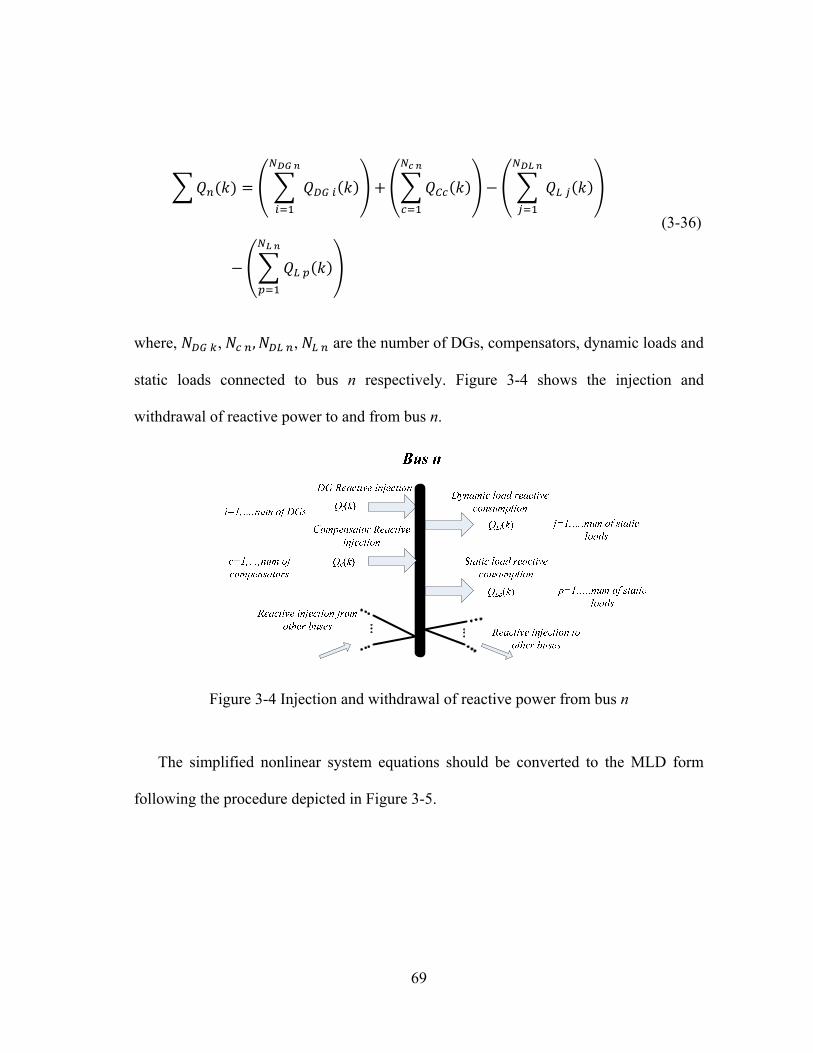
69

(3-36)

where, , , , are the number of DGs, compensators, dynamic loads and

static loads connected to bus n respectively. Figure 3-4 shows the injection and

withdrawal of reactive power to and from bus n.

Figure 3-4 Injection and withdrawal of reactive power from bus n

The simplified nonlinear system equations should be converted to the MLD form

following the procedure depicted in Figure 3-5.

70

Figure 3-5 Converting the system to MLD form

Equations (3-29) and (3-30) include the bus voltage limits, compensator limits, cable

thermal limits and power equality of the system given by following equations:

| | 1, … . ,

1, … , | | 1, … ,

(3-37)

where NBus is the number of buses, NComp is the number of compensators and Ncl is the

number of the cables, | | is the voltage magnitude of bus b at time , reactive

power setpoint of compensator c at time and | | is the current of cable cl at time k.

The thermal rating of an overhead line is the maximum current that the line can handle

without overheating and it is highly dependent on the conductor and insulator materials

and the working condition.

Figure 3-6 shows the prediction of the voltages in the system using the model (3-32)

through (3-35). This figure shows the predicted voltage profile of two buses in the

system over a horizon of N with step time of k. The objective of model predictive control

is to select a control sequence force the voltage to follow the reference voltage profile. In

the voltage and reactive control of the isolated power system, the main goal is to make

71

the bus voltages achieve the nominal voltage value which is usually constant and equal

to 1 per unit.

Figure 3-6 Prediction of the voltage profile of buses in the system for MPC

Hypothetically, if the system has only one control input, the control sequences

discussed in Figure 3-6 may look like Figure 3-7.

72

Figure 3-7 Sequence of control inputs

By combining Figure 3-6 and Figure 3-7 Sequence of control inputsFigure 3-7,

Figure 3-8 show the concept of model predictive control with a discrete prediction of

voltage over the horizon N.

Figure 3-8 General concept of model predictive control

74

In (3-28), x(k) is the vector of the state space variables as follows.

… … …

2,… , , 1,… ,

(3-38)

where NDG is the number of DGs and NLoad is the number of loads, is the state

variable of the master generator which is numbered as the first DG, is the state

variable of the i'th DG, is the reactive power state variable of j’th load.

In (3-28), the control variables in the v(k) vector can include voltage and reactive

power of generators, Generated reactive power of compensators. Some or all of these

inputs may be used in the reactive power control based on the studied power system and

based on the needs. Thus, v(k) which is the vector of continuous control inputs is defined

as follows.

, , … … 2,… , , 1,… ,

(3-39)

where , is the reference voltage of the master generator and , is

the reference reactive power injection of i’th DG, is the reactive power reference

of c’th dynamic compensator if dynamic compensators are present in the system. is

the vector of the discrete control inputs to the system, i.e., … where

NSW is the number of controllable discrete inputs in the power system. The augmented

control vector u(k) is defined as the augmented vector of discrete control and

continuous control inputs, i.e. u(k)= . Figure 3-10 shows the process of

calculation of the objective function in (3-31).

75

Network equation

Objective function

V1(k)

Pi(k), Qi(k)

PLj(k), QLj(k)

Master generator

1 1 1 Δ1

1 , 1

PQ mode DGs

Dynamic loads

1 Δ1

,,

1 Δ

0

i=1,…, num of PQ DGs

j=1,…, num of dynamic loads

N

jjnnjjnnjjnn

N

jjnnjjnnjjnn

kkBkkGkVkVkQ

kkBkkGkVkVkP

1

1

))()(cos())()(sin()()()(

))()(sin())()(cos()()()(

PL k(k), QL k(k)

Qc(k)

xj(0)

xi(0)

x1(0)

Figure 3-10 Process of calculation of the objective function

76

In the next part we will discuss how we derived the simplified differential equations

defined by (3-28), the algebraic equations defined by (3-29). The differential constraints

of the system expressed in (3-28) include the dynamics of the generators and the loads in

the power system. These equations are usually expressed in continuous time domain and

then discretized and linearized. First of all, we discuss the dynamics of the sources in

time domain. Then we will discuss how we simplified and discretized the equations for

reactive power control.

3.2.4.1 Sources

Generators should be modeled with appropriate amount of detail for the study. For

synchronous generators, the model should include automatic voltage regulator, exciter,

turbine and governor [90], [91]. Model of the synchronous generator can be significantly

simplified by neglecting stator dynamics and the decrease in accuracy of the model is

negligible with such simplification. Hence, neglecting generators stator dynamic is very

common in the literature [91]. Following equations model the synchronous generator

rotor dynamics and exciter dynamics in continuous time domain.

77

2

(3-40)

:rotor angle (radian)

:rotor speed (radian per second)

:exciter voltage on stator base (p.u.)

( ): quadrature (direct) axis transient voltage (p.u.).

:stator q-axis(d-axis) component of currents (p.u.)

, :bus voltage magnitude and angle respectively.

, :direct axis synchronous, transient and sub-transient reactance (p.u.)

respectively.

, :quadrature axis synchronous, transient and sub-transient reactance (p.u.)

respectively.

78

:direct axis open circuit transient and sub-transient time constants (seconds)

respectively.

:quadrature axis open circuit transient and sub-transient time constants (seconds)

respectively

Also , , are the exciter gains.

Stator algebraic equations are written as follows.

sin 0

cos 0 (3-41)

where is the stator resistance. In order to derive the network equations, we have to

compute the generated active and reactive power of the generator. The generated active

power equations are as follows.

, sin cos ,

1, … , (3-42)

where is the phase of bus i. The generated reactive power by this generator is

calculated as follows.

, cos sin ,

1, … , (3-43)

Generators have some physical constraints on the amount of reactive power that they

can produce or consume. The reactive capability limits of the generator should be

considered in dynamic reactive control studies. The continuous reactive power output

79

capability is limited by three constraints [90]: the armature current limit, the field

current limit, and the end-region heating limit.

Although the model presented in (3-40) to (3-43) may be used as the plant model in

reactive studies, using this model as the prediction model makes the computational time

of the optimization too long. Thus, the full model may not be used for prediction and

simplifications should be applied. We used system identification methods to achieve a

simple model of the component that can be used in the prediction model in this research.

Since mainly the output voltage of the master generator is important in volt/Var studies,

the model should describe the change in output voltage as a result of a change in the

input voltage reference. Hence, an input-output model with the reference voltage as the

input and estimates the output voltage is enough as the prediction model. In this

research, a first order model which is derived based on the step response of the voltage is

used as the prediction model for the master generator.

,

11

(3-44)

where is the time constant which is identified with system identification. For the

master DG, the simplified state space equations can be derived by transferring (3-44)

into the state space form as follows.

1,

1

(3-45)

80

If more accuracy is needed, especially for small systems with limited number of DGs, a

2nd order model could be used to estimate the voltage. The general form of the 2nd order

model is as follows.

, 2

(3-46)

The discretization can be performed using the following formula.

1∆

(3-47)

Example:

The master generator state space equation (3-48) can be discretized using (3-47) as

follows.

1 Δ1

, (3-48)

Figure 3-11 shows the actual generator voltage response and the estimated voltage

using 1st and 2nd order models for a step of 0.05 p.u. in the reference voltage of the

synchronous generator.

81

Figure 3-11 Actual synchronous generator voltage and estimated voltage using 1st and 2nd order models

As can be seen in Figure 3-11, the actual response of the generator is smaller than the

reference due to saturation and system dynamics; however, the identified model can be

adjusted by adding an extra gain on the identified model. Figure 3-12 shows the

schematic diagram of a typical controller for DFIG wind generator.

Figure 3-12 Schematic diagram of conventional control of DFIG wind generator

1.5 2 2.5 3 3.5 4 4.5 50.98

1

1.02

1.04

1.06

1.08

Time(s)

Vo

ltag

e (

p.u

.)

Actual generator voltage1st order estimation2nd order estimation

82

The dynamic equations are obtained from Newton’s equations of motion for each

mass (rotational speed) and shaft (torsion or twist angle) [92].

2

1

2

(3-49)

(3-50)

(3-51)

where ωt and ωr (p.u.) are the turbine and generator speeds, respectively; θtw (rad) is the

shaft twist angle; Ht and Hg (sec) are the turbine and generator inertias, ωelB (rad/s) is the

electrical base speed, Pt (p.u.) is the turbine input power, and Tsh and Te (p.u.) are the

shaft and generator torques which are defined as follows.

(3-52)

where k (p.u./el.rad) and c (p.u.s/el.rad) are the shaft stiffness and damping coefficients.

In this dissertation, the dynamic equations of the DFIG are described in the dq frame

with the d-axis leading. First, following variables are defined.

83

(3-53)

where and (p.u.) are the rotor q- and d fluxes, Rr (p.u.) is the rotor resistance,

Kmrr = Lm/Lrr and Lss, Lrr, and Lm (p.u.) are the stator, rotor, and mutual inductances,

respectively.

For balanced and unsaturated conditions, the corresponding p.u. DFIG model is as

follows.

1

1

1

1 1

1 1

1

(3-54) (3-55) (3-56) (3-57)

where iqs and ids (p.u.) are the stator q- and d-axis currents, ωs (p.u.) is the synchronous

speed, ωel = ωelB ωs, Rs (p.u.) is the stator resistance, and R1 = Rs + R2 and .

84

The generator dynamic equations could be divided into three parts: stator electrical

(3-54), (3-55); rotor electrical (3-56), (3-57) and rotor mechanical (3-51). Similar to

synchronous generator, stator transients are neglected without losing accuracy [90]. The

ac voltage of the rotor-side converter is dependent on the control objectives of the wind

generator. The grid side converter is responsible for controlling the capacitor voltage

which is equivalent to sending the maximum active power to the grid and also reactive

power control. The controller is usually designed in the converter dq-axis with

decoupled control on real and reactive power. The rotor side control is not of interest in

this dissertation and more details could be found in [93].

The active and reactive power sharing between the wind generator and the network

could be written as follows.

sin

cos

(3-58)

Figure 3-13 shows schematic diagram of a typical controller of photovoltaic source [94],

[95].

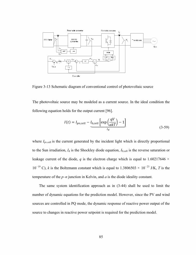
85

Figure 3-13 Schematic diagram of conventional control of photovoltaic source

The photovoltaic source may be modeled as a current source. In the ideal condition the

following equation holds for the output current [96].

, , exp 1 (3-59)

where Ipv,cell is the current generated by the incident light which is directly proportional

to the Sun irradiation, Id is the Shockley diode equation, I0,cell is the reverse saturation or

leakage current of the diode, q is the electron charge which is equal to 1.60217646 ×

10−19 C), k is the Boltzmann constant which is equal to 1.3806503 × 10−23 J/K, T is the

temperature of the p–n junction in Kelvin, and a is the diode ideality constant.

The same system identification approach as in (3-44) shall be used to limit the

number of dynamic equations for the prediction model. However, since the PV and wind

sources are controlled in PQ mode, the dynamic response of reactive power output of the

source to changes in reactive power setpoint is required for the prediction model.

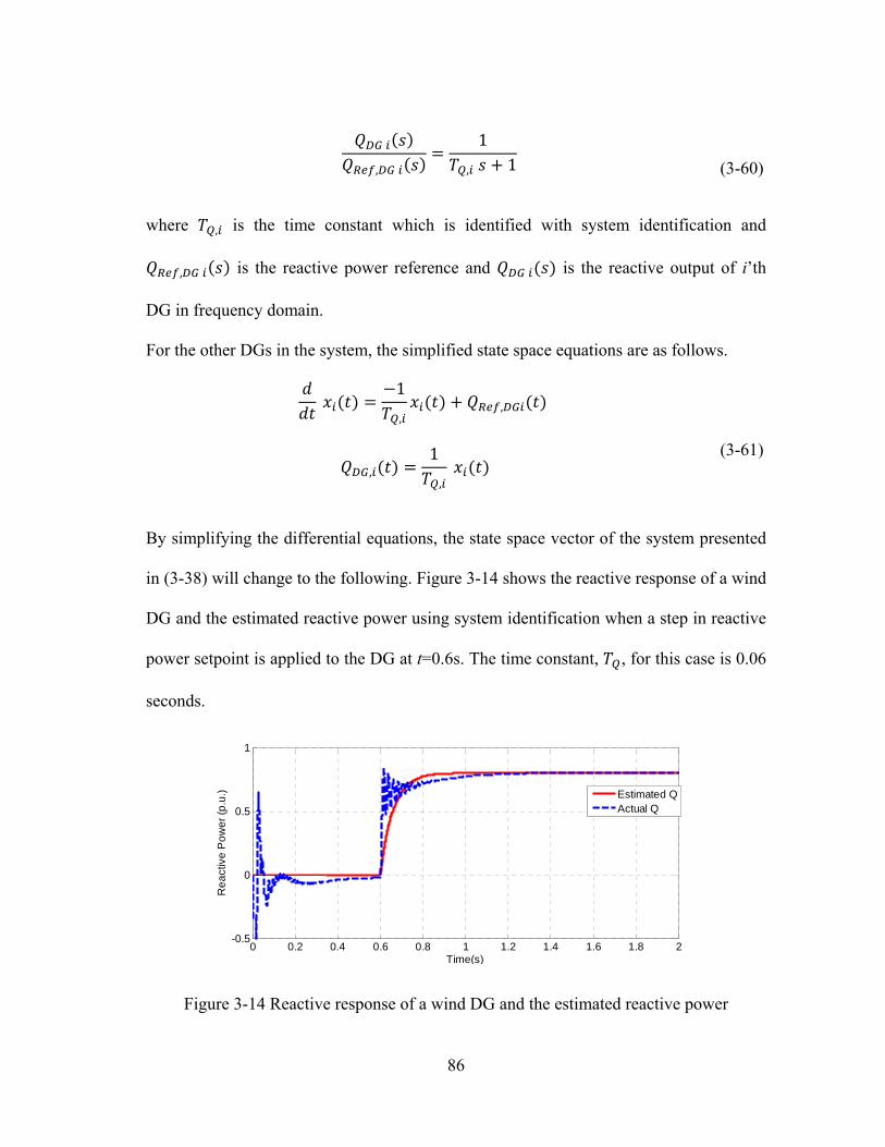
86

,

1

, 1

(3-60)

where , is the time constant which is identified with system identification and

, is the reactive power reference and is the reactive output of i’th

DG in frequency domain.

For the other DGs in the system, the simplified state space equations are as follows.

1

,,

,1

,

(3-61)

By simplifying the differential equations, the state space vector of the system presented

in (3-38) will change to the following. Figure 3-14 shows the reactive response of a wind

DG and the estimated reactive power using system identification when a step in reactive

power setpoint is applied to the DG at t=0.6s. The time constant, , for this case is 0.06

seconds.

Figure 3-14 Reactive response of a wind DG and the estimated reactive power

0 0.2 0.4 0.6 0.8 1 1.2 1.4 1.6 1.8 2-0.5

0

0.5

1

Time(s)

Re

act

ive

Po

we

r (p

.u.)

Estimated QActual Q

87

… … …

2,… , , 1,… , (3-62)

where is the state of the master generator, ’s are states of the other sources and

are the states of the loads.

3.2.4.2 Loads

The power consumed by most of the loads in a power system is voltage dependent.

Hence, the load admittance varies dynamically with the voltage which means that when

the voltage decreases the consumed power of most of the loads decrease. However, after

the disturbance, internal controllers of the most of the loads like thermostats of electrical

heating and power electronics converters which regulate the rotational speed of

machines restore the power demand of the load. The new power demand usually settles

usually below or equal to the pre-disturbance level. This self restoring behavior of the

load can be described using second order differential equations as described in [73],

[97], [98]. One set of equations model the active power and another set model the

reactive power of the load [99].

(3-63)

In (3-63), is an internal state variable which models the load recovery

dynamic of the j’th load with the time constant Tpj. The instantaneous voltage

88

dependency is expressed by Vat and the steady-state voltage dependency is given by Vas.

In this model, the actual active power PL can be considered as an output, the absolute

value of the load voltage V is the input and PL0 j is the rated active power of the load.

Similarly, the load model for the reactive power is defined as follows.

(3-64)

where QL0 j is the rated reactive power of the of the j’th load and is the actual

reactive power of the j’th load at time t and Tq j is the load reactive recovery time

constant of the j’th load. Figure 3-15 shows the currents and the voltages of the load.

Figure 3-15 Load current and voltage

Linearizing (3-64) around the operating point of the system yields to the following.

∗ ∗ (3-65)

89

where, ∗ is the operating voltage of the bus connected to the j’th load. Mathematical

manipulation of (3-65) yields the following linear transfer function.

∆ 1

∆ (3-66)

where the matrices and are defined as follows.

∗

,∗

(3-67)

where is the nominal bus voltage and ∗ is the operation point of the bus voltage.

It is important to take into account the high reactive power consumed by the motor in

the startup [100]. In such a case, the rating of the upstream equipment may need to be

rated higher than the steady-state condition and some adaptation should be performed on

the controller to alleviate the voltage drop as much as possible [101]. The amount of the

voltage dip caused by motor startup is directly related to reactive power need of the

motor load during startup. The typical value of the power factor for motors under 1000

HP is about 0.20 [102]. The locked rotor kVA per HP is defined for each NEMA code

letter (Appendix A) which can be used to determine the expected startup reactive power

need of the motor [103].

In addition, large squirrel-cage induction motors and industrial synchronous motors

draw several times their full load current from the supply causing a power factor in the

range of 0.15–0.30 lagging during their startup. The actual shape and magnitude of the

staring current curve depends on the voltage at the motor terminals, the motor design,

and the characteristic of the load which is connected to the motor [104].

90

3.2.4.3 Network equations for balanced microgrid

The algebraic equations include the network equations of the power system. Network

equations can be expressed in either power balance or current balance form. The current

balance from is more common in software packages. Figure 3-16 shows the connection

of synchronous generator to the rest of the network.

Figure 3-16 Connection of synchronous generators and the rest of the network

In this section, we derive the network equations for balanced and unbalanced

networks. If the net apparent power injection into the bus n is defined as Sn=Sgn-Sdn , we

can express Sn as follows.

)()()( * tItVtS nnn (3-68)

where Vn is the phasor of the voltage of the bus Vn(t)=|Vn(t)|n assuming that the

voltages are balanced. Ik is net of the injected current into the bus n which can be

expressed as follows.

91

)()(1

tVYtI j

N

jnjn

(3-69)

where, Ynj are the admittance matrix elements and Vj ’s are voltages of the buses.

Substitution of (3-69) into (3-68) yields to the following equation.

)()()()()( *

1

*

*

1

tVYtVtVYtVtS j

N

jnjnj

N

jnjnn

(3-70)

If the system is balanced, Ynj which is a complex number can be expressed as

Ynj=Gnj+jBnj where Gnj is the real part and Bnj is the imaginary part of the admittance

matrix element Ynj. Given that Sn(t) =Pn(t)+jQn(t), we can express (3-70) as two

equations, one for the real power, Pn, and one for the reactive power, Qn(t), as follows:

N

jjnnjjnnjjnn

N

jjnnjjnnjjnn

ttBttGtVtVtQ

ttBttGtVtVtP

1

1

))()(cos())()(sin()()()(

))()(sin())()(cos()()()(

(3-71)

The two equations of (3-71) are referred to as power flow equations. Obviously,

power flow equations are nonlinear, thus, they need to be linearized in order to be used

in the hybrid control scheme. The power flow equations are very complex and are

functions of many variables. Thus piecewise linear approximations of any one variable

will depend on the value of the other variables. Thus, we seek to simplify the equations

based on some observation of the power system.

The resistance of the cables in power system is usually significantly less than the

reactance and the x/r ratio is often between 2 and 10. Further, in most of shipboard

92

power system and MicroGrid applications, the cables are fairly short. Also, angle

difference between buses in power systems is directly coupled with the active power

flow of the system. Usually, the difference between the voltage angle of the adjacent

buses which are connected by a cable is less than 10-15 degrees [105]. It is extremely

rare to ever see such angular separation exceed 30 degrees. Figure 3-17 confirms this

observation for a MicroGrid which encounters heavy loading and loads changes. As can

be seen in Figure 3-17, most of the angles are small and do not experience significant

changes during different load conditions of the MicroGrid.

Figure 3-17 Bus angles for a MicroGrid for a case-study with changing loads

0 1 2 3 4 5 60

2

4

Th

eta

1 (

de

g)

0 1 2 3 4 5 60

5

Th

eta

2 (

de

g)

0 1 2 3 4 5 60

10

20

Th

eta

3 (

de

g)

0 1 2 3 4 5 60

10

20

Th

eta

4 (

de

g)

0 1 2 3 4 5 60

5

Th

eta

5 (

de

g)

0 1 2 3 4 5 60

10

20

The

ta7

(de

g)

0 1 2 3 4 5 60

5

10

Time(s)

Th

eta

7 (

de

g)

93

This observation can help us to eliminate the trigonometric functions in (3-71)

considering the fact that the angular difference across the cables only appears as the

argument of the trigonometric functions sine and cosine.

3.2.4.4 Network equations for unbalanced microgrid

Single phase load connected to the buses of the power system or distributed along

the lines are the main reason of imbalance in the distribution system. Further, single-

phase loads may vary significantly during different times of the day or week, or season

[106]. Also, operation of fuses may cause a significant amount of load to be

disconnected from the system and substantially increase system imbalance. Large

voltage imbalance (>3%) results in high ripple currents on the dc bus of the three-phase

inverter-based DERs. These ripples in the current may have a degrading effect on the

inverter and the energy sources [106]. It should also be noted that most rotating

equipments, specifically generators, are designed to operate with no more than as

specified current imbalance (ANSI/NEMA MG 1- 2006). Further, imbalances in the

distribution system or load imbalance can cause negative sequence currents. Three-phase

DERs and motors have limited negative sequence capability and may be damaged by

imbalanced load conditions but the damage can be minimized by the use of a negative

sequence current relay. The maximum allowed continuous voltage unbalance in the

distribution system is 5% according to NEMA MG1.

It should also be mentioned that in power systems, most voltage unbalance

conditions are due to magnitude inequalities while the phase-angles are equal (120° or

2π/3) or nearly equal [1]. If the voltage unbalance is in this category and the inequalities

94

in the magnitudes is less than 1%, the DER with an inverter interface can compensate for

the voltage unbalance by providing different amounts of reactive power on each phase.

This local control scheme is beyond the scope of this dissertation and the interested and

the interested reader is referred to [1] for more information.

The objective function and power flow equations of the formulation in previous section

should be changed for the unbalanced power system.

, , |, ,

∈

|, ,

|, ,

‖ ∆ ‖ , ,

‖ ∆ ‖ , ,

(3-72)

where | , | , | are the predicted voltage of phase

A, B and C of bus i, respectively.

The problem is solved subject to differential equations of the sources and loads

(3-32), (3-33), (3-34), and the constraints of the system (3-37) and the network

equations. The network equations for the unbalanced system are solved in an iteration

fashion and each iteration is as follows. A ladder iterative technique can be used to solve

the unbalanced power flow [107] , [108]. The power flow equations are as follows for

two adjacent nodes.

(3-73)

95

Figure 3-18 shows the structure of two adjacent nodes n, m in the power system.

Figure 3-18 A series feeder component

In this formulation the loads and PQ generators should be converted to current as

follows.

∗

(3-74)

The interested reader is referred to [107] for more information about the iterative

distribution power flow. Figure 3-19 shows the process of calculation of the objective

function in this case.

96

1 1 1 Δ1

1 , 1

1 Δ1

,,

1 Δ

0

∗

∗

Figure 3-19 Process of calculation of the objective function

97

In the next part, we will discuss modeling of all the elements in the unbalanced

power systems, which are used in the unbalanced power flow.

3.2.4.4.1 Lines

The series impedance of a line section l is represented by a 3×3 matrix [109], [107]:

, , ,

, , ,

, , ,

(3-75)

3.2.4.4.2 Loads

Loads in power system can be modeled as constant current, constant power and

constant impedance and either one can be Y-connected or Δ-connected. Assuming that

load Li is connected to bus i, Vi is the three-phase voltage in bus i, ILi is three phase load

current, then following load models can be used in the distribution power flow [108]:

1) Grounded-Y, constant power load

∗

(3-76)

where,

, 0 00 , 00 0 ,

(3-77)

2) Grounded-Y, constant current load

98

, , , (3-78)

3) Grounded-Y, constant impedance load

(3-79)

where,

, 0 00 , 00 0 ,

(3-80)

4) Ungrounded-Δ, constant power

∗

(3-81)

where,

1 1 00 1 11 0 1

,, 0 00 , 00 0 ,

(3-82)

5) Ungrounded-Δ, constant current

(3-83)

where , , , .

6) Ungrounded-Δ, constant impedance

, , , (3-84)

where,

3.2

mo

3.2

rep

and

or

3.2

mo

2.4.4.3 Shun

Similar to

odeled exactl

2.4.4.4 Tran

A general

presents prim

d Zt represen

All types o

Y0-Y0 transfo

2.4.4.5 Dist

Distributed

ode. If the u

00

nt capacitors

loads, shun

ly the same a

nsformers

three-phase

mary voltage

nts leakage im

of three-phas

ormer can be

ributed ener

d energy sou

unit is opera

, 00 ,

0 0

s

nt capacitors

as Y or Δ con

e transform

e, Vs represe

mpedance.

Figure 3-2

se transform

e modeled in

rgy sources

urces are cla

ating in PQ

99

00

,

,

can be Y c

nnected con

mer model i

ents seconda

20 Transform

mers, such as

n this framew

assified as P

mode, the

connected or

nstant impeda

is shown in

ary voltage,

mer model

Δ - Y0 trans

work [110].

Q or PV dep

unit model

,

,

,

r Δ connect

ance load, re

n Figure 3-

Ym represen

sformer, Y -

pending on

is identical

(3-

ted and can

espectively.

-20, where

nts core loss

Δ transform

their operati

l with const

-85)

be

Vp

ses,

mer

ion

ant

100

power load, except that the current is being injected into the bus instead of being drawn

from the bus. However, if the unit is in PV mode, the connected bus is modeled as a PV

bus. In this case, if the computed reactive power generation is out of the reactive

generation limits of the unit, then the node can no longer be modeled as a PV bus. Thus,

the unit acts as a PQ unit and the reactive power generation of the unit is set to the

maximum limit.

The unbalanced power flow (3-73) needs to be solved iteratively until the voltages

and currents converge to the solution. The iterative power flow takes a large amount of

computation time even for the static system analysis. Further, the power flow should be

solved by the optimization and control algorithm. Thus, we seek to find a linear relation

between the variables of the power system and the bus voltages. The linear relation can

be introduced by sweeping each of the power system variables in their complete possible

range. The sweeping of the parameters can be performed individually which means for

example can be swept from 0.95 to 1.05 and the sensitivity of the bus voltages

of the system are calculated to a change in . If for example the linearization

yields to two sections for for a bus voltage of bus m, then we have the following

two equations.

0.95 0.95 0.95 1.02 1.02 1.02 →

,

1.02 1.02 1.02 1.05 1.05 1.05 →

,

(3-86)

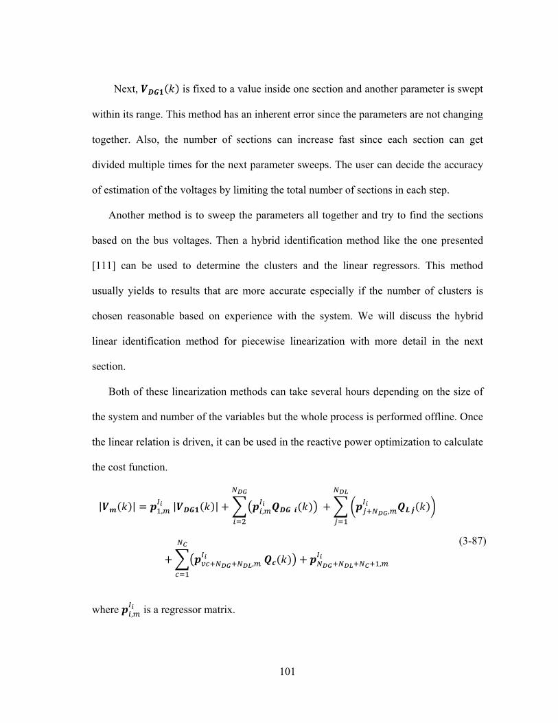
101

Next, is fixed to a value inside one section and another parameter is swept

within its range. This method has an inherent error since the parameters are not changing

together. Also, the number of sections can increase fast since each section can get

divided multiple times for the next parameter sweeps. The user can decide the accuracy

of estimation of the voltages by limiting the total number of sections in each step.

Another method is to sweep the parameters all together and try to find the sections

based on the bus voltages. Then a hybrid identification method like the one presented

[111] can be used to determine the clusters and the linear regressors. This method

usually yields to results that are more accurate especially if the number of clusters is

chosen reasonable based on experience with the system. We will discuss the hybrid

linear identification method for piecewise linearization with more detail in the next

section.

Both of these linearization methods can take several hours depending on the size of

the system and number of the variables but the whole process is performed offline. Once

the linear relation is driven, it can be used in the reactive power optimization to calculate

the cost function.

| | , | | , ,

, ,

(3-87)

where , is a regressor matrix.

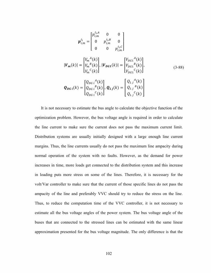
102

,

,, 0 0

0 ,, 0

0 0 ,,

| | , | | ,

,

(3-88)

It is not necessary to estimate the bus angle to calculate the objective function of the

optimization problem. However, the bus voltage angle is required in order to calculate

the line current to make sure the current does not pass the maximum current limit.

Distribution systems are usually initially designed with a large enough line current

margins. Thus, the line currents usually do not pass the maximum line ampacity during

normal operation of the system with no faults. However, as the demand for power

increases in time, more loads get connected to the distribution system and this increase

in loading puts more stress on some of the lines. Therefore, it is necessary for the

volt/Var controller to make sure that the current of those specific lines do not pass the

ampacity of the line and preferably VVC should try to reduce the stress on the line.

Thus, to reduce the computation time of the VVC controller, it is not necessary to

estimate all the bus voltage angles of the power system. The bus voltage angle of the

buses that are connected to the stressed lines can be estimated with the same linear

approximation presented for the bus voltage magnitude. The only difference is that the

103

bus angle is usually coupled with the active power of the loads and generators and has

small coupling with bus voltage magnitude.

3.2.5 Piecewise Linearization

The voltages of the buses in the system can be derived following the piecewise

linearization technique discussed in [111]. Figure 3-21 depicts the piecewise

linearization algorithm which starts with classification of data points into s modes [112].

Then a min squared error algorithm is used to estimate linear hyperplanes that fits the

data points. The number of modes, s, is provided as an estimate by the user based on the

data points to achieve maximum accuracy. The algorithm presented in [111] estimates

the regions, ’s with linear borders.

The state space equations of the power system could be presented in the piecewise linear

form as follows.

1

if , ∈

⋮

if , ∈

(3-89)

Equation (3-89) is referred to as piecewise linear dynamic equations of the system. The

general piece-wise linear time-invariant dynamic system can be described as follows

[79].

Figure 3-221 Sample reesult of class

104

a)

b)

c)

sification alggorithm on 22 dimension

data [112]

105

1 1

⋮ 1

(3-90)

where ∈ 0,1 , are 0-1 variables which satisfy the following exclusive-or

condition.

⨁ 1 (3-91)

Assuming is a bonded polytope, system (3-90) is completely well-posed if and only if

can be partitioned into s non-overlapping parts such that the union of the partitions is

equal to as follows.

∩ ∅, ∀

∪ = (3-92)

Note that assuming that is bounded polytope is not restrictive for power systems

because continuous inputs and states are usually bounded by physical reasons in a power

system, and logical input/state components are intrinsically bounded. The ’s are

defined as follows.

1 ↔ (3-93)

Several nonlinear models can be approximated by a model of the form (3-90),

although this approximation capability is limited for computational reasons by the

number s of logical variables.

106

Knowing that the sets are polytopes of the form : , (3-93)

could be rewritten as follows.

0 ↔ (3-94)

where denotes the jth row of . Equation (3-94) is not easy to solve; however, solving

this equation is equivalent to solving (3-91) and (3-92).

∗ 1

1 (3-95)

where, ∗ ≜ Max ∈ . Equation (3-90) can be rewritten as

follows.

1 (3-96)

Equation (3-96) is nonlinear and involves multiplication between logical variables,

states, inputs. However, we can translate (3-96) into equivalent mixed-integer linear

inequalities. We can start by the following change of variables.

1 ∑ , (3-97)

And let’s define the following min and Max … , …

vectors as follows.

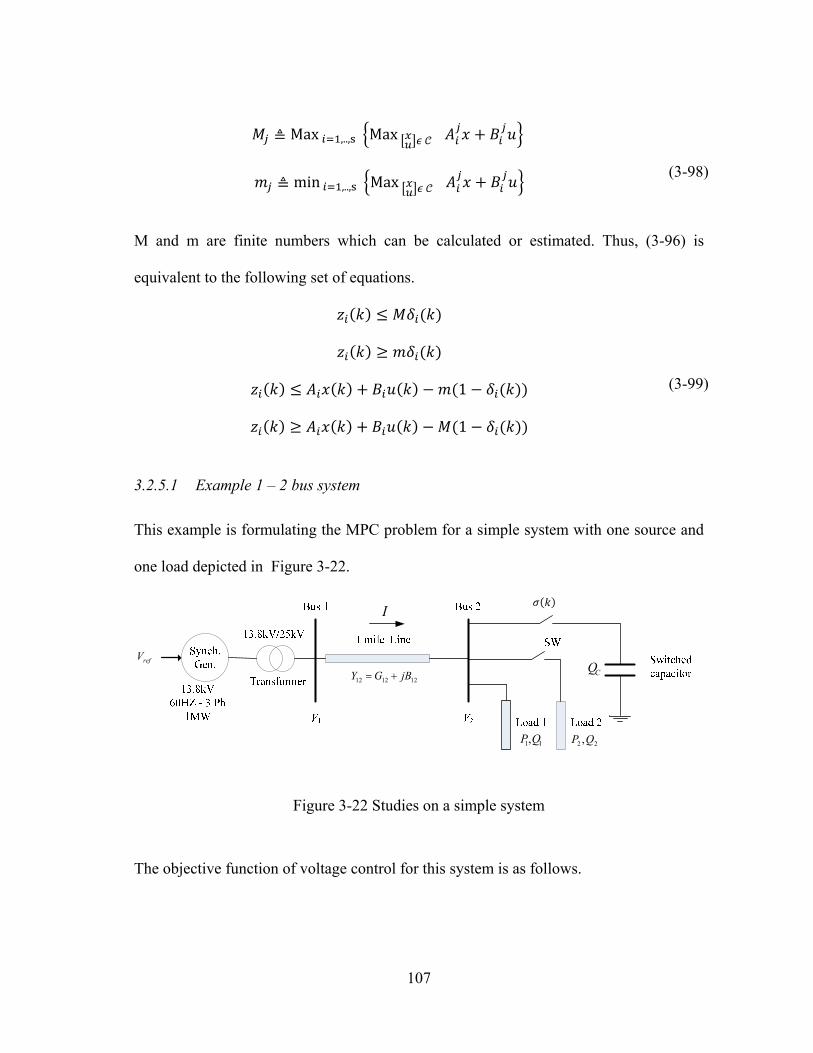
107

≜ Max ,.., Max

≜ min ,.., Max (3-98)

M and m are finite numbers which can be calculated or estimated. Thus, (3-96) is

equivalent to the following set of equations.

1

1

(3-99)

3.2.5.1 Example 1 – 2 bus system

This example is formulating the MPC problem for a simple system with one source and

one load depicted in Figure 3-22.

121212 jBGY refV

11,QP 22 ,QP

CQ

I

Figure 3-22 Studies on a simple system

The objective function of voltage control for this system is as follows.

108

, , ‖ | ‖ , ∆,

(3-100)

In addition, the optimization problem is subject to the following simplified differential

algebraic equations. In this example we discretized the system assuming that the step

time of the system is 1. Assuming that the system has two working conditions only, the

DAE equations of the system can be written as follows. In the first operating condition,

load 2 is not connected to the system. The system equations in this case are as follows.

11

1

(3-101)

))()(cos())()(sin()()(

)()()(

))()(sin())()(cos()()()(

2112211212

1

21122112121

kkBkkGkVkV

kQkQk

kkBkkGkVkVkP

C

(3-102)

In the second operating condition, the equations could be written as follows.

11

1

(3-103)

))()(cos())()(sin()()(

)()()()(

))()(sin())()(cos()()()()(

2112211212

21

211221121221

kkBkkGkVkV

kQkQkQk

kkBkkGkVkVkPkP

C

(3-104)

109

Using the auxiliary variableδ , we have the following equations for the two modes of

the system.

δ 0 ↔1

(3-105)

δ 1 ↔1

(3-106)

In this case the differential equation of the system does not change which means,

and . This means that the system could be written in the following form.

1

1 δ δ

1 δ δ

(3-107)

It should be noted that δ is an auxiliary variable that models the two working

conditions of the system and not a switch controlled by the user. However, is a

switch controlled by the user and is a discrete input to the system. The only continuous

control input in this case is the of the master generator.

In this case, the problem is subject to the following inequality constraints.

0.95 | | 1.05 1,2 | |

| || | 1

(3-108)

The load parameters of this system are presented in Table 4.

110

Table 4 Load and capacitor parameters of the 2 bus system Parameter Value

P1 500 kW Q1 300 kVar

P2 400 kW Q2 100 kVar Qc 150kVar

The system parameters are given in Table 5.

Table 5 Parameters of the 2 bus system Parameter Value Parameter Value

a1 -0.33 c22 0 b1 2 d11 2.95

c11 3 d12 0.0241 c12 0 d21 2.95 c21 3 d22 0.0225

Figure 3-23 depicts the voltage of the buses in the system. Figure 3-24 shows the control

inputs to the system.

111

Figure 3-23 Bus voltages of the simple 2 bus system

0.5 1 1.5 2 2.5 3 3.5 4 4.5 50.7

0.8

0.9

1

1.1

Time(s)

V1(

p.u.

)

0.5 1 1.5 2 2.5 3 3.5 4 4.5 50.7

0.8

0.9

1

1.1

Time(s)

V2(

p.u.

)

112

Figure 3-24 Control inputs to the simple 2 bus system

3.2.5.2 Example 2 - IEEE 4 bus system with no capacitor banks

The IEEE 4 bus system shown in Figure 3-25 was studied in this example as a

simple test system for the dynamic reactive power control. This system was consisted of

a synchronous DG connected to bus 1 which was considered as the master generator. In

addition, a wind DG was connected to bus 4 which was controlled as a PQ generator.

Two capacitor banks were connected to bus 4 for reactive voltage support. It is assumed

that the capacitor banks are disconnected in example 2.

0.5 1 1.5 2 2.5 3 3.5 4 4.5 51.02

1.025

1.03

1.035

1.04

1.045

1.05

Time(s)

Vre

f(p.

u.)

0.5 1 1.5 2 2.5 3 3.5 4 4.5 50

0.2

0.4

0.6

0.8

1

Time(s)

Qc

113

121212 jBGY refV

11,QP 22 ,QP

12I 34I

343434 jBGY

wQ

kVarQ

kVarQ

c

c

500

500

2

1

Figure 3-25 Control inputs to the simple 4 bus system

The differential equations in the predictive model include differential equations of the

DGs and the dynamic load. Thus, the simplified state space equations include three state

variables for this system. The state space model of the components is presented as

follows.

DG equations:

1 Δ1

| |1

(3-109)

1 Δ1

,,

1

,

(3-110)

Dynamic load:

1 Δ,

(3-111)

114

,

The network equations could be written in the following general form.

| | cos sin

| | sin cos

(3-112)

The network equations (3-112) can be expanded for this system as follows.

For bus 2:

0 | || | cos sin

| || | cos sin

0 | || | sin cos

| || | sin cos

(3-113)

For bus 3:

0 | || | cos sin

| || | cos sin

0 | || | sin cos

| || | sin cos

(3-114)

For bus 4:

115

| || | cos sin

| || | sin cos

(3-115)

The network equations could be simplified with basic mathematical manipulations as

follows.

| || | sin cos

sin cos

| || | sin cos

sin cos

| || | sin cos

(3-116)

Linearizing the network equations results in the following set of equations.

| | | | sin cossin cos


| |1

| |

sin cos

(3-117)

Plugging in (3-111) in (3-117) results in the following.

116


| |1 sin cos

sin cos

| |1

| |

,| | 1

,

sin cos

(3-118)

The regions are defined with polytopes in the general form of .

Assuming four regions for the system, the following linear equations describe the

voltages in the system.

1 Δ1

1 Δ1

,,

1 Δ,

| | | |

| |1


| |1 sin cos

sin cos

| |1

| |

,| | 1

,

sin cos

(3-119)

117

This set of equations could be written in the following general form for each mode of the

system.

: →

11 ,

1| |

| || |

| |

(3-120)

Four modes are considered for the linearized system.

1st mode:

: &3.19 0 03.316 0 00830

11

→

1 0.33 0.21 0.66 0.2 ,

1 0.9328 0.0280| | 3.33| | 0.122| | 0.168

| | 0.0070

(3-121)

2nd mode:

118

: ~ &3.19 0 03.316 0 00830

111

→

1 0.33 0.21 0.66 0.2 ,

1 0.9328 0.0224| | 3.33| | 0.122| | 0.168

| | 0.0078

(3-122)

3rd mode:

: &3.19 0 03.316 0 00830

111

→

1 0.33 0.21 0.66 0.2 ,

1 0.9328 0.0280| | 3.33| | 0.093| | 0.294| | 0.007

(3-123)

4th mode:

119

χ :~σ &3.19 0 03.316 0 00830

111

→

1 0.33 0.21 0.66 0.2 ,

1 0.9328 0.0224| | 3.33| | 0.093| | 0.294

| | 0.0079

(3-124)

where σ is an auxillary state switch which represents the system operating with load

profile 1 where only load one is connected to the system and ~σ represents the system

operating in load profile 2 where load 1 and load 2 are both connected to the system.

Further, Auxiliary binary switches through are assigned to hyperplanes

through respectively. This assignment of the auxiliary variables can be shown as

follows.

1 →

1 →

1 →

1 →

(3-125)

We can start by the following change of variables.

1 ∑ , (3-126)

where the state vector is presented as follows.

120

|V k | |V k | |V k | |V k | (3-127)

Further, the control input vector is presented as follows.

, (3-128)


vectors as follows.

≜ Max ,.., Max

≜ min ,.., Max (3-129)


equivalent to the following set of equations. In this case the supremum of the state

variables is 1 and the infimum is -1 as follows.

≜ 1 1 1 1 j=1,..,4

≜ 1 1 1 1 j=1,..,4 (3-130)

The vector of auxiliary variables can be defined as follows.

(3-131)

The vector of auxiliary mode selectors, , can be written as follows.

(3-132)

Further, the MLD form can be presented as follows.

121

1

1

(3-133)

Thus, by enumerating i=1,…,4, the MLD model of the system is presented in the

matrix form as follows.

––––

(3-134)

The following conditions also hold for the auxiliary mode selectors.

1 → 0 , 1 → 0 , 1 → 0

1 → 0 , 1 → 0 , 1 → 0

1 → 0 , 1 → 0 , 1 → 0

1 → 0 , 1 → 0 , 1 → 0

(3-135)

122

Equations (3-135) can be transformed to the following inequality form.

1 0, 1 0, 1 0

1 0, 1 0, 1 0

1 0, 1 0, 1 0

1 0, 1 0, 1 0

(3-136)

Table 6 presents the load parameters for the 4 bus system.

Table 6 Load parameters of the 4 bus system Parameter Value

2.70 MW Q1 1.300 MVar

P2 2.7 MW Q2 1.3 MVar

Qc1 and Qc2 500kVar

3.2.5.3 Example 3 - IEEE 4 bus system with capacitor banks

This example uses the same system as example 2, however, the system has a descrete

input in the form of a capacitor bank in this case. The linear system equations are as

follows.

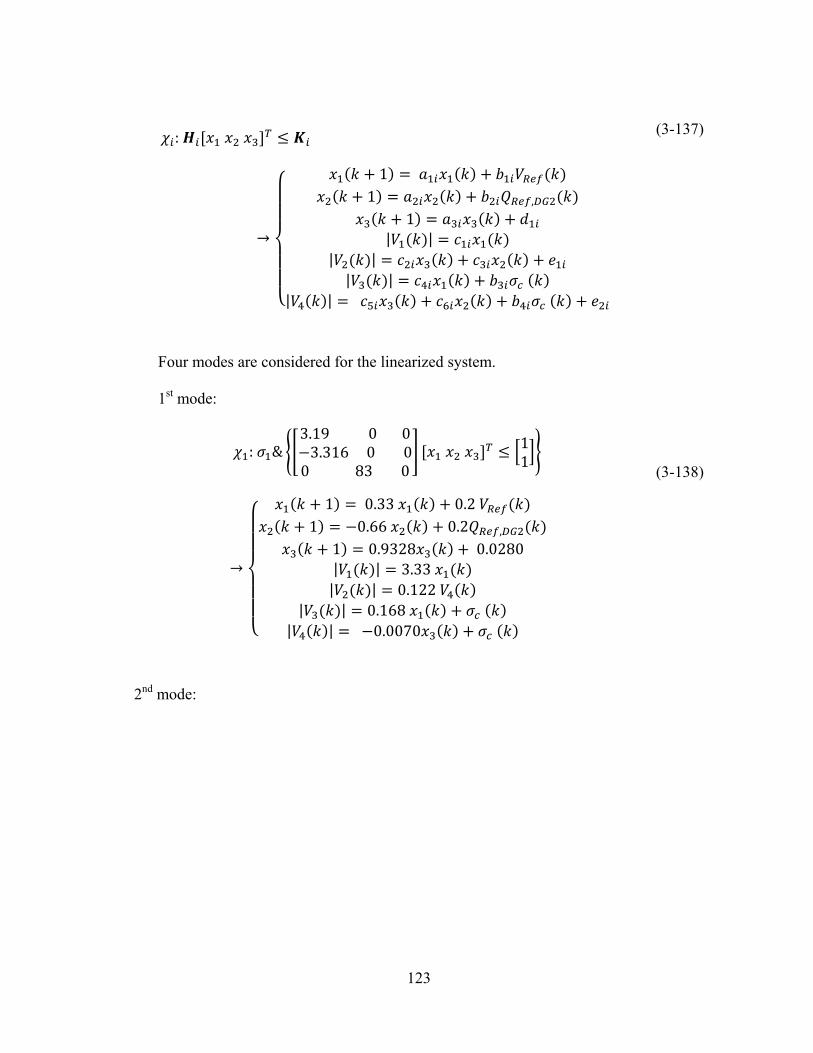
123

:

→

1 1 ,

1| |

| || |

| |

(3-137)

Four modes are considered for the linearized system.

1st mode:

: &3.19 0 03.316 0 00830

11

→

1 0.33 0.21 0.66 0.2 ,

1 0.9328 0.0280| | 3.33| | 0.122

| | 0.168 | | 0.0070

(3-138)

2nd mode:

124

: ~ &3.19 0 03.316 0 00830

111

→

1 0.33 0.21 0.66 0.2 ,

1 0.9328 0.0224| | 3.33| | 0.122

| | 0.168 | | 0.0078

(3-139)

3rd mode:

: &3.19 0 03.316 0 00830

111

→

1 0.33 0.21 0.66 0.2 ,

1 0.9328 0.0280| | 3.33| | 0.093

| | 0.294 | | 0.007

(3-140)

4th mode:

125

χ :~σ &3.19 0 03.316 0 00830

111

→

1 0.33 0.21 0.66 0.2 ,

1 0.9328 0.0224| | 3.33| | 0.093

| | 0.294 | | 0.0079

(3-141)

where σ is an auxillary state switch which represents the system operating with load

profile 1 where only load one is connected to the system and ~σ represents the system

operating in load profile 2 where load 1 and load 2 are both connected to the system.

Further, Auxiliary binary switches through are assigned to hyperplanes

through respectively. This assignment of the auxiliary variables can be shown as

follows.

1 →

1 →

1 →

1 →

(3-142)

We can start by the following change of variables.

1 ∑ , (3-143)

where the state vector is presented as follows.

126

|V k | |V k | |V k | |V k | (3-144)

Further, the control input vector which is consisted of the continuous vector and the

discrete vector is presented as follows.

, (3-145)

The continuous control vector is as follows.

, (3-146)

The discrete control vector is as follows.

(3-147)


vectors as follows.

≜ Max ,.., Max

≜ min ,.., Max (3-148)


equivalent to the following set of equations. In this case, the supremum of the state

variables is 1 and the infimum is -1 as follows.

≜ 1 1 1 1 j=1,..,4

≜ 1 1 1 1 j=1,..,4 (3-149)

127

The vector of auxiliary variables can be defined as follows.

(3-150)

The vector of auxiliary mode selectors, , can be written as follows.

(3-151)

Further, the MLD form could be presented as follows.

1

1

(3-152)

Thus, by enumerating i=1,…,4, the MLD model of the system is presented in the matrix

form as follows.

128

––––

(3-153)

The following conditions also hold for the auxiliary mode selectors.

1 → 0 , 1 → 0 , 1 → 0

1 → 0 , 1 → 0 , 1 → 0

1 → 0 , 1 → 0 , 1 → 0

1 → 0 , 1 → 0 , 1 → 0

(3-154)

Equations (3-135) can be transformed to the following inequality form.

1 0, 1 0, 1 0

1 0, 1 0, 1 0

1 0, 1 0, 1 0

1 0, 1 0, 1 0

(3-155)

129

The objective function for this system is chosen as follows.

, , ‖ | ‖ , …

… ‖ ∆ ‖ , ‖ ∆ ‖ ,

(3-156)

As mentioned in the earlier section u(k)= and V is the nominal voltage

of bus 4.

In this problem, only voltage of bus 4 was included in the objective function because

bus 4 was the main that caused voltage changes in the system, i.e., bus 4 was the only

bus that had uncontrollable changes in the load and generation. In other words, bus 4

experienced load changes based on customer demand and reactive power generation of

the wind generators changes due to the weather condition.

Six case studies were studied for this system as follows.

3.2.5.3.1 Case-study 1 – one wind generator

In this case study one wind turbine with generation capacity of 1 KVA was

connected to bus 4. The synchronous generator in this case study had the capacity of 5.5

KVA. An abrupt load change occurred at t= 6s, where load 2 was connected to the

system. This change was a relatively large change comparing to the inertia of the

synchronous generator. An active load scheme was designed to control the frequency

and supply the active power to the load in timely manner. The active controller is not the

focus of this dissertation. In addition, wind speed changed from 15 m/s to 5 m/s at t=10s

and changed back to normal speed of 15m/s at t=18s. This change in the wind speed

130

resulted in a reduction in reactive power capacity of the wind generator, which means

that other reactive sources in the system should be used to compensate the voltage drop.

The dynamic reactive controller was designed using the MPC discussed in earlier

sections for the objective function (3-156) and the MLD form presented in (3-153).

Figure 3-26 shows the voltage profile of the system and Figure 3-27 shows the control

inputs.

Figure 3-26 Bus voltages of the system for 1 wind generator case

5 10 15 20 250.5

1

Time(s)

V1(

p.u.

)

5 10 15 20 250.5

1

Time(s)

V2(

p.u.

)

5 10 15 20 250.5

1

Time(s)

V3(

p.u.

)

5 10 15 20 250.5

1

Time(s)

V4(

p.u.

)

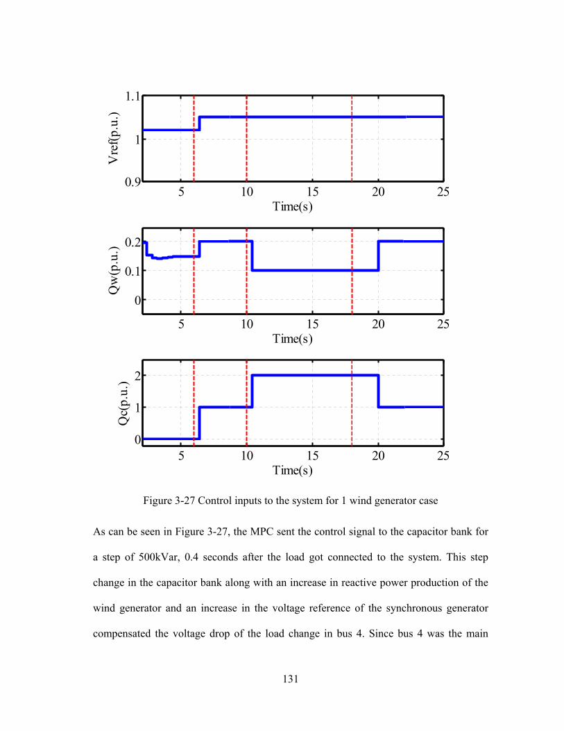
131

Figure 3-27 Control inputs to the system for 1 wind generator case

As can be seen in Figure 3-27, the MPC sent the control signal to the capacitor bank for

a step of 500kVar, 0.4 seconds after the load got connected to the system. This step

change in the capacitor bank along with an increase in reactive power production of the

wind generator and an increase in the voltage reference of the synchronous generator

compensated the voltage drop of the load change in bus 4. Since bus 4 was the main

5 10 15 20 250.9

1

1.1

Time(s)

Vre

f(p.

u.)

5 10 15 20 25

0

0.1

0.2

Time(s)

Qw

(p.u

.)

5 10 15 20 250

1

2

Time(s)

Qc(

p.u.

)

132

reactive consumer in the studied system, compensation of the reactive power in bus 4

consequently resulted in a smooth voltage profile in the whole system.

At t=10s, the wind speed changed to 5m/s which resulted in a drop in reactive power

capacity of the wind generator, therefore, the MPC controller connected the second

capacitor bank to the system to compensate for the reactive power production at bus 4.

When the wind speed changed back to the normal speed, the wind generator took a few

seconds to get back to normal production capacity. When the wind generator got back to

the normal reactive capacity, the MPC controller disconnected one capacitor bank from

the system and used the reactive power production capacity of the wind generator to

compensate for reactive power need in the system.

3.2.5.3.2 Case-study 2 – two wind generators

In this case study two wind turbines with generation capacity of 1 KVA each, were


KVA. The load change and wind change profile was similar to case study 1. Figure 3-28

shows the voltage profile of the system and Figure 3-29 shows the control inputs to the

system for this case study.

133


5 10 15 20 250.5

1

Time(s)

V1(

p.u.

)

5 10 15 20 250.5

1

Time(s)

V2(

p.u.

)

5 10 15 20 250.5

1

Time(s)

V3(

p.u.

)

5 10 15 20 250.5

1

Time(s)

V4(

p.u.

)

134


Although in this case the reactive production was significantly smaller than case study 1

because the percentage of penetration of wind was higher in the system, the MPC

reactive controller was still capable of keeping the bus voltages within limits by

adjusting the control inputs.

5 10 15 20 250.9

1

1.1

Time(s)

Vre

f(p.

u.)

5 10 15 20 25

0

0.1

0.2

Time(s)

Qw

(p.u

.)

5 10 15 20 250

1

2

Time(s)

Qc(

p.u.

)

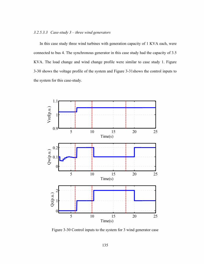
135

3.2.5.3.3 Case-study 3 – three wind generators

In this case study three wind turbines with generation capacity of 1 KVA each, were


KVA. The load change and wind change profile were similar to case study 1. Figure

3-30 shows the voltage profile of the system and Figure 3-31shows the control inputs to

the system for this case-study.


5 10 15 20 250.9

1

1.1

Time(s)

Vre

f(p.

u.)

5 10 15 20 25

0

0.1

0.2

Time(s)

Qw

(p.u

.)

5 10 15 20 250

1

2

Time(s)

Qc(

p.u.

)

136


In this case the reactive production was significantly smaller than case-study 1 and

case-study 2 because the percentage of penetration of wind was higher. However, the

MPC reactive controller was still capable of keeping the bus voltages within limits by

adjusting the control inputs.

5 10 15 20 250.5

1

Time(s)

V1(

p.u.

)

5 10 15 20 250.5

1

Time(s)

V2(

p.u.

)

5 10 15 20 250.5

1

Time(s)

V3(

p.u.

)

5 10 15 20 250.5

1

Time(s)

V4(

p.u.

)

137

3.2.5.3.4 Case-study 4 – one wind generator with half load

In this case study one wind turbine with generation capacity of 1 KVA was

connected to bus 4 and the synchronous generator connected to bus 1 had the capacity of

5.5 KVA. In this case study only load 1 was connected to the system all through the 25

seconds of operation. The wind speed changed from 15 m/s to 5 m/s at t=6s and returned

back to normal speed of 15 m/s at t=18s. The MPC controller tried to eliminate the effect

of reduction of the reactive power capacity of the wind generator.

In this case not only the reactive power controller should keep the voltages above the

lower voltage limit but also should make sure that the control action does not result in

overvoltage in the system. As can be seen in Figure 3-32 and Figure 3-33, the MPC

controller was capable of keeping the bus voltages within voltage limits. In addition, as

can be seen in the results, after the wind speed got back to normal speed, the controller

decided to disconnect the capacitor bank earlier comparing to case-study 1 because the

total consumption of reactive power in the system was smaller in this case than case-

study 1.

138


5 10 15 20 250.9

1

1.1

Time(s)

Vre

f(p.

u.)

5 10 15 20 25

0

0.1

0.2

Time(s)

Qw

(p.u

.)

5 10 15 20 250

1

2

Time(s)

Qc(

p.u.

)

139


3.2.5.3.5 Case-study 5 – two wind generators with half load

In this case study two wind turbines with generation capacity of 1 KVA each, were


KVA. The wind profile in this case-study was similar to case-study 4. Figure 3-34

depicts the control inputs that the MPC controller sent to the system.

5 10 15 20 250.8

11.2

Time(s)

V1(

p.u.

)

5 10 15 20 250.8

11.2

Time(s)

V2(

p.u.

)

5 10 15 20 250.8

11.2

Time(s)

V3(

p.u.

)

5 10 15 20 250.8

11.2

Time(s)

V4(

p.u.

)

140


In this case-study the wind penetration was higher than case-study 4, but as can be

seen in Figure 3-35, the MPC controller was still capable of keeping the bus voltages

within limits.

5 10 15 20 250.9

1

1.1

Time(s)

Vre

f(p.

u.)

5 10 15 20 25

0

0.1

0.2

Time(s)

Qw

(p.u

.)

5 10 15 20 250

1

2

Time(s)

Qc(

p.u.

)

141


3.2.5.3.6 Case-study 6 – Three wind generators with half load

In this case study three wind turbines with generation capacity of 1 KVA each, were

connected to bus 4 and the synchronous generator connected to bus 1 had the capacity of

3.5 KVA.

5 10 15 20 250.8

11.2

Time(s)

V1(

p.u.

)

5 10 15 20 250.8

11.2

Time(s)

V2(

p.u.

)

5 10 15 20 250.8

11.2

Time(s)

V3(

p.u.

)

5 10 15 20 250.8

11.2

Time(s)

V4(

p.u.

)

142

The wind and load profile in this case-study is similar to case-study 4. However the

wind energy penetration is higher in the system. As can be seen in Figure 3-36 and

Figure 3-37, the MPC controller was still capable of keeping the voltages within limits in

this case.


5 10 15 20 250.9

1

1.1

Time(s)

Vre

f(p.

u.)

5 10 15 20 25

0

0.1

0.2

Time(s)

Qw

(p.u

.)

5 10 15 20 250

1

2

Time(s)

Qc(

p.u.

)

143


In this case, the controller connected both of the capacitor banks initially after the

wind speed drop to keep the system stable and then disconnected one of the banks after

the initial disturbance in the system. Similarly, when the wind speed got back to the

normal speed, the controller disconnected both of the capacitor banks initially for

stability purpose and then reconnected one bank to the system.

5 10 15 20 250.8

11.2

Time(s)

V1(

p.u.

)

5 10 15 20 250.8

11.2

Time(s)

V2(

p.u.

)

5 10 15 20 250.8

11.2

Time(s)

V3(

p.u.

)

5 10 15 20 250.8

11.2

Time(s)

V4(

p.u.

)

144

3.3 Model Predictive Control Based Reactive Power Control of Isolated Power

Systems

In this section, the basic concepts and methodologies needed to solve the hybrid

control problem formulated in the section 3.2 will be provided. The section starts with a

brief description of Model Predictive Control (MPC) of power system, which leads to a

mixed integer linear or quadratic programming. Then Mixed Integer Linear

Programming (MILP) and Mixed Integer Quadratic Programming (MIQP) are briefly

discussed.

Model is traditionally referred to differential or difference equations derived from the

physical or circuit dynamics of the studied system. These equations describe the system

as a smooth linear or nonlinear function. Hence, most of the control system theories have

been developed for smooth dynamic systems. However, in most of the cases, the real

system includes logic such as on-off switches and the model of the system is not smooth.

In a power system for example, capacitor banks and tap changers are logic inputs to the

system. Therefore, in most applications including power systems, control of the logic

inputs is performed using heuristic rules derived based on operator’s experience of the

physical system. Although these rules achieve the minimum requirements for some of

the applications, they are not efficient all the times and can get troublesome especially

when the system goes through fast mode changes. Therefore, the relatively new concept

of hybrid systems and hybrid control has been introduced in the literature for this class

of systems [79]. Obviously, the hybrid model of the system is needed for model

145

predictive control. In the next section, some typical methods to model a hybrid system

will be discussed.

3.3.1 Model Predictive Control of Hybrid Systems Described in the MLD Form

MPC can easily solve problems with multiple inputs and outputs and state, input and

output constraint. In addition, most of the hybrid models including MLD and PWA can

be used as prediction models for MPC. This is an interesting feature, which makes MPC

a good candidate for hybrid control problems. More details about the MPC formulation

using MLD models can be found in [79].

MPC works based on a receding horizon policy which means a sequence of future

control actions is chosen based on the prediction of the future behavior of the system and

these control actions are applied to the system until future measurements are available.

When new measurements are available, a new control sequence is calculated over the

shifted horizon and replaces the previous one. This means that the receding horizon

combines the constrained optimal control, which is an open loop procedure with a

receding horizon policy, which provides the feedback to the controller and closes the

control loop. More details about MPC could be found in [113],[114],[115]. The flow

chart of MPC controller is depicted in Figure 3-38.

146

Figure 3-38 Flowchart of the MPC controller

The control sequence is calculated using an optimization which is a Mixed Integer

Quadratic Programming (MIQP) or Mixed Integer Linear Programming (MILP) due to

presence of integer variables in the system. The problem is solved over a finite or

infinite horizon of time using the current state of the plant as initial state. Solving the

problem over infinite horizon achieves best overall controller performance, however, in

majority of the cases a finite horizon is chosen to limit the calculation time. In this

work, a branch and bound algorithm is used to solve the MIQP problem. The branch and

bound algorithm is presented to the extent needed for this dissertation. More details and

full explanation about branch and bound can be found in [116].

147

The optimization problems stemming from MLD systems exhibit some predictable

structural properties. For example, some blocks of constraints are repeated over the

optimization vector due to the evolution of the studied system over the optimization time

horizon. Thus, an efficient B&B algorithm can be designed tailored to the problem

structure to reduce the amount of computation. The number of relaxed QPs (Quadratic

Programs) that have to be solved during B&B gives a measure of complexity of a

solution method for an MIQP. Although this number only gives a rough measure of

complexity since it does not take complexity of the single QPs into account, it often

reflects the time required to find a solution.

The main idea of branch and bound method lies in the fact that QP sub-problems are

relatively easy to solve. In other words, the key concepts in branch and bound are:

Separation of the original MIQP problem into QP sub-problems

Relaxation of the integrality constraints (3-24), meaning that the integer variables

are allowed to span the interval [0, 1].

The optimal solutions to the sub-problems represent lower bounds of the optimal

value of the original MIQP problem [85]. A graphical representation of relaxation and

separation concepts in B&B algorithms for an MIQP with three integers is shown in

Figure 3-39.

148

Figure 3-39 The binary tree for a MIQP with 3 integer variables. Each node is marked with the corresponding vector [116]

A binary tree consists of nodes and branches and one node of the tree is chosen as

the root. Each node except the root has a unique father, which is the predecessor node

towards the root. Each node including the root can have subsequent nodes called

children and a node without children is called a leave. A tree, where each node except

the leaves has exactly k children is called a k-ary tree. The depth of a node is the number

its predecessors towards the root. The q-th level of a tree is the set of all nodes with

depth q. The length of a tree is the maximum depth over all its nodes.

A full k-ary tree of length N is a k-ary tree with leaves, each at depth N. The tree

obtained from a node by deleting the branch to its father and taking as root of a new

tree is the subtree of node .

An MIQP problem can be represented as a tree. Let ∈ 0,1 be a vector having

the same dimension as the vector of binary variables xd, and let the symbol * mean that

the corresponding entry of is relaxed and spans the interval [0, 1]. The original MIQP

149

of (3-23) where all integrality constraints are relaxed is associated to the interval [0, 1]

with the following.

∗ ∗ … ∗ (3-157)

The vector is assigned to the root of a k-ary tree. The separation of the original

MIQP or any sub-problem into relaxed QPs is done by setting selected integer variables

to 0 or 1. The resulting new QP problems are assigned to the children of the node.

Separating the root [* * … *] to two new sub-problems results in the following.

= [* , 0 , * , …, *]

= [* , 1 , * , … , *] (3-158)

Figure 3-40 shows the separation of the root on the second variable.

Figure 3-40 Separation of the roots on the second variable [116]

Each child is represented by a vector , ∈ ∗ ,0,1 and if the i-th component 0

(or 1), then the QP corresponding to that node is solved by setting the i-th integer

variable to 0 (or 1). If ∗, then the i-th integer variable of is regarded as free within

[0, 1] in the corresponding QP.

150

The branch and bound algorithm to solve MIQP can be summarized as follows.

Algorithm 1- Branch and Bound [117]:

1. Initialize a list of sub-problems for the original MIQP problem. Set

fopt = +∞ and xopt = [∞, . . . ,∞]

2. If the list of sub-problems is empty, terminate the algorithm and send fopt and xopt

to output. If fopt = +∞, send an error message that the MIQP is infeasible.

3. Select one sub-problem in the list of sub-problems to become the current problem

and remove it from the list of sub-problems.

4. Relax the current problem, solve it, and denote its solution as fR and its optimizer

as xR. (Relaxation)

5. If the current problem is infeasible go to step 2.

Else if , go to step 2

Else if xR satisfies the integer constraints and , then update the current

best solution by setting fopt = fR and xopt = xR and go to step 2. (fathoming)

6. Generate two new sub-problems from the current problem, add them to the list of

sub-problems, and go to step 2. (Separation)

The performance of a B&B algorithm depends largely on steps 6 and 3. Separation in

step 6 is performed by setting one binary variable to its two possible values. The chosen

binary variable is called branching variable and its selection method defines the

branching rule. The strategy of selecting the next current node in step 3 is called tree

exploring strategy. A good B&B algorithm quickly fathoms large subtrees and avoids

151

formation of numerous sub-problems. The most common choices for the branching rule

and the tree exploring strategy are presented in [117].

In this work, the outside first tree exploring strategy is used to solve the MIQP

problem. The outside first strategy is tailored for optimal control problems using MLD

systems where the values of binary variables occasionally change over the time

horizon, N. The integer optimization vector in (3-24) contains samples of taken

at different time instants.

, 1 , … , 1 (3-159)

Typically, the binary variables are associated with inequality conditions on

continuous states x(k) such as the following.

0 ↔ (3-160)

The continuous states, , usually have to satisfy dynamic equations. Therefore,

their inertia prevents frequent switches of the binary indicator variable . This

observation can be incorporated to make the B&B more efficient. In other words, the

B&B algorithm should try to solve the QPs where the binary switch does not change

prior to the other cases. However, a limited number of switchings should not be imposed

over the prediction horizon since, although unlikely, an arbitrary number of switches

might indeed occur. Therefore, the concept of guaranteed switches is introduced here to

solve the problem.

152

3.3.1.1 Guaranteed switches definition

Given a subproblem given by , let I be the ordered m-tuple collecting the indices i

for which ∗,

≜ , … , such that ∗ ∀ and ⋯

The number of guaranteed switches, D, is defined as the number of indices in I

such that [116].

Example:

Assume 0,0,∗ ,1,∗,∗ ,1,0,0,∗ . With the introduced notation, I = [1, 2, 4, 7, 8, 9],

and D = 2. The outside first tree exploring strategy solves a QP in each column of Table

7 before moving on to the next column.

Table 7 Classification of sub-problems according to guaranteed switches in the binary variables for nd = 3 [116]

Column -1, Original problem

Column 0, no guaranteed switches

Column 1, 1 guaranteed

switch

Column 2, 2 guaranteed switches

[* * *] [0 0 0] [0 0 *] [0 * *] [1 1 1] [1 1 *] [1 * *]

[0 0 1] [0 1 1] [1 1 0] [1 0 0] [0 1 *] [1 0 *]

[0 1 0] [1 0 1]

The order of the QPs in each column is arbitrary. Figure 3-41 shows the order that

outside first strategy uses for exploration of the 3 binary tree. As can be seen in Figure

3-41 and Table 7, the MIQP tree is explored from the outside to the inside.

153

Figure 3-41 Order of solving problems in the outside first strategy, assuming the “first free variable" branching rule [116]

Algorithm 2- Branch and Bound with outside first tree exploring strategy [116]

1. Initialize a list of sub-problems from the original MIQP problem. Set

∞ and ∞, … ,∞

2. If the list of sub-problems is empty, terminate the algorithm and send fopt and xopt

to output. If ∞, the MIQP problem is infeasible.

3. Determine as the minimum number of guaranteed switches among the

problems in the list of sub-problems. Select one problem with guaranteed

switches to become the current problem and remove it from the list of sub-

problems.

4. Relax the current problem, solve it, and denote its solution as fR and its optimizer

as xR.

5. If the current problem is infeasible go to step 2.

Else if go to step 2.

154

Else if xR satisfies the integer constraints and update the current best

solution by setting and .

6. Generate two new sub-problems from the current problem, determine their

guaranteed switches, add them to the list of sub-problems, and go to step 2.

The hard restrictions on computation time due to time-step severely limit the chances

to find a global minimizer to (3-23),(3-24), especially for large power system analysis

problems with many binary variables. Therefore, the MIQP optimization method should

aim at providing sufficient suboptimal solutions. Thus, the method changes the problem

to choosing and solving the problems in the MIQP tree that are most likely to yield to a

sub-optimal point close to the global minimum. Adding a maximum number of

guaranteed switches, kmax, to the outside first tree exploration strategy allows for

selecting and solving the QPs that are most promising in giving good suboptimal

solutions. Bemporad and Morari [79] proved that for MPC problems using MLD

stability is not altered by local minima, even though MPC controller’s rate of

convergence deteriorates.

The block diagram of the proposed model predictive controller based on MLD model

of the MicroGrid is presented in Figure 3-42.

155

Figure 3-42 Block diagram of MPC for the MicroGrid

Summarizing the formulation of this section, the volt/Var optimization problem for

the unbalanced system using the MLD model can be described as follows.

, , |,

∈

|,

|,

‖ ∆ ‖ ,

‖ ∆ ‖ ,

Subj. to

1| | | || || | |

| | 1, … . ,

1, … ,| | 1, … ,

(3-161)

3.4 Performance Analysis of the MPC Controller

As mentioned earlier the system presented in the MLD form is equivalent of PWA

systems and the proof of this can be found in the appendix of [118]. Thus the

156

performance of MPC controlling a system presented in PWA platform which is easier to

present for the general case is presented here. The PWA system is described in the

following general form.

1

(3-162)

where ∈ is the control input to the system and ∈ is the state of the

system. A Lyapanov function with the following general structure is used to prove the

stability of the MPC controller.

(3-163)

where xc is the equilibrium point of the system and satisfies the following conditions.

∶ → ∀ ∈

∀ ∈ → ∈ | | ∞

∀ ∈ → ∈ | | ∞

(3-164)

Possible choices of matrices to guarantee the requirements on the eigenvalues

are

Continuous functions on if is bounded

Constant matrices if is unbounded

It should be mentioned that as shown in [119], the can be discontinuous

around the cell boundaries as long as the number of cells is finite. This is especially

157

helpful when dealing with piecewise systems. The following theorem presents the

requirements for the system to be stable.

Theorem: Assume that the cardinality of the set is finite. Let X0 be a set of initial

states, the equilibrium xc = 0 of the PWA system presented in (3-162) is exponentially

stable on X0 if there exists a function as in (3-163) which results in a negative

forward difference as follows.

∆ 1, 1 1 1

0 (3-165)

where i is the index for the condition ∈ .

This theorem basically means that if a lyapanov energy function can be found that is

dissipative over the time horizon of the controller, then the system is exponentially

stable.

Following [119] and assuming that the eigenvalues of the system are bounded for

each of matrixes and assuming that the set is cardinal there exist constants

, 0 such that

, ∀ ∈ (3-166)

Further, there exist an arbitrarily small such that,

1

(3-167)

158

Since the constant can be chosen arbitrarily small, can be chosen such that

0 1 1. Thus,

∀ ∈ → 1 0 (3-168)

Which directly results in the following.

∀ ∈ → ‖ ‖ 1 ‖ 0 ‖ (3-169)

Equation (3-169) limits the norm of evolution of system trajectory based on the norm

of the starting point.

The second part of our performance analysis of MPC deals with disturbance

attenuation of the platform. To begin with, the so called PWQ stability should be

defined. The following class of lyapanov functions can be used to prove the stability of

the continuous-time PWA systems without logic states [120].

∀ ∈ → (3-170)

Using lyapanov functions of the class (3-170) results in the so-called Piecewise

Quadratic (PWQ) stability. This result can be easily extended to systems with logic

states.

Given a real number 0, the exogenous signal is attenuated by if starting

form a state x0 satisfying C(x0) = 0 for each integer 0 and for ever ∈

0, , 0 it holds

159

‖ ‖ ‖ ‖ (3-171)

Following [118], some preliminary facts on the norm of a PWA system for

which the origin is PWQ stable can be established.

Lemma: Assume that the given system is PWQ stable and set C(x0) = 0. Then, the

constraint is satisfied ∀ where

(3-172)

where,

: Sup ∈ , , : Sup ∈ ‖ ‖

:/

, :

: Sup ∈ , , : Sup ∈ , : Sup ∈ ‖ ‖

(3-173)

The proof of this lemma could be found in [118].

Lemma: Consider an initial state x(0) such that C(x(0))=0. If there exists a function

∀ ∈ satisfying the dissipative inequality (3-165), then the

performance condition (3-171) is satisfied and the PWA system is exponentially

stable.

The proof of this lemma which gives a measure for performance control of PWA

systems could be found in [118].

160

3.5 Summary

This section discussed the problem formulation of dynamic reactive power control of

the isolated power system. First, a simplified model of the system for reactive control

was presented. Then, the model was linearzied in a piecewise linear form and the

resulting linear model was discretized. The piecewise linear model was unified in the

MLD form and the MLD model was used as a prediction model in reactive control.

161

4 MODEL PREDICTIVE BASED REACTIVE POWER CONTROL OF

SHIPBOARD POWER SYSTEMS

4.1 Introduction

As discussed earlier, the AC/DC shipboard power system is consisted of AC

generators and DC distribution zones. The DC zones add to system redundancy and

reliability. The general Volt/Var control for an SPS may take a long time to converge. In

order to shorten convergence time, the general voltage control problem should be

divided into smaller scale sub-problems. It is commonly known that the only active

power can be transmitted over DC links. Thus, the reactive power control can be

decoupled into smaller scale problems by cutting the system at the DC links. Decoupling

the Volt/Var control into smaller problems is beneficial since the

The high voltage AC system includes the synchronous generators, propulsion

motors, and potentially high power pulsed AC loads. The high voltage AC system treats

the DC zones as AC loads connected to the AC bus. The AC system also may include

reactive power compensators placed close to loads at design stage. The voltage control

scheme in this work, solves the voltage control problem of the AC system dynamically

and sends reference voltage of generators and reactive power setpoints of compensators

to these components. The optimization problem minimizes the voltage deviation of

specific buses in the system, which are more vulnerable to voltage drop by setting the

optimal control inputs.

The voltage control of the each DC zone is solved separately and locally in this work.

Thus, each distribution zone is able to keep the voltage autonomously. The Zone is

162

composed of DC/DC converters, Inverters, DC and AC loads. The converters and

inverters are the main components that can be used for voltage control inside the zones.

Obviously, the rectifier can also be used to control the voltage level of the main DC

buses of the system. The control scheme is local and the components are coordinated to

keep the voltages of the buses within limits.

4.2 Implementation and Simulation Results

The sample SPS used in this paper for the case-studies is depicted in Figure 4-1. The

system is composed of two synchronous generators, two zones and one propulsion

motor. The objective function for the studied SPS is as follows.

, , |∈ , , ,

‖ ∆ ‖ (4-1)

The control inputs to the system are reference voltages of generators ( , )

and the reactive power setpoint of the dynamic compensator ( ). Thus, the control input

vector is as follows.

, , (4-2)

163

Figure 4-1 Schematic diagram of a notional all electric shipboard power system

164

The system has one master generator which is the main generator (MTG) and one

distributed synchronous generator which is the auxiliary generator (ATG) in this case.

The propulsion motor, two zones and the pulsed load are modeled as dynamic loads.

Since the system had one master generator, one distributed generator, and three dynamic

loads, the number of the states of the system was five.

Figure 4-2 shows the high level schematic diagram of the notional shipboard power

system.

Figure 4-2 High level schematic diagram of a notional all electric shipboard power system

For the master DG, the simplified state space equations are as follows.

1

1

(4-3)

For the other DG in the system, the simplified state space equations are as follows.

165

1

,,

,1

,

(4-4)

Similarly, following (3-65) for the dynamic loads in the system, the linearized state

space equations are as follows.

1

, ,,

5,6,7, 4,7,8

, ,1

,

,

(4-5)

where ’s are the voltage of the buses with the loads connected to them. Following the

linearization technique discussed in [111], piecewise linear equations of the system are

derived as follows.

11

⋮1

(4-6)

The bus voltages could be described in compact form as follows.

1⋮

1

(4-7)

where is the vector of the voltages that are used in the optimization formulation.

Increasing the number of sets makes the prediction of voltage more accurate; however,

the optimization algorithm takes more time to converge to the global minimum.

166

The input weight matrix is defined as 0.1, 0.1,0.01 which is designed to

penalize the reactive power compensator less than the generators since providing

reactive power by the reactive compensators is less costly.

The voltage, current and reactive power constraints of the SPS are given by

following equations.

| | 3,4

| | 1, … , 4

(4-8)




The nonlinear SPS model with all details is implemented in SIMULINK and is

considered as the actual power system. The measurements are taken from this power

system and send as feedback to the model predictive controller. The MPC uses the MLD

model achieved from HYSDEL compiler as the prediction model and performs the

optimization over the horizon 10 seconds using the feedback of the system as the initial

state. Solving the optimization problem results in the optimal control sequence, which is

sent to the generators and the compensator of the SPS. The parameters of the generators

are presented in Table 8.

167

Table 8 Generator parameters of the notional SPS Generator Parameters Exciter Parameters

MTG ATG MTG/ATG

VgI-I 13.8kV 13.8kV Tc 0s

Pg 36 MW 4 MW Tb 0s pfg 0.8 0.8 Ka 400pu F 60 Hz 60 Hz Te 0.02s Ra 0.010Ω 0.199Ω Va,max 14.5pu Xp 0.17 0.18 Va,min 14.5pu (neg) Xd 1.55 1.25 Vr, max 6.03pu Xd' 0.22 0.24 Vr,min 5.43pu (neg) Xd'' 0.14 0.17 kf 0.03pu Tdo' 8.95s 4.11s Tf 1s Tdo'' 0.036s 0.023s Te 0.8s Xq 0.76 0.62 Ke 1pu Xq' N.A N.A kc 0.2pu Xq'' 0.20 0.26 kd 0.38pu Tqo' N.A N.A SE(VE1) 0.1pu Tqo'' 0.12 s 0.061s

H 1.49s 1.06s

The load and line parameters are summarized in Table 9 an the line lengths are

presented in Table 10.

Table 9 Load and line parameters of the notional SPS Load parameters Value Load parameters Value

36 MW bt 2

9 MVar T 5s

, 4e6 MW T ,T 3s

, 1.8e6 MVar T 3s bs 1

168

Table 10 AC line length of the notional SPS AC Line Line length Line 1 50m Line 2 20m Line 3 20m Line 4 30m

Three voltage control case studies have been studied for the system.

4.2.1 Case-study 1- No Dynamic Compensator

In this case study, the SPS did not include a dynamic reactive compensator. A pulsed

load was connected to bus 4 at t=2s for a duration of 2 seconds. It was assumed that the

MPC knows the exact time of operation of the pulsed load. As can be seen in Figure 4-3,

the MPC controller tried to compensate for the voltage drop by simultaneously boosting

the excitation of the MTG and ATG generators. However, Figure 4-4 shows that the

voltages of bus 3 and bus 4 dropped below the minimum acceptable level. In addition,

overly boosting of the excitation of the synchronous generators resulted in a high voltage

ripple on all the AC buses in the system and overcurrent of generator. This phenomenon

deteriorates the electrical circuits of the generator. However, the controller could not

avoid this condition since it needed to keep the system stable.

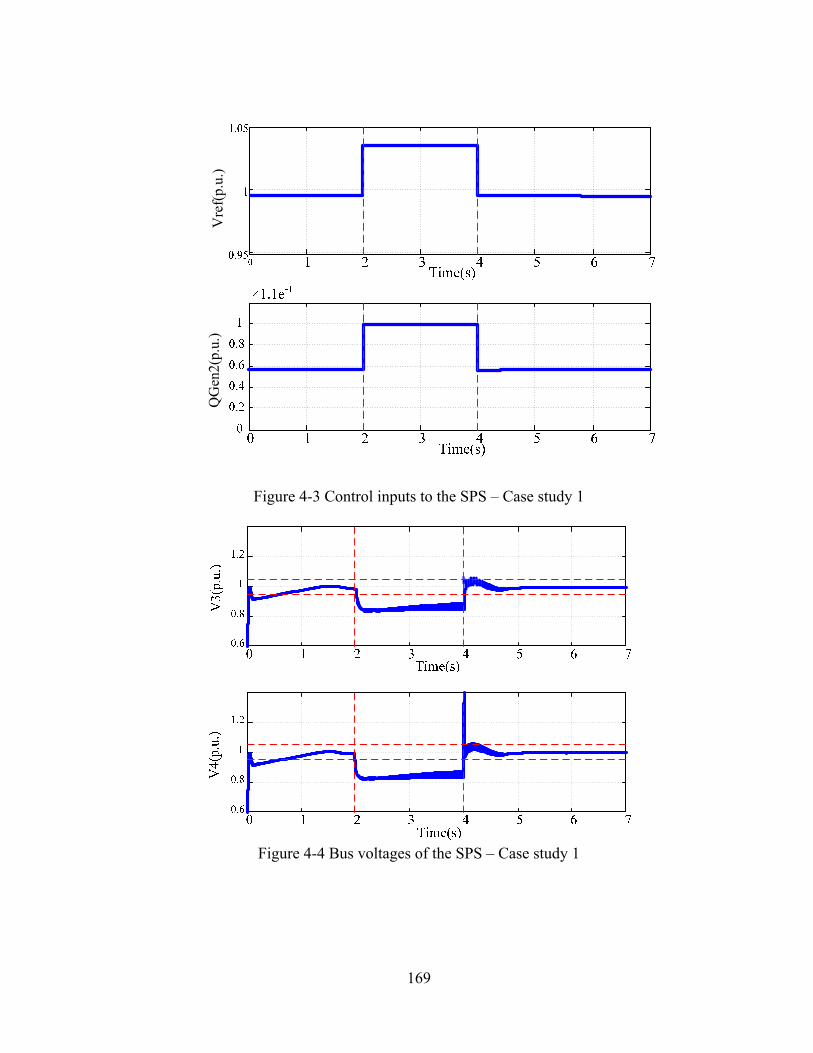
169

Vre

f(p.

u.)

QG

en2(

p.u.

)

Figure 4-3 Control inputs to the SPS – Case study 1

Figure 4-4 Bus voltages of the SPS – Case study 1

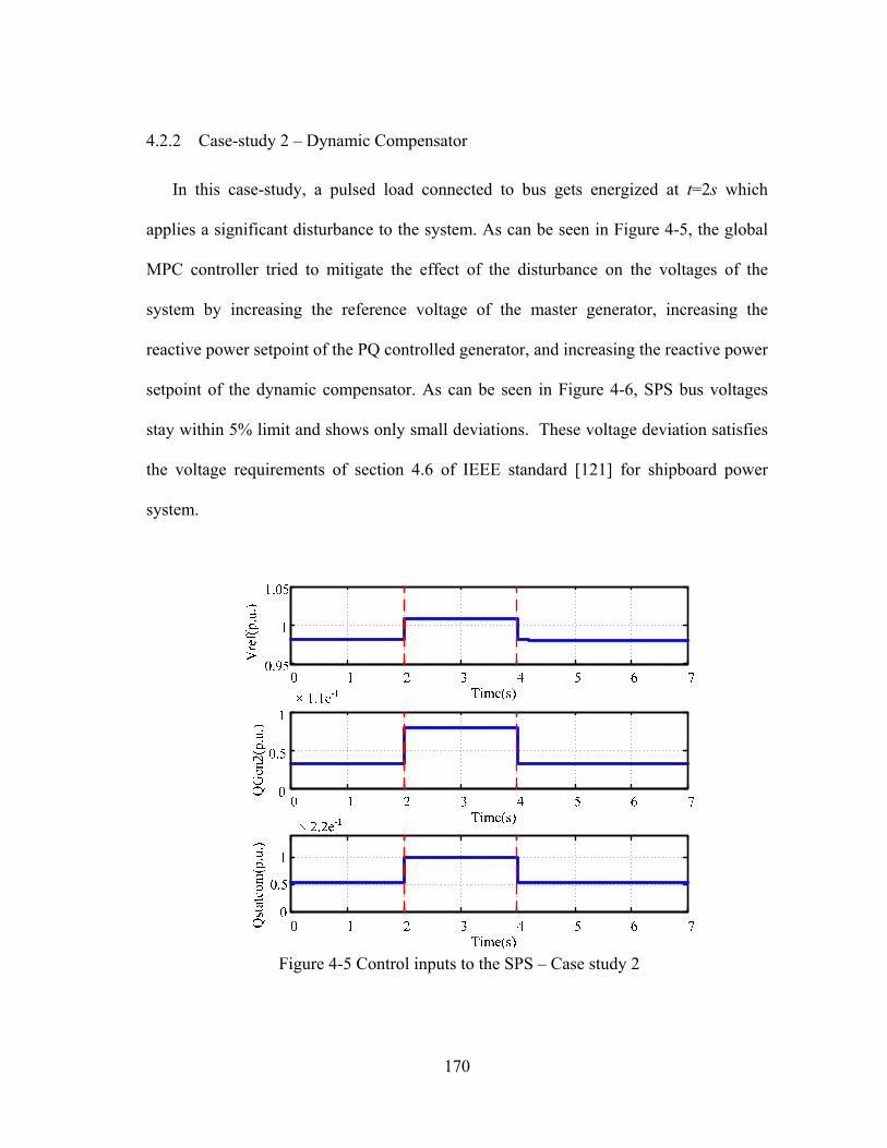
170

4.2.2 Case-study 2 – Dynamic Compensator

In this case-study, a pulsed load connected to bus gets energized at t=2s which

applies a significant disturbance to the system. As can be seen in Figure 4-5, the global

MPC controller tried to mitigate the effect of the disturbance on the voltages of the

system by increasing the reference voltage of the master generator, increasing the

reactive power setpoint of the PQ controlled generator, and increasing the reactive power

setpoint of the dynamic compensator. As can be seen in Figure 4-6, SPS bus voltages

stay within 5% limit and shows only small deviations. These voltage deviation satisfies

the voltage requirements of section 4.6 of IEEE standard [121] for shipboard power

system.


171


4.2.3 Case-study 3- Propulsion motor speed change

In this case-study, the speed of the propulsion motor changes from 2/3 of the

nominal speed to the full nominal speed at t=9s. The inrush current that the induction

motor is drawing from the system causes a disturbance in the system. This disturbance

can be modeled as a pulse of reactive power drawn from the system, which causes

voltage drop. The global MPC controller tries to mitigate the effect of the disturbance

on the voltages of the system. The controller reacts to the voltage drop in 0.2 seconds.

The bus voltages are depicted in Figure 4-7.

0 1 2 3 4 5 6 70.6

0.8

1

1.2

g

Time(s)

V3(

p.u.

)

0 1 2 3 4 5 6 70.6

0.8

1

1.2

1.4

Time(s)

V4(

p.u.

)

172


The control inputs generated by the MPC controller are shown in Figure 4-8. The

controller increased the voltage reference of the master generator, increased the reactive

power injection by the PQ generator, and increased the reactive injection by the D-

STATCOM to achieve the reactive power control goals.

7 8 9 10 11 12 13 14 150.6

0.8

1

1.2

Time(s)

V3(

p.u.

)

7 8 9 10 11 12 13 14 150.6

0.8

1

1.2

Time(s)

V4(

p.u.

)

173


4.3 Local Control of DC Distribution Zones

In this section, the structure of the DC distribution zone is discussed first. Then local

voltage control scheme of the DC zone is discussed briefly. As mentioned before,

voltage control of each DC zone is a sub-problem to the global voltage control problem

and is solved locally.

The DC distribution zones are composed on DC/DC converters, Inverters, AC and

DC loads. The loads can be vital and non-vital depending on the importance of their

functionality. Vital loads typically have two possible paths to get energized. This

174

redundancy helps the system to keep the vital loads energized if one of the paths

experience fault. The general structure of a DC zone is depicted in Figure 4-9. Each zone

has a rectifier which supplies DC power to the zone. The rectifier, converter and the

inverter are coordinated together to keep the voltage of the load at the nominal level.

4.4 Summary

This section discussed reactive power and voltage control of the SPS. The problem

was formulated considering the dynamics of the SPS. MATLAB and CPLEX were used

to implement the method. Finally, some case-studies were presented to show the

effectiveness of the algorithm. Effectiveness of the methods was studied in presence of

pulsed dynamic loads and changes in the propulsion of the ship.

g

sV

dggs iL

dgi

)(td)(sGc

)(sH

refv

ev CHv

D

d

qgi

dgi*dgv

qgv

dggs iL

Figure 4-9 Block diagram of local controller to control the voltage of DC zones

175

5 MODEL PREDICTIVE BASED REACTIVE POWER CONTROL OF

MICROGRIDS

5.1 Introduction

Voltage control is crucial in operation of the MicroGrid and the utility is responsible

to keep the voltage at the receiving end of the distribution line within the acceptable

range. The ANSI C84.1 standard specifies a guideline for the acceptable range by

dividing it into emergency and normal operating ranges. The system may operate in the

emergency range only for a short amount of time. Thus, the normal operating range is

the focus for system operation. The ANSI C84.1 service voltage ranges are shown in

Table 11.

Table 11 ANSI C84.1 voltage range for 120v [122]

Service

Min Max

Range A (Normal) -5% +5%

Range B (Emergency) -8.3% +5.8%

It should be noted that since the distribution system is usually radial, the service

voltage is the main feeder voltage minus the losses on the transformers and lines in

absence of DERs. Thus, the utility usually controls the service voltage by controlling the

feeder voltage and sometimes by switching on load tap changers and switched capacitor

banks. However, when the DERs are present in the system, the operator can also use

176

them to control the voltage especially when the DERs are interfaced to the system using

power electronics. Further, in a system that may have to operate in islanded mode such

as a MicroGrid, controlling the feeder voltage directly through the main grid is no longer

possible. Thus, the DERs, reactive power compensators, and tap changers are the only

voltage control inputs to the system in the islanded mode. A number of publications are

available in the literature that discuss the challenges and benefits of using inverter-based

DERs for voltage support [123],[124].

5.2 Photovoltaic Source

With an annual growth rate of 25-35%, photovoltaic sources are among the fastest

growing energy sources over the past decade. Prior to 1999, the primary market for PV

source was in off-grid applications. However, over 80% of the recent market for the PV

source is for grid-connected applications where the source is connected to a strong grid

or an isolated grid as a distributed generator [125]. As the use of PV sources continues to

expand, research on potential benefits and risks that the PV source introduces on the

stability and operation of the electricity grid grows as well.

The impact of the PV on the voltage of the grid is directly related to its penetration level.

Generally, the PVs can be classified into three categories for voltage control based on

their penetration level in the grid:

1) At a low PV penetration level of 5% or less, the inverters generally do not have a

significant impact on the feeder’s voltage regulation

2) At medium PV penetration levels which is around 10%, inverter voltage support

can help reduce the size of the voltage support capacitors by nearly 40%

177

3) At high PV penetration levels (30% – 50%), PV inverters may be able to entirely

replace voltage support capacitors

At higher penetration levels, inverter-connected PV generation takes over the place

of conventional generation. In order to match the performance of the conventional

generators, inverters have to be able to exchange reactive power with the grid. Certain

changes in control and protection schemes may need to be performed to adapt the PV for

voltage control. Inverter ratings may need to be increased to allow more significant

impact on voltage control and the operation of inverters has to be coordinated to take full

advantage of the available reactive power capabilities of the inverters [126]. The

coordination can be performed using local methods such as the methods presented in

[127],[128] or through a global optimal control scheme that sends the reactive setpoints

to the inverters dynamically.

Solving the global optimization problem gives the setpoint of the reactive power Q

of the units in the MicroGrid. The setpoints are used in control of the DG unit or to

determine the injection by the reactive compensators. The DG units also have their own

droop control which fine tunes the reactive setpoint to keep the voltage within limits.

The droop control is needed for voltage stability and local reliability and to avoid

voltage and reactive power oscillations. It also eliminates the effect of small errors in the

setpoint [61]. The mentioned DG control structure is shown in Figure 5-1.

“sh

pro

agr

it i

inc

inc

wit

nee

cap

am

Th

Currently,

hall not acti

ovide active

reement to m

is not due

corporates th

crease the be

th most of th

ed to be upd

With simp

pable of pro

mount is limi

is concept i

Figu

standards s

vely regulat

power to th

make the PV

to the limit

he reactive

enefits of in

he current an

ated as well

ple modifica

viding react

ted by the r

is illustrated

ure 5-1 Contr

such as IEE

te the voltag

he grid in cu

Vs generate th

tations of th

power cap

nverter-based

nti-islanding

in most case

ations in co

tive power t

ate of the in

d in Figure

178

rol scheme o

EE 1547 and

ge at the PC

urrent imple

he maximum

he inverters

abilities of

d DERs to t

g schemes [1

es.

ntrol schem

to the grid in

nverter and t

5-2 for a un

of a DG unit

d UL1741

CC.” Thus,

ementations.

m possible am

s. A voltag

the PV so

the grid. Un

129]. Thus,

me, most of

n addition to

the amount o

nidirectiona

[61]

state that th

PV system

. However,

mount of act

ge regulation

ources would

nfortunately,

the anti-isla

f the current

o the active

of generated

l inverter w

he PV inver

ms operate on

this is only

tive power a

n scheme th

d significan

this interfe

anding schem

t inverters

power but t

d active pow

where inverte

rter

nly

an

and

hat

ntly

eres

mes

are

the

wer.

er's

179

ratings are represented by a vector with magnitude S, the generated active power by the

PV cells are denoted by Ppv.

The semicircle with radius S shows the inverter’s possible operation range.

Obviously, the feasible reactive range of the inverter is limited by the amount of

generated active power. Reactive power limits are shown by -Qlimit and Qlimit which

shows that the inverter is capable of absorbing and injecting reactive power,

respectively. Thus, theoretically the inverter is able to use its full rated power for

reactive compensation when the generated real power is zero and cannot supply any

reactive power when the full rating is used for generation of active power [126]. One

method to overcome this drawback is to keep some reactive capability by over-sizing the

inverter by 10-20%. The incentives for the DER operator to provide reactive power are

increasing and maybe it becomes equal to the incentive of providing active power [1].

Figure 5-2 Reactive power generation limits by the PV inverter [126]

180

5.3 DFIG Wind Generator

DFIGs have become very common in wind power industry in the past decade. As

explained before DFIGs need smaller converter than their rated power and are able to

operate in variable-speed. Variable speed operation makes it possible to increase annual

power production by 5% [130].

The stator of the DFIG is directly connected to the gird while the rotor is connected

to the gird through a power electronics converter. The DFIG always supplies electric

power to the grid from its stator and exchanges power with the grid from its rotor. The

rotor power usually does not exceed 25% of the total generator power. The converter of

the DFIG needs to be rated to handle rotor power and the excitation of the generator

[131]. Thus, the converter rating is usually around 25% of the rated power of the

generator, which results in lower component cost.

Squirrel cage induction generators were very common in wind industry two decades

ago and they are still present. However, DFIGs and permanent magnet generators are

taking their place due to some major advantages. These advantages include ability of

DFIGs to control reactive power and voltage [132] and the potential to control active and

reactive power independently through control of torque and rotor excitation current

[133].

Although the grid requirements usually require the DFIGs to be reactive neutral, they

can be used for reactive power control in some circumstances. The operating conditions

of the DFIG can be classified into two categories based on the power grid they are

connected to. These categories are as follows [134]:

181

When DFIG is connected to strong power system the voltage is usually set to 1

PU. In this case, the DFIG does not exchange reactive power with the grid.

When DFIG is connected to a weak power system, which suffers from

fluctuating voltages, the DFIG can be used to produce or absorb reactive power

for voltage control.

In the latter case, a PI controller can be added per customers request [135] to produce

the reference signal of reactive power from the voltage error at the generator bus [136].

This type of control scheme controls reactive power locally and helps with grid voltage

support. However, the results are not globally optimal due to the local nature of the

control scheme.

The current grid code requires the wind farm to be reactive neutral and limits the

control of reactive power absorption and generation through the wind farm to 10% of the

maximum power [15]. However, it is beneficial to use reactive power capabilities of the

DFIG generators for voltage compensation in weak power grid such as the MicroGrid. In

MicroGrids for example, the grid side converter may be overdesigned to be able to inject

or absorb 25-30% reactive power to the grid. Overdesigning the converter can be

beneficial to overcome voltage fluctuations during fault condition.

Based on current grid code, the total time from the occurrence of a fault until

establishment of normal voltage may not take more than 10 seconds [15]. Long voltage

drops below 60-80% after a fault usually indicated that the turbine has accelerated too

much that the power system cannot take it back to normal speed. The current control

scheme performs a fast reduction of active power and a fast increase in reactive power to

182

overcome this situation. This scenario shows that overdesigning the converter can be

helpful to post-fault voltage drops since more reactive power could be generated with

less decrease in active power generation. Thus post-fault voltage compensation takes

shorter time.

5.4 Connecting DERs to the Grid

Recent surveys show that the interconnection concerns from the electric utility point

of view include reliability of the existing grid, the safety of electric power system

personnel, and quality control. Thus, universal technical standards that permit

standardized grid interconnection of the DERs while maintaining power system stability

and worker safety is important in the MicroGrid design. The Institute of Electrical and

Electronic Engineers (IEEE) presented a universal interconnection standard in winter of

1999 which is currently called IEEE P1547 standard [137]. The IEEE P1547 standard

presents a uniform design standard for interconnection of DERs of 10 MVA or smaller

with electric power systems. The requirements relevant to performance, operation,

testing, safety, and maintenance of the interconnection are also included in the standard.

Currently, the states of California, Texas, New York, and others have also set forth their

own DER interconnection requirements [138].

The reactive power requirements of the MicroGrid during the islanded mode are

important to consider in the design stage. DERs and compensators should be able to

provide real and reactive requirements of the loads at an acceptable voltage level in the

islanded mode operation of the MicroGrid. The reactive power requirements of the load

during islanded mode operation and the reactive power resources should be studied in

183

the design stage. Particularly, reactive power resources need to be sufficient not only to

provide steady-state reactive power demands, but also to provide dynamic reactive

power demands, such as those related to motor starting within islanded MicroGrid.

There needs to be sufficient reactive power resources available when operating induction

machines or some inverter-based loads. Synchronous generators can typically provide

rated power at 0.8 lagging power factor. Thus, it is important to include other sources of

reactive power (e.g. capacitors) when designing the island system if the load’s reactive

requirements are far greater than the rating. Otherwise, the MicroGrid may not be able to

provide the full-rated real power and that the generator’s operation may be degraded

[137].

In the local control scheme, the reactive power sharing operates under the following

control method. The system reactive load level is provided to all of the generators

operating on the common isolated bus. Then, each generator adjusts its own reactive

power output to match the system-average reactive load. This is a closed-loop control

method that is usually implemented with a proportional, integral, derivative (PID)

algorithm, which results in more even control with less required readjustment to

maintain satisfactory results. Unlike droop control, voltage control of the islanded

system can be maintained by a control algorithm that corrects for low or high system

voltage. The voltage-correction feedback is applied to all of the generators to maintain

the desired system voltage.

Reactive power sharing requires that the system reactive power average be

communicated to all generators. This is commonly achieved using an analog control

184

signal or digital control communication. In this approach, specifics of the equipment,

interfaces, and available communications protocols may present challenges [106].

The protection devices placed at the interconnection of the DER to the power system

measure the effective voltage and the fundamental frequency of the phase-to-phase

voltages and if the measured voltage is in a range given in Table 12, the DER should

stop energizing the area within the clearing time as indicated in the table. Clearing time

is the maximum allowed time between the start of the abnormal condition and the DER

disconnection from the system. For DERs smaller than or equal to 30 kW, the clearing

time and voltage setpoint could be field adjustable or fixed. However, the voltage set

points should be field adjustable for the DERs greater than 30 kW. The voltages shall be

detected at either the PCC or the point of DER connection when any of the following

conditions exist:

a) The aggregate capacity of DER systems connected to a single PCC is less than or

equal to 30 kW,

b) The interconnection equipment is certified to pass a non-islanding test for the

system to which it is to be connected,

c) The aggregate DER capacity is less than 50% of the total Local EPS minimum

annual integrated electrical demand for a 15 minute time period, and export of real or

reactive power by the DER to the area is not permitted [139].

It should be mentioned that the numbers mentioned in Table 12 are subject to change

for isolated power systems. Isolated power systems typically have less strict

requirements on voltage levels than grid connected systems [106]. The requirements for

185

isolated systems may vary from one system to another and are usually defined during

system design.

Table 12 Requested fault clearing time for isolated power systems Voltage range (% of

base voltagea) Clearing time(s)

V<50 0.16

50<V<88 2.00

110<V<120 1.00

V>120 0.16

Placement of the DGs requires extensive studies on the MicroGrid. The weakest bus

searching [140] is a simple method for DG placement. This method tries to maximize the

loadability of a distribution system by placing a single DG at the weakest bus of the

system. However, methods such as weakest bus or the largest load bus may not always

lead to the best location for loss reduction and are not effective for placement of multiple

DGs. Thus, an optimization problem to minimize the total cost and the active power loss

should be solved in most cases. Optimal distributed generation (DG) placement [141] is

usually formulated as a mixed integer nonlinear programming problem aiming at

minimizing the total cost or the total active power loss. The optimal placement problem

has been solved by a variety of optimization and search methods in the literature

including repetitive load flow [142], the weakest bus searching [140], particle swarm

intelligence [143], genetic algorithm [144], and linear programming [145].

186

5.5 Implementation and Simulation Results

As mentioned earlier, direct modeling of hybrid systems in MLD form is usually

time consuming. In this work, HYbrid Systems DEscription Language (HYSDEL) [83]

was used to derive the MLD form of the system. This program has a compiler that

converts the textual description of the system to the MLD form. The MLD model of the

system is then used as the prediction model in the MPC scheme. The MPT toolbox was

used to solve the optimization problem. The MPT toolbox uses a branch and bound

algorithm to solve the multi-parametric programming. Solving the multi-parametric

problem leads to solving LP or QP problem and efficient solvers exist for these

problems. CPLEX 12.2 engine was used to solve the MIQP.

5.5.1 Studies on an 11 bus MicroGrid

One MicroGrid studied in this work is depicted in Figure 5-3. The system was

composed of four Distributed Generators (DGs), 11 buses, and some dynamic and static

loads. The DGs were consisted of one diesel generator, 2 wind generators, and one solar

generator. Two reactive power compensators were also present in the system which will

be discussed more in the case-studies.

187

Figure 5-3 Schematic diagram of the studied MicroGrid

Parameters of the sources are presented in Table 13.

Table 13 Source parameters of the 11 bus MicroGrid

Diesel Quantity Wind & Solar Quantity

VgI-I 575V VgI-I (wind) 575V Pg 1MW Pg (wind) 0.4 MW pfg 0.8 Vs 400 V f 60 Hz Vr 1975 V

Ra 0.199Ω F 60 Hz Xp 0.18 Rs 0.023 (p.u.) Xd 1.25 Ls 0.18 (p.u.) Xd' 0.24 Rr 0.016 (p.u.) Xd'' 0.17 Lr 0.16 (p.u.) Tdo' 4.11s Lm 2.9 (p.u.) Tdo'' 0.023s H 0.685 (p.u.) Xq 0.62 f (wind) 0.01 (p.u.) Xq' N.A Poles 3 Xq'' 0.26 Tqo' N.A VgI-I (solar) 575V

Tqo'' 0.061s Pg (solar) 0.4 MW

H 1.06s f (solar) 60 Hz

188

The objective function for reactive power control of the MicroGrid shown in Figure 5-3

was chosen as follows.

, , |

∈ , , ,

‖ ∆ ‖ ‖ ∆ ‖

(5-1)

Control inputs to the system were the reference voltage of synchronous diesel

generator ( ), reactive power setpoints of the DGs, and the reactive power setpoint of

the dynamic compensator ( , ). Thus, the control input vectors were as follows for

the case where power electronics compensators were placed in the MicroGrid.

, , , , , , 0,0 (5-2)

For the case studies where capacitor banks were placed in the system the control input

vectors were as follows.

, , , , , (5-3)

Since the system had four distributed generators, and two dynamic loads, the number

of the states of the system was six. For the master DG, the simplified state space

equations were as follows.

1

1

(5-4)

189

For the other DGs in the system, the simplified state space equations were as follows.

1

,,

,1

, , 2,3,4

(5-5)

Similarly, following (3-65) for the dynamic loads in the system, the linearized state

space equations were as follows.

1

, ,,

5,6,7, 4,7,8

, ,1

,

,

(5-6)

where ’s are the voltage of the buses with the loads connected to them. Following the

linearization technique discussed in [111], piecewise linear equations of the system were

derived as follows.

11

⋮1

(5-7)

The bus voltages can be described in compact form as follows.

1⋮

1

(5-8)

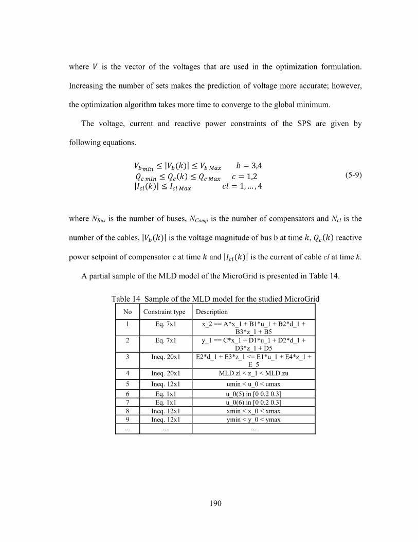
190

where is the vector of the voltages that are used in the optimization formulation.

Increasing the number of sets makes the prediction of voltage more accurate; however,

the optimization algorithm takes more time to converge to the global minimum.

The voltage, current and reactive power constraints of the SPS are given by

following equations.

| | 3,4

1,2 | | 1, … , 4

(5-9)




A partial sample of the MLD model of the MicroGrid is presented in Table 14.

Table 14 Sample of the MLD model for the studied MicroGrid

No Constraint type Description

1 Eq. 7x1 x_2 == A*x_1 + B1*u_1 + B2*d_1 + B3*z_1 + B5

2 Eq. 7x1 y_1 == C*x_1 + D1*u_1 + D2*d_1 + D3*z_1 + D5

3 Ineq. 20x1 E2*d_1 + E3*z_1 <= E1*u_1 + E4*z_1 + E_5

4 Ineq. 20x1 MLD.zl < z_1 < MLD.zu

5 Ineq. 12x1 umin < u_0 < umax

6 Eq. 1x1 u_0(5) in [0 0.2 0.3] 7 Eq. 1x1 u_0(6) in [0 0.2 0.3] 8 Ineq. 12x1 xmin < x_0 < xmax 9 Ineq. 12x1 ymin < y_0 < ymax

… … …

191

The photovoltaic source was controlled using an MPPT algorithm. The controller of

the wind generator was also designed to send the maximum active power to the system

and the reactive power was regulated through an external PID. Details of the MPPT and

local controller are beyond the scope of this dissertation.

The loads are modeled in the prediction model as dynamic loads and the MLD model

of the system was derived with the approach discussed in the paper for a horizon of 12

time steps ahead and each time step is 0.2 seconds. The input weight matrix was defined

as 0.1, 0.01,0.01,0.01 , 15,15 which was designed to penalize the

reactive power compensator less than the generators since providing reactive power by

the reactive compensators is less costly.

The studied MicroGrid with all details was implemented in SIMULINK and was

considered as the actual power system. The measurements were taken from this power

system and sent as feedback to the model predictive controller. The MPC used the MLD

model achieved from HYSDEL compiler as the prediction model and performed the

optimization over the horizon N using the feedback of the system as the initial state.

Solving the optimization problem resulted in the optimal control sequence, which was

sent to the sources and the compensators of the MicroGrid.

The load and line parameters of the studied MicroGrid are summarized in Table 15.

192

Table 15 Load and line parameters of the 11 bus MicroGrid

Symbol Quantity Symbol Quantity

PL0-1 0.1 MW QL-4 0.03 MVar QL0-1 0.2 MVar PL-5 0.1 p.u. PL0-2 0.1 MW QL-5 0 QL0-2 0.1 MVar PL-6 0.02 p.u. PL0-3 0.1 MW QL-6 0.07 p.u. QL0-3 0.1 MVar PL-7 0.1 p.u. bs1-3 1 QL-7 0 bt1-3 2 PL-8 0.10 MW Tq1-3 3sec QL-8 0 MVar PL 10 0.05 MW PL-9 0.2 MW

QL 10 0.2 MVar QL-9 0.1 MVar

PL 11 0.2 MW QL 11 0 MVar

PL-4 0.05 MW

5.5.1.1 Case-study 1

In this case-study, loads 7,10 got connected at t=2s in the sample MicroGrid shown

in Figure 5-3. These loads remained connected until t=3.2s where load 7 was

disconnected but load 10 stayed connected to the system. In this case study, capacitor

banks were considered as reactive power compensators and were connected to bus 6,7.

In this case study, capacitor banks were considered as reactive power compensators and

were connected to bus 6,7. Two capacitor banks rated 150 kVar were connected to bus 6

and two capacitor banks each rated at 100 kVar were connected to bus 7. The time

horizon was selected as 12 and the step time was considered to be 0.2s. The prediction

model was implemented in HYSDEL which transfers the model to MLD form. The

193

MLD was used as prediction model and the optimization was performed using CPLEX

12.2.

The optimization problem led to solving a Mixed Integer Quadratic Programming

(MIQP) problem since norm 2 was used in the objective function. The voltages of the

load buses are shown in Figure 5-4 and the control inputs are depicted in Figure 5-5. As

can be seen in the figure, the dynamic reactive controller responded faster to the change

in the load and results in smoother voltage profile. The active and reactive power

tracking of the wind generator 1 and the PV source are depicted in Figure 5-6 and Figure

5-7 respectively.

Figure 5-4 RMS voltage of bus 5,6,7,8 – MPC (solid line), Local Control (dashed line) in case study 1

194

As can be seen in Figure 5-5, the controller adjusted the reactive power coordination

by decreasing the voltage reference of the master generator, decreasing the reactive

power setpoint of wind generators and the solar generator, and adding two capacitor

banks at the connection point of capacitor 2. After one the loads gets energized, the

controller responds by disconnecting one capacitor at the connection point of capacitor 2

and connecting two capacitors at the connection point of capacitor 1. These changes add

up to the best compensation that results in the voltages to stay within limits. Figure 5-6

and Figure 5-7 show how one wind generator and one solar generator responded to the

reactive power setpoint change.

Figure 5-5 Control inputs to the MicroGrid in case study 1

195

Figure 5-6 Active and reactive response of wind generator 1 for case study 1 (solid line),

control inputs (dotted line)

Figure 5-7 Active and reactive response of the PV source for case study 1 (solid line) –

control inputs (dotted line)

196

5.5.1.2 Case-study 2:

In this case-study, the same load change pattern as case-study 1 occurred in the

system. However, STATCOMs were used for reactive power compensation instead of

capacitor banks. The problem formulation was the same as case-study 1. The voltage of

the load buses are shown in Figure 5-8 and the control inputs are depicted in Figure

5-9. The results demonstrate that the dynamic reactive controller successfully kept the

system close to nominal voltage; however, the local control scheme was unable to satisfy

system voltage constraints in this case.

Figure 5-8 Voltage of Bus 5,6,7,8 – MPC (solid line), Local Control (dashed line) in

case study 2

197


Since the reactive demand decreased at t=2s, the controller had to decrease the reactive

power injection to the system. As can be seen in Figure 5-9, the controller responded to

the load change by decreasing the reactive injection of one wind generator, decreasing

the reactive power injection of the solar generator, slightly increasing the reactive power

injection of the D-STATCOM 1, and slightly increasing the reference voltage of the

master generator. These changes added up to keep all the bus voltages within limits

after the load change at t=2s. After one load was energized again, the controller

responded by increasing the reactive injection of one wind generator, solar generator,

and DSTATCOM 2. The controller also slightly decreased the voltage setpoint of the

master generator, and the reactive setpoint of DSTATCOM 1. These changes added up

to keeping the MicroGrid bus voltages within desired limits.

198


As mentioned earlier renewable energy sources are intermittent and the amount of

power production varies due to climate changes. The effect of changes in production of

active and reactive power on the sample MicroGrid shown in Figure 5-3 is studied in

this case-study.

In this case-study, capacitor banks were connected to bus 6,7 as reactive power

compensator instead of D-STATCOMS. The wind generator 1 stopped the production of

reactive power at t=2.2s due to changes in weather condition and then went back to

normal operation at t=3.2s. Further, wind generator 2 stopped production of reactive

power at t=3.2s and remained in the same condition until t=6s.

Similar to case-study 1, the optimization problem yielded to solving an MIQP

problem since norm 2 was used in the objective function. The voltage of the load buses

are shown in Figure 5-10 and the control inputs are depicted in Figure 5-11. The results

demonstrate that the controller used alternative reactive capabilities of the system to

achieve smooth voltage profile when one of the sources was unavailable.

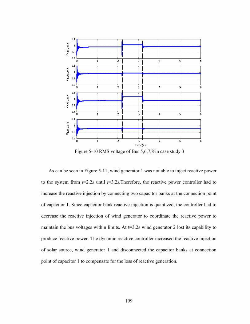
199

Figure 5-10 RMS voltage of Bus 5,6,7,8 in case study 3

As can be seen in Figure 5-11, wind generator 1 was not able to inject reactive power

to the system from t=2.2s until t=3.2s.Therefore, the reactive power controller had to

increase the reactive injection by connecting two capacitor banks at the connection point

of capacitor 1. Since capacitor bank reactive injection is quantized, the controller had to

decrease the reactive injection of wind generator to coordinate the reactive power to

maintain the bus voltages within limits. At t=3.2s wind generator 2 lost its capability to

produce reactive power. The dynamic reactive controller increased the reactive injection

of solar source, wind generator 1 and disconnected the capacitor banks at connection

point of capacitor 1 to compensate for the loss of reactive generation.

200

Vre

f

(p.u

.)Q

w1 (p

.u.)

Qw

2 (p

.u.)

QS

(p.u

.)Q

c1 (p

.u.)

Qc2

(p.u

.)



In this case-study, the same generation changes as case-study 3 occurred in the

system. However, D-STATCOMs were used for reactive power compensation instead of

capacitor banks. The problem formulation was the same as case-study 3, and the

optimization problem led into solving a QP problem. The voltage of the load buses are

shown in Figure 5-12 and the control inputs are depicted in Figure 5-13. Similar to

case-study 3, the dynamic reactive controller used alternative reactive capabilities of the

system to achieve smooth voltage profile when one reactive power source was

unavailable.

201

Figure 5-12 RMS voltage of Bus 5,6,7,8 in case study 4

As can be seen in Figure 5-13, wind generator 1 lost its capability to produce

reactive power at t=2.2s. Therefore, the dynamic reactive controller had to increase the

reactive power injection of the solar source and the voltage reference of the master

generator. These changes alone would cause overvoltage in some buses in the system.

Therefore, the reactive controller had to decrease the reactive injection of wind generator

2 and the D-STATCOMs. At t=3.2s, wind generator 2 lost its capability to produce

reactive power. Therefore, the dynamic reactive controller increased the reactive

injection of both reactive compensators as well as wind generator 1. In this case, the

reactive controller had to slightly decrease the reactive injection of the solar source. As

can be seen in Figure 5-12, these controller was able to maintain bus voltages within

limits taking these control actions.

202


5.5.2 Studies on IEEE 34 node MicroGrid

Figure 5-14 shows a MicroGrid based designed based on the IEEE34 node. The

system is divided into three zones and each zone contains a DER. The system was

designed such that the DERs were capable of providing active and reactive power to the

loads when the MicroGrid was operating in islanded mode. Two capacitor banks were

used as switched capacitor banks in the case-study which means that the general

controller was capable of connecting and disconnecting them.

203

Figure 5-14 MicroGrid based on the IEEE 34 node feeder

204

The distributed loads of the MicroGrid are listed in Table 16. The spot loads of the

MicroGrid are shown in Table 17. Source parameters of the MicroGrid shown in Figure

5-14 is are listed in Table 18.

Table 16 Distributed loads of the IEEE 34 node system

Node Node Load Ph-1 Ph-1 Ph-2 Ph-2 Ph-3 Ph-3 A B Model kW kVAr kW kVAr kW kVAr

802 806 Y-PQ 0 0 30 15 25 14 808 810 Y-I 0 0 16 8 0 0 818 820 Y-Z 34 17 0 0 0 0 820 822 Y-PQ 135 70 0 0 0 0 816 824 D-I 0 0 5 2 0 0 824 826 Y-I 0 0 40 20 0 0 824 828 Y-PQ 0 0 0 0 4 2 828 830 Y-PQ 7 3 0 0 0 0 854 856 Y-PQ 0 0 4 2 0 0 832 858 D-Z 7 3 2 1 6 3 858 864 Y-PQ 2 1 0 0 0 0 858 834 D-PQ 4 2 15 8 13 7 834 860 D-Z 16 8 20 10 110 55 860 836 D-PQ 30 15 10 6 42 22 836 840 D-I 18 9 22 11 0 0 862 838 Y-PQ 0 0 28 14 0 0 842 844 Y-PQ 9 5 0 0 0 0 844 846 Y-PQ 0 0 25 12 20 11 846 848 Y-PQ 0 0 23 11 0 0

Total 262 133 240 120 220 114

205

Table 17 Spot loads of the IEEE 34 node system Node Load Ph-1 Ph-1 Ph-2 Ph-2 Ph-3 Ph-3

Model kW kVAr kW kVAr kW kVAr 860 Y-PQ 20 16 20 16 20 16 840 Y-I 9 7 9 7 9 7 844 Y-Z 135 105 135 105 135 105 848 D-PQ 20 16 20 16 20 16 890 D-I 150 75 150 75 150 75 830 D-Z 10 5 10 5 25 10

Total 344 224 344 224 359 229

Table 18 Source parameters of the IEEE 34 node system

Diesel Quantity Wind Quantity

VgI-I 13.8 kV VgI-I 575V Pg 1MW Pg 0.75 MW pfg 0.85 Vs 575 V

f 60 Hz Vr 1975 V Ra 0.199Ω F 60 Hz Xp 0.18 Rs 0.023 (p.u.) Xd 1.305 Ls 0.18 (p.u.) Xd' 0.296 Rr 0.016 (p.u.) Xd'' 0.252 Lr 0.16 (p.u.) Tdo' 1.01s Lm 2.9 (p.u.) Tdo'' 0.053s H 0.685 (p.u.) Xq 0.474 f 0.01 (p.u.) Xq' N.A Poles 3 Xq'' 0.243 Tqo' N.A

Tqo'' 0.061s Pg (solar) 0.4 MW

H 1.06s f (solar) 60 Hz

The result of steady state load flow of the MicroGrid when the diesel generator was off and the MicroGrid was connected to the main grid is shown in Table 19 and Table 20. The result of steady state load flow of the MicroGrid when it was operating in the islanded mode is shown in

Table 21 and

Table 22.

206

Table 19 Power flow of the system when connected to the grid and the Diesel generator is off – Bus voltages

Voltage Voltage Angle

Bus A B C A B C

800 1.05 1.05 1.05 0.00 -118.97 119.96

802 1.05 1.05 1.05 -0.07 -119.04 119.89

806 1.05 1.05 1.05 -0.11 -119.08 119.85

808 1.04 1.04 1.04 -0.93 -119.88 119.01

810 1.04 1.04 1.04 -0.93 -119.88 119.01

812 1.02 1.03 1.03 -1.90 -120.84 118.02

814 1.01 1.02 1.02 -2.68 -121.62 117.21

850 1.01 1.02 1.02 -2.68 -121.62 117.21

816 1.01 1.02 1.02 -2.69 -121.63 117.20

818 1.01 1.02 1.02 -2.68 -121.63 117.20

820 1.01 1.02 1.01 -2.55 -121.63 117.07

822 1.01 1.02 1.01 -2.53 -121.63 117.05

824 1.01 1.01 1.01 -2.99 -121.92 116.95

826 1.01 1.01 1.01 -2.99 -121.92 116.95

828 1.01 1.01 1.01 -3.04 -121.97 116.90

830 0.99 0.99 0.99 -4.31 -123.24 115.72

854 0.99 0.99 0.99 -4.35 -123.28 115.69

856 0.99 0.99 0.99 -4.35 -123.28 115.69

852 0.95 0.95 0.95 -6.74 -125.67 113.48

832 0.95 0.95 0.95 -6.74 -125.67 113.48

888 1.05 1.05 1.05 -14.36 -133.23 106.13

890 0.90 0.90 0.90 -18.56 -137.42 102.08

858 0.95 0.95 0.95 -7.04 -125.97 113.20

864 0.95 0.95 0.95 -7.04 -125.97 113.20

834 0.95 0.95 0.95 -7.39 -126.33 112.87

842 0.95 0.95 0.95 -7.42 -126.35 112.85

844 0.95 0.95 0.95 -7.55 -126.48 112.73

846 0.95 0.95 0.95 -7.82 -126.74 112.47

848 0.95 0.95 0.95 -7.86 -126.78 112.43

860 0.95 0.95 0.95 -7.40 -126.33 112.87

836 0.95 0.95 0.95 -7.41 -126.34 112.87

862 0.95 0.95 0.95 -7.41 -126.34 112.87

838 0.95 0.95 0.95 -7.41 -126.34 112.87

840 0.95 0.95 0.95 -7.41 -126.34 112.87

207

Table 20 Power flow of the system when connected to the grid and the Diesel generator is off – Line currents

Current From Bus To Bus A B C

800 802 29.88 29.33 28.85 802 806 29.88 29.33 28.85 806 808 29.88 27.54 27.37 808 810 29.88 27.54 27.37 808 812 29.88 26.61 27.37 812 814 29.88 26.61 27.37 814 850 29.88 26.61 27.37 850 816 29.81 26.71 27.03 816 818 10.59 0.00 0.00 818 820 9.53 0.00 0.00 820 822 9.53 0.00 0.00 816 824 20.68 26.43 27.03 824 826 0.00 1.25 0.00 824 828 65.64 69.29 71.24 828 830 65.25 69.29 71.24 830 854 63.61 67.64 68.75 854 856 0.00 0.12 0.00 854 852 63.61 67.42 68.75 852 832 63.61 67.42 68.75 832 888 21.61 21.60 21.58 888 890 21.61 21.60 21.58 832 858 21.61 21.60 21.58 858 864 0.06 0.00 0.00 858 834 48.63 52.05 53.03 834 842 87.94 89.61 88.21 842 844 87.54 89.61 88.21 844 846 67.04 67.91 66.88 846 848 67.04 67.91 66.88 834 860 4.63 5.36 4.30 860 836 4.63 5.36 4.30 836 862 0.00 1.66 0.00 862 838 0.00 1.66 0.00 836 840 2.34 2.45 1.81

208

Table 21 Power flow of the system isolated from the grid – Bus voltages Voltage Voltage angle

Bus A B C A B C

800 1.05 1.05 1.06 0.00 -119.66 121.06

802 1.05 1.05 1.06 0.00 -119.66 121.06

806 1.05 1.05 1.06 0.00 -119.66 121.06

808 1.05 1.05 1.06 0.03 -119.64 121.06

810 1.05 1.05 1.06 0.03 -119.64 121.06

812 1.05 1.05 1.06 0.08 -119.61 121.06

814 1.05 1.06 1.06 0.12 -119.59 121.06

850 1.05 1.06 1.06 0.12 -119.59 121.06

816 1.05 1.06 1.06 0.10 -119.60 121.04

818 1.05 1.06 1.06 0.11 -119.60 121.04

820 1.05 1.06 1.05 0.24 -119.60 120.91

822 1.05 1.06 1.05 0.25 -119.60 120.89

824 1.05 1.05 1.05 -0.30 -120.02 120.67

826 1.05 1.05 1.05 -0.30 -120.02 120.67

828 1.04 1.05 1.05 -0.35 -120.08 120.62

830 1.02 1.02 1.02 -1.68 -121.49 119.31

854 1.02 1.02 1.02 -1.72 -121.52 119.28

856 1.02 1.02 1.02 -1.72 -121.53 119.28

852 0.98 0.98 0.98 -4.24 -124.19 116.80

832 0.98 0.98 0.98 -4.24 -124.19 116.80

888 1.07 1.07 1.08 -11.59 -131.84 109.26

890 0.93 0.93 0.93 -15.64 -136.05 105.08

858 0.98 0.98 0.98 -4.56 -124.53 116.48

864 0.98 0.98 0.98 -4.56 -124.53 116.48

834 0.97 0.97 0.98 -4.94 -124.93 116.11

842 0.97 0.97 0.98 -4.97 -124.96 116.08

844 0.97 0.97 0.98 -5.09 -125.09 115.96

846 0.97 0.97 0.97 -5.35 -125.36 115.69

848 0.97 0.97 0.97 -5.39 -125.40 115.66

860 0.97 0.97 0.98 -4.95 -124.94 116.10

836 0.97 0.97 0.98 -4.95 -124.94 116.10

862 0.97 0.97 0.98 -4.95 -124.94 116.10

838 0.97 0.97 0.98 -4.95 -124.94 116.10

840 0.97 0.97 0.98 -4.95 -124.94 116.10

209

Table 22 Power flow of the system isolated from the grid – Line currents Current

From Bus To Bus A B C 800 802 0.00 0.00 0.00

802 806 0.00 0.00 0.00

806 808 0.00 1.93 1.66

808 810 0.00 1.93 1.66

808 812 0.00 0.00 0.00

812 814 0.00 2.96 1.66

814 850 0.00 2.96 1.66

850 816 53.12 49.85 50.81

816 818 10.90 0.00 0.00

818 820 9.81 0.00 0.00

820 822 4.36 0.00 0.00

816 824 4.36 0.00 0.00

824 826 0.00 1.28 0.00

824 828 82.28 85.96 88.37

828 830 81.87 85.96 88.37

830 854 80.15 84.23 85.80

854 856 0.00 0.12 0.00

854 852 80.15 84.00 85.80

852 832 80.15 84.00 85.80

832 888 25.86 25.81 25.84

888 890 25.86 25.81 25.84

832 858 58.79 62.43 63.76

858 864 0.06 0.00 0.00

858 834 88.85 90.35 89.14

834 842 88.85 90.35 89.14

842 844 88.85 90.35 89.14

844 846 88.44 90.35 89.14

846 848 67.72 68.47 67.60

834 860 4.68 5.41 4.34

860 836 2.89 4.79 1.83

836 862 0.00 1.67 0.00

862 838 0.00 1.67 0.00

836 840 2.36 2.47 1.83

210

The objective function for reactive power control of the MicroGrid shown in Figure

5-14 was chosen as follows.

, , |,

∈

|,

|,

‖ ∆ ‖ , ‖ ∆ ‖ ,

(5-10)

where | , | , | are the predicted voltage of phase A, B

and C of bus i, respectively.

The control inputs to the system were the reference voltage of synchronous diesel

generator ( ), and reactive power setpoints of the DGs and the switched capacitors

( , ). Thus, the control input vectors were defined as follows.

, , , , (5-11)

Since the system had three distributed generators, and one dynamic load, the number

of the states of the system was four. So the optimization problem was solved subject to

the following simplified differential algebraic equations.

1 Δ1

1

(5-12)

211

1 Δ1

,,

,1

, , 2,3

(5-13)

1 Δ

(5-14)

(5-15)

| | 1, … . , | |

| || | 1, … ,

(5-16)

Following the linearization technique discussed in [111], system state space

equations were derived in the piecewise linear form as follows.

11

⋮1

(5-17)

The bus voltages can be described in compact form as follows.

1⋮

1

(5-18)

where is the vector of the voltages that are used in the optimization formulation and it

includes the voltage of all three buses in the system. Increasing the number of sets makes

212

the prediction of voltage more accurate; however, the optimization algorithm takes more

time to converge to the global minimum.

5.5.2.1 Case-study 1: Load change with local control

Sharp load changes during islanded operation can cause instability and oscillatory

voltage in the MicroGrid. Further, the on load tap changers are not fast enough to avoid

the effect of sharp load changes efficiently.

This case-study is demonstrating the effect of sharp load change in the islanded

MicroGrid with local voltage control and fixed capacitors. The exciter of the master

generator usually damps the voltage oscillations in time if the relays do not operate and

isolate the system any further. However, if the protection relays are triggered the system

may experience a blackout. Figure 5-15 and Figure 5-16 show the voltage oscillations

resulting from the load change in the system.

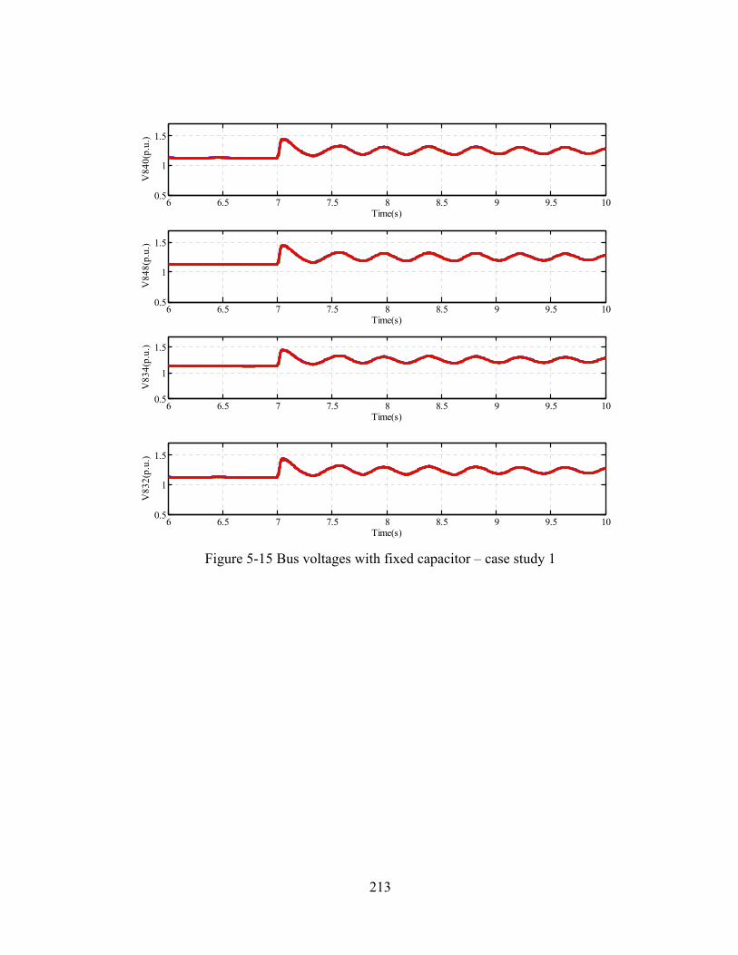
213

Figure 5-15 Bus voltages with fixed capacitor – case study 1

6 6.5 7 7.5 8 8.5 9 9.5 100.5

1

1.5

Time(s)

V84

0(p.

u.)

6 6.5 7 7.5 8 8.5 9 9.5 100.5

1

1.5

Time(s)

V84

8(p.

u.)

6 6.5 7 7.5 8 8.5 9 9.5 100.5

1

1.5

Time(s)

V83

2(p.

u.)

6 6.5 7 7.5 8 8.5 9 9.5 100.5

1

1.5

Time(s)

V83

4(p.

u.)

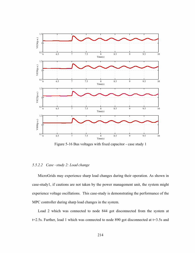
214

Figure 5-16 Bus voltages with fixed capacitor - case study 1

5.5.2.2 Case –study 2: Load change

MicroGrids may experience sharp load changes during their operation. As shown in

case-study1, if cautions are not taken by the power management unit, the system might

experience voltage oscillations. This case-study is demonstrating the performance of the

MPC controller during sharp load changes in the system.

Load 2 which was connected to node 844 got disconnected from the system at

t=2.5s. Further, load 1 which was connected to node 890 got disconnected at t=3.5s and

6 6.5 7 7.5 8 8.5 9 9.5 100.5

1

1.5

Time(s)

V82

4(p.

u.)

6 6.5 7 7.5 8 8.5 9 9.5 100.5

1

1.5

Time(s)

V85

0(p.

u.)

6 6.5 7 7.5 8 8.5 9 9.5 100.5

1

1.5

Time(s)

V82

2(p.

u.)

6 6.5 7 7.5 8 8.5 9 9.5 100.5

1

1.5

Time(s)

V80

0(p.

u.)

215

both of the loads were energized again at t=5.5s. The generalized MPC controller tried to

reduce the effect of the load change in the system by sending optimal control inputs to

the system. The assumption in this case-study was that the MPC controller does not have

a prediction of the exact time of load change. Therefore, after the load status changed, it

took 0.2 seconds for the controller to send the updated control inputs to the system. As

can be seen in Figure 5-17 and Figure 5-18, the MPC controller was able to keep the

voltages within the limits by adjusting the control input.

Each of loads 1 and 2 are approximately 25% of the system’s total load. Given that

the load change was significantly large in this case-study and the system was operating

in islanded mode, the bus voltage experience a spike immediately after the voltage

change. This transient behavior is acceptable with current requirements presented in

IEEE Standard for isolated power systems [106]. The IEEE Std 1547.4 mentions that the

under-voltage tripping time are 0.16s for voltage less than 50% and 2s for voltages less

than 88%. In this case-study, the variations in the voltage beyond the 12% limit occurred

for less than 0.2 seconds, which is acceptable according to IEEE 1547.4 Standard for

isolated power systems and does not cause relays to trip.

216

Figure 5-17 Bus voltages with MPC – case study 2

1 2 3 4 5 6 7 8

0.6

0.8

1

1.2

Time(s)

V84

0(p.

u.)

1 2 3 4 5 6 7 8

0.6

0.8

1

1.2

Time(s)

V84

8(p.

u.)

1 2 3 4 5 6 7 8

0.6

0.8

1

1.2

Time(s)

V83

4(p.

u.)

1 2 3 4 5 6 7 8

0.6

0.8

1

1.2

Time(s)

V83

2(p.

u.)

217


Figure 5-19 shows how the proposed dynamic reactive controller coordinated the

reactive power sources in the system to achieve the optimal solution. After the first load

change at t=2.5s, the controller responded by decreasing the local reactive power

injection of the wind generators. After the second load change, the controller responded

by disconnecting the capacitor banks from the system, increasing the reactive injection

of the wind generators, and increasing the voltage reference of the master generator. It

1 2 3 4 5 6 7 8

0.6

0.8

1

1.2

Time(s)

V82

4(p.

u.)

1 2 3 4 5 6 7 8

0.6

0.8

1

1.2

Time(s)

V85

0(p.

u.)

1 2 3 4 5 6 7 8

0.6

0.8

1

1.2

Time(s)

V82

2(p.

u.)

1 2 3 4 5 6 7 8

0.6

0.8

1

1.2

Time(s)

V80

0(p.

u.)

218

should be noted that disconnecting the capacitor banks alone would have resulted in an

overvoltage in the system. On the other hand, the controller could not keep the bus

voltages within limits without turning the capacitor banks off.

Figure 5-19 Control inputs to the MicroGrid generated by MPC – case study 2

1 2 3 4 5 6 7 80.9

1

1.1

Time(s)

Vre

f(p.

u.)

1 2 3 4 5 6 7 8-0.2

0

0.2

Time(s)

Qw

1(p.

u.)

1 2 3 4 5 6 7 8-0.2

0

0.2

Time(s)

Qw

2(p.

u.)

1 2 3 4 5 6 7 80

0.5

1

Time(s)

Qc1

1 2 3 4 5 6 7 80

0.5

1

Time(s)

Qc2

219

5.5.2.3 Case –study 3: Wind change

In this case-study, the wind speed changed to 60% of rated speed from t=4s to t=15s.

The variations in wind speed resulted in variation in the output power of the wind

generator. Wind speed variations may affect the stability of the system as well as the

voltage level of the load buses. The model predictive control had an estimate of the wind

variation, which is provided by the user based on the weather forecast. This forecast

does not need to be exactly accurate and the reactive controller can operate as long as it

can estimate the reactive power injection capacity of the wind sources. The controller

had to determine what percentage of the output power may be assigned to reactive power

generation based on the total generated power of the wind generator. The reactive power

generation limit of the wind generator was tighter in this case, so reactive power had to

be provided by other sources of reactive power in the system.

The bus voltages of some buses in the system are shown in Figure 5-20and Figure

5-21. The system also experiences a temporary fault at t=8.5s which results in a glitch in

bus voltages.

220

Figure 5-20 Bus voltages of MicroGrid – case study 3

5 10 15 20 25

0.6

0.8

1

1.2

Time(s)V

840(

p.u.

)

5 10 15 20 25

0.6

0.8

1

1.2

Time(s)

V84

8(p.

u.)

5 10 15 20 25

0.6

0.8

1

1.2

Time(s)

V83

4(p.

u.)

5 10 15 20 25

0.6

0.8

1

1.2

Time(s)

V83

2(p.

u.)

221

Figure 5-21 Bus voltages of the MicroGrid – case study 3

As can be seen in Figure 5-22, the reactive controller lowered the reactive power

reference of the wind generators and increased the voltage setpoint of the master

generator. Increasing the voltage setpoint of the master generator resulted in a bus

voltage increase in all the buses of the microgrid. This is a wasteful method to keep bus

voltage within limits and it puts stress on the diesel generator. However, in this case, the

controller does not have access to any other local reactive injectors.

5 10 15 20 25

0.6

0.8

1

1.2

Time(s)

V82

4(p.

u.)

5 10 15 20 25

0.6

0.8

1

1.2

Time(s)

V85

0(p.

u.)

5 10 15 20 25

0.6

0.8

1

1.2

Time(s)

V82

2(p.

u.)

5 10 15 20 25

0.6

0.8

1

1.2

Time(s)

V80

0(p.

u.)

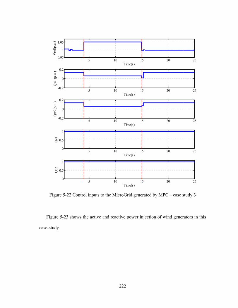
222


Figure 5-23 shows the active and reactive power injection of wind generators in this

case-study.

5 10 15 20 250.95

1

1.05

Time(s)

Vre

f(p.

u.)

5 10 15 20 25-0.2

0

0.2

Time(s)

Qw

1(p.

u.)

5 10 15 20 25-0.2

0

0.2

Time(s)

Qw

2(p.

u.)

5 10 15 20 250

0.5

1

Time(s)

Qc1

5 10 15 20 250

0.5

1

Time(s)

Qc2

223

Figure 5-23 Active and reactive power generation of the wind generators – case study 3

5.5.2.4 Case-study 4: Motor starting

In this case-study, all the loads of the IEEE 34 node system were connected to the

system. The induction motor connected to bus 840 started operating at t=2s and drew the

starting current for about one second. The MPC controller used the available control

inputs to achieve the voltage goals, but was still not capable of providing the extra

voltage and reactive support to keep the bus voltage within limits during the motor

5 10 15 20 25

0.6

0.8

1

1.2

Time(s)

Pw

1(p.

u.)

5 10 15 20 25-0.1

0

0.1

0.2

Time(s)

Qw

1(p.

u.)

5 10 15 20 25

0.6

0.8

1

1.2

Time(s)

Pw

2(p.

u.)

5 10 15 20 25-0.1

0

0.1

0.2

Time(s)

Qw

2(p.

u.)

224

startup. This is normal in most induction motor startups in heavily loaded power

systems.

Figure 5-24, Figure 5-25 shows the bus voltages dropped below the requirement

during motor startup. This drop did not make the system go unstable or the relays to trip.

However, this voltage drop can result in flickering lights in the distribution system.


1 2 3 4 5 6 7

0.6

0.8

1

1.2

Time(s)

V82

4(p.

u.)

1 2 3 4 5 6 7

0.6

0.8

1

1.2

Time(s)

V85

0(p.

u.)

1 2 3 4 5 6 7

0.6

0.8

1

1.2

Time(s)

V82

2(p.

u.)

1 2 3 4 5 6 7

0.6

0.8

1

1.2

Time(s)

V80

0(p.

u.)

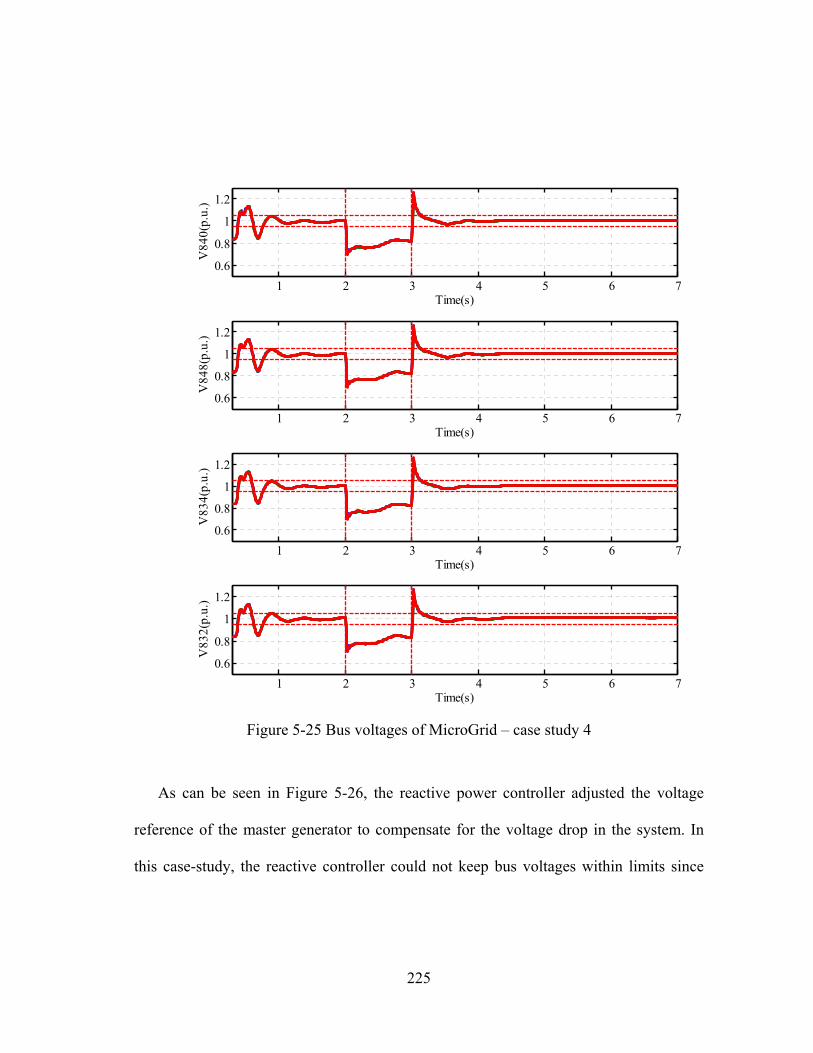
225


As can be seen in Figure 5-26, the reactive power controller adjusted the voltage

reference of the master generator to compensate for the voltage drop in the system. In

this case-study, the reactive controller could not keep bus voltages within limits since

1 2 3 4 5 6 7

0.6

0.8

1

1.2

Time(s)

V84

0(p.

u.)

1 2 3 4 5 6 7

0.6

0.8

1

1.2

Time(s)

V84

8(p.

u.)

1 2 3 4 5 6 7

0.6

0.8

1

1.2

Time(s)

V83

4(p.

u.)

1 2 3 4 5 6 7

0.6

0.8

1

1.2

Time(s)

V83

2(p.

u.)

226

there were no additional reactive capabilities in the system to inject reactive power

locally.

Figure 5-26 Control inputs to the MicroGrid – case study 4

5.5.2.5 Case-study 5: Induction motor starting and demand-response

In this case-study, all the loads of the IEEE 34 node system were connected to the

system. The spot load connected to bus 890 was considered a non-sensitive load that had

1 2 3 4 5 6 71

1.05

Time(s)

Vre

f(p.

u.)

1 2 3 4 5 6 7-0.2

0

0.2

Time(s)

Qw

1(p.

u.)

1 2 3 4 5 6 7-0.2

0

0.2

Time(s)

Qw

2(p.

u.)

1 2 3 4 5 6 70

0.5

1

Time(s)

Qc1

1 2 3 4 5 6 70

0.5

1

Time(s)

Qc2

227

a demand response contract with the utility. The induction motor connected to bus 840

started operating at t=2s and drew the starting current for about one second. The MPC

controller used the available control inputs to achieve the voltage goals. The control

signals generated by the MPC controller are depicted in Figure 5-27. As can be seen in

Figure 5-28 and Figure 5-29, the MPC controller used the demand response load to

reduce the reactive power consumption of the whole system, which resulted in less

voltage drop in the buses comparing to case-study 4.

Compared to case-study 5, in this case the controller also disconnected the demand-

response load during the startup period of the motor. The demand-response load was

disconnected when QDR=1 and connected when QDR=0 Disconnecting the demand-

response load resulted in a less voltage drop in the buses in the system. The voltage of

some buses are depicted in Figure 5-28, Figure 5-29.

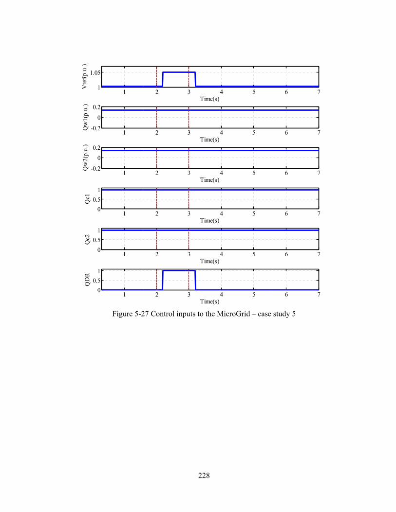
228


1 2 3 4 5 6 71

1.05

Time(s)

Vre

f(p.

u.)

1 2 3 4 5 6 7-0.2

0

0.2

Time(s)

Qw

1(p.

u.)

1 2 3 4 5 6 7-0.2

0

0.2

Time(s)

Qw

2(p.

u.)

1 2 3 4 5 6 70

0.5

1

Time(s)

Qc1

1 2 3 4 5 6 70

0.5

1

Time(s)

Qc2

1 2 3 4 5 6 70

0.5

1

Time(s)

QD

R

229


1 2 3 4 5 6 7

0.6

0.8

1

1.2

Time(s)

V82

4(p.

u.)

1 2 3 4 5 6 7

0.6

0.8

1

1.2

Time(s)

V85

0(p.

u.)

1 2 3 4 5 6 7

0.6

0.8

1

1.2

Time(s)

V82

2(p.

u.)

1 2 3 4 5 6 7

0.6

0.8

1

1.2

Time(s)

V80

0(p.

u.)

230


5.5.2.6 Case-study 6: Motor starting with demand-response

In this case-study, the spot load at 844 was disconnected from the system all through

the case-study. The induction motor connected to bus 840 started operating at t=2s and

drew the starting current for about one second. A non-sensitive load with a demand-

response contract with the utility was connected at bus 890. The MPC controller used the

available control inputs to achieve the voltage goals. Figure 5-30and Figure 5-31 show

1 2 3 4 5 6 7

0.6

0.8

1

1.2

Time(s)

V84

0(p.

u.)

1 2 3 4 5 6 7

0.6

0.8

1

1.2

Time(s)

V84

8(p.

u.)

1 2 3 4 5 6 7

0.6

0.8

1

1.2

Time(s)

V83

4(p.

u.)

1 2 3 4 5 6 7

0.6

0.8

1

1.2

Time(s)

V83

2(p.

u.)

231

that compared to case-study 4 and 5, the controller was more successful in keeping the

voltage close to required level during motor startup. During the transient condition, the

system experienced voltage spikes and voltage drops. As mentioned earlier, the present

requirements in IEEE Std 1547.4 [106] for under-voltage tripping time are 0.16 s for

voltage less than 50% and 2 s for voltages less than 88%. The variations in the voltage

beyond the 12% limit occurred for less than 0.2 seconds, which is acceptable according

to IEEE 1547.4 Standard for isolated power systems and does not cause relays to trip.

Some bus voltages remained outside the 5% limit for around one second.

As can be seen in Figure 5-32, the MPC controller increased the reference voltage of

the master generator, disconnected the DR load, and connected the capacitor bank to be

able to provide enough reactive power for the induction motor startup.

232


1 2 3 4 5 6 7

0.6

0.8

1

1.2

Time(s)

V84

0(p.

u.)

1 2 3 4 5 6 7

0.6

0.8

1

1.2

Time(s)

V84

8(p.

u.)

1 2 3 4 5 6 7

0.6

0.8

1

1.2

Time(s)

V83

4(p.

u.)

1 2 3 4 5 6 7

0.6

0.8

1

1.2

Time(s)

V83

2(p.

u.)

233


1 2 3 4 5 6 7

0.6

0.8

1

1.2

Time(s)

V82

4(p.

u.)

1 2 3 4 5 6 7

0.6

0.8

1

1.2

Time(s)

V85

0(p.

u.)

1 2 3 4 5 6 7

0.6

0.8

1

1.2

Time(s)

V82

2(p.

u.)

1 2 3 4 5 6 7

0.6

0.8

1

1.2

Time(s)

V80

0(p.

u.)

234


5.5.2.7 Case-study 7: Induction starting with demand response and increasing reactive

support

In this case-study, the spot load at 844 was disconnected from the system all through

the case-study. The induction motor connected to bus 840 started operating at t=2s and

1 2 3 4 5 6 71

1.05

Time(s)

Vre

f(p.

u.)

1 2 3 4 5 6 7-0.2

0

0.2

Time(s)

Qw

1(p.

u.)

1 2 3 4 5 6 7-0.2

0

0.2

Time(s)

Qw

2(p.

u.)

1 2 3 4 5 6 70

0.5

1

Time(s)

Qc1

1 2 3 4 5 6 70

0.5

1

Time(s)

Qc2

1 2 3 4 5 6 70

0.5

1

Time(s)

QD

R

235

drew the starting current for about one second. A non-sensitive load with demand

response contract with the utility was connected to bus 890.

In this case-study, when the demand response load was disconnected from the

system, the PQ generators in the system had higher reactive power production capacity,

since less active power was being consumed by the loads in the system. Thus, the MPC

controller adjusted the reactive power production limit of the wind generators. Figure

5-33 shows how the reactive power controller increased the reactive power production

setpoint of the wind generator to achieve the voltage requirements. Similar to the

previous case-study, the reactive power controller increased the voltage reference of the

master generator and disconnected the demand-response load. As can be seen in Figure

5-34 and Figure 5-35, the MPC controller was able to maintain the voltage within limits

in this case with proper adjustment and demand-response load. In this case the system

only experiences voltage drop and voltage spike for short periods of time. The light

flickering in the distribution system is not visible in that short duration. Compared to

case-study 4,5, and 6, the controller performed better in case-study since it had more

flexibility in terms of control inputs to achieve the required criteria.

236


1 2 3 4 5 6 71

1.05

Time(s)

Vre

f(p.

u.)

1 2 3 4 5 6 70

0.1

0.2

Time(s)

Qw

1(p.

u.)

1 2 3 4 5 6 70

0.1

0.2

Time(s)

Qw

2(p.

u.)

1 2 3 4 5 6 70

0.5

1

Time(s)

Qc1

1 2 3 4 5 6 70

0.5

1

Time(s)

Qc2

1 2 3 4 5 6 70

0.5

1

Time(s)

QD

R

237


1 2 3 4 5 6 7

0.6

0.8

1

1.2

Time(s)

V82

4(p.

u.)

1 2 3 4 5 6 7

0.6

0.8

1

1.2

Time(s)

V85

0(p.

u.)

1 2 3 4 5 6 7

0.6

0.8

1

1.2

Time(s)

V82

2(p.

u.)

1 2 3 4 5 6 7

0.6

0.8

1

1.2

Time(s)

V80

0(p.

u.)

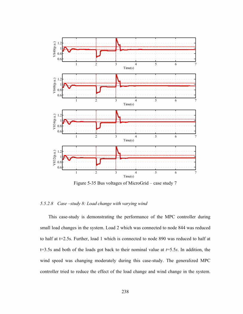
238


5.5.2.8 Case –study 8: Load change with varying wind

This case-study is demonstrating the performance of the MPC controller during

small load changes in the system. Load 2 which was connected to node 844 was reduced

to half at t=2.5s. Further, load 1 which is connected to node 890 was reduced to half at

t=3.5s and both of the loads got back to their nominal value at t=5.5s. In addition, the

wind speed was changing moderately during this case-study. The generalized MPC

controller tried to reduce the effect of the load change and wind change in the system.

1 2 3 4 5 6 7

0.6

0.8

1

1.2

Time(s)

V84

0(p.

u.)

1 2 3 4 5 6 7

0.6

0.8

1

1.2

Time(s)

V84

8(p.

u.)

1 2 3 4 5 6 7

0.6

0.8

1

1.2

Time(s)

V83

4(p.

u.)

1 2 3 4 5 6 7

0.6

0.8

1

1.2

Time(s)

V83

2(p.

u.)

239

The assumption in this case-study was that the MPC controller did not have a prediction

of the exact time of load change. Therefore, after the load changed, it took 0.3 seconds

for the controller to send the updated control inputs to the system since the step time of

the control algorithm was set to 0.3s. As can be seen in Figure 5-37 and Figure 5-38, the

MPC controller was able to keep the voltages within the limits by adjusting the control

inputs. In this case-study, to reduce the losses in the system and to reduce the peak

power, the reference voltage setpoint was chosen equal to 0.96 p.u. The wind profile in

this case-study is shown in Figure 5-36.

Figure 5-36 Wind profile

0 1 2 3 4 5 6 7 813

13.5

14

14.5

15

Time(s)

win

d sp

eed

(m/s

)

240


1 2 3 4 5 6 7 8

0.6

0.8

1

1.2

Time(s)

V84

0(p.

u.)

1 2 3 4 5 6 7 8

0.6

0.8

1

1.2

Time(s)

V84

8(p.

u.)

1 2 3 4 5 6 7 8

0.6

0.8

1

1.2

Time(s)

V83

4(p.

u.)

1 2 3 4 5 6 7 80.5

1

Time(s)

V83

2(p.

u.)

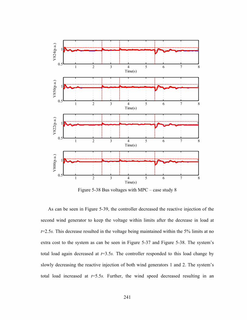
241


As can be seen in Figure 5-39, the controller decreased the reactive injection of the

second wind generator to keep the voltage within limits after the decrease in load at

t=2.5s. This decrease resulted in the voltage being maintained within the 5% limits at no

extra cost to the system as can be seen in Figure 5-37 and Figure 5-38. The system’s

total load again decreased at t=3.5s. The controller responded to this load change by

slowly decreasing the reactive injection of both wind generators 1 and 2. The system’s

total load increased at t=5.5s. Further, the wind speed decreased resulting in an

1 2 3 4 5 6 7 80.5

1

Time(s)

V82

4(p.

u.)

1 2 3 4 5 6 7 80.5

1

Time(s)

V85

0(p.

u.)

1 2 3 4 5 6 7 80.5

1

Time(s)

V82

2(p.

u.)

1 2 3 4 5 6 7 80.5

1

Time(s)

V80

0(p.

u.)

242

additional demand for reactive support. The designed controller responded by increasing

the reactive injection of both wind generators. The controller also increased the voltage

reference of the master generator for a short period of time. These changes in the control

input resulted in the voltages of the system to stay within the 5% limits except for a very

short period as can be seen in Figure 5-37 and Figure 5-38.


1 2 3 4 5 6 7 80.9

1

1.1

Time(s)

Vre

f(p.

u.)

1 2 3 4 5 6 7 8-0.2

0

0.2

Time(s)

Qw

1(p.

u.)

1 2 3 4 5 6 7 8-0.2

0

0.2

Time(s)

Qw

2(p.

u.)

1 2 3 4 5 6 7 80

0.5

1

Time(s)

Qc1

1 2 3 4 5 6 7 80

0.5

1

Time(s)

Qc2

243

5.5.2.9 Case –study 9: Controller failure due to capacitor bank malfunction

This case-study is demonstrating the effect of malfunction of the actuators of the

components on the performance the MPC controller during sharp load changes in the

system. Load 2 which was connected to node 844 got disconnected from the system at

t=2.5s. Further, load 1 which was connected to node 890 got disconnected at t=3.5s and

both of the loads were energized again at t=5.5s. The generalized MPC controller tried to

reduce the effect of the load change in the system by sending optimal control inputs to

the system. The assumption in this case-study was that the MPC controller does not have

a prediction of the exact time of load change. Therefore, after the load changed, it took

0.2 seconds for the controller to send the updated control inputs to the system. After the

load change at t=3.5s, the controller tried to disconnect the capacitor banks one by one to

coordinate the reactive power in the system. However, the actuators of the capacitor

banks malfunctioned, which resulted in the capacitor banks to remain connected to the

system. As a result the MicroGrid buses experienced an overvoltage for a few seconds as

can be seen in Figure 5-40 and Figure 5-41. This overvoltage can be destructive to the

system and cause insulation damaging.

244


1 2 3 4 5 6 7 80.5

1

Time(s)V

824(

p.u.

)

1 2 3 4 5 6 7 80.5

1

Time(s)

V85

0(p.

u.)

1 2 3 4 5 6 7 80.5

1

Time(s)

V82

2(p.

u.)

1 2 3 4 5 6 7 80.5

1

Time(s)

V80

0(p.

u.)

245


The control inputs to the system in case-study 9 are depicted in Figure 5-42.

1 2 3 4 5 6 7 80.5

1

Time(s)

V84

0(p.

u.)

1 2 3 4 5 6 7 80.5

1

Time(s)

V84

8(p.

u.)

1 2 3 4 5 6 7 80.5

1

Time(s)

V83

4(p.

u.)

1 2 3 4 5 6 7 80.5

1

Time(s)

V83

2(p.

u.)

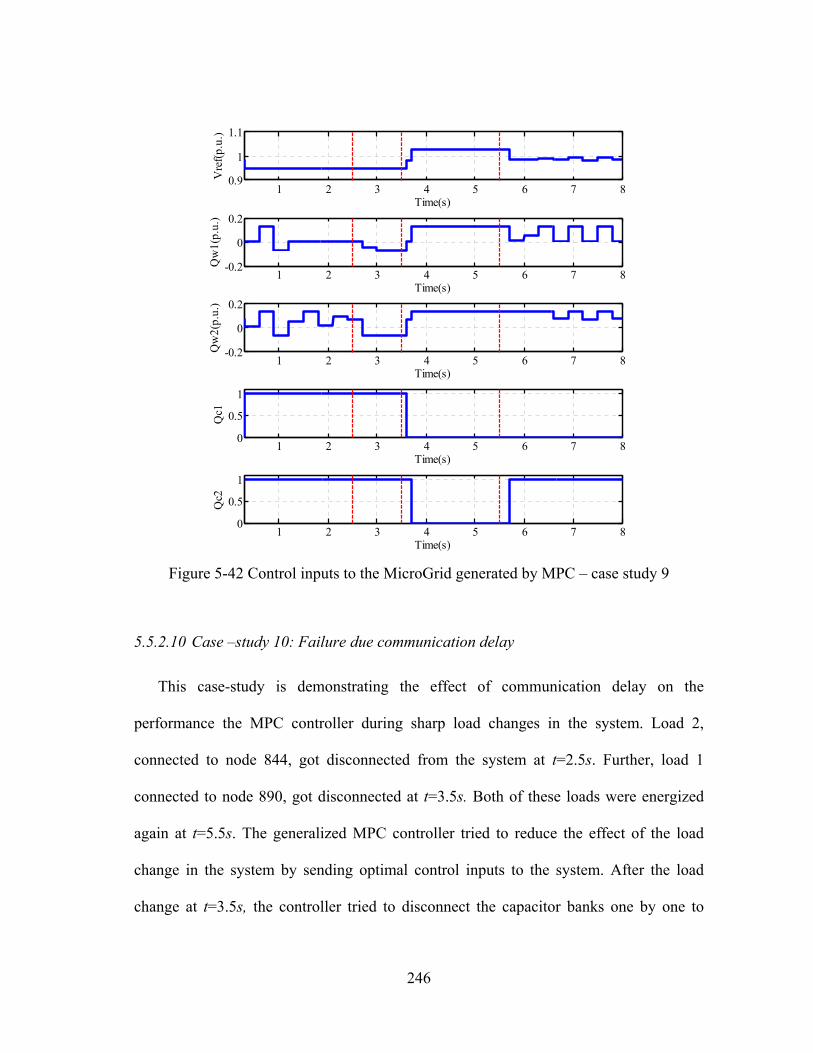
246


5.5.2.10 Case –study 10: Failure due communication delay

This case-study is demonstrating the effect of communication delay on the

performance the MPC controller during sharp load changes in the system. Load 2,

connected to node 844, got disconnected from the system at t=2.5s. Further, load 1

connected to node 890, got disconnected at t=3.5s. Both of these loads were energized

again at t=5.5s. The generalized MPC controller tried to reduce the effect of the load

change in the system by sending optimal control inputs to the system. After the load

change at t=3.5s, the controller tried to disconnect the capacitor banks one by one to

1 2 3 4 5 6 7 80.9

1

1.1

Time(s)V

ref(

p.u.

)

1 2 3 4 5 6 7 8-0.2

0

0.2

Time(s)

Qw

1(p.

u.)

1 2 3 4 5 6 7 8-0.2

0

0.2

Time(s)

Qw

2(p.

u.)

1 2 3 4 5 6 7 80

0.5

1

Time(s)

Qc1

1 2 3 4 5 6 7 80

0.5

1

Time(s)

Qc2

247

coordinate the reactive power in the system. However, the communication between the

centralized controller and the capacitor banks experienced 1 second delay. This

communication delay resulted in an overvoltage for around one second and an abnormal

behavior in the system voltages as can be seen in Figure 5-43and Figure 5-44. In

addition, the controller tried to connect the capacitor banks back to the system after the

load change at t=5.5s. The system experienced the same communication delay for one

second resulting in an undervoltage in the system buses for one second.


1 2 3 4 5 6 7 8

0.6

0.8

1

1.2

Time(s)

V82

4(p.

u.)

1 2 3 4 5 6 7 8

0.6

0.8

1

1.2

Time(s)

V85

0(p.

u.)

1 2 3 4 5 6 7 8

0.6

0.8

1

1.2

Time(s)

V82

2(p.

u.)

1 2 3 4 5 6 7 8

0.6

0.8

1

1.2

Time(s)

V80

0(p.

u.)

248


The control inputs to the system in case-study 10 are depicted in Figure 5-45.

1 2 3 4 5 6 7 8

0.6

0.8

1

1.2

Time(s)

V84

0(p.

u.)

1 2 3 4 5 6 7 8

0.6

0.8

1

1.2

Time(s)

V84

8(p.

u.)

1 2 3 4 5 6 7 8

0.6

0.8

1

1.2

Time(s)

V83

4(p.

u.)

1 2 3 4 5 6 7 8

0.6

0.8

1

1.2

Time(s)

V83

2(p.

u.)

249


5.6 Summary

This section discussed reactive power and voltage control of the MicroGrid. The

problem was formulated considering the dynamics of the MicroGrid. MATLAB and

CPLEX were used to implement the method. Finally, some case-studies were presented

to show the effectiveness of the algorithm.

1 2 3 4 5 6 7 80.9

1

1.1

Time(s)V

ref(

p.u.

)

1 2 3 4 5 6 7 8-0.2

0

0.2

Time(s)

Qw

1(p.

u.)

1 2 3 4 5 6 7 8-0.2

0

0.2

Time(s)

Qw

2(p.

u.)

1 2 3 4 5 6 7 80

0.5

1

Time(s)

Qc1

1 2 3 4 5 6 7 80

0.5

1

Time(s)

Qc2

250

6 CONCLUSIONS AND FUTURE WORK

6.1 Conclusions

This dissertation presented a dynamic reactive control approach to control isolated

power systems. Isolated power systems are vulnerable to changes in loads or generation

and can easily get unstable. The reactive power control problem is a nonlinear problem

integrating discrete inputs. This work proposed using model predictive control for

reactive control of isolated systems. The system was linearized using a piecewise linear

approach. Then the piecewise linear model was unified in the MLD framework.

Replacing the nonlinearities by piecewise linear approximation introduces very small

modeling error. The modeling error hardly manifests itself in the control experiments

thus proving the usefulness of the MLD modeling approach. This dissertation showed

that the bus voltages can be stabilized by an MPC controller using only nominal control

moves. Tuning of the MPC controller is straightforward and systematic. The MPC

controller can effectively use discrete inputs such as capacitor banks and

Demand/Response loads as well as continuous inputs such as setpoint of dynamic

reactive compensators and DGs to achieve smooth bus voltage profile.

The study in this dissertation concludes that if the communication and control

infrastructure is available, MPC based reactive power control is viable option. MPC

requires a model of the system to be able to predict the behavior of the system ahead of

time; however, the model can be as simple as reactive power balance equations. The

study in this dissertation used a simplified reactive power flow model in MPC and the

simplified model achieved satisfactory results.

251

The author believes that in scope of 10-20 years, model predictive methods replace

the current control scheme of power systems not only in reactive control but also in

protection, and active power dispatch. The inherent robustness and reliability of MPC

controllers can adequately deal with the changing structure of power systems. To

achieve this goal, communication and control infrastructures of power systems need to

be improved. In addition, accurate measurements of power system in certain buses

should be available. With current trend in development of smart-grid and adding smart-

meters to power systems, these measurements will be available to the operator in the

distribution systems of the next decade.

6.2 Future Research

This dissertation only focused on dynamic reactive control of power systems. The

major assumption in this dissertation was that the active power loop is already designed

and works cooperatively with the reactive power control loop. Active and reactive power

control loops are usually studied separately in power systems. It is interesting to design a

dynamic active control loop using model predictive control and try to operate the two

loops together. Further, it is interesting to try design a controller that can control active

and reactive power together using one loop.

A challenge that the design in this dissertation faced was that the MPC resulted in

too much control action in some cases. To the knowledge of the author, MPC usually

results in more control action than other control methods. It is interesting to investigate

methods to penalize control action over a long horizon of time. Penalizing the control

action over a long horizon can help MPC to avoid too much control action. Another

252

challenge that this work experience was that from a control point of view the model

complexity was unnecessarily increased when a large number of binary variables were

associated with the approximations. As a result, the computation time for solving the

underlying MILP or MIQP problems became relatively large. The method used in this

dissertation was to limit the number of sectors in the piecewise linear system. In other

words, the piecewise linear system was limited to a small number of pieces. Other

methods can be further investigated to address the computation time increase. Since

most current designs and testbeds of MicroGrids and shipboard power systems do not

include an On-Load Tap Changer (OLTC), this dissertation did not focus on OLTCs.

Adding OLTCs as a control input to the control problem can be further investigated.

It is common in industry that the utility desired to pick a sub-optimal solution to the

reactive problem at the cost of not making too many changes in the system. In other

words, sometimes utilities prefer to only change the status of one component and

achieve a suboptimal solution. This approach slows down the aging of components in

the system. This dissertation did not focus on such an approach; however, the method

presented in this dissertation can be easily expanded to include such constraints.

253

REFERENCES

[1] J. D. Kueck, D. T. Rizy, F. Li, Y. Xu, H. Li, S. Adhikari, and P. Irminger, "Local

dynamic reactive power for correction of system voltage problems," Oak Ridge

National Laboratory, ORNL/TM-2008/174, 2008.

[2] E. Fuchs and M. Masoum, Power Quality in Power Systems and Electrical

Machines Academic Press, 2008.

[3] C. J. Dafis, "An observability formulation for nonlinear power systems modeled

as differential algebraic systems," Ph.D. dissertation, Dept. Elect. Eng., Drexel

University, 2005.

[4] F. Katiraei and M. R. Iravani, "Power management strategies for a Microgrid

with multiple distributed generation units," IEEE Trans. Power Syst., vol. 21, pp.

1821-1831, Nov. 2006.

[5] K. L. Butler, N. D. R. Sarma, and V. Ragendra Prasad, "Network reconfiguration

for service restoration in shipboard power distribution systems," IEEE Trans.

Power Syst., vol. 16, pp. 653-661, Nov. 2001.

[6] G. Gates, D. Shipp, and W. Vilcheck, "Electrical distribution system analysis for

off-shore oil production facilities," in Proc. Annual Petroleum and Chemical

Industry Conf., 1998, pp. 129-137.

[7] F. McNamara, "Optimising unit commitment in an island power system," in

Proc. IEE Colloquium on Effective Response of a Public Electricity Network to

Independent Generators, 1993, pp. 1-7.

254

[8] W. Wei, W. Daifeng, A. Arapostathis, and K. Davey, "Optimal power generation

scheduling of a shipboard power system," in Proc. IEEE Elect. Ship Tech. Symp.,

2007, pp. 519-522.

[9] S. Kulkarni and S. Santoso, "Estimating transient response of simple AC and DC

shipboard power systems to pulse load operations," in Proc. IEEE Conf. Electric

Ship Technologies Symp., 2009, pp. 73-78.

[10] C. Yan, G. K. Venayagamoorthy, and K. Corzine, "AIS-based coordinated and

adaptive control of generator excitation systems for an electric ship," IEEE

Trans. Indust. Electron., vol. 59, pp. 3102-3112, Aug. 2012.

[11] J. D. Kueck, R. H. Staunton, S. D. Labinov, and B. J. Kirby, "Microgrid energy

management system," Oak Ridge National Laboratory, P500-03-091F, 2003.

[12] J. Stevens, "Characterization of microgrids in the United States," Sandia National

Laboratories, Vienna, Virginia, 2005.

[13] D. Salomonsson, "Modeling, control and protection of low-voltage DC

Microgrids," Ph.D. dissertation, Dept. Elect. Eng., KTH University, Stockholm,

2008.

[14] M. Innorta, P. Marannino, G. P. Granelli, M. Montagna, and A. Silvestri,

"Security constrained dynamic dispatch of real power for thermal groups," IEEE

Trans. Power Syst., vol. 3, pp. 774-781, May 1988.

[15] Eltra, "Specifications for connecting wind farms to the transmission network,"

Eltra doc. no. 74174, 2000, available at:

http://www.offshorecenter.dk/log/bibliotek/Specifications-Eltra.pdf.

255

[16] S. Morozumi, "Micro-grid demonstration projects in Japan," in Proc. Power

Conversion Conf., 2007, pp. 635-642.

[17] T. Funabashi and R. Yokoyama, "Microgrid field test experiences in Japan," in

Proc. IEEE Power Eng. Soc. General Meeting, 2006, p. 2 pp.

[18] T. Geyer, "Low complexity model predictive control in power electronics and

power systems," Ph.D. dissertation, Dept. Elect. Eng., ETH Zurich University,

2005.

[19] M. Barnes, "An evaluation of Microgrid structures and their relative merits," in

Proc. IET Power Conv., 2007, pp. 1-34.

[20] N. Hatziargyriou, H. Asano, R. Iravani, and C. Marnay, "Microgrids - an

overview of ongoing research, development, and demonstration projects," IEEE

Power & Energy Mag., vol. 5, pp. 78-94, 2007.

[21] I. Roytelman, B. K. Wee, and R. L. Lugtu, "Volt/Var control algorithm for

modern distribution management system," IEEE Trans. Power Syst., vol. 10, pp.

1454-1460, Aug. 1995.

[22] J. Dréo, A. Pétrowski, P. Siarry, and E. Taillard, Metaheuristics for hard

optimization: Methods and case studies, 1 ed. Berlin, Germany: Springer-Verlag,

2006.

[23] Y. C. Huang, H. T. Yang, and C. L. Huang, "Solving the capacitor placement

problem in a radial distribution system using tabu search approach," IEEE Trans.

Power Syst., vol. 4, pp. 1868-1873, Nov. 1996.

256

[24] D. E. Goldberg, Genetic Algorithms in Search, Optimization, and Machine

Learning, 1 ed. Boston, MA: Addison-Wesley Professional, 1989.

[25] Y. d. Valle, S. Mohagheghi, J. C. Hernandez-Mejia, G. K. Venayagamoorthy,

and R. G. Harley, "Particle swarm optimization- basic concepts, variants and

applications in power system," IEEE Trans. Evol. Comput., vol. 12, pp. 171 -

195, Apr. 2008.

[26] A. G. Beccuti, T. Geyer, and M. Morari, "A hybrid system approach to power

systems voltage control," in Proc. IEEE Conf. Decision and Control, Seville,

Spain, 2005, pp. 6774-6779.

[27] M. Zima and G. Anderson, "Model predictive control employing trajectory

sensitivities for power systems applications," in Proc. IEEE Conf. on Decision

and Control, and the Europ. Control Conf., Seville, Spain, 2005, pp. 4452-4456.

[28] B. Gong and I. A. Hiskens, "Two-stage model predictive control for voltage

collapse prevention " in Proc. North Amer. Power Symp., 2008, pp. 1-7.

[29] B. Gong and A. Pinheiro, "Online voltage collapse prevention through optimal

load shedding and dynamic generation control," in Proc. Power Energy

Engineering Conf., 2010, pp. 1-6.

[30] I. A. Hiskens and M. A. Pai, "Trajectory sensitivity analysis of hybrid systems,"

IEEE Trans. Circuits Systems I: Fundamental Theory Appl., vol. 47, pp. 204 -

220, Feb. 2000.

257

[31] L. Jin, R. kumar, and N. Elia, "Model predictive control-based real-time power

system protection schemes," IEEE Trans. Power Syst., vol. 25, pp. 988-998, May

2010.

[32] P. Kienast, "Optimal overload response in electric power systems applying model

predictive control," M.S. thesis, Dept. Elect. Eng., ETH Zurich University, 2007.

[33] M. Maxwell, "The economic application of capacitors to distribution feeders,"

Trans. Am. Inst. Electr. Eng. Part 3, vol. 79, pp. 353-359, Apr. 1960.

[34] R. F. Cook, "Optimizing the application of shunt capacitors for reactive-volt-

ampere control and loss reduction," Trans. Am. Inst. Electr. Eng. Part 3, vol. 80,

pp. 430-444, Aug. 1961.

[35] R. F. Cook, "Calculating loss reduction afforded by shunt capacitor application,"

IEEE Trans. Power App. Syst., vol. 83, pp. 1227-1230, Dec. 1964.

[36] J. V. Schmill, "Optimum size and location of shunt capacitors on distribution

feeders," IEEE Trans. Power App. Syst., vol. 84, pp. 825-832, Sept. 1965.

[37] N. E. Chang, "Locating shunt capacitors on primary feeder for voltage control

and loss reduction," IEEE Trans. Power App. Syst., vol. 88, pp. 1574-1577, Oct.

1969.

[38] M. E. Baran and F. F. Wu, "Optimal capacitor placement on radial distribution

system," IEEE Trans. Power Del., vol. 4, pp. 725-734, Jan. 1989.

[39] H. Durán, "Optimum number, location, and size of shunt capacitors in radial

distribution feeders- a dynamic programming approach," IEEE Trans. Power

App. Syst., vol. 87, pp. 1769-1774, Sept. 1968.

258

[40] M. Ponnavaikko and K. S. P. Rao, "Optimal choice of fixed and switched shunt

capacitors on radial distributors by the method of local variations," IEEE Trans.

Power App. Syst., vol. 102, pp. 1607-1615, June 1983.

[41] Y. Y. Hsu and H. C. Kuo, "Dispatch of capacitors on distribution system using

dynamic programming," IEE Proc. Gen., Transm. and Distrib., vol. 140, pp.

433-438, Nov. 1993.

[42] S. H. Lee and J. J. Grainger, "Optimum placement of fixed and switched

capacitors on primary distribution feeders," IEEE Trans. Power App. Syst., vol.

100, pp. 345-352, Jan. 1981.

[43] Y. Y. Hsu and C. C. Yang, "A hybrid artificial neural network dynamic

programming approach for feeder capacitor scheduling," IEEE Trans. Power

Syst., vol. 9, pp. 1069-1075, May 1994.

[44] M. Kaplan, "Optimization of number, location, size, control type and control

settings of shunt capacitors on radial distribution feeders," IEEE Trans. Power

App. Syst., vol. 103, pp. 2569-2663, Sept. 1984.

[45] M. M. A. Salama and A. Y. Chikhani, "A simplified network approach to the Var

control problem for radial distribution systems," IEEE Trans. Power Del., vol. 8,

pp. 1529-1535, July 1993.

[46] M. M. A. Salama, E. A. A. Mansour, A. Y. Chikhani, and R. Hackam, "Control

of reactive power in distribution system with an end-load and varying load

condition," IEEE Trans. Power App. Syst., vol. 104, pp. 941-947, Apr. 1985.

259

[47] H. D. Chiang, J. C. Wang, O. Cockings, and H. D. Shin, "Optimal capacitors

placements in distribution systems- Part I: a new formulation of the overall

problem," IEEE Trans. Power Del., vol. 5, pp. 634-642, Apr. 1990.

[48] H. D. Chiang, J.C. Wang, O. Cockings, and H.D. Shin, "Optimal capacitor

placements in distribution systems- part II: solution algorithms and numerical

results," IEEE Trans. Power Del., vol. 5, pp. 643-649, Apr. 1990.

[49] S. Sundhararajan and A. Pahwa, "Optimal selection of capacitors for radial

distribution systems using a genetic algorithm," IEEE Trans. Power Syst., vol. 9,

pp. 1499-1505, Aug. 1994.

[50] H. H. Happ, "Optimal Power Dispatch," IEEE Trans. Power App. Syst., vol. 93,

pp. 820-830, May/June 1974.

[51] K. H. Kim and S. K. You, "Voltage profile improvement by capacitor placement

and control in unbalanced distribution systems using GA," in Proc. IEEE Power

Eng. Soc. Summer Meeting, Alberta, Canada, 1999, pp. 800-805.

[52] R. A. Gallego, A. J. Monticelli, and R. Romero, "Optimal capacitor placement in

radial distribution networks," IEEE Trans. Power Syst., vol. 16, pp. 630-637,

Nov. 2001.

[53] G. Ramakrishna and N. D. Rao, "A fuzzy logic framework for control of

switched capacitors in distribution systems," in Proc. Canadian Conf. Elect. &

Comp. Eng., Montreal, Canada, 1995, pp. 676-679.

260

[54] I. Jonasson and L. Soder, "Power quality on ships. A questionnaire evaluation

concerning island power system," in Proc. 9th Int. Conf. Harmonics and Quality

of Power, 2000, pp. 639-644.

[55] V. Arcidiacono, S. Castellan, R. Menis, and G. Sulligoi, "Integrated voltage and

reactive power control for all electric ship power systems," in Proc. Int. Sym.on

Power Electronics, Elect. Drives, Autom. and Motion, 2006, pp. 878-882.

[56] M. Steurer, M. Andrus, J. Langston, L. Qi, S. Suryanarayanan, S. Woodruff, and

P. F. Ribeiro, "Investigating the impact of pulsed power charging demands on

shipboard power quality," in Proc. IEEE Elect. Ship Tech. Symp., 2007, pp. 315-

321.

[57] S. Quaia, "All electric ship power stations: Dynamic coordination between

controls and protections," in Proc. 43rd Int. Universities Power Eng. Conf.,

2008, pp. 1-5.

[58] V. Arcidiacono, R. Menis, and G. Sulligoi, "Improving power quality in all

electric ships using a voltage and VAR integrated regulator," in Proc. IEEE

Elect. Ship Tech. Symp., 2007, pp. 322-327.

[59] N. D. Hatziargyriou and A. P. Sakis Meliopoulos, "Distributed energy sources:

technical challenges," in Proc. IEEE Power Eng. Soc. Winter Meeting, 2002, pp.

1017-1022.

[60] R. J. Konopinski, P. Vijayan, and V. Ajjarapu, "Extended reactive capability of

dfig wind parks for enhanced system performance," IEEE Trans. Power Syst.,

vol. 24, pp. 1346-1355, Aug. 2009.

261

[61] P. Piagi and R. H. Lasseter, "Autonomous control of microgrids," in Proc. IEEE

Power Eng. Soc. Gen. Meeting, 2006.

[62] B. H. Chowdhury, H. T. Ma, and N. Ardeshna, "The challenge of operating wind

power plants within a microgrid framework," in Proc. Power and Energy Conf.,

Illinois, 2010, pp. 93-98.

[63] H. Laaksonen, P. Saari, and R. Komulainen, "Voltage and frequency control of

inverter based weak LV network microgrid," in Proc. Int. Conf. on Future Power

Syst., 2005.

[64] F. Katiraei, M. R. Iravani, and P. W. Lehn, "Micro-grid autonomous operation

during and subsequent to islanding process," IEEE Trans. Power Del., vol. 20,

pp. 248-257, Jan. 2005.

[65] R. Majumder, A. Ghosh, G. Ledwich, and F. Zare, "Power management and

power flow control with back-to-back converters in a utility connected

microgrid," IEEE Trans. Power Syst., vol. 25, pp. 821 - 834, May 2010.

[66] S. A. Al-Askari, S. J. Ranade, and J. Mitra, "Designing a sufficient reactive

power supply scheme to multi islands in a microgrid," in Proc. IEEE Power Eng.

Soc. General Meeting, 2006.

[67] A. A. Ghadimi and H. Rastegar, "Optimal control and management of distributed

generation units in an islanded MicroGrid," in Proc. IEEE Symp. Integration of

Wide-Scale Renewable Resources Into the Power Delivery Syst., 2009, pp. 1-7.

262

[68] A. G. Madureira and J. A. P. Lopes, "Voltage and reactive power control in MV

networks integrating microgrids," in Proc. Int. Conf. Renewable Energy Power

Quality Seville, Spain, 2007.

[69] A. G. Madureira and J. A. Pecas Lopes, "Coordinated voltage support in

distribution networks with distributed generation and microgrids," IET

Renewable Power Gen., vol. 3, pp. 439-454, Dec. 2009.

[70] J. R. O. Soto, C. R. R. Domellas, and D. M. Falcao, "Optimal reactive power

dispatch using a hybrid formulation: genetic algorithms and interior point," in

Proc. IEEE Power Tech, Porto, 2001.

[71] L. Min, W. Jie, Z. Jun, and G. La-Mei, "Power dispatching of distributed wind-

Solar power generation hybrid system based on genetic algorithm," in Proc.

Inter. Conf. Power Electronics Systems and Applications, 2009, pp. 1-4.

[72] B. M. Nickell. Wind Dispatchability and Storage Interconnected Grid

Perspective. [On-line] Energy Efficiency & Renewable Energy available at

http://www.austinenergy.com/About%20Us/Newsroom/Reports/taskForce/tfWind

Dispatchability.pdf.

[73] D. Karlsson and D. J. Hill, "Modelling and identification of nonlinear dynamic

loads in power systems," IEEE Trans. Power Syst., vol. 9, pp. 157–166, Feb.

1994.

[74] R. Lasseter and M. Erickson, "Integration of battery-based energy storage

element in the CERTS Microgrid," University of Wisconsin-Madison, DE-FC02-

06CH11350, 2009.

263

[75] H. Laaksonen and K. Kauhaniemi, "Fault type and location detection in islanded

microgrid with different control methods based converters," in Proc. 19th Int.

Conf. Electr. Distribution, 2007.

[76] E. D. Sontag, "Nonlinear regulation: The piecewise linear approach," IEEE

Trans. Autom. Control, pp. 346-358, Apr. 1981.

[77] W. P. M. H. Heemels, B. D. Schutter, and A. Bemporad, "Equivalence of hybrid

dynamical models," Automatica, pp. 1085-1091, July 2001.

[78] A. Bemporad, "Model predictive control of hybrid systems," 1st HYCON PhD

School on Hybrid Systems, July 19-22 2005.

[79] A. Bemporad and M. Morari, "Control of systems integrating logic, dynamics,

and constraints," Automatica, vol. 35, pp. 407-427, March 1999.

[80] A. Bemporad, "An efficient technique for translating mixed logical dynamical

systems into piecewise affine systems," in Proc. 41st IEEE Conf. Decision and

Control, Las Vegas, NV, 2002.

[81] F. Borrelli, Constrained Optimal Control of Linear and Hybrid Systems:

Springer, 2003.

[82] G. Ferrari-Trecate, D. Mignone, and M. Morari, "Moving horizon estimation for

hybrid systems," IEEE Trans. Autom. Control, vol. 47, pp. 1663-1676, Oct.

2002.

[83] F. D. Torrisi and A. Bemporad, "HYSDEL - A tool for generating computational

hybrid models for analysis and synthesis problems," IEEE Trans. Control Syst.

Tech., pp. 235-249, March 2004.

264

[84] R. Raman and I. E. Grossmann, "Relation between MILP modeling and logical

inference for chemical process synthesis," Computers and Chemical

Engineering, vol. 15, pp. 73-84, 1991.

[85] C. A. Floudas, Nonlinear and Mixed-Integer Optimization: Fundamentals and

Applications (Topics in Chemical Engineering): Oxford University Press, 1995.

[86] R. Fletcher and S. Leyffer, "Numerical experience with lower bounds for MIQP

branch-and-bound," SIAM Journal on Optimization, vol. 8, pp. 604-616, 1998.

[87] V. Dua and E. N. Pistikopoulos, "An algorithm for the solution of

multiparametric mixed integer linear programming problems," Annals of

Operations-Research, pp. 123-139, 2000.

[88] V. Dua, N. A. Bozinis, and E. N. Pistikopoulos, "A multiparametric

programming approach for mixed-integer quadratic engineering problems,"

Computers and Chemical Engineering, vol. 26, pp. 715-733, May 2002.

[89] F. Borrelli, M. Baotic, A. Bemporad, and M. Morari, "Dynamic programming for

constrained optimal control of discrete-time linear hybrid systems," Automatica,

vol. 41, pp. 1709-1721, June 2005.

[90] P. Kundur, N. J. Balu, and M. G. Lauby, Power System Stability and Control.

New York: McGraw-Hill, 1994.

[91] P. Sauer and M. A. Pai, Power System Dynamics and Stability: Prentice-Hall,

1998.

265

[92] J. G. Slootweg, "Wind power modelling and impact on power systems

dynamics," Ph.D. dissertation, Dept. Elect. Eng., Delft Univ. Technol., Delft, The

Netherlands, 2003.

[93] R. S. Pena, "Vector control strategies for a doubly-fed induction generator driven

by a wind turbine," Ph.D. dissertation, Dept. Elect. Eng., Univ. Nottingham,

Nottingham, U.K., 1996.

[94] F. Blaabjerg, Z. Chen, and S. B. Kjaer, "Power electronics as efficient interface

in dispersed power generation systems," IEEE Trans. Power Electron., vol. 19,

pp. 1184-1194, Sept. 2004.

[95] F. Blaabjerg, F. lov, R. Teodorescu, and Z. Chen, "Power electronics in

renewable energy systems," in Proc. IEEE Power Elec. Motion Conf., Portoroz,

Slovenia, 2006.

[96] M. G. Villalva, J. R. Gazoli, and E. R. Filho, "Comprehensive approach to

modeling and simulation of photovoltaic arrays," IEEE Trans. Power Electron.,

vol. 24, pp. 1198-1208, May 2009.

[97] C. Lin, Y. Chen, C. Chiou, C. Huang, H. Chiang, J. Wang, and L. Fekih-Ahmed,

"Dynamic load models in power systems using the measurement approach,"

IEEE Trans. Power Syst., vol. 8, pp. 309-315, Feb. 1993.

[98] Y. Liang, R. Fischl, A. DeVito, and S. C. Readinger, "Dynamic reactive load

model," IEEE Trans. Power Syst., vol. 13, pp. 1365-1372, Nov. 1998.

[99] I. R. Navarro, "Dynamic load models for power systems," Ph.D. dissertation,

Dept. Elect. Eng., Lund University, Sweden, 2002.

266

[100] A. J. Wigington, "A comparison of induction motor starting methods being

powered by a diesel-generator set," M.S. Thesis, Dept. Elect. Eng., University of

Nebraska at Lincoln, 2010.

[101] J. Kay, R. Paes, J. Seggewiss, and R. Ellis, "Methods for the control of large

medium-voltage motors: application considerations and guidelines," IEEE Trans.

Indust. Appl., vol. 36, pp. 1688--1696, 1999.

[102] IEEE Recommended Practice for Industrial and Commercial Power Systems

Analysis, IEEE Standard 399-1997, Aug. 1998

[103] S. J. Chapman, Electric Machinery Fundamentals, 4 ed. New York: NY:

McGraw-Hill, 2005.

[104] R. Natarajan, Power System Capacitors (Power Engineering (Willis)), 1 ed.:

CRC Press, 2005.

[105] S. Khushalani, J. M. Solanki, and N. N. Schulz, "Development of three-phase

unbalanced power flow using PV and PQ models for distributed generation and

study of the impact of DG models," IEEE Trans. Power Syst., vol. 22, pp. 1019-

1025, Aug. 2007.

[106] IEEE Guide for design, operation, and integration of distributed resource island

systems with electric power Systems, IEEE Standard 1547.4™-2011, 2011

[107] W. H. Kersting, Distribution System Modeling and Analysis, 2 ed.: CRC Press,

2006.

267

[108] Y. Zhu and K. Tomsovic, "Adaptive power flow method for distribution systems

with dispersed generation," IEEE Trans. Power Del., vol. 17, pp. 822 - 827, July

2002.

[109] C. S. Cheng and D. Shirmohammadi, "A three-phase power flow method for

real-time distribution system analysis," IEEE Trans. Power Syst., vol. 10, pp.

671-679, May 1995.

[110] M. E. Baran and E. A. Staton, "Distribution transformer models for branch

current based feeder analysis," IEEE Trans. Power Syst., vol. 12, pp. 698-703,

May 1997.

[111] G. Ferrari-Trecate, M. Muselli, D. Liberati, and M. Morari, "A clustering

technique for the identification of piecewise affine and hybrid systems,"

Automatica, vol. 39, pp. 205-217, 2003.

[112] G. Ferrari-Trecate, "Identification algorithms for hybrid systems," 1st HYCON

PhD School on Hybrid Systems, July 19-22 2005.

[113] C. E. Garcia, D. M. Prett, and M. Morari, "Model predictive control: theory and

practice - a survey," Automatica, vol. 25, pp. 335-348, May 1989.

[114] D. Q. Mayne, "Constrained model predictive control: stability and optimality,"

Automatica, vol. 36, pp. 789-814, June 2000.

[115] J. M. Maciejowski, Predictive Control: Prentice Hall, 2002.

[116] S. Boyd and L. Vandenberghe, Convex Optimization: Cambridge University

Press, 2004.

268

[117] D. Mignone, "Control and estimation of hybrid systems with mathematical

optimization," Ph.D. dissertation, Dept. Elect. Eng., ETH Zurich University,

2002.

[118] G. F. Ferrari-Trecate, F. A. Cuzzola, and M. Morari, "Lagrange stability and

performance analysis of discrete-time piecewise affine systems with logic states,"

Inter. Jour. Control, vol. 76, pp. 1585-1598, 2003.

[119] G. Ferrari-Trecate, F. A. Cuzzola, D. Mignone, and M. Morari, "Analysis of

discrete-time piecewise affine and hybrid systems," Automatica, vol. 38, pp.

2139-2146, Dec. 2002.

[120] M. Johansson and A. Rantzer, "Computation of piecewise quadratic lyapunov

functions for hybrid systems," IEEE Trans. Autom. Control, vol. 43, pp. 555-559,

Apr. 1998.

[121] IEEE Recommended Practice for Electrical Installations on Shipboard, IEEE

Standard 45, 2002

[122] T. Short, Electric Power Distribution Handbook, 1 ed.: CRC Press, 2003.

[123] J. D. Kueck, B. J. Kirby, L. M. Tolbert, and D. T. Rizy, "Voltage regulation -

Tapping Distributed Energy Resources," Public Utilities Fortnightly, Sept. 2004.

[124] Y. Xu, D. T. Rizy, F. LI, and J. D. Kueck, "Dynamic voltage regulation using

distributed energy resources," in Proc. Inter. Conf. Electrical Distribution, 2007.

[125] R. McMonagle, "The potential of solar PV in Ontario," The Canadian Solar

Industries Association, V2.1, Jan. 30, 2006.

269

[126] E. Liu and J. Bebic, "Distribution systems voltage performance analysis for high-

penetration photovoltaics," Subcontract Report , NREL/SR-581-42298, 2008.

[127] H. Yu, J. Pan, and A. Xiang, "A multi-function grid-connected PV system with

reactive power compensation for the grid," Elsevier Solar Energy Journal, vol.

79, pp. 101-106, 2005.

[128] K. Turitsyn, P. Sulc, S. Backhaus, and M. Chertkov, "Local control of reactive

power by distributed photovoltaic generators," in Proc. IEEE Inter. Conf. Smart

Grid Communications, Gaithersburg, MD, 2010, pp. 79-84.

[129] C. Whitaker, J. Newmiller, M. Ropp, and B. Norris, "Distributed photovoltaic

systems design and technology requirements," Sandia national lab, SAND2008-

0946 P, 2008.

[130] "OptiSpeed, Vestas converter system, General Edition," Item no. 947543.R0 -

Class 1, Ringkobing, Denmark.

[131] I. Cadirci and M. Ermis, "Double-output induction generator operating at

subsynchronous and supersynchronous speeds: steady-state performance

optimization and wind-energy recovery," IEE Proc. B. Electric Power Appl., vol.

139, pp. 429-442, 1992.

[132] V. Akhmatov, "Modelling of variable-speed wind turbines with doubly-fed

induction generators in short-term stability investigations," in Proc. 3rd Int.

Workshop Transmission Networks for Offshore Wind Farms, Stockholm,

Sweden, 2002, pp. 1–23.

270

[133] L. Zhang, C. Watthanasarn, and W. Shepher, "Application of a matrix converter

for the power control of a variable-speed wind-turbine driving a doubly-fed

induction generator," in Proc. 23rd Int. Conf. Indust. Electr., Control and

Instrument., 1997, pp. 906 - 911.

[134] V. Akhmatov, "Analysis of dynamic behaviour of electric power systems with

large amount of wind power," Ph.D. dissertation, Dept. Elect. Eng., Technical

University of Denmark, Lyngby, 2003.

[135] G. W. Energy, "Patented VAR Control Technology," GE Wind Energy, General

Electric Company, GEA-13345 (05/02 5M), 2002.

[136] V. Akhmatov, "Variable speed wind turbines with doubly-fed induction

generators Part II: power system stability," Wind Engineering, vol. 26, pp. 171-

188, July 2002.

[137] IEEE Standard for interconnecting distributed resources with electric power

systems, IEEE Standard 1547, 2008

[138] D. L. Hornak and N. H. Joe, "Distributed generation interconnections: protection,

monitoring, and control opportunities," Basler Electric Company, available at:

www.basler.com/downloads/disgen_interc2.pdf.

[139] N. R. Friedman, "Distributed energy resources interconnection systems:

technology review and research needs," National Renewable Energy Laboratory,

NREL/SR-560-32459, 2002.

271

[140] N. Mithulannthan and T.Oo, "Distributed generation placement to maximize the

loadability of a distribution system," Inter. Journal Electr. Eng. Education, vol.

2, pp. 107–118, 2006.

[141] W. Prommee and W. Ongsakul, "Optimal multiple distributed generation

placement in microgrid system by improved reinitialized social structures particle

swarm optimization," Euro. Trans. Electr. Power, vol. 21, pp. 489–504, May

2011.

[142] P. Mahat, W. Ongsakul, and T. Kerdchuen, "Optimal placement of wind turbine

DG in primary distribution system for real power loss reduction," Environ.

Sciences Division Publ., March 2006.

[143] W. Kuersuk and W. Ongsakul, "Optimal placement of distributed generation

using particle swarm optimization," in Proc. Australian Universities Power Eng.

Conf., Victoria, Australia, 2006.

[144] H. Hedayati and S. Nabaviniaki, "A new method for placement of DG unit in

distribution networks," in Proc. IEEE Power Syst. Conf. and Exp., Atlanta,

Georgia, 2006.

[145] A. Keane and M. O. Malley, "Optimal allocation of embedded generation on

distribution networks," IEEE Trans. Power Syst., vol. 3, pp. 1640–1646, Aug.

2005.

272

APPENDIX A

The NEMA Codes by letter grade are reproduced here for convenience from

(NEMA, 2007) and (NEMA, 2009) in Tables 5 and 6.

Table 5: NEMA Letter Code Typical Characteristics (NEMA Standards Publication Condensed MG 1-2007)

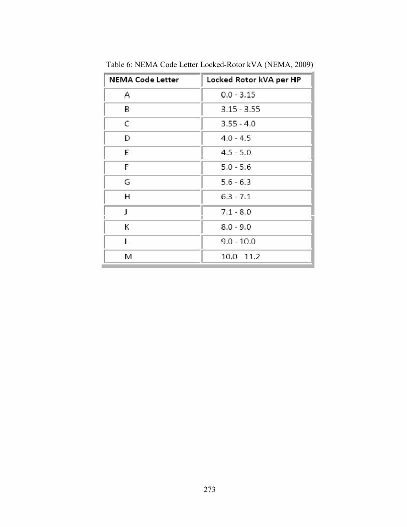
273

Table 6: NEMA Code Letter Locked-Rotor kVA (NEMA, 2009)

274

APPENDIX B

IEEE 34 Node Test Feeder

800

806 808 812 814

810

802 850

818

824 826

816

820

822

828 830 854 856

852

832888 890

838

862

840836860834

842

844

846

848

864

858

275

Overhead Line Configurations (Config.)

Config. Phasing Phase Neutral Spacing ID

ACSR ACSR

300 B A C N 1/0 1/0 500

301 B A C N #2 6/1 #2 6/1 500

302 A N #4 6/1 #4 6/1 510

303 B N #4 6/1 #4 6/1 510

304 B N #2 6/1 #2 6/1 510

Line Segment Data

Node A Node B Length(ft.) Config.

800 802 2580 300

802 806 1730 300

806 808 32230 300

808 810 5804 303

808 812 37500 300

812 814 29730 300

814 850 10 301

816 818 1710 302

816 824 10210 301

818 820 48150 302

820 822 13740 302

824 826 3030 303

824 828 840 301

828 830 20440 301

830 854 520 301

832 858 4900 301

832 888 0 XFM-1

834 860 2020 301

834 842 280 301

836 840 860 301

836 862 280 301

842 844 1350 301

844 846 3640 301

846 848 530 301

850 816 310 301

852 832 10 301

854 856 23330 303

854 852 36830 301

858 864 1620 302

858 834 5830 301

860 836 2680 301

862 838 4860 304

888 890 10560 300

276

Transformer Data

kVA kV-high kV-low R - % X - %

Substation: 2500 69 - D 24.9 -Gr. W 1 8

XFM -1 500 24.9 - Gr.W 4.16 - Gr. W 1.9 4.08

Spot Loads

Node Load Ph-1 Ph-1 Ph-2 Ph-2 Ph-3 Ph-4

Model kW kVAr kW kVAr kW kVAr

860 Y-PQ 20 16 20 16 20 16

840 Y-I 9 7 9 7 9 7

844 Y-Z 135 105 135 105 135 105

848 D-PQ 20 16 20 16 20 16

890 D-I 150 75 150 75 150 75

830 D-Z 10 5 10 5 25 10

Total 344 224 344 224 359 229

Distributed Loads

Node Node Load Ph-1 Ph-1 Ph-2 Ph-2 Ph-3 Ph-3

A B Model kW kVAr kW kVAr kW kVAr

802 806 Y-PQ 0 0 30 15 25 14

808 810 Y-I 0 0 16 8 0 0

818 820 Y-Z 34 17 0 0 0 0

820 822 Y-PQ 135 70 0 0 0 0

816 824 D-I 0 0 5 2 0 0

824 826 Y-I 0 0 40 20 0 0

824 828 Y-PQ 0 0 0 0 4 2

828 830 Y-PQ 7 3 0 0 0 0

854 856 Y-PQ 0 0 4 2 0 0

832 858 D-Z 7 3 2 1 6 3

858 864 Y-PQ 2 1 0 0 0 0

858 834 D-PQ 4 2 15 8 13 7

834 860 D-Z 16 8 20 10 110 55

860 836 D-PQ 30 15 10 6 42 22

836 840 D-I 18 9 22 11 0 0

862 838 Y-PQ 0 0 28 14 0 0

842 844 Y-PQ 9 5 0 0 0 0

844 846 Y-PQ 0 0 25 12 20 11

846 848 Y-PQ 0 0 23 11 0 0

Total 262 133 240 120 220 114

277

Shunt Capacitors

Node Ph-A Ph-B Ph-C

kVAr kVAr kVAr

844 100 100 100

848 150 150 150

Total 250 250 250

Regulator Data

Regulator ID: 1

Line Segment: 814 - 850

Location: 814

Phases: A - B -C

Connection: 3-Ph,LG

Monitoring Phase: A-B-C

Bandwidth: 2.0 volts

PT Ratio: 120

Primary CT Rating: 100

Compensator Settings: Ph-A Ph-B Ph-C

R - Setting: 2.7 2.7 2.7

X - Setting: 1.6 1.6 1.6

Volltage Level: 122 122 122

Regulator ID: 2

Line Segment: 852 - 832

Location: 852

Phases: A - B -C

Connection: 3-Ph,LG

Monitoring Phase: A-B-C

Bandwidth: 2.0 volts

PT Ratio: 120

Primary CT Rating: 100

Compensator Settings: Ph-A Ph-B Ph-C

R - Setting: 2.5 2.5 2.5

X - Setting: 1.5 1.5 1.5

Volltage Level: 124 124 124

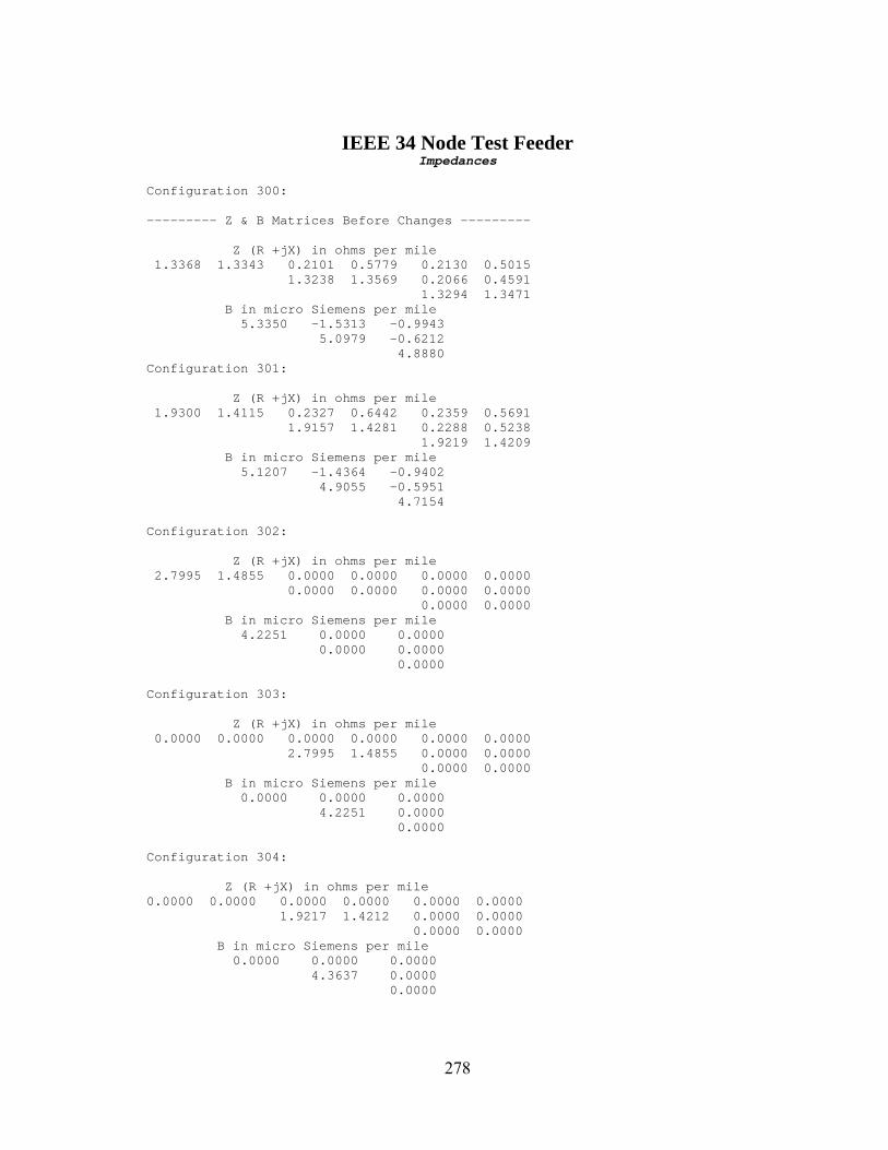
278

IEEE 34 Node Test Feeder Impedances

Configuration 300: --------- Z & B Matrices Before Changes --------- Z (R +jX) in ohms per mile 1.3368 1.3343 0.2101 0.5779 0.2130 0.5015 1.3238 1.3569 0.2066 0.4591 1.3294 1.3471 B in micro Siemens per mile 5.3350 -1.5313 -0.9943 5.0979 -0.6212 4.8880 Configuration 301: Z (R +jX) in ohms per mile 1.9300 1.4115 0.2327 0.6442 0.2359 0.5691 1.9157 1.4281 0.2288 0.5238 1.9219 1.4209 B in micro Siemens per mile 5.1207 -1.4364 -0.9402 4.9055 -0.5951 4.7154 Configuration 302: Z (R +jX) in ohms per mile 2.7995 1.4855 0.0000 0.0000 0.0000 0.0000 0.0000 0.0000 0.0000 0.0000 0.0000 0.0000 B in micro Siemens per mile 4.2251 0.0000 0.0000 0.0000 0.0000 0.0000 Configuration 303: Z (R +jX) in ohms per mile 0.0000 0.0000 0.0000 0.0000 0.0000 0.0000 2.7995 1.4855 0.0000 0.0000 0.0000 0.0000 B in micro Siemens per mile 0.0000 0.0000 0.0000 4.2251 0.0000 0.0000 Configuration 304: Z (R +jX) in ohms per mile 0.0000 0.0000 0.0000 0.0000 0.0000 0.0000 1.9217 1.4212 0.0000 0.0000 0.0000 0.0000 B in micro Siemens per mile 0.0000 0.0000 0.0000 4.3637 0.0000 0.0000

279

Power Flow Results - R A D I A L F L O W S U M M A R Y - DATE: 6-24-2004 AT 16:34:11 HOURS --- SUBSTATION: IEEE 34; FEEDER: IEEE 34 ------------------------------------------------------------------------------- SYSTEM PHASE PHASE PHASE TOTAL INPUT -------(A)-------|-------(B)-------|-------(C)-------|------------------ kW : 759.136 | 666.663 | 617.072 | 2042.872 kVAr : 171.727 | 90.137 | 28.394 | 290.258 kVA : 778.318 | 672.729 | 617.725 | 2063.389 PF : .9754 | .9910 | .9989 | .9901 LOAD --(A-N)----(A-B)-|--(B-N)----(B-C)-|--(C-N)----(C-A)-|---WYE-----DELTA-- kW : 359.9 246.4| 339.3 243.3| 221.8 359.0| 921.0 848.8 TOT : 606.322 | 582.662 | 580.840 | 1769.824 | | | kVAr : 230.9 128.7| 216.9 128.7| 161.8 184.6| 609.6 441.9 TOT : 359.531 | 345.609 | 346.407 | 1051.547 | | | kVA : 427.6 278.0| 402.7 275.3| 274.6 403.7| 1104.5 957.0 TOT : 704.903 | 677.452 | 676.293 | 2058.647 | | | PF : .8417 .8864| .8425 .8840| .8078 .8894| .8339 .8870 TOT : .8601 | .8601 | .8589 | .8597 LOSSES ------(A)-------|-------(B)-------|-------(C)-------|------------------ kW : 114.836 | 80.389 | 77.824 | 273.049 kVAr : 14.200 | 10.989 | 9.810 | 34.999 kVA : 115.711 | 81.137 | 78.440 | 275.283 CAPAC --(A-N)----(A-B)-|--(B-N)----(B-C)-|--(C-N)----(C-A)-|---WYE-----DELTA-- R-kVA: 250.0 .0| 250.0 .0| 250.0 .0| 750.0 .0 TOT : 250.000 | 250.000 | 250.000 | 750.000 | | | A-kVA: 265.7 .0| 264.8 .0| 265.9 .0| 796.3 .0 TOT : 265.658 | 264.760 | 265.869 | 796.287

280

--- V O L T A G E P R O F I L E ---- DATE: 6-24-2004 AT 16:34:18 HOURS ---- SUBSTATION: IEEE 34; FEEDER: IEEE 34 ------------------------------------------------------------------------------- NODE | MAG ANGLE | MAG ANGLE | MAG ANGLE |mi.to SR ------------------------------------------------------------------------------- ______|_______ A-N ______ |_______ B-N _______ |_______ C-N _______ | 800 | 1.0500 at .00 | 1.0500 at -120.00 | 1.0500 at 120.00 | .000 802 | 1.0475 at -.05 | 1.0484 at -120.07 | 1.0484 at 119.95 | .489 806 | 1.0457 at -.08 | 1.0474 at -120.11 | 1.0474 at 119.92 | .816 808 | 1.0136 at -.75 | 1.0296 at -120.95 | 1.0289 at 119.30 | 6.920 810 | | 1.0294 at -120.95 | | 8.020 812 | .9763 at -1.57 | 1.0100 at -121.92 | 1.0069 at 118.59 | 14.023 814 | .9467 at -2.26 | .9945 at -122.70 | .9893 at 118.01 | 19.653 RG10 | 1.0177 at -2.26 | 1.0255 at -122.70 | 1.0203 at 118.01 | 19.654 850 | 1.0176 at -2.26 | 1.0255 at -122.70 | 1.0203 at 118.01 | 19.655 816 | 1.0172 at -2.26 | 1.0253 at -122.71 | 1.0200 at 118.01 | 19.714 818 | 1.0163 at -2.27 | | | 20.038 820 | .9926 at -2.32 | | | 29.157 822 | .9895 at -2.33 | | | 31.760 824 | 1.0082 at -2.37 | 1.0158 at -122.94 | 1.0116 at 117.76 | 21.648 826 | | 1.0156 at -122.94 | | 22.222 828 | 1.0074 at -2.38 | 1.0151 at -122.95 | 1.0109 at 117.75 | 21.807 830 | .9894 at -2.63 | .9982 at -123.39 | .9938 at 117.25 | 25.678 854 | .9890 at -2.64 | .9978 at -123.40 | .9934 at 117.24 | 25.777 852 | .9581 at -3.11 | .9680 at -124.18 | .9637 at 116.33 | 32.752 RG11 | 1.0359 at -3.11 | 1.0345 at -124.18 | 1.0360 at 116.33 | 32.752 832 | 1.0359 at -3.11 | 1.0345 at -124.18 | 1.0360 at 116.33 | 32.754 858 | 1.0336 at -3.17 | 1.0322 at -124.28 | 1.0338 at 116.22 | 33.682 834 | 1.0309 at -3.24 | 1.0295 at -124.39 | 1.0313 at 116.09 | 34.786 842 | 1.0309 at -3.25 | 1.0294 at -124.39 | 1.0313 at 116.09 | 34.839 844 | 1.0307 at -3.27 | 1.0291 at -124.42 | 1.0311 at 116.06 | 35.095 846 | 1.0309 at -3.32 | 1.0291 at -124.46 | 1.0313 at 116.01 | 35.784 848 | 1.0310 at -3.32 | 1.0291 at -124.47 | 1.0314 at 116.00 | 35.885 860 | 1.0305 at -3.24 | 1.0291 at -124.39 | 1.0310 at 116.09 | 35.169 836 | 1.0303 at -3.23 | 1.0287 at -124.39 | 1.0308 at 116.09 | 35.677 840 | 1.0303 at -3.23 | 1.0287 at -124.39 | 1.0308 at 116.09 | 35.839 862 | 1.0303 at -3.23 | 1.0287 at -124.39 | 1.0308 at 116.09 | 35.730 838 | | 1.0285 at -124.39 | | 36.650 864 | 1.0336 at -3.17 | | | 33.989 XF10 | .9997 at -4.63 | .9983 at -125.73 | 1.0000 at 114.82 | 32.754 888 | .9996 at -4.64 | .9983 at -125.73 | 1.0000 at 114.82 | 32.754 890 | .9167 at -5.19 | .9235 at -126.78 | .9177 at 113.98 | 34.754 856 | | .9977 at -123.41 | | 30.195 ----------- VOLTAGE REGULATOR DATA ---- DATE: 6-24-2004 AT 16:34:22 HOURS -- SUBSTATION: IEEE 34; FEEDER: IEEE 34 _______________________________________________________________________________ [NODE]--[VREG]-----[SEG]------[NODE] MODEL OPT BNDW 814 RG10 850 850 Phase A & B & C, Wye RX 2.00 ........................................................................ PHASE LDCTR VOLT HOLD R-VOLT X-VOLT PT RATIO CT RATE TAP 1 122.000 2.700 1.600 120.00 100.00 12 2 122.000 2.700 1.600 120.00 100.00 5 3 122.000 2.700 1.600 120.00 100.00 5 _______________________________________________________________________________ [NODE]--[VREG]-----[SEG]------[NODE] MODEL OPT BNDW 852 RG11 832 832 Phase A & B & C, Wye RX 2.00 ........................................................................ PHASE LDCTR VOLT HOLD R-VOLT X-VOLT PT RATIO CT RATE TAP 1 124.000 2.500 1.500 120.00 100.00 13 2 124.000 2.500 1.500 120.00 100.00 11 3 124.000 2.500 1.500 120.00 100.00 12

281

- R A D I A L P O W E R F L O W --- DATE: 6-24-2004 AT 16:34:32 HOURS --- SUBSTATION: IEEE 34; FEEDER: IEEE 34 ------------------------------------------------------------------------------- NODE VALUE PHASE A PHASE B PHASE C UNT O/L< (LINE A) (LINE B) (LINE C) 60.% ---------------------*--------A-------*-------B-------*-------C-------*-------- NODE: 800 VOLTS: 1.050 .00 1.050 -120.00 1.050 120.00 MAG/ANG kVll 24.900 NO LOAD OR CAPACITOR REPRESENTED AT SOURCE NODE TO NODE 802 .......: 51.56 -12.74 44.57 -127.70 40.92 117.37 AMP/DG <802 > LOSS= 3.472: ( 1.637) ( .978) ( .858) kW ---------------------*--------A-------*-------B-------*-------C-------*-------- NODE: 802 VOLTS: 1.047 -.05 1.048 -120.07 1.048 119.95 MAG/ANG -LD: .00 .00 .00 .00 .00 .00 kW/kVR kVll 24.900 CAP: .00 .00 .00 kVR FROM NODE 800 .....: 51.58 -12.80 44.57 -127.76 40.93 117.31 AMP/DG <802 > LOSS= 3.472: ( 1.637) ( .978) ( .858) kW TO NODE 806 .......: 51.58 -12.80 44.57 -127.76 40.93 117.31 AMP/DG <806 > LOSS= 2.272: ( 1.102) ( .618) ( .552) kW ---------------------*--------A-------*-------B-------*-------C-------*-------- NODE: 806 VOLTS: 1.046 -.08 1.047 -120.11 1.047 119.92 MAG/ANG -LD: .00 .00 .00 .00 .00 .00 kW/kVR kVll 24.900 CAP: .00 .00 .00 kVR FROM NODE 802 .....: 51.59 -12.83 42.47 -126.83 39.24 118.52 AMP/DG <806 > LOSS= 2.272: ( 1.102) ( .618) ( .552) kW TO NODE 808 .......: 51.59 -12.83 42.47 -126.83 39.24 118.52 AMP/DG <808 > LOSS= 41.339: ( 20.677) ( 10.780) ( 9.882) kW ---------------------*--------A-------*-------B-------*-------C-------*-------- NODE: 808 VOLTS: 1.014 -.75 1.030 -120.95 1.029 119.30 MAG/ANG -LD: .00 .00 .00 .00 .00 .00 kW/kVR kVll 24.900 CAP: .00 .00 .00 kVR FROM NODE 806 .....: 51.76 -13.47 42.46 -127.59 39.28 117.76 AMP/DG <808 > LOSS= 41.339: ( 20.677) ( 10.780) ( 9.882) kW TO NODE 810 .......: 1.22 -144.62 AMP/DG <810 > LOSS= .002: ( .002) kW TO NODE 812 .......: 51.76 -13.47 41.30 -127.10 39.28 117.76 AMP/DG <812 > LOSS= 47.531: ( 24.126) ( 11.644) ( 11.761) kW ---------------------*--------A-------*-------B-------*-------C-------*-------- NODE: 810 VOLTS: 1.029 -120.95 MAG/ANG -LD: .00 .00 kW/kVR kVll 24.900 CAP: .00 kVR FROM NODE 808 .....: .00 .00 AMP/DG <810 > LOSS= .002: ( .002) kW

282

- R A D I A L P O W E R F L O W --- DATE: 6-24-2004 AT 16:34:32 HOURS --- SUBSTATION: IEEE 34; FEEDER: IEEE 34 ------------------------------------------------------------------------------- NODE VALUE PHASE A PHASE B PHASE C UNT O/L< (LINE A) (LINE B) (LINE C) 60.% ---------------------*--------A-------*-------B-------*-------C-------*-------- NODE: 812 VOLTS: .976 -1.57 1.010 -121.92 1.007 118.59 MAG/ANG -LD: .00 .00 .00 .00 .00 .00 kW/kVR kVll 24.900 CAP: .00 .00 .00 kVR FROM NODE 808 .....: 51.95 -14.18 41.29 -127.99 39.33 116.90 AMP/DG <812 > LOSS= 47.531: ( 24.126) ( 11.644) ( 11.761) kW TO NODE 814 .......: 51.95 -14.18 41.29 -127.99 39.33 116.90 AMP/DG <814 > LOSS= 37.790: ( 19.245) ( 9.140) ( 9.404) kW ---------------------*--------A-------*-------B-------*-------C-------*-------- NODE: 814 VOLTS: .947 -2.26 .994 -122.70 .989 118.01 MAG/ANG -LD: .00 .00 .00 .00 .00 .00 kW/kVR kVll 24.900 CAP: .00 .00 .00 kVR FROM NODE 812 .....: 52.10 -14.73 41.29 -128.69 39.37 116.23 AMP/DG <814 > LOSS= 37.790: ( 19.245) ( 9.140) ( 9.404) kW TO NODE RG10 .<VRG>.: 52.10 -14.73 41.29 -128.69 39.37 116.23 AMP/DG <RG10 > LOSS= .000: ( .000) ( .000) ( .000) kW ---------------------*--------A-------*-------B-------*-------C-------*-------- NODE: RG10 VOLTS: 1.018 -2.26 1.026 -122.70 1.020 118.01 MAG/ANG -LD: .00 .00 .00 .00 .00 .00 kW/kVR kVll 24.900 CAP: .00 .00 .00 kVR FROM NODE 814 <VRG>: 48.47 -14.73 40.04 -128.69 38.17 116.23 AMP/DG <RG10 > LOSS= .000: ( .000) ( .000) ( .000) kW TO NODE 850 .......: 48.47 -14.73 40.04 -128.69 38.17 116.23 AMP/DG <850 > LOSS= .017: ( .008) ( .005) ( .005) kW ---------------------*--------A-------*-------B-------*-------C-------*-------- NODE: 850 VOLTS: 1.018 -2.26 1.026 -122.70 1.020 118.01 MAG/ANG -LD: .00 .00 .00 .00 .00 .00 kW/kVR kVll 24.900 CAP: .00 .00 .00 kVR FROM NODE RG10 .....: 48.47 -14.73 40.04 -128.69 38.17 116.23 AMP/DG <850 > LOSS= .017: ( .008) ( .005) ( .005) kW TO NODE 816 .......: 48.47 -14.73 40.04 -128.69 38.17 116.23 AMP/DG <816 > LOSS= .538: ( .254) ( .145) ( .139) kW ---------------------*--------A-------*-------B-------*-------C-------*-------- NODE: 816 VOLTS: 1.017 -2.26 1.025 -122.71 1.020 118.01 MAG/ANG -LD: .00 .00 .00 .00 .00 .00 kW/kVR kVll 24.900 CAP: .00 .00 .00 kVR FROM NODE 850 .....: 48.47 -14.74 40.04 -128.70 38.17 116.23 AMP/DG <816 > LOSS= .538: ( .254) ( .145) ( .139) kW TO NODE 818 .......: 13.02 -26.69 AMP/DG <818 > LOSS= .154: ( .154) kW TO NODE 824 .......: 35.83 -10.42 40.04 -128.70 38.17 116.23 AMP/DG <824 > LOSS= 14.181: ( 4.312) ( 5.444) ( 4.425) kW

283

- R A D I A L P O W E R F L O W --- DATE: 6-24-2004 AT 16:34:32 HOURS --- SUBSTATION: IEEE 34; FEEDER: IEEE 34 ------------------------------------------------------------------------------- NODE VALUE PHASE A PHASE B PHASE C UNT O/L< (LINE A) (LINE B) (LINE C) 60.% ---------------------*--------A-------*-------B-------*-------C-------*-------- NODE: 818 VOLTS: 1.016 -2.27 MAG/ANG -LD: .00 .00 kW/kVR kVll 24.900 CAP: .00 kVR FROM NODE 816 .....: 13.03 -26.77 AMP/DG <818 > LOSS= .154: ( .154) kW TO NODE 820 .......: 13.03 -26.77 AMP/DG <820 > LOSS= 3.614: ( 3.614) kW ---------------------*--------A-------*-------B-------*-------C-------*-------- NODE: 820 VOLTS: .993 -2.32 MAG/ANG -LD: .00 .00 kW/kVR kVll 24.900 CAP: .00 kVR FROM NODE 818 .....: 10.62 -28.98 AMP/DG <820 > LOSS= 3.614: ( 3.614) kW TO NODE 822 .......: 10.62 -28.98 AMP/DG <822 > LOSS= .413: ( .413) kW ---------------------*--------A-------*-------B-------*-------C-------*-------- NODE: 822 VOLTS: .990 -2.33 MAG/ANG -LD: .00 .00 kW/kVR kVll 24.900 CAP: .00 kVR FROM NODE 820 .....: .00 .00 AMP/DG <822 > LOSS= .413: ( .413) kW ---------------------*--------A-------*-------B-------*-------C-------*-------- NODE: 824 VOLTS: 1.008 -2.37 1.016 -122.94 1.012 117.76 MAG/ANG -LD: .00 .00 .00 .00 .00 .00 kW/kVR kVll 24.900 CAP: .00 .00 .00 kVR FROM NODE 816 .....: 35.87 -10.70 39.82 -129.02 38.05 116.25 AMP/DG <824 > LOSS= 14.181: ( 4.312) ( 5.444) ( 4.425) kW TO NODE 826 .......: 3.10 -148.92 AMP/DG <826 > LOSS= .008: ( .008) kW TO NODE 828 .......: 35.87 -10.70 36.93 -127.39 38.05 116.25 AMP/DG <828 > LOSS= 1.108: ( .361) ( .393) ( .354) kW ---------------------*--------A-------*-------B-------*-------C-------*-------- NODE: 826 VOLTS: 1.016 -122.94 MAG/ANG -LD: .00 .00 kW/kVR kVll 24.900 CAP: .00 kVR FROM NODE 824 .....: .00 .00 AMP/DG <826 > LOSS= .008: ( .008) kW

284

- R A D I A L P O W E R F L O W --- DATE: 6-24-2004 AT 16:34:32 HOURS --- SUBSTATION: IEEE 34; FEEDER: IEEE 34 ------------------------------------------------------------------------------- NODE VALUE PHASE A PHASE B PHASE C UNT O/L< (LINE A) (LINE B) (LINE C) 60.% ---------------------*--------A-------*-------B-------*-------C-------*-------- NODE: 828 VOLTS: 1.007 -2.38 1.015 -122.95 1.011 117.75 MAG/ANG -LD: .00 .00 .00 .00 .00 .00 kW/kVR kVll 24.900 CAP: .00 .00 .00 kVR FROM NODE 824 .....: 35.87 -10.72 36.93 -127.41 37.77 116.42 AMP/DG <828 > LOSS= 1.108: ( .361) ( .393) ( .354) kW TO NODE 830 .......: 35.87 -10.72 36.93 -127.41 37.77 116.42 AMP/DG <830 > LOSS= 26.587: ( 8.443) ( 9.214) ( 8.930) kW ---------------------*--------A-------*-------B-------*-------C-------*-------- NODE: 830 VOLTS: .989 -2.63 .998 -123.39 .994 117.25 MAG/ANG D-LD: 9.95 4.98 9.86 4.93 24.55 9.82 kW/kVR kVll 24.900 Y CAP: .00 .00 .00 kVR FROM NODE 828 .....: 35.43 -11.06 36.91 -127.92 37.79 115.96 AMP/DG <830 > LOSS= 26.587: ( 8.443) ( 9.214) ( 8.930) kW TO NODE 854 .......: 34.22 -9.97 36.19 -127.47 36.49 116.26 AMP/DG <854 > LOSS= .635: ( .197) ( .227) ( .211) kW ---------------------*--------A-------*-------B-------*-------C-------*-------- NODE: 854 VOLTS: .989 -2.64 .998 -123.40 .993 117.24 MAG/ANG -LD: .00 .00 .00 .00 .00 .00 kW/kVR kVll 24.900 CAP: .00 .00 .00 kVR FROM NODE 830 .....: 34.23 -9.99 36.19 -127.48 36.49 116.25 AMP/DG <854 > LOSS= .635: ( .197) ( .227) ( .211) kW TO NODE 852 .......: 34.23 -9.99 35.93 -127.72 36.49 116.25 AMP/DG <852 > LOSS= 44.798: ( 13.996) ( 15.778) ( 15.023) kW TO NODE 856 .......: .31 -98.70 AMP/DG <856 > LOSS= .001: ( .001) kW ---------------------*--------A-------*-------B-------*-------C-------*-------- NODE: 852 VOLTS: .958 -3.11 .968 -124.18 .964 116.33 MAG/ANG -LD: .00 .00 .00 .00 .00 .00 kW/kVR kVll 24.900 CAP: .00 .00 .00 kVR FROM NODE 854 .....: 34.35 -11.00 35.90 -128.66 36.52 115.41 AMP/DG <852 > LOSS= 44.798: ( 13.996) ( 15.778) ( 15.023) kW TO NODE RG11 .<VRG>.: 34.35 -11.00 35.90 -128.66 36.52 115.41 AMP/DG <RG11 > LOSS= .000: ( .000) ( .000) ( .000) kW ---------------------*--------A-------*-------B-------*-------C-------*-------- NODE: RG11 VOLTS: 1.036 -3.11 1.035 -124.18 1.036 116.33 MAG/ANG -LD: .00 .00 .00 .00 .00 .00 kW/kVR kVll 24.900 CAP: .00 .00 .00 kVR FROM NODE 852 <VRG>: 31.77 -11.00 33.59 -128.66 33.98 115.41 AMP/DG <RG11 > LOSS= .000: ( .000) ( .000) ( .000) kW TO NODE 832 .......: 31.77 -11.00 33.59 -128.66 33.98 115.41 AMP/DG <832 > LOSS= .011: ( .003) ( .004) ( .004) kW

285

- R A D I A L P O W E R F L O W --- DATE: 6-24-2004 AT 16:34:32 HOURS --- SUBSTATION: IEEE 34; FEEDER: IEEE 34 ------------------------------------------------------------------------------- NODE VALUE PHASE A PHASE B PHASE C UNT O/L< (LINE A) (LINE B) (LINE C) 60.% ---------------------*--------A-------*-------B-------*-------C-------*-------- NODE: 832 VOLTS: 1.036 -3.11 1.035 -124.18 1.036 116.33 MAG/ANG -LD: .00 .00 .00 .00 .00 .00 kW/kVR kVll 24.900 CAP: .00 .00 .00 kVR FROM NODE RG11 .....: 31.77 -11.00 33.59 -128.66 33.98 115.41 AMP/DG <832 > LOSS= .011: ( .003) ( .004) ( .004) kW TO NODE 858 .......: 21.31 .47 23.40 -116.89 24.34 128.36 AMP/DG <858 > LOSS= 2.467: ( .643) ( .997) ( .827) kW TO NODE XF10 .......: 11.68 -32.29 11.70 -152.73 11.61 87.39 AMP/DG < <XF10 > LOSS= 9.625: ( 3.196) ( 3.241) ( 3.187) kW ---------------------*--------A-------*-------B-------*-------C-------*-------- NODE: 858 VOLTS: 1.034 -3.17 1.032 -124.28 1.034 116.22 MAG/ANG -LD: .00 .00 .00 .00 .00 .00 kW/kVR kVll 24.900 CAP: .00 .00 .00 kVR FROM NODE 832 .....: 20.86 .86 23.13 -116.39 24.02 128.48 AMP/DG <858 > LOSS= 2.467: ( .643) ( .997) ( .827) kW TO NODE 834 .......: 20.73 1.01 23.13 -116.39 24.02 128.48 AMP/DG <834 > LOSS= 2.798: ( .717) ( 1.145) ( .936) kW TO NODE 864 .......: .14 -22.82 AMP/DG <864 > LOSS= .000: ( .000) kW ---------------------*--------A-------*-------B-------*-------C-------*-------- NODE: 834 VOLTS: 1.031 -3.24 1.029 -124.39 1.031 116.09 MAG/ANG -LD: .00 .00 .00 .00 .00 .00 kW/kVR kVll 24.900 CAP: .00 .00 .00 kVR FROM NODE 858 .....: 20.29 2.18 22.37 -116.07 23.23 130.06 AMP/DG <834 > LOSS= 2.798: ( .717) ( 1.145) ( .936) kW TO NODE 842 .......: 14.75 34.68 16.30 -95.63 15.12 151.05 AMP/DG <842 > LOSS= .064: ( .015) ( .032) ( .017) kW TO NODE 860 .......: 11.16 -43.05 9.09 -154.82 10.60 99.34 AMP/DG <860 > LOSS= .141: ( .021) ( .104) ( .017) kW ---------------------*--------A-------*-------B-------*-------C-------*-------- NODE: 842 VOLTS: 1.031 -3.25 1.029 -124.39 1.031 116.09 MAG/ANG -LD: .00 .00 .00 .00 .00 .00 kW/kVR kVll 24.900 CAP: .00 .00 .00 kVR FROM NODE 834 .....: 14.74 34.67 16.30 -95.64 15.12 151.03 AMP/DG <842 > LOSS= .064: ( .015) ( .032) ( .017) kW TO NODE 844 .......: 14.74 34.67 16.30 -95.64 15.12 151.03 AMP/DG <844 > LOSS= .306: ( .068) ( .156) ( .083) kW

286

- R A D I A L P O W E R F L O W --- DATE: 6-24-2004 AT 16:34:32 HOURS --- SUBSTATION: IEEE 34; FEEDER: IEEE 34 ------------------------------------------------------------------------------- NODE VALUE PHASE A PHASE B PHASE C UNT O/L< (LINE A) (LINE B) (LINE C) 60.% ---------------------*--------A-------*-------B-------*-------C-------*-------- NODE: 844 VOLTS: 1.031 -3.27 1.029 -124.42 1.031 116.06 MAG/ANG Y-LD: 143.41 111.54 142.97 111.20 143.51 111.62 kW/kVR kVll 24.900 Y CAP: 106.23 105.90 106.31 kVR FROM NODE 842 .....: 14.47 37.12 16.29 -95.71 15.11 150.97 AMP/DG <844 > LOSS= .306: ( .068) ( .156) ( .083) kW TO NODE 846 .......: 9.83 78.88 9.40 -63.87 9.40 -170.67 AMP/DG <846 > LOSS= .323: ( .043) ( .212) ( .068) kW ---------------------*--------A-------*-------B-------*-------C-------*-------- NODE: 846 VOLTS: 1.031 -3.32 1.029 -124.46 1.031 116.01 MAG/ANG -LD: .00 .00 .00 .00 .00 .00 kW/kVR kVll 24.900 CAP: .00 .00 .00 kVR FROM NODE 844 .....: 9.76 78.80 9.40 -52.54 9.78 -161.93 AMP/DG <846 > LOSS= .323: ( .043) ( .212) ( .068) kW TO NODE 848 .......: 9.76 78.80 9.40 -52.54 9.78 -161.93 AMP/DG <848 > LOSS= .048: ( .007) ( .031) ( .010) kW ---------------------*--------A-------*-------B-------*-------C-------*-------- NODE: 848 VOLTS: 1.031 -3.32 1.029 -124.47 1.031 116.00 MAG/ANG D-LD: 20.00 16.00 20.00 16.00 20.00 16.00 kW/kVR kVll 24.900 Y CAP: 159.43 158.86 159.56 kVR FROM NODE 846 .....: 9.76 78.79 9.77 -42.47 9.78 -161.94 AMP/DG <848 > LOSS= .048: ( .007) ( .031) ( .010) kW ---------------------*--------A-------*-------B-------*-------C-------*-------- NODE: 860 VOLTS: 1.030 -3.24 1.029 -124.39 1.031 116.09 MAG/ANG Y-LD: 20.00 16.00 20.00 16.00 20.00 16.00 kW/kVR kVll 24.900 Y CAP: .00 .00 .00 kVR FROM NODE 834 .....: 5.87 -33.62 7.68 -156.52 5.29 86.10 AMP/DG <860 > LOSS= .141: ( .021) ( .104) ( .017) kW TO NODE 836 .......: 4.16 -30.19 5.96 -154.63 3.60 90.25 AMP/DG <836 > LOSS= .039: ( -.035) ( .103) ( -.028) kW ---------------------*--------A-------*-------B-------*-------C-------*-------- NODE: 836 VOLTS: 1.030 -3.23 1.029 -124.39 1.031 116.09 MAG/ANG -LD: .00 .00 .00 .00 .00 .00 kW/kVR kVll 24.900 CAP: .00 .00 .00 kVR FROM NODE 860 .....: 1.49 -19.83 4.42 -150.74 1.74 68.08 AMP/DG <836 > LOSS= .039: ( -.035) ( .103) ( -.028) kW TO NODE 840 .......: 1.50 -20.01 2.33 -151.97 1.75 68.00 AMP/DG <840 > LOSS= .002: ( -.014) ( .026) ( -.010) kW TO NODE 862 .......: .00 .00 2.09 -149.38 .00 .00 AMP/DG <862 > LOSS= .000: ( -.005) ( .009) ( -.004) kW

287

- R A D I A L P O W E R F L O W --- DATE: 6-24-2004 AT 16:34:32 HOURS --- SUBSTATION: IEEE 34; FEEDER: IEEE 34 ------------------------------------------------------------------------------- NODE VALUE PHASE A PHASE B PHASE C UNT O/L< (LINE A) (LINE B) (LINE C) 60.% ---------------------*--------A-------*-------B-------*-------C-------*-------- NODE: 840 VOLTS: 1.030 -3.23 1.029 -124.39 1.031 116.09 MAG/ANG Y-LD: 9.27 7.21 9.26 7.20 9.28 7.22 kW/kVR kVll 24.900 Y CAP: .00 .00 .00 kVR FROM NODE 836 .....: .79 -41.11 .79 -162.26 .79 78.21 AMP/DG <840 > LOSS= .002: ( -.014) ( .026) ( -.010) kW ---------------------*--------A-------*-------B-------*-------C-------*-------- NODE: 862 VOLTS: 1.030 -3.23 1.029 -124.39 1.031 116.09 MAG/ANG -LD: .00 .00 .00 .00 .00 .00 kW/kVR kVll 24.900 CAP: .00 .00 .00 kVR FROM NODE 836 .....: .00 .00 2.09 -149.50 .00 .00 AMP/DG <862 > LOSS= .000: ( -.005) ( .009) ( -.004) kW TO NODE 838 .......: 2.09 -149.50 AMP/DG <838 > LOSS= .004: ( .004) kW ---------------------*--------A-------*-------B-------*-------C-------*-------- NODE: 838 VOLTS: 1.029 -124.39 MAG/ANG -LD: .00 .00 kW/kVR kVll 24.900 CAP: .00 kVR FROM NODE 862 .....: .00 .00 AMP/DG <838 > LOSS= .004: ( .004) kW ---------------------*--------A-------*-------B-------*-------C-------*-------- NODE: 864 VOLTS: 1.034 -3.17 MAG/ANG -LD: .00 .00 kW/kVR kVll 24.900 CAP: .00 kVR FROM NODE 858 .....: .00 .00 AMP/DG <864 > LOSS= .000: ( .000) kW ---------------------*--------A-------*-------B-------*-------C-------*-------- NODE: XF10 VOLTS: 1.000 -4.63 .998 -125.73 1.000 114.82 MAG/ANG -LD: .00 .00 .00 .00 .00 .00 kW/kVR kVll 4.160 CAP: .00 .00 .00 kVR FROM NODE 832 .....: 69.90 -32.29 70.04 -152.73 69.50 87.39 AMP/DG < <XF10 > LOSS= 9.625: ( 3.196) ( 3.241) ( 3.187) kW TO NODE 888 .......: 69.90 -32.29 70.04 -152.73 69.50 87.39 AMP/DG <888 > LOSS= .000: ( .000) ( .000) ( .000) kW ---------------------*--------A-------*-------B-------*-------C-------*-------- NODE: 888 VOLTS: 1.000 -4.64 .998 -125.73 1.000 114.82 MAG/ANG -LD: .00 .00 .00 .00 .00 .00 kW/kVR kVll 4.160 CAP: .00 .00 .00 kVR FROM NODE XF10 .....: 69.90 -32.29 70.04 -152.73 69.50 87.39 AMP/DG <888 > LOSS= .000: ( .000) ( .000) ( .000) kW TO NODE 890 .......: 69.90 -32.29 70.04 -152.73 69.50 87.39 AMP/DG <890 > LOSS= 32.760: ( 11.638) ( 9.950) ( 11.173) kW

288

- R A D I A L P O W E R F L O W --- DATE: 6-24-2004 AT 16:34:32 HOURS --- SUBSTATION: IEEE 34; FEEDER: IEEE 34 ------------------------------------------------------------------------------- NODE VALUE PHASE A PHASE B PHASE C UNT O/L< (LINE A) (LINE B) (LINE C) 60.% ---------------------*--------A-------*-------B-------*-------C-------*-------- NODE: 890 VOLTS: .917 -5.19 .924 -126.78 .918 113.98 MAG/ANG D-LD: 139.11 69.55 137.56 68.78 137.01 68.50 kW/kVR kVll 4.160 Y CAP: .00 .00 .00 kVR FROM NODE 888 .....: 69.91 -32.31 70.05 -152.75 69.51 87.37 AMP/DG <890 > LOSS= 32.760: ( 11.638) ( 9.950) ( 11.173) kW ---------------------*--------A-------*-------B-------*-------C-------*-------- NODE: 856 VOLTS: .998 -123.41 MAG/ANG -LD: .00 .00 kW/kVR kVll 24.900 CAP: .00 kVR FROM NODE 854 .....: .00 .00 AMP/DG <856 > LOSS= .001: ( .001) kW

dynamic reactive power control of isolated power … · 2017-04-28 · this dissertation presents...

Documents