dynamic response of high-rise building structures to blast loading
TRANSCRIPT

Dynamic response of high-rise building structures
to blast loading
L. J. van der Meer (0520033)
Graduation committee: Dr ir M. C. M. Bakker
Prof dr ir J. G. M. Kerstens Dr ir J. Weerheijm
Research report: A-2008.3, O-2008.8
April 2008


i
Acknowledgements
First of all I would like to thank my graduation committee for their guidance, suggestionsand advice:
• Dr ir Monique Bakker, Eindhoven University of Technology
• Prof dr ir Jan Kerstens, Eindhoven University of Technology
• Dr ir Jaap Weerheijm, Delft University of Technology, TNO
Furthermore I am very thankful to David Rijlaarsdam, Mechanical Engineering student inthe direction of Dynamics and Control, for his help with Matlab and the discussions we hadregarding the contents of this graduation project. I would also like to express gratitude toHenk van Harn of Adams Bouwadvies, for the opportunity to gather information about the LaFenetre building in the Hague, although the building structure turned out to be to complexto function as an example in this report.
L. J. van der Meer

ii
Summary
In the Netherlands, the railway line from the harbor in Rotterdam to the Ruhr area inGermany is used for the transport of many hazardous substances. One of the risks involved isthat of a BLEVE from a vessel containing a liquified gas such as LPG. A BLEVE is a boilingliquid expanding vapor explosion, which is a result of the catastrophic failure of the vessel,a sudden decompression and explosive evaporation of the liquified gas. One of the hazardsassociated with a BLEVE is a shock wave, the BLEVE blast. Buildings in the neighborhoodof the railway line have a certain risk of being struck by this extreme type of loading. Indensely built areas such as Tilburg, residential and office buildings are within a range of 20mof the railway line.
Dutch guidelines use empirical data from the Second World War to estimate damageof buildings up to four stories due to blast loads. For higher buildings, a single degree offreedom (SDOF) approach is proposed. Other literature also focusses on SDOF response,which means that the building is assumed to vibrate with a single shape at the first naturalfrequency. This graduation project was used to evaluate the continuous response of high-rise building structures to blast loading in general and BLEVE blast loading in particular.Continuous response is an infinite sum of mode shapes vibrating at their natural frequencies.
To obtain dynamic response of buildings to blast loading, a blast load and impulse distri-bution on a facade needs to be established first. Blast parameters are available in literatureversus range and charge mass for high explosives. The relations between the various blastparameters are based on gas dynamics and also apply to BLEVEs, except for duration andimpulse which are underestimated. More recent literature is available to determine BLEVEoverpressure and duration versus range and liquid mass. Impulse can be derived from over-pressure and duration. Other blast parameters can be derived from overpressure. Hence, ablast load and impulse distribution on a facade can be determined.
The second requirement for the determination of dynamic response is an appropriatedynamic model of the building structure. For SDOF response, an equivalent SDOF system isobtained. For continuous response, a stability element is modeled as an equivalent continuousbeam. Special attention is given to assumptions, which are done during the modeling process.
The SDOF response is determined analytically for linear-elastic material behavior, ideal-ized blast loads and without damping. The response is divided in three regimes: impulsive,dynamic and quasi-static. The response regime is determined by the ratio of the durationof the blast load on the building and the natural period of vibration of the building. Themaximum response in the different regimes is given in response diagrams, such as the pressure-impulse diagram, which gives a damage envelope for a certain degree of damage or failurecriterium. For a SDOF system which represents a building, internal forces are proportional tothe top displacement, which is chosen as the degree of freedom. Therefore, all failure criteriacan be linked to a critical top displacement.
Dynamic response of high-rise building structures to blast loading

iii
The continuous response is determined by analysis of a continuous Timoshenko beam,representing a building. The Timoshenko beam includes deflection due to bending, shear androtation of the cross section. Modal contribution factors for base moment and base shear arederived, which give the contribution of a mode as a percentage of the total response. Themodal response can be analyzed as a SDOF system. The total response is a sum of the modalresponses multiplied by the modal contribution factors. Often a few modes are enough forsufficient accuracy. A method is given to approximate the overall maximum of the continuousresponse. The failure criterium is directly linked to base shear or base moment response.
Upon comparison of SDOF and continuous response, it is concluded that the SDOF systemis not conservative for response in the impulsive regime, whereas the quasi-static response issimilar for both models. BLEVE blast loading on high-rise buildings is likely in the impulsiveregime. It can be concluded that response of high-rise buildings to loads in the impulsiveregime, among which BLEVE blast, can not be analyzed with a SDOF system.
These conclusions are based on overall response. It is assumed that the building facade isable to transfer all loading to the bearing structure. The influence of failing facade elementson the blast propagation and on the load transfer to the bearing structure should be thesubject of future research.
L. J. van der Meer

iv
Nederlandse samenvatting
In Nederland wordt het spoor van de haven in Rotterdam naar het Ruhr-gebied in Duitslandgebruikt voor transport van gevaarlijke stoffen. Een van de mogelijke risico’s is het optredenvan een BLEVE van een wagon met een vloeibaar gas zoals LPG. BLEVE staat voor kokendevloeistof, uitzettende damp explosie en is het resultaat van het volledig bezwijken van dewagon, gevolgd door een plotselinge decompressie en explosieve verdamping van het vloeibaregas. Een van de gevolgen van een BLEVE is een schokgolf, de BLEVE blast. Gebouwenvlakbij het spoor lopen het risico om aan deze extreme belasting onderworpen te worden. Indichtbebouwde gebieden zoals Tilburg staan woon- en kantoorgebouwen binnen een afstandvan 20 meter van het spoor.
Nederlandse richtlijnen maken gebruik van empirische gegevens uit de Tweede Wereldoor-log om schade ten gevolge van blast aan gebouwen tot en met vier verdiepingen te schatten.Voor hogere gebouwen wordt een single degree of freedom (SDOF) methode voorgesteld. An-dere literatuur richt zich ook op SDOF respons, hetgeen betekent dat aangenomen wordt dathet gebouw trilt met een vorm en een eigenfrequentie. Dit afstudeerproject is gebruikt om decontinue respons van hoogbouw op blast in het algemeen en BLEVE blast in het bijzonderte bepalen. Continue respons is een oneindige som van trillingsvormen die trillen met debijbehorende eigenfrequenties.
Om de dynamische respons van gebouwen voor blast te verkrijgen, moet ten eerste deverdeling van belasting en impuls op de gevel worden bepaald. Blast parameters zijn beschik-baar in literatuur versus afstand en massa van de lading voor krachtige explosieven. Derelaties tussen de verscheidene blast parameters zijn gebaseerd op gasdynamica en kunnenook toegepast worden op BLEVEs, met uitzondering van duur en impuls, welke onderschatworden. Recentere literatuur is beschikbaar waarmee BLEVE overdruk en duur versus af-stand en massa vloeibaar gas bepaald kunnen worden. Impuls kan van overdruk en duurafgeleid worden. Andere blast parameters kunnen van overdruk afgeleid worden. Het is dusmogelijk om een verdeling van belasting en impuls op de gevel te bepalen.
Een tweede vereiste om de dynamische respons te kunnen bepalen, is een geschikt dy-namisch model van de gebouwconstructie. Voor SDOF respons werd een SDOF systeemgemodelleerd. Voor continue respons werd een stabiliteitselement gemodelleerd als een equiv-alente continue balk. Speciale aandacht is gegeven aan de aannames die gedurende het mod-elleerproces gedaan zijn.
De SDOF respons werd analytisch bepaald voor linear-elastisch materiaalgedrag, geıdeali-seerde blast belastingen en zonder demping. De respons kan verdeeld worden in drie gebieden:impuls, dynamisch en quasi-statisch. Het responsgebied wordt bepaald door de ratio van deduur van de blast belasting op het gebouw en de trillingsperiode van het gebouw. De maximumrespons in de verschillende gebieden kan worden vastgelegd in responsdiagrammen, zoals hetdruk-impuls-diagram, waarin een schadegebied voor een bepaald schade- of bezwijkcriterium
Dynamic response of high-rise building structures to blast loading

v
wordt gegeven. Voor een SDOF systeem dat een gebouw voorstelt, zijn de inwendige krachtenevenredig met de gekozen vrijheidsgraad, de verplaatsing aan de top. Daarom kunnen allebezwijkcriteria worden gekoppeld aan een kritische verplaatsing van de top.
De continue respons werd bepaald aan de hand van een continue Timoshenko balk, dieeen gebouw voorstelt. De Timoshenko balk neemt verplaatsing mee ten gevolge van buiging,dwarskracht en rotatie van de doorsnede. Contributiefactoren voor moment en dwarskrachtaan de voet van het gebouw kunnen worden afgeleid, waarmee het percentage, dat door eentrillingsvorm of mode aan de totale respons wordt bijgedragen, is vastgelegd. De respons vaneen enkele mode is analoog aan de respons van een SDOF systeem. De totale respons is desom van the respons van de modes vermenigvuldigd met de bijbehorende contributiefactoren.Vaak zijn enkele modes genoeg voor voldoende nauwkeurigheid. Een methode om het globalemaximum van de continue respons te benaderen, werd bepaald. Het bezwijkcriterium is directgekoppeld aan dwarskracht- of momentrespons aan de voet.
Na vergelijking van SDOF en continue respons, kan geconcludeerd worden dat het SDOFsysteem niet conservatief is voor respons in het impulsgebied, terwijl respons in het quasi-statische gebied voor beide modellen ongeveer gelijk is. Het is aannemelijk dat BLEVE blastop hoogbouw in het impulsgebied ligt. Daaruit kan geconcludeerd worden dat respons vanhoogbouw op belasting in het impulsgebied, waaronder BLEVE blast, niet met behulp vaneen SDOF systeem bepaald mag worden.
Deze conclusies zijn gebaseerd op globale respons. Er werd aangenomen dat de gevelalle belasting aan de draagconstructie kan overdragen. De invloed van het bezwijken vangevelelementen op de blastvoortplanting en op de krachtsoverdracht van de gevel naar dedraagconstructie moet verder onderzocht worden.
L. J. van der Meer

vi
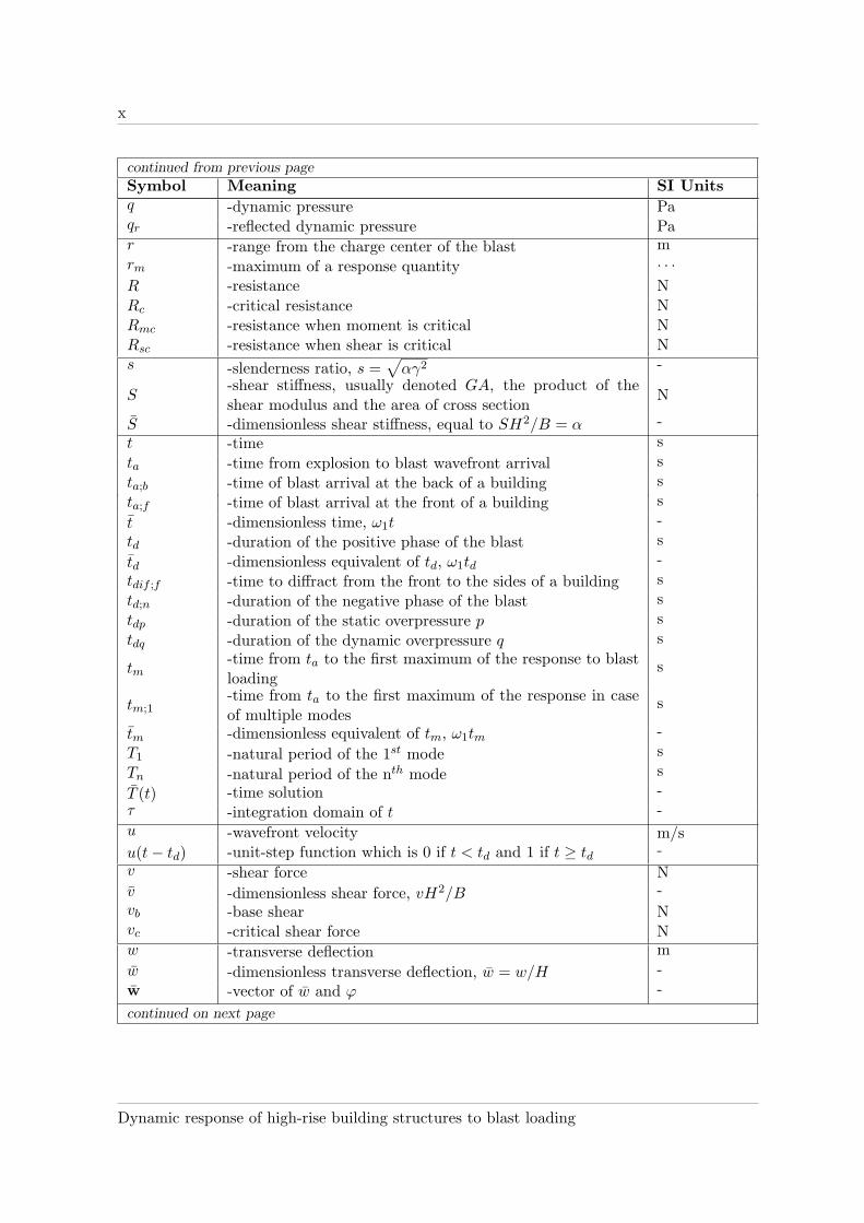
List of symbols
The list of symbols is shown below in alphabetical order, small letters first, then captives andthen Greek symbols. If a is a symbol, time derivatives of a are denoted by a and a, while spacederivatives of a are denoted by a′ and a′′. If b is a dimensional symbol, the dimensionlessequivalent is written as b. If A is a vector or matrix, it is displayed as A.
Table 1: List of symbols
Symbol Meaning SI Units
a -first wave number for the eigenfunction of a beam, 2π timesthe number of cycles in the beam length
-
ac -critical wave number, see (5.10) -an -first wave number a of the nth mode -
A -area of a cross section m2
Ab -area of cross section of beam m2
Ac -area cross section of column m2
Ad -area cross section of diagonal m2
α -dimensionless ratio of shear stiffness and bending stiffness,SH2/B = s2/γ2
-
αi-angle of incidence between a blast wavefront and the surfaceof an object, see figure 6.1
o
b-second wave number for the eigenfunction of a beam, notphysically interpretable
-
bn -second wave number b of the nth mode if a ≤ ac-
bn -second wave number b of the nth mode if a > ac-
β-dimensionless ratio of rotary spring stiffness and bendingstiffness, CH/B
-
B-bending stiffness, usually denoted as EI, the product ofYoung’s modulus and the second moment of area of thebeam cross section
Nm2
cn -modal contribution factor in the nth mode -cn;bm -modal contribution factor in the nth mode for base moment -cn;bs -modal contribution factor in the nth mode for base shear -
continued on next page
Dynamic response of high-rise building structures to blast loading

vii
continued from previous page
Symbol Meaning SI Units
C -damping constant Ns/mCc -critical damping constant Ns/mC1 − C4 -constants -
Cd -drag factor for blast wind (dynamic pressure) on an object -
Cd;b -drag factor for blast wind on the back of an object (suction) -
Cd;f -drag factor for blast wind on the front of an object -
Cφ -rotary stiffness of the foundation of a building Nm/rad
Cr-reflection factor for a blast wave on an infinite plane, seefigure 2.6
-
χb -part of deflection which is due to bending -χs -part of deflection which is due to shear -
d -length of the diagonal in a trussed frame m
D1 − D4 -constants -
D(t)-time dependent dynamic load factor (DLF), y(t)/Fm =ym(t)/yst;m
-
Ddet(t) -dynamic load factor for idealized detonation -
Dimp(t) -impulsive dynamic load factor -
Dm -maximum of time dependent dynamic load factor -
Dm;n -approximate maximum dynamic load factor in nth mode -
Dm;qs -maximum dynamic load factor in quasi-static regime -
δnm -Kronecker delta, equal to 1 if n=m, 0 otherwise -
E -Young’s modulus N/m2
Ek -kinetic energy JEs -strain energy JEw -work done Jε -correction factor for the SRSS rule applied to blast loading -ηc;buc -buckling factor for column of trussed frame -ηd;buc -buckling factor for diagonal of trussed frame -
ηn(t) -time solution within the nth mode -
f(t) -time function -
f(x) -space function -
fn -nth natural frequency Hzfy -yield stress N/m2
F -force N
F (t) -forcing function or force-time profile N
F (t) -dimensionless forcing function, F (t)/Fm -
Feq -equivalent force NFm -maximum of forcing function N
Fm -dimensionless maximum of forcing function, Fm/Rc -
Fm;mc -quasi-static asymptote when moment is critical NFm;sc -quasi-static asymptote when shear is critical N
continued on next page
L. J. van der Meer

viii
continued from previous page
Symbol Meaning SI Units
Fn -participation factor of the nth mode,∫ 10 Wm(x)P (x)dx -
G -shear modulus N/m2
γ -material property, γ =√
2(1 + ν)/k′ -
h -story height m
H -building height m
i -impulse of p∆t Pa·sin -impulse of the negative phase of the blast Pa·sir -reflected impulse Pa·sI -impulse of F∆t N·sI -dimensionless impulse, Iω1/Rc -
Ieq -equivalent impulse N·sImc -impulsive asymptote when moment is critical N·sIsc -impulsive asymptote when shear is critical N·sIz
-second moment of area of the cross section about the weak(z-)axis
m4
j -imaginary unit, j2 = −1 -
J -impulse of force per unit length Ns/mJmc -impulse per unit length when moment is critical Ns/mJsc -impulse per unit length when shear is critical Ns/m
k -integer, k = 1, 2, . . . , -
k′ -shear shape factor, k′ ≈ 1 -
K -spring stiffness N/mKb -spring stiffness which represents only bending deflection N/mKeq -equivalent spring stiffness N/mKL -load factor, equation (3.7) -
KLM -load-mass factor, KM/KL -
KM -mass factor, equation (3.5) -
KR -resistance factor, equation (3.6), but also KR = KL -
Ks -spring stiffness which represents only shear deflection N/m
` -lever between columns in trussed frame m
L -length of building in direction of blast wave propagation m
L() -stiffness operator, see equation (5.23) -
λi-modification factor for impulsive asymptote for inclusion ofhigher modes
-
λqs-modification factor for quasi-static asymptote for inclusionof higher modes
-
m -distributed mass kg/mm -dimensionless distributed mass, mH4ω2
1/B -
M -concentrated mass, mH kg
M() -mass operator, equation (5.23) -
Meq -equivalent mass kg
continued on next page
Dynamic response of high-rise building structures to blast loading

ix
continued from previous page
Symbol Meaning SI Units
MTNT -charge mass kg TNTµ -moment Nmµ -dimensionless moment, µH/B -µb -base moment Nmµc -critical moment Nmn -integer, n = 1, 2, . . . , -
Nc;c -critical axial force for a column in a trussed frame NNc;d -critical axial force for a diagonal in a trussed frame NNw -axial force in a column due to the weight of the upper stories Nν -Poisson constant, ν = 0.3 for steel -
ωn -natural circular frequency of mode n rad/sωn -dimensionless natural circular frequency, ωn/ω1 -ωζ -damped natural circular frequency rad/sp -static overpressure Pap0 -ambient pressure, at sea level p0 = 101.3 kPa Papdif -translational pressure due to static overpressure Papdrag -translational pressure due to dynamic pressure Papm -maximum static overpressure Papm;n -maximum under-pressure in negative phase of blast Papr -reflected overpressure Papr;st -reflected static overpressure Pa
ptrans-translational pressure, resultant pressure on a building orobject
Pa
P (x) -distributed load N/m
P (x) -dimensionless distributed load, P = PH3/B -
P -load vector containing force and moment -
P (x)-dimensionless distributed load divided by its maximum,P (x) = P (x)/Pm
-
Pl -linear distributed load N/mPm -maximum of P (x) N/m
Pm -maximum of P (x) -
Pm;mc -maximum distributed load when moment is critical N/mPm;sc -maximum distributed load when shear is critical N/mPq -quadratic distributed load N/mPu -uniform distributed load N/mϕ -angle of rotation due to bending moment rad
ϕ-dimensionless angle of rotation due to bending moment,equal to ϕ
rad
Ψ(x)-eigenfunction or mode shape for angle of rotation due tobending moment
-
continued on next page
L. J. van der Meer
x
continued from previous page
Symbol Meaning SI Units
q -dynamic pressure Paqr -reflected dynamic pressure Par -range from the charge center of the blast mrm -maximum of a response quantity . . .
R -resistance NRc -critical resistance NRmc -resistance when moment is critical NRsc -resistance when shear is critical Ns -slenderness ratio, s =
√
αγ2 -
S-shear stiffness, usually denoted GA, the product of theshear modulus and the area of cross section
N
S -dimensionless shear stiffness, equal to SH2/B = α -
t -time s
ta -time from explosion to blast wavefront arrival s
ta;b -time of blast arrival at the back of a building s
ta;f -time of blast arrival at the front of a building s
t -dimensionless time, ω1t -
td -duration of the positive phase of the blast s
td -dimensionless equivalent of td, ω1td -
tdif ;f -time to diffract from the front to the sides of a building s
td;n -duration of the negative phase of the blast s
tdp -duration of the static overpressure p s
tdq -duration of the dynamic overpressure q s
tm-time from ta to the first maximum of the response to blastloading
s
tm;1-time from ta to the first maximum of the response in caseof multiple modes
s
tm -dimensionless equivalent of tm, ω1tm -
T1 -natural period of the 1st mode s
Tn -natural period of the nth mode s
T (t) -time solution -τ -integration domain of t -
u -wavefront velocity m/su(t − td) -unit-step function which is 0 if t < td and 1 if t ≥ td -
v -shear force Nv -dimensionless shear force, vH2/B -vb -base shear Nvc -critical shear force Nw -transverse deflection m
w -dimensionless transverse deflection, w = w/H -
w -vector of w and ϕ -
continued on next page
Dynamic response of high-rise building structures to blast loading

xi
continued from previous page
Symbol Meaning SI Units
W -width of the front of a building m
W (x) -eigenfunction or mode shape for transverse deflection -
Wn -vector of Wn and Ψn of the nth mode -
Wm
T -transpose of Wm-
x -axial coordinate from bottom x = 0 to top x = H of beam m
x -dimensionless equivalent of x, x/H -
y -transverse deflection m
y -transverse velocity m/sy -transverse acceleration m/s2
y -dimensionless transverse deflection y = y/yc -
˙bary -dimensionless transverse velocity ˙bary = y/(ω1yc) -
yb -bending deflection myc -critical deflection myc;e -critical elastic deflection myc;p -critical plastic deflection myl -deflection due to linear load distribution mym -maximum dynamic deflection mym;st -maximum static deflection, Fm/K m
ym -maximum transverse velocity m/symc -deflection when moment is critical myq -deflection due to quadratic load distribution myr -deflection due to rotation of the base mys -deflection due to shear mysc -deflection when shear is critical myu -deflection due to uniform load distribution m
z -scaled distance, r/(MTNT )1/3 kg/m1/3
ζ -damping ratio, C/Cc -
L. J. van der Meer

xii
Contents
Acknowledgements i
Summary ii
Nederlandse samenvatting iv
List of Symbols vi
1 Introduction 1
1.1 Problem statement . . . . . . . . . . . . . . . . . . . . . . . . . . . . . . . . . 2
1.2 State of the art . . . . . . . . . . . . . . . . . . . . . . . . . . . . . . . . . . . 2
1.2.1 Guidelines . . . . . . . . . . . . . . . . . . . . . . . . . . . . . . . . . . 2
1.2.2 Research . . . . . . . . . . . . . . . . . . . . . . . . . . . . . . . . . . . 2
1.3 Research outline . . . . . . . . . . . . . . . . . . . . . . . . . . . . . . . . . . 3
2 Explosion, blast and interaction 7
2.1 Explosive loading . . . . . . . . . . . . . . . . . . . . . . . . . . . . . . . . . . 7
2.2 Blast loading . . . . . . . . . . . . . . . . . . . . . . . . . . . . . . . . . . . . 8
2.2.1 Pressure-time profile . . . . . . . . . . . . . . . . . . . . . . . . . . . . 8
2.2.2 Scaled distance . . . . . . . . . . . . . . . . . . . . . . . . . . . . . . . 9
2.2.3 Dynamic blast pressure . . . . . . . . . . . . . . . . . . . . . . . . . . 10
2.3 BLEVE blast loading . . . . . . . . . . . . . . . . . . . . . . . . . . . . . . . . 10
2.3.1 Blast wave from a vessel burst . . . . . . . . . . . . . . . . . . . . . . 11
2.3.2 Blast wave from a BLEVE . . . . . . . . . . . . . . . . . . . . . . . . 12
2.4 Blast-structure interaction . . . . . . . . . . . . . . . . . . . . . . . . . . . . . 12
2.4.1 Blast waves on an infinite rigid plane . . . . . . . . . . . . . . . . . . . 12
2.4.2 Blast waves on a building . . . . . . . . . . . . . . . . . . . . . . . . . 13
2.4.3 Blast distribution . . . . . . . . . . . . . . . . . . . . . . . . . . . . . . 17
3 Modeling of high-rise building structures 19
3.1 Example of a realistic building structure . . . . . . . . . . . . . . . . . . . . . 20
3.2 A stability element: the trussed frame . . . . . . . . . . . . . . . . . . . . . . 20
3.3 The equivalent beam . . . . . . . . . . . . . . . . . . . . . . . . . . . . . . . . 21
3.4 The equivalent single degree of freedom system . . . . . . . . . . . . . . . . . 22
3.4.1 Load-mass factors for slender beams . . . . . . . . . . . . . . . . . . . 25
3.4.2 Load-mass factors for simple shear beams . . . . . . . . . . . . . . . . 27
3.4.3 Load-mass factors for non-slender beams . . . . . . . . . . . . . . . . . 28
Dynamic response of high-rise building structures to blast loading

CONTENTS xiii
3.4.4 Load-mass factors for non-slender beams with rotary spring . . . . . . 29
3.4.5 Comparison of models . . . . . . . . . . . . . . . . . . . . . . . . . . . 30
4 Dynamic response of a SDOF system to blast loading 33
4.1 Dynamic response of SDOF systems to idealized blast loading . . . . . . . . . 34
4.1.1 Natural frequency of vibration . . . . . . . . . . . . . . . . . . . . . . 35
4.1.2 Damping . . . . . . . . . . . . . . . . . . . . . . . . . . . . . . . . . . 35
4.1.3 Material model . . . . . . . . . . . . . . . . . . . . . . . . . . . . . . . 36
4.1.4 Forcing function . . . . . . . . . . . . . . . . . . . . . . . . . . . . . . 36
4.1.5 Response to idealized blast loads . . . . . . . . . . . . . . . . . . . . . 37
4.2 Time of maximum deflection and the dynamic load factor . . . . . . . . . . . 39
4.2.1 Time of maximum deflection . . . . . . . . . . . . . . . . . . . . . . . 41
4.2.2 The dynamic load factor . . . . . . . . . . . . . . . . . . . . . . . . . . 42
4.2.3 Limits of the dynamic load factor . . . . . . . . . . . . . . . . . . . . . 43
4.3 The pressure-impulse diagram . . . . . . . . . . . . . . . . . . . . . . . . . . . 45
4.3.1 Pressure-impulse diagrams in literature . . . . . . . . . . . . . . . . . 46
5 Dynamic response of a continuous beam to blast loading 49
5.1 The differential equation of motion of a transversely vibrating Timoshenko beam 50
5.1.1 Dimensionless variables . . . . . . . . . . . . . . . . . . . . . . . . . . 50
5.1.2 Equation of motion of a Timoshenko beam . . . . . . . . . . . . . . . 50
5.2 Determination of mode shapes and natural frequencies of a beam . . . . . . . 51
5.3 The mode superposition method: forced response of a beam . . . . . . . . . . 52
5.3.1 Orthogonality and normalization of eigenfunctions . . . . . . . . . . . 53
5.3.2 Mode superposition method . . . . . . . . . . . . . . . . . . . . . . . . 54
5.3.3 Modal contribution factors . . . . . . . . . . . . . . . . . . . . . . . . 56
5.4 Approximation of response including higher modes . . . . . . . . . . . . . . . 59
5.4.1 Modal combination rules . . . . . . . . . . . . . . . . . . . . . . . . . . 59
5.4.2 Dynamic load factor including higher modes . . . . . . . . . . . . . . . 60
5.4.3 Estimates of maximum response . . . . . . . . . . . . . . . . . . . . . 66
5.5 Pressure-impulse diagram including higher modes . . . . . . . . . . . . . . . . 66
6 Results for example building structure 69
6.1 BLEVE blast loading on example building . . . . . . . . . . . . . . . . . . . . 69
6.1.1 Blast distribution . . . . . . . . . . . . . . . . . . . . . . . . . . . . . . 70
6.2 Modeling of example building structure . . . . . . . . . . . . . . . . . . . . . 71
6.2.1 From trussed frame to equivalent beam . . . . . . . . . . . . . . . . . 72
6.2.2 From equivalent beam to equivalent SDOF system . . . . . . . . . . . 72
6.3 Single degree of freedom response . . . . . . . . . . . . . . . . . . . . . . . . . 73
6.3.1 Pressure-impulse diagram for SDOF response . . . . . . . . . . . . . . 75
6.4 Response of a continuous beam . . . . . . . . . . . . . . . . . . . . . . . . . . 76
6.4.1 Pressure-impulse diagram including higher modes . . . . . . . . . . . . 77
6.5 Comparison of results . . . . . . . . . . . . . . . . . . . . . . . . . . . . . . . 78
6.5.1 Comparison of response . . . . . . . . . . . . . . . . . . . . . . . . . . 78
6.5.2 Comparison of p − i− diagram . . . . . . . . . . . . . . . . . . . . . . 78
6.5.3 Modification factors for inclusion of higher modes . . . . . . . . . . . . 78
L. J. van der Meer

xiv CONTENTS
7 Conclusions 83
8 Recommendations 87
A Matlab input files 89
A.1 Pressure-impulse diagram (SDOF) . . . . . . . . . . . . . . . . . . . . . . . . 89A.2 Wave numbers of a Timoshenko beam . . . . . . . . . . . . . . . . . . . . . . 91
B Ansys input files 93
References 101
Dynamic response of high-rise building structures to blast loading

1
Chapter 1
Introduction
This report is about the dynamic response of high-rise building structures to blast loading ingeneral and BLEVE blast loading in particular. In this chapter, a topical problem is statedconcerning BLEVE blast loading on high-rise building structures. Subsequently the state ofthe art is described, including rules, guidelines and ongoing research. Then an outline of theresearch underlying this report is presented.
In chapter 2 the effects of an explosion and in particular of a blast on a building structureare described. The chapter does not go into detail about the causes of an explosion nor aboutthe physical and chemical circumstances. The blast wave produced by an explosion is studiedin terms of pressure in the free field. Finally the influence of obstructions such as buildingson the blast wave pressures is illustrated.
Chapter 3 is dedicated to the modeling of a realistic, but simple building structure insteps of decreasing complexity. After the building structure has been presented, it is reducedto a single stability element, a trussed frame. The stability element is further reduced to anequivalent beam. The final model is a single-degree-of-freedom (SDOF) spring mass system.Every step of modeling is described in detail and the assumptions necessary for each step aregiven.
Succeeding chapter 3, in which the SDOF system describing the building structure hasbeen established, chapter 4 focusses on the dynamic response of the SDOF system. Thedifference between static and dynamic response is explained and concepts of dynamic loadfactor (DLF) and pressure-impulse (p-i-)diagram are introduced.
The response of a SDOF system is only useful if the assumptions made during the steps ofmodeling are acceptable. An important lack of the SDOF system is the fact that higher modesof vibration are ignored. Therefore, chapter 5 moves up one step in the modeling process bydetermining the response of a continuous beam with infinite degrees of freedom. First thetype of beam is determined, then the equation of motion is given and the mode shapes andnatural frequencies are obtained. The forced response of the continuous beam is determinedwith the mode superposition method. Special attention is given to modal contribution factorsfor base shear and moment, which give the percentage of participation of a certain mode.The maxima of the time dependent base shear and moment are approximated using modalcombination rules and assumptions regarding the dynamic load factor of the higher modes ofvibration. The pressure-impulse diagram is constructed using these approximation includinghigher modes of vibration.
In chapter 6, the response of the example building structure, which is modeled in chapter
L. J. van der Meer

2 Chapter 1: Introduction
3 as a continuous beam and a SDOF system, is determined with and without higher modesof vibration using the methods described in chapters 5 and 4 respectively. The p-i diagramsof both models are compared and the location in the diagram of a BLEVE blast accordingto both Dutch guidelines and more recent research is given in order to assess damage of thestructure.
Conclusions and recommendations are given in chapter 7 and 8 respectively.
1.1 Problem statement
In the Netherlands, residential and office buildings near the railway line from the Rotterdamharbor to Germany, risk being struck by a BLEVE. A BLEVE is a type of explosion that canoccur when a train wagon containing a liquified gas is damaged. It is described in more detailin section 2.3. A case study including risk assessment was done on this particular problem bySjoerd Mannaerts, another graduation student from Eindhoven University of Technology. Thegraduation project of Sjoerd Mannaerts (2008) focussed on risk assessment and blast wavepropagation. This graduation project focusses on the dynamic response of high-rise buildingstructures to explosive loading. Different types of loading from an explosion are described inchapter 2. First the state of the art in the Netherlands, Europe and worldwide is reviewedand an outline of the research project is presented, including limitations.
1.2 State of the art
Guidelines, rules and ongoing research in the field of explosion effects on building structuresin the Netherlands, in Europe and worldwide, are reviewed in this section.
1.2.1 Guidelines
In the Netherlands, the Ministry of Housing, Spatial Planning and the Environment, haspublished a series of documents about toxic and hazardous substances. One part of this seriesis about explosion effects on structures [22]. It describes idealized blast loads, blast-structureinteraction, the response of single-degree-of-freedom (SDOF) systems to blast loading, thedynamic load factor, pressure-impulse diagrams, the translation of a structure to a SDOFdynamic model, the strength of glass windows, debris and the use of empirical data basedon explosive events during the Second World War. Empirical data is only valid for buildingstructures up to four stories. For building structures of more than four stories, schematizationas a SDOF system is suggested. The explosion itself is described in Chapter 5 of [23].
The Dutch guideline [22] is partly based on [3], an American manual about Structures toresist the effect of accidental explosions by the US Army, Navy and Air Force. The manualis almost 1800 pages thick and contains information about blast, fragment and shock loads,principles of dynamic analysis, reinforced concrete design and structural steel design withrespect to explosive loading.
1.2.2 Research
Explosion resistance was part of a workshop in Prague, March 2007, by the European Coop-eration in the Field of Scientific and Technical Research, titled Urban Habitat Constructions
Dynamic response of high-rise building structures to blast loading
1.3 Research outline 3
under Catastrophic Events [24]. In one of the papers [18] collected in this reference, currentresearch in the area of impact and explosion engineering is summarized and categorized:
• Whole building and building element response and robustness in the face of blast andimpact loading. Robustness is defined as the resistance of the structure to progressivecollapse due to local damage;
• Response of structures to blast loads from both high explosive events and gas explosionsusing experimental and numerical methods;
• Response of buildings to underground explosions and the utility of seismic designmethodologies to produce blast and impact resistant structures;
• Response of structures and structural elements to impact from missiles and vehicles;
• Development of existing expertise in general ’dynamic loading’ towards impact andexplosion studies.
In another paper [11] from the same reference, future research that is required in the areaof impact and explosion engineering is described. The paper is based mainly on terrorism,but could be applied to explosions from other causes as well. Existing design manuals, forexample [3], are listed and commented upon. According to the article, future research shouldinclude among others:
• Protection methodology and risk assessment.
• Load and environment definition.
• Material behavior.
• Computational capabilities.
• Behavior and effects of building enclosure.
• Building and structural behavior.
• Combined knowledge of explosion, earthquake and wind engineering.
The author also states that ’the traditional concept of pressure-impulse diagrams should bere-evaluated’(p. 287 of [11]), without explaining why. However, a recent article [12] by thesame author about the numerical determination of the pressure-impulse (p-i) diagram makesclear that he thinks of p-i diagrams as a useful tool for damage assessment of structuralcomponents and wants to overcome the limitations of the analytical determination of thesediagrams.
1.3 Research outline
Objectives of the research project are:
• Verify the assumption that high-rise buildings can be analyzed for blast loading as aSDOF system.
L. J. van der Meer
4 Chapter 1: Introduction
• Apply the concept of pressure-impulse diagram to high-rise building structures.
• Model a high-rise building with different levels of complexity and predict response toblast loading.
• Include higher modes in the p-i diagram.
• Compare results.
A framework is presented in figure 1.1. The research projects focusses on the modeling (fromactual structure to (discrete) FE model to continuous model to SDOF model) and the pseudo-analytical part. It is called pseudo-analytical because some parts of the analysis such as thedetermination of the mode shapes and natural frequencies of the continuous model can onlybe done with help of numerical software, depending on beam type and boundary conditions.Also, if p-i diagrams for a complex material model and load-time history are needed, nu-merical methods are necessary. The structural variables material model and damping arebetween brackets, because the material model is linear-elastic throughout this investigationand damping is ignored (conservative). The part concerning coupled numerical response isshown in dashed lines, because it is not within the scope of this research project. An exampleof this approach can be found in [15].
Dynamic response of high-rise building structures to blast loading

1.3 Research outline 5
Act
ual
Couple
dnum
eric
al
Unco
uple
dnum
eric
al
Pse
udo-A
naly
tica
l
Act
ualbla
st
-lit
eratu
re-(
exper
imen
ts)
-CFD
Couple
dFE
model
ofbla
stand
stru
cture
Bla
stva
riable
-idea
lise
dbla
stlo
ad
Str
uct
ura
lva
riable
s
-fre
quen
cyra
tio
-sle
nder
nes
sra
tio
-(m
ate
rialm
odel
)-(
dam
pin
g)
Act
ual
stru
cture
FE
stru
ctura
lm
odel
-2D
-3D
Conti
nuous
model
SD
OF
model
Act
ual
resp
onse
Couple
dre
sponse
Num
eric
al
MD
OF
resp
onse
Conti
nuous
∞D
OF
resp
onse
-p−
i−dia
gra
m
SD
OF
resp
onse
-p−
i−dia
gra
m
Com
ple
xSim
ple
model
ing
idea
liza
tion
inte
ract
ion
mod
eling
model
ing
model
ing
model
ing
couple
dtr
ansi
ent
dynam
icanaly
sis
exper
imen
tstr
ansi
ent
analy
sis
mode
super
posi
tion
analy
sis
(analy
tica
l)
com
pare
com
pare
ass
um
pti
ons
dis
trib
uti
on
analy
tica
l
Figure 1.1: Framework of graduation project.
L. J. van der Meer


7
Chapter 2
Explosive loading, blast loading andblast-structure interaction
In this chapter, explosive loading is described. In section 2.1, different types of loading on abuilding structure, caused by an explosion are described. The blast wave, one of these typesof loading, is described in more detail in section 2.2. It is the only load effect considered in therest of the report. Special attention is given to blast from a BLEVE in section 2.3. In section2.4, the influence of a building structure as a rigid object on the blast wave is illustrated andthe blast loading on the building structure is given in terms of pressure and impulse.
2.1 Explosive loading
Explosion effects on building structures can be divided into primary and secondary effects.The primary effects include:
1. Airblast: the blast wave causes a pressure increase of the air surrounding a building struc-ture and also a blast wind. More attention to this phenomena will be given in section2.2.
2. Direct groundshock: an explosive which is buried completely or partly below the groundsurface, will cause a groundshock. This is a horizontal (and vertical, depending on thelocation of the explosion with regard to the structural foundation) vibration of the ground,similar to an earthquake but with a different frequency.
3. Heat: a part of the explosive energy is converted to heat. Building materials are weakenedat increased temperature. Heat can cause fire if the temperature is high enough.
4. Primary fragments: fragments from the explosive source which are thrown into the airat high velocity (for example wall fragments of an exploded gas tank). Fragments canhit people or buildings near the explosion. They are not a direct threat to the bearingstructure of the building, which is usually covered by a facade. However, they may destroywindows and glass facades and cause victims among inhabitants and passers-by.
An overview of the explosion effects on buildings, summarized by the author of this report,is given in figure 2.1. Secondary explosion effects, such as secondary fragments and blast-induced groundshock are not considered.
L. J. van der Meer

8 Chapter 2: Explosion, blast and interaction
-target shape-blast propagation-environment
-natural frequencies-material properties-static strength-dimensions-robustness-damping-ductility
1. AirblastStructure
above ground
Overallstructuralresponse
Explosion
-charge mass-type of explosion-location
2. Groundshock Foundation
3. Heat
Facade/Exposedstructuralelements
Localdamage
4. Fragments
air
ground baseexcitation
air
impac
t
interaction
Figure 2.1: Explosion effects on structures.
2.2 Blast loading
An elaborate description of explosions and blast waves is given in reference [19] of which someparts that are relevant to this report are explained below.
During an explosion an oxidation reaction occurs that is called combustion. When ex-plosive materials decompose at a rate below the speed of sound (subsonic), the combustionprocess is called deflagration. Gas and dust explosions are of this type. Under specific con-ditions a deflagration to detonation transition can occur. Detonation is the other form ofreaction which produces a high intensity shock wave. The reaction rate is 4-25 times fasterthan the speed of sound (supersonic). An explosion of TNT is an example of a detona-tion. The two types of explosions have significantly different pressure-time profiles and willtherefore be treated separately in this report.
2.2.1 Pressure-time profile
The meaning of a few important blast parameters can be seen in figure 2.2. In this figure, tais the arrival time of the blast, td is the positive (overpressure) phase duration of the blast,
Dynamic response of high-rise building structures to blast loading

2.2 Blast loading 9
td;n is the negative (under-pressure i.e. negative overpressure) phase duration of the blast,p0 is the ambient pressure, pm is the peak static overpressure, pn;m is the maximum valueof under-pressure, i is the impulse of the positive phase of the pressure-time curve and in isthe impulse of the negative phase of the pressure-time curve. The pressure-time profile inthe figure is that of a detonation. The deflagration pressure-time profile is different as canbe seen in figure 2.3. The deflagration pressure-time profile will transform to a detonationprofile if the peak-static overpressure exceeds the value of approximately 3kPa (pm > 3 kPa).
t
ta
td td;n
p(t)
pm
p0
pn;m
Area = i
Area = in
Figure 2.2: Blast wave pressure time profile, taken from [19].
t
p(t)
pm i
(a) Detonation
t
p(t)
pm
(b) Deflagration
Figure 2.3: Detonation and deflagration pressure-time history.
2.2.2 Scaled distance
An important parameter for determination of air-blast pressure and impulse is the scaleddistance z, which is dependent of the distance r from the charge center in meters and thecharge mass MTNT expressed in kilograms of TNT:
z =r
(MTNT )1/3(2.1)
Other blast parameters can conveniently be plotted against the scaled distance. Such graphscan be found in reference [3]. In figure 2.4 the peak static overpressure p, impulse i, time of
L. J. van der Meer

10 Chapter 2: Explosion, blast and interaction
0.01
0.1
1
10
100
1000
10000
100000
1000000
0.01 0.1 1 10 100
z[m/kg1
3 ]
p[kPa]
i[kPa · ms/kg1
3 ]
td[ms/kg1
3 ]
ta[ms/kg1
3 ]
p i
ta ta + td
Figure 2.4: Blast parameters for TNT equivalent explosions [3]
blast arrival ta and positive phase duration td are shown depending on the scaled distance z.
2.2.3 Dynamic blast pressure
Apart from a static overpressure p, there is also a dynamic pressure q (i.e. blast wind)associated with a blast wave. This dynamic pressure is higher than the static overpressurefor small scaled distance and lower than the static overpressure for large scaled distance.The positive phase duration of the dynamic pressure tdq and static overpressure tdp is alsodifferent, but in this report it will be assumed that both durations are equal. In figure 2.5 thestatic overpressure p and the dynamic pressure q are displayed versus the scaled distance z.
2.3 BLEVE blast loading
BLEVE is an abbreviation for boiling liquid expanding vapor explosion. According to [5], aBLEVE is the explosive release of expanding vapor and boiling liquid when a container holdinga pressure-liquified gas fails catastrophically. Catastrophic failure means that the containeris fully opened to release its contents nearly instantaneously. This total loss of containmentcan take place for a number of reasons including flawed materials, fatigue, corrosion, poormanufacture, thermal stresses, pressure stresses and reduction in material strength due tohigh wall temperatures. Other definitions state that the liquid temperature must be above theatmospheric superheat limit, but BLEVEs were also observed for liquid temperatures beneaththis limit. However if the material is a pressure-liquified gas, its temperature at atmosphericpressure must be above the superheat limit if explosive boiling is to occur. According to [1]a BLEVE gives rise to the following:
• Splashing of some of the liquid to form short-lived pools, which would be on fire if theliquid is flammable.
• Blast wave.
Dynamic response of high-rise building structures to blast loading

2.3 BLEVE blast loading 11
0.01
0.1
1
10
100
1000
10000
100000
1000000
0.01 0.1 1 10 100
472kPa
z[m/kg1
3 ]
q[kPa]
p[kPa]
tdp tdq
pq
Figure 2.5: Static overpressure p vs dynamic pressure q [3].
• Flying fragments (’missiles’).
• Fire or toxic gas release. If the pressure-liquified vapor is flammable, as is often thecase, the BLEVE leads to a fireball. When the material undergoing BLEVE is toxic,adverse impacts include toxic gas dispersion.
A list of BLEVE accidents is also available in reference [1]. The accidents concern for exampleroad and rail transport of pressure-liquified gasses (PLGs) or storage of PLGs at petrolstations or near factories/plants. The worst BLEVE accident occurred in 1984 in MexicoCity and was responsible for 650 deaths and over 6400 injured.
2.3.1 Blast wave from a vessel burst
In this report, only the blast wave produced by the BLEVE is considered. It should be notedthat the other effects can do significant damage to buildings and people near to or in them.In the Netherlands the methods for calculating blast effects from vessel bursts in general aredivided in two categories (paragraph 7.3.2 of [23]):
• Methods of solving the differential equations of fluid mechanics by which the shock wavecan be described. Analytical solving is only possible when a lot of simplifications aremade. Numerical solving can be done by means of finite-difference methods or Eulerian-Lagrangian codes. However, these methods require a lot of knowledge and give resultsfor specific situations.
• Generalized methods based on thermodynamic terms and the available energy for blastgeneration. Two methods developed in this category are described.
1. The first method is based on high explosives, for which the blast effects are known.Unfortunately, blast effects from vessel bursts include lower initial overpressures,a slower decay of the overpressure with distance, longer positive phase durations,much larger negative phases and strong secondary shocks. This method gives
L. J. van der Meer
12 Chapter 2: Explosion, blast and interaction
reasonable results only at far range, which means larger than 10-20 times thevessel diameter.
2. The second method is Baker’s method, based on research by W. E. Baker in 1977,which is comparable to the previous method at far range. At close range experi-mentally verified results for ideal gasses are used. The method includes a correctionmethod for the influence of a nearby surface and the shape of the vessel.
2.3.2 Blast wave from a BLEVE
For a BLEVE, which is a special case of a vessel burst, Baker’s method includes a modificationfor vessels with flashing liquids. In [23] this last method is selected and described in paragraph7.5.2 and in the example on page 7.63. The method might be non-conservative because itresults in too short positive phase durations.
More recently, in [21], a new method to calculate the blast effects from BLEVE wasintroduced. By using acoustic blast modeling, it was found that the blast effects dependstrongly upon the exact release and evaporation rate of the liquified gas. If it is assumed thatthe pressure vessel nearly instantaneously disintegrates, then the release rate approximatesinfinity and the evaporation rate of the superheated liquid is fully determined by the rate atwhich the developing vapor can expand by moving the mass of vapor and the surroundingair. This is called expansion-controlled evaporation. The assumption of nearly instantaneousdisintegration is conservative. In [21], BLEVE blast charts for propane in half space areshown, which are determined by gas dynamic modeling using the assumption of expansion-controlled evaporation. Compared to Baker’s method, presented in [23], the blast parametersare less conservative. It should be noted that the modification factors for a nearby surfaceand the shape of the vessel are not included in the blast parameters of [21]. This meansthat the parameters are valid for a hemispherical blast originating at the surface. When themodification factors are applied to Van den Berg’s method, the overpressures are similar tothose of Baker’s method for far range and the positive phase durations (and consequentlyimpulses) are larger.
In this report both a BLEVE following [23] and [21] will be used in example calculations.
2.4 Blast-structure interaction
Blast parameters are given in literature for TNT blasts in free space (free-air burst) or halfspace (surface burst). In case of a surface burst, parameters for free-air bursts should bemultiplied by a reflection factor of 1.8 [19]. Theoretically this factor should equal 2, but someenergy is dissipated in the deformation of the surface. A reflection factor of 1.8 gives goodagreement with experimental results.
2.4.1 Blast waves on an infinite rigid plane
If a blast wave with a certain (time dependent) static overpressure p(t), dynamic pressure q(t)and impulse i(t) encounters an infinite, rigid plane, it is reflected. Because the incident waveand the reflected wave coincide, the pressure on the rigid plane is higher than the pressure ofthe incident wave and is denoted pr(t), reflected overpressure. The reflected impulse associatedwith the reflected overpressure is denoted ir(t).
Dynamic response of high-rise building structures to blast loading

2.4 Blast-structure interaction 13
The reflected overpressure and impulse are dependent on the angle of incidence αi ofthe blast wave, which is the angle between the blast wavefront and the target surface. Thereflection coefficient Cr is defined as the ratio of the reflected overpressure and the incidentoverpressure (overpressure if the wave were not obstructed, sum of static overpressure p(t)and dynamic pressure q(t)). If the angle of incidence is 90o, the blast wave travels alongsidethe plane and the overpressure is equal to the static overpressure, which is also referred toin literature as side-on overpressure. The dynamic pressure q(t) works in this case only inthe direction parallel to the plane and is therefore (almost) not obstructed. The frictionbetween the moving air and the rigid plane is negligible. For all αi between 0 − 90o, thereflected pressure pr(t) is dependent on the static overpressure p(t) and the dynamic pressureq(t). The reflection coefficient Cr is shown versus the angle of incidence αi in figure 2.6 fora detonation. As the figure points out, the reflection coefficient is dependent on the staticoverpressure p(t). The reflection coefficient also depends on the type of explosion, detonationor deflagration. For a deflagration, figures are available in [3] and [22].
Starting at an angle of incidence αi of approximately 40o, depending on the static over-pressure, the reflection coefficient Cr increases and has a local maximum which is sometimeshigher than the reflection coefficient at αi = 0o. This is due to Mach reflection, which occurswhen the reflected wave catches up and fuses with the incident wave at some point abovethe reflecting surface to produce a third wavefront called the Mach stem [19]. According to[22], these local peak values are the result of theoretical derivations that could not be verifiedby experiments. Therefore it is suggested that these peak values are flattened for simplecalculations.
2.4.2 Blast waves on a building
If a blast wave encounters a building, the building is loaded by a pressure, which is a sum-mation of two parts: the first part is due to the static overpressure and the second part isdue to the dynamic pressure or blast wind. These pressures are shown in figure 2.7. Bothstatic overpressure and dynamic pressure are a function of time, but also of the unobstructeddistance to the charge center. Time and distance are coupled by the velocity at which theblast wave is propagating, although this velocity is not constant.
Due to the coupling of time and distance, the part of translational pressure ptrans(t) whichis due to the static overpressure p(t) depends on the size of the building (or other object)compared to the positive phase duration of the blast td. The translation pressure is definedas the nett pressure due to blast loading.
If the building is very small in one direction (width or height), the overpressure on thefront and the back of the building is approximately equal and hence the translational pressureis approximately zero (figure 2.8a, overpressure).
If the building is larger (width or height) compared to the blast duration and the angle ofincidence is 0o, the front of the building is loaded with the reflected static overpressure pr;st(t).The sides are loaded with the static overpressure. However, this pressure works in oppositedirection on both sides and does not result in translational pressure. The pressure in the blastwave traveling along the sides equals the static overpressure (dynamic pressure is consideredfurther on). This pressure is lower than the reflected static overpressure, which causes largelocal pressure differences. These pressure differences cause the blast wave to diffract aroundthe building. When the diffraction from the front to the sides of the building is completed,the static pressure on the front is decreased from the reflected static overpressure to the static
L. J. van der Meer

14 Chapter 2: Explosion, blast and interaction
0
1
2
3
4
5
6
7
8
9
10
11
12
13
0 10 20 30 40 50 60 70 80 90
34474
20684
13790
6895
3447
2758
2068
1379
1034
689.5
482.5
344.7
206.8
137.9
68.95
34.47
13.79
6.895
3.447
1.379
p[kPa]
αi[o]
Cr
Figure 2.6: Reflection coefficient vs angle of incidence for a detonation (figure 3-3 from TM5-855, predecessor of [3])
overpressure. Similarly, pressure differences cause the blast wave to diffract from the sidesto the back of the building, once the blast wave front passes by the back of the building.Translational pressure resulting from diffraction is significant only when the time to diffractaround the building is approximately equal to or larger than the positive phase duration ofthe blast. For this type of building and blast, the building is called a diffraction target (figure2.8b, overpressure).
If the positive phase duration of the blast is much smaller than the time to diffract aroundthe building, the building is loaded sequentially. A sequentially loaded building feels a pressurefrom the blast wave either at the front, at the sides or at the back, but not at the same time(figure 2.8c, overpressure).
Summarizing the effects of static overpressure on a building, three essentially differenttypes can be distinguished:
• No translational pressure (long positive phase duration compared to time of diffraction).
• Translational pressure due to difference between overpressure on front and back (positivephase duration approximately equal to or larger than the time of diffraction).
• Translational pressure due to local overpressure only (small positive phase durationcompared to time of diffraction).
The effects of static overpressure determine the translational pressure on a building to-gether with effects of the dynamic pressure or blast wind. Whereas the static overpressure is
Dynamic response of high-rise building structures to blast loading

2.4 Blast-structure interaction 15
ta;f
ta;b
(a) (b)
t
p(t)
Figure 2.7: Static overpressure (a) and dynamic pressure (b) on a box-shaped target.
caused by an increased density of the air, the dynamic pressure is the result of the movementof air away from the blast source. Similar to ordinary wind, the blast wind causes a pressureon the front of a building and a negative pressure (suction) at the back of a building. Bothpressures are translational in the same direction. Because of their translational nature, thesepressure are called drag pressures. The drag pressure on a building or object is equal to thedynamic pressure multiplied by a drag factor Cd. Drag factors can be found in [22], table4-1, for loads on the front side of an object. The drag coefficient for suction at the back ofthe object is smaller and negative (Cd = −0.3 for a boxed-shape object and αi = 0o).
The dynamic pressure on the front is reflected similar to the static overpressure. In liter-ature, the reflected overpressure pr(t) includes both the reflected static overpressure pr;st(t)and the reflected dynamic pressure qr(t). This is rather confusing and leads to mistakes suchas in figure 3.27 of [19], where the drag force is superimposed on the force from the reflectedoverpressure. If a building is small (height or width), the pushing and sucking drag pres-sures on front and back are applied at approximately the same time. Because of the smalldimensions of the front face, no reflection occurs (figure 2.8a, dynamic pressure).
For the other types of buildings, the behavior is similar as for static overpressure (figure2.8b-2.8c, dynamic pressure), except for the direction of the pressure on the back of thebuilding, which is opposite of the direction of static overpressure. The reason for this similarityis found in the similarity of the pressure-time history of static overpressure and dynamicpressure.
Summarizing the effects of both static overpressure and dynamic pressure, the target(building with respect to blast) can be divided into three categories:
• Drag target: translational pressure from dynamic pressure, crushing from static over-pressure (long positive phase duration compared to time of diffraction). See figure 2.8a.
• Diffraction target: translational pressure due to both dynamic pressure and static over-pressure (positive phase duration approximately equal to or larger than time of diffrac-tion). See figure 2.8b.
• Sequentially loaded target: translational pressure due to both dynamic pressure andstatic overpressure, but only local (positive phase duration (much) smaller than time ofdiffraction). See figure 2.8c.
L. J. van der Meer

16 Chapter 2: Explosion, blast and interaction
TargetTranslational pressure Idealized
pulse shapeOverpressure Dyn. pressure
ta ta + td
wavefront
Cd;f Cd;b
ptrans(t)
(a) Drag target
Cd;f Cd;b
LW
H
ptrans;f (t)
pdrag;b(t)
pdif ;b(t)
(b) Diffraction target
Cd;f
LW
H ir
td
pr(t)
(c) Sequentially loaded target
Figure 2.8: Target categories for blast loading on a building.
Other objects near the blast source as well as inequalities in the surface all influence theblast pressure-time history. It can be concluded that a lot of information is needed about theexplosive and its location, the geometry of the target and its surroundings to be able to quan-tify the pressure-time history. In complex built environments, a lot of reflections can occur,leading to a complex pressure-time history [20]. It is impossible to calculate all reflectionsand possible re-reflections under different angles of incidence as well as the influence of thegeometry of the target and surrounding structures on the reflected overpressure analytically.In this case it is necessary to do experiments or to use CFD, Computational Fluid Dynamics,to simulate the blast. In uncoupled CFD buildings are modeled as rigid objects. In coupledCFD the influence of movement and failure of building elements on the blast wave propaga-tion is also considered. An example can be found in [15]. However, a lot of input is requiredby the user as well as expertise in finite element modeling.
Dynamic response of high-rise building structures to blast loading

2.4 Blast-structure interaction 17
2.4.3 Blast distribution
Using the knowledge from the previous sections and the methods from literature to obtainquantitative information about the translational pressure and impulse on a building, thedistribution of pressure and impulse over the facade of the building has not been taken intoaccount. For blasts at large range, the distribution is approximately uniform. At shorterranges, this assumption is not valid, since the blast propagation from a surface burst ishemispherical. At close range, the range (and scaled distance) to different heights on thefacade is significantly unequal. For example, if the building is 65m high and the range fromthe surface burst to the base of the building is 20m, the range from the surface burst to the topis 68m. This difference in range (and scaled distance) does not only result in different pressureand impulse, but also in a different arrival time ta of the blast and a different positive phaseduration td. So, by calculating the range r and scaled distance z from the blast source toevery point on the facade and taking into account the angle of incidence αi, blast parameterscan be determined using figures 2.9 and 2.6. Figure 2.9 is similar to figure 2.4, but includingthe reflected pressure pr and impulse ir. Also the wavefront speed u is shown which can beused in calculations of diffraction.
0.01
0.1
1
10
100
1000
10000
100000
1000000
0.01 0.1 1 10 100
pr[kPa]
p[kPa]ir[kPa · ms/kg
1
3 ]
i[kPa · ms/kg1
3 ]u[m/s]
td[ms/kg1
3 ]ta[ms/kg
1
3 ]
Z[m/kg1
3 ]
Figure 2.9: Shock wave parameters for hemispherical TNT surface bursts at sea level (figure3-7 from TM5-855, predecessor of [3])
Using Baker’s method and figures 2.6 and 2.9, BLEVE blast parameters at a range of 20mand 50m were calculated, for a propane BLEVE of 108 m3 and 70 volume % liquid flashingfrom 329K. These blast parameters were used to get a general idea of the blast parameters’distribution over the facade of the building. Reflected pressure pr and impulse ir are shownin figure 2.10a and time of blast arrival ta and time of blast departure ta + td in figure 2.10b.From the first figure it can be seen that the distribution is not at all uniform at r = 20mand approximately uniform at r = 50m. From the latter figure it can be concluded that thebuilding is loaded sequentially at both ranges.
L. J. van der Meer

18 Chapter 2: Explosion, blast and interaction
0 7.2
14.4 21.6 28.8
36 43.2 50.4 57.6 64.8
0 2000 4000 6000 8000 10000
H[m
]
pr, r = 20m
ir, r = 20m
pr, r = 50m
ir, r = 50m
p[kPa], i[kPa · ms]
(a) Reflected pressure and impulse
0 7.2
14.4 21.6 28.8
36 43.2 50.4 57.6 64.8
0 50 100 150 200 250
H[m
]
ta, r = 20m
ta + td, r = 20m
ta, r = 50m
ta + td, r = 50m
t[ms]
(b) Time of blast arrival and duration
Figure 2.10: Distribution of blast parameters over a facade at ranges of 20m and 50m, basedon [3]
Dynamic response of high-rise building structures to blast loading
19
Chapter 3
Modeling of high-rise buildingstructures subjected to dynamicloading
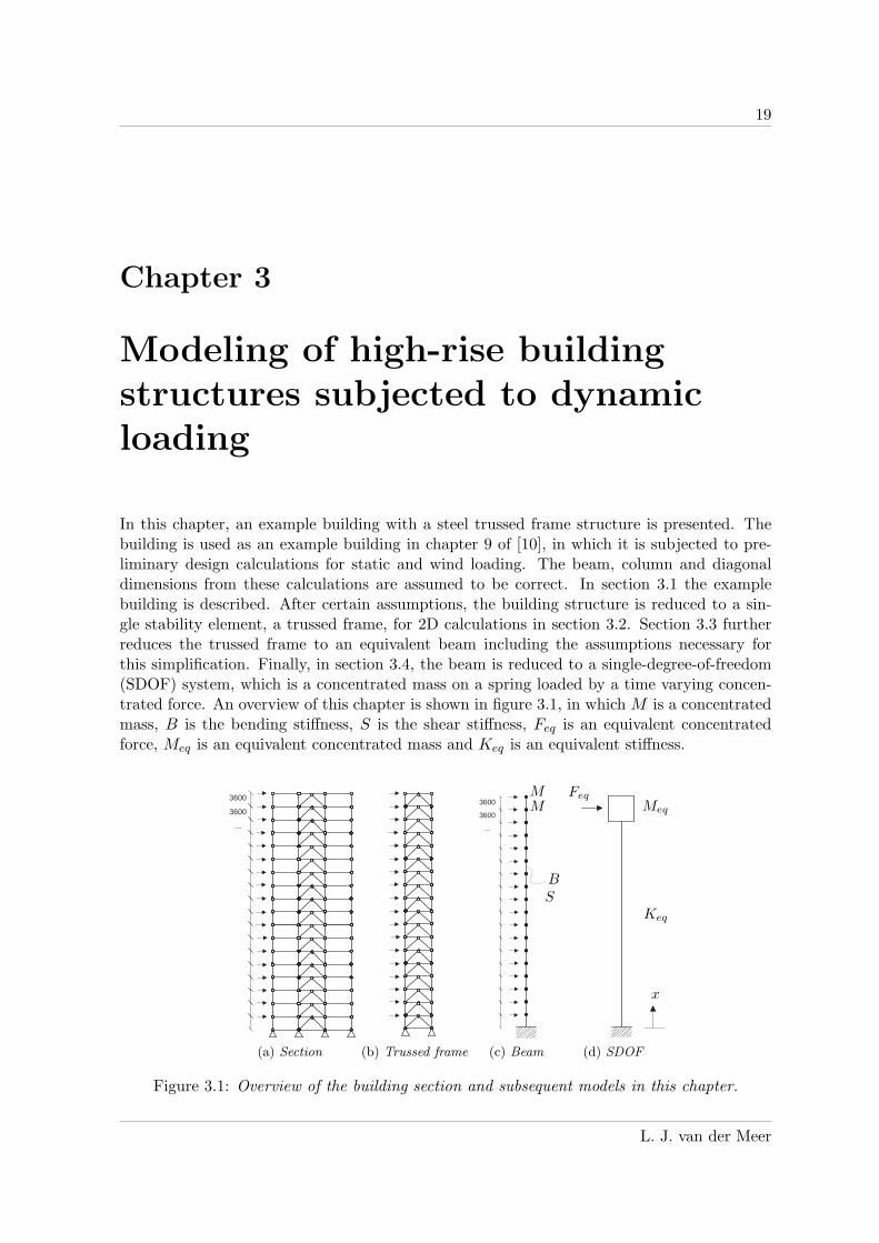
In this chapter, an example building with a steel trussed frame structure is presented. Thebuilding is used as an example building in chapter 9 of [10], in which it is subjected to pre-liminary design calculations for static and wind loading. The beam, column and diagonaldimensions from these calculations are assumed to be correct. In section 3.1 the examplebuilding is described. After certain assumptions, the building structure is reduced to a sin-gle stability element, a trussed frame, for 2D calculations in section 3.2. Section 3.3 furtherreduces the trussed frame to an equivalent beam including the assumptions necessary forthis simplification. Finally, in section 3.4, the beam is reduced to a single-degree-of-freedom(SDOF) system, which is a concentrated mass on a spring loaded by a time varying concen-trated force. An overview of this chapter is shown in figure 3.1, in which M is a concentratedmass, B is the bending stiffness, S is the shear stiffness, Feq is an equivalent concentratedforce, Meq is an equivalent concentrated mass and Keq is an equivalent stiffness.
3600
3600
...
(a) Section (b) Trussed frame
3600
3600
...
MM
BS
(c) Beam
Meq
Keq
Feq
x
(d) SDOF
Figure 3.1: Overview of the building section and subsequent models in this chapter.
L. J. van der Meer

20 Chapter 3: Modeling of high-rise building structures
3.1 Example of a realistic building structure
The building plan is shown in figure 3.2. The building dimensions are L × W × H =21.6m×50.4m×64.8m. The columns are placed on a grid of 7.2m×7.2m and the story heighth = 3.6m. Columns are HD400×744, diagonals are HF RHS300×12.5 and beams are HEB360.The stability is assured by 6 stability elements in the considered direction (the weak axis)and 4 in the other direction. The stability elements are K-shaped trussed frames. The rotarystiffness of the foundation of a single trussed frame is Cφ = 5.44 · 107 kNm. The steel qualityis S355. The mass carried by a single stability element is M = 2.06 · 106 kg.
7200 7200 ...
7200
...
modeled part
Figure 3.2: Building plan.
3.2 A stability element: the trussed frame
The following assumptions are made to convert the 3D building to a 2D trussed frame:
• The load distribution over the width W of the building is symmetric, so that there isno torsion.
• The floors are infinitely stiff in their plane.
• The total load is divided equally over the 6 trussed frames.
The distributed reflected overpressure pr(x, t) on the building is converted to a number ofconcentrated forces F (x, t) applied at floor levels. Since the total load is divided equally over6 trussed frames, the load F (x, t) applied at a floor level is approximately equal to
F (x, t) =pr(x, t)Wh
6(3.1)
in which W is the building width and h the story height. This expression is exact if the loaddistribution is linear. Otherwise it is an approximation.
One story of the trussed frame is shown in figure 3.3.
The trussed frame model was built in the finite element (FE) program ANSYS 11.0 usinglink elements with an axial stiffness (LINK1) and connected by hinges. The masses (MASS21)are lumped to the connections and the link elements are weightless. The rotary stiffness Cφ of
Dynamic response of high-rise building structures to blast loading

3.3 The equivalent beam 21
`
h d
F h`
F h`
EAb = ∞F
F2
F2
Figure 3.3: One story of the trussed frame.
the foundation (if taken into account) is converted to two translational springs (COMBIN14)with stiffness K between the columns of the trussed frame and the constraints. The columnscarrying the facade and the floors between these columns and the trussed frame are notmodeled (see figure 3.2), except for the part of the mass that is carried by the trussed frame.The trussed frame was modeled in ANSYS 11.0 to obtain the static deflection under windloading as well as the natural frequencies of the trussed frame, which is necessary to compareit to other models. The ANSYS 11.0 input file can be found in appendix B.
3.3 The equivalent beam
To reduce the trussed frame to an equivalent beam, the following assumptions are made:
• All connections are hinges.
• The bending stiffness B is completely determined by the axial stiffness EAc of thecolumns (figure 3.4a):
B =`2
2EAc (3.2)
• The shear stiffness S is completely determined by the axial stiffness EAd of the diagonals(figure 3.4b):
S =`2h
2d3EAd (3.3)
• The beams do not contribute to the shear stiffness, because they are assumed to beinfinitely stiff in their plane.
• The bending stiffness, shear stiffness and mass are constant over the height of thebeam. The fact that columns in actual buildings have smaller sections on upper storiesis neglected.
In the FE program ANSYS 11.0 the model was built with beam elements (BEAM3) andlumped masses (MASS21). The beam elements were configured to include shear deflection.The ANSYS 11.0 input file can be found in appendix B. The trussed frame and the equivalentbeam are compared by means of static analysis under wind loading and modal analysis in
L. J. van der Meer

22 Chapter 3: Modeling of high-rise building structures
(a) Bending
(b) Shear
Figure 3.4: Bending and shear in a trussed frame.
table 3.1. The static analysis results in a maximum displacement of the top. The modalanalysis gives the natural frequencies and mode shapes. Vertical degrees of freedom areconstrained. The first four natural frequencies are compared. Uniform loading is assumedand base rotation is ignored. The error percentage is defined as
EB − TF
TF· 100% (3.4)
in which EB is the value for the equivalent beam and TF the value for the trussed frame.The static deflection is overestimated (+9.5%) by the equivalent beam model and the firstnatural frequency is underestimated (−4.4%). This indicates that the equivalent beam modelis less stiff than the trussed frame, which is conservative. The higher natural frequencies areslightly overestimated. This inconsistency might be explained by the reduced accuracy of thefinite element solution for higher modes.
Analysis Result Trussed frame Eq. beam % ErrorStatic ym[mm] 50.99 55.83 +9.5Modal f1[Hz] 0.474 0.453 −4.4
f2[Hz] 1.934 1.918 −0.8f3[Hz] 4.016 4.017 +0.0f4[Hz] 6.012 6.031 +0.3
Table 3.1: Comparison of trussed frame and equivalent beam model using ANSYS 11.0.
3.4 The equivalent single degree of freedom system
In this section, the equivalent beam is reduced to a single-degree-of-freedom (SDOF) system,which is the most basic dynamic system that allows easy response calculations. A degree offreedom is a single translation or rotation of a concentrated mass. The beam has infinitedegrees of freedom if it is continuous (distributed mass) or it has the sum of degrees of
Dynamic response of high-rise building structures to blast loading

3.4 The equivalent single degree of freedom system 23
freedom of all lumped masses. If only the transverse deflection is considered, then the numberof lumped masses is equal to the number of degrees of freedom. A beam (and a structurein general) has as many natural frequencies and mode shapes as it has degrees of freedom.A mode shape or mode of vibration, is a particular shape that the structure adopts duringvibration at a specific natural frequency. The SDOF system vibrates only at the first naturalfrequency with a single shape, ideally the first mode shape. The following assumptions aremade for the reduction of the equivalent beam to the equivalent SDOF system:
• The dynamic response is determined completely by the first frequency and a singleresponse mode, ideally the first mode shape.
• The SDOF system is energy equivalent to the beam in this single response mode.
The second assumption is used to calculate the equivalent mass Meq and stiffness Keq of theSDOF system as well as the equivalent force Feq on the system. The lumped mass of theSDOF system can be made equivalent to the distributed mass of the beam, by assuming thatboth have the same kinetic energy. The spring stiffness of the SDOF system can be madeequivalent to the bending stiffness, shear stiffness and the rotary stiffness of the foundation ofthe beam, by assuming that both have the same strain energy. The concentrated force on theSDOF system can be made equivalent to the distributed force on the beam, by assuming thatthe work done by both forces is the same. The energy equivalence results in conversion factorsfor equivalent mass, stiffness and force in the SDOF system. For simplicity, it is assumedthat the beam is continuous, i.e. it has a uniform distributed mass, a distributed load anda constant bending and shear stiffness. In a real building, more mass is concentrated in thefloors than between the floors, so a real building is a continuous system with added mass atthe floor levels. To determine the conversion factors for mass, stiffness and force, considerthe continuous beam and equivalent SDOF system as shown in figure 3.5, in which H is thebuilding height, P (x) is the distributed load, ym is the maximum deflection at the top, ym isthe maximum velocity at the top (first time derivative of ym), y(x) is the shape function fortransverse deflection, B is the bending stiffness, S is the shear stiffness, Cφ is rotary stiffnessof the foundation, m is the distributed mass, Feq is the equivalent force, Meq is the equivalentmass and Keq is the equivalent stiffness.
The conversion factors can be found in literature [4] as the mass factor KM , resistancefactor KR and load factor KL. The mass factor is obtained from the kinetic energy equation,the resistance factor is obtained from the strain energy equation and the load factor is obtainedfrom the work done equation. The conversion factors are defined as follows:
KM =Ek;beam
Ek;sdof=
m2
x=H∫
x=0
y(x)2dx
M2 y(H)2
(3.5)
KR =Es;beam
Es;sdof=
12S
x=H∫
x=0
[v(x)]2dx + 12B
x=H∫
x=0
[µ(x)]2dx +Cφ
2
(
y(H)H
)2
12Ky(H)2
(3.6)
KL =Ew;beam
Ew;sdof=
x=H∫
x=0
y(x)P (x)dx
y(H)x=H∫
x=0
P (x)dx
(3.7)
L. J. van der Meer

24 Chapter 3: Modeling of high-rise building structures
P (x)
y(x)
H
ym,ym
Cφ
m
B
S
(a) Continuous beam
Meq
Keq
Feq
ym,ym
(b) Equivalent SDOF
Figure 3.5: Continuous beam vs equivalent SDOF system.
In these equations, x is the axial coordinate of the beam, which is H at the top and 0at the base (the x−coordinate can also be taken from top to base as long as this is doneconsequently). Ek, Es and Ew are the kinetic energy, strain energy and work done respectively.
Fortunately, it is not necessary to calculate KR. It can be proven that KR = KL. Inorder to prove this, a deflected shape function y(x) must be defined. This shape can be eitherthe first mode shape of the continuous beam or the deflected shape of the continuous beamunder the load P (x). In the first case, the natural frequency of the beam and equivalent SDOFsystem will match and the static deflection will be approximated. In the latter case, the staticdeflection of both systems will match and the first natural frequency will be approximated.Determining mode shapes for continuous beams is quite complicated, as can be seen in section5.2. Therefore, in this section the static deflected shape will be used as shape function. Beforemaking the SDOF system energy equivalent to the continuous beam, we reduce the continuousbeam to a non-equivalent SDOF system. This system has the following properties:
F =
H∫
0
P (x)dx = PmH
M = mH
K =F
y(H)y(H) =
F
K(3.8)
In equation (3.8), y(H) is the static deflection at the top due to the load P (x). The equivalentsystem should have the same static deflection y(H) at the top as the non-equivalent system,because both are defined to have the same static deflection at the top as the continuous beam.This results in:
y(H) =Feq
Keq=
KLF
KRK=
F
K→ KL = KR (3.9)
Dynamic response of high-rise building structures to blast loading
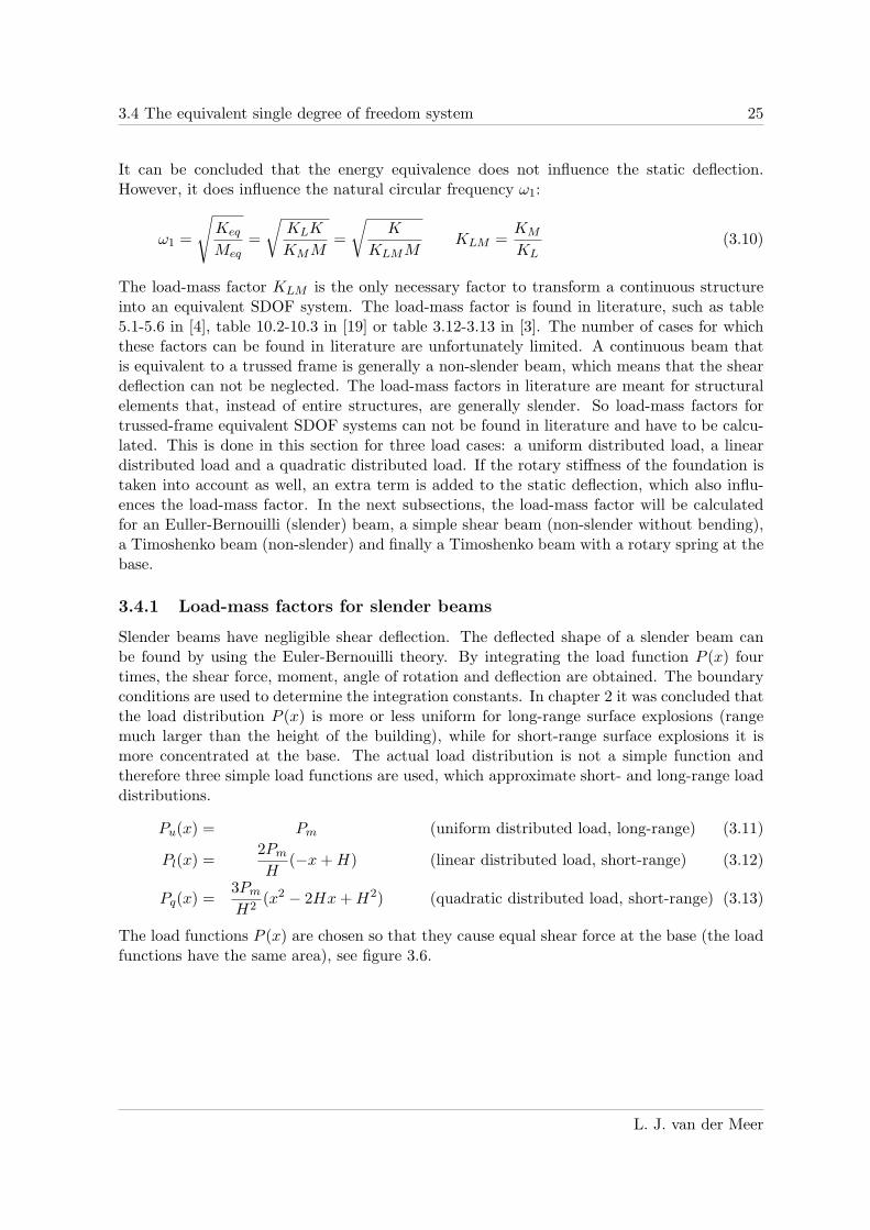
3.4 The equivalent single degree of freedom system 25
It can be concluded that the energy equivalence does not influence the static deflection.However, it does influence the natural circular frequency ω1:
ω1 =
√
Keq
Meq=
√
KLK
KMM=
√
K
KLMMKLM =
KM
KL(3.10)
The load-mass factor KLM is the only necessary factor to transform a continuous structureinto an equivalent SDOF system. The load-mass factor is found in literature, such as table5.1-5.6 in [4], table 10.2-10.3 in [19] or table 3.12-3.13 in [3]. The number of cases for whichthese factors can be found in literature are unfortunately limited. A continuous beam thatis equivalent to a trussed frame is generally a non-slender beam, which means that the sheardeflection can not be neglected. The load-mass factors in literature are meant for structuralelements that, instead of entire structures, are generally slender. So load-mass factors fortrussed-frame equivalent SDOF systems can not be found in literature and have to be calcu-lated. This is done in this section for three load cases: a uniform distributed load, a lineardistributed load and a quadratic distributed load. If the rotary stiffness of the foundation istaken into account as well, an extra term is added to the static deflection, which also influ-ences the load-mass factor. In the next subsections, the load-mass factor will be calculatedfor an Euller-Bernouilli (slender) beam, a simple shear beam (non-slender without bending),a Timoshenko beam (non-slender) and finally a Timoshenko beam with a rotary spring at thebase.
3.4.1 Load-mass factors for slender beams
Slender beams have negligible shear deflection. The deflected shape of a slender beam canbe found by using the Euler-Bernouilli theory. By integrating the load function P (x) fourtimes, the shear force, moment, angle of rotation and deflection are obtained. The boundaryconditions are used to determine the integration constants. In chapter 2 it was concluded thatthe load distribution P (x) is more or less uniform for long-range surface explosions (rangemuch larger than the height of the building), while for short-range surface explosions it ismore concentrated at the base. The actual load distribution is not a simple function andtherefore three simple load functions are used, which approximate short- and long-range loaddistributions.
Pu(x) = Pm (uniform distributed load, long-range) (3.11)
Pl(x) =2Pm
H(−x + H) (linear distributed load, short-range) (3.12)
Pq(x) =3Pm
H2(x2 − 2Hx + H2) (quadratic distributed load, short-range) (3.13)
The load functions P (x) are chosen so that they cause equal shear force at the base (the loadfunctions have the same area), see figure 3.6.
L. J. van der Meer

26 Chapter 3: Modeling of high-rise building structures
10 20 30 40 50 60
0.5
1
1.5
2
2.5
3
P (x)Pm
x
uniform
linear
quadratic
Figure 3.6: Three simple load distributions.
With the x−coordinate from base to top, the following boundary conditions have to besatisfied:
y(0) = 0 (3.14)
dy
dx(0) = 0 (3.15)
Bd2y
dx2(H) = 0 (3.16)
Bd3y
dx3(H) = 0 (3.17)
Respectively, deflection at the base is 0, angle of rotation at the base is 0, moment at the topis 0 and shear force at the top is 0. B is the bending stiffness EIz which can be ignored in theboundary condition since EIz 6= 0. Using these boundary conditions with the load functions,the shape functions are obtained:
yb;u(x) =Pm
B
[
x4
24− Hx3
6+
H2x2
4
]
yb;l(x) =Pm
BH
[
−x5
60+
Hx4
12− H2x3
6+
H3x2
6
]
yb;q(x) =Pm
BH2
[
x6
120− Hx5
20+
H2x4
8− H3x3
6+
H4x2
8
]
(3.18)
These are the deflected shapes for uniform load distribution yu, linear load distribution yl andquadratic load distribution yq. The functions are plotted in figure 3.7. These shape functionscan be used to calculate the mass factor (3.5) and load factor (3.7).
In (3.5), y is the variable instead of y, which is the time derivative of y. However, ifthe response of both the continuous beam and the equivalent SDOF system are written as aproduct of a spatial function and a time function, which is the same for both systems, thenthe ratio of the spatial functions will remain the same if the time function is differentiated:
Beam: f(x)f(t) f(x) = f(x)f(t)
SDOF: f(H)f(t) f(H) = f(H)f(t)
}
f(x)
f(H)=
f(x)
f(H)(3.19)
Dynamic response of high-rise building structures to blast loading

3.4 The equivalent single degree of freedom system 27
10 20 30 40 50 60
500000
1´106
1.5´106
2´106
y · BPm
x
uniform
linear
quadratic
Figure 3.7: Bending deflection for three load functions.
So the time functions or derivatives of time functions of both systems will cancel each otherwhen the load or mass factor is calculated.
In table 3.2 the load-mass factors and the natural frequencies ω1 for the three load func-
tions are shown. The exact value for the natural frequency ω1 = 3.516√
BmH4 [17]. Since
Load distribution KM KL KLM ω1 ·√
mH4
B
Uniform 104405 ≈ 0.26 2
5 = 0.40 5281 ≈ 0.64 3.53
Linear 125462 ≈ 0.27 5
21 ≈ 0.24 2522 ≈ 1.14 3.63
Quadratic 51182 ≈ 0.28 1
6 ≈ 0.17 15391 ≈ 1.68 3.78
Table 3.2: Load-mass factors for slender beams
the equivalent SDOF systems are optimized for static deflection, the natural frequencies areapproximated. The deflected shape under uniform loading gives the best approximation ofthe natural frequency, because this shape resembles most the first mode shape. Mode shapesand natural frequencies are determined by free vibration, so they are not influenced by theload.
3.4.2 Load-mass factors for simple shear beams
In this subsection, only shear deflection is considered and all other contributions (bending,base rotation) to deflection are ignored. Using the same method as in the previous subsection,
L. J. van der Meer
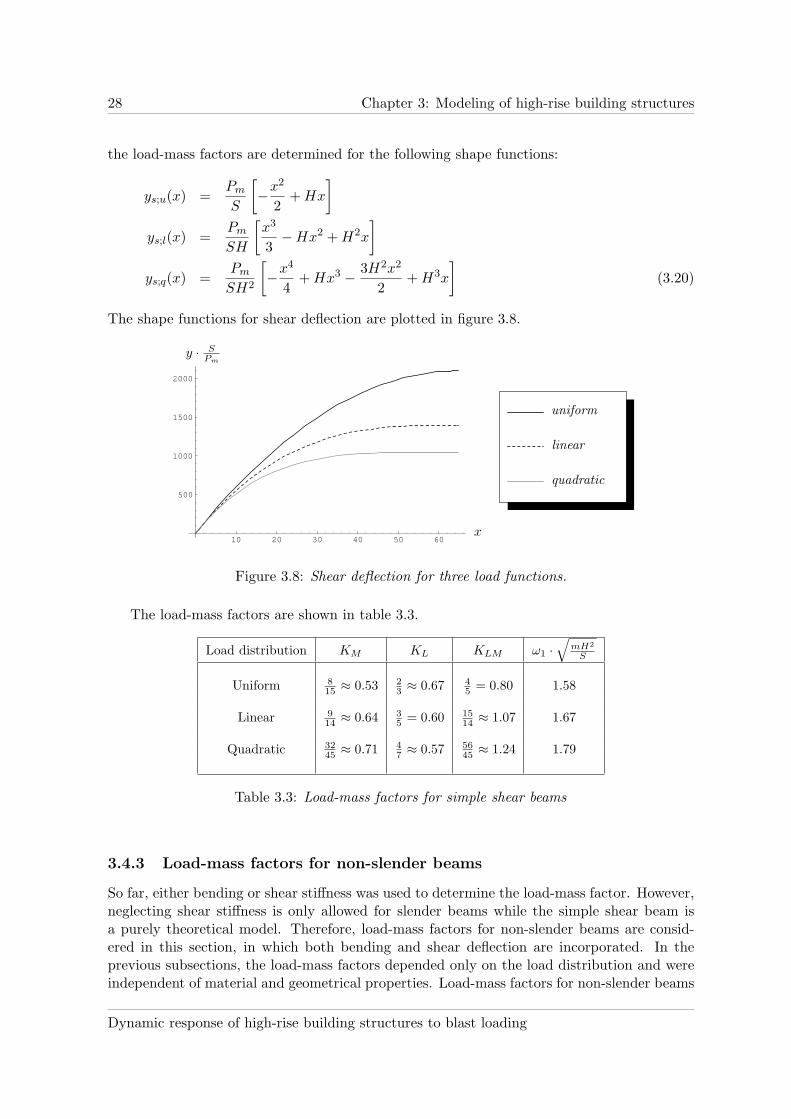
28 Chapter 3: Modeling of high-rise building structures
the load-mass factors are determined for the following shape functions:
ys;u(x) =Pm
S
[
−x2
2+ Hx
]
ys;l(x) =Pm
SH
[
x3
3− Hx2 + H2x
]
ys;q(x) =Pm
SH2
[
−x4
4+ Hx3 − 3H2x2
2+ H3x
]
(3.20)
The shape functions for shear deflection are plotted in figure 3.8.
10 20 30 40 50 60
500
1000
1500
2000
y · SPm
x
uniform
linear
quadratic
Figure 3.8: Shear deflection for three load functions.
The load-mass factors are shown in table 3.3.
Load distribution KM KL KLM ω1 ·√
mH2
S
Uniform 815 ≈ 0.53 2
3 ≈ 0.67 45 = 0.80 1.58
Linear 914 ≈ 0.64 3
5 = 0.60 1514 ≈ 1.07 1.67
Quadratic 3245 ≈ 0.71 4
7 ≈ 0.57 5645 ≈ 1.24 1.79
Table 3.3: Load-mass factors for simple shear beams
3.4.3 Load-mass factors for non-slender beams
So far, either bending or shear stiffness was used to determine the load-mass factor. However,neglecting shear stiffness is only allowed for slender beams while the simple shear beam isa purely theoretical model. Therefore, load-mass factors for non-slender beams are consid-ered in this section, in which both bending and shear deflection are incorporated. In theprevious subsections, the load-mass factors depended only on the load distribution and wereindependent of material and geometrical properties. Load-mass factors for non-slender beams
Dynamic response of high-rise building structures to blast loading
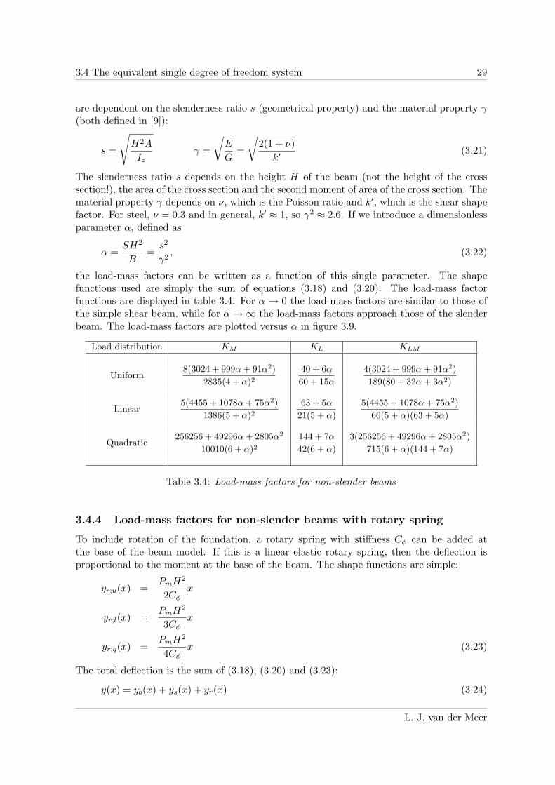
3.4 The equivalent single degree of freedom system 29
are dependent on the slenderness ratio s (geometrical property) and the material property γ(both defined in [9]):
s =
√
H2A
Izγ =
√
E
G=
√
2(1 + ν)
k′(3.21)
The slenderness ratio s depends on the height H of the beam (not the height of the crosssection!), the area of the cross section and the second moment of area of the cross section. Thematerial property γ depends on ν, which is the Poisson ratio and k′, which is the shear shapefactor. For steel, ν = 0.3 and in general, k′ ≈ 1, so γ2 ≈ 2.6. If we introduce a dimensionlessparameter α, defined as
α =SH2
B=
s2
γ2, (3.22)
the load-mass factors can be written as a function of this single parameter. The shapefunctions used are simply the sum of equations (3.18) and (3.20). The load-mass factorfunctions are displayed in table 3.4. For α → 0 the load-mass factors are similar to those ofthe simple shear beam, while for α → ∞ the load-mass factors approach those of the slenderbeam. The load-mass factors are plotted versus α in figure 3.9.
Load distribution KM KL KLM
Uniform8(3024 + 999α + 91α2)
2835(4 + α)240 + 6α
60 + 15α
4(3024 + 999α + 91α2)
189(80 + 32α + 3α2)
Linear5(4455 + 1078α + 75α2)
1386(5 + α)263 + 5α
21(5 + α)
5(4455 + 1078α + 75α2)
66(5 + α)(63 + 5α)
Quadratic256256 + 49296α + 2805α2
10010(6 + α)2144 + 7α
42(6 + α)
3(256256 + 49296α + 2805α2)
715(6 + α)(144 + 7α)
Table 3.4: Load-mass factors for non-slender beams
3.4.4 Load-mass factors for non-slender beams with rotary spring
To include rotation of the foundation, a rotary spring with stiffness Cφ can be added atthe base of the beam model. If this is a linear elastic rotary spring, then the deflection isproportional to the moment at the base of the beam. The shape functions are simple:
yr;u(x) =PmH2
2Cφx
yr;l(x) =PmH2
3Cφx
yr;q(x) =PmH2
4Cφx (3.23)
The total deflection is the sum of (3.18), (3.20) and (3.23):
y(x) = yb(x) + ys(x) + yr(x) (3.24)
L. J. van der Meer
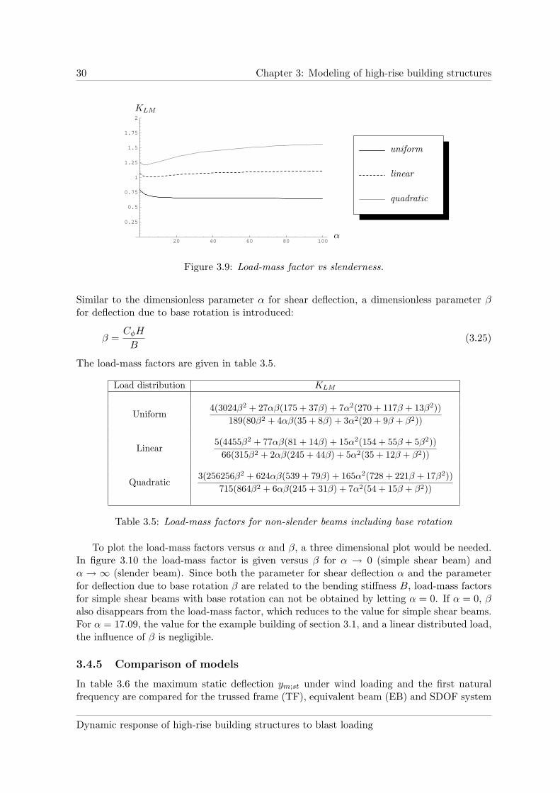
30 Chapter 3: Modeling of high-rise building structures
20 40 60 80 100
0.25
0.5
0.75
1
1.25
1.5
1.75
2
KLM
α
uniform
linear
quadratic
Figure 3.9: Load-mass factor vs slenderness.
Similar to the dimensionless parameter α for shear deflection, a dimensionless parameter βfor deflection due to base rotation is introduced:
β =CφH
B(3.25)
The load-mass factors are given in table 3.5.
Load distribution KLM
Uniform4(3024β2 + 27αβ(175 + 37β) + 7α2(270 + 117β + 13β2))
189(80β2 + 4αβ(35 + 8β) + 3α2(20 + 9β + β2))
Linear5(4455β2 + 77αβ(81 + 14β) + 15α2(154 + 55β + 5β2))
66(315β2 + 2αβ(245 + 44β) + 5α2(35 + 12β + β2))
Quadratic3(256256β2 + 624αβ(539 + 79β) + 165α2(728 + 221β + 17β2))
715(864β2 + 6αβ(245 + 31β) + 7α2(54 + 15β + β2))
Table 3.5: Load-mass factors for non-slender beams including base rotation
To plot the load-mass factors versus α and β, a three dimensional plot would be needed.In figure 3.10 the load-mass factor is given versus β for α → 0 (simple shear beam) andα → ∞ (slender beam). Since both the parameter for shear deflection α and the parameterfor deflection due to base rotation β are related to the bending stiffness B, load-mass factorsfor simple shear beams with base rotation can not be obtained by letting α = 0. If α = 0, βalso disappears from the load-mass factor, which reduces to the value for simple shear beams.For α = 17.09, the value for the example building of section 3.1, and a linear distributed load,the influence of β is negligible.
3.4.5 Comparison of models
In table 3.6 the maximum static deflection ym;st under wind loading and the first naturalfrequency are compared for the trussed frame (TF), equivalent beam (EB) and SDOF system
Dynamic response of high-rise building structures to blast loading
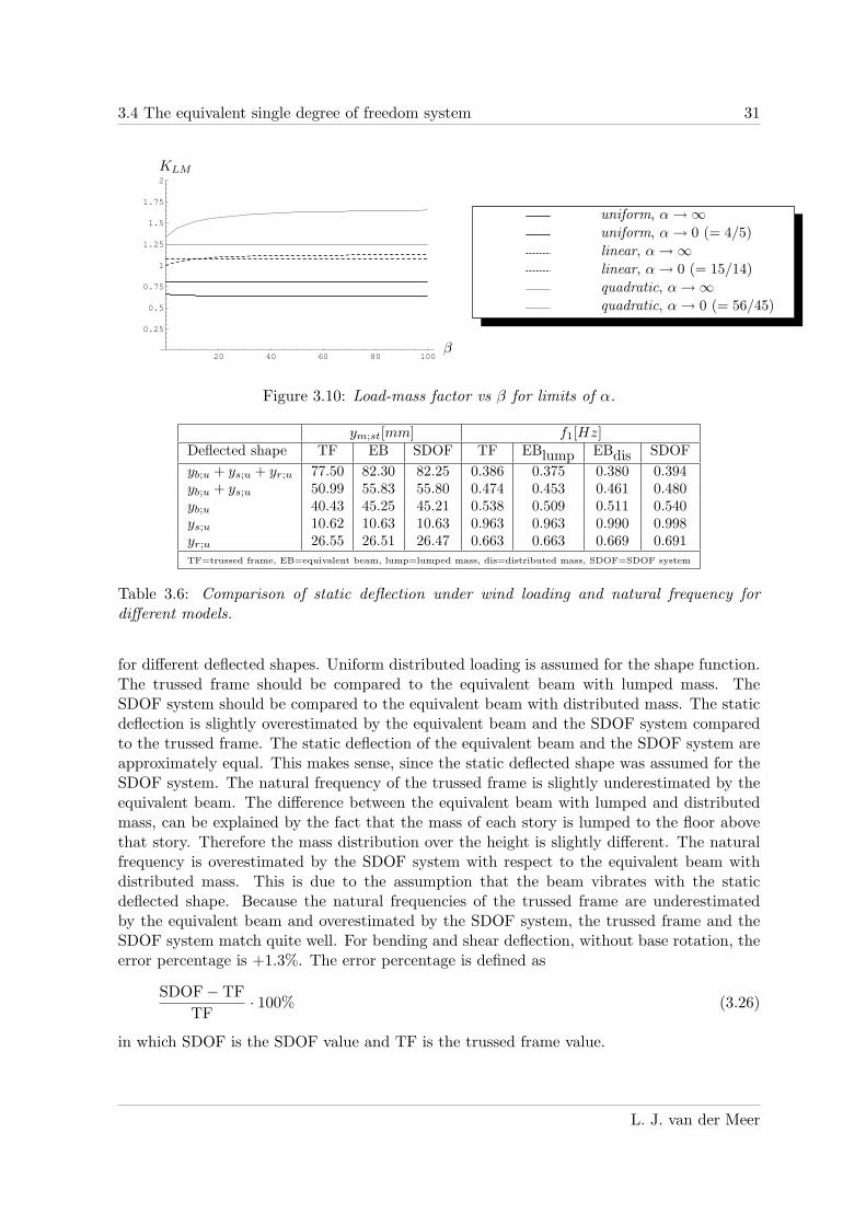
3.4 The equivalent single degree of freedom system 31
20 40 60 80 100
0.25
0.5
0.75
1
1.25
1.5
1.75
2
KLM
β
uniform, α → ∞uniform, α → 0 (= 4/5)
linear, α → ∞linear, α → 0 (= 15/14)
quadratic, α → ∞quadratic, α → 0 (= 56/45)
Figure 3.10: Load-mass factor vs β for limits of α.
ym;st[mm] f1[Hz]Deflected shape TF EB SDOF TF EBlump EBdis SDOF
yb;u + ys;u + yr;u 77.50 82.30 82.25 0.386 0.375 0.380 0.394yb;u + ys;u 50.99 55.83 55.80 0.474 0.453 0.461 0.480yb;u 40.43 45.25 45.21 0.538 0.509 0.511 0.540ys;u 10.62 10.63 10.63 0.963 0.963 0.990 0.998yr;u 26.55 26.51 26.47 0.663 0.663 0.669 0.691TF=trussed frame, EB=equivalent beam, lump=lumped mass, dis=distributed mass, SDOF=SDOF system
Table 3.6: Comparison of static deflection under wind loading and natural frequency fordifferent models.
for different deflected shapes. Uniform distributed loading is assumed for the shape function.The trussed frame should be compared to the equivalent beam with lumped mass. TheSDOF system should be compared to the equivalent beam with distributed mass. The staticdeflection is slightly overestimated by the equivalent beam and the SDOF system comparedto the trussed frame. The static deflection of the equivalent beam and the SDOF system areapproximately equal. This makes sense, since the static deflected shape was assumed for theSDOF system. The natural frequency of the trussed frame is slightly underestimated by theequivalent beam. The difference between the equivalent beam with lumped and distributedmass, can be explained by the fact that the mass of each story is lumped to the floor abovethat story. Therefore the mass distribution over the height is slightly different. The naturalfrequency is overestimated by the SDOF system with respect to the equivalent beam withdistributed mass. This is due to the assumption that the beam vibrates with the staticdeflected shape. Because the natural frequencies of the trussed frame are underestimatedby the equivalent beam and overestimated by the SDOF system, the trussed frame and theSDOF system match quite well. For bending and shear deflection, without base rotation, theerror percentage is +1.3%. The error percentage is defined as
SDOF − TF
TF· 100% (3.26)
in which SDOF is the SDOF value and TF is the trussed frame value.
L. J. van der Meer


33
Chapter 4
Dynamic response of a single degreeof freedom system to blast loading
In chapter 2 blast loading in general has been described as well as blast loading on buildingstructures in particular. An example building structure has been modeled in chapter 3. Inthis chapter, the focus is on the response of the single-degree-of-freedom (SDOF) system toblast loading. This SDOF system was described in section 3.4. The response of this systemto idealized blast loading is described in section 4.1.
In section 4.2 the dynamic load factor (DLF) is explained, which describes the ratio ofthe maximum dynamic response and the static response if the maximum dynamic load wereapplied as a static load. The DLF is dependent on the ratio of td and T1, the positive phaseduration of the blast and the natural period of vibration of the structure respectively. Thediagram of DLF versus the td/T1−ratio contains three regimes, namely an impulsive regime,a quasi-static regime and a dynamic transition region in between.
The pressure-impulse (p − i−) diagram, described in section 4.3, is a modification of theDLF −td/T1−diagram, which divides all possible combinations of pressure and impulse of theblast loading into two categories: either the blast exceeds the chosen damage criterium or itdoes not. The p−i−diagram is a powerful assessment tool, which is generally used to estimatethe maximum blast load capacity of structural elements, such as beams, slabs, plates, shellsetcetera. However, the method can also be applied to building structures as a whole, if onlythe overall response is considered. The overall response determines the internal forces in theelements. The response of building structure elements is only useful if the element is directlyexposed to the blast load. Yet structural stability elements, such as cores, stability walls or(trussed) frames, are often not even in the neighborhood of the building facade. Therefore,they should be assessed for overall response. Element response can be used to assess damageof facade elements or structural elements close to the facade. If any of these elements fail, thisfailure should be taken into account when assessing the overall response. In literature, theresistance of the building to progressive collapse due to failing structural elements is calledrobustness. However, this is not within the scope of this research.
In this chapter, response of a SDOF system is considered, which is a simplification ofan example building structure. In chapter 5 the example building structure is modeled as acontinuous beam with infinite-degrees-of-freedom (IDOF).
L. J. van der Meer
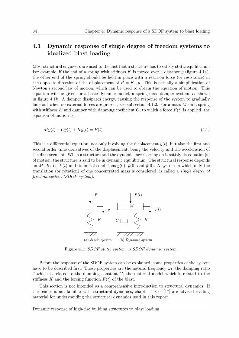
34 Chapter 4: Dynamic response of a SDOF system to blast loading
4.1 Dynamic response of single degree of freedom systems toidealized blast loading
Most structural engineers are used to the fact that a structure has to satisfy static equilibrium.For example, if the end of a spring with stiffness K is moved over a distance y (figure 4.1a),the other end of the spring should be held in place with a reaction force (or resistance) inthe opposite direction of the displacement of R = K · y. This is actually a simplification ofNewton’s second law of motion, which can be used to obtain the equation of motion. Thisequation will be given for a basic dynamic model, a spring-mass-damper system, as shownin figure 4.1b. A damper dissipates energy, causing the response of the system to graduallyfade out when no external forces are present, see subsection 4.1.2. For a mass M on a springwith stiffness K and damper with damping coefficient C, to which a force F (t) is applied, theequation of motion is:
My(t) + Cy(t) + Ky(t) = F (t) (4.1)
This is a differential equation, not only involving the displacement y(t), but also the first andsecond order time derivatives of the displacement, being the velocity and the acceleration ofthe displacement. When a structure and the dynamic forces acting on it satisfy its equation(s)of motion, the structure is said to be in dynamic equilibrium. The structural response dependson M , K, C, F (t) and its initial conditions y(0), y(0) and y(0). A system in which only thetranslation (or rotation) of one concentrated mass is considered, is called a single degree offreedom system (SDOF system).
K
F
y
(a) Static system
F (t)
M
K
y(t)
C
(b) Dynamic system
Figure 4.1: SDOF static system vs SDOF dynamic system.
Before the response of the SDOF system can be explained, some properties of the systemhave to be described first. These properties are the natural frequency ω1, the damping ratioζ which is related to the damping constant C, the material model which is related to thestiffness K and the forcing function F (t) of the blast.
This section is not intended as a comprehensive introduction to structural dynamics. Ifthe reader is not familiar with structural dynamics, chapter 1-8 of [17] are advised readingmaterial for understanding the structural dynamics used in this report.
Dynamic response of high-rise building structures to blast loading

4.1 Dynamic response of SDOF systems to idealized blast loading 35
4.1.1 Natural frequency of vibration
The SDOF system as shown in figure 4.1b has a natural frequency of vibration, equal to:
ω1 =
√
K
M
[
rad
s
]
(4.2)
With some sort of damping with damping constant C, the damped ’frequency’ of vibrationis:
ω1;ζ =
√
K
M−
(
C
2M
)2 [
rad
s
]
(4.3)
These frequencies are circular frequencies in rad/s. The natural frequency f1 = ω1/(2π). Thenatural period T1 = 1/f1 = 2π/ω1.
4.1.2 Damping
Without damping, the resulting vibrations of an applied force that is no longer present wouldgo on forever. Damping is the dissipation of energy of the system, which causes the vibrationsto gradually fade-out if the force is no longer present. The energy which is lost is convertedto heat or sound. Different types of damping can be present in a system simultaneously:
• Viscous damping is the damping caused by resistance of a fluid medium such as forexample air, gas or water.
• Dry friction damping is the damping caused by friction between surfaces.
• Material damping is the damping caused by cyclic plastic deformation of materials.
When a building vibrates, viscous damping is caused by the resistance of the surrounding airand material damping occurs when the elastic limits of structural elements are exceeded. Dryfriction damping can occur during earthquakes between the building foundation and the soil.It is difficult to estimate the damping ratio of a vibrating building and it is conservative toignore damping. However, ignoring damping is not always allowed. In general, for structuresloaded with periodic forces, damping can not be ignored, because damping has a significantinfluence on the response to periodic forces near resonance. Without damping, response atresonance is infinite.
For a SDOF system, the critical damping coefficient is Cc = 2Mω1, which is the dampingcoefficient at which so much energy is dissipated in damping, that the mass does not oscillateat all but only returns to its equilibrium position. The damping ratio is defined as:
ζ =C
Cc(4.4)
Therefore, the natural circular frequency of a damped system can be written as:
ω1;ζ =√
1 − ζ2ω1 (4.5)
For small amounts of damping the damped and undamped frequency are almost equal, sothat the use of the undamped frequency is permitted.
L. J. van der Meer

36 Chapter 4: Dynamic response of a SDOF system to blast loading
In this chapter, damping is neglected, because the maximum response to a blast load, isalways the first maximum of the response after the maximum of the blast load. The effect ofdamping increases with the number of oscillations. The first maximum of response is usuallywithin the first oscillation, where the effect of damping is still small. Moreover, dampingalways decreases the maximum response, so neglecting damping is always conservative.
4.1.3 Material model
In differential equation 4.1 all terms are linear functions of y, y or y. If one or more of theterms are non-linear functions of y or its derivatives, the vibration is called non-linear. Exam-ples of nonlinearity are a pendulum swinging with large amplitudes (geometric nonlinearity),a nonlinear spring (material nonlinearity), nonlinear damping or a variable mass system. Ma-terial nonlinearity is likely to occur, because structural materials such as steel and concretebehave elastic-plastic. Because buildings are generally not designed for blast loads, stressesabove the yield limit might occur. In this report, only the material steel is considered, whichbehaves linear-elastic and has a critical resistance related to the yield stress. Therefore theinfluence of ductility on the response is not investigated. Ductility is the ratio of the criticalplastic deformation yc;p and the critical elastic deformation yc;e, see figure 4.2. Ignoring theinfluence of ductility in combination with a critical resistance related to the yield stress isconservative, because it ensures that the structure is loaded in the elastic range even thoughthere is always some additional plastic capacity.
R(y)
y
Rc = Kyc
yc;e yc;p
Figure 4.2: Linear-elastic (continuous line) vs elastic-plastic (dashed line) material model.
4.1.4 Forcing function
How the response of a SDOF system is determined, depends on the forcing function F (t).When the forcing function is an harmonic function, the response will also be an harmonicfunction and is relatively easy to determine. In case of a periodic non-harmonic function,the function can be written as a sum of harmonic functions using Fourier series expansion.When the function is non-periodic, other methods are available to determine the response,see subsection 4.1.5. To determine the response analytically, blast pressure-time profiles suchas in figure 2.3 have to be given analytically. Since the actual blast pressure-time variation is
Dynamic response of high-rise building structures to blast loading
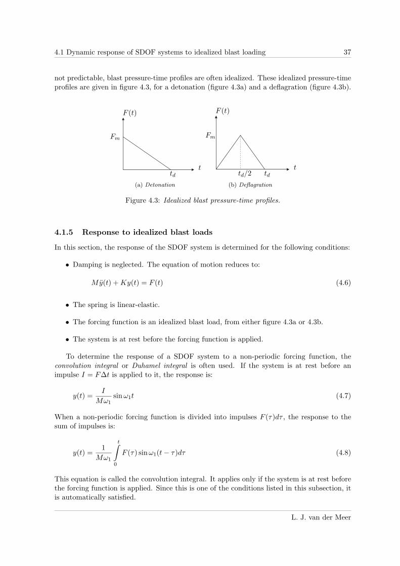
4.1 Dynamic response of SDOF systems to idealized blast loading 37
not predictable, blast pressure-time profiles are often idealized. These idealized pressure-timeprofiles are given in figure 4.3, for a detonation (figure 4.3a) and a deflagration (figure 4.3b).
t
F (t)
Fm
td
(a) Detonation
t
F (t)
Fm
tdtd/2
(b) Deflagration
Figure 4.3: Idealized blast pressure-time profiles.
4.1.5 Response to idealized blast loads
In this section, the response of the SDOF system is determined for the following conditions:
• Damping is neglected. The equation of motion reduces to:
My(t) + Ky(t) = F (t) (4.6)
• The spring is linear-elastic.
• The forcing function is an idealized blast load, from either figure 4.3a or 4.3b.
• The system is at rest before the forcing function is applied.
To determine the response of a SDOF system to a non-periodic forcing function, theconvolution integral or Duhamel integral is often used. If the system is at rest before animpulse I = F∆t is applied to it, the response is:
y(t) =I
Mω1sinω1t (4.7)
When a non-periodic forcing function is divided into impulses F (τ)dτ , the response to thesum of impulses is:
y(t) =1
Mω1
t∫
0
F (τ) sin ω1(t − τ)dτ (4.8)
This equation is called the convolution integral. It applies only if the system is at rest beforethe forcing function is applied. Since this is one of the conditions listed in this subsection, itis automatically satisfied.
L. J. van der Meer

38 Chapter 4: Dynamic response of a SDOF system to blast loading
It is convenient to write response in dimensionless form. Therefore, the following expres-sions are defined (as in reference [13]):
Fm =Fm
Rctd = ω1td I = Fm
∫ td
0F (t)dt
y =y
yc
˙y =y
ω1yct = ω1t F =
F
Fm(4.9)
In which Fm is the non-dimensional maximum force, Fm is the maximum force, Rc is thecritical resistance, td is similar to the ratio td/T1 but in radians, ω1 is the natural circularfrequency of the structure, I is the non-dimensional total impulse, y is the response as afraction of the critical response and F is the non-dimensional force. The parameters areexplained graphically in figure 4.4.
R(y)
Rc
ycy
(a) Resistance
Fm
I
t
F (t)
td
(b) Force
F (t)
1
tdt
I/Fm
(c) Dimensionless
Figure 4.4: Parameters for response in dimensionless form.
Response to an idealized detonation
Using the dimensionless parameters defined in subsection 4.1.5, the force function for anidealized detonation (figure 4.3a) is:
F (t, td) =
(
1 − t
td
)
[u(t) − u(t − td)] (4.10)
where u is a unit-step function. The response to this force function using the Convolutionintegral is:
y(t, td) = Fm
t∫
0
F (τ) sin(t− τ)dτ = Fm
− t
td+ 1 − cos t +
sin t
tdif t ≤ td
− cos t +sin t
td− sin(t − td)
tdif t > td
(4.11)
Response for different td is given in figure 4.5. For completeness the response is also given ifdamping is present (ζ = 0.10). The dimensionless blast duration td is equal to the ratio td/T1
multiplied by 2π. If this ratio becomes greater, more oscillations occur during the presenceof the forcing function. It is also observed that for a damping percentage of 10%, the timeof maximum response is barely influenced and the maximum response itself is slightly lower.This agrees with the assumption that ignoring damping is conservative.
Dynamic response of high-rise building structures to blast loading

4.2 Time of maximum deflection and the dynamic load factor 39
1 2 3 4
-2
-1.5
-1
-0.5
0.5
1
1.5
2
t
y
Fm
,F
(a) td = 2, undamped
1 2 3 4
-2
-1.5
-1
-0.5
0.5
1
1.5
2
t
y
Fm
,F
(b) td = 2, damped
10 20 30 40
-2
-1.5
-1
-0.5
0.5
1
1.5
2
t
y
Fm
,F
(c) td = 20, undamped
10 20 30 40
-2
-1.5
-1
-0.5
0.5
1
1.5
2
t
y
Fm
,F
(d) td = 20, damped
Figure 4.5: SDOF response to idealized detonation for different td and with and withoutdamping.
Response to an idealized deflagration
Using the dimensionless parameters defined in subsection 4.1.5, the force function for anidealized detonation (figure 4.3b) is:
F (t, td) =2t
td
[
u(t) − u
(
t − td2
)]
+ 2
(
1 − t
td
)[
u
(
t − td2
)
− u(t − td)
]
(4.12)
To which the response is:
y(t, td) =2t
td−2 sin t
td+u
(
t − td2
)
−4t
td+ 2 +
4 sin(
t − td2
)
td
+u(t−td)
[
2t
td− 2 − 2 sin(t − td)
td
]
(4.13)
Again u is a unit-step function. Response for different td is given in figure 4.6. For complete-ness the response is also given if damping is present (ζ = 0.10). From comparison of figures4.5 and 4.6 it can be concluded that a detonation causes higher response than deflagration forlarge td. Another important conclusion is the fact that the maximum response always occursafter the maximum force. For a detonation this is trivial but it is also true for a deflagration.For small values of td it does not seem to matter significantly whether the blast is a detonationor deflagration.
4.2 Time of maximum deflection and the dynamic load factor
As mentioned before, only the first maximum of the response that occurs after the maximumload is of interest, when the resistance to blast loading is to be determined. In figures 4.5 and
L. J. van der Meer
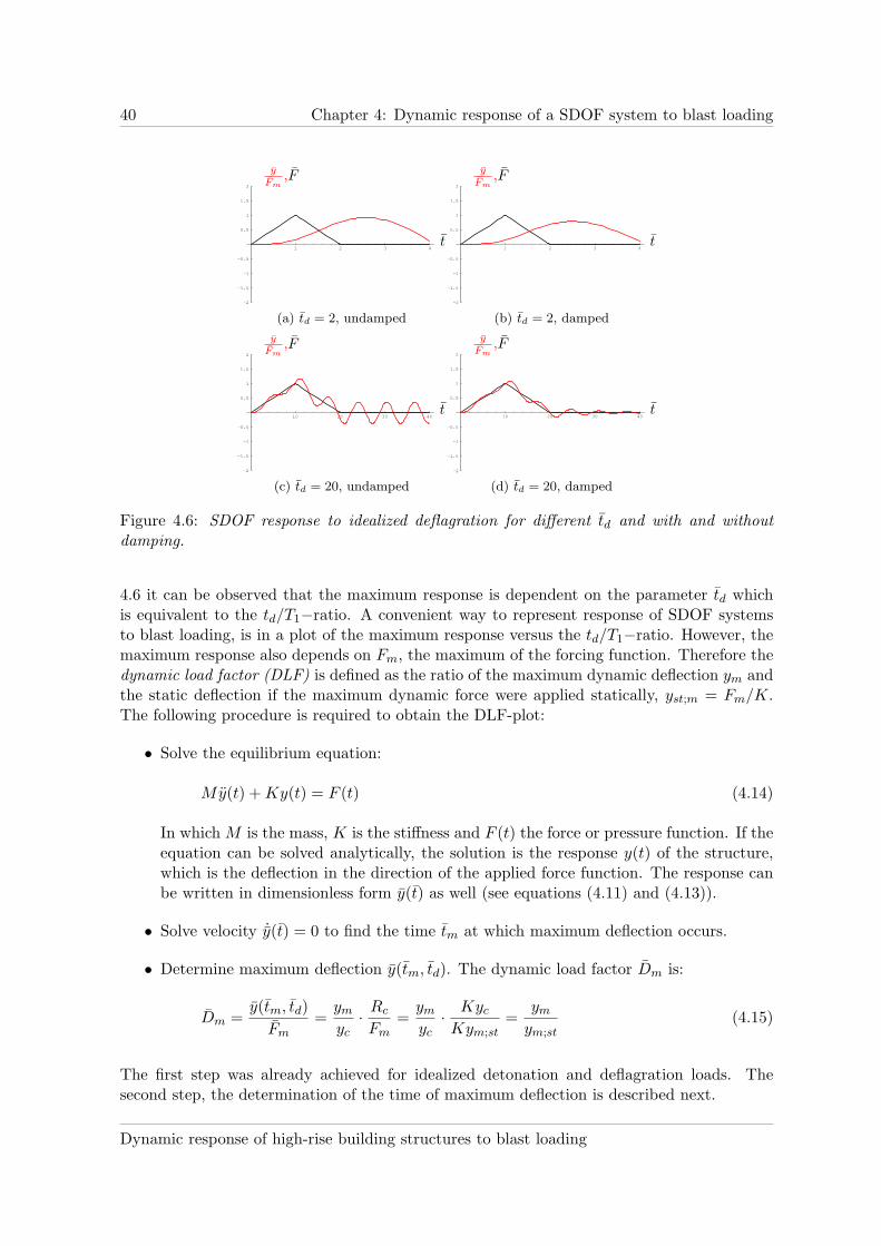
40 Chapter 4: Dynamic response of a SDOF system to blast loading
1 2 3 4
-2
-1.5
-1
-0.5
0.5
1
1.5
2
t
y
Fm
,F
(a) td = 2, undamped
1 2 3 4
-2
-1.5
-1
-0.5
0.5
1
1.5
2
t
y
Fm
,F
(b) td = 2, damped
10 20 30 40
-2
-1.5
-1
-0.5
0.5
1
1.5
2
t
y
Fm
,F
(c) td = 20, undamped
10 20 30 40
-2
-1.5
-1
-0.5
0.5
1
1.5
2
t
y
Fm
,F
(d) td = 20, damped
Figure 4.6: SDOF response to idealized deflagration for different td and with and withoutdamping.
4.6 it can be observed that the maximum response is dependent on the parameter td whichis equivalent to the td/T1−ratio. A convenient way to represent response of SDOF systemsto blast loading, is in a plot of the maximum response versus the td/T1−ratio. However, themaximum response also depends on Fm, the maximum of the forcing function. Therefore thedynamic load factor (DLF) is defined as the ratio of the maximum dynamic deflection ym andthe static deflection if the maximum dynamic force were applied statically, yst;m = Fm/K.The following procedure is required to obtain the DLF-plot:
• Solve the equilibrium equation:
My(t) + Ky(t) = F (t) (4.14)
In which M is the mass, K is the stiffness and F (t) the force or pressure function. If theequation can be solved analytically, the solution is the response y(t) of the structure,which is the deflection in the direction of the applied force function. The response canbe written in dimensionless form y(t) as well (see equations (4.11) and (4.13)).
• Solve velocity ˙y(t) = 0 to find the time tm at which maximum deflection occurs.
• Determine maximum deflection y(tm, td). The dynamic load factor Dm is:
Dm =y(tm, td)
Fm=
ym
yc· Rc
Fm=
ym
yc· Kyc
Kym;st=
ym
ym;st(4.15)
The first step was already achieved for idealized detonation and deflagration loads. Thesecond step, the determination of the time of maximum deflection is described next.
Dynamic response of high-rise building structures to blast loading

4.2 Time of maximum deflection and the dynamic load factor 41
4.2.1 Time of maximum deflection
The time of maximum deflection is found by equating the first time derivative of the responseto zero and solving for t. The first solution for t that occurs after the maximum of the blastload is the time of maximum deflection tm. Because the response is different for t ≤ td andt > td, there are also two values of tm, namely one for tm ≤ td and one for tm > td. The firstsolution is valid when the maximum response occurs during the blast and the latter is validwhen the maximum response occurs after the blast load has ended.
Time of maximum deflection for an idealized detonation
The time of maximum deflection for an idealized detonation is obtained by differentiating(4.11) to t, equating the result to zero and solving for t. The result is:
tm =
arccos
[
(cos td − 1)(td − sin td)√
(cos td − 1)2√
2 + (td)2 − 2 cos td − 2td − 2td sin td
]
if tm > td
2 arctan td if tm ≤ td
(4.16)
Maximum deflection occurs either during or after the blast. The shifting point is at tm =td = 2.33112.
Time of maximum deflection for an idealized deflagration
The time of maximum deflection for an idealized detonation is obtained by differentiating(4.13) to t, equating the result to zero and solving for t. The result is:
tm =
2 arctan
1 + tantd4
1 − tantd4
if tm ≥ td
2 arctan
−2 tantd4−√
2
√
tan
(
td4
)2
+ tan
(
td4
)4
−1 + tan
(
td4
)2
+ k2π ≥ td2
if tm < td
(4.17)
in which k is an integer. The maximum of the blast is at td/2, therefore the maximumresponse always occurs after or at this time. The shifting point is at tm = td = π.
In figure 4.7, the time of maximum deflection is shown versus the duration of the blast.For convenience, the dimensionless parameters have been converted to ratios of dimensionalparameters. Figure 4.7a shows the ratio of tm and T1 versus the ratio of td and T1. In figure4.7b, tm/T1 is changed to tm/td because this ratio shows immediately whether the maximumresponse occurs during (tm/td < 1) or after (tm/td > 1) the blast.
L. J. van der Meer
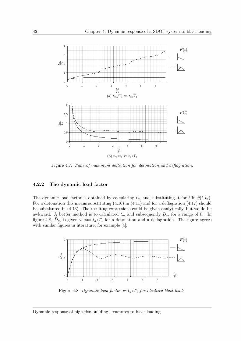
42 Chapter 4: Dynamic response of a SDOF system to blast loading
0
1
2
3
4
0 1 2 3 4 5 6
t m T1
td
T1
F (t)
(a) tm/T1 vs td/T1
0
0.5
1
1.5
2
0 1 2 3 4 5 6 td
T1
t m t d
F (t)
(b) tm/td vs td/T1
Figure 4.7: Time of maximum deflection for detonation and deflagration.
4.2.2 The dynamic load factor
The dynamic load factor is obtained by calculating tm and substituting it for t in y(t, td).For a detonation this means substituting (4.16) in (4.11) and for a deflagration (4.17) shouldbe substituted in (4.13). The resulting expressions could be given analytically, but would beawkward. A better method is to calculated tm and subsequently Dm for a range of td. Infigure 4.8, Dm is given versus td/T1 for a detonation and a deflagration. The figure agreeswith similar figures in literature, for example [4].
0
1
2
0 1 2 3 4 5 6
F (t)
td
T1
Dm
Figure 4.8: Dynamic load factor vs td/T1 for idealized blast loads.
Dynamic response of high-rise building structures to blast loading

4.2 Time of maximum deflection and the dynamic load factor 43
4.2.3 Limits of the dynamic load factor
To interpret the Dm − td/T1−diagram, it is instructive to look at the limits of Dm whentd/T1 → 0 and td/T1 → ∞. In the first case, the duration of the blast is very short comparedto the natural period of the SDOF system. An impulse has exactly this property, so toevaluate this limit, Dm is determined for impulse response. Impulse response is displayed in(4.7). Written in dimensionless variables:
y(t) = I sin t → D(t) =y(tm)
Fm=
td2
sin t → Dm =td2
=πtdT1
(4.18)
Apparently the diagram contains an impulsive asymptote for which Dm can be determinedwith πtd/T1. Notice that Dm for the impulsive asymptote is independent of the pressure-timeprofile and only depends on the ratio td/T1.
The other limit, where td/T1 → ∞, the detonation blast load becomes a step force whereasthe deflagration blast load becomes a linear rising load. The response D(t) to a step forcecan be determined with, for example, the convolution integral:
F (t) = 1 → D(t) =
t∫
0
sin(t − τ)dτ = 1 − cos t → Dm = 2 (4.19)
Thus the maximum dynamic load factor for an idealized detonation is equal to 2. Moreover,the maximum dynamic load factor for all decaying blast loads is equal to 2. However, someblast loads such as the idealized deflagration have an initial rise and reach their maximumafter some time. The maximum force of the idealized deflagration is reached at td/2.
F (t) = 2t
td→ D(t) =
t∫
0
2t
tdsin(t − τ)dτ =
2t − 2 sin t
td(4.20)
At first sight this expression does not seem to give the maximum dynamic load factor foran idealized deflagration. Yet, when td/T1 → ∞, tm = td/2, because the natural periodT1 becomes infinitely small compared to td. Since the response has a maximum in everyoscillation, it also has a maximum in the oscillation where t = td/2. Another requirement forthe time of maximum deflection is tm = k2π with k = 1, 2, . . ., because otherwise D(t) doesnot have a maximum.
tm = k2π =td2
→ Dm =2tm − 2 sin tm
td=
tdtd
− 2 sin(k2π) = 1 − 0 = 1 (4.21)
It can be concluded that the Dm−td/T1−diagram of an idealized detonation and deflagrationhave horizontal asymptotes at Dm = 2 and 1 respectively. These asymptotes are referred toin literature as quasi-static asymptotes.
The limits of tm follow simply from the expressions D(t) in equation (4.18) and (4.19).The impulse response is a sine function. A sine function (with phase=0) has its first maximumat T1/4. So:
td/T1 → 0 tm/T1 → 1/4 (4.22)
L. J. van der Meer
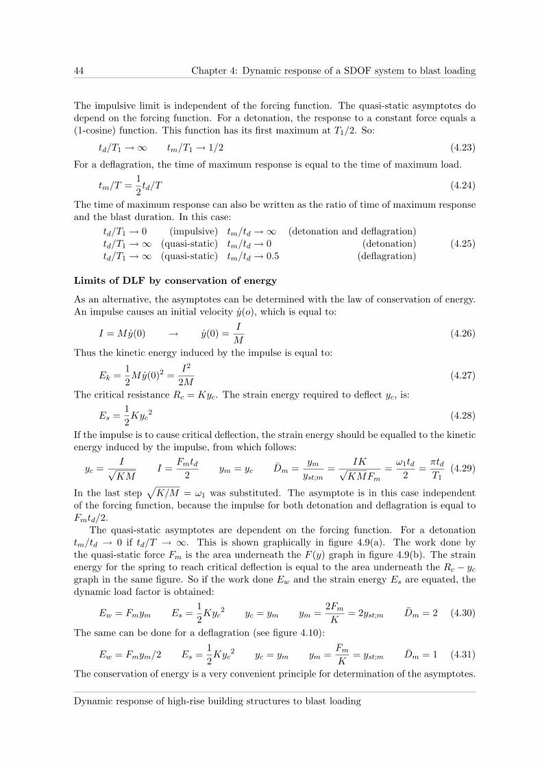
44 Chapter 4: Dynamic response of a SDOF system to blast loading
The impulsive limit is independent of the forcing function. The quasi-static asymptotes dodepend on the forcing function. For a detonation, the response to a constant force equals a(1-cosine) function. This function has its first maximum at T1/2. So:
td/T1 → ∞ tm/T1 → 1/2 (4.23)
For a deflagration, the time of maximum response is equal to the time of maximum load.
tm/T =1
2td/T (4.24)
The time of maximum response can also be written as the ratio of time of maximum responseand the blast duration. In this case:
td/T1 → 0 (impulsive) tm/td → ∞ (detonation and deflagration)td/T1 → ∞ (quasi-static) tm/td → 0 (detonation)td/T1 → ∞ (quasi-static) tm/td → 0.5 (deflagration)
(4.25)
Limits of DLF by conservation of energy
As an alternative, the asymptotes can be determined with the law of conservation of energy.An impulse causes an initial velocity y(o), which is equal to:
I = My(0) → y(0) =I
M(4.26)
Thus the kinetic energy induced by the impulse is equal to:
Ek =1
2My(0)2 =
I2
2M(4.27)
The critical resistance Rc = Kyc. The strain energy required to deflect yc, is:
Es =1
2Kyc
2 (4.28)
If the impulse is to cause critical deflection, the strain energy should be equalled to the kineticenergy induced by the impulse, from which follows:
yc =I√KM
I =Fmtd
2ym = yc Dm =
ym
yst;m=
IK√KMFm
=ω1td
2=
πtdT1
(4.29)
In the last step√
K/M = ω1 was substituted. The asymptote is in this case independentof the forcing function, because the impulse for both detonation and deflagration is equal toFmtd/2.
The quasi-static asymptotes are dependent on the forcing function. For a detonationtm/td → 0 if td/T → ∞. This is shown graphically in figure 4.9(a). The work done bythe quasi-static force Fm is the area underneath the F (y) graph in figure 4.9(b). The strainenergy for the spring to reach critical deflection is equal to the area underneath the Rc − yc
graph in the same figure. So if the work done Ew and the strain energy Es are equated, thedynamic load factor is obtained:
Ew = Fmym Es =1
2Kyc
2 yc = ym ym =2Fm
K= 2yst;m Dm = 2 (4.30)
The same can be done for a deflagration (see figure 4.10):
Ew = Fmym/2 Es =1
2Kyc
2 yc = ym ym =Fm
K= yst;m Dm = 1 (4.31)
The conservation of energy is a very convenient principle for determination of the asymptotes.
Dynamic response of high-rise building structures to blast loading

4.3 The pressure-impulse diagram 45
F (t)
RcRc
FmFm
F (y)
tm
td
t
(a) (b)
ym yc y
Figure 4.9: Quasi-static force-time and force-displacement for detonation.
F (t)
RcRc
FmFm
F (y)
tm td t
(a) (b)
ym yc y
Figure 4.10: Quasi-static force-time and force-displacement for deflagration.
4.3 The pressure-impulse diagram
First of all, pressure-impulse diagram is a misleading name, because it is used in literature forforce-impulse diagrams as well. In this report, this tradition is followed, but the axes labelsalways make clear what diagram it is. p is pressure (force per square meter), F is force, Pis force per meter. Similarly, i is the impulse from pressure, I is the impulse from force andJ is the impulse from force per meter. Because SDOF systems are loaded by a force, theconstructed diagrams are F − I−diagrams.
The pressure-impulse diagram is a modification of the Dm − td/T1−diagram. Instead ofDm and td, the x− and y−axis are labeled with Fm and I. This results in a modification ofthe asymptotes. The impulsive asymptote is modified as follows:
Dm =td2
Fm =1
Dm=
2
tdI =
Fmtd2
= 1 (4.32)
So instead of linear, the impulsive asymptote is now vertical. The quasi-static asymptotesare simply the reciprocal values of the asymptotes in the DLF-diagram.
td/T1 → ∞ I =πFmtd
T1→ ∞ Dm → 2 Fm → 1
2 (detonation)
td/T1 → ∞ I =πFmtd
T1→ ∞ Dm → 1 Fm → 1 (deflagration)
(4.33)
L. J. van der Meer

46 Chapter 4: Dynamic response of a SDOF system to blast loading
The pressure-impulse diagram is shown in figure 4.12. Is was determined in Excel. Alterna-tively, p − i−diagrams can be determined in Matlab, see appendix A. It agrees with similardiagrams in literature, for example [19].
The pressure-impulse diagram can be divided in three distinct regimes:
• The impulsive regime: the response is determined by the impulse. The shape of theblast load pressure-time profile does not have any influence on the response. Transientanalysis is not necessary.
• The quasi-static regime: the response is determined by the load, which is applied asa step force (detonation) or as a linear rising force (deflagration). The shape of theblast-load pressure-time profile does not have influence on the response, except for thedifference between decaying and linear rising forces. Transient analysis is not necessary.
• The dynamic regime: the response is determined by load, impulse and shape of theblast load pressure-time profile. The response can not be approximated by one of theasymptotes. The time of maximum response tm and the duration of the blast td areapproximately equal. Transient analysis is necessary.
A schematic pressure-impulse diagram is shown in figure 4.11, where the regimes and therelated force and resistance functions are shown. Only for the relatively small dynamic regime,dynamic response calculations are necessary. The diagram is constructed by using the damagecriterium y = ym/yc = 1. If the damage criterium is intensified, the asymptotes in thediagram move towards the axes. When the damage criterium is loosened, the asymptotes inthe diagram move away from the axes. The combinations of force and impulse, which areexactly on the line in the diagram, satisfy the damage criterium exactly. Combinations belowor left of the diagram do not cause damage whereas combinations to the right or above thediagram exceed the damage criterium. The damage criterium or critical resistance Rc can beformulated for any type of failure. Often different types of failure can occur in a structure.In that case, the failure that occurs at the lowest resistance governs the critical resistance.Or alternatively, p − i−diagrams for several failure types can be plotted together.
4.3.1 Pressure-impulse diagrams in literature
The pressure-impulse diagrams in this report were created by using the methods and di-mensionless variables of [13] and [14], which describe the construction of pressure-impulsediagrams for elastic and elastic-plastic material behavior respectively for three different pulseloading shapes: rectangular, linear decaying (triangular) and exponential decaying. One ofthe early investigators of the pressure-impulse diagram describe several aspects of the dia-gram in [2], such as pulse loading shape sensitivity and spring characteristics. An importantfeature is also described: the possibility to display diagrams for different elements or differenttypes of failure in one figure. Also, pressure-impulse diagrams for rigid-plastic beams andplates and dynamic buckling of cylindrical shells are discussed. Pressure-impulse diagramsfor elastic-plastic-hardening and softening SDOF models subjected to blast loading are de-scribed in [8]. Pressure-impulse method for combined failure modes of rigid-plastic beamsis the subject of [16], where both shear and bending failure are considered. The problemwith pressure-impulse diagrams is that they can not be derived analytically for complex blastloads, non-linear material models and including damping, especially when several of these
Dynamic response of high-rise building structures to blast loading
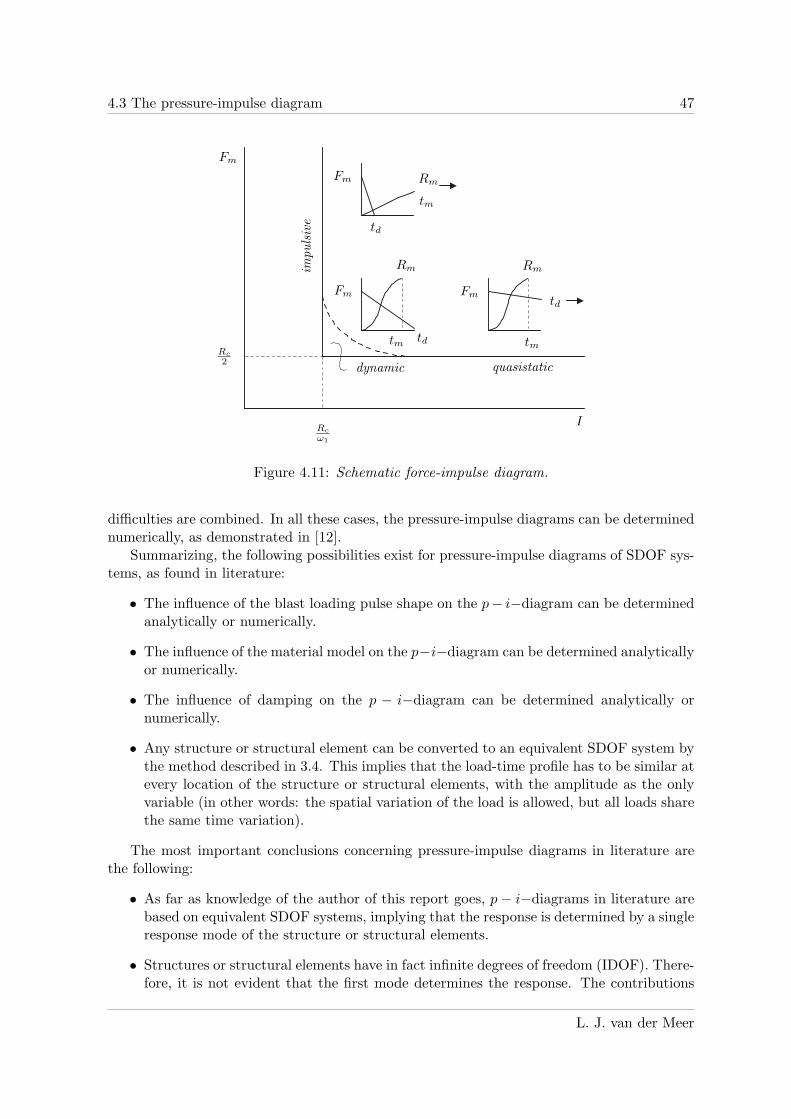
4.3 The pressure-impulse diagram 47
Fm
Fm
Fm
Fm
Rm
Rm
Rm
tm
tm
tmRc
2
Rc
ω1
dynamic quasistatic
impulsiv
e
td
td
td
I
Figure 4.11: Schematic force-impulse diagram.
difficulties are combined. In all these cases, the pressure-impulse diagrams can be determinednumerically, as demonstrated in [12].
Summarizing, the following possibilities exist for pressure-impulse diagrams of SDOF sys-tems, as found in literature:
• The influence of the blast loading pulse shape on the p− i−diagram can be determinedanalytically or numerically.
• The influence of the material model on the p−i−diagram can be determined analyticallyor numerically.
• The influence of damping on the p − i−diagram can be determined analytically ornumerically.
• Any structure or structural element can be converted to an equivalent SDOF system bythe method described in 3.4. This implies that the load-time profile has to be similar atevery location of the structure or structural elements, with the amplitude as the onlyvariable (in other words: the spatial variation of the load is allowed, but all loads sharethe same time variation).
The most important conclusions concerning pressure-impulse diagrams in literature arethe following:
• As far as knowledge of the author of this report goes, p − i−diagrams in literature arebased on equivalent SDOF systems, implying that the response is determined by a singleresponse mode of the structure or structural elements.
• Structures or structural elements have in fact infinite degrees of freedom (IDOF). There-fore, it is not evident that the first mode determines the response. The contributions
L. J. van der Meer
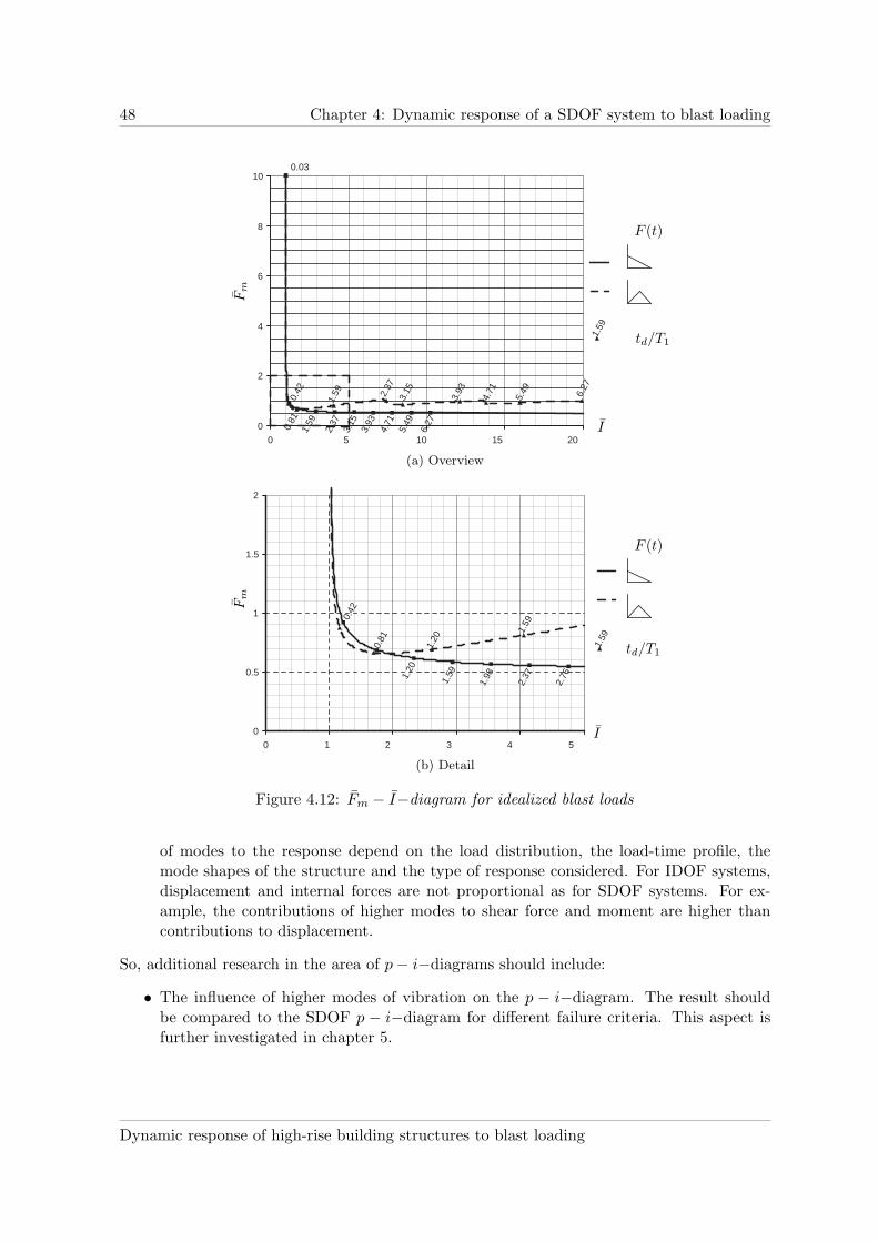
48 Chapter 4: Dynamic response of a SDOF system to blast loading
0
2
4
6
8
10
0 5 10 15 20
0.03
3.93
4.
71
5.49
6.
27
3.15
2.37
1.59
0.81
0.
42
1.59
2.37
3.
15
3.93
4.71
5.49
6.27
1.
59
Fm
I
td/T1
F (t)
(a) Overview
1.59
0
0.5
1
1.5
2
0 1 2 3 4 5
0.42
0.81
1.20
1.59
1.20
1.59
1.98
2.37
2.76
Fm
I
td/T1
F (t)
(b) Detail
Figure 4.12: Fm − I−diagram for idealized blast loads
of modes to the response depend on the load distribution, the load-time profile, themode shapes of the structure and the type of response considered. For IDOF systems,displacement and internal forces are not proportional as for SDOF systems. For ex-ample, the contributions of higher modes to shear force and moment are higher thancontributions to displacement.
So, additional research in the area of p − i−diagrams should include:
• The influence of higher modes of vibration on the p − i−diagram. The result shouldbe compared to the SDOF p − i−diagram for different failure criteria. This aspect isfurther investigated in chapter 5.
Dynamic response of high-rise building structures to blast loading

49
Chapter 5
Dynamic response of a continuousbeam to blast loading
In chapter 4, it was concluded that the influence of higher modes of vibration is not included inthe pressure-impulse-diagram, because the diagram is generally set up for a failure criterium(or a degree of damage) of an equivalent SDOF system. To investigate the influence ofhigher modes of vibration on the response and equivalently, the p − i−diagram, this chapterfocusses on the response of a continuous beam with infinite degrees of freedom, as shown infigure 3.5a but without the rotary spring at the base. It is assumed that the beam has anequally distributed mass, bending stiffness and shear stiffness. As stated before in section3.4, the equivalent beam deduced from a trussed frame is a non-slender beam, which requiresshear deflection to be included. In [9], dynamics of vibration are explained for four typesof beams, of which two include shear deflection. The Timoshenko beam includes both sheardeformation and rotary inertia, which is the effect of rotation of the cross section, in additionto deformation due to bending. Therefore, it is the best available model for non-slenderbeams.
In this chapter, the differential equation of motion of the Timoshenko beam accordingto [9] is described in section 5.1. Subsequently, the natural frequencies and eigenfunctions(mode shapes) of the Timoshenko beam are derived in section 5.2. In section 5.3, orthogonalityand normalization of eigenfunctions, the mode superposition method and modal contributionfactors for base shear and moment are discussed. The mode superposition method uses thesuperposition principle for linear systems to write the response as a sum of modal responses.The modal contribution factors for base shear and moment are derived from similar factorsfor earthquake engineering [7]. In section 5.4, the maximum of the resulting response isapproximated. Finally, in section 5.5, the dynamic load factors of the higher modes areapproximated for impulsive and quasi-static response, to obtain the asymptotes of the p −i−diagram for base shear and moment. The result of this chapter is a p−i−diagram includingthe influence of higher modes of vibration, which can be compared to the SDOF p−i−diagramsof section 4.3.
L. J. van der Meer

50 Chapter 5: Dynamic response of a continuous beam to blast loading
5.1 The differential equation of motion of a transversely vi-brating Timoshenko beam
5.1.1 Dimensionless variables
The equations of motion of a Timoshenko beam are derived in [9]. The dimensionless variablesused in this source will be used here also, but with some adaptations to improve the coherencewith the other parameters used in this report. Axial coordinate x, transverse deflection w,rotation due to bending moment ϕ, time t and natural frequency ωn are made dimensionlessas follows:
x =x
H, w =
w
H, ϕ = ϕ, t = ω1t, ωn =
ωn
ω1(5.1)
The distributed mass m, force P and shear stiffness S are made dimensionless by using B,H, ω1 and the parameter α from (3.22):
m = mH4ω2
1
B, P = P
H3
B, S = α =
s2
γ2= S
k′H2
B(5.2)
The moment µ and shear force v are, as a result, dimensionless:
µ = µH
B, v = v
H2
B(5.3)
The time dependent part of the force F is equal to F in figure 4.4c. In other words, noamplitude is included in the time dependent part of the force.
5.1.2 Equation of motion of a Timoshenko beam
m∂2w(x, t)
∂t2− α
(
∂2w(x, t)
∂x2− ∂ϕ(x, t)
∂x
)
= P (x, t) (5.4)
m
s2
∂2w(x, t)
∂t2− ∂2ϕ(x, t)
∂x2− α
(
∂w(x, t)
∂x− ϕ(x, t)
)
= 0 (5.5)
In these differential equations, the dimensionless parameters from subsection 5.1.1 are usedand s is the slenderness ratio (and not the shear stiffness which is denoted with capital S).
It can be shown that w(x, t) and ϕ(x, t) are of the same form. They can be synchronized intime by assuming that they share the same time solution T (t):
[
w(x, t)ϕ(x, t)
]
= T (t)
[
W (x)Ψ(x)
]
(5.6)
The differential equation can be decoupled into a spatial equation and a time equation. Thetime equation is:
¨T (t) + ω2T (t) = 0 (5.7)
Dynamic response of high-rise building structures to blast loading

5.2 Determination of mode shapes and natural frequencies of a beam 51
The spatial equation is given by
0 =
[
α 0
0 1
] [
W ′′(x)
Ψ′′(x)
]
+
[
0 −α
α 0
] [
W ′(x)
Ψ′(x)
]
+
mω2 0
0mω2
s2− α
[
W (x)
Ψ(x)
]
(5.8)
where the forcing function is set to zero.
5.2 Determination of mode shapes and natural frequencies ofa beam
For the clamped-free Timoshenko beam (i.e. cantilevered), the frequency equation is given in[9] by:
(a2 − b2) sin a sinh b − ab(a4 + a4γ4 + 4γ2a2b2 + b4γ4 + b4)
(b2 + γ2a2)(a2 + γ2b2)cos a cosh b − 2ab = 0 (5.9)
In which a is the wave number, which is 2π times the number of cycles of the eigenfunction(mode shape) in the beam length, b does not have a physical meaning but is a parameter inthe eigenfunction, γ is given in (3.21).
If a < ac, then the frequency equation is exactly as above. When a > ac, the frequencyequation is obtained by replacing b by jb and j2 = −1. The critical wave number ac is givenby:
ac = s
√
1
γ2+ 1 with slenderness ratio s =
√
αγ2 (5.10)
There are two eigenfunctions, one for a < ac and one for a > ac. If a < ac, the vector ofeigenfunctions is given by:
[
W (x)Ψ(x)
]
=
[
C1
D1
]
sin ax +
[
C2
D2
]
cos ax +
[
C3
D3
]
sinh bx +
[
C4
D4
]
cosh bx (5.11)
There are only four unknowns, because Dn and Cn are interrelated by a, b and γ.
D1 = −a2 + γ2b2
(1 + γ2)aC2 D2 =
a2 + γ2b2
(1 + γ2)aC1
D3 =b2 + γ2a2
(1 + γ2)bC4 D4 =
b2 + γ2a2
(1 + γ2)bC3 (5.12)
If a > ac the eigenfunction becomes
[
W (x)Ψ(x)
]
=
[
C1
D1
]
sin ax +
[
C2
D2
]
cos ax +
[
C3
D3
]
sin bx +
[
C4
D4
]
cos bx (5.13)
L. J. van der Meer
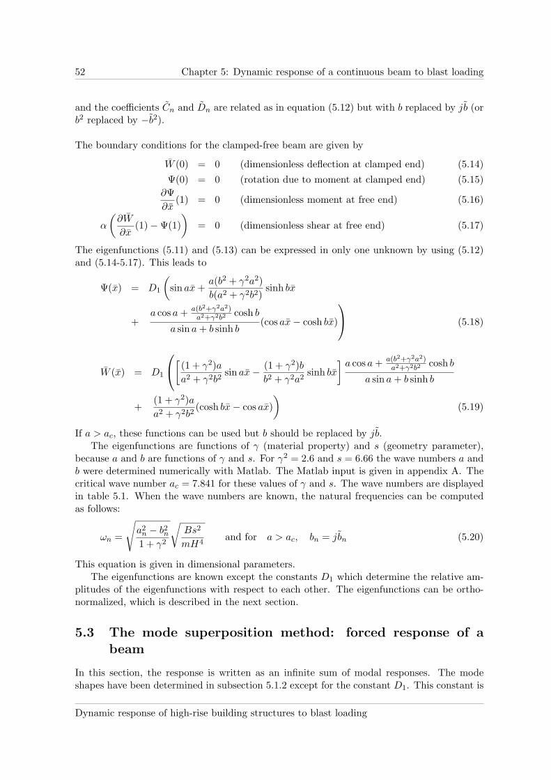
52 Chapter 5: Dynamic response of a continuous beam to blast loading
and the coefficients Cn and Dn are related as in equation (5.12) but with b replaced by jb (orb2 replaced by −b2).
The boundary conditions for the clamped-free beam are given by
W (0) = 0 (dimensionless deflection at clamped end) (5.14)
Ψ(0) = 0 (rotation due to moment at clamped end) (5.15)
∂Ψ
∂x(1) = 0 (dimensionless moment at free end) (5.16)
α
(
∂W
∂x(1) − Ψ(1)
)
= 0 (dimensionless shear at free end) (5.17)
The eigenfunctions (5.11) and (5.13) can be expressed in only one unknown by using (5.12)and (5.14-5.17). This leads to
Ψ(x) = D1
(
sin ax +a(b2 + γ2a2)
b(a2 + γ2b2)sinh bx
+a cos a + a(b2+γ2a2)
a2+γ2b2cosh b
a sin a + b sinh b(cos ax − cosh bx)
(5.18)
W (x) = D1
[
(1 + γ2)a
a2 + γ2b2sin ax − (1 + γ2)b
b2 + γ2a2sinh bx
]
a cos a + a(b2+γ2a2)a2+γ2b2
cosh b
a sin a + b sinh b
+(1 + γ2)a
a2 + γ2b2(cosh bx − cos ax)
)
(5.19)
If a > ac, these functions can be used but b should be replaced by jb.The eigenfunctions are functions of γ (material property) and s (geometry parameter),
because a and b are functions of γ and s. For γ2 = 2.6 and s = 6.66 the wave numbers a andb were determined numerically with Matlab. The Matlab input is given in appendix A. Thecritical wave number ac = 7.841 for these values of γ and s. The wave numbers are displayedin table 5.1. When the wave numbers are known, the natural frequencies can be computedas follows:
ωn =
√
a2n − b2
n
1 + γ2
√
Bs2
mH4and for a > ac, bn = jbn (5.20)
This equation is given in dimensional parameters.The eigenfunctions are known except the constants D1 which determine the relative am-
plitudes of the eigenfunctions with respect to each other. The eigenfunctions can be ortho-normalized, which is described in the next section.
5.3 The mode superposition method: forced response of abeam
In this section, the response is written as an infinite sum of modal responses. The modeshapes have been determined in subsection 5.1.2 except for the constant D1. This constant is
Dynamic response of high-rise building structures to blast loading

5.3 The mode superposition method: forced response of a beam 53
Mode an bn or bn ωn[rad/s] fn[Hz]
1 1.84075 1.62824 2.897305 0.4605472 4.14219 2.52714 11.06107 1.7604243 7.07301 1.63825 23.18962 3.690743
4 8.69907 1.94629 30.04294 4.7814825 10.83199 4.07270 39.00174 6.2073196 11.67560 4.78576 42.52713 6.7684037 14.27275 6.81980 53.31200 8.4848688 15.40061 7.65717 57.96558 9.2255099 17.58377 9.22948 66.92929 10.6521310 19.49123 10.56530 74.72047 11.89213
Table 5.1: Wave number and frequencies for a Timoshenko beam with γ2 = 2.6 and s = 6.66.
different for each mode and has to be determined to obtain the amplitudes of the modes withrespect to the other modes. This can be done by normalization to the mass of the system.For the superposition principle to work properly, it is also necessary that all mode shapes areorthogonal with respect to each other, i.e. non of the mode shapes is allowed to be a linearcombinations of the other mode shapes. In subsection 5.3.1 the ortho-normality condition isgiven, which, if satisfied, guarantees both the orthogonality and normalization to mass of themode shapes.
Once the mode shapes are normalized and orthogonality is satisfied, they can be used ina mode superposition method, which is explained in subsection 5.3.2. When the responseis obtained through this method, the response is an infinite sum of modal responses. It isimpossible and luckily also unnecessary to include infinite modes.
In subsection 5.3.3, modal contribution factors for base shear and moment are defined,which give the contribution of a certain mode in percent. The contribution factors are spe-cialized for base shear and moment, because these are usually critical in a laterally loadedcantilevered beam. Once it is known that a few lower modes contribute for example 95% tothe base shear or moment, then the other modes can be neglected. The total response maybe corrected with a factor to account for the missing 5% or a static correction method can beused if the response of the first mode is quasi-static (paragraph 12.12 of [7]).
5.3.1 Orthogonality and normalization of eigenfunctions
The eigenfunctions or mode shapes can be ortho-normalized using:
1∫
0
(
Wn(x)Wm(x) +1
s2Ψn(x)Ψm(x)
)
dx = δnm (5.21)
where δnm is the Kronecker delta, which is 1 for n = m and 0 otherwise.
This is the orthogonality condition when n 6= m. Equations (5.18) and (5.19) satisfy thiscondition. When n = m the eigenfunctions are normalized according to (5.21), which issolved for the unknown constant D1 in (5.18) and (5.19).
L. J. van der Meer
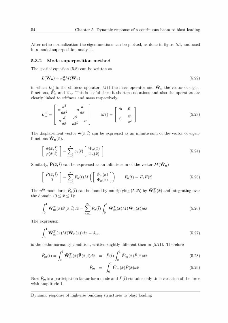
54 Chapter 5: Dynamic response of a continuous beam to blast loading
After ortho-normalization the eigenfunctions can be plotted, as done in figure 5.1, and usedin a modal superposition analysis.
5.3.2 Mode superposition method
The spatial equation (5.8) can be written as
L(Wn) = ω2nM(Wn) (5.22)
in which L() is the stiffness operator, M() the mass operator and Wn the vector of eigen-functions, Wn and Ψn. This is useful since it shortens notations and also the operators areclearly linked to stiffness and mass respectively.
L() =
αd2
dx2−α
d
dx
αd
dx
d2
dx2− α
M() =
m 0
0m
s2
(5.23)
The displacement vector w(x, t) can be expressed as an infinite sum of the vector of eigen-functions Wn(x).
[
w(x, t)ϕ(x, t)
]
=∞
∑
n=1
ηn(t)
[
Wn(x)Ψn(x)
]
(5.24)
Similarly, P(x, t) can be expressed as an infinite sum of the vector M(Wn)
[
P (x, t)0
]
=∞
∑
n=1
Fn(t)M
([
Wn(x)Ψn(x)
])
Fn(t) = FnF (t) (5.25)
The nth mode force Fn(t) can be found by multiplying (5.25) by WTm
(x) and integrating overthe domain (0 ≤ x ≤ 1):
∫ 1
0WT
m(x)P(x, t)dx =
∞∑
n=1
Fn(t)
∫ 1
0WT
m(x)M(Wn(x))dx (5.26)
The expression
∫ 1
0WT
m(x)M(Wn(x))dx = δnm (5.27)
is the ortho-normality condition, written slightly different then in (5.21). Therefore
Fm(t) =
∫ 1
0WT
m(x)P(x, t)dx = F (t)
∫ 1
0Wm(x)P (x)dx (5.28)
Fm =
∫ 1
0Wm(x)P (x)dx (5.29)
Now Fm is a participation factor for a mode and F (t) contains only time variation of the forcewith amplitude 1.
Dynamic response of high-rise building structures to blast loading

5.3 The mode superposition method: forced response of a beam 55
0.2 0.4 0.6 0.8 1
-0.4
-0.2
0.2
0.4
0.6
W1
W2
W3
W4
W5
W6
W7
W8
W9
W10
(a) Deflection
0.2 0.4 0.6 0.8 1
-2
-1
1
2
3
Ψ1
Ψ2
Ψ3
Ψ4
Ψ5
Ψ6
Ψ7
Ψ8
Ψ9
Ψ10
(b) Rotation due to bending moment
Figure 5.1: Eigenfunctions of a Timoshenko beam with γ2 = 2.6 and s = 6.66.
L. J. van der Meer

56 Chapter 5: Dynamic response of a continuous beam to blast loading
The equations of motion (5.4) can be rewritten using (5.24) and (5.25) as
∞∑
n=1
(
¨ηn(t)M(Wn(x)) + ηn(t)L(Wn(x)))
=
∞∑
n=1
FnM(Wn(x))F (t) (5.30)
Using (5.22) this can be simplified to
∞∑
n=1
(
¨ηn(t) + ω2nηn(t)
)
M(Wn(x)) =∞
∑
n=1
FnM(Wn(x))F (t) (5.31)
which after multiplying by WTm
(x), integrating over the domain (0 ≤ x ≤ 1) and usingortho-normality becomes
¨ηm(t) + ω2mηm(t) = Fm(t) for every m = 1, 2, ..∞ (5.32)
Equation (5.32) is equivalent to the equation of motion of a SDOF system and the samesolutions for the dynamic load factor can be used within every mode. The complete solutionis the infinite sum of these modes.
[
w(x, t)ϕ(x, t)
]
=∞
∑
n=1
ηn(t)
[
Wn(x)Ψn(x)
]
=∞
∑
n=1
Fn
ω2n
Dn(t)
[
Wn(x)Ψn(x)
]
(5.33)
where Dn(t) is the dynamic load factor (DLF) obtained by applying F (t) to a SDOF system.
Dimensionless moment µ and shear force v can be derived from (5.33) directly.
µ(x, t) =∂ϕ(x, t)
∂x=
∞∑
n=1
Fn
ω2n
Dn(t)dΨn(x)
dx(5.34)
v(x, t) = α
(
∂w(x, t)
∂x− ϕ(x, t)
)
=∞
∑
n=1
Fn
ω2n
Dn(t)α
(
dWn(x)
dx− Ψn(x, t)
)
(5.35)
For the dimensional quantities w(x, t), µ(x, t) and v(x, t) the dimensionless quantities shouldbe multiplied by H, B/H and B/H2 respectively and the dynamic load factor D(t) for theforce F (t) should be used with t instead of t as the variable.
5.3.3 Modal contribution factors
In [7] in paragraph 16.6, an alternative method to calculate base shear and moment is given.This method can also be used to derive modal contribution factors for base shear and mo-ment. Modal contribution factors give the ratio of the quantity in the nth mode to the sum ofall modes, without having to calculate all modes first. The method in the book is specializedfor base acceleration, but the same principle can be used for an arbitrary applied force as well.
Equation (5.22) is repeated here:
L(Wn(x)) = ω2nM(Wn(x)) (5.36)
Dynamic response of high-rise building structures to blast loading
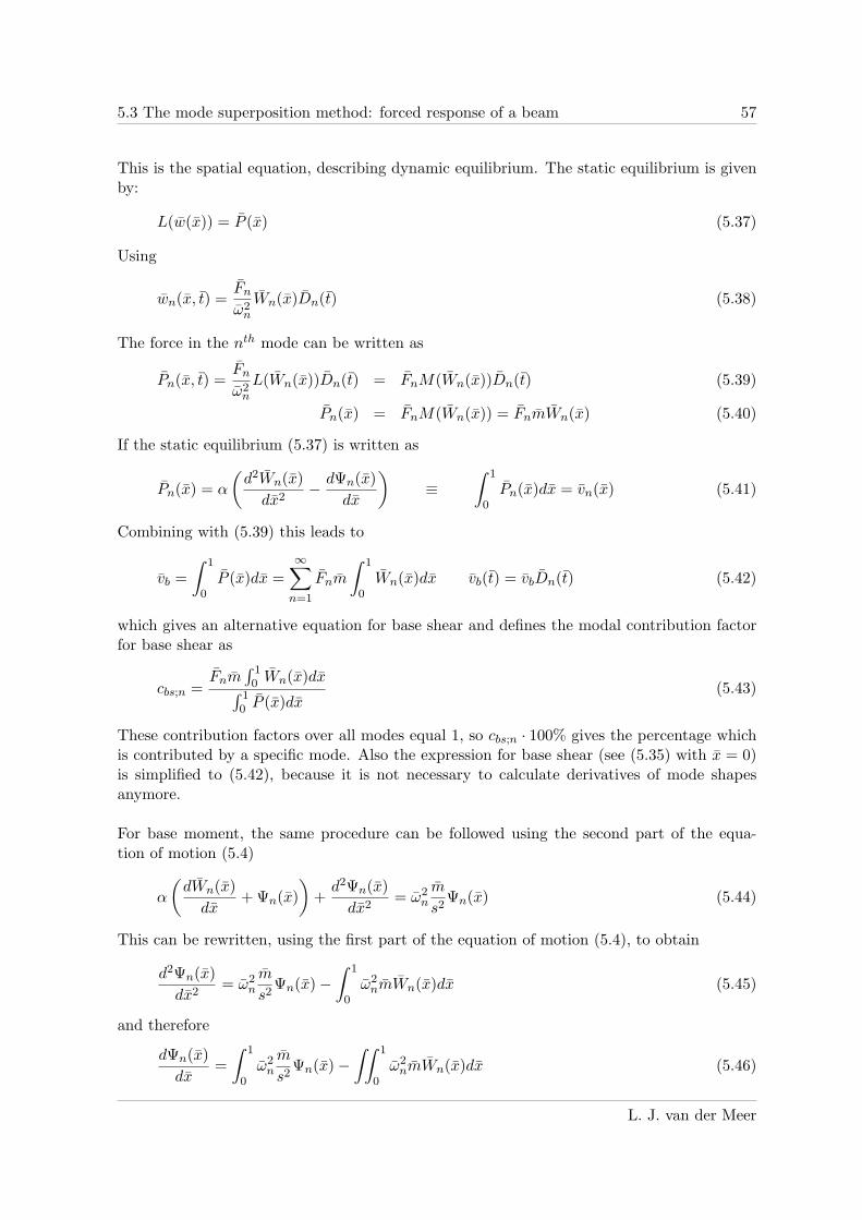
5.3 The mode superposition method: forced response of a beam 57
This is the spatial equation, describing dynamic equilibrium. The static equilibrium is givenby:
L(w(x)) = P (x) (5.37)
Using
wn(x, t) =Fn
ω2n
Wn(x)Dn(t) (5.38)
The force in the nth mode can be written as
Pn(x, t) =Fn
ω2n
L(Wn(x))Dn(t) = FnM(Wn(x))Dn(t) (5.39)
Pn(x) = FnM(Wn(x)) = FnmWn(x) (5.40)
If the static equilibrium (5.37) is written as
Pn(x) = α
(
d2Wn(x)
dx2− dΨn(x)
dx
)
≡∫ 1
0Pn(x)dx = vn(x) (5.41)
Combining with (5.39) this leads to
vb =
∫ 1
0P (x)dx =
∞∑
n=1
Fnm
∫ 1
0Wn(x)dx vb(t) = vbDn(t) (5.42)
which gives an alternative equation for base shear and defines the modal contribution factorfor base shear as
cbs;n =Fnm
∫ 10 Wn(x)dx
∫ 10 P (x)dx
(5.43)
These contribution factors over all modes equal 1, so cbs;n · 100% gives the percentage whichis contributed by a specific mode. Also the expression for base shear (see (5.35) with x = 0)is simplified to (5.42), because it is not necessary to calculate derivatives of mode shapesanymore.
For base moment, the same procedure can be followed using the second part of the equa-tion of motion (5.4)
α
(
dWn(x)
dx+ Ψn(x)
)
+d2Ψn(x)
dx2= ω2
n
m
s2Ψn(x) (5.44)
This can be rewritten, using the first part of the equation of motion (5.4), to obtain
d2Ψn(x)
dx2= ω2
n
m
s2Ψn(x) −
∫ 1
0ω2
nmWn(x)dx (5.45)
and therefore
dΨn(x)
dx=
∫ 1
0ω2
n
m
s2Ψn(x) −
∫∫ 1
0ω2
nmWn(x)dx (5.46)
L. J. van der Meer

58 Chapter 5: Dynamic response of a continuous beam to blast loading
Remembering that (5.34)
µn(x, t) =Fn
ω2n
Dn(t)dΨn(x)
dx(5.47)
and substituting (5.46), the alternative expression for base moment is obtained:
µb;n = Fnm
(
1
s2
∫ 1
0Ψn(x)dx +
∫ 1
0xWn(x)dx
)
µb;n(t) = µb;nDn(t) (5.48)
Therefore the contribution factor for base moment is defined as
cbm;n =Fnm
(
1s2
∫ 10 Ψn(x)dx +
∫ 10 xWn(x)dx
)
∫ 10 xP (x)dx
(5.49)
In table 5.2 the modal contribution factors are compared for base shear and moment, forthree different load distributions (similar to the load distributions used in section 3.4):
• Uniform distribution: P (x) = Pm
• Linear distribution: P (x) = 2Pm(1 − x)
• Quadratic distribution: P (x) = 3Pm(x − 1)2
In these expressions the amplitudes are chosen so that∫ 10 P (x)dx = Pm. This is not necessary
for evaluation of the contribution factors but it gives the load distributions the same area whenthey are plotted, see figure 5.2. In table 5.2, the bold contribution factors represent a totalcontribution of 95% for base moment and 90% for base shear. It can be seen that higher modescontribute more to base shear than to base moment. Also, when the load distribution is notuniform but more concentrated at the base, as is likely for a blast load from a short-rangeexplosion, the higher modes have more influence.
Load distribution→ Uniform Linear QuadraticMode↓ Shear[%] Moment[%] Shear[%] Moment[%] Shear[%] Moment[%]
1 61.48 92.49 35.93 81.08 24.20 72.80
2 23.35 6.78 34.96 15.24 34.40 19.99
3 5.93 0.98 12.36 3.07 16.63 5.51
4 1.68 -0.40 0.92 -0.33 1.89 -0.905 1.43 0.41 3.77 1.64 5.33 3.096 0.78 -0.33 1.49 -0.96 1.52 -1.307 0.97 0.18 1.80 0.51 3.06 1.168 0.25 -0.14 0.46 -0.38 0.62 -0.689 0.60 0.12 1.31 0.39 1.85 0.7310 0.25 -0.13 0.46 -0.36 0.69 -0.72
Sum 96.72 99.96 93.46 99.90 90.19 99.68Sum 90.76 99.27 90.31 96.32 90.19 98.30
Table 5.2: Modal contribution factors in % for base shear and moment.
Dynamic response of high-rise building structures to blast loading

5.4 Approximation of response including higher modes 59
0.2 0.4 0.6 0.8 1
0.5
1
1.5
2
2.5
3
P (x)
x
uniform
quadratic
linear
Figure 5.2: Three different load distributions.
5.4 Approximation of response including higher modes
From subsection 5.3.3, the contributions of each mode to the total dynamic response are knownand the transient response can be plotted. However, the construction of a p− i−diagram re-quires the maximum response to be determined. Unfortunately, the response is a sum ofharmonic functions, of which the global maximum is difficult to determine. For earthquakeengineering, several modal combination rules have been established [7]. These modal com-bination rules use the modal maxima to estimate the total maximum of response and aredescribed in subsection 5.4.1.
Another problem arises here, because the n−th modal maximum, determined by thedynamic load factor for mode n, is influenced by the response of the mode with the highestcontribution, usually the first mode. For example, if the maximum response of the firstmode occurs just after td, then all higher modes have their first maximum before td, whichdetermines the dynamic load factor. However, if the first mode has the highest contribution,then the overall maximum response is likely to occur near the maximum of the first mode.The maxima of the higher modes in this region are lower than their first maxima. So theregime of the response of the first mode (impulsive, dynamic or quasi-static) influences thedynamic load factors of the higher modes. This is elaborated in subsection 5.4.2.
Finally, the modal maxima and the modal combination rules are used to estimate themaximum response in subsection 5.4.3.
5.4.1 Modal combination rules
Modal combination rules are described in paragraph 13.7.2 of [7] of which only two are dis-cussed here. They will be used to approximate maximum base moment and base shearincluding influence of the higher modes. The problem with determining the maximum dy-namic response of a continuous or MDOF system, is that the total response is a combinationof dynamic load factors Dn(t) with different contribution factors.
The absolute sum (ABSSUM) modal combination rule is defined as the absolute sum of themaximum response of all modes. Since the Dn(t) vary sinusoidally with different frequencies,the actual maximum is always lower than the maximum from the absolute sum rule. If the
L. J. van der Meer

60 Chapter 5: Dynamic response of a continuous beam to blast loading
maximum of a response quantity is denoted as rm;abssum, the rule can be written as:
rm;abssum 'N
∑
n=1
|rm;n| (5.50)
Where n = 1..N are the modes that have a significant contribution to the response quantityaccording to the modal contribution factors. This rule is (very) conservative and thereforenot popular in structural design applications.
The square-root-of-sum-of-squares rule (SRSS) gives a less conservative approximation ofthe maximum of a response quantity. If the maximum of a response quantity is denoted asrm;srss, the rule can be written as
rm;srss '
√
√
√
√
N∑
n=1
r2m;n (5.51)
Where n = 1..N are the modes that have a significant contribution to the response quantityaccording to the modal contribution factors. The SRSS rule is based on random vibrationtheory and specialized for earthquake engineering, hence it is less accurate for blast loading.
5.4.2 Dynamic load factor including higher modes
The dynamic load factor for higher modes of vibration is approximated for the differentregimes in the p-i diagram, assuming an idealized detonation as in figure 4.3a. For an idealizeddeflagration the method is similar. The method is divided in a conservative approach and aless conservative approach.
Time dependent vs maximum dynamic load factor
The time dependent dynamic load factor is denoted as Dn(t) and defined as the time dependentdynamic response of mode n divided by the static response if the maximum dynamic load wereapplied statically. The maximum dynamic load factor Dm;n is defined as the first maximumof the dynamic respons of mode n divided by the static response if the maximum dynamicload were applied statically.
Conservative approach
The conservative approach is to assume that the dynamic load factor of all modes is deter-mined by either the quasi-static or the impulsive asymptote. The dynamic regime in betweenthe asymptotes is ignored. The maximum dynamic load factor is Dm;n = 2 (idealized deto-nation) on the quasi-static asymptote and Dm;n = ωntd/2. This is shown in figure 5.3. Forhigher modes, td/Tn becomes larger, as is indicated in this figure.
The maximum response in the quasi-static regime equals the response to a step force,which is equal to the value 2, independent of the natural frequency. If the load is a step forcefor the lowest natural frequency, it will also be a step force for the higher natural frequencies.Therefore, the maximum dynamic load factor Dm;n is equal to 2 for all modes. In figure 5.4the time-dependent response of 3 modes is shown. The maximum of each mode is equal tothe modal contribution factor cb;n multiplied by Dm;n. The modal contribution factors forbase shear, uniform distributed loading, from table 5.2 are used, normalized to 100%.
Dynamic response of high-rise building structures to blast loading

5.4 Approximation of response including higher modes 61
0
1
2
0 1 2 3 4 5 6 0.64
td/Tn
F (t)
impulsive quasi-static
Dm
;n
approximation
exact value
higher modes
dynamic
Fm
Fm
Fm
Rm
Rm
Rm
tm
tm
tmtd
td
td
Figure 5.3: Dynamic load factor and asymptotes for an idealized detonation.
0 0.2 0.4 0.6 0.8 1 1.2 1.4 1.6 1.8 2
-1
-0.5
0
0.5
1
1.5
2
c b;n·D
n(t
)
t [s]
1st mode, quasi-static
2nd mode, quasi-static
3rd mode, quasi-static
sum of 3 modes
step force
modal maximum
total maximum
Figure 5.4: Quasi-static base shear response of 3 modes to step force (uniform distribution).
L. J. van der Meer

62 Chapter 5: Dynamic response of a continuous beam to blast loading
The maximum response in the impulsive regime on the other hand, is determined by thenatural frequency, because the dynamic load factor is determined by the impulsive asymptote,Dm;n = ωntd/2 = πtd/Tn. This is only the case when all modes with a significant contributionare in the impulsive regime. This means that all significant modes should have a ratio oftd/Tn < 0.64, see figure 5.3. The time dependent response of 3 modes is shown in figure 5.5for an idealized detonation with td = 0.1s. The natural frequencies are taken from table 5.1.The td/Tn ratios are 0.046, 0.176 and 0.369 respectively, which are all in the impulsive regime(although the third mode is only just within the impulsive regime).
-0.3
-0.2
-0.1
0
0.1
0.2
0.3
0 0.2 0.4 0.6 0.8 1 1.2 1.4 1.6 1.8 2
c b;n·D
n(t
)
t [s]
td
1st mode, impulsive
2nd mode, impulsive
3rd mode, impulsive
sum of 3 modes
impulse
modal maximum
total maximum
Figure 5.5: Impulsive base shear response of 3 modes to idealized detonation (uniform distri-bution).
Less conservative approach
The less conservative approach described here, applies only when the first mode has thelargest contribution to the response. It uses the td/Tn−values of the higher modes to predictthe maximum dynamic load factors Dm;n of the higher modes including the dynamic regime.These maximum dynamic load factors depend on the maximum dynamic load factor of thefirst mode Dm;1. There are two possibilities:
• The maximum of the first mode occurs during forced vibration (tm;1 < td). This isresponse in the dynamic regime close to the quasi-static regime.
• The maximum of the first mode occurs during free vibration (tm;1 > td). This is responsein the dynamic regime close to the impulsive regime.
Response in the dynamic regime, close to the quasi-static regime, is shown for 3 modes infigure 5.6b for td = 2 s. The location of the modes is shown in the Dm − td/Tn−plot of figure5.6a. If it is assumed that the first mode has the highest contribution factor, as is the casein figure 5.6b, its maximum response governs the total response. The higher modes reachtheir first maximum earlier due to their shorter periods of vibration, but these maxima tonot contribute to the maximum total response. Therefore, they are indicated in figure 5.6band figure 5.6a as ’false’ maxima.
Dynamic response of high-rise building structures to blast loading

5.4 Approximation of response including higher modes 63
0
1
2
0 1 2 3 4 5 6 0.64
modal maximum
’false’ maximum
td/Tn
F (t)
Dm
;n
approximation
exact value
higher modes
conservativemore conservative
1st mode 2nd mode 3rd mode
(a) Maximum dynamic load factor Dn;m
0 0.2 0.4 0.6 0.8 1 1.2 1.4 1.6 1.8 2
-1
-0.5
0
0.5
1
1.5
2
c b;n·D
n(t
)
t [s]
1st mode, dynamic
2nd mode, dynamic
3rd mode, dynamic
sum of 3 modes
F (t)
modal maximum
total maximum
’false’ maximum
td
(b) Modal responses cb;nDn(t)
0 0.2 0.4 0.6 0.8 1 1.2 1.4 1.6 1.8 2
-1
-0.5
0
0.5
1
1.5
2
t [s]
F (t)
modal maximum
’false’ maximum
1st mode
2nd mode
3rd mode
Dn(t
)
F (t) + 1
(c) Time dependent dynamic load factor Dn(t)
Figure 5.6: Quasi-static/dynamic base shear response of 3 modes to idealized detonation (uni-form distribution).
L. J. van der Meer

64 Chapter 5: Dynamic response of a continuous beam to blast loading
In figure 5.6c the dynamic load factors Dn(t) for 3 modes are shown without their con-tribution factors. The time dependent dynamic load factor Dn(t) is approximately equal toF (t) + 1. Since the modal maxima of the first and higher modes occur at approximately thesame time, Dm;n ≈ Dm;1. It is conservative to use the ’false’ maxima, which are simply theDm;n for the td/Tn−values of the modes involved (indicated in the figure with a triangle).
Response in the dynamic regime, close to the impulsive regime, is characterized by one ormore modes in the impulsive regime and a number of higher modes in the dynamic regime.The MDOF or continuous impulsive response is a limit case, because there are always highermodes outside the impulsive regime. These modes have often small contribution factors,but high dynamic load factors, if they are determined by the impulsive asymptote. On theimpulsive asymptote Dm;n = ωntd/2, hence the dynamic load factor is determined by ωn
which increases with mode number. If all higher modes are approximated by this dynamicload factor, almost all higher modes would have a significant contribution. However, modeswith high frequencies fall outside the impulsive regime. In figure 5.7b the response in thedynamic regime near the impulsive regime is shown for 3 modes, td = 0.5 s. In this case,the first mode response is impulsive, while the second and third mode attain their maximaduring the presence of the force. However, these maxima during forced vibration are ’false’maxima, since they do not contribute to the total maximum. Instead the maxima of freevibration should be determined. This can be shown by calculating the dynamic load factorfor free vibration (substitute tm for tm > td (4.16) in D(t) (4.11)), which is compared toforced vibration in figure 5.7a. For an idealized detonation, Dn ≈ 1.25 is a conservativeapproximation for higher modes outside the impulsive regime. For more accurate dynamicload factors, td/Tn values should be calculated and accompanying Dm;n should be determinedwith figure 5.7a.
Summary
The conservative and less conservative approach for determination of maximum dynamic loadfactors of the higher modes are summarized in table 5.3 for an idealized detonation. For anidealized deflagration, figure 5.8 should be used.
Approach → Conservative Less conservative
Time of maximum response offirst mode tm;1 ↓ Asymptotes (limits) Including dynamic regime
tm;1 > td All modes impulsive (td → 0)First mode(s) impulsive, highermodes dynamic
(maximum during free vibration) Dm;n ≈ ωntd2
Dm;n ≈ min
(
ωntd2
, 1.25
)
tm;1 < td Response to step force (td → ∞)All modes dynamic
(maximum during forced vibra-tion)
Dm;n ≈ 2 Dm;n ≈ Dm;1
Table 5.3: Summary: maximum dynamic load factors for higher modes (idealized detonation).
Dynamic response of high-rise building structures to blast loading

5.4 Approximation of response including higher modes 65
0
1
2
0 1 2 3 4 5 6 0.40
1.25
modal maximum
’false’ maximum
td/Tn
F (t)
forced
free
Dm
;n
approximation higher modes
impulsive first maximum
maxima after force1st
2nd
3rd
(a) Maximum dynamic load factor
0 0.2 0.4 0.6 0.8 1 1.2 1.4 1.6 1.8 2
-1
-0.8
-0.6
-0.4
-0.2
0
0.2
0.4
0.6
0.8
1
c b;n·D
n(t
)
t [s]
1st mode, impulsive
2nd mode, dynamic
3rd mode, dynamic
sum of 3 modes
F (t)
modal maximum
total maximum
’false’ maximum
(b) Time dependent dynamic load factor
Figure 5.7: Impulsive/dynamic base shear response of 3 modes to idealized detonation.
L. J. van der Meer

66 Chapter 5: Dynamic response of a continuous beam to blast loading
Idealized deflagration
For an idealized deflagration the maximum dynamic load factors for the first and higher modescan be determined with figure 5.8. There is no obvious approximation for higher modes if thefirst mode is impulsive, so the values of Dm;n should be read from the free vibration part ofthe figure for the values of td/Tn involved.
0
1
2
0 1 2 3 4 5 6
td/Tn
F (t)
forced
freeDm
;n
impulsive
maxima after force
first maximum after maximum force
Figure 5.8: Dynamic load factor for forced and free vibration for idealized deflagration.
5.4.3 Estimates of maximum response
Using the approximations for the dynamic load factors of higher modes, the SRSS rule formodal combination and the expressions for base shear (5.42) and base moment (5.48), theapproximated base shear and moment can be written as:
vb;m = m
√
√
√
√
N∑
n=1
(
FnDn;m
∫ 1
0Wn(x)dx
)2
(5.52)
µb;m = m
√
√
√
√
N∑
n=1
(
FnDn;m1
s2
[∫ 1
0Ψn(x)dx +
∫ 1
0xWn(x)dx
])2
(5.53)
in which Dn;m are the approximations for the dynamic load factors as described in subsection5.4.2.
5.5 Pressure-impulse diagram including higher modes
Only the quasi-static and impulsive criteria from subsection 5.4.2 are needed for the asymp-totes of the p − i−diagram. Denoting the pressure and impulse for the diagram as Pm andJ = Pmtd/2, (5.52) and (5.53) can be rewritten for the impulsive and quasi-static regimes,using Dn;m for the quasi-static or impulsive regime. If we denote:
P (x) =P (x)
Pm→ P (x) = P (x)Pm = P (x)
PmH3
B(5.54)
Dynamic response of high-rise building structures to blast loading

5.5 Pressure-impulse diagram including higher modes 67
then
vb;m = vb;mB
H2= PmH
1∫
0
P (x)dx
√
√
√
√
∞∑
n=1
(Dn;mcbs;n)2 (5.55)
The quasi-static asymptote is obtained by substituting Dn;m = 2 and solving vb;m = vc forPm;vc:
Pm;vc =vc
2H1∫
0
P (x)dx
√
∞∑
n=1c2bs;n
(5.56)
The similar procedure can be followed for base moment, which results in:
µb;m = µb;mB
H= PmH2
1∫
0
xP (x)dx
√
√
√
√
∞∑
n=1
(Dn;mcbm;n)2 = µc (5.57)
and
Pm;mc =µc
2H21∫
0
xP (x)dx
√
∞∑
n=1c2bm;n
(5.58)
For the impulsive asymptotes Dn;m = ωntd/2 should be substituted. Notice that
Dn;mPm =ωntdPm
2= ωnJ with J =
I
H(5.59)
vb;m = vb;mB
H2= HJ
1∫
0
P (x)dx
√
√
√
√
∞∑
n=1
(ωncbs;n)2 = vc (5.60)
Jvc =vc
H1∫
0
P (x)dx
√
∞∑
n=1(ωncbs;n)2
(5.61)
µb;m = H2J
1∫
0
xP (x)dx
√
√
√
√
∞∑
n=1
(ωncbm;n)2 = µc (5.62)
Jmc =µc
H21∫
0
xP (x)dx
√
∞∑
n=1(ωncbm;n)2
(5.63)
A very important conclusion regarding the impulsive response, is that the influence of thehigher modes is not only increased because of the higher contribution factors but also becauseof the natural frequency, which increases with the mode number. Therefore, for impulsiveresponse, the modal contribution factors should be adjusted to account for the influence ofthe natural frequency. The results of these adjustments are shown in table 5.4 and comparedto the quasi-static contribution factors. Both contribution factors are normalized so that thesum over 10 modes is 100%.
L. J. van der Meer

68 Chapter 5: Dynamic response of a continuous beam to blast loading
Shear[%] Moment[%]Mode Quasi-static Impulsive Quasi-static Impulsive
1 63.56 21.23 92.53 75.372 24.14 30.81 6.78 21.123 6.13 16.41 0.98 6.404 1.74 6.02 -0.40 -3.385 1.48 6.65 0.41 4.506 0.81 3.96 -0.33 -3.957 1.00 6.17 0.18 2.708 0.26 1.73 -0.14 -2.299 0.62 4.79 0.12 2.2610 0.26 2.23 -0.13 -2.74
(a) Uniform load distribution
Shear[%] Moment[%]Mode Quasi-static Impulsive Quasi-static Impulsive
1 38.44 8.25 81.16 47.692 37.41 30.69 15.26 34.263 13.22 22.75 3.07 14.474 0.98 2.19 -0.33 -2.025 4.03 11.67 1.64 13.006 1.59 5.03 -0.96 -8.307 1.93 7.62 0.51 5.538 0.49 2.12 -0.38 -4.489 1.40 6.96 0.39 5.3110 0.49 2.73 -0.36 -5.47
(b) Linear load distribution
Shear[%] Moment[%]Mode Quasi-static Impulsive Quasi-static Impulsive
1 26.83 4.55 73.03 34.242 38.14 24.71 20.05 35.943 18.44 25.04 5.53 20.774 2.10 3.69 -0.90 -4.395 5.91 13.50 3.10 19.596 1.69 4.20 -1.30 -8.997 3.39 10.59 1.16 10.058 0.69 2.33 -0.68 -6.419 2.05 8.04 0.73 7.9410 0.77 3.35 -0.72 -8.74
(c) Quadratic load distribution
Table 5.4: Modal contribution factors for 10 modes, quasi-static vs impulsive.
Dynamic response of high-rise building structures to blast loading

69
Chapter 6
Results for example buildingstructure
In this final chapter, the response of the example building structure from chapter 3 to aBLEVE blast according to Baker’s method [23] as well as Van den Berg [21] is determined.The chapter has the same structure as the report itself. Firstly, in section 6.1, the blastload pressure and impulse distribution on the building are determined according to chapter 2.Secondly, the building structure is modeled as an equivalent beam and an equivalent SDOFsystem in section 6.2 as described in chapter 3. Subsequently, the SDOF response as describedin chapter 4 is elaborated in section 6.3. The response of the continuous equivalent beamis given in section 6.4 by the methods of chapter 5. Finally, the results of the SDOF andcontinuous response are compared in section 6.5.
6.1 BLEVE blast loading on example building
Consider a BLEVE blast at the surface from a cylindrical vessel of 108 m3 containing propane,70 volume % liquid, flashing from 329 K at ranges of 20, 35 and 50m from the center ofthe base of the building. The method described in section 2.3, called Baker’s method, isused to determine the free field overpressure and impulse for a surface burst. Alternatively,overpressure and positive phase duration are estimated by using the BLEVE blast charts forpropane in half space, presented in [21], which shall be referred to as Van den Berg’s method.
To determine positive phase duration for Baker’s method or the impulse for Van denBerg’s method, a blast pressure-time profile is needed. From literature, such as [21] and [6],it is concluded that a BLEVE blast pressure-time profile corresponds more to an idealizeddetonation than to an idealized deflagration. In other words, the blast wave from a BLEVE issimilar to a shock wave and not to a pressure wave which is caused by ordinary gas explosions.
In Baker’s method the overpressure and impulse are adjusted for the cylindrical shape ofthe vessel (instead of hemispherical) and the elevation of the vessel above the surface. Thesemodifications increase the overpressure and impulse. Therefore, the same modifications arealso applied to Van den Berg’s overpressure and impulse. The two methods are comparedin table 6.1. It is known that Baker’s method is less accurate for close range, which can beobserved. Furthermore, assuming an idealized blast (detonation pressure-time profile) leadsto short positive phase durations for Baker’s method and high impulses for Van den Berg’smethod.
L. J. van der Meer

70 Chapter 6: Results for example building structure
Baker’s method Van den Berg’s methodr[m] p[kPa] i[kPa·ms] td[ms] p[kPa] i[kPa·ms] td[ms]20 648 1723 5.3 320 6720 4235 130 495 7.6 130 3120 4850 59 280 9.5 54 1350 50
Table 6.1: Free field overpressure, impulse and positive phase duration for a BLEVE usingtwo methods.
6.1.1 Blast distribution
Blast parameters versus scaled distance are available in figures of [3], which are figures 2.6and 2.9 in this report. The overpressure can be used to derive other parameters such as thereflection coefficient and the wavefront velocity versus scaled distance. The wavefront velocityu is needed to determine the time of diffraction of the blast wave around the building to findout whether it is a drag target, a diffraction target or a sequentially loaded target. Theoverpressure and positive phase duration should be determined with Van den Berg’s method[21] and the impulse should be determined by assuming a pressure-time profile. Impulse andpositive phase duration from the figures in [3] should not be used.
Firstly, figure 2.9 is used to determine the amount of TNT (kg) that would produce thesame overpressure. The results are shown in table 6.2.
Baker’s method Van den Berg’s methodr[m] [kg TNT] [kg TNT]20 2950 117035 1875 187550 1650 1400
Table 6.2: Charge mass of a BLEVE at different ranges.
Secondly, the equivalent amount of TNT can be used to estimate the wavefront velocityu and approximate the time of diffraction around the front of the building by:
tdif ;f ≈ 3 min(W/2, H)
u(6.1)
This approximation is found in literature, for example [22] and [19]. Values of the time ofdiffraction around the front between 87-182ms were found. This is longer than the positivephase duration td which is between 5.3-50ms at the ranges considered. Therefore it is con-cluded that the building is a sequentially loaded target for the BLEVE and ranges considered.The pressure-time profile can be approximated by figure 2.8c.
Thirdly, the overpressure in kg TNT can be used to determine pr from figure 2.9 directly.However, then the effect of the angle of incidence on the reflected overpressure is not takeninto account. Therefore, the values of p from table 6.1 are used to determine the reflectioncoefficient Cr. Then Cr is multiplied by p to obtain pr. This is done for every location onthe front of the building for the appropriate values of r and αi, see figure 6.1. This is donenumerically with the Excel program and the average overpressure on the facade is calculated,multiplied by the facade area and divided by the number of stability elements to obtain Fm,the average force on one stability element. The average impulse I, is obtained by using the
Dynamic response of high-rise building structures to blast loading

6.2 Modeling of example building structure 71
td value at the given range and the load-time profile. These are shown in table 6.3. Someimportant assumptions have to be made to obtain these values:
• The pressure-time profile is that of an idealized detonation as shown in figure 2.8c.
• The time of blast arrival ta and the positive phase duration td are set equal at everylocation on the building facade. This is probably conservative since more load is assumedat one time instant than is actually present. However, the dynamic response to asequential load which arrives first at the base and later at the top of the building (seefigure 2.10b) should be evaluated numerically to confirm this assumption.
W
H
L
αi
r
Figure 6.1: Range r and angle of incidence αi for a blast on a facade
Baker’s method Van den Berg’s methodr[m] Fm[MN] I[MN·ms] td[ms] Fm[MN] I[MN·ms] td[ms]20 198 525 5.3 89 1869 4235 76 289 7.6 76 1824 4850 47 223 9.5 42 1050 50
Table 6.3: Average force and impulse from a BLEVE on a facade, transferred to a singlestability element.
6.2 Modeling of example building structure
In section 6.1 the force and impulse on the example building were determined. In this sectiontwo steps of modeling are demonstrated, following chapter 3. The first step, from buildingstructure to trussed frame, is skipped, because the force and impulse are already divided overthe stability elements. The mass is simply calculated for one stability element. The columnsbehind the facade carry some mass as well, but this mass does not affect the mass-stiffnessratio of the stability element. Hence the mass on the stability element is only the mass thatis actually carried by the element (see figure 3.2).
L. J. van der Meer

72 Chapter 6: Results for example building structure
6.2.1 From trussed frame to equivalent beam
The properties of the trussed frame are shown in table 6.4. The bending stiffness B is
H[m] 64.8a[m] 7.2h[m] 3.6d[m] 5.09
E[N/m2] 2.1 · 1011
Ac[m2] 0.09481
Ad[m2] 0.01414
m[kg/m] 31778
Table 6.4: Trussed frame properties.
calculated according to equation (3.2):
B =a2
2EAc =
(7.2)2
2· 2.1 · 1011 · 0.09481 = 5.16 · 1011Nm2 (6.2)
The shear stiffness S is calculated according to equation (3.3):
S =a2h
2d3EAd =
(7.2)2 · 3.6
2 · (5.09)3· 2.1 · 1011 · 0.01414 = 2.10 · 109N (6.3)
The load P (x) on the beam is a function of Pm = Fm/H. One of the three load distributionsfrom figure 3.6 can be chosen for further calculations. The actual load distribution as shownin figure 2.10a is to complex to obtain analytical results. The linear and quadratic loaddistributions model the fact that the blast load is more concentrated at the base (at time ofblast arrival). The linear distribution is chosen in the example.
The equivalent beam is modeled without the rotary spring at the base, because the modeshapes and natural frequencies of a Timoshenko beam with a rotary spring at the base areunknown. The equivalent SDOF response can be obtained using the load-mass factors fromsubsection 3.4.4, but they can not be compared to the equivalent beam response.
6.2.2 From equivalent beam to equivalent SDOF system
First the mass M , stiffness K and force F for the non-equivalent SDOF system are calculatedusing (3.8). The load is assumed to be linear distributed as (3.12):
F =
H∫
0
P (x)dx = PmH = Fm (see table 6.3)
M = mH = 31778 · 64.8 = 2.06 · 106kg
K =F
y(H)=
PmH
PmH4
15B+
PmH2
3S
=1
H3
15B+
H
3S
= 2.20 · 107N/m (6.4)
Now the load-mass factor KLM can be obtained from table 3.4 with the parameter α equalto:
α =s2
γ2=
SH2
B2= 17.09 (6.5)
Dynamic response of high-rise building structures to blast loading

6.3 Single degree of freedom response 73
So:
KLM =5(4455 + 1078α + 75α2)
66(5 + α)(63 + 5α)= 1.035 (6.6)
The natural frequency is equal to:
ω1 =K
KLMM=
√
2.20 · 107
1.035 · 2.06 · 106= 3.21rad/s f1 =
ω1
2π= 0.51Hz (6.7)
It was already concluded in section 3.4 that the natural frequency is approximated less accu-rately by the linear and quadratic load distribution compared to the uniform distribution. Inthe case of uniform distributed loading, f1 = 0.48Hz.
6.3 Single degree of freedom response
First an idea of the response regime can be acquired by calculating the td/T1 ratio. This isdone for the highest positive phase duration , td = 50ms:
tdT1
=ω1td2π
=3.21 · 0.050
2π= 0.0255 (6.8)
This indicates that td is approximately 1/39th of the natural period T1, which suggests im-pulsive response. The dynamic load factor D(t) for the impulsive regime is obtained fromy(t) (4.7) and dividing by yst;m = Fm/K (written in dimensional form):
Dimp(t) =y(t)
ym;st=
Ieq
Meqω1
Keq
Fm;eqsinω1t =
ω1td
2sinω1t (6.9)
The substitutions Ieq = Fm;eqtd/2 and Keq/Meq = ω21 were made. Now consider the detona-
tion response from (4.11) in dimensional form:
Ddet(t) =
− t
td+ 1 − cos ω1t +
sinω1t
ω1tdif t ≤ td
− cos ω1t +sinω1t
ω1td− sinω1(t − td)
ω1tdif t > td
(6.10)
The dynamic load factors Dimp(t) and Ddet(t) are compared for the values ω1 = 3.21 rad/sand td = 50 ms in figure 6.2. The response is barely affected by the pressure-time profile ofthe blast load and can therefore be accurately approximated by the impulsive response. Themaximum dynamic response can be approximated for each impulse distribution with:
y(t) =Ieq
Meqω1=
I
KLMMω1(6.11)
The results are shown in table 6.5. Obviously, Van den Berg’s method predicts higher responsedue to higher impulses compared to Baker’s method. The response in the impulsive regimeis not influenced by the maximum dynamic load Fm.
To generate a p − i−diagram for the SDOF system it is necessary to establish a criticalresponse yc. This response depends on the capacity of the columns and diagonals in the
L. J. van der Meer
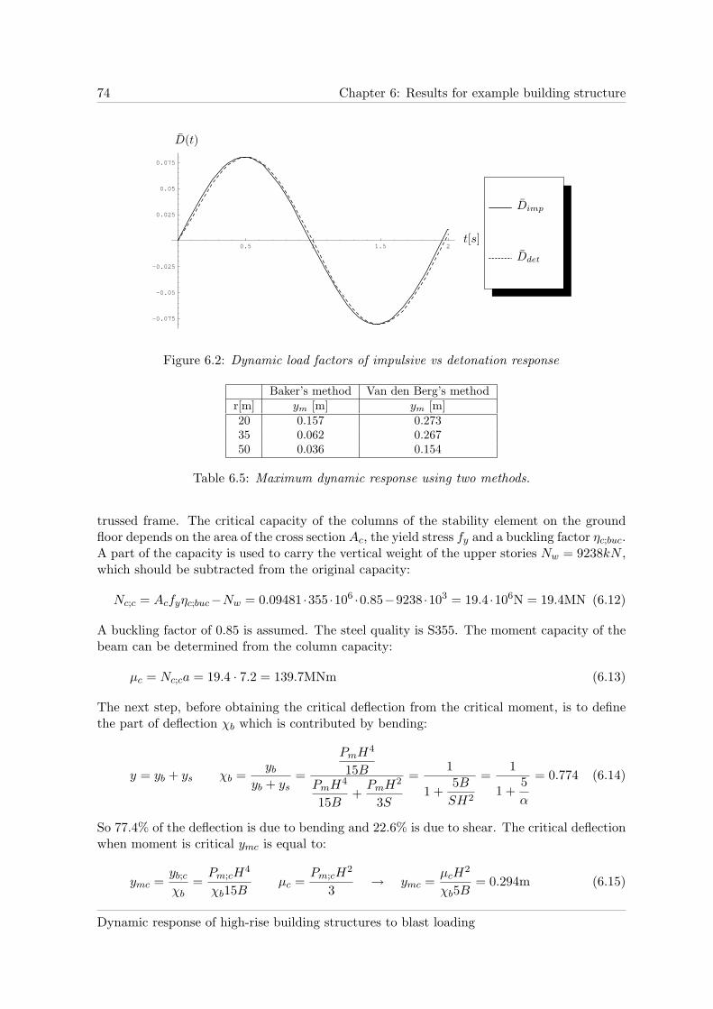
74 Chapter 6: Results for example building structure
0.5 1 1.5 2
-0.075
-0.05
-0.025
0.025
0.05
0.075
t[s]
D(t)
Dimp
Ddet
Figure 6.2: Dynamic load factors of impulsive vs detonation response
Baker’s method Van den Berg’s methodr[m] ym [m] ym [m]20 0.157 0.27335 0.062 0.26750 0.036 0.154
Table 6.5: Maximum dynamic response using two methods.
trussed frame. The critical capacity of the columns of the stability element on the groundfloor depends on the area of the cross section Ac, the yield stress fy and a buckling factor ηc;buc.A part of the capacity is used to carry the vertical weight of the upper stories Nw = 9238kN ,which should be subtracted from the original capacity:
Nc;c = Acfyηc;buc−Nw = 0.09481 ·355 ·106 ·0.85−9238 ·103 = 19.4 ·106N = 19.4MN (6.12)
A buckling factor of 0.85 is assumed. The steel quality is S355. The moment capacity of thebeam can be determined from the column capacity:
µc = Nc;ca = 19.4 · 7.2 = 139.7MNm (6.13)
The next step, before obtaining the critical deflection from the critical moment, is to definethe part of deflection χb which is contributed by bending:
y = yb + ys χb =yb
yb + ys=
PmH4
15BPmH4
15B+
PmH2
3S
=1
1 +5B
SH2
=1
1 +5
α
= 0.774 (6.14)
So 77.4% of the deflection is due to bending and 22.6% is due to shear. The critical deflectionwhen moment is critical ymc is equal to:
ymc =yb;c
χb=
Pm;cH4
χb15Bµc =
Pm;cH2
3→ ymc =
µcH2
χb5B= 0.294m (6.15)
Dynamic response of high-rise building structures to blast loading

6.3 Single degree of freedom response 75
The similar procedure can be followed for critical deflection when shear is critical ysc. Thediagonals have no initial load. It is assumed that wind loading which might be present duringthe blast loading, does not have a significant influence. In design practice it is safer to assumean average static wind load to be present during the blast loading. For now this is ignored.
Nd;c = Adfyηd;buc = 0.01414 · 355 · 106 · 0.85 = 4.27MN (6.16)
The critical shear force in the diagonal at ground level can be obtained from Nd;c:
vc =Nd;ca
d=
4.27 · 106 · 7.2
5.09= 6.04MN (6.17)
If χs = 0.226 is the part of the deflection due to shear, the critical shear deflection ysc can beobtained:
ysc =ys;c
χs=
Pm;cH2
χs3Svc = PmH → ysc =
vcH
χs3S= 0.275m (6.18)
The critical shear deflection is lower than the critical bending deflection, therefore sheardeflection is normative. Using Van den Berg’s method, it appears that 20m is the criticalrange for the example building with regard to failure due to overall response. This is withoutany safety factors, so in design practice, the diagonals should be over-dimensioned to gainmore shear capacity.
6.3.1 Pressure-impulse diagram for SDOF response
To make the pressure-impulse diagram useful as a design tool, it can be specialized for abuilding. The p − i−diagram in figure 4.12 has asymptotes Fm = 1/2 and I = 1, which canbe transformed to dimensional asymptotes:
Fm =Fm
Rc=
1
2→ Fm =
Rc
2(6.19)
I = Fmtd2
=Fm
Rc
ω1td2
=Iω1
Rc= 1 → I =
Rc
ω1(6.20)
To obtain the asymptotes, Rmc = Kymc and Rsc = Kysc can be substituted.
Rmc =Nc;caH2
5B
K
χbRsc =
Nd;caH
3dS
K
χs(6.21)
The fractions K/χb and K/χs can be simplified because
K
χb=
PmH
ys + yb
yb + ys
yb=
PmH
yb=
15B
H3= Kb (6.22)
and similarly
K
χs= Ks =
3S
H(6.23)
Substituting in Rmc and Rsc leads to:
Rmc =3Nc;ca
H= 6.47MN Rsc =
Nd;ca
d= 6.04MN (6.24)
L. J. van der Meer
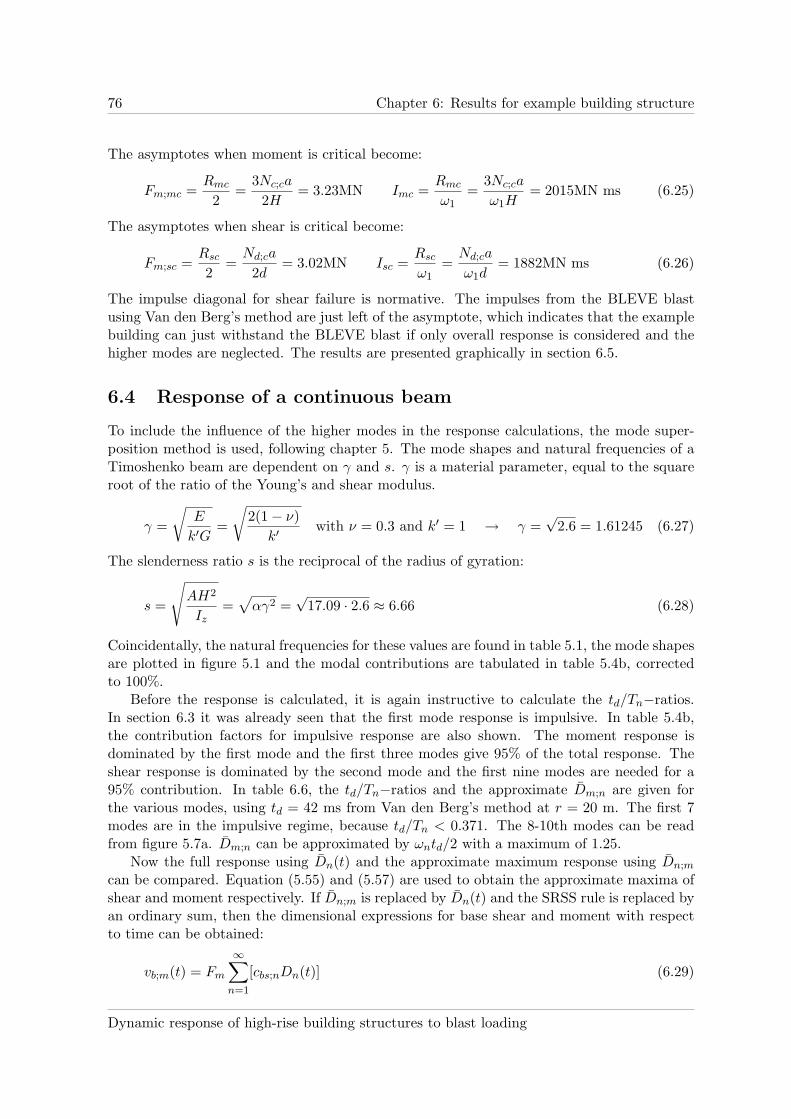
76 Chapter 6: Results for example building structure
The asymptotes when moment is critical become:
Fm;mc =Rmc
2=
3Nc;ca
2H= 3.23MN Imc =
Rmc
ω1=
3Nc;ca
ω1H= 2015MN ms (6.25)
The asymptotes when shear is critical become:
Fm;sc =Rsc
2=
Nd;ca
2d= 3.02MN Isc =
Rsc
ω1=
Nd;ca
ω1d= 1882MN ms (6.26)
The impulse diagonal for shear failure is normative. The impulses from the BLEVE blastusing Van den Berg’s method are just left of the asymptote, which indicates that the examplebuilding can just withstand the BLEVE blast if only overall response is considered and thehigher modes are neglected. The results are presented graphically in section 6.5.
6.4 Response of a continuous beam
To include the influence of the higher modes in the response calculations, the mode super-position method is used, following chapter 5. The mode shapes and natural frequencies of aTimoshenko beam are dependent on γ and s. γ is a material parameter, equal to the squareroot of the ratio of the Young’s and shear modulus.
γ =
√
E
k′G=
√
2(1 − ν)
k′with ν = 0.3 and k′ = 1 → γ =
√2.6 = 1.61245 (6.27)
The slenderness ratio s is the reciprocal of the radius of gyration:
s =
√
AH2
Iz=
√
αγ2 =√
17.09 · 2.6 ≈ 6.66 (6.28)
Coincidentally, the natural frequencies for these values are found in table 5.1, the mode shapesare plotted in figure 5.1 and the modal contributions are tabulated in table 5.4b, correctedto 100%.
Before the response is calculated, it is again instructive to calculate the td/Tn−ratios.In section 6.3 it was already seen that the first mode response is impulsive. In table 5.4b,the contribution factors for impulsive response are also shown. The moment response isdominated by the first mode and the first three modes give 95% of the total response. Theshear response is dominated by the second mode and the first nine modes are needed for a95% contribution. In table 6.6, the td/Tn−ratios and the approximate Dm;n are given forthe various modes, using td = 42 ms from Van den Berg’s method at r = 20 m. The first 7modes are in the impulsive regime, because td/Tn < 0.371. The 8-10th modes can be readfrom figure 5.7a. Dm;n can be approximated by ωntd/2 with a maximum of 1.25.
Now the full response using Dn(t) and the approximate maximum response using Dn;m
can be compared. Equation (5.55) and (5.57) are used to obtain the approximate maxima ofshear and moment respectively. If Dn;m is replaced by Dn(t) and the SRSS rule is replaced byan ordinary sum, then the dimensional expressions for base shear and moment with respectto time can be obtained:
vb;m(t) = Fm
∞∑
n=1
[cbs;nDn(t)] (6.29)
Dynamic response of high-rise building structures to blast loading

6.4 Response of a continuous beam 77
Mode ωn fn Tn td/Tn Dm;n
1 2.89 0.46 2.17 0.02 0.062 11.06 1.76 0.57 0.07 0.233 23.19 3.69 0.27 0.16 0.494 30.04 4.78 0.21 0.20 0.635 39.00 6.21 0.16 0.26 0.826 42.53 6.77 0.15 0.28 0.897 53.31 8.48 0.12 0.36 1.128 57.97 9.23 0.11 0.39 1.209 66.93 10.65 0.09 0.45 1.2010 74.72 11.89 0.08 0.50 1.20
Table 6.6: td/Tn− ratio and approximate DLF for 10 modes.
µb;m(t) =FmH
3
∞∑
n=1
[cbm;nDn(t)] (6.30)
The results are shown in figure 6.3 and compared to two approximation rules, namely theabsolute sum rule (abssum) and the square-root-of-sum-of-squares rule (srss). The SRSS ruleis developed for earthquake engineering and based on random vibration theory, as mentionedbefore. It seems that the SRSS rule is non-conservative for blast loading. The ABSSUM ruleis too conservative. In this particular case, the first maximum can be accurately approximatedby 1.5 times the SRSS rule. The first maximum is defined as the highest maximum in thefirst half of the first period of the first mode. Maxima that occur later are assumed to bereduced by damping, because the higher modes are affected more by damping than the firstmode.
6.4.1 Pressure-impulse diagram including higher modes
The asymptotes of the pressure-impulse diagram including higher modes are obtained byfollowing section 5.5. First the asymptotes when moment is normative:
Fm;mc =1
1.5· 3µc
2H
√
∞∑
n=1(cbm;n)2
=1
1.5· 3 · 139.7 · 106
2 · 64.8 · 0.825835= 2.61MN (6.31)
Imc =1
1.5· 3µc
H
√
∞∑
n=1(ωncbm;n)2
=1
1.5· 3 · 139.7 · 106
64.8 · 3.11413= 1385MNms (6.32)
The asymptotes when shear is normative are:
Fm;sc =1
1.5· vc
2
√
∞∑
n=1(cbs;n)2
=1
1.5· 6.04 · 106
2 · 0.518518= 3.88MN (6.33)
L. J. van der Meer

78 Chapter 6: Results for example building structure
Isc =1
1.5· vc√
∞∑
n=1(ωncbs;n)2
=1
1.5· 6.04 · 106
5.36292= 751MNms (6.34)
6.5 Comparison of results
For an example BLEVE blast loading on an example building the response and pressure-impulse diagram were obtained, using both a SDOF and a MDOF approach. In this section,the top displacement, base moment and base shear response are compared. Subsequently,the asymptotes of the pressure-impulse diagrams of SDOF and MDOF response are given,including the locations in the diagram of the BLEVE blasts at different ranges according toBaker’s and Van den Berg’s method. Finally, modification factors for the asymptotes of theSDOF p − i−diagram are given to include the influence of higher modes on the response.
6.5.1 Comparison of response
The influence of the higher modes is least significant in the top displacement, see figure 6.4a.More influence of higher modes is visible in the base moment, see figure 6.4b, and the baseshear has the highest contribution from the higher modes, see figure 6.4c.
6.5.2 Comparison of p − i− diagram
The p− i−diagram for the example BLEVE blast on the example building is shown in figure6.5. The SDOF p − i−diagram is non-conservative for impulsive response. The quasi-staticasymptotes are approximately equal for both failure criteria and SDOF and MDOF. It canbe concluded that the response to BLEVE blast loading is impulsive, because the impulsiveasymptotes are normative for determination of failure. The value of peak force from theBLEVE blast does not play a role in this. Shear is the likely type of failure, which can beexplained by the higher contribution factors of higher modes, compared to moment. Of coursethis is dependent on the dimensions of the columns and the diagonals in the trussed frame,which determine the moment and shear capacity. However, the columns and diagonals werealready dimensioned for wind loading, so their relative dimensions are realistic.
6.5.3 Modification factors for inclusion of higher modes
Pressure-impulse asymptotes for SDOF systems can be obtained easily. To include the in-fluence of higher modes, a modification factor for the asymptote would be useful, if it wereindependent of the failure criterium. The asymptotes of the SDOF diagram are found inequations (6.19)-(6.20):
Fm;sdof =Rc
Dm;qsIsdof =
Rc
ω1(6.35)
in which Dm;qs is the quasi-static dynamic load factor, equal to 2 for an idealized detonationand equal to 1 for an idealized deflagration.
Dynamic response of high-rise building structures to blast loading

6.5 Comparison of results 79
The asymptotes of the MDOF diagram are given in equations (6.31)-(6.34). Denotingthe correction factor 1.5 as ε, substituting Rc for µc and vc and generalizing the contributionfactor of the nth mode to cn, the asymptotes are obtained independent of the failure type:
Fm;mdof =Rc
εDm;qs
√
∞∑
n=1(cn)2
Imdof =Rc
ε
√
∞∑
n=1(ωncn)2
(6.36)
The modification factor λ of the asymptotes is defined as:
λqs =Fm;mdof
Fm;sdof=
1
ε
√
∞∑
n=1(cn)2
λi =Imdof
Isdof=
1
ε
√
∞∑
n=1(ωncn)2
with ωn =ωn
ω1(6.37)
So the modification factor λqs for the quasi-static asymptote is the reciprocal of the SRSSrule applied to the contribution factors cn and multiplied by a correction factor ε. Theimpulsive asymptote depends also on the ratio of ωn and ω1 for every n. The definition of λi
makes clear how important the higher modes are, because ωn keeps increasing with increasingn. So cn should relatively decrease more than ωn increases to decrease the influence of thehigher modes. This is only true for impulsive behavior of all modes, which is a limit case.Unless the load is a purely theoretical impulse, there are always high modes that have adynamic load factor Dm;n < ωntd/2, which reduces the influence of these modes, because ωn
disappears from the modal contribution. Dm;n ≈ 1.25 for modes with ωntd > 2.33112 for anidealized detonation. For an idealized deflagration, Dm;n for modes with ωntd > π should bedetermined with figure 5.8 for the td/Tn−value of each mode.
L. J. van der Meer

80 Chapter 6: Results for example building structure
1 2 3 4
-2´107
-1´107
1´107
2´107
t [s]
vb(t) [N]
vb(t) [N]
abssum
abssum
srss
srss
1.5×srss
1.5×srss
(a) Base shear
1 2 3 4
-2´108
-1´108
1´108
2´108
µb(t) [Nm]
µb(t) [Nm]
t [s]
abssum
abssum
srss
srss
1.5×srss
1.5×srss
(b) Base moment
Figure 6.3: Base shear and moment for 10 modes of continuous Timoshenko beam.
Dynamic response of high-rise building structures to blast loading
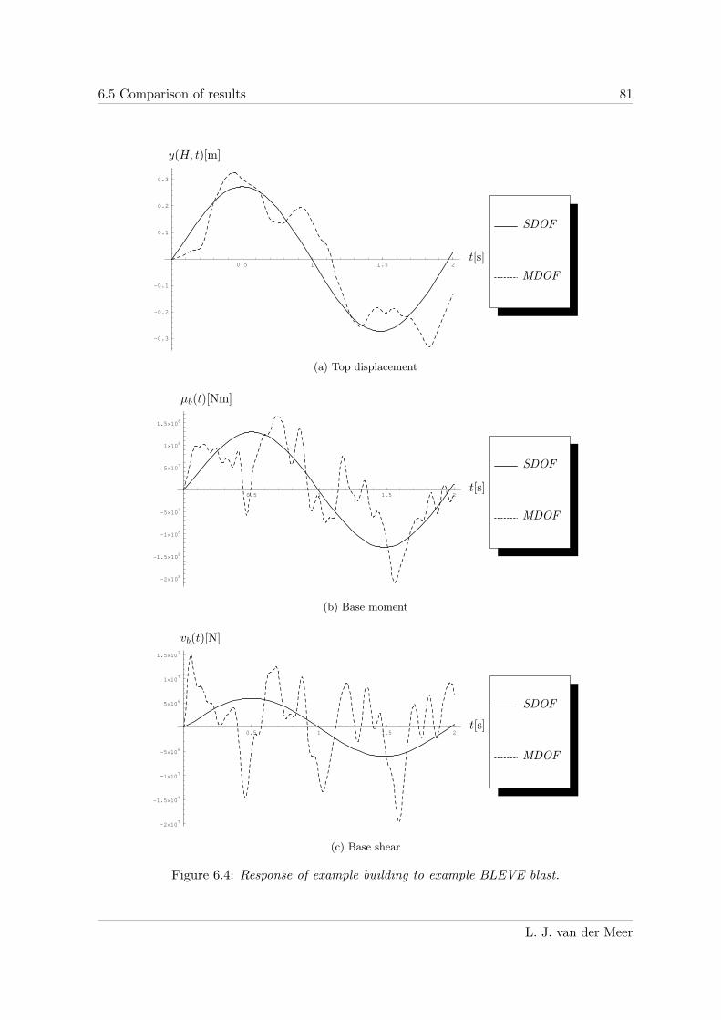
6.5 Comparison of results 81
0.5 1 1.5 2
-0.3
-0.2
-0.1
0.1
0.2
0.3
y(H, t)[m]
t[s]
SDOF
MDOF
(a) Top displacement
0.5 1 1.5 2
-2´108
-1.5´108
-1´108
-5´107
5´107
1´108
1.5´108
µb(t)[Nm]
t[s]
SDOF
MDOF
(b) Base moment
0.5 1 1.5 2
-2´107
-1.5´107
-1´107
-5´106
5´106
1´107
1.5´107
vb(t)[N]
t[s]
SDOF
MDOF
(c) Base shear
Figure 6.4: Response of example building to example BLEVE blast.
L. J. van der Meer
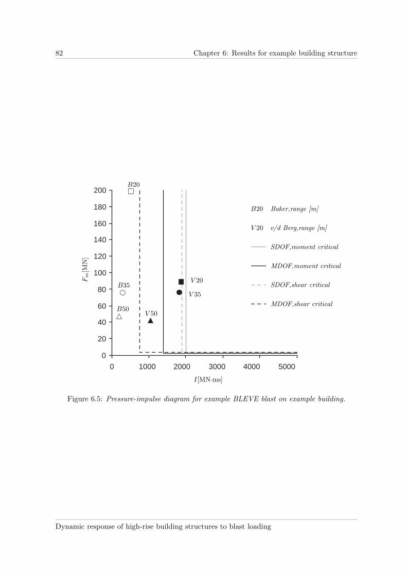
82 Chapter 6: Results for example building structure
0
20
40
60
80
100
120
140
160
180
200
0 1000 2000 3000 4000 5000
B20
B20
B35
B50
V 20
V 20
V 35
V 50
Fm
[MN
]
I[MN·ms]
Baker,range [m]
v/d Berg,range [m]
SDOF,moment critical
MDOF,moment critical
SDOF,shear critical
MDOF,shear critical
Figure 6.5: Pressure-impulse diagram for example BLEVE blast on example building.
Dynamic response of high-rise building structures to blast loading
83
Chapter 7
Conclusions
• Conclusions regarding BLEVE blast:
– BLEVE blast parameters according to Baker’s method result in too short positivephase durations, which is not conservative.
– BLEVE blast parameters according to Van den Berg’s method are preferred tothose according to Baker’s method, but modification factors for elevation and tankshape are not included.
• Conclusions regarding modeling:
– A trussed frame can be modeled as an equivalent beam, if it is assumed thatthe columns determine the bending stiffness and the diagonals determine the shearstiffness. The approximation is more accurate if the trussed frame has more stories.
– A continuous beam can be modeled as a single degree of freedom (SDOF) system,if it is assumed that only the first mode contributes to the response. The equivalentSDOF system should be energy equivalent to the beam in the first mode.
– Load-mass factors in literature apply only to slender beams. Trussed frame equiv-alent beams are generally non-slender.
– Load-mass factors can be determined for non-slender beams with or without arotary spring at the base using energy equivalence.
– Load-mass factors for a static deflected shape do not always result in an accuratefirst natural frequency. The first mode of vibration is better approximated by thestatic deflected shape for a uniform distributed load than for a linear or quadraticdistributed load.
• Conclusions regarding SDOF response:
– Impulsive response is independent of the blast pressure-time profile.
– The limit of quasi-static response to all decaying blast loads (starting with themaximum load) is determined by the response to a step function with a dynamicload factor equal to 2.
– The limit of quasi-static response to all rising blast loads (which reach a maximumafter some time) is determined by the static response with a dynamic load factorequal to 1.
L. J. van der Meer

84 Chapter 7: Conclusions
– Full transient response analysis is only necessary if the response is not in theimpulsive nor in the quasi-static regime.
– Pressure-impulse diagrams can be constructed numerically or analytically for anySDOF system including damping, non-linear material behavior and complicatedpressure-time profiles.
• Conclusions regarding response of a continuous Timoshenko beam:
– The trussed frame equivalent continuous beam can be modeled by a Timoshenkobeam, which includes shear deformation and rotary inertia.
– The mode shapes and natural frequencies of a Timoshenko beam can be determinednumerically.
– The mode shapes of a Timoshenko beam depend on the slenderness ratio (geomet-rical property) and on the ratio of the Young’s modulus and the shear modulus(material property).
– The force and the response can be written as a sum of modal forces and responses,which share the same time solution.
– Modal contribution factors for base shear and base moment can be defined, whichsum up to 1. Base shear contribution factors are always positive. Base momentcontribution factors can be positive or negative.
– For uniform, linear and quadratic load distribution, only two or three modes areneeded to have a minimum of 95% contribution to base moment.
– For 95% contribution to base shear, more modes are needed than for base moment.Least modes are needed for the uniform load distribution, more modes are neededfor the linear load distribution and most modes for the quadratic load distribution.
– The dynamic load factor for higher modes is dependent on the response regime ofthe mode with the highest contribution factor, usually the first mode.
– The maximum response including higher modes can be approximated by applyingthe SRSS rule to the peak values of modal response and multiplying the result bya factor. A conservative value for this factor has not been established.
– Impulsive and quasi-static response are obtained by assuming that all modes arein the impulsive and quasi-static regimes respectively.
– The contribution factors for quasi-static response cannot be used for impulsiveresponse, because the impulsive response depends on the product of natural fre-quency and contribution factor, resulting in more influence of the higher modes.
• Conclusions regarding example:
– The quasi-static response is similar for the SDOF system and the continuous beam.
– The impulsive response is underestimated by the SDOF system. The modificationfactor for the impulsive asymptote depends on the product of natural frequencyand contribution factor of all modes in the impulsive regime.
– The impulsive response is a limit case, assuming all modes are in the impulsiveregime. Depending on the td/T1−ratio, only a number of higher modes are in theimpulsive regime. Therefore the impulsive asymptote is conservative compared tothe actual p − i−diagram.
Dynamic response of high-rise building structures to blast loading

85
– If td = 100 ms and f1 = 1 Hz are taken as the most unfavorable combination of blastand structure, only the first two modes are in the impulsive regime. Nevertheless,the impulsive asymptote is reduced to 45% of the SDOF value. If td = 50 ms andf1 = 0.5 Hz, six modes are in the impulsive regime. In this case, the impulsiveasymptote is modified to approximately 35% of the SDOF value. If td/T1 ≈ 0.3,the SDOF and continuous response are approximately equal. Since td/T1 ≤ 0.1,BLEVE blast loading on high-rise building structures is in the impulsive regime.
– A SDOF system is non-conservative for BLEVE blast loading.
L. J. van der Meer


87
Chapter 8
Recommendations
• Recommendations regarding BLEVE blast loading:
– It should be investigated whether the correction factors in Baker’s method forelevation and shape of the tank agree with experiments of BLEVEs.
• Recommendations regarding response to blast loading:
– The influence of damping on the response of higher modes should be investigated.Modal damping can be added in the mode superposition method. Modal damp-ing ratios influence the dynamic load factors of the modes as well as the naturalfrequencies. However, for small damping, the damped natural frequencies canbe approximated by the undamped natural frequencies. The real challenge is toestimate the modal damping ratios. It is expected that higher mode vibrationsare damped sooner, because they have more oscillations in the same time periodcompared to the lower modes. Depending on how soon the maximum overall re-sponse is reach, damping has a certain influence on the response. If the maximumis reached soon, damping has little influence. If the maximum is reached rela-tively late, damping might have a considerable influence. Damping decreases theinfluence of higher modes, so ignoring it might be over-conservative.
– The influence of higher modes should be investigated in combination with non-linear material behavior. This is quite difficult, because the mode superpositionmethod cannot be used for non-linear material behavior. The non-linear mate-rial behavior occurs only locally, in a plastic hinge, so the question is how thedifferential equation of motion is affected by this.
– The influence of higher modes should be investigated in combination with otherpressure-time profiles. An important aspect is the inclusion of a large negativephase followed by a second shock, because these are associated with BLEVE blast.
– A better modal combination rule should be found for response to blast loading,which can replace the SRSS rule.
– A reliable method to determine the maximum of a sum of several harmonic func-tions is needed.
– The actual shape of a pressure-impulse diagram in the dynamic regime includinghigher modes should be determined numerically, to compare it with the asymptotes.The impulsive asymptote might be too conservative.
L. J. van der Meer

88 Chapter 8: Recommendations
– The influence of failing building elements on the overall response should be inves-tigated. In this report, it was assumed that all load on the facade is transferred tothe bearing structure.
– The response of a high-rise building structure should be determined numericallyfor a sequential load, which arrives first at the base at the front and later at thetop and sides. In this report, it was assumed that the blast arrived at the sametime at every location on the front facade. Both responses should be compared.
• Recommendations regarding modeling:
– Mode shapes and natural frequencies should be calculated for sandwich beams,which represent most types of stability elements. In addition it should be possibleto include varying cross-section, bending stiffness, shear stiffness and mass.
– Mode shapes and natural frequencies of continuous beams with base rotationshould be determined.
– Modal contribution factors for different beam types, slenderness ratios, materialparameters and load distributions should be tabulated.
Dynamic response of high-rise building structures to blast loading

89
Appendix A
Matlab input files
A.1 Pressure-impulse diagram (SDOF)
The determination of the p − i−diagam consists of two parts:
• Definition of a forcing function.
• The main file where the diagram is determined.
The main file is shown below:
clear all
close all
clc
TD = [];
TM = [];
P = [];
IMPULSE = [];
YP = [];
tau_step = 5e-3;
tau1_step = 5e-3;
step_td = 1e-4;
count = 0;
TD = 0.2:.2:50;
for td = TD;
t2 = 0:td.*step_td:td;
Load2 = force(t2,td);
[value_max index_max] = max(Load2);
t2m = t2(index_max);
CONV = [];
TAU = [];
stop = 0;
tau = 0;
while stop == 0;
tau1 = 0:tau1_step:tau;
Conv = sum(force(tau1,td).*sin(tau-tau1).*tau1_step);
TAU = [TAU, tau];
CONV = [CONV, Conv];
tau = tau + tau_step;
if tau > t2m & tau > tau_step;
L. J. van der Meer

90 Chapter A: Matlab input files
if CONV(end) < CONV(end-1);
stop =1;
end
end
end
plot(TAU,CONV,’k-’)
hold on
xlabel(’t’)
ylabel(’y’)
grid on
drawnow
[value1_max index1_max] = max(CONV);
tm = TAU(index1_max);
TM = [TM, tm];
p = 1./value1_max;
IntF = sum(Load2.*td.*step_td);
Impulse = IntF.*p;
P = [P, p];
IMPULSE = [IMPULSE, Impulse];
count = count + 1
end
figure
plot(IMPULSE,P,’k-o’)
axis([0 max(IMPULSE) 0 max(P)])
grid on
xlabel(’i’)
ylabel(’p’)
figure
plot(TD,1./P,’k-o’)
grid on
xlabel(’wtd’)
ylabel(’ymaxp’)
figure
plot(TD,TM./TD,’k-o’)
grid on
xlabel(’td’)
ylabel(’tmtd’)
TD_def = TD;
TM_def = TM;
P_def = P;
IMPULSE_def = IMPULSE;
YP_def = YP;
% TD_det = TD;
% TM_det = TM;
% P_det = P;
% IMPULSE_det = IMPULSE;
% YP_det = YP;
save def.mat TD_def TM_def P_def IMPULSE_def YP_def
% save det.mat TD_det TM_det P_det IMPULSE_det YP_det
The forcing function for an idealized deflagration is:
function [out] = force(t,td);
if min(t) < 0
Dynamic response of high-rise building structures to blast loading

A.2 Wave numbers of a Timoshenko beam 91
sprintf(’t < 0 not possible!’)
pause
end
for i = 1:length(t)
if t(i) <= td/2
out(i) = 2*t(i)./td;
elseif t(i) <= td & t(i) > td/2
out(i) = 2-2*t(i)./td;
elseif t(i) > td
out(i) = 0;
end
end
The forcing function for an idealized detonation is:
function [out] = force(t,td);
if min(t) < 0
sprintf(’t < 0 not possible!’)
pause
end
for i = 1:length(t)
if t(i) <= td
out(i) = 1-t(i)./td;
elseif t(i) > td
out(i) = 0;
end
end
A.2 Wave numbers of a Timoshenko beam
The determination of the wave numbers consists of two parts:
• Definition of a frequency equation (5.9).
• The main file where the wave numbers are determined.
The main file is shown below:
clear all
close all
clc
global s g
RECALC = 1;
S = 6.6635
G = 1.61245
N = 10;
if RECALC == 1;
ac = s*sqrt(1/g^2+1);
x0 = 1;
[a_n,fval,exitflag] = fzero(@Timoshenko_function,x0);
a(1) = a_n; x = a_n;
b(1) = 1/sqrt(2*g^2) .* sqrt(-x.^2*(1+g^4)+...
(1+g^2)*( -s^2 + sqrt(x.^4.*(-1+g^2)^2+2*x.^2.*(1+g^2)*s^2+s^4) ));
if x >= ac
b(1) = 1/sqrt(2*g^2) .* sqrt(x.^2*(1+g^4)-...
(1+g^2)*( -s^2 + sqrt(x.^4.*(-1+g^2)^2+2*x.^2.*(1+g^2)*s^2+s^4) ));
L. J. van der Meer
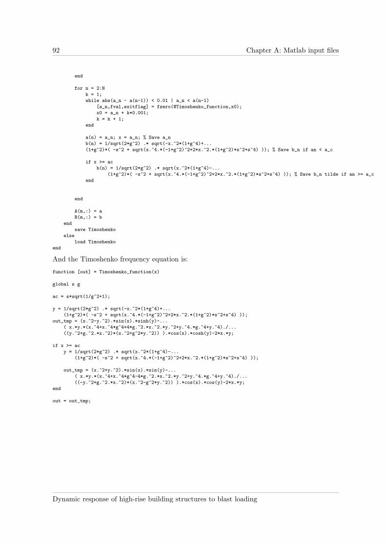
92 Chapter A: Matlab input files
end
for n = 2:N
k = 1;
while abs(a_n - a(n-1)) < 0.01 | a_n < a(n-1)
[a_n,fval,exitflag] = fzero(@Timoshenko_function,x0);
x0 = a_n + k*0.001;
k = k + 1;
end
a(n) = a_n; x = a_n; % Save a_n
b(n) = 1/sqrt(2*g^2) .* sqrt(-x.^2*(1+g^4)+...
(1+g^2)*( -s^2 + sqrt(x.^4.*(-1+g^2)^2+2*x.^2.*(1+g^2)*s^2+s^4) )); % Save b_n if an < a_c
if x >= ac
b(n) = 1/sqrt(2*g^2) .* sqrt(x.^2*(1+g^4)-...
(1+g^2)*( -s^2 + sqrt(x.^4.*(-1+g^2)^2+2*x.^2.*(1+g^2)*s^2+s^4) )); % Save b_n tilde if an >= a_c
end
end
A(m,:) = a
B(m,:) = b
end
save Timoshenko
else
load Timoshenko
end
And the Timoshenko frequency equation is:
function [out] = Timoshenko_function(x)
global s g
ac = s*sqrt(1/g^2+1);
y = 1/sqrt(2*g^2) .* sqrt(-x.^2*(1+g^4)+...
(1+g^2)*( -s^2 + sqrt(x.^4.*(-1+g^2)^2+2*x.^2.*(1+g^2)*s^2+s^4) ));
out_tmp = (x.^2-y.^2).*sin(x).*sinh(y)-...
( x.*y.*(x.^4+x.^4*g^4+4*g.^2.*x.^2.*y.^2+y.^4.*g.^4+y.^4)./...
((y.^2+g.^2.*x.^2)*(x.^2+g^2*y.^2)) ).*cos(x).*cosh(y)-2*x.*y;
if x >= ac
y = 1/sqrt(2*g^2) .* sqrt(x.^2*(1+g^4)-...
(1+g^2)*( -s^2 + sqrt(x.^4.*(-1+g^2)^2+2*x.^2.*(1+g^2)*s^2+s^4) ));
out_tmp = (x.^2+y.^2).*sin(x).*sin(y)-...
( x.*y.*(x.^4+x.^4*g^4-4*g.^2.*x.^2.*y.^2+y.^4.*g.^4+y.^4)./...
((-y.^2+g.^2.*x.^2)*(x.^2-g^2*y.^2)) ).*cos(x).*cos(y)-2*x.*y;
end
out = out_tmp;
Dynamic response of high-rise building structures to blast loading

93
Appendix B
Ansys input files
The Ansys input files consist of three models:
• A trussed frame model with lumped mass.
• An equivalent beam model with lumped mass.
• An equivalent beam model with distributed mass.
Two types of analysis are done:
• Static analysis for wind loading.
• Modal analysis to determine natural frequencies and mode shapes.
First the trussed frame model with lumped mass:
/PREP7
ET,1,LINK1 !link elements, tension/compression, no bending
ET,2,MASS21,,,4 !mass elements
!ET,3,COMBIN14,0,2, !spring elements, for rotation of foundation
R,1,0.09481, !column, HD 400x744
R,2,0.01414, !diagonal, HF RHS 300x300x12.5
R,3,100 !beam, ’infinitely’ stiff
R,4,114400.8 !mass
!R,5,2.099E09 !translational spring stiffness
MP,EX,1,2.1E11 !steel Young’s modulus
MP,PRXY,1,0.30 !steel Poisson ratio
N,1,-3.6,0 !nodes left side
N,2,-3.6,3.6
N,3,-3.6,7.2
N,4,-3.6,10.8
N,5,-3.6,14.4
N,6,-3.6,18
N,7,-3.6,21.6
N,8,-3.6,25.2
N,9,-3.6,28.8
N,10,-3.6,32.4
N,11,-3.6,36
N,12,-3.6,39.6
N,13,-3.6,43.2
N,14,-3.6,46.8
L. J. van der Meer

94 Chapter B: Ansys input files
N,15,-3.6,50.4
N,16,-3.6,54
N,17,-3.6,57.6
N,18,-3.6,61.2
N,19,-3.6,64.8
N,20,3.6,0 !nodes right side
N,21,3.6,3.6
N,22,3.6,7.2
N,23,3.6,10.8
N,24,3.6,14.4
N,25,3.6,18
N,26,3.6,21.6
N,27,3.6,25.2
N,28,3.6,28.8
N,29,3.6,32.4
N,30,3.6,36
N,31,3.6,39.6
N,32,3.6,43.2
N,33,3.6,46.8
N,34,3.6,50.4
N,35,3.6,54
N,36,3.6,57.6
N,37,3.6,61.2
N,38,3.6,64.8
N,39,0,3.6 !nodes middle
N,40,0,7.2
N,41,0,10.8
N,42,0,14.4
N,43,0,18
N,44,0,21.6
N,45,0,25.2
N,46,0,28.8
N,47,0,32.4
N,48,0,36
N,49,0,39.6
N,50,0,43.2
N,51,0,46.8
N,52,0,50.4
N,53,0,54
N,54,0,57.6
N,55,0,61.2
N,56,0,64.8
!N,57,-3.6,0 !nodes for translational springs
!N,58,3.6,0
REAL,1 !column
TYPE,1 !link element
E,1,2
E,2,3
E,3,4
E,4,5
E,5,6
E,6,7
E,7,8
E,8,9
E,9,10
E,10,11
E,11,12
E,12,13
E,13,14
E,14,15
E,15,16
Dynamic response of high-rise building structures to blast loading

95
E,16,17
E,17,18
E,18,19
E,20,21
E,21,22
E,22,23
E,23,24
E,24,25
E,25,26
E,26,27
E,27,28
E,28,29
E,29,30
E,30,31
E,31,32
E,32,33
E,33,34
E,34,35
E,35,36
E,36,37
E,37,38
REAL,3 !beam
TYPE,1 !link element
E,1,20
E,2,39
E,39,21
E,3,40
E,40,22
E,4,41
E,41,23
E,5,42
E,42,24
E,6,43
E,43,25
E,7,44
E,44,26
E,8,45
E,45,27
E,9,46
E,46,28
E,10,47
E,47,29
E,11,48
E,48,30
E,12,49
E,49,31
E,13,50
E,50,32
E,14,51
E,51,33
E,15,52
E,52,34
E,16,53
E,53,35
E,17,54
E,54,36
E,18,55
E,55,37
E,19,56
E,56,38
REAL,2 !diagonal
TYPE,1 !link element
L. J. van der Meer

96 Chapter B: Ansys input files
E,1,39
E,20,39
E,2,40
E,21,40
E,3,41
E,22,41
E,4,42
E,23,42
E,5,43
E,24,43
E,6,44
E,25,44
E,7,45
E,26,45
E,8,46
E,27,46
E,9,47
E,28,47
E,10,48
E,29,48
E,11,49
E,30,49
E,12,50
E,31,50
E,13,51
E,32,51
E,14,52
E,33,52
E,15,53
E,34,53
E,16,54
E,35,54
E,17,55
E,36,55
E,18,56
E,37,56
!REAL,5 !translational spring stiffness
!TYPE,3 !translational spring element
!E,57,1
!E,58,20
REAL,4 !lumped mass
TYPE,2 !mass element
E,39 !mass is applied to nodes in the middle
E,40
E,41
E,42
E,43
E,44
E,45
E,46
E,47
E,48
E,49
E,50
E,51
E,52
E,53
E,54
E,55
E,56
Dynamic response of high-rise building structures to blast loading

97
!D,57,UX !extra constraints if translational spring is present
!D,57,UY
!D,58,UX
!D,58,UY
D,1,UX !constraints
D,1,UY
D,20,UX
D,20,UY
D,39,UY !vertical constraint of mass elements
D,40,UY
D,41,UY
D,42,UY
D,43,UY
D,44,UY
D,45,UY
D,46,UY
D,47,UY
D,48,UY
D,49,UY
D,50,UY
D,51,UY
D,52,UY
D,53,UY
D,54,UY
D,55,UY
D,56,UY
F,19,FX,19050 !lumped forces for wind deflection
F,18,FX,38099
F,17,FX,38099
F,16,FX,38099
F,15,FX,38099
F,14,FX,38099
F,13,FX,38099
F,12,FX,38099
F,11,FX,38099
F,10,FX,38099
F,9,FX,38099
F,8,FX,38099
F,7,FX,38099
F,6,FX,38099
F,5,FX,38099
F,4,FX,38099
F,3,FX,38099
F,2,FX,38099
The input file for the equivalent beam with lumped mass:
/PREP7
ET,1,BEAM3 !beam element
ET,2,MASS21,,,4 !2D mass element without rotary inertia
!ET,3,COMBIN14,0,6 !rotational spring
R,1,0.02599,2.457,7.2,1 !area, area moment of inertia, height, include shear deflection
R,2,114400.8 !mass of mass element
!R,3,5.440608E10 !rotational spring stiffness
MP,EX,1,2.1E11 !steel Young’s modulus
MP,GXY,1,8.08E10 !steel Shear modulus
N,1,0,0 !nodes
N,2,0,3.6
N,3,0,7.2
N,4,0,10.8
N,5,0,14.4
L. J. van der Meer

98 Chapter B: Ansys input files
N,6,0,18
N,7,0,21.6
N,8,0,25.2
N,9,0,28.8
N,10,0,32.4
N,11,0,36
N,12,0,39.6
N,13,0,43.2
N,14,0,46.8
N,15,0,50.4
N,16,0,54
N,17,0,57.6
N,18,0,61.2
N,19,0,64.8
!N,20,0,0 !node for rotational spring
TYPE,1 !beam element
REAL,1 !beam constants
E,1,2
E,2,3
E,3,4
E,4,5
E,5,6
E,6,7
E,7,8
E,8,9
E,9,10
E,10,11
E,11,12
E,12,13
E,13,14
E,14,15
E,15,16
E,16,17
E,17,18
E,18,19
TYPE,2 !mass element
REAL,2 !lumped mass
E,2
E,3
E,4
E,5
E,6
E,7
E,8
E,9
E,10
E,11
E,12
E,13
E,14
E,15
E,16
E,17
E,18
E,19
!TYPE,3 !rotational spring element
!REAL,3 !rotational spring stiffness
!E,20,1
Dynamic response of high-rise building structures to blast loading

99
!D,20,UX !extra constraints for rotational spring
!D,20,UY
!D,20,ROTZ
D,1,UX !constraints
D,1,UY
D,1,ROTZ
D,2,UY !vertical constraints for mass
D,3,UY
D,4,UY
D,5,UY
D,6,UY
D,7,UY
D,8,UY
D,9,UY
D,10,UY
D,11,UY
D,12,UY
D,13,UY
D,14,UY
D,15,UY
D,16,UY
D,17,UY
D,18,UY
D,19,UY
The forces are left out because they are similar to the previous input file. If the mass isdistributed, the lumped mass elements are left out and the beam element constants arereplaced by:
R,1,0.02599,2.457,7.2,1,,31778
Static analysis is done by adding the following strings to the input files:
/SOL
ANTYPE,0
SOLVE
FINISH
Modal analysis is done by adding the following string:
/SOL
ANTYPE,2
MODOPT,LANB,18,0,,,OFF
MXPAND,18, , ,0
SOLVE
FINISH
L. J. van der Meer

100
References
[1] Tasneem Abbasi and S. A. Abbasi. Bleve: mechanism, consequence assessment, man-agement. Journal of Hazardous Materials, 141:489–519, 2007.
[2] G. R. Abrahamson and H. E. Lindberg. Peak load-impulse characterization of criticalpulse loads in structural dynamics. Nuclear Engineering and Design, 37:35–46, January1976.
[3] US Army, Navy, and Air Force. Structures to resist the effect of accidental explosions.Technical report, Departments of the US Army, Navy and Air Force, 1990.
[4] J. M. Biggs. Introduction to Structural Dynamics. McGraw-Hill, 1964.
[5] A. M. Birk and M. H. Cunningham. The boiling liquid expanding vapor explosion.Journal of Loss Prevention in the Process Industries, 7(6):474–480, 1994.
[6] A. M. Birk, C. Davison, and M. Cunningham. Blast overpressures from medium scalebleve tests. Journal of Loss Prevention in the Process Industries, 20:194–206, 2007.
[7] A. K. Chopra. Dynamics of structures - Theory and applications to earthquake engineer-ing. Prentice Hall International Series in Civil Engineering and Engineering Mechanics.Prentice Hall, New Jersey, 1995.
[8] A. Soleiman Fallah and L. A. Louca. Pressure-impulse diagrams for elastic-plastic-hardening and softening single-degree-of-freedom models subjected to blast loading.Journal of Impact Engineering, 34:823–842, 2007.
[9] S. M. Han, H. Benaroya, and T. Wei. Dynamics of transversely vibrating beams usingfour engineering theories. Journal of Sound and Vibration, 225(5):935–988, 1999.
[10] J. C. D. Hoenderkamp. Hoge gebouwen, constructies voor stabiliteit. Technische Univer-siteit Eindhoven, 2004. Newer editions available in English.
[11] T. Krauthammer. Protecting critical infrastructure systems. Urban Habitat Construc-tions under Catastrophic Events, 2007. ISBN 978-80-01-03583-2.
[12] T. Krauthammer, S. Astarlioglu, J. Blasko, T. B. Soh, and P. H. Ng. Pressure-impulsediagrams for the behavior assessment of structural components. International Journalof Impact Engineering, 2007. Article in press.
[13] Q. M. Li and H. Meng. Pressure-impulse diagram for blast loads based on dimen-sional analysis and single-degree-of-freedom model. Journal of engineering mechanics,128(1):87–92, 2002.
Dynamic response of high-rise building structures to blast loading

REFERENCES 101
[14] Q. M. Li and H. Meng. Pulse loading shape effects on pressure-impulse diagram ofan elastic-plastic, single-degree-of-freedom structural model. International journal ofmechanical sciences, 44:1985–1998, 2002.
[15] Y. Lu and Z. Wang. Characterization of structural effects from above-ground explosionusing coupled numerical simulation. Computers and Structures, 84:1729–1742, 2006.
[16] G. W. Ma, H. J. Shi, and D. W. Shu. P-i diagram method for combined failure modesof rigid-plastic beams. Journal of Impact Engineering, 34:1081–1094, 2007.
[17] S. S. Rao. Mechanical Vibrations. Prentice Hall, Pearson Education, si edition, 2005.
[18] P. D. Smith. State of the art in europe and activity developed within wg3 impact andexplosion. Urban Habitat Constructions under Catastrophic Events, 2007. ISBN 978-80-01-03583-2.
[19] P. D. Smith and J. G. Hetherington. Blast and Ballistic Loading of Structures. ElsevierScience. Butterworth-Heinemann, Oxford, 1994.
[20] P. D. Smith and T. A. Rose. Blast wave propagation in city streets - an overview.Progress in structural engineering and materials, 8:16–28, 2006.
[21] A. C. van den Berg, M. M. van der Voort, J. Weerheijm, and N. H. A. Versloot.Expansion-controlled evaporation: a safe approach to bleve blast. Journal of loss pre-vention in the process industries, 17:397–405, 2004.
[22] VROM. Publicatiereeks gevaarlijke stoffen 1, deel 2b: Effecten van explosie op con-structies. Technical report, Ministerie van Binnenlandse Zaken en Koninkrijksrelaties,Ministerie van Verkeer en Waterstaat, 2003.
[23] VROM. Publicatiereeks gevaarlijke stoffen 2, methods for the calculation of physicaleffects due to releases of hazardous materials (liquids and gasses). Technical report,Ministerie van Binnenlandse Zaken en Koninkrijksrelaties, Ministerie van Verkeer enWaterstaat, 2005.
[24] F. Wald, F. Mazzolani, M. Byfield, D. Dubina, and M. Faber, editors. Urban habitatconstructions under catastrophic events, Proceedings of workshop Prague 30.-31.3.2007,Action C26. Czech Technical University, Prague, 2007.
L. J. van der Meer