dynamic response of highway bridge superstructures
TRANSCRIPT

Portland State University Portland State University
PDXScholar PDXScholar
Dissertations and Theses Dissertations and Theses
6-22-2020
Dynamic Response of Highway Bridge Dynamic Response of Highway Bridge
Superstructures Subjected to Wave Action: Superstructures Subjected to Wave Action:
Experimental Analysis and Numerical Modeling Experimental Analysis and Numerical Modeling
Alaa Waleed Hameed Portland State University
Follow this and additional works at: https://pdxscholar.library.pdx.edu/open_access_etds
Part of the Civil Engineering Commons
Let us know how access to this document benefits you.
Recommended Citation Recommended Citation Hameed, Alaa Waleed, "Dynamic Response of Highway Bridge Superstructures Subjected to Wave Action: Experimental Analysis and Numerical Modeling" (2020). Dissertations and Theses. Paper 5489. https://doi.org/10.15760/etd.7361
This Dissertation is brought to you for free and open access. It has been accepted for inclusion in Dissertations and Theses by an authorized administrator of PDXScholar. Please contact us if we can make this document more accessible: [email protected].

Dynamic Response of Highway Bridge Superstructures Subjected to Wave
Action: Experimental Analysis and Numerical Modeling
by
Alaa Waleed Hameed
A dissertation submitted in partial fulfillment of the requirements for the degree of
Doctor of Philosophy in
Civil and Environmental Engineering
Dissertation Committee: Thomas Schumacher, Chair
Arash Khosravifar Christopher Higgins
Minjie Zhu Hormoz Zareh
Portland State University 2020

i
Abstract
Bridges are critical lifeline components of the infrastructure network,
enabling economies to function under normal conditions and disaster response
and recovery missions to take place after extreme events. Therefore, ensuring
satisfactory performance increases community resilience and minimizes both
human and economic losses. Coastal bridges, which are the focus of this PhD
dissertation, are vulnerable to coastal storms. High failure rates of these bridges
during two major hurricane events in the mid-2000s have spurred research
activities to better understand the wave-induced forces of coastal bridges.
This PhD research represents a continuation effort to build, implement, and
introduce new fundamental concepts and methods that are important to the bridge
engineering community. The data set analyzed was part of an experimental study
conducted at the O. H. Hinsdale Wave Research Laboratory at Oregon State
University in 2007. A unique aspect of the setup was that the substructure flexibility
of the 1:5-scale bridge specimen could be adjusted by inserting springs with
different stiffnesses. The realistic specimen was subjected to a range of wave
conditions, water levels, and substructure fixity conditions.
First, a suitable equation of motion was developed as it represents an
essential building block for the any for any planned simulation effort. This equation
was derived based on the examination of the damping behavior of the system. This
effort lead to a better understanding of how the dynamic properties of the bridge
superstructure specimen are affected by different levels of submersion, and what
their numerical values are.

ii
Second, the available data set was analyzed in depth with the objective to
determine the effect of substructure flexibility on the observed wave-induced forces
on the bridge superstructure specimen. Reinforced by the test of restriction, it was
found that that the measured forces experienced by the superstructure specimen
with a flexible substructure were notably larger compared to the rigid case. These
findings highlight the need to account for substructure flexibility when estimating
wave forces. The proposed force magnification factors can be used in conjunction
with code equations that are based on rigid support conditions.
Finally, in order to expand the understanding of substructure flexibility and
exploring test conditions that are not part of the original experimental dataset,
having a numerical model is a promising solution. The particle finite element
method (PFEM) was selected as the tool for this purpose and is introduced and
evaluated against sample responses from the experiment.
In conclusion, support conditions affect the dynamic response of bridges
subjected to wave action and thus need to be considered. This PhD dissertation
created a better fundamental understanding of how bridges respond dynamically
to wave action considering varying levels of submersion as well as substructure
flexibility. The findings allow bridge engineers to build more accurate numerical
models for fluid-structure interaction problems and provide practical guidance with
respect to the magnification of wave-induced forces for design and evaluation
applications.

iii
Acknowledgments
I would like to express my gratefulness to Allah (The Merciful and most
Griseous, The provider) for his mercy and guidance, and surrounding me with
amazing people who had directly influenced me in my life journey in general and
during my PhD study in special. The only way of showing this gratefulness is by
thanking those people. Words will not be sufficient to express thanks, to…
… my parents, thanks for your genuine and continuous streaming of help and
love all lifelong, for your encouragement to continue my study abroad and for
your prayers.
… my husband and children, thanks for your presence and support during my
study, for your understanding, patience and sacrificing your needs to grant
me extra time to study.
… The Higher Committee for Education in Iraq (HCED), for sponsoring my study
in Portland State University for six years.
… my advisor (Dr. Thomas Schumacher), for providing me the data and sketches
present in this dissertation, trusting and patience, and his continuous advice,
help and support until the last minutes of preparing this dissertation.
… Dr. Zhu for his support and help in learning and implementing OpenSeesPy.
… Dr. Higgins for his valuable comments and assistance.

iv
Table of Contents
Abstract ................................................................................................................. i
Acknowledgments ................................................................................................ iii
List of Tables ........................................................................................................vi
List of Figures ...................................................................................................... vii
Chapter 1 .............................................................................................................. 1
Introduction ........................................................................................................... 1
1.1 Introduction ................................................................................................. 1
1.2 Dissertation Outline ..................................................................................... 4
1.3 References .................................................................................................. 8
Chapter 2 ............................................................................................................ 10
Manuscript 1: Characterization of Dynamic Properties from Free Vibration Tests of
a Large-Scale Bridge Model ............................................................................... 10
2.1 Introduction and Background .................................................................... 10
2.2 Motivation and Significance ....................................................................... 13
2.3 Experimental Test Setup and Free Vibration Tests ................................... 14
2.4 Initial Observations from Free Vibration Tests .......................................... 17
2.5 Analysis ..................................................................................................... 21
2.5.1 Numerical Model ................................................................................. 21
2.5.2 Parameter Estimation .......................................................................... 23
2.6 Quantification of Added Mass Parameters ................................................ 33
2.7 Summary and Conclusions ....................................................................... 36
2.8 References ................................................................................................ 38
Chapter 3 ............................................................................................................ 41
Manuscript 2: Effect of Substructure Flexibility on Wave-induced Forces on Bridge
Superstructures .................................................................................................. 41
3.1 Introduction and Background .................................................................... 41
3.2 Motivation and Objectives ......................................................................... 47
3.3 Experimental Setup ................................................................................... 48
3.4 Data Analysis ............................................................................................ 55
3.4.1 Unnormalized feature analysis ............................................................ 55

v
3.4.2 Normalized feature analysis ................................................................ 60
3.5 Substructure Flexibility Effect .................................................................... 63
3.6 Summary and Conclusion ......................................................................... 71
3.7 References ................................................................................................ 73
Chapter 4 ............................................................................................................ 75
Manuscript 3: Implementation of the OpenSeesPy Particle Finite Element Method
(PFEM) to Study Wave-induced Forces on Bridge Superstructures ................... 76
4.1 Introduction ............................................................................................... 75
4.2 Motivation and Objective ........................................................................... 77
4.3 Overview of the PFEM Method.................................................................. 78
4.4 Governing Equations ................................................................................. 79
4.5 Experimental Study ................................................................................... 81
4.6 Simulations ................................................................................................ 83
4.7 Model Validation and Results .................................................................... 86
4.8 Summary and Conclusions ....................................................................... 94
4.9 References ................................................................................................ 95
Chapter 5 ............................................................................................................ 99
Conclusions and Future Work .......................................................................... 100
5.1 Summary and Conclusions ....................................................................... 99
5.2 Recommendations for Future Work ......................................................... 101
Appendix A: Runge-Kutta Method .................................................................... 103
Appendix B: Global Search Algorithm Validation .............................................. 108
Appendix C: Parametric Study Exploring Effect of Damping Types on Response ......................................................................................................................... 110
Appendix D: Scatter Plots of Wave-Induced Forces vs. Wave Height .............. 118
Appendix E: Magnification Factors for all Cases .............................................. 119
Appendix F: Experiment -simulation results comparisons ................................ 122
Appendix G: Flexibility Effect via Experiment and Simulation Results .............. 123

vi
List of Tables
Table 2.1. Test matrix of free vibration tests. ...................................................... 16
Table 2.2. Natural vibration frequencies, fn for different test trials and phases obtained by DFT. ......................................................................................... 19
Table 2.3. Parameter estimates for all test trials obtained from the global search method. ........................................................................................................ 27
Table 2.4. Added mass factors and added mass coefficients calculated for both setups in fully submerged condition, 2a (= medium springs) and 2b (= soft springs)*. ...................................................................................................... 34
Table 2.5. Hydrodynamic mass per unit length for circular and rectangular sections. ....................................................................................................... 36
Table 3.1. Structural configurations and test phases investigated in [6] and used in this study. ..................................................................................................... 48
Table 3.2. Studied still water levels (SWL). ........................................................ 51
Table 3.3. Test of restrictions results. ................................................................. 67
Table 3.4. Force magnification factors at different percentiles, for both horizontal and vertical forces ........................................................................................ 70

vii
List of Figures
Figure 2.1. Elevation view of bridge superstructure model with key instrumentation used in this study (a) from the side and (b) looking down the flume. Dimensions are (m). Notation: LC = load cell, SWL = still water level, zd = mean water depth, hd = superstructure depth, d* = non-dimensional water level. .......... 15
Figure 2.2. Photo of experimental test setup during Phase 2a (medium springs, indicated by arrows). The inset shows the quick-release mechanism that initiated free vibration with initial displacement. ........................................... 16
Figure 2.3. Example free vibration response for Phase 2b, dry trial: (a) time history and (b) frequency domain (Trial 2001: dry setting with soft spring).............. 18
Figure 2.4. Comparison of logarithmic decrements for (a) theoretical values for three different types of damping following [26] and (b) free vibration tests from large-scale bridge superstructure model. The terminology in legend detailed in Table 1. ........................................................................................................ 20
Figure 2.5. Example force - displacement response of model with mean prediction line from linear regression (Trial 2303, 3rd water level with soft springs). .... 26
Figure 2.6. Box-and-whisker plot for the estimated parameters as a function of water level with median based estimation. Also shown are numerical values for the means. .............................................................................................. 29
Figure 2.7. Comparison between experimental data and numerical model for Phase 2a (medium springs setup) and 2b (soft springs setup) for select trials and water levels. Also listed are the numerical values of the estimated parameter values. ........................................................................................ 32
Figure 2.8. Parameters for the computation of the reference mass, mref. ........... 34
Figure 3.1. Photo of superstructures of the US 90 Biloxi Bay Bridge that have been removed from their substructures by wave loads during Hurricane Katrina. Source [2]. ................................................................................................... 41
Figure 3.2. Elevation view of experimental test setup showing different horizontal support conditions, i.e. test phases (LC = load cell, SWL = still water level). Dimensions: m (ft). (Courtesy of Dr. Schumacher). ..................................... 49
Figure 3.3. Elevation view of bridge superstructure under wave action with commonly used terminology. (Courtesy of Dr. Schumacher). ...................... 50
Figure 3.4. Sample experimental measurements for d* = 0.0, T = 3.0 s, H = 0.625 m, Phase 1: Time histories of (a) Water level at WG 9, 4.21 m (13.8 ft) away from front face of the bridge model, (b) total horizontal force, (c) total vertical force (WG = wave gage). ............................................................................. 51
Figure 3.5. A close-up view for a sample time-history for a total vertical force due to two passing waves. .................................................................................. 53

viii
Figure 3.6. A close-up view for a sample time-history for the effect of substructure fixity on the on the observed wave force at same wave condition. .............. 54
Figure 3.7. Boxplots of horizontal (left) and vertical (right) wave forces vs. normalized water level for wave height = 0.5 m and wave period = 2.5 s for rigid setup. ................................................................................................... 56
Figure 3.8. Scatter plots of (a) horizontal and (b) vertical wave forces vs. wave height. Normalized water depth, d* = +0.5 and wave period, Tp = 2.5 s. ..... 58
Figure 3.9. Scatter plots of (a) horizontal and (b) vertical wave forces vs. wave steepness. Normalized water depth, d* = +0.5 and wave period, Tp = 2.5 s. ..................................................................................................................... 59
Figure 3.10. Scatter plots of (a) horizontal and (b) vertical wave forces vs. wave celerity. Normalized water depth, d* = +0.5 and wave period, Tp = 2.5 s. ... 60
Figure 3.11. Scatter plots of normalized horizontal wave force vs. relative width. ..................................................................................................................... 61
Figure 3.12. The relative energy preservation at different water levels and wave heights. ........................................................................................................ 63
Figure 3.13. Illustration of force magnification factors for sample horizontal force with d* = 0.0 and Tp = 2.5 s: (a) Mean curve fit lines along with 95% prediction limits for the horizontal wave forces and (b) force magnification factors for different substructure flexibilities, considering the rigid condition as the reference value. Error bars represent 95% prediction limits of the curve fits. ..................................................................................................................... 65
Figure 3.14. Illustration of force magnification factors for sample vertical force with d* = 0.0 and Tp = 2.5 s: (a) Mean curve fit lines along with 95% prediction limits for the vertical wave forces and (b) force magnification factors for different substructure flexibilities, considering the rigid condition as the reference value. Error bars represent 95% prediction limits of the curve fits. ......................... 65
Figure 3.15. Boxplot of the force magnification factors for both horizontal and vertical forces. Numerical values shown represent the median value for the specified group............................................................................................. 68
Figure 3.16. Boxplot of the force magnification factors for both horizontal and vertical forces for the all data. Numerical values shown represent the median value for the specified group. ....................................................................... 69
Figure 3.17. Derived MGF from logistic distribution. ........................................... 70
Figure 4.1. Elevation view of the large wave flume. (Courtesy of Dr. Schumacher). ..................................................................................................................... 82
Figure 4.2. Drawing of bridge superstructure specimen with key instrumentation used in this study (a) elevation view (longitudinal cut) and (b) view up the flume (cut across the flume). Dimensions: m (ft). Notation: LC = load cell, SWL = still

ix
water level, h = water depth, hc = superstructure depth. (Courtesy of Dr. Schumacher) ............................................................................................... 83
Figure 4.3. Simulation domain of the bridge superstructure setup...................... 86
Figure 4.4. Effect of mesh size on propagating wave height. ............................. 87
Figure 4.5. Effect of mesh size on simulated forces. .......................................... 89
Figure 4.6. Simulation results for horizontal forces compared with the experimental data for case d*= -0.5, H= 0.75m, and Tp= 3.0 s, and for both rigid and soft setups. ......................................................................................................... 90
Figure 4.7. Simulation results for vertical forces compared with the experimental data for case d*= -0.5, H= 0.75m, and Tp= 3.0 s, and for both rigid and soft setups. ......................................................................................................... 91
Figure 4.8. Effect of substructure flexibility on horizontal forces for experiment results. ......................................................................................................... 92
Figure 4.9. Effect of substructure flexibility on horizontal forces for simulation results. ......................................................................................................... 93

1
Chapter 1
Introduction
1.1 Introduction
Bridges are critical lifeline components of the infrastructure network, enabling
economies to function under normal conditions and disaster response and
recovery missions to take place after extreme events. Their satisfactory
performance increases community resilience and minimizes both human and
economic losses. Therefore, enhancing the understanding of the behavior of these
structures as they interact with waves has become an important area of study for
many researchers.
Deck girder bridges, a common type of coastal bridge, can be divided in terms
of three components: superstructure (which refers to the top part of the structure,
including deck, girders, and diaphragms), substructure (which refer to the bottom
part of the structure, consisting of bent columns and caps), and the connections
between them. Due to the impact of hurricanes on coastal bridges, and
contemplating on the failure modes of these structures, many researchers have
been motivated to understand and estimate the wave-induced forces on bridges
to improve bridge engineering practice [1]–[4]. These efforts have varied between
being purely theoretical or numerical in nature [5]–[10] or by means of experimental
testing [11]–[14]. Most of these studies assumed the investigated bridge
component to be supported rigidly when studying the estimated forces. Since this

2
represents a simplification that is not realistic of a bridge in the real world,
researchers [11], [12] considered substructure flexibility as an important factor to
be investigated and its effect on wave forces to be determined. A preliminary study
in 2008 [15] showed the difference between the magnitudes of the measured
forces for different fixity conditions. Since then, only a few studies have been
performed to investigate this effect, and with contradictory findings [8], [16], [10].
Creating a better understanding and quantifying the effect of substructure
flexibility on the dynamic properties as well as the wave-induced forces on bridge
superstructures were thus the inspiration and represent the key objectives of this
PhD dissertation. Because conducting large-scale experiments costs effort, time,
and money, simulations using numerical methods has become an important
alternative in engineering research and practice. The particle finite element method
(PFEM) is particularly powerful to simulate fluid-structure interaction problems
[17]–[20], and was chosen in this research to build numerical models that would
be representative of the experimental tests.
This PhD research represents a continuation effort to build, implement, and
introduce new fundamental concepts and methods that are important to the bridge
engineering community. The data analyzed was part of an experimental study
conducted at the O. H. Hinsdale Wave Research Laboratory at Oregon State
University in 2008 [11]. In this research effort, a realistic 1:5-scale bridge
superstructure specimen was subjected to over 400 wave trials with different wave
conditions and structural configurations and the resulting forces at the specimen
supports measured in the vertical and horizontal directions. A unique aspect of the
3
setup is that the support conditions of the substructure could be adjusted to
represent different horizontal bridge bent (or substructure) stiffnesses. In total,
three substructure flexibilities were modeled: rigid, medium, and soft, enabling the
team to create a unique and realistic dataset.
This PhD research starts by studying the dynamic properties of the bridge
superstructure specimen. A suitable equation of motion was developed as it
represents an essential building block for any planned simulation effort. This
equation of motion was derived based on the examination of the damping behavior
of the system. An additional outcome of this study is the estimation of those
dynamic quantities (i.e., added mass and damping) that have a potential
explanation to the dynamic behavior of the structure. Based on the available
dataset from the large-scale experiment [11], a preliminary analysis of the data
showed evidence that the measured forces experienced by the superstructure
specimen with a flexible substructure were notably larger compared to the rigid
case. The findings highlight the need to account for substructure flexibility when
estimating wave forces. The proposed force magnification factors can be used in
conjunction with code equations that are based on rigid support conditions. Finally,
in order to expand the understanding of substructure flexibility and exploring test
conditions that are not part of the original experimental dataset, having a numerical
model is a promising solution. The particle finite element method (PFEM) was
selected as the tool for this purpose and is introduced and evaluated against
sample responses from the experiment.

4
1.2 Dissertation Outline
This PhD dissertation follows the multi-paper format per Portland State
University’s electronic thesis and dissertation (ETD) formatting requirements and
is divided into five chapters. Chapters 1 and 5 are the introduction and conclusion
chapters, respectively, whereas Chapters 2 to 4 represent manuscripts intended
for submission to peer-reviewed journals.
• In Chapter 1, an introduction and the motivation to the performed research is
provided along with this outline.
• Chapter 2 is the first manuscript entitled “Characterization of Dynamic
Properties from Free Vibration Tests of a Large-Scale Bridge Model” and
investigates the dynamic properties of a bridge superstructure specimen
introduced in [11] under free vibration during varying levels of submersion. It is
co-authored by Thomas Schumacher (adviser), Christopher Higgins, and
Brittany Erickson, and is currently under review in the Journal of Fluids and
Structures.
Abstract: To accurately predict dynamic response of a structure subjected to
fluid induced loading, a thorough understanding of the dynamic properties
(mass, stiffness, and damping) and associated interactions is required. Limited
data are available to characterize dynamic fluid-structure interactions. Data are
particularly limited for large scale and flexible structural models. In this article,
the dynamic response characteristics of a large-scale highway bridge
superstructure model were extracted from free vibration tests under varying
water levels in the laboratory. The nature of the damping response was

5
identified based on the exhibited logarithmic decrements of the model’s free
vibration displacement amplitudes, and a suitable equation of motion (EOM)
was subsequently developed. Using the classical fourth-order Runge-Kutta
method, the EOM was solved for the different test trials and the dynamic
parameters of the model were obtained through optimization employing a
genetic algorithm. Finally, the values for two important quantities, namely
added mass factor and added mass coefficient, were computed for the fully
submerged bridge superstructure model. This study provides the suitable EOM
needed for numerical simulations of fluid-structure interaction problems of the
studied experiment and a method for establishing structural dynamic properties
of hydro-dynamic analytical models.
• Chapter 3 is the second manuscript entitled “Effect of Substructure Flexibility
on Wave-induced Forces on Bridge Superstructures” and investigates the
effect of substructure flexibility on the observed forces on bridge
superstructures due to wave action using experimental data. Co-authors
include Thomas Schumacher (adviser), Christopher Higgins, and Avinash
Unnikrishnan. This manuscript is currently being prepared for submission to a
journal.
Abstract: Hurricane-induced wave forces have caused major damage on
bridges ranging from local damage due to debris impact to complete removal
of superstructures due to deficient connections failing between sub- and
superstructures. Much research, both experimental as well as numerical, has
been completed over the last two decades to study wave forces on bridges.

6
Most of the work, however, has focused on the hydraulics aspect, omitting
structural engineering considerations. A particular aspect that has not received
much attention is the effect of substructure flexibility on the forces a bridge
superstructure has to endure during a hurricane event. The objective of the
study discussed in this article was three-fold. First, a unique large-scale
experimental dataset was analyzed to determine whether the effect of
substructure flexibility has a statistically significant effect on the horizontal and
vertical forces experienced by a bridge superstructure. Second, a physics-
based explanation was developed to describe the observations. Third, force
magnification factors were determined for different exceedance levels that
bridge engineers can use in conjunction with existing force prediction equations
that were developed using rigid substructures. In summary, substructure
flexibility affects the magnitudes of the induced wave forces at the 95%
confidence level. Longer waves create larger magnification factors for more
flexible substructures. Force magnification factor magnitudes are close and
largest for the two examined substructure flexibilities for the case when the
superstructure is not submerged; they decrease with increasing levels of
submersion.
• Chapter 4 represents the third manuscript entitled “Implementation of the
OpenSEESPy Particle Finite Element Method (PFEM) to Study Wave-induced
Forces on Bridge Superstructures”. In this chapter, the particle finite element
method (PEFM) is introduced and implemented to build a simulation model for
the bridge specimen. Co-authors include Minjie Zhu, Thomas Schumacher

7
(adviser), and Christopher Higgins. This manuscript is currently being prepared
for submission to a journal.
Abstract: The response of coastal bridges subject to wave forces has been
studied quite extensively over the last decade. In particular, the effect of
substructure flexibility on the induced wave forces on bridge superstructures
has been received little attention. Moreover, the few studies that have
investigated it hold two different opinions. While one group claims that as
structural support flexibility increases, the induced wave forces increase, the
other group claims that the induced wave forces decrease. Information
regarding this influence is critical for both the design of new systems as well as
the evaluation of existing ones. In this study, the Particle Finite Element Method
(PFEM) is implemented and validated using a large-scale experimental study
performed at Oregon State University for a bridge superstructure specimen
subjected to different wave and support conditions. The simulation results show
acceptable agreement with the experimental results and provide initial
evidence that an increase in substructure flexibility result in an increase in the
wave-induced forces on the superstructure. By utilizing this model, cases that
were not tested as part of the physical experiment can be simulated and
additional relationships studied.
• Chapter 5 presents the main conclusions drawn from this research and
suggests potential future work.

8
1.3 References
[1] “Development of the AASHTO guide specifications for bridges vulnerable to coastal
storms | Request PDF,” ResearchGate.
https://www.researchgate.net/publication/299678527_Development_of_the_AASHT
O_guide_specifications_for_bridges_vulnerable_to_coastal_storms (accessed Nov.
09, 2018).
[2] D. James, J. Cleary, and S. Douglass, “Estimating Wave Loads on Bridge Decks,” in
Structures Congress 2015, 2015, pp. 183–193.
[3] R. L. McPherson, “Hurricane induced wave and surge forces on bridge decks,” PhD
Thesis, Texas A & M University, 2010.
[4] J. Marin and D. M. Sheppard, “Storm surge and wave loading on bridge
superstructures,” in Structures Congress 2009: Don’t Mess with Structural
Engineers: Expanding Our Role, 2009, pp. 1–10.
[5] Q. Chen, L. Wang, and H. Zhao, “Hydrodynamic investigation of coastal bridge
collapse during Hurricane Katrina,” J. Hydraul. Eng., vol. 135, no. 3, pp. 175–186,
2009.
[6] H. Xiao, W. Huang, and Q. Chen, “Effects of submersion depth on wave uplift force
acting on Biloxi Bay Bridge decks during Hurricane Katrina,” Comput. Fluids, vol. 39,
no. 8, pp. 1390–1400, Sep. 2010, doi: 10.1016/j.compfluid.2010.04.009.
[7] B. Huang, B. Zhu, S. Cui, L. Duan, and J. Zhang, “Experimental and numerical
modelling of wave forces on coastal bridge superstructures with box girders, Part I:
Regular waves,” Ocean Eng., vol. 149, pp. 53–77, 2018.
[8] X. Chen, J. Zhan, Q. Chen, and D. Cox, “Numerical Modeling of Wave Forces on
Movable Bridge Decks,” J. Bridge Eng., vol. 21, no. 9, p. 04016055, Sep. 2016, doi:
10.1061/(ASCE)BE.1943-5592.0000922.
[9] J. Jin and B. Meng, “Computation of wave loads on the superstructures of coastal
highway bridges,” Ocean Eng., vol. 38, no. 17–18, pp. 2185–2200, 2011.
[10] G. Xu and C. S. Cai, “Numerical investigation of the lateral restraining stiffness effect
on the bridge deck-wave interaction under Stokes waves,” Eng. Struct., vol. 130, pp.
112–123, 2017.
[11] C. Bradner, T. Schumacher, D. Cox, and C. Higgins, “Experimental setup for a large-
scale bridge superstructure model subjected to waves,” J. Waterw. Port Coast.
Ocean Eng., vol. 137, no. 1, pp. 3–11, 2010.
[12] D. Istrati, “Large-Scale Experiments of Tsunami Inundation of Bridges Including
Fluid-Structure-Interaction,” PhD Thesis, 2017.
[13] M. Hayatdavoodi, B. Seiffert, and R. C. Ertekin, “Experiments and computations of
solitary-wave forces on a coastal-bridge deck. Part II: Deck with girders,” Coast.
Eng., vol. 88, pp. 210–228, 2014.
[14] G. Cuomo, K. Shimosako, and S. Takahashi, “Wave-in-deck loads on coastal bridges
and the role of air,” Coast. Eng., vol. 56, no. 8, pp. 793–809, Aug. 2009, doi:
10.1016/j.coastaleng.2009.01.005.

9
[15] T. Schumacher, C. Higgins, C. Bradner, D. Cox, and S. C. Yim, “Large-Scale Wave
Flume Experiments on Highway Bridge Superstructures Exposed to Hurricane Wave
Forces,” presented at the Sixth National Seismic Conference on Bridges and
HighwaysMultidisciplinary Center for Earthquake Engineering ResearchSouth
Carolina Department of TransportationFederal Highway
AdministrationTransportation Research Board, 2008, Accessed: Mar. 09, 2020.
[Online]. Available: https://trid.trb.org/view/1120856.
[16] G. Xu and C. S. Cai, “Numerical simulations of lateral restraining stiffness effect on
bridge deck–wave interaction under solitary waves,” Eng. Struct., vol. 101, pp. 337–
351, 2015.
[17] S. R. Idelsohn, E. Oñate, F. D. Pin, and N. Calvo, “Fluid–structure interaction using
the particle finite element method,” Comput. Methods Appl. Mech. Eng., vol. 195, no.
17, pp. 2100–2123, Mar. 2006, doi: 10.1016/j.cma.2005.02.026.
[18] E. Oñate, M. A. Celigueta, S. R. Idelsohn, F. Salazar, and B. Suárez, “Possibilities
of the particle finite element method for fluid–soil–structure interaction problems,”
Comput. Mech., vol. 48, no. 3, p. 307, Jul. 2011, doi: 10.1007/s00466-011-0617-2.
[19] E. Oñate, S. R. Idelsohn, F. Del Pin, and R. Aubry, “The particle finite element
method — an overview,” Int. J. Comput. Methods, vol. 01, no. 02, pp. 267–307, Sep.
2004, doi: 10.1142/S0219876204000204.
[20] M. Zhu, I. Elkhetali, and M. H. Scott, “Validation of OpenSees for Tsunami Loading
on Bridge Superstructures,” J. Bridge Eng., vol. 23, no. 4, p. 04018015, Apr. 2018,
doi: 10.1061/(ASCE)BE.1943-5592.0001221.

10
Chapter 2
Manuscript 1: Characterization of Dynamic Properties from Free Vibration
Tests of a Large-Scale Bridge Model
This manuscript is co-authored by Thomas Schumacher (adviser), Christopher
Higgins, and Brittany Erickson, and is currently under review in the Journal of
Fluids and Structures.
2.1 Introduction and Background
Hurricanes in 2004 (Ivan) and 2005 (Katrina) caused failure of many
existing coastal highway bridges. Bridge structures are critical lifeline components
of the infrastructure network, enabling disaster response and recovery. Therefore,
ensuring satisfactory performance increases community resilience and minimizes
both human and economic losses. The observed bridge failures spurred research
to better understand wave forces on bridges and fluid-structure interaction has
become an important area of study for the engineering community.
One type of bridge structure that was particularly affected by past hurricane
events is simply supported prestressed concrete bridges. Weak or non-existent
connections [1] were found to be the main cause for bridges failures due to
hurricane wave impacts. Connection failures allowed the superstructure to be
washed off the substructure and into the water. Therefore, many experimental [2]–
[8], mathematical [9], [10], theoretical, semi-empirical [11], and numerical [12]–[14]
research studies have been conducted to quantify wave hydrodynamic forces on

11
these structures. Theoretical studies investigated the wave kinematics and
momentum of the water body in order to derive force equations, considering
simplified assumptions. Moreover, these studies resolved the problem of
estimating the induced forces from a fluid mechanics perspective, which
represents a significant limitation given that the measured experimental response
is represented by the convolution between the force function with the impulse
response function of the structure. Guo et al. [15] evaluated this feature in their
laboratory experiment and presented a methodology to de-convolve the two
functions. In other words, the structure’s dynamic properties are expected to
influence the forces experienced by the structure.
Multivariate regression analyses have been utilized for a variety of
applications and provide means to study relationships between input parameters
and empirically observed wave forces. In an earlier study [16], a multivariate
regression analysis was employed without considering the convolution behavior of
the collected data. To improve that, the study presented in this article investigated
the dynamic characteristics of a highway bridge superstructure model that will
enable the implementation of additional regressor variables for such analyses.
Most models, numerically or experimentally, were dedicated to study wave impacts
on bridge superstructures with fixed supports, representing rigid substructures [3],
[4], [17], [18]. Bradner et al. [2] report the first large-scale experiment that allowed
for varying the horizontal support flexibility to represent realistic structural behavior
of the substructure. The bridge superstructure model used was a realistic 1:5-scale
model representing the I-10 Bridge over Escambia Bay, FL. This causeway was

12
severely damaged during Hurricane Ivan in 2004. Over the period of one year, the
researchers created a large data set consisting of over 400 test trials what varied
the following parameters: wave period, wave height, still water level, presence of
a guardrail, and substructure flexibility. Trials consisted of regular as well as
random waves. Additionally, a series of free vibration tests were conducted under
varying water levels and are the subject of this article. Most prior studies have
considered the case of fixed support conditions [5], [12], [14], [15]. To date, few
numerical studies have investigated the effect of flexibility on wave forces
numerically [19]–[21]. Interestingly, these findings are conflicted as to whether
substructure flexibility increases or decreases the wave forces experienced by the
superstructure. Chen et al. [19] showed that as structural flexibility increases, a
reduction to the force magnitude occurs. Xu and Cai [20], [21] on the other hand,
showed the opposite. All of these studies used the data produced in [2] to verify
their numerical models. Istrati [8], in 2017, conducted an experimental test similar
to the 1:5 large-scale experimental study presented in [2]. In that experiment, the
effect of tsunami wave loads on a composite bridge model with four steel I-girders
were examined. The researchers report that the structure’s dynamics affect the
observed forces and they used slightly different support conditions than those
employed in [2]. Bradner et al. [2] studied the total horizontal stiffness of the
substructure only. Istrati used the same setup (two horizontal springs of different
stiffness) but added elastomeric and steel bearings between the bridge model and
the substructure.

13
2.2 Motivation and Significance
As mentioned in the previous section, most experimental tests and
numerical models have used a rigidly supported bridge structure, which does not
properly reflect realistic structural stiffness [2], [8]. As presented in [8], [22],
structural dynamics have an important effect on the measured forces. Except for
the two large scale experimental tests performed by Bradner et al. (2010) [2] and
Istrati (2017) [8], substructure flexibility and dynamic effects on the measured wave
forces have not been investigated experimentally. During the period between these
two experiments, researchers attempted to address this issue by building and
studying numerical models using the data presented in [2] to validate their models.
Some prior research has applied regression models that exclude the dynamic
structural behavior.
This paper focuses on the dynamic system properties required to define and
develop a numerical model using the equation of motion (EOM) for the studied
structure. The study reported in this article provides the required modeling
components: proposes and evaluates an appropriate EOM and provides a method
to properly capture the salient dynamic properties. Free vibration test data from a
large-scale model were analyzed (data from [2]) that presents a unique opportunity
to infer the dynamic properties required to capture dynamic responses and the
influence of varying levels of submersion on such properties including model
frictional resisting forces, hydrodynamic and hydroviscous damping. The former
refers to the combined damping effect of the water body (added mass and added

14
damping), whereas the latter refers to the specific contribution of the water body
to the effect of viscous damping.
2.3 Experimental Test Setup and Free Vibration Tests
The experimental test setup is illustrated in Fig. 1 and described in full detail
in [2]. A unique aspect of this setup is the ability to change the flexibility of the
substructure to represent different horizontal bridge bent stiffnesses. This is
achieved by inserting coil springs between the horizontal load cell (LC) and the
end block of the steel reaction frame. Two springs with different stiffnesses
(labeled “Phase 2a” and “Phase 2b”) were selected to be representative of actual
prototype substructure configurations (see [23]). Phase 1 represents the rigid
configuration without a spring while Phase 2a and 2b represent medium and soft
substructure configurations, respectively. The stiffnesses of the springs
representing these configurations were selected based on a finite element analysis
of different bent frame configurations with battered piles (for details see [24]).

15
Figure 2.1. Elevation view of bridge superstructure model with key instrumentation used in this study (a) from the side and (b) looking down the
flume. Dimensions are (m). Notation: LC = load cell, SWL = still water level, zd = mean water depth, hd = superstructure depth, d* = non-dimensional water level.
A series of free vibration tests were conducted for two flexible substructure
configurations and three different still water levels (SWL), as illustrated in Figure
2.1. Figure 2.1 shows the elevation views of the specimen and setup which is
located near the center of the flume. The physical model is shown in Figure 2.2. In
Figure 2.2, the model bridge superstructure is shown during one of the free-
vibration tests. For the free-vibration test, the superstructure was slowly tensioned
using a hoist and then suddenly released with a quick-release mechanism (shown
in inset) to induce free vibration response with known initial displacement. The test
matrix is illustrated in Table 2.1. The non-dimensional parameter, d* represents
the still water level (SWL) elevation relative to the bottom of the girders [24]. The
absolute horizontal motion of the bridge superstructure model during the free
vibration tests was measured with two displacement sensors (string

16
potentiometers) attached near the flume walls. The sampling frequency for all trials
was 500 Hz.
Figure 2.2. Photo of experimental test setup during Phase 2a (medium springs, indicated by arrows). The inset shows the quick-release mechanism that initiated
free vibration with initial displacement.
Table 2.1. Test matrix of free vibration tests.
Phase SWL (m)
d* (-)
Number of trials
Description
2a
-1.89 dry
3
No water in the flume
- 0.28 -1 SWL is one full depth of the bridge deck thickness is below the bottom of the girders
+/- 0.00 0 Water level at bottom of girders, bent cap fully submerged
+ 0.28 +1 Bridge superstructure fully submerged
2b
-1.89 dry No water in the flume
- 0.28 -1 SWL is one full depth of the bridge deck thickness is below the bottom of the girders
+/- 0.00 0 Water level at bottom of girders, bent cap fully submerged
+ 0.28 +1 Bridge superstructure fully submerged

17
2.4 Initial Observations from Free Vibration Tests
The bridge model setup can be represented as a single degree of freedom
(SDF) system consisting of a mass, spring, and damper. In order to write an
equation of motion to fully represent the model, the type of damping should first be
defined. Since the model superstructure is mounted on linear guide rails to allow
translational motion in the horizontal direction, a friction force exists. This force is
expected to govern in the dry trials and for d* = -1. The presence of water in the
subsequent trials, when the model is partially or fully submerged, i.e. for d* = 0 and
+1, results in two types of damping. As discussed later in this section, based on
the free vibration response analysis, total damping is a combination of viscous and
friction (also called Coulomb) damping.
The time histories of the free vibration tests (see Table 2.1) were visualized
in the time domain and analyzed in the frequency domain by means of the discrete
Fourier transform (DFT). Zero-padding was used on the signals to increase the
resolution in the frequency domain. An example response for Trial 2001 (Phase
2b, dry) both in the time and frequency domains is shown in Figure 2.3(a) and (b),
respectively. Also shown in Figure 2.3 (a) are the symbols and definitions used in
the computation of logarithmic decrements, which is discussed later in this section.
18
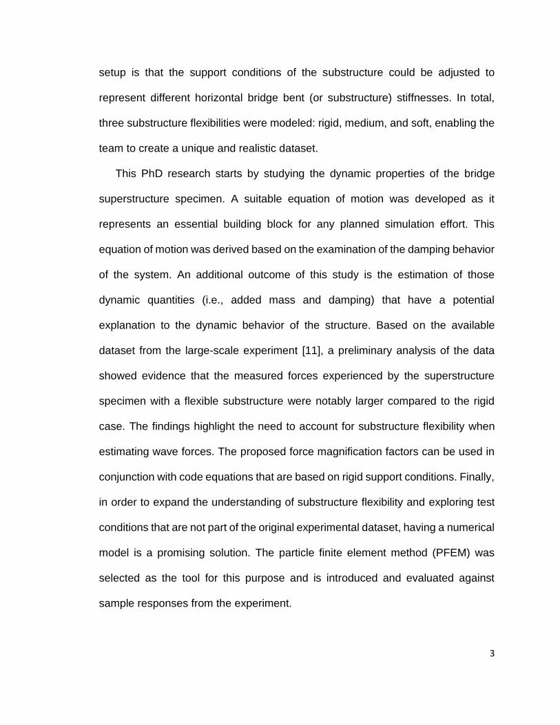
Figure 2.3. Example free vibration response for Phase 2b, dry trial: (a) time history and (b) frequency domain (Trial 2001: dry setting with soft spring).
The natural vibration frequencies, fn, for different springs at the different
water levels and all test trials are reported in Table 2.2. As can be observed, the
frequencies decreased with increasing water level, which is particularly obvious for
the fully submerged case of d* = +1. This can be explained by the concept of added
mass [25]–[27] whereby when a submerged body vibrates, it accelerates the
surrounding fluid particles, that act as additional mass and damping compared to
a body vibrating in air. For bodies submerged in water, this effect reduces the
natural frequency of the vibrating body and increases the damping compared to
what it would be in air [25]. Chandrasekaran et al. [25] also showed that the virtual
mass “depends on the geometry and the size of the structure, dynamic properties
of the structure in air (including its flexibility), the level of submergence, and the
type of excitation to which it is subjected.” Additionally, they report that the stiffness
of the structure is not affected by the level of submergence.

19
Table 2.2. Natural vibration frequencies, fn for different test trials and phases obtained by DFT.
d* Phase 2a
(medium springs)
Phase 2b
(soft springs)
dry Trial # 3001 3002 3003 2001 2002 2003
fn (Hz) 2.159 2.151 2.151 1.068 1.068 1.068
-1 Trial # 3101 3102 3103 2101 2102 2103
fn (Hz) 2.151 2.151 2.151 1.068 1.068 1.076
0 Trial # 3301 3302 3303 2301 2302 2303
fn (Hz) 2.132 2.132 2.129 1.060 1.060 1.060
1 Trial # 3501 3502 3503 2501 2502 2503
fn (Hz) 1.926 1.915 1.911 0.885 0.885 0.885
Following the research presented in [28], logarithmic decrements were
computed to identify the types of damping present in the system for all free
vibration test trials in this study. Figure 2.4 (a) shows the theoretical logarithmic
decrement behaviors obtained by solving the EOM via Runge-Kutta method for
three types of damping: linear viscous (i.e., when the damping force is proportional
to velocity), nonlinear viscous (i.e., when the damping force is a quadratic function
of velocity), and Coulomb (or friction) damping. The abscissa is interpreted as
vibration amplitudes decreasing in time. For linear viscous damping, the
logarithmic decrement is independent of the amplitude; therefore, it is a constant
value during vibration. For the nonlinear viscous damping case, the logarithmic
decrement is a function of amplitude and thus decreases linearly. Lastly, for friction
damping, the behavior is also dependent on the amplitude of vibration; however, it
increases exponentially. The amplitude values used in the computation of the
logarithmic decrements for Figure 2.4 were illustrated in Figure 2.3. The
logarithmic decrements measured for the free vibration response for all trials are
20
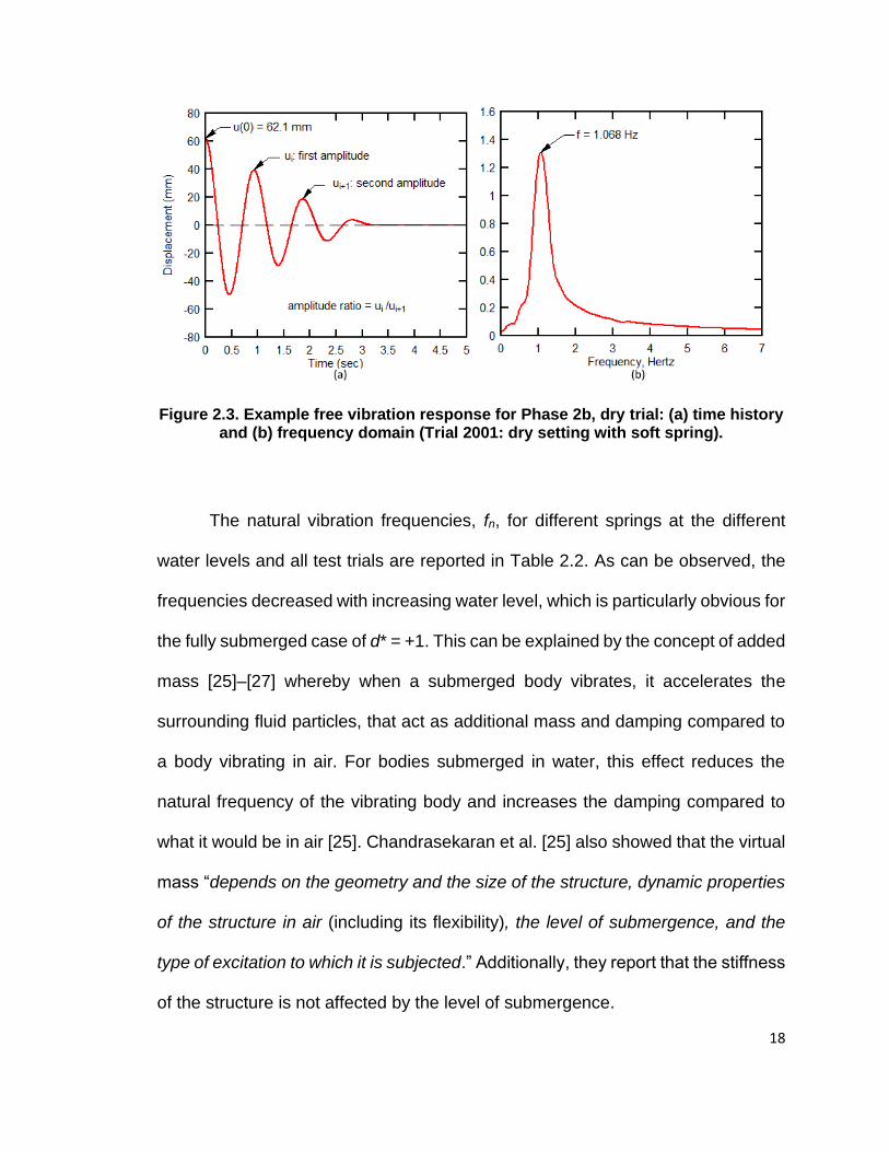
shown in Figure 2.4b. and are compared with the expected behaviors (theoretical
behavior) of the three damping models [28] (shown previously in Figure 2.4a).
Comparing Figure 2.4(a) and (b), one can observe that for the medium
spring setup (Phase 2a) the damping behavior follows that of a viscous damping
system at the beginning of the response; however, at the end of the response, the
behavior changes and resembles a friction damped system. For the soft spring
setup (Phase 2b), possibly because of the limited number of vibration cycles, the
behavior is not as clear for the submerged cases; however, for the dry trial it shows
a trend approximately following a friction damped system. The conclusion of these
results is that a combination of both viscous and friction damping exist for the
model and thus both need to be included in the EOM when creating a numerical
model of this bridge superstructure.
Figure 2.4. Comparison of logarithmic decrements for (a) theoretical values for three different types of damping following [26] and (b) free vibration tests from large-scale bridge superstructure model. The terminology in legend detailed in
Table 1.

21
2.5 Analysis
After studying the damping characteristics exhibited by the bridge model,
this section presents the relevant equation of motion (EOM), which is the first step
for analysis. Subsequently, the optimization scheme used to estimate the dynamic
parameters for the system is presented.
2.5.1 Numerical Model
The classic fourth-order Runge-Kutta (RK) numerical method [29] was
implemented in this study to solve the SDF equation of motion (EOM) for free
vibration of the large-scale experiment presented in [2]. Appendix A provides the
details of the implemented method along with a test for code verification. Based
on the findings presented in Section 4, the free vibration EOM implemented in this
study considers two types of damping forces simultaneously, viscous and friction
damping, as follows:
𝑚 ∙ �̈� + c ∙ �̇� + 𝐹 ∙ 𝑠𝑖𝑔𝑛(�̇�) + 𝑘 ∙ 𝑥 = 0 2.1
where m, c, and k represent mass, viscous damping coefficient, and stiffness
constant of the SDF system, F is the friction force, and �̈�, �̇�, and x are acceleration,
velocity, and displacement of the mass, respectively. Analytical solutions for the
steady-state response of a similar system excited with a harmonic force and
assuming a small friction force with no standstill regions were first presented by
Den Hartog [30] using a closed-form non-continuous solution. In other words, two
solutions based on the velocity sign, i.e. when �̇� > 0 and �̇� < 0, were used. Den

22
Hartog presented the solutions for several damping ratios as a function of the
amplification factor vs. frequency ratio with a discussion of the regions when
motion would or would not stop. Perls and Sherrard [31] extended Den Hartog’s
work for a wider range of damping ratios. Cheng and Zu [32] presented a different
analytical solution for the steady-state response of a system with combined
viscous and friction damping mechanisms subjected to two excitation forces with
different frequencies. Like Den Hartog, Cheng and Zu presented a discontinuous
solution due to discontinuities in the friction force function. Moreover, they
discussed two cases of motion behavior: when the motion is assumed not to have
a stopping region and when the motion experiences one stop. Feeny and Liang
[33] presented a methodology to quantify the damping coefficients for a system
with combined viscous and friction damping, assuming linearity of the system. This
led them to assume a linearly decreasing behavior for the successive extremes of
the displacement response, known as the displacement decrement identification
method. However, as was observed earlier in the logarithmic decrement analysis,
the decrement was not linear due to the nonlinearity of the system. Liang [34]
extended the previous work to identify the damping parameters from the
acceleration response, which they refer to as the acceleration decrement
identification method. Both methods are based on the discontinuous form of the
friction force function. Stanway and Mottershead [35] presented a numerical
comparison between three least-squares techniques to identify the damping
coefficient for a defined system using a continuous friction force function, by
assuming a constant friction force with a magnitude that is altered based on the

23
sign of velocity. This representation was modeled by introducing the term 𝐹 ∙
𝑠𝑖𝑔𝑛(�̇�). Finally, Mostaghel and Davis [36] suggested additional continuous
functions to represent the friction force-sliding velocity function. In this study, the
authors used the term 𝐹 ∙ 𝑠𝑖𝑔𝑛(�̇�) to represent the Coulomb friction damping force,
as previously described in [35], since, based on [36], it showed an instantaneous
phase change rather than any of the other presented functions. In addition, stop
motion behavior was not observed in the experimental results.
2.5.2 Parameter Estimation
Since the main objective of this study was to characterize the dynamic
properties associated with the effects of water submersion on the free vibration
response of the laboratory model, the unknown and most important parameters to
be estimated are: (a) viscous damping coefficient and (b) friction force. System
mass and stiffness could be directly computed from the experimental data [2].
Estimating (a) and (b) represents a classic inverse problem [37] where the
unknown input and known output parameters are the initial displacement as well
as level of submersion and the displacement response, respectively. The unknown
input parameters were obtained by varying them in the numerical model and
maximizing the correlation coefficient between the two responses. Using MATLAB
2017b [38], two methods were implemented for this optimization process. The first
one is referred to as “manual looping” where suitable ranges and increments for
each model parameter (e.g. damping ratio or friction force) were determined based
on the experimental results. By looping over these values, the best set of

24
parameters was found by maximizing the correlation coefficient between
experimental and numerically predicted vibration responses. The second method
is referred to as “global search” and utilizes a MATLAB built-in function called
GlobalSearch, which is a solver for optimization problems, e.g. to find a single
global minimum based on a user-defined objective function. The total absolute
error criteria was used to find the best-fit parameters. GlobalSearch operates a
local solver, fnimcon, which is designed to find solutions near the starting point
using a gradient-based method. Since the solution from this approach can be
influenced by the starting point itself, a heuristic approach was implemented
whereby multiple random starting points are employed to avoid the final solutions
being associated with a local minima.
Both methods were validated by first simulating a number of vibration
responses using a range of input parameters with the numerical approach
described in Section 5.1. The two optimization schemes were then used on these
simulated responses to estimate the input parameters. Globalsearch was able to
match the assumed input parameters with a maximum error of 1.9% where manual
looping led to larger errors (up to 11%) due to the finite increments required by the
method. Detailed results of this validation are provided in Appendix B.
Three levels of optimizations were initially evaluated using the two methods
with an increasing number of parameters to be estimated:
1. First level: damping ratio, 𝜻 and friction force, F (two variables)
2. Second level: mass, m damping ratio, 𝜻, and friction force, F (three
variables)

25
3. Third level: stiffness, k, mass, m, damping ratio, 𝜻, and friction force, F (four
variables)
While the second and third level optimizations usually produced results, the
objective functions for these two cases was likely relatively flat, leading to
unreasonable results for some of the trials. Thus, the optimization was ultimately
only performed for the first level, i.e. estimating damping ratio, 𝜁 and friction force,
F. For the manual looping method, the range of values for the viscous damping
ratio was set at 0 to 20% with 0.5% increments. For the friction force, the range
was set at 0 to 500 N using 10 N increments. The global search method uses a
scatter-search mechanism using the same ranges but without predefined
increments.
The spring stiffness, k, was computed for each trial as the slope from a
linear least squares regression on the force vs. displacement response taken when
the specimen was pulled to the initial displacement prior to release. Force and
displacement were measured with the horizontal load cell (LC) and the
displacement sensor labeled in Figure 2.1. An example force vs. displacement
response for Trial 2303 is shown in Figure 2.5 along with the mean prediction line
from the linear regression.

26
Figure 2.5. Example force - displacement response of model with mean prediction line from linear regression (Trial 2303, 3rd water level with soft springs).
Using k, and assuming that damping in the range considered does not
change the natural frequency, along with the computed natural vibration frequency,
fn (obtained from Table 2.2), the total vibrating mass, m could be estimated using
the following equation:
𝑚 = 𝑘 (2 ∙ 𝜋 ∙ 𝑓𝑛)2⁄ 2.2
The natural vibration frequencies of the dry trials were considered reference
values. Subsequent trials had higher water levels that produced added mass on
the system. Added mass, md, is defined as the difference between the total
vibrating mass computed from Eq. 3 and the reference mass, m computed in the
dry trials. Section 2.6 contains a detailed discussion of the added mass concept
and its use.

27
The results from the global search method were chosen for further use in
the study because they were more consistent and not bound to the values defined
by the fixed increments used in the manual looping search method. The estimated
parameters for all trials and both phases (medium and soft springs) determined
from the global search method are shown in Table 2.3. Mean, standard deviation,
and coefficient of variation (CV) for both stiffness and initial (dry) mass are also
reported here.
Table 2.3. Parameter estimates for all test trials obtained from the global search method.
Phase 2a
(medium springs)
Phase 2b
(soft springs)
Trial # k
(kN/m)
m
(kg)
md
(kg) 𝜻
F
(N) R2
k
(kN/m)
m
(kg)
md
(kg) 𝜻
F
(N) R2
Dry 449.2 2,458 -17 0.043 238 0.988 109.6 2,433 0 0.048 274 0.995
Dry 447.3 2,448 0 0.046 161 0.995 109.4 2,429 0 0.048 250 0.996
Dry 450.4 2,465 0 0.039 168 0.994 109.5 2,431 0 0.043 311 0.993
-1 444.1 2,430 0 0.040 174 0.991 109.6 2,433 0 0.059 254 0.995
-1 445.0 2,435 0 0.046 134 0.995 109.5 2,431 0 0.047 375 0.994
-1 447.7 2,450 0 0.037 162 0.995 109.9* 2,406 0 0.110 170 0.993
0 445.2 2,436 44 0.051 107 0.990 109.7 2,436 35 0.055 248 0.991
0 446.7 2,444 44 0.042 126 0.991 109.5 2,431 35 0.073 226 0.996
0 448.0 2,452 53 0.044 113 0.994 109.6 2,433 35 0.073 228 0.994
1 444.6 2,433 602 0.101 58 0.995 109.6 2,433 1111 0.106 311 0.993
1 444.1 2,430 637 0.097 58 0.996 109.7 2,436 1112 0.117 271 0.995
1 442.9 2,424 648 0.092 75 0.995 109.7 2,436 1112 0.089 388 0.993
Mean 446.3 2,442 109.6 2,433
STD 2.2 12.1 0.1 2.3
CV 0.49% 0.50% 0.09% 0.10%
*This result was considered an outlier and thus excluded from the analysis.
The values in Table 2.3 show an increasing trend for added mass and
hydroviscous damping with increasing water level, i.e. with greater submersion.
This corresponds to the findings of [25] that as the fundamental vibration period

28
increases the added mass should decrease. One additional note is that the values
presented as hydroviscous damping are not net values, rather they contain the
initial structural viscous damping component. In other words, the inherent viscous
damping of the structure in air is included in the values presented in Table 3 as
hydroviscous damping.

29
Figure 2.6. Box-and-whisker plot for the estimated parameters as a function of water level with median based estimation. Also shown are numerical values for
the means.
Figure 2.6 shows box-and-whisker plots for the estimated values of added
mass, hydroviscous damping, and the friction force (values taken from Table 2.3).
The friction force does not exhibit a specific trend for the soft springs setup (Phase

30
2b), although the range of these values fall within the observed sliding friction
values as found previously [23]. On the other hand, for the medium springs setup
(Phase 2a), the friction force decreases with increasing water level, which would
be expected. Moreover, the Phase 2b setup shows larger friction forces compared
to those of the Phase 2a setup. As was observed in the logarithmic decrement
analysis, the medium springs setup showed a more viscously damped behavior
while the soft spring setup exhibited a more frictionally damped behavior. This may
explain why the friction force for the medium springs setup was smaller compared
to the values for the soft springs setup. To gain deeper insight into the combined
effects of these parameters, a parametric study was performed and is presented
in Appendix C.
Figure 2.1 provides a comparison between the experimental results and the
numerical solutions using the dynamic parameters found by the optimization
procedure. Also shown are the values for added mass, damping ratio, friction force,
and the coefficient of determination, R2 between the two curves for each of the
selected trials. As can be observed, the two curves are almost identical, visually
demonstrating the ability of the optimization scheme to accurately estimate the
dynamic parameters from the free vibration trials.
Through the additional observations made from a parametric study (refer to
Appendix C) it became evident that added mass and damping ratio are
substantially influenced when the model was fully submersed. It had been argued
in some studies that the added mass effect is more significant than the effect due
to damping [26]. However, this argument depends on how the level of significance

31
is defined. In this study, both parameters play important roles in the dynamic
response of the test specimen alongside with the effect of friction damping. For
these experiments, the damping ratio ranged on average between 4.2 to 9.7% for
the medium springs setup (Phase 2a) and 4.6 to 10.5% for the soft springs setup
(Phase 2b). Added mass reached a value of 648 kg (26.6% of the dry mass) for
the medium springs setup and 1,112 kg (45.6% of the dry mass) for the soft springs
setup. Recall that the total mass of the superstructure model under dry conditions
is approximately 2,440 kg. The dynamic characteristics, i.e. added mass and
hydroviscous damping, appeared to have a greater effect for the soft springs setup.
In other words, for flexible substructures the added mass and damping should be
expected to be larger than for stiffer substructures.

32
Figure 2.7. Comparison between experimental data and numerical model for Phase 2a (medium springs setup) and 2b (soft springs setup) for select trials and
water levels. Also listed are the numerical values of the estimated parameter values.

33
2.6 Quantification of Added Mass Parameters
In this section, the concept of added mass is discussed in further detail.
When defining added mass, md, and considering only the fully submerged case,
there are two parameters that can be computed. The first one is the added mass
factor, 𝛼, which is the ratio between added mass, md and actual (or dry) mass, m,
and can be computed as [25]:
𝛼 = (𝑓𝑎 𝑓𝑤⁄ )2 − 1 2.3
𝑚𝑑 = 𝑚 ∙ 𝛼 2.4
where 𝑓𝑎 and 𝑓𝑤 are the natural vibration frequency of the structure in air and water
(fully submerged). The second parameter is referred to as added mass coefficient,
𝐶𝑚, which is defined as follows [26]:
𝐶𝑚 = 𝑚𝑑 𝑚𝑟𝑒𝑓⁄ 2.5
where 𝑚𝑟𝑒𝑓 is a reference fluid (or displaced fluid) mass defined as the mass of a
cylinder of fluid with a diameter equal to the dimension perpendicular to the
direction of motion as illustrated in Figure 2.8. This reference mass can be
computed as follows:
𝑚𝑟𝑒𝑓 = [𝜌𝑤𝑎𝑡𝑒𝑟 ∗ 𝐿 ∗ 2𝜋 ∗ (
𝐷
2)
2
] 2.6
where 𝜌𝑤𝑎𝑡𝑒𝑟 = 1000 𝑘𝑔/𝑚3 (freshwater was used for this study), and L and D are
the total width and depth of the structure perpendicular to the flow motion.

34
Figure 2.8. Parameters for the computation of the reference mass, mref.
For the case of partial submersion, the method of calculating the added
mass parameters differs as discussed in [25]. Also, because of the limitation in the
available data, the computation for the partially submerged cases is not addressed
here. Moreover, the analyzed data represent only one type of geometry, i.e. a
concrete deck-girder bridge superstructure with six girders. Both the geometric
limitation as well as the lack of partial submersion trials are considered for a future
study. As observed earlier, the structural stiffness influenced the added mass
factor and coefficient values. Table 2.4 presents the calculated values for the
added mass factor and the added mass coefficient for both test spring setups.
Table 2.4. Added mass factors and added mass coefficients calculated for both setups in fully submerged condition, 2a (= medium springs) and 2b (= soft
springs)*.
Added mass factor
Added mass value, kg
% of added mass from actual mass
Added mass coefficient
Phase 2a 𝛼2𝑎 0.262 𝑚𝑑,2𝑎 639 26% 𝐶𝑚,2𝑎 3.01
Phase 2b 𝛼2𝑏 0.456 𝑚𝑑,2𝑏 1113 46% 𝐶𝑚,2𝑏 5.23
*mref = 212.4kg, mactual (dry) = 2440kg

35
From the results of Table 2.4, the added mass coefficient can be interpreted
as follows: the hydrodynamic force acting on the cylinder is approximately 3.0
times the mass of fluid displaced times the acceleration of the flow for the medium
springs case, and 5.2 times the mass of fluid displaced times the acceleration of
the flow for the soft springs case. Table 2.5 reports a sample of the added masses
presented in [26], [39] for two cross sectional shapes: circle and rectangular, and
along three directions of excitations: one vertical (heave) and two horizontal
(surge, and sway) motions. It can be observed, for example, that in the vertical
motion, as the ratio of the side perpendicular to the movement direction (dimension
“a” in Table 2.5) to the side parallel to it increases, the added mass (hydrodynamic
mass) per unit length decreases. Comparing the two motion cases, added mass
seems to have the same magnitude. For the bridge specimen tested in this study,
the ratio was 0.144, therefore, the added mass coefficient is expected to be
between 1.98 and 2.23. The results from the present study show substantially
higher added mass compared to the reference values: 3.01 (1.35 times higher than
2.23 reference) for the medium springs setup and 5.23 (2.35 times higher than
2.23 reference) for the soft springs setup. Since the bridge deck specimen
contained chambers between the girders, which play as additional spaces for
water to fill in, that will contribute to increasing the observed added mass compared
to that for a solid structure. The large difference between the medium springs and
soft springs setups demonstrates how the substructure stiffness can strongly
influence the added mass.

36
Table 2.5. Hydrodynamic mass per unit length for circular and rectangular sections.
Section through body Translational direction
Hydrodynamic mass per unit length
Horizontal*,1
(surge) (sway)
𝑚𝑎𝑑𝑑𝑠𝑢𝑟𝑔𝑒 = 1 ∙ 𝜋 ∙ 𝜌 ∙ 𝑑2
𝑚𝑎𝑑𝑑𝑠𝑤𝑎𝑦 = 1 ∙ 𝜋 ∙ 𝜌 ∙ 𝑑2
Vertical2 (heave)
𝑚𝑎𝑑𝑑 = 1 ∙ 𝜋 ∙ 𝜌 ∙ 𝑎2
Horizontal1
(surge) (sway)
𝑚𝑎𝑑𝑑𝑠𝑢𝑟𝑔𝑒 = 1.51 ∙ 𝜋 ∙ 𝜌 ∙ 𝑎2
𝑚𝑎𝑑𝑑𝑠𝑤𝑎𝑦 = 1.51 ∙ 𝜋 ∙ 𝜌 ∙ 𝑎2
𝑎 𝑏⁄ = ∞ 𝑎 𝑏⁄ = 10
𝑎 𝑏⁄ = 5 𝑎 𝑏⁄ = 1
𝑎 𝑏⁄ = 1/5 𝑎 𝑏⁄ = 1/10
Vertical2 (heave)
𝑚𝑎𝑑𝑑 = 1 ∙ 𝜋 ∙ 𝜌 ∙ 𝑎2
𝑚𝑎𝑑𝑑 = 1.14 ∙ 𝜋 ∙ 𝜌 ∙ 𝑎2
𝑚𝑎𝑑𝑑 = 1.21 ∙ 𝜋 ∙ 𝜌 ∙ 𝑎2
𝑚𝑎𝑑𝑑 = 1.51 ∙ 𝜋 ∙ 𝜌 ∙ 𝑎2
𝑚𝑎𝑑𝑑 = 1.98 ∙ 𝜋 ∙ 𝜌 ∙ 𝑎2
𝑚𝑎𝑑𝑑 = 2.23 ∙ 𝜋 ∙ 𝜌 ∙ 𝑎2
* 𝑚𝑎𝑑𝑑 represent the added mass, 1: Ref. [37], 2: Ref. [24].
2.7 Summary and Conclusions
In this study, the dynamic response of a highway bridge superstructure
model was investigated using free vibration tests under varying degrees of
submersion to characterize the salient dynamic properties required for numerical
modeling of structural responses for fluid loading. In addition to varying water
levels, the substructure flexibility was also varied by inserting two sets of springs
with different stiffnesses into the experimental test setup. Friction force was
integrated into the equation of motion (EOM) to accurately capture the behavior of
the model. The dynamic response of the bridge model was significantly affected

37
by the level of submersion and substructure stiffness, resulting in different values
for damping and added mass. Consequently, these values (for damping and added
mass) affect the forces experienced on the structure and transmitted to
connections during highly-transient wave loading.
Numerical responses were generated by solving the EOM for a single
degree of freedom (SDF) mass-spring-damper system with combined viscous and
Coulomb friction damping via the classical 4th order Runge-Kutta numerical
method. An optimization scheme was used to estimate the dynamic properties of
the system, such as damping coefficient and friction force, by maximizing the
correlation coefficient between the observed and numerically simulated vibration
responses for each test trial. Based on the estimated parameters, the following
observations were made:
1. The natural vibration frequency of the bridge superstructure model
decreases with increasing water level (or submersion). In other words, the
added mass increases with increasing water level and for softer
substructure stiffness. This demonstrates that dynamic fluid-structure
responses are influenced by substructure stiffness.
2. Damping increases with increasing water level.
3. Dynamic fluid-structure responses are influenced by substructure stiffness.
Both added mass and damping coefficients were affected by the stiffness
of the substructure. Added mass and damping increased for the reduced
stiffness substructure.

38
4. The friction force, for the soft springs setup, stayed within the sliding friction
limits discussed in [2]. However, for the medium springs setup, the friction
force values were less than the sliding value limit and tended to decrease
as the water level increased.
The substructure flexibility was observed to influence the free-vibration dynamic
response of the model bridge when submersed in water. A properly developed
EOM is required to capture the bridge model response and it must include the
salient dynamic properties. Added mass and damping are important factors for
interpretation and understanding of fluid-structure response and can be used as
explanatory parameters in subsequent regression analyses.
2.8 References
[1] I. N. Robertson, H. R. Riggs, S. C. Yim, and Y. L. Young, “Lessons from Hurricane Katrina Storm Surge on Bridges and Buildings,” J. Waterw. Port Coast. Ocean Eng., vol. 133, no. 6, pp. 463–483, Nov. 2007, doi: 10.1061/(ASCE)0733-950X(2007)133:6(463).
[2] C. Bradner, T. Schumacher, D. Cox, and C. Higgins, “Experimental setup for a large-scale bridge superstructure model subjected to waves,” J. Waterw. Port Coast. Ocean Eng., vol. 137, no. 1, pp. 3–11, 2010.
[3] G. Cuomo, M. Tirindelli, and W. Allsop, “Wave-in-deck loads on exposed jetties,” Coast. Eng., vol. 54, no. 9, pp. 657–679, 2007.
[4] S. Douglass, Q. Chen, and J. Olsen, “Wave Forces on Bridge Decks Draft Report,” Coast. Transp. Eng. Res. Educ. Cent. Univ. South Ala., 2006.
[5] M. Hayatdavoodi, B. Seiffert, and R. C. Ertekin, “Experiments and computations of solitary-wave forces on a coastal-bridge deck. Part II: Deck with girders,” Coast. Eng., vol. 88, pp. 210–228, 2014.
[6] R. L. McPherson, “Hurricane induced wave and surge forces on bridge decks,” PhD Thesis, Texas A & M University, 2010.
[7] B. Seiffert, M. Hayatdavoodi, and R. C. Ertekin, “Experiments and computations of solitary-wave forces on a coastal-bridge deck. Part I: Flat plate,” Coast. Eng., vol. 88, pp. 194–209, 2014.
[8] D. Istrati, “Large-Scale Experiments of Tsunami Inundation of Bridges Including Fluid-Structure-Interaction,” PhD Thesis, 2017.

39
[9] P. Kaplan, J. J. Murray, and W. C. Yu, “Theoretical analysis of wave impact forces on platform deck structures,” American Society of Mechanical Engineers, New York, NY (United States), 1995.
[10] P. Kaplan, “Wave impact forces on offshore structures: re-examination and new interpretations,” in Offshore Technology Conference, 1992.
[11] J. Marin and D. M. Sheppard, “Storm surge and wave loading on bridge superstructures,” in Structures Congress 2009: Don’t Mess with Structural Engineers: Expanding Our Role, 2009, pp. 1–10.
[12] Q. Chen, L. Wang, and H. Zhao, “Hydrodynamic investigation of coastal bridge collapse during Hurricane Katrina,” J. Hydraul. Eng., vol. 135, no. 3, pp. 175–186, 2009.
[13] D. James, J. Cleary, and S. Douglass, “Estimating Wave Loads on Bridge Decks,” in Structures Congress 2015, 2015, pp. 183–193.
[14] G. Xu and C. S. Cai, “Wave forces on Biloxi Bay Bridge decks with inclinations under solitary waves,” J. Perform. Constr. Facil., vol. 29, no. 6, p. 04014150, 2014.
[15] A. Guo, Q. Fang, X. Bai, and H. Li, “Hydrodynamic experiment of the wave force acting on the superstructures of coastal bridges,” J. Bridge Eng., vol. 20, no. 12, p. 04015012, 2015.
[16] J. Jin and B. Meng, “Computation of wave loads on the superstructures of coastal highway bridges,” Ocean Eng., vol. 38, no. 17–18, pp. 2185–2200, 2011.
[17] J. Marin and D. M. Sheppard, “Storm surge and wave loading on bridge superstructures,” in Structures Congress 2009: Don’t Mess with Structural Engineers: Expanding Our Role, 2009, pp. 1–10.
[18] “Development of the AASHTO guide specifications for bridges vulnerable to coastal storms | Request PDF,” ResearchGate. https://www.researchgate.net/publication/299678527_Development_of_the_AASHTO_guide_specifications_for_bridges_vulnerable_to_coastal_storms (accessed Nov. 09, 2018).
[19] X. Chen, J. Zhan, Q. Chen, and D. Cox, “Numerical Modeling of Wave Forces on Movable Bridge Decks,” J. Bridge Eng., vol. 21, no. 9, p. 04016055, Sep. 2016, doi: 10.1061/(ASCE)BE.1943-5592.0000922.
[20] G. Xu and C. S. Cai, “Numerical simulations of lateral restraining stiffness effect on bridge deck–wave interaction under solitary waves,” Eng. Struct., vol. 101, pp. 337–351, 2015.
[21] G. Xu and C. S. Cai, “Numerical investigation of the lateral restraining stiffness effect on the bridge deck-wave interaction under Stokes waves,” Eng. Struct., vol. 130, pp. 112–123, 2017.
[22] T. Schumacher, C. Higgins, C. Bradner, D. Cox, and S. C. Yim, “Large-Scale Wave Flume Experiments on Highway Bridge Superstructures Exposed to Hurricane Wave Forces,” presented at the Sixth National Seismic Conference on Bridges and HighwaysMultidisciplinary Center for Earthquake Engineering ResearchSouth Carolina Department of TransportationFederal Highway AdministrationTransportation Research Board, 2008, Accessed: Mar. 09, 2020. [Online]. Available: https://trid.trb.org/view/1120856.
[23] C. Bradner, Large-scale laboratory observations of wave forces on a highway bridge superstructure. Oregon State University, 2008.
[24] C. Bradner, T. Schumacher, D. Cox, and C. Higgins, “Large–Scale Laboratory Observations of Wave Forces on a Highway Bridge Superstructure,” 2011.
[25] A. R. Chandrasekaran, S. S. Siani, and M. M. Malhorta, “Virtual mass of submerged structures,” J. Hydraul. Div., vol. 98, no. 8923 Paper, 1972.

40
[26] R. G. Dong, “Effective mass and damping of submerged structures,” California Univ., Livermore (USA). Lawrence Livermore Lab., 1978.
[27] R. J. Fritz, “The effect of liquids on the dynamic motions of immersed solids,” J. Eng. Ind., vol. 94, no. 1, pp. 167–173, 1972.
[28] E. Nezirić, S. Isić, V. Doleček, and A. Voloder, “An Analysis of Damping type Influence to Vibration of Elastic Systems,” 2010.
[29] J. F. Epperson, An Introduction to Numerical Methods and Analysis. John Wiley & Sons, 2013.
[30] J. D. Hartog, “LXXIII. Forced vibrations with combined viscous and coulomb damping,” Lond. Edinb. Dublin Philos. Mag. J. Sci., vol. 9, no. 59, pp. 801–817, 1930.
[31] T. A. Perls and E. S. Sherrard, “Frequency response of second order systems with combined Coulomb and viscous damping,” J. Res. Natl. Bur. Stand., vol. 57, no. 1, p. 45, 1956.
[32] G. Cheng and J. W. Zu, “Two-frequency oscillation with combined Coulomb and viscous frictions,” J. Vib. Acoust., vol. 124, no. 4, pp. 537–544, 2002.
[33] B. F. Feeny and J. W. Liang, “A decrement method for the simultaneous estimation of Coulomb and viscous friction,” J. Sound Vib., vol. 195, no. 1, pp. 149–154, 1996.
[34] J.-W. Liang, “Identifying Coulomb and viscous damping from free-vibration acceleration decrements,” J. Sound Vib., vol. 282, no. 3–5, pp. 1208–1220, 2005.
[35] R. Stanway and J. E. Mottershead, “Identification of combined viscous and Coulomb friction-a numerical comparison of least-squares algorithms,” Trans. Inst. Meas. Control, vol. 8, no. 1, pp. 9–16, 1986.
[36] N. Mostaghel and T. Davis, “Representations of Coulomb friction for dynamic analysis,” Earthq. Eng. Struct. Dyn., vol. 26, no. 5, pp. 541–548, 1997.
[37] J. C. Santamarina and D. Fratta, Discrete signals and inverse problems: an introduction for engineers and scientists. John Wiley & Sons, 2005.
[38] “How GlobalSearch and MultiStart Work - MATLAB & Simulink.” https://www.mathworks.com/help/gads/how-globalsearch-and-multistart-work.html (accessed May 19, 2018).
[39] Techet, “2.016 Hydrodynamics _ Added Mass,” . [40] P. J. Roache, Verification and validation in computational science and engineering,
vol. 895. Hermosa Albuquerque, NM, 1998. [41] B. A. Erickson and E. M. Dunham, “An efficient numerical method for earthquake
cycles in heterogeneous media: Alternating subbasin and surface-rupturing events on faults crossing a sedimentary basin,” J. Geophys. Res. Solid Earth, vol. 119, no. 4, pp. 3290–3316, 2014.

41
Chapter 3
Manuscript 2: Effect of Substructure Flexibility on Wave-induced Forces on
Bridge Superstructures
This manuscript is co-authored by Thomas Schumacher (adviser), Christopher
Higgins, and Avinash Unnikrishnan. This manuscript is currently being prepared
for submission to a journal.
3.1 Introduction and Background
A common failure mode of coastal bridges after the hurricane impacts in
2004 (Katrina) and 2005 (Ivan) was attributed to strength-deficient connections
between superstructure and substructure. Once these connections had failed,
wave loads were in many cases large enough to move superstructures off their
substructures into the water [1], as can be observed in Figure 3.1.
Figure 3.1. Photo of superstructures of the US 90 Biloxi Bay Bridge that have been removed from their substructures by wave loads during Hurricane Katrina. Source
[2].

42
Prior to the hurricane events in the early 2000s, it was thought that the
superstructure’s self-weight, along with shear-keys, would be sufficient to resist
any hurricane-induced wave forces. The reason for the observed system failure is
that the storm surge was much higher than anticipated, which lead to vertical, i.e.
uplift, forces that were, in combination with the large horizontal forces, exceeding
the capacity of the commonly used girder anchorage systems [3]. In many cases,
no major damage was observed on the superstructures or to the substructures.
Studying and providing stronger connections, i.e. anchorages, between girders
and bent-caps has thus been proposed. The caveat is that stronger connections
have the ability to transfer higher forces between superstructures and
substructures. Therefore, it becomes necessary for the substructure to be able to
carry these higher forces. Assuming the presence of anchorages that can transfer
any forces, substructure flexibility is thus a factor that might significantly affect the
experienced wave forces on bridge superstructures. To address these questions,
Bradner et al. [4] tested a realistic 1:5-scale highway bridge model under various
wave conditions experimentally. The setup is unique in that the horizontal flexibility
of the substructure representing the bent columns, bent cap, and foundation, could
be adjusted by inserting springs of different stiffness. The reported experiments
were performed for three different substructure stiffnesses, including rigid (no
springs), medium, and soft. The stiffnesses of the springs were selected based on
2D frame analyses of realistic substructure configurations [5], [6]. While some
preliminary results have been reported [2], [4]–[6], no systematic analysis has been
performed to date. Schumacher et al. in [2] qualitatively showed that the wave-

43
induced forces for a flexible setup are larger compared to a rigid setup. In [4]–[6],
they showed that a second-order polynomial relationship between wave height and
wave forces could be defined for both regular and random waves. Also, they
addressed the effect of water level. They showed that, for the first three levels,
forces were increased as water level increased. However, as the structure started
to submerge until it got fully submerged, forces start to level off or even decrease.
In this study, these observations are reinforced by a statistical test emphasizing
the effect of substructure flexibility, besides the derivation of factors that account
for this effect. Additionally, wave forces on coastal structures, particularly bridges,
attracted the attention of many other researchers, who studied them
experimentally [6]–[12] or numerically [13]–[20]. Through these efforts, many
concepts and theories regarding wave-structure interaction dynamics have been
established and equations for estimating wave forces developed. Additionally, an
AASHTO guide has been developed to calculate horizontal and vertical forces, as
well as overturning moment for highway bridge superstructures having a variety of
girder types [21]. Most of the aforementioned research has focused on bridge
systems where the substructure is assumed to be rigid horizontally. Some recently
conducted numerical studies have studied the effects of horizontal fixity issue and
submersion depth on the experienced forces [17], [18]. Both of these studies found
that the induced wave forces increase with increasing flexibility of the structure.
Most coastal engineers use normalized features in their analyses as a way
to generalize the results [22]. One advantage is that these non-dimensional

44
analyses help in reducing the scattering in the estimated values and provides
physics-based models that are less sensitive to superior correlations [22].
For example, air trapped under a bridge deck between girders has been
studied as a factor affecting the wave forces acting on an elevated coastal bridge
deck [23]. The procedure for analyzing the data was to filter the collected signals
using the wavelet transform of the recorded signals, and distinguish the forces’
time history to have two regions: short time wave application (slamming force) and
long-time wave application (quasi-static force). In their analysis, the researchers
normalized the measured pressure by the static-equivalent pressure (𝜌𝑔𝐻), where
𝜌 is water density, 𝑔 is the gravitational acceleration, and 𝐻 wave height, and
plotted them against the hydrostatic head (𝜂−𝑐
ℎ), where 𝜂 is the wave elevation, 𝑐 is
the clearance between the still water level and the bottom of the structure, and ℎ
is the water depth. Hydrostatic head could be interpreted as the relative wetted
area. Three distinct regions were observed in the analyzed data and they were
attributed to the structural inundation level. These regions are defined as follows:
1. Hydrostatic head < 0: rapid increase in loading
2. 0 < Hydrostatic head < 0.4: slow increase in loading.
3. 0.4 < Hydrostatic head < 0.65: rapid increase in loading.
Openings introduced in the deck to relief trapped air showed a decrease on
the measured forces.
AASHTO [21], on the other hand, counted for this factor (air entrapment)
which was defined by calculating the trapped air factor (TAF). TAF in turn was a

45
function of several parameters: submersion depth, bridge width, and girders
depths per their specifications. This factor defines a wide rank (0 -100%)
depending on the designer decision.
[7] found that vertical force was highly affected by air entrapment, and by
introducing openings in the deck, the vertical forces decreased.
Using potential flow theory, Guo et al. [19] studied the behavior of forces
normalized by (𝜌𝑔ℎ𝐴) vs. wavenumber (k = 1/𝜆) as the independent variable, with
𝐴 being the area by which the wave interacts with the structure, and 𝜆 being
wavelength. Two equations where derived to estimate vertical and horizontal
forces. In their study they showed that the normalized vertical force experienced a
dramatic decrease by an increase of wave numbers ≤ 1.0, after this point (i.e. for
wave numbers > 1.0) the vertical force decreased slowly. For horizontal force, a
reversed behavior was observed. For wave number ≤ 1.0, the normalized
horizontal force increased dramatically as k increased. For 1.0 ≤ k < 1.5, the
normalized horizontal force slowly increased. For k > 1.5, the normalized horizontal
force exhibited a decreasing trend.
Using the last numerical model presented in [19], Fang et al. [20] studied
the effect of incident angle on wave forces on bridge superstructures. Similarly,
they employed normalized features in their analyses and showed that the
perpendicular direction produces the highest wave forces. Three additional
normalized parameters were studied besides the angle of action. The first one is
submersion depth normalized by water depth. The other parameter was the
relative thickness of the bridge, which was measured by dividing deck thickness

46
by the submersion depth. The third parameter was the number of girders. All three
parameters were shown to affect the horizontal force, whereas they had no effect
on the vertical force components.
Hayatdavoodi et. al. [24] studied the effect of solitary and cnoidal waves on a
submerged horizontal deck on the normalized horizontal force, vertical force, and
overturning moment (around the middle of the deck). Wave height, wave period,
deck submersion, and deck width were among the studied parameters after they
were normalized. Simplified empirical equations were developed based on the
numerical results. Their findings can be summarized as follows:
For solitary waves:
a. Vertical force, horizontal force, and overturning moment linearly increase
with increasing wave height.
b. Vertical force and overturning moment increase with increasing deck width.
The horizontal force reaches a constant value after the deck width reaches
a certain value.
c. The level of submersion has little effect (if none) on the forces, in general.
For cnoidal waves:
a. Forces change nonlinearly with wave height.
b. Vertical force and overturning moment decrease with increasing level of
submersion. The horizontal force remains constant after a certain level of
submersion is reached.
47
c. Vertical force and overturning moment increase nonlinearly with increasing
deck width, whereas the horizontal force oscillates.
Finally, Park et al. [25] normalized wave forces by the incident wave energy
along the shoreline and plotted them against normalized clearance by water depth,
which can be thought of as relative water depth. The normalized forces by the
incident wave energy is a measure of energy dissipation. Following in this study,
the normalized wave forces by the incident wave energy vs. the relative width will
be examined.
3.2 Motivation and Objectives
The effect of horizontal flexibility of the substructure representing bent
columns, bent cap, and foundation, have not been studied sufficiently. In fact, the
two studies found, i.e. [15], [17], actually contradict each other as to whether
flexible support conditions lead to increased or decreased wave-induced forces.
Additionally, current design guides are based on rigid substructure conditions,
which from a structural engineering perspective are not realistic [21]. The
motivation of the work presented in this article, which is based on the unique
dataset described in [4], was to study the effect of substructure flexibility and
develop force magnification factors that bridge engineers can use in conjunction
with prediction equations to estimate wave forces on bridge superstructures.

48
3.3 Experimental Setup
The analysis presented in this article is based on data produced from a
large-scale experimental research project conducted in the O.H. Hinsdale Wave
Research Laboratory at Oregon State University [4]. Details of the experimental
setup as well as testing protocols and some preliminary data can be found in [4],
[6]. Only a brief overview of the experiment is given subsequently. Figure 3.2
shows an elevation view of the realistic 1:5-scale highway bridge superstructure
model used in the experiments as well as some of the instrumentation. The three
different horizontal support conditions representing three different substructure
flexibilities are highlighted as well and include: Phase 1, 2a, and 2b. These
correspond to rigid, medium, and soft horizontal support conditions, respectively.
Numerical values are summarized in Table 3.1.
Table 3.1. Structural configurations and test phases investigated in [6] and used in this study.
Phase Horizontal support condition
Model spring stiffness
kN/m (lb/in)
Connection between model superstructure and bent cap
1 Rigid Very large
Fixed, bolted (assumed rigid) 2a Dynamic, medium
springs 458 (2614)
2b Dynamic, soft springs 107 (612)
3* Unconstrained N/A None (free, held by gravity and friction)
* Data from this test phase was not used in this study.

49
Figure 3.2. Elevation view of experimental test setup showing different horizontal support conditions, i.e. test phases (LC = load cell, SWL = still water level).
Dimensions: m (ft). (Courtesy of Dr. Schumacher).
Figure 3.3 illustrates a bridge superstructure under wave action and
provides commonly used terminology, which is also used herein.

50
Figure 3.3. Elevation view of bridge superstructure under wave action with commonly used terminology. (Courtesy of Dr. Schumacher).
In the experiment [6], five still water levels (SWL), corresponding to depths
ranging from h = 1.61 m to 2.17 m, were studied with increments of 0.14 m, which
is equal to one-half of the total depth of the bridge superstructure, hd. Let 𝑧𝑑
represent the elevation of the bridge specimen measured from the bottom of the
girders, which is equal to the water depth (h) plus the clearance (c). Subsequently,
normalized water levels are referred to and are calculated as follows:
𝑑∗ =
ℎ − 𝑧𝑑
ℎ𝑑 3.1
The range of normalized depths is thus -1.0 to 1.0 with increments of 0.5. In the
text we also refer to first to fifth water level, which correspond to d* = -1.0 to +1.0,
respectively.

51
Table 3.2. Studied still water levels (SWL).
Description Water depth, h
(m)
clearance, c
(m)
Normalized water
level d* (-)
First water level 1.61 +0.28 -1.0
Second water level 1.75 +0.14 -0.5
Third water level 1.89 0.00 0
Fourth water level 2.03 -0.14 0.5
Fifth water level 2.17 -0.28 1.0
Figure 3.4. Sample experimental measurements for d* = 0.0, T = 3.0 s, H = 0.625 m, Phase 1: Time histories of (a) Water level at WG 9, 4.21 m (13.8 ft) away from front
face of the bridge model, (b) total horizontal force, (c) total vertical force (WG = wave gage).
Figure 3.4 shows sample measurements for a select wave trial for Phase 1
(rigid setup). Note that the total horizontal force is the summation of the two
horizontal load cells measurements, whereas the total vertical force is the

52
summation of all four vertical load cells (two offshore and two onshore).
Researchers define wave force as having two components, horizontal and vertical,
that are used to identify the forces experienced by a structure. Each component
has two distinct regions; positive that increases until reaching the force maximum
positive value and negative that decreases until reaching the force maximum
negative value. The forces that are analyzed and processed are those that capture
the dynamic action of the bridge superstructure. In this article the net positive
forces were considered in the analysis. Figure 3.5 shows a close-up view of
sample time histories for total vertical force that show these two regions. The same
can be applied for total horizontal force. Different windows were selected for each
wave force time history (which corresponds to a single trial), over which the
average was computed, which represented one sample measurement in the data
set.

53
Figure 3.5. A close-up view for a sample time-history for a total vertical force due to two passing waves.
In Figure 3.6, the time histories for the fixed/rigid (Phase 1) and soft (Phase
2b) setups at the second water level (d* = -0.5) with a wave period, T = 2.5 s for
both vertical and horizontal forces are shown for comparison. As can be observed,
the behavior of the horizontal wave force differs significantly between the two
substructure flexibilities. For the flexible condition, besides the increase in wave
force, the horizontal force is smooth and dominated by the spring stiffness,

54
whereas for the vertical force response, not much difference in the behavior except
for a slight increase in the force magnitude can be observed.
Figure 3.6. A close-up view for a sample time-history for the effect of substructure fixity on the on the observed wave force at same wave condition.
Subsequently, the effect of substructure flexibility on the forces experienced
by the bridge superstructure model are analyzed and discussed through
presenting parameters that the authors believe to be important in understanding
and estimating wave forces. These parameters are organized in two categories:
unnormalized features (parameters), and normalized features (parameters), as
suggested in the literature.

55
3.4 Data Analysis
In this section, visualizations are done to the experimental data through
presenting two categories of the commonly used parameters through the literature
in defining wave forces. These categories are unnormalized and normalized
features. Levels of submersion, wave height, wave steepness, and wave celerity
are features presented under the unnormalized features. Normalized features
analyzed include normalized forces by the incident wave energy along with the
relative width.
The main point of this section is to show how substructure flexibility affects
the magnitude of the induced wave forces considering these different features, set
the stage for future work in building refined models that account for substructure
flexibility, and provide physical interpretations for the reason why structures with
flexible supports have larger forces.
3.4.1 Unnormalized feature analysis
Plotting data is an important key to depicting interesting features of possible
relationships between the defined variables. As seen earlier, many parameters
were believed to have an influence on the magnitude of the measured forces. In
Figure 3.7, box plots of horizontal and vertical wave forces are drawn vs.
normalized water level, d* for waves with wave height, H = 0.5 m, and wave period,
Tp = 2.5 s. It can be observed that both horizontal and vertical wave force
components increase with increasing water level, reaching their maxima (in this
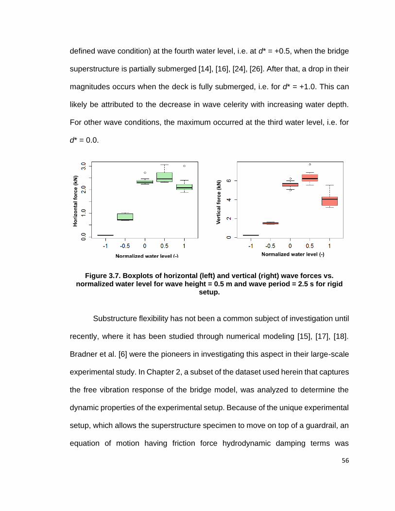
56
defined wave condition) at the fourth water level, i.e. at d* = +0.5, when the bridge
superstructure is partially submerged [14], [16], [24], [26]. After that, a drop in their
magnitudes occurs when the deck is fully submerged, i.e. for d* = +1.0. This can
likely be attributed to the decrease in wave celerity with increasing water depth.
For other wave conditions, the maximum occurred at the third water level, i.e. for
d* = 0.0.
Figure 3.7. Boxplots of horizontal (left) and vertical (right) wave forces vs. normalized water level for wave height = 0.5 m and wave period = 2.5 s for rigid
setup.
Substructure flexibility has not been a common subject of investigation until
recently, where it has been studied through numerical modeling [15], [17], [18].
Bradner et al. [6] were the pioneers in investigating this aspect in their large-scale
experimental study. In Chapter 2, a subset of the dataset used herein that captures
the free vibration response of the bridge model, was analyzed to determine the
dynamic properties of the experimental setup. Because of the unique experimental
setup, which allows the superstructure specimen to move on top of a guardrail, an
equation of motion having friction force hydrodynamic damping terms was

57
developed and its dynamic parameters quantified. This equation of motion is
essential to build any numerical model of this particular experimental setup [5].
Some researchers who implemented numerical modeling did not consider the
appropriate damping terms in their work [15], [17], [18]. As a result, inconsistencies
between their results and the experimental data of [5] can be observed. As
presented in [15], wave forces experienced a reduction in their magnitudes with
increasing support flexibility. Contradicting this finding, [17] showed that wave
forces were increasing with increasing support flexibility. To answer the question
whether increasing substructure flexibility leads to increasing or decreasing wave
forces, a series of plots are interpreted subsequently.
Figure 3.8 shows the behavior of wave forces vs. wave heights for different
substructure flexibilities, which are shown in different symbols and colors.
Normalized water depth, d* = +0.5 and wave period, Tp = 2.5 s. Both horizontal
and vertical wave forces with their mean values within a selective window of their
actual response are presented. Distinct features can be observed. The forces
experienced for the soft substructure flexibility are larger than those experienced
for the rigid case, as proposed in [2], [17], and the difference increases linearly
with increasing wave height, reaching a value of approximately 38% for a wave
height of 0.58 m. Therefore, increasing substructure flexibility make a structure
more susceptible to wave action, especially when the structure interferes with the
water body (i.e., for partially submerged cases), putting the bridge superstructure
in the maximum fluid flow field, and the surrounding water body starts to add
additional mass to the moving structure. This additional mass increases the

58
momentum induced in the structure, which leads to increased forces experienced
to be sustained by the structure. This also could be linked to the drag force. Drag
force plays a role in determining the wave forces, since it is related to the projected
area of interaction and wave celerity [27], [28].
Figure 3.8. Scatter plots of (a) horizontal and (b) vertical wave forces vs. wave height. Normalized water depth, d* = +0.5 and wave period, Tp = 2.5 s.
Appendix D shows the remaining cases of wave forces vs. wave heights for
wave periods 𝑇𝑃 = 2, 2.5, and 3.0 s and for all five water levels. From these figures,
it seems that the action of a wave will not be noticed until its height reaches a
certain level. A positive correlation between wave forces and wave height be
found, which is intuitive and has been confirmed by others [2], [4]–[6]. As water
level increase, the role of wave height is more significant up to the third water level
when it is starting to decline, as observed from the inclination of the line formed by
the data.

59
Another unnormalized feature that may affect wave forces is wave
steepness, which is calculated by dividing the wave height by the wavelength.
Figure 3.9 depicts the relation between wave forces and wave steepness. As wave
steepness increases (which an indication of wave energy increase) the induced
wave forces increase as well.
Figure 3.9. Scatter plots of (a) horizontal and (b) vertical wave forces vs. wave steepness. Normalized water depth, d* = +0.5 and wave period, Tp = 2.5 s.
Wave celerity (or velocity) is another factor thought to be one of the
important features shaping wave force magnitudes, since it is related to forces via
the drag term. Again, a positive correlation can be observed between wave celerity
and wave-induced forces, as visualized in Figure 3.10.
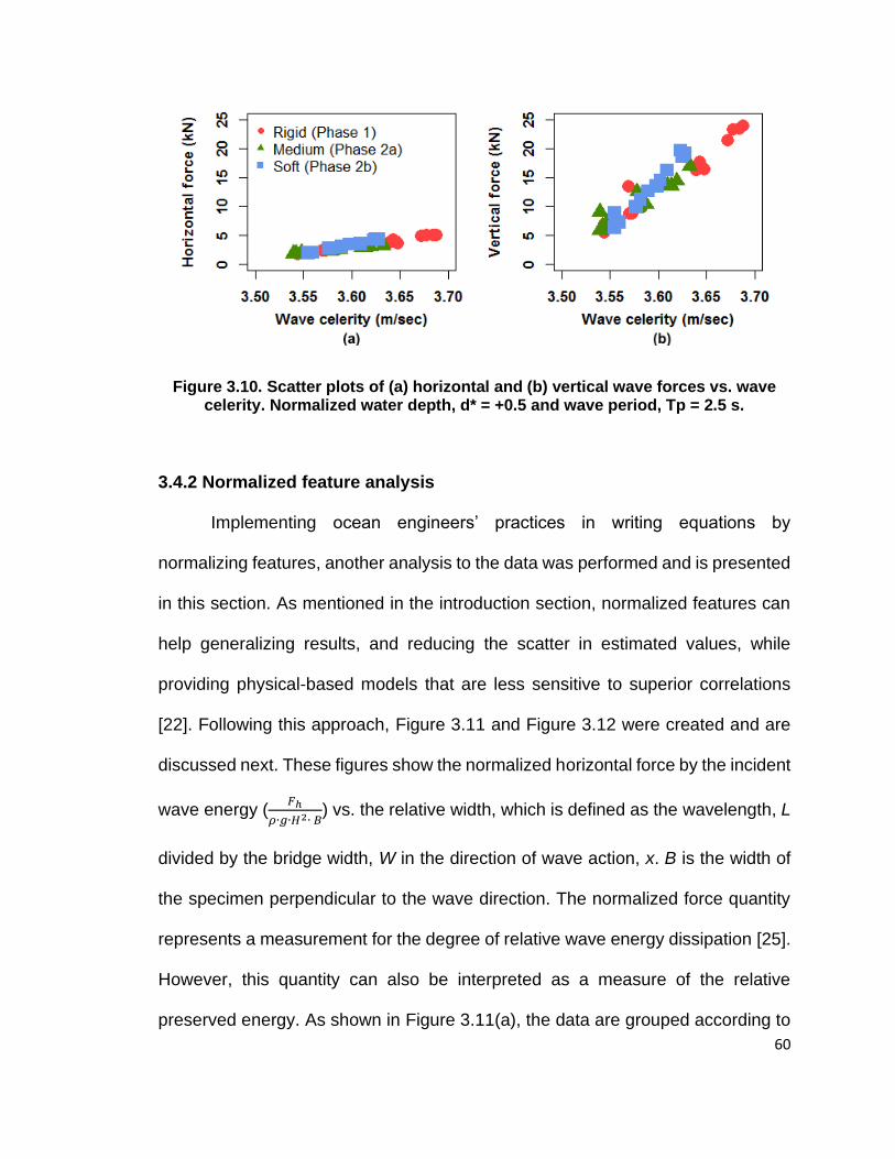
60
Figure 3.10. Scatter plots of (a) horizontal and (b) vertical wave forces vs. wave celerity. Normalized water depth, d* = +0.5 and wave period, Tp = 2.5 s.
3.4.2 Normalized feature analysis
Implementing ocean engineers’ practices in writing equations by
normalizing features, another analysis to the data was performed and is presented
in this section. As mentioned in the introduction section, normalized features can
help generalizing results, and reducing the scatter in estimated values, while
providing physical-based models that are less sensitive to superior correlations
[22]. Following this approach, Figure 3.11 and Figure 3.12 were created and are
discussed next. These figures show the normalized horizontal force by the incident
wave energy (𝐹ℎ
𝜌∙𝑔∙𝐻2∙ 𝐵) vs. the relative width, which is defined as the wavelength, L
divided by the bridge width, W in the direction of wave action, x. B is the width of
the specimen perpendicular to the wave direction. The normalized force quantity
represents a measurement for the degree of relative wave energy dissipation [25].
However, this quantity can also be interpreted as a measure of the relative
preserved energy. As shown in Figure 3.11(a), the data are grouped according to

61
wave periods, Tp with an interesting behavior of the normalized wave forces. This
behavior defines an inflection point between short and long wave periods. These
two regions were observed in [15] through a different comparison. In [15], they
showed that for short wave periods (𝑇𝑝 < 3.0) wave celerity plays a major role,
whereas for longer wave periods (𝑇𝑝 > 3.0), it plays a secondary role. This can be
explained by the limitations in wave steepness, which required no wave breaking
or flume overflow, therefore, wave celerity gets slower for the same wavelength as
wave height decreases, and that is why we see a reduction in the energy level. As
a result, for further analyses, normalized forces generated by waves with periods,
Tp = 2.5 s are examined, as shown in Figure 3.11(b).
Figure 3.11. Scatter plots of normalized horizontal wave force vs. relative width.
Figure 3.11 (b) visualizes the different substructure flexibility effects on the
measured forces. A more rigorous analysis is done to Figure 3.11(b) in Figure 3.12.
A clear distinction between the three flexibility configurations shows that a
superstructure with a flexible substructure has the least wave energy dissipation,
or the highest relative energy preservation from the wave application. Additionally,

62
waves with wave height, H = 0.375 m show the highest relative energy
preservation from wave action compared to other wave heights starting from the
third water level. In another words, when the wave height is almost a full projection
on the superstructure depth - i.e. complete wave interaction with the structure - the
relative preserved wave energy by the superstructure is the highest. However, at
initial water levels (the superstructure is above the still water level), as wave height
increases, the more wave energy is preserved. This means wave height plays a
significant role in adding more force to the structure when the superstructure is
elevated. This observation reinforces the conclusion made in the previous section.

63
Figure 3.12. The relative energy preservation at different water levels and wave
heights.
3.5 Substructure Flexibility Effect
Motivated by the strong evidence of the substructure flexibility influence on
the induced wave force magnitudes, this section quantifies the amount of
magnification. As suggested by [2], an anticipated quadratic relation could be
observed between wave forces and wave height. Therefore, a linear least-squares
first-order curve fit was used to describe the relation between the square root of
wave force and wave height. The curve was forced to pass through the origin,

64
ensuring that zero wave height corresponds to zero force. Additional data
processing prior to the regression process was needed for the first and second
water levels, since at these water levels certain minimum wave heights are
required to produce any wave forces. Therefore, a shift in the x-axis equal to the
clearance between the still water level and the bottom of the superstructure
girders, which reflect the height that the wave needs to reach before have some
interaction with specimen. In Figure 3.13 and Figure 3.14, the mean curve fit lines
along with 95% prediction limits for both horizontal and vertical forces and wave
height are shown. Finally, force magnification factors were calculated by dividing
the computed slopes for the two flexible setups by the slope of the rigid setup (the
reference case). Since three slopes, corresponding to mean, lower, and upper
95% prediction limits, were available for each case, force magnification factors
using combinations were computed.
Recall that the data used to generate these curve fits are represented by
the average value of 5 to 7 peaks in series for a selected window of loading cycles,
as shown in Figure 3.5. Three windows per one trial were defined and their average
were computed. The magnification factors for all five water levels and three wave
periods are included in Appendix E.

65
Figure 3.13. Illustration of force magnification factors for sample horizontal force with d* = 0.0 and Tp = 2.5 s: (a) Mean curve fit lines along with 95% prediction limits for the horizontal wave forces and (b) force magnification factors for
different substructure flexibilities, considering the rigid condition as the reference value. Error bars represent 95% prediction limits of the curve fits.
Figure 3.14. Illustration of force magnification factors for sample vertical force with d* = 0.0 and Tp = 2.5 s: (a) Mean curve fit lines along with 95% prediction
limits for the vertical wave forces and (b) force magnification factors for different substructure flexibilities, considering the rigid condition as the reference value.
Error bars represent 95% prediction limits of the curve fits.
To find if the slopes of the fitted regression lines for the flexible setups are
significantly different from the fitted regression lines for the rigid setup, tests of

66
restrictions were run for all different cases of water levels and wave periods. In
these tests, two models are generated. The full model (or: unrestricted model) is
one which assumes that the slope of the regression line fitted to the whole data is
affected by both data setups (rigid and flexible), which can be written as:
√𝐹𝑜𝑟𝑐𝑒 = 𝑚𝑟𝑖𝑔𝑖𝑑 ∙ 𝑤𝑎𝑣𝑒 ℎ𝑒𝑖𝑔ℎ𝑡𝑠𝑟𝑖𝑔𝑖𝑑 + 𝑚𝑓𝑙𝑒𝑥𝑖𝑏𝑙𝑒 ∙ 𝑤𝑎𝑣𝑒 ℎ𝑒𝑖𝑔ℎ𝑡𝑠𝑓𝑙𝑒𝑥𝑖𝑏𝑙𝑒 3.2
In this case, the wave heights are recognized by their groups (rigid/ flexible),
and the final regression line is affected by the two groups.
For the restricted model, on the other hand, it is assumed that the slopes of the
two groups are the same. Therefore, the new model (or: restricted model) is written
as:
√𝐹𝑜𝑟𝑐𝑒 = 𝑚 ∙ (𝑤𝑎𝑣𝑒 ℎ𝑒𝑖𝑔ℎ𝑡𝑠𝑟𝑖𝑔𝑖𝑑 + 𝑤𝑎𝑣𝑒 ℎ𝑒𝑖𝑔ℎ𝑡𝑠𝑓𝑙𝑒𝑥𝑖𝑏𝑙𝑒) 3.3
F-tests are run using:
𝐹 =
(𝑆𝑆𝑅𝑒𝑠𝑅 −𝑆𝑆𝑅𝑒𝑠
𝐹 ) 𝑟⁄
𝑆𝑆𝑅𝑒𝑠𝐹 (𝑛−𝑘)⁄
, 3.4
in which 𝑟 is the number of restrictions, which in this case is equal to 1. 𝑆𝑆𝑅𝑒𝑠 is the
sum square of residuals, 𝑛 is the number of the rows in the data set, and 𝑘 is
number of the total variables used in both models. This test was run for all water
levels and wave periods, and the results are summarized in Table 3.3. This table

67
shows that there is a significant difference between the rigid and flexible setups for
all water levels and wave periods at 0.05 level, except for the first water level for
wave periods, Tp = 2 and 2.5 s, where they were not significant. Note: Significance
codes shown in Table 3 are color coded as follows:
p ≤ 0.001 p ≤ 0.01 p ≤ 0.05 p ≤ 0.1 p ≤ 1
Table 3.3. Test of restrictions results.
Water level
Wave period
Medium Soft
Horizontal force Vertical force Horizontal force Vertical force
p-value F-
statistic p-value
F-statistic
p-value F-
statistic p-value
F-statistic
1
2 4.78E-01 5.16E-01 1.15E-01 2.64E+00 3.56E-03 9.81E+00 9.13E-01 1.22E-02
2.5 3.29E-02 4.87E+00 3.80E-01 7.88E-01 3.63E-01 8.45E-01 7.79E-02 3.27E+00
3 4.29E-05 2.29E+01 1.82E-02 6.24E+00 4.09E-05 2.30E+01 4.18E-02 4.52E+00
2
2 6.02E-08 6.38E+01 7.85E-04 1.51E+01 7.49E-05 2.21E+01 2.77E-06 3.55E+01
2.5 1.49E-10 1.25E+02 8.49E-06 3.32E+01 1.68E-08 6.43E+01 1.93E-07 4.91E+01
3 2.91E-05 2.33E+01 3.84E-05 2.24E+01 7.66E-08 4.40E+01 5.96E-05 2.04E+01
3
2 2.40E-11 9.45E+01 5.05E-07 3.41E+01 3.91E-07 3.61E+01 7.60E-02 3.31E+00
2.5 1.51E-04 1.82E+01 2.43E-04 1.68E+01 5.42E-13 1.05E+02 1.26E-07 4.03E+01
3 1.05E-06 3.52E+01 5.52E-03 8.78E+00 1.46E-06 3.06E+01 5.05E-07 3.41E+01
4
2 1.56E-02 6.87E+00 3.76E-01 8.18E-01 1.41E-01 2.31E+00 3.05E-02 5.23E+00
2.5 1.99E-04 1.87E+01 1.05E-08 6.76E+01 3.90E-10 7.52E+01 1.52E-12 1.17E+02
3 1.36E-03 1.29E+01 1.32E-01 2.42E+00 3.08E-08 5.47E+01 2.55E-06 3.35E+01
5
2 1.45E-02 6.87E+00 2.09E-03 1.17E+01 2.74E-01 1.25E+00 1.84E-02 6.32E+00
2.5 9.04E-02 3.09E+00 8.51E-02 3.20E+00 2.75E-02 5.45E+00 4.17E-04 1.63E+01
3 5.81E-02 3.93E+00 7.47E-02 3.45E+00 3.77E-04 1.60E+01 6.37E-05 2.16E+01
To gain a better understanding on the behavior of the magnification factors
and their range, their values were examined at different water levels across all
wave periods, at different wave periods across all water levels, and for the whole
data set. Boxplot, as shown in Figure 3.15, were selected as the means to evaluate
differences, trends, and to qualitatively confirm whether there was a statistical

68
difference between force magnification factors associated with different
substructure flexibilities.
Figure 3.15. Boxplot of the force magnification factors for both horizontal and vertical forces. Numerical values shown represent the median value for the
specified group.

69
Lumped together, force magnification factors across all water level and
wave periods for both horizontal and vertical forces are shown in Figure 3.16.
Figure 3.16. Boxplot of the force magnification factors for both horizontal and vertical forces for the all data. Numerical values shown represent the median
value for the specified group.
Several important observations can be derived from Figure 3.15 and Figure
3.16, and are as follows:
1. As wave period, Tp increases, the level of substructure flexibility starts to play
a role in magnifying both the horizontal and vertical wave forces.
2. With increasing submersion, increasing substructure flexibility magnifies both
horizontal and vertical forces.
3. The largest magnification factors are found for d* = -0.5. This may be attributed
to the effect of wave height that was discussed in Sections 3.4.1 and 3.4.2.
4. From Figure 3.16, it can be observed that force magnification factors span the
same range for both medium and soft setups.

70
Recommended force magnification factors for horizontal and vertical forces for
design purposes are obtained after fitting a distribution function and compute the
50th, 75th, 95th, and 99th percentiles based on the cases shown in Figure 3.16,
and as shown in Figure 3.17. Numerical values are shown in Table 3.4 for two
fitted distributions, Logistic and Normal.
Figure 3.17. Derived MGF from logistic distribution.
Table 3.4. Force magnification factors at different percentiles, for both horizontal and vertical forces
Fitted
distribution 50% 75% 95% 99%
Horizontal Normal 1.14 1.23 1.34 1.42
Logistic 1.15 1.22 1.33 1.44
Vertical Normal 1.12 1.17 1.25 1.30
Logistic 1.12 1.17 1.25 1.32

71
Finally, to estimate the horizontal and vertical forces experienced by a
bridge superstructure with a flexible substructure, the following equation can be
used:
𝐹𝑓𝑙𝑒𝑥𝑖𝑏𝑙𝑒 = (MGF√𝐹𝑟𝑖𝑔𝑖𝑑)
2
3.5
where 𝐹𝑟𝑖𝑔𝑖𝑑 represents the horizontal or vertical forces calculated using equations
that were developed based on rigid test setups. MGF are the force magnification
factors values showed in and 𝐹𝑓𝑙𝑒𝑥𝑖𝑏𝑙𝑒 represents the modified force magnitudes.
3.6 Summary and Conclusion
Data from a unique experimental testing program on wave-induced forces
on a large-scale highway bridge superstructure model were analyzed and are
presented and discussed in this article. A unique aspect of the test was the ability
to adjust the substructure’s flexibility. The available data includes three
substructure conditions: rigid, medium, and soft. The main conclusion of this study
is that substructure flexibility results in increased horizontal as well as vertical
forces that a superstructure has to withstand. While equations exist to estimate
wave-induced forces, they are based on either rigid supports or unverified
numerical models. A physics-based explanation was also developed to explain the
observed increase in wave-induced forces. For example, cases with a rigid
superstructure show high energy dissipation, whereas for the flexible conditions
they showed high energy preservation, which was the reason for the force
increase. The effect of wave height is larger for an unsubmerged superstructure

72
and the case of zero clearance; this effect decreases with increasing level of
submersion.
To study the magnification of wave-induced forces, measured horizontal
and vertical forces were plotted against different parameters, separately for each
substructure flexibility. It was found that waves with longer periods resulted in an
increase of the magnification factors. The reason for this could be that longer
waves are an indication of higher wave amplitudes with longer contact time with
the structure, which allows for a higher level of energy transfer. As the level of
submersion increases, increasing substructure flexibility leads to an increase in
force magnification. Based on the test of restrictions, substructure flexibility shows
a significance effect on the measured forces. However, there is no statistical
difference as evident by the significant overlap visible in the boxplots. Hence,
magnification factors are proposed at different exceedance levels, which account
for the increase in the wave forces when a realistic flexible bridge substructure is
considered. These can be used in conjunction with force prediction equations that
were based on experiments or models using rigid support conditions.
Future work includes developing more sophisticated force magnification
factors that are a function of independent variables such as wave period, water
level, and substructure flexibility. Finally, advanced modeling techniques such as
the particle finite element method (PFEM) will be employed to substitute additional
wave trials allowing for the creation of a force prediction model.

73
3.7 References
[1] I. N. Robertson, H. R. Riggs, S. C. Yim, and Y. L. Young, “Lessons from Hurricane Katrina Storm Surge on Bridges and Buildings,” J. Waterw. Port Coast. Ocean Eng., vol. 133, no. 6, pp. 463–483, Nov. 2007, doi: 10.1061/(ASCE)0733-950X(2007)133:6(463).
[2] T. Schumacher, C. Higgins, C. Bradner, D. Cox, and S. C. Yim, “Large-Scale Wave Flume Experiments on Highway Bridge Superstructures Exposed to Hurricane Wave Forces,” presented at the Sixth National Seismic Conference on Bridges and HighwaysMultidisciplinary Center for Earthquake Engineering ResearchSouth Carolina Department of TransportationFederal Highway AdministrationTransportation Research Board, 2008, Accessed: Mar. 09, 2020. [Online]. Available: https://trid.trb.org/view/1120856.
[3] J. B. Lehrman, C. Higgins, and D. Cox, “Performance of Highway Bridge Girder Anchorages under Simulated Hurricane Wave Induced Loads,” J. Bridge Eng., vol. 17, no. 2, pp. 259–271, Mar. 2012, doi: 10.1061/(ASCE)BE.1943-5592.0000262.
[4] C. Bradner, T. Schumacher, D. Cox, and C. Higgins, “Experimental setup for a large-scale bridge superstructure model subjected to waves,” J. Waterw. Port Coast. Ocean Eng., vol. 137, no. 1, pp. 3–11, 2010.
[5] C. Bradner, Large-scale laboratory observations of wave forces on a highway bridge superstructure. Oregon State University, 2008.
[6] C. Bradner, T. Schumacher, D. Cox, and C. Higgins, “Large–Scale Laboratory Observations of Wave Forces on a Highway Bridge Superstructure,” 2011.
[7] B. R. Seiffert, R. C. Ertekin, and I. N. Robertson, “Wave loads on a coastal bridge deck and the role of entrapped air,” Appl. Ocean Res., vol. 53, pp. 91–106, 2015.
[8] R. L. McPherson, “Hurricane induced wave and surge forces on bridge decks,” PhD Thesis, Texas A & M University, 2010.
[9] D. Istrati, I. G. Buckle, P. Lomonaco, S. Yim, and A. Itani, “TSUNAMI INDUCED FORCES IN BRIDGES: LARGE-SCALE EXPERIMENTS AND THE ROLE OF AIR-ENTRAPMENT,” Coast. Eng. Proc., vol. 1, no. 35, p. 30, Jun. 2017, doi: 10.9753/icce.v35.structures.30.
[10] A. Guo, Q. Fang, X. Bai, and H. Li, “Hydrodynamic experiment of the wave force acting on the superstructures of coastal bridges,” J. Bridge Eng., vol. 20, no. 12, p. 04015012, 2015.
[11] B. Huang, B. Zhu, S. Cui, L. Duan, and J. Zhang, “Experimental and numerical modelling of wave forces on coastal bridge superstructures with box girders, Part I: Regular waves,” Ocean Eng., vol. 149, pp. 53–77, 2018.
[12] M. Hayatdavoodi, B. Seiffert, and R. C. Ertekin, “Experiments and computations of solitary-wave forces on a coastal-bridge deck. Part II: Deck with girders,” Coast. Eng., vol. 88, pp. 210–228, 2014.
[13] G. Xu and C. S. Cai, “Wave forces on Biloxi Bay Bridge decks with inclinations under solitary waves,” J. Perform. Constr. Facil., vol. 29, no. 6, p. 04014150, 2014.
[14] H. Xiao, W. Huang, and Q. Chen, “Effects of submersion depth on wave uplift force acting on Biloxi Bay Bridge decks during Hurricane Katrina,” Comput. Fluids, vol. 39, no. 8, pp. 1390–1400, Sep. 2010, doi: 10.1016/j.compfluid.2010.04.009.
[15] X. Chen, J. Zhan, Q. Chen, and D. Cox, “Numerical Modeling of Wave Forces on Movable Bridge Decks,” J. Bridge Eng., vol. 21, no. 9, p. 04016055, Sep. 2016, doi: 10.1061/(ASCE)BE.1943-5592.0000922.

74
[16] W. Huang and H. Xiao, “Numerical Modeling of Dynamic Wave Force Acting on Escambia Bay Bridge Deck during Hurricane Ivan,” J. Waterw. Port Coast. Ocean Eng., vol. 135, no. 4, pp. 164–175, Jul. 2009, doi: 10.1061/(ASCE)0733-950X(2009)135:4(164).
[17] G. Xu and C. S. Cai, “Numerical investigation of the lateral restraining stiffness effect on the bridge deck-wave interaction under Stokes waves,” Eng. Struct., vol. 130, pp. 112–123, 2017.
[18] G. Xu and C. S. Cai, “Numerical simulations of lateral restraining stiffness effect on bridge deck–wave interaction under solitary waves,” Eng. Struct., vol. 101, pp. 337–351, 2015.
[19] A. Guo, Q. Fang, and H. Li, “Analytical solution of hurricane wave forces acting on submerged bridge decks,” Ocean Eng., vol. 108, pp. 519–528, 2015.
[20] Q. Fang, R. Hong, A. Guo, P. K. Stansby, and H. Li, “Analysis of hydrodynamic forces acting on submerged decks of coastal bridges under oblique wave action based on potential flow theory,” Ocean Eng., vol. 169, pp. 242–252, 2018.
[21] “Development of the AASHTO guide specifications for bridges vulnerable to coastal storms | Request PDF,” ResearchGate. https://www.researchgate.net/publication/299678527_Development_of_the_AASHTO_guide_specifications_for_bridges_vulnerable_to_coastal_storms (accessed Nov. 09, 2018).
[22] G. Cuomo, M. Tirindelli, and W. Allsop, “Wave-in-deck loads on exposed jetties,” Coast. Eng., vol. 54, no. 9, pp. 657–679, 2007.
[23] G. Cuomo, K. Shimosako, and S. Takahashi, “Wave-in-deck loads on coastal bridges and the role of air,” Coast. Eng., vol. 56, no. 8, pp. 793–809, Aug. 2009, doi: 10.1016/j.coastaleng.2009.01.005.
[24] M. Hayatdavoodi, K. Treichel, and R. C. Ertekin, “Parametric study of nonlinear wave loads on submerged decks in shallow water,” J. Fluids Struct., vol. 86, pp. 266–289, 2019.
[25] H. Park, T. Tomiczek, D. T. Cox, J. W. van de Lindt, and P. Lomonaco, “Experimental modeling of horizontal and vertical wave forces on an elevated coastal structure,” Coast. Eng., vol. 128, pp. 58–74, Oct. 2017, doi: 10.1016/j.coastaleng.2017.08.001.
[26] J. Jin and B. Meng, “Computation of wave loads on the superstructures of coastal highway bridges,” Ocean Eng., vol. 38, no. 17–18, pp. 2185–2200, 2011.
[27] J. Marin and D. M. Sheppard, “Storm surge and wave loading on bridge superstructures,” in Structures Congress 2009: Don’t Mess with Structural Engineers: Expanding Our Role, 2009, pp. 1–10.
[28] P. Kaplan, J. J. Murray, and W. C. Yu, “Theoretical analysis of wave impact forces on platform deck structures,” American Society of Mechanical Engineers, New York, NY (United States), 1995.

75
Chapter 4
Manuscript 3: Implementation of the OpenSeesPy Particle Finite Element
Method (PFEM) to Study Wave-induced Forces on Bridge Superstructures
This manuscript is co-authored by Minjie Zhu, Thomas Schumacher (adviser),
and Christopher Higgins. This manuscript is currently being prepared for
submission to a journal.
4.1 Introduction
Bridges are considered important link elements in an infrastructure network
during crises to provide rescue and assistance to the stricken areas. Studying and
investigating these structures helps to minimize the danger and reducing their
vulnerability to damage, while increasing the structure’s lifetime. Many coastal
bridges are susceptible to wave action, especially during hurricanes where the still
water level can rise significantly, and tsunami events. Records from Hurricane
Katrina in 2005 show that a common type of failure was related to the inadequate
connections between bridge superstructure and substructure [1]–[3], which in
some cases led to the superstructure being swept off the substructure [4].
Reflecting on this type of failure, researchers started to perform experimental
studies to quantify the forces that are induced by hurricane waves [5]–[8]. Many
parameters were believed to affect the magnitude of the induced forces such as
wave height, wave period, level of submersion [9]–[11], and amount of entrapped
air [12], [13]. Other parameters were studied via numerical methods such as

76
number of girders, air vents in the deck [14], inclination of the deck, and other
general modeling parameters [15].
The effect of support flexibility on the observed forces has been a subject
in several studies. The first observations based on large-scale experimental test
data is reported in [16]. In this research, support flexibility is represented by the
lateral flexibility of the bridge substructure, consisting of bent cap and columns, as
well as the soil. The dynamic properties, type of damping, as well as a proper
equation of motion that controls the behavior of the studied bridge superstructure
system were presented in Chapter 2. An analysis of the experimental data set
described in [17] was presented in Chapter 3, where the effect of support flexibility
was investigated after contradicting findings looking into support flexibility issue
were raised [16], [18]–[20]. Some studies show the opposite, i.e. forces decrease
with increasing support flexibility [21]. Others have reported that as support
flexibility increases, wave forces increase, which they found both experimentally
[16] and numerically [19], [20]. The latter position is supported by the authors of
this article, and discussed in Chapter 3. Based on the recommendations given in
Chapter 2, one should consider the proper equation of motion and the estimated
dynamic parameters to accurately model wave action on bridges. In this article,
the PFEM available through OpenSeesPy [22] is introduced as a means to
properly simulate fluid-structure interaction for bridge superstructures under wave
action.
Numerical modeling is an effective and inexpensive way to conduct different
studies in different areas, since it minimizes time and cost that physical

77
experiments can take. Besides, it has the ability to build models as the real
structure size, along with the ability to change different parameters easily. Particle
Finite Element Modelling (PFEM) is a numerical method based on the standard
finite element method (FEM), which discretizes the studied domain into elements
of finite size and solves the governing equations using the shape functions with
the Galerkin-weighted residual method [23], [24]. However, in PFEM, the nodes of
these elements can freely move based on the solutions of the Lagrangian
formulation to the governing equations. This method has a variety of important
applications. In this chapter, the implementation of the PFEM method for modeling
a bridge superstructure subjected to wave action and evaluating the effect of
substructure flexibility to the measured forces is presented and discussed.
4.2 Motivation and Objective
In fluid-structure interaction problems (FSI), PFEM has received significant
attention among researchers [25]–[27] due to its ability to process problems
encountered with large deflections in both the fluid and solid domains. FSI
represents a fully coupled problem where fluid movement directly affects how the
structure is represented in the fluid. Simultaneously, there is a reverse action
(effect) on the fluid flow. The PFEM has been used to solve a wide range of
engineering problems, including wave action on breaking waters and bridges, and
large motion of floating objects and submerged bodies [28]. The objective of this
study was to implement and validate the PFEM by modeling select trials of a large-
scale experimental study [17] and thereby set the foundation to perform parameter

78
studies on modified versions of the setup. Additionally, this study can be
considered a real-world application of the open source package OpenSeesPy
scripting with Python [22]. Moreover, this provides a continuation of the work
discussed in Chapter 3, which studied the effect of substructure flexibility on the
observed forces using experimental data.
4.3 Overview of the PFEM Method
The PFEM is analogous to the standard FEM in that it solves the discretized
governing equations through iterative time stepping. However, the main difference
between the two methods lies within the remeshing techniques and the
identification of updated domain boundaries at each time step [29]. In PFEM, the
meshing nodes are treated as moving materials in both the fluid and solid domains,
which have the capability to separate from each other for large motions. This
capability of separating while maintaining their material properties allows for
realistic representations of phenomena such as wave breaking or water splashing.
A key attribute of the PFEM is that the governing equations are formulated
using a Lagrangian formulation, which eliminates the convective terms in the
momentum equation. One difficulty that emerges thereby is how to move the
meshing nodes in an efficient way [30], [31]. A moving mesh approach was used
as the first implementation of the PFEM [25], in which the meshes for all domains
are updated and remeshed again at each time step. The updating does not take
place during nonlinear iterations within one time step, which may lead to numerical
difficulties [32]. A method using a fixed mesh promises computational efficiency

79
over a moving mesh approach since a remeshing of the domain is not required
[32]. Moreover, an advanced remeshing technique, which is considered as a
balance between a fixed and moving mesh, is a background mesh. This approach
keeps the mesh fixed for the fluid and the solid, but a local moving mesh is created
at each time step within the interface layer between fluid and solid (structure) [32].
This method is used in this work.
At each time step, the state variables are assumed to be known, then the
discretized governing equations are solved to compute the next time state
variables. The solution of these equations iterates until it reaches a specified
convergence criterion.
4.4 Governing Equations
The governing equations for conservation of linear momentum and
conservation of mass in both the fluid and solid domains need to be satisfied. As
presented in [29], the Lagrangian form for the conservation of momentum
equation can be written as:
𝜌 ∙𝜕𝑢𝑖̇
𝜕𝑡=
𝜕𝜎𝑖𝑗
𝜕𝑥𝑗+ 𝑏𝑖 4.1
The conservation of mass equation, also referred to as pressure-velocity
relationship, for a real fluid is defined as:
1
𝐾∙
𝜕𝑝
𝜕𝑡−
𝜕𝑢𝑖̇
𝜕𝑥𝑖= 0 4.2
For an incompressible fluid, where 𝐾 = ∞, Equation (2) reduces to:

80
𝜕𝑢𝑖̇
𝜕𝑥𝑖= 0
4.3
In Equations (4.1) to (4.3), 𝑢𝑖̇ is velocity along the ith global coordinate, 𝑝 is
the fluid pressure, and K , 𝜌, 𝑏𝑖, and 𝜎𝑖𝑗 are bulk modulus, density of the fluid,
body force, and Cauchy stress, respectively.
The constitutive equations used for an incompressible continuum follow
[33] and are:
𝜎𝑖𝑗𝑡+1 = 2𝜇 ∙ 𝜖�̇�𝑗 − 𝛿𝑖𝑗 ∙ 𝑝𝑡+1
4.4
where 𝜇 is fluid viscosity, 𝜖̇ is deformation rate, and 𝛿𝑖𝑗 is the Kronecker delta. The
deformation rate is derived from the displacement field:
𝜕
𝜕𝑡(𝜖𝑖𝑗) =
𝜕
𝜕𝑡[1
2∙ (
𝜕𝑢𝑖
𝜕𝑥𝑗+
𝜕𝑢𝑗
𝜕𝑥𝑖)]
4.5
These set of equations are completed by defining boundary conditions for
displacement, and surface traction, as follows:
𝜎𝑛𝑖 = 𝜎𝑛𝑖 on Γ𝜎 4.6
𝑉𝑖 = �̅�𝑖 on Γ𝑉 4.7
Maintaining mass balance was an issue in several studies that used PFEM
[34]. However, in this study, a MINI element [35] was used, which is a mixed
velocity-pressure finite element. Using this element, the velocity field is
represented by a continuous piecewise linear function enriched by a bubble
function, whereas pressure is represented by a piecewise linear function. This

81
element satisfies the inf-sup condition and converges with the first order for both
velocities and pressures [35].
Synthesizing the contribution of all elements, the governing equations can
be written in matrix form, as follows:
Mf uf + Kf uf – Gf p = Ff 4.8
GfT uf + L p = 0
4.9
FSI problems are coupled problems, which implies fluid flow induces
forces due to pressure and viscous stress on the structure present in the fluid
stream. This effect is manifested as an external force, fext defined in the
structure’s equation of motion:
Ms us+ Ks. us + C. us = fext 4.10
For more information on the derivations of the equations and their solutions,
the reader may refer to [36], [37].
4.5 Experimental Study
The OpenSeesPy PFEM was implemented by validating it against select
results from a large-scale experimental study conducted in 2007 at the O. H.
Hinsdale Wave Research laboratory at Oregon State University [17]. A realistic
1:5-scale concrete bridge specimen was placed in the 100 m wave flume at a
distance of 45.62 m from a flap-type motion wavemaker, as shown in Figure 4.1.

82
Figure 4.1. Elevation view of the large wave flume. (Courtesy of Dr. Schumacher).
The test specimen consisted of a 5 cm thick slab supported by six scaled
AASHTO Type III girders. The overall depth of the specimen superstructure, hd =
0.28 m. Total span of the bridge specimen is 3.45 m. The width of the specimen,
W = 1.94 m, which is running along the wave propagation. The experimental setup
is characterized by a unique ability to adjust the lateral support flexibility to
represent different substructure flexibilities. This is achieved by inserting springs
between the horizontal load cell (LC) and the end block of the steel reaction frame.
Phase 1 represents the rigid configuration without a spring, while Phase 2a and 2b
represent medium and soft substructure configurations, respectively. The
stiffnesses of the springs representing these configurations were selected based
on a finite element analysis of different bent frame configurations with battered
piles (for details see [38]). Figure 4.2 shows drawings of the test specimen and
setup. Additional details can be found in [17].

83
Figure 4.2. Drawing of bridge superstructure specimen with key instrumentation used in this study (a) elevation view (longitudinal cut) and (b) view up the flume (cut across the flume). Dimensions: m (ft). Notation: LC = load cell, SWL = still
water level, h = water depth, hc = superstructure depth. (Courtesy of Dr. Schumacher)
The testing protocol included running over 400 trials with different wave
conditions, water levels, and substructure flexibility conditions. Reaction forces
were measured directly with six load cells, as shown in Figure 4.2. Displacement
sensors captured the lateral motion of the specimen during Phase 2.
4.6 Simulations
The objective of this chapter was to implement a numerical model based on
the OpenSeesPy PFEM and validate it with select experimental data described in
[17]. Two substructure configurations were selected: Phase 1 (rigid) and Phase 2b
(soft springs). To minimize computational time, the numerical simulation was
based on the 1:5 model scale to directly match the experimental measurements.
Additionally, only a portion of the flume was included in the simulation. The total
length of wave flume included in the domain was 50.0 m, of which the first 3.5 m

84
were part of the wavemaker, followed by 30 and 20 m of horizontal and 1/10
inclined floor beds, respectively. The inclined floor bed is designed to dissipate the
coming waves and minimize their reflections, in both the physical and numerical
experiments. As opposed to the experimental tests, waves in the numerical
simulations were generated via a piston wavemaker, through selecting a desired
water level, wave period, and wave height. The selection of piston wave maker
over the flap wave maker was made because the generated waves via the flap
type experienced larger reduction in wave height. As presented in [39], the piston
wavemaker gate motion is defined in a numerical simulation through the equation:
𝑥𝑝(𝑡) =𝑆
2∙ sin 𝜔𝑡
4.11
where 𝑆 is gate stroke and 𝜔 frequency of piston movement, which is equal to
the target wave frequency. The resulting transfer function is defined as:
𝑇𝐹 =2(cosh 2𝑘ℎ − 1)
sinh 2𝑘ℎ + 2𝑘ℎ
4.12
where 𝑘 is the wavenumber, and ℎ is water level. The gate stroke can be defined
as:
𝑆 =𝐻
𝑇𝐹
4.13
where H is wave height. The bridge superstructure model was placed at 18 m from
the wavemaker. Two wave gauges were defined in front of the model at a distance
of 7.8 m and 3.76 m. These wave gauges are representative of the actual locations

85
of wave gauges 8 and 9, respectively, in the experiment (see Figure 4.1). Figure
4.3 shows the simulation domain.
The mesh size used for the bridge specimen was 0.01 m using the
dispBeamColumn element. This element is based on the displacement
formulation, and it considers the distribution of the plasticity along the element.
Gauss-Legendre quadrature is considered as the default rule of integration along
the element. Elements properties are identified by the section modulus at each
integration point. By default, this element is considered prismatic [40]. For the
water body, the mesh size was 0.02 m using the MINI elements as described in
Section 4. The number of particles in each element is five in both the x- and y-
directions. Maximum and minimum time steps were set equal to 10e-3 sec and
10e-6 sec, respectively. Water density, ρ = 998.2 kg/m3, water viscosity, υ = 8.90e-
4 𝑃𝑎 ∙ 𝑠, and water bulk modulus, K = 2.2e6 (N/m2). The mass of the bridge
superstructure specimen was taken to be, m = 2470 kg, whereas concrete density
was assumed, ρc = 2400 kg/m3. Two substructure flexibility configurations were
studied, similar to those defined in the experimental study: rigid (Phase 1) and soft
(Phase 2b), which assumes a total lateral substructure stiffness, ktot = 2 x 10⁷ kN/m
= 214 kN/m.
Both the experimental and simulation data were subjected to filtering process
with a Butterworth low-pass filter with a cutoff frequency = 50 Hz.

86
Figure 4.3. Simulation domain of the bridge superstructure setup.
4.7 Model Validation and Results
Initially, the mesh size for the water body was taken equal to 0.03 m, with
five particles per element. Implementing this mesh size resulted in a significant
reduction in the propagating wave height, which affected the induced forces,
especially the vertical component. Therefore, the mesh size was reduced to 0.02
m having four particles per element. This refinement resulted in a notable change
in the propagating wave height as well as in the measured forces. Figure 4.4 shows
wave gauge readings at wave gauge 8 and wave gauge 9 (WG 8 and WG 9) for
d* = -0.5 (second water level), H = 0.75m, and Tp = 2.5 s.

87
The increase due to mesh refinement at WG 8 was equal to 66.7%, whereas
for WG 9 it was 117%) However, wave amplitudes at these wave gauges were still
below the magnitudes observed in the experiment by 19.4 and 25.4% at WG and
WG 9, respectively. In the experiment, a reduction in wave height between WG 8
and WG 9 of 9.9% could be observed. In the simulation with mesh size 0.02 m it
was 13.3%, which is comparable. The reduction in wave amplitude as the wave is
propagating can be attributed to the friction viscosity force. As for the simulation,
this can be attributed to the numerical model used to define turbulence effects and
the used mesh size, in addition to the friction viscosity force.
Figure 4.4. Effect of mesh size on propagating wave height.
A comparison of the forces corresponding to the above wave amplitudes is
shown in Figure 4.5. The magnitudes of the forces jumped from being unnoticeable
to almost the same magnitude of the experimental readings. As for the horizontal

88
force, the simulation captures the general trend for the experimental record, on the
other hand, the vertical force exhibits a couple of noticeable inconsistencies. For
this trial, the simulation was not able to capture the significant drop that occurs at
time 32.3 s, neither the maximum negative value. Whereas, for the case d* = 0.0
(third water level), H = 0.625 m, and Tp = 3.0 s, better results were obtained
regarding the vertical wave force component, which can be observed in Appendix
F.
The discrepancy found for the case of the second water level (d* = -0.5) can
be attributed to the specific condition of the test specimen that was not added to
the simulation model. In the experiment, the specimen was sitting on two
HSS7x5x1/2 steel sections (see Figure 4.2a) that were allowing water to be
trapped inside them as the waves approached the superstructure and was
discharged after the wave had passed the specimen. Therefore, the additional
water affected the weight of the specimen, which resulted in a vertical off-set of the
force, as can be observed in Figure 4.5b.

89
Figure 4.5. Effect of mesh size on simulated forces.
The simulation results did provide a better match with the experimental
results for longer wave periods, which can be attributed to the mesh size effect.
Hence, improvement for shorter periods will be achieved by further reducing the
mesh size.
Figure 4.6 and Figure 4.7 represent cases at d* = -0.5, H = 0.75 m, and Tp
= 3 s. In Figure 4.6, even though the simulation results for the horizontal force
shows acceptable agreement with the experimental results for both the rigid and
soft substructure conditions, there is still a discrepancy in the width of the transient
force response. In addition to the overestimation of the horizontal wave force for
the soft setup, an oscillation in the response can be observed. This can be
attributed to the friction force, which has not yet been included in the PFEM model,
but should be considered in the equation of motion in the future, as suggested per
Chapter 2. For the vertical forces, the simulation results show a closer response in

90
terms of the general trend. However, due to the lack in achieving the required wave
height in addition to the water trapped in the bent caps, the simulation results
underestimate the maximum positive and negative values recorded in the
experiment. This is shown in Figure 4.7.
Figure 4.6. Simulation results for horizontal forces compared with the experimental data for case d*= -0.5, H= 0.75m, and Tp= 3.0 s, and for both rigid and
soft setups.

91
Figure 4.7. Simulation results for vertical forces compared with the experimental data for case d*= -0.5, H= 0.75m, and Tp= 3.0 s, and for both rigid and soft setups.
Finally, the effect of substructure flexibility on the horizontal and vertical
forces for both the experimental and simulation results are compared and shown
in Figure 4.8 and Figure 4.9.

92
Figure 4.8. Effect of substructure flexibility on horizontal forces for experiment results.

93
Figure 4.9. Effect of substructure flexibility on horizontal forces for simulation results.
As mentioned in Chapter 3, the observed forces for the soft substructure
conditions are larger than those measured for the fixed support condition at the
same wave conditions, which is supported by both Figure 4.8 and Figure 4.9. In
Appendix G, an expansion to these cases in terms of showing the effect of fixity
conditions on vertical forces is presented.

94
4.8 Summary and Conclusions
A PFEM model was built to simulate a large-scale highway bridge
superstructure laboratory specimen tested under wave action. The aim of creating
this model was to (a) have the ability to expand the range of parameters tested in
the laboratory study and (b) answer new questions that cannot be answered with
the available laboratory data. The model was implemented and validate using
select available cases. The mesh size was found to be a critical factor affecting the
simulation results. Although the results are still informative about the actual
behavior and magnitudes for horizontal and vertical forces, more refinement and
adjustment of the model needs to occur as well as more sophisticated boundary
conditions need to be tested.
Attributable to a number of reasons, a noticeable wave height reduction is
observed in the simulation results between WG 8 and WG 9 compared to what
was observed in the experiment. In general, wave heights experience a reduction
in their amplitude due to fluid viscous friction. The source of this energy dissipation
can be divided into two sources: numerical and physical. Numerically, the
attributes could be found due to: numerical hardening, mesh size, usage of the
turbulent models [41], and the used advection scheme for momentum [41].
Physically, bottom friction/viscosity is considered a main source for wave energy
dissipation, which in turn manifested as a wave height reduction as well.
The horizontal forces showed a noticeable change in the behavior
especially in terms of the occurrence of the peak value as well as its magnitude
when substructure flexibility is varied. Supporting the experimental observations,

95
peak force is larger for the soft setup compared to the rigid one. Also, the time
history of the horizontal force is smoothed out because it is dominated by the
single-degree of freedom response discussed in Chapter 2 and this was something
found in the simulation results as well. The vertical forces, on the other hand, were
not affected by the change of support flexibility conditions in terms of the general
behavior, however, a slight increase was found. It should be noted that a decrease
in mesh size is expected to significantly improve the simulation results for the
vertical forces as they are found to be more sensitive.
In conclusion, the PFEM shows promise with acceptable agreement with
the experimental data under the limited mesh sizes studied. A further decrease of
the mesh size is needed, and will be performed in the future. This will come with
additional significant computational cost.
4.9 References
[1] I. N. Robertson, H. R. Riggs, S. C. Yim, and Y. L. Young, “Lessons from Hurricane Katrina Storm Surge on Bridges and Buildings,” J. Waterw. Port Coast. Ocean Eng., vol. 133, no. 6, pp. 463–483, Nov. 2007, doi: 10.1061/(ASCE)0733-950X(2007)133:6(463).
[2] M. Hayatdavoodi and R. C. Ertekin, “Review of wave loads on coastal bridge decks,” Appl. Mech. Rev., vol. 68, no. 3, p. 030802, 2016.
[3] Q. Chen, L. Wang, and H. Zhao, “Hydrodynamic investigation of coastal bridge collapse during Hurricane Katrina,” J. Hydraul. Eng., vol. 135, no. 3, pp. 175–186, 2009.
[4] J. Jin and B. Meng, “Computation of wave loads on the superstructures of coastal highway bridges,” Ocean Eng., vol. 38, no. 17–18, pp. 2185–2200, 2011.
[5] “Development of the AASHTO guide specifications for bridges vulnerable to coastal storms | Request PDF,” ResearchGate. https://www.researchgate.net/publication/299678527_Development_of_the_AASHTO_guide_specifications_for_bridges_vulnerable_to_coastal_storms (accessed Nov. 09, 2018).
[6] R. G. Bea, T. Xu, J. Stear, and R. Ramos, “Wave Forces on Decks of Offshore Platforms,” J. Waterw. Port Coast. Ocean Eng., vol. 125, no. 3, pp. 136–144, May 1999, doi: 10.1061/(ASCE)0733-950X(1999)125:3(136).
96
[7] James Derek, Cleary John, and Douglass Scott, “Estimating Wave Loads on Bridge Decks,” Struct. Congr. 2015, doi: 10.1061/9780784479117.016.
[8] T. Q. Do, J. W. van de Lindt, and D. T. Cox, “Performance-based design methodology for inundated elevated coastal structures subjected to wave load,” Eng. Struct., vol. 117, pp. 250–262, Jun. 2016, doi: 10.1016/j.engstruct.2016.02.046.
[9] G. Cuomo, M. Tirindelli, and W. Allsop, “Wave-in-deck loads on exposed jetties,” Coast. Eng., vol. 54, no. 9, pp. 657–679, 2007.
[10] H. Park, T. Tomiczek, D. T. Cox, J. W. van de Lindt, and P. Lomonaco, “Experimental modeling of horizontal and vertical wave forces on an elevated coastal structure,” Coast. Eng., vol. 128, pp. 58–74, Oct. 2017, doi: 10.1016/j.coastaleng.2017.08.001.
[11] H. Xiao, W. Huang, and Q. Chen, “Effects of submersion depth on wave uplift force acting on Biloxi Bay Bridge decks during Hurricane Katrina,” Comput. Fluids, vol. 39, no. 8, pp. 1390–1400, Sep. 2010, doi: 10.1016/j.compfluid.2010.04.009.
[12] G. Cuomo, K. Shimosako, and S. Takahashi, “Wave-in-deck loads on coastal bridges and the role of air,” Coast. Eng., vol. 56, no. 8, pp. 793–809, Aug. 2009, doi: 10.1016/j.coastaleng.2009.01.005.
[13] B. R. Seiffert, R. C. Ertekin, and I. N. Robertson, “Wave loads on a coastal bridge deck and the role of entrapped air,” Appl. Ocean Res., vol. 53, pp. 91–106, 2015.
[14] M. Hayatdavoodi, B. Seiffert, and R. C. Ertekin, “Experiments and computations of solitary-wave forces on a coastal-bridge deck. Part II: Deck with girders,” Coast. Eng., vol. 88, pp. 210–228, 2014.
[15] N. Ataei and J. E. Padgett, “Influential fluid–structure interaction modelling parameters on the response of bridges vulnerable to coastal storms,” Struct. Infrastruct. Eng., vol. 11, no. 3, pp. 321–333, Mar. 2015, doi: 10.1080/15732479.2013.879602.
[16] T. Schumacher, C. Higgins, C. Bradner, D. Cox, and S. C. Yim, “Large-Scale Wave Flume Experiments on Highway Bridge Superstructures Exposed to Hurricane Wave Forces,” presented at the Sixth National Seismic Conference on Bridges and HighwaysMultidisciplinary Center for Earthquake Engineering ResearchSouth Carolina Department of TransportationFederal Highway AdministrationTransportation Research Board, 2008, Accessed: Mar. 09, 2020. [Online]. Available: https://trid.trb.org/view/1120856.
[17] C. Bradner, T. Schumacher, D. Cox, and C. Higgins, “Experimental setup for a large-scale bridge superstructure model subjected to waves,” J. Waterw. Port Coast. Ocean Eng., vol. 137, no. 1, pp. 3–11, 2010.
[18] D. Istrati, “Large-Scale Experiments of Tsunami Inundation of Bridges Including Fluid-Structure-Interaction,” PhD Thesis, 2017.
[19] G. Xu and C. S. Cai, “Numerical investigation of the lateral restraining stiffness effect on the bridge deck-wave interaction under Stokes waves,” Eng. Struct., vol. 130, pp. 112–123, 2017.
[20] G. Xu and C. S. Cai, “Numerical simulations of lateral restraining stiffness effect on bridge deck–wave interaction under solitary waves,” Eng. Struct., vol. 101, pp. 337–351, 2015.
[21] X. Chen, J. Zhan, Q. Chen, and D. Cox, “Numerical Modeling of Wave Forces on Movable Bridge Decks,” J. Bridge Eng., vol. 21, no. 9, p. 04016055, Sep. 2016, doi: 10.1061/(ASCE)BE.1943-5592.0000922.
[22] “The OpenSeesPy Library — OpenSeesPy 3.1.5.12 documentation.” https://openseespydoc.readthedocs.io/en/latest/# (accessed Jan. 27, 2020).
[23] T. J. Chung, Finite element analysis in fluid dynamics. New York: McGraw-Hill International Book Co., 1978.

97
[24] D. Chandrakant S and A. John F., Introduction to the Finite Element Method A numerical method for engineering analysis. VAN Nostrand Reinhold Company.
[25] E. Oñate, S. R. Idelsohn, F. Del Pin, and R. Aubry, “The particle finite element method — an overview,” Int. J. Comput. Methods, vol. 01, no. 02, pp. 267–307, Sep. 2004, doi: 10.1142/S0219876204000204.
[26] S. R. Idelsohn, E. Oñate, F. D. Pin, and N. Calvo, “Fluid–structure interaction using the particle finite element method,” Comput. Methods Appl. Mech. Eng., vol. 195, no. 17, pp. 2100–2123, Mar. 2006, doi: 10.1016/j.cma.2005.02.026.
[27] S. R. Idelsohn, E. Oñate, and F. D. Pin, “The particle finite element method: a powerful tool to solve incompressible flows with free-surfaces and breaking waves,” Int. J. Numer. Methods Eng., vol. 61, no. 7, pp. 964–989, 2004, doi: 10.1002/nme.1096.
[28] E. Oñate et al., “Advances in the Particle Finite Element Method (PFEM) for Solving Coupled Problems in Engineering,” in Particle-Based Methods: Fundamentals and Applications, E. Oñate and R. Owen, Eds. Dordrecht: Springer Netherlands, 2011, pp. 1–49.
[29] E. Oñate, M. A. Celigueta, S. R. Idelsohn, F. Salazar, and B. Suárez, “Possibilities of the particle finite element method for fluid–soil–structure interaction problems,” Comput. Mech., vol. 48, no. 3, p. 307, Jul. 2011, doi: 10.1007/s00466-011-0617-2.
[30] J. Donea and A. Huerta, Finite Element Methods for Flow Problems. John Wiley & Sons, 2003.
[31] M. D. Gunzburger, Finite Element Methods for Viscous Incompressible Flows: A Guide to Theory, Practice, and Algorithms. Elsevier, 2012.
[32] M. Zhu, I. Elkhetali, and M. H. Scott, “Validation of OpenSees for Tsunami Loading on Bridge Superstructures,” J. Bridge Eng., vol. 23, no. 4, p. 04018015, Apr. 2018, doi: 10.1061/(ASCE)BE.1943-5592.0001221.
[33] S. R. Idelsohn, J. Marti, A. Limache, and E. Oñate, “Unified Lagrangian formulation for elastic solids and incompressible fluids: Application to fluid–structure interaction problems via the PFEM,” Comput. Methods Appl. Mech. Eng., vol. 197, no. 19, pp. 1762–1776, Mar. 2008, doi: 10.1016/j.cma.2007.06.004.
[34] “Improving mass conservation in simulation of incompressible flows - Ryzhakov - 2012 - International Journal for Numerical Methods in Engineering - Wiley Online Library.” https://onlinelibrary-wiley-com.proxy.lib.pdx.edu/doi/full/10.1002/nme.3370 (accessed Jan. 24, 2020).
[35] Arnold, D. N., Brezzi, F., and Fortain, M., “A stable Finite Element for the Stokes Equations,” Estratto Calcolo, vol. XXI, no. IV.
[36] M. Zhu and M. H. Scott, “Modeling fluid–structure interaction by the particle finite element method in OpenSees,” Comput. Struct., vol. 132, pp. 12–21, Feb. 2014, doi: 10.1016/j.compstruc.2013.11.002.
[37] E. Oñate, J. García, S. R. Idelsohn, and F. D. Pin, “Finite calculus formulations for finite element analysis of incompressible flows. Eulerian, ALE and Lagrangian approaches,” Comput. Methods Appl. Mech. Eng., vol. 195, no. 23, pp. 3001–3037, Apr. 2006, doi: 10.1016/j.cma.2004.10.016.
[38] C. Bradner, T. Schumacher, D. Cox, and C. Higgins, “Large–Scale Laboratory Observations of Wave Forces on a Highway Bridge Superstructure,” 2011.
[39] “Module-2.pdf - MODULE II LABORATORY WAVE GENERATION Prof S A Sannasiraj Department of Ocean Engineering IIT Madras 1 INTRODUCTION Wave form moves.” https://www.coursehero.com/file/32913067/Module-2pdf/ (accessed Feb. 18, 2020).

98
[40] “Displacement-Based Beam-Column Element - OpenSeesWiki.” https://opensees.berkeley.edu/wiki/index.php/Displacement-Based_Beam-Column_Element (accessed May 21, 2020).
[41] “Why wave height (solitary) is not constant along its propagation in Ansys Fluent?,” ResearchGate. https://www.researchgate.net/post/Why_wave_height_solitary_is_not_constant_along_its_propagation_in_Ansys_Fluent (accessed Mar. 27, 2020).

99
Chapter 5
Conclusions and Future Work
5.1 Summary and Conclusions
This PhD dissertation explores the dynamic behavior of coastal bridges
subjected to wave action. In particular, a better understanding has been created
into how the dynamic properties are affected by submersion as well as how the
forces a bridge superstructure experiences are affected by substructure flexibility.
This was done by performing a comprehensive analysis of a large data set and by
implementing the particle finite element method (PFEM). The data set had been
created as part of previous research study that built a unique bridge model with
different substructure flexibility levels. The testing protocol consisted of over 400
trials studying a range of wave conditions, water levels, and substructure
flexibilities. The findings of this dissertation research are documented in three
articles that will allow bridge engineers to build more accurate numerical models
for fluid-structure interaction problems and provide practical guidance with respect
to the magnification of wave-induced forces for design and evaluation applications.
The main findings are summarized as follows:
• The dynamic properties of a structure such as type of damping and natural
frequency change with changing levels of submersion. This change can be
attributed to the added mass and hydroviscous damping provided by the

100
surrounding water. As the water level increases, and with it the level of
submersion, both added mass and damping increase.
• Dynamic property changes affected by the level of fluid-structure interaction,
which in turn affect the wave-induced forces a bridge must sustain and that was
captured by the magnification factors.
• The degree of substructure flexibility influences the amount of added mass and
damping increment. As substructure flexibility increases, added mass and
damping increase. This is an indication of the increase of the vulnerability of a
structure, by increasing external forces input.
• While the measured horizontal and vertical forces for both flexible (i.e., medium
and soft) substructure conditions are notably different from the rigid case, the
difference between the two flexible conditions do not appear significantly
different but still show an increasing trend.
• As substructure flexibility increases, a decrease in wave energy dissipation can
be observed. In another words, as flexibility increases, an increase in energy
preservation occurs, which is the reason for the increase in the observed
forces.
• Wave height is a more important variable for the unsubmerged cases and the
case of zero clearance. Its effect decreases with increasing level of
submersion.
• Forces are magnified as wave period increases. This can be attributed to the
associated longer waves, which result in a longer time of exposure, which in
turn leads to a higher energy transfer resulting in higher wave forces.

101
• As the level of submersion increases, an increase in level of substructure
flexibility leads to an increase in the measured forces.
• The PFEM is able to predict the experimental data with reasonable accuracy.
Even though the friction force was not implemented in the model, simulation
results support the notion that structures with flexible supports experienced
larger forces.
• From the simulation results, horizontal forces showed to be affected by wave
celerity, whereas vertical forces are more dependent on wave height.
5.2 Recommendations for Future Work
A comprehensive statistical analysis of the available experimental data set
along with PFEM simulations have provided insightful information on the
importance of dynamic property changes on the measured response of a bridge
superstructure specimen for different substructure flexibilities. It has further
allowed studying how fluid-structure interaction changes by the change of these
properties. Based on the work presented in this PhD dissertation, the following
aspects should be investigated in the future:
• Investigate additional variables that may affect the proposed force
magnification factors and develop a predictive equation that could be used to
predict these quantities.
• Employ the PFEM method to perform numerical parameter studies in order to
fill in data gaps existing in the current data set such as additional water levels,
substructure flexibilities, and wave conditions.

102
• Utilizing the fundamental knowledge gained in this work as well as employing
experimental and numerical data, develop a comprehensive regression model
that allows bridge engineers to predict wave-induced forces on bridge
superstructures, including substructure flexibility. Compare the model with the
current AASHTO guide equations.
• Explore more advanced data mining techniques such as principal component
analysis (PCA) (or dimensionality reduction method) to study the importance of
variables and their relationships.
• Utilize the PFEM method to study other wave types, e.g. tsunami-based, as
well as other structures, e.g. buildings to fill additional knowledge gaps and
provide engineers with tools to predict wave-induced forces more accurately.

103
Appendix A: Runge-Kutta Method
A.1. Runge-Kutta for First Order Differential Equation
The classical fourth-order accurate Runge-Kutta method is used to compute
numerical solutions to a first order ordinary differential equation of the form �̇� =
𝑓(𝑥, 𝑡). Letting 𝑥𝑖 denote the approximation to the solution, i.e. 𝑥𝑖 ≈ 𝑥(𝑡𝑖) at time 𝑡𝑖,
the Runge-Kutta method is based on the explicit Euler method which predicts the
solution at the next time step 𝑥𝑖+1by adding the multiplication of the time step (∆t)
by the slope (dx/dt) of the curve to the previous value 𝑥𝑖. The RK method however,
is a weighted average that means it calculates several slopes and take the average
of them that is used in the next step prediction. The following steps provide an
explanation of how this method works when the ODE is coupled with the initial
condition 𝑥(0) = 𝑥0.
1) First four slopes are calculated:
𝑘1 = 𝐹(𝑡𝑖, 𝑥𝑖), the slope at current time and position,
𝑘2 = 𝐹(𝑡𝑖 +∆𝑡
2, 𝑥𝑖 + 𝑘1 ∙
∆𝑡
2), the slope at half step ahead using the first predicted
slope,
𝑘3 = 𝐹(𝑡𝑖 +∆𝑡
2, 𝑥𝑖 + 𝑘2 ∙
∆𝑡
2), the slope at half step ahead using the second
predicted slope, and
𝑘4 = 𝐹(𝑡𝑖 + ∆𝑡, 𝑥𝑖 + 𝑘3 ∙ ∆𝑡), the slope at full step ahead using the third
predicted slope.
2) Next the weighted average of the four slops is multiplied by the time step and
added to the current value to get the next predicted value

104
𝑥𝑖+1 = 𝑥𝑖 + ∆𝑡 ∙ (𝑘1+2𝑘2+2𝑘3+𝑘4
6)
A.2. Implementation of Runge-Kutta Method for Solving Equation of Motion
In this work we seek numerical solutions to the second order equation of motion
𝑑2𝑥
𝑑𝑡2+ 𝐴
𝑑𝑥
𝑑𝑡+ 𝐵𝑥 = 𝑓(𝑡), where x denotes the position, and A & B depend
nonlinearly on 𝑥, �̇� and 𝑡.
We first translate the second order equation to a system of two first-order
equations. To do that, the following methodology [29] is implemented:
1. We introduce a moderator that manipulates the 2nd ODE to a system of 1st
ODEs, as follows:
Let 𝑣 =𝑑𝑥
𝑑𝑡 denote the velocity and
𝑑𝑣
𝑑𝑡= 𝑣
˙= 𝑎(𝑡, 𝑥, 𝑣) denotes the acceleration.
The first order system is thus:
𝑠𝑦𝑠𝑡𝑒𝑚 (1) {�̇� = 𝑣
�̇� = 𝑓(𝑡) − 𝐴 ∙ 𝑣 − 𝐵 ∙ 𝑥
2. Given initial conditions 𝑥0 and 𝑣0, we next apply the RK method to the system
(1)
Letting i=0, we get the first predicted slopes for acceleration and velocity
𝑘1 = 𝑎(𝑡𝑖, 𝑥𝑖, 𝑣𝑖):
𝑙1 = 𝑣𝑖
3. We then compute the slopes at the various points throughout the time step:
𝑘2 = 𝑎(𝑡𝑖 +∆𝑡
2, 𝑥𝑖 +
𝑙1
2, 𝑣𝑖 +
𝑘1
2)
𝑙2 = 𝑣𝑖 +𝑘1
2
𝑘3 = 𝑎(𝑡𝑖 +∆𝑡
2, 𝑥𝑖 +
𝑙2
2, 𝑣𝑖 +
𝑘2
2)

105
𝑙3 = 𝑣𝑖 +𝑘2
2
𝑘4 = 𝑎(𝑡𝑖 +∆𝑡
2, 𝑥𝑖 + 𝑙3, 𝑣𝑖 + 𝑘3)
𝑙4 = 𝑣𝑖 + 𝑘3
4. Finally, we update position and velocity using the average:
𝑣𝑖+1 = 𝑣𝑖 +1
6∙ (𝑘1 + 2𝑘2 + 2𝑘3 + 𝑘4) ∙ ∆𝑡
𝑥𝑖+1 = 𝑥𝑖 +1
6∙ (𝑙1 + 2𝑙2 + 2𝑙3 + 𝑙4) ∙ ∆𝑡 .
A.3. Runge-Kutta Verification Test
Numerical methods can serve as powerful tools in computing numerical solutions
to differential equations whose analytical solutions are difficult to obtain. However,
the reliability of the method in solving a certain problem should be analyzed in
terms of its accuracy, stability, and convergence.
The Runge-Kutta method used in this work is both fourth order accurate, and
conditionally stable (a property common to all explicit methods). Convergence
means that the numerical solution converges to the true solution, as the time step
decreases. If we do not know the exact solution, we can manufacture one through
the method of manufactured solutions [40] and compare it with our numerical
solution. This commonly used technique verifies convergence of the method at the
convergence rate predicted by the method’s accuracy.
The method of manufactured solutions determines an exact analytical solution to
a modified version of the ODE we wish to solve. In most cases the modified
problem is the original equation but with an additional source term. If convergence

106
can be shown for the modified problem, we have verified that our numerical code
is producing reliable results. This methodology provides a rigorous test of
convergence, allowing us to quantify the error as a function of time step used, and
is frequently used in current research projects [41]. The fourth order RK method
implies that the error is:
𝐸∆𝑡 = ‖𝑋𝑒𝑥𝑎𝑐𝑡 − 𝑋∆𝑡‖ ≈ 𝐶. (∆𝑡)4
Where C is a constant,
‖∙‖ denotes the L2 – norm,
𝑋𝑒𝑥𝑎𝑐𝑡 is the exact solution evaluated at the grid pints 𝑡0, 𝑡1,⋯, and
𝑋∆𝑡 is the numerical approximation obtained using a time step ∆𝑡.
Therefore, to verify that our method is convergent of order 4, we successively halve
the time step and take the 𝑙𝑜𝑔2 of the ratio of the computed errors. This ratio should
approach the theoretical prediction of 4, since,
𝐸∆𝑡
2
= ‖𝑋𝑒𝑥𝑎𝑐𝑡 − 𝑋∆𝑡
2
‖ ≈ (∆𝑡
2)
4
, then the ratio
𝐸∆𝑡
𝐸∆𝑡2
=𝐶∙(∆𝑡)4
𝐶∙(∆𝑡
2)
4 = 24 , thus
𝑙𝑜𝑔2(𝑟𝑎𝑡𝑖𝑜) = 𝑙𝑜𝑔2(24) = 4
The equation we solve in this work is the nonlinear second order equation:
𝑚 ∙ 𝑥¨
+ c ∙ 𝑥˙
+ 𝜇 ∙ 𝑚 ∙ 𝑔 ∙ 𝑠𝑖𝑔𝑛(𝑥˙) + 𝑘 ∙ 𝑥 = 0
We manufacture a solution to the modified problem (i.e. we add a source term):
𝑚 ∙ 𝑥¨
+ 𝑐 ∙ 𝑥˙
+ 𝜇 ∙ 𝑚 ∙ 𝑔 ∙ 𝑠𝑖𝑔𝑛(𝑥˙) + 𝑘 ∙ 𝑥 = 𝐹(𝑡)
Where the exact solution is given by

107
𝑥 = 𝑢0 𝑐𝑜𝑠(𝑡) , 𝑥˙
= −𝑢0 ∙ 𝑠𝑖𝑛(𝑡) , 𝑥¨
= −𝑢0 ∙ 𝑐𝑜𝑠 (𝑡)
This means we can solve for the source term F(t) such that our manufactured
solution solves the modified problem, namely
𝐹(𝑡) = −𝑚 ∙ 𝑢0 ∙ 𝑐𝑜𝑠(𝑡) − 𝑐 ∙ 𝑢0 ∙ 𝑠𝑖𝑛(𝑡) + 𝜇 ∙ 𝑚 ∙ 𝑔 ∙ 𝑠𝑖𝑛𝑔(−𝑢0 ∙ 𝑠𝑖𝑛(𝑡)) + 𝑘 ∙ 𝑢0 ∙
𝑐𝑜𝑠 (𝑡)
Re-arranging the equation yields
𝑥¨
=1
𝑚(−𝑐 ∙ 𝑥
˙− 𝜇 ∙ 𝑚 ∙ 𝑔 ∙ 𝑠𝑖𝑔𝑛 (𝑥
˙) − 𝑘 ∙ 𝑥 − 𝑚 ∙ 𝑢0 ∙ 𝑐𝑜𝑠(𝑡) 𝑚𝑛 − 𝑐 ∙ 𝑢0 ∙ 𝑠𝑖𝑛(𝑡) + 𝜇 ∙
𝑚 ∙ 𝑔 ∙ 𝑠𝑖𝑛𝑔(−𝑢0 ∙ 𝑠𝑖𝑛(𝑡)) + 𝑘 ∙ 𝑢0 ∙ 𝑐𝑜𝑠 (𝑡)
Using the 4th order Runge-Kutta method to compute a numerical solution, we
compare it with the exact solution in the following table:
Table A.1. Rate of convergence of the Runge – Kutta method as expected to be approaching four for the classical fourth order
∆𝒕 𝑬∆𝒕 ratio 𝒍𝒐𝒈𝟐(𝒓𝒂𝒕𝒊𝒐)
0.2 5.00E-05
0.1 3.28E-06 1.52E+01 3.930
0.05 2.05E-07 1.60E+01 4.002
0.025 1.27E-08 1.61E+01 4.007
The results presented in the above table demonstrate that our Runge-Kutta
method is converging with fourth order of accuracy, as expected, and we have
assurance that numerical solutions to the un-modified problem are reliable.

108
Appendix B: Global Search Algorithm Validation
The results shown in this section are simulated examples used as part of a
parameter study to evaluate the optimization schemes, and do not reflect the real
structure. Also, this validation shows a comparison between the used
globalsearch and manual looping optimization techniques. Moreover, it holds
for both soft and medium spring cases. As mentioned and explained in section
(5.2), manual looping is based on defined increments for both the damping ratio
(𝜁) and the friction force (F), and they are defined here to be 0.01 and 10N,
respectively. Whereas globalsearch is based on the gradient descent method
to find the global minimum for the defined function, the manual looping method
gets zero percentage errors when the actual values for both damping ratio and
friction force are multiples of the defined increments. However, when this condition
is not satisfied, globalsearch starts to give percentage errors less than the
manual looping. Even though the percentage errors are very small and do not
exceed 11% (for manual looping), global search proves to be more reliable than
the manual looping. Therefore, globalsearch was chosen as the optimization
tool throughout the study.

109
Table B.1 Global search algorithm validation for medium spring
%error_ GS %error_ ML
X(0) (m)
k (N/m)
m (kg) 𝜁 actu (-)
F_actu (N) 𝜁 (%)
F (%) 𝜁 (%)
F (%)
0.05 450000 2500 0.07 250 0.060 0.320 0.000 0.000
0.07 450000 2500 0.07 250 0.020 0.063 0.000 0.000
0.1 450000 2500 0.07 250 0.050 0.097 0.000 0.000
0.07 450000 2500 0.07 350 0.000 0.095 0.000 0.000
0.07 450000 2500 0.07 450 0.071 0.266 0.000 0.000
0.05 450000 2500 0.07 253 0.029 0.139 0.000 1.186
0.05 450000 2500 0.063 253 0.740 2.832 3.175 5.138
0.05 450000 2500 0.062 253 0.078 0.224 3.226 10.672
0.05 450000 2500 0.064 252 0.081 0.390 1.563 4.762
0.05 450000 2500 0.064 251 0.003 0.200 1.563 4.382
Table B.2 Global search algorithm validation for soft spring
%error_ GS %error_ ML
X(0) (m)
k (N/m)
m (kg) 𝜁 actu (-)
F_actu (N) 𝜁 (%) F (%) 𝜁 (%) F (%)
0.05 107000 2500 0.07 250 1.487 1.879 0 0
0.07 107000 2500 0.07 250 0.917 0.982 0 0
0.1 107000 2500 0.07 250 0.012 0.056 0 0
0.07 107000 2500 0.07 350 1.352 0.904 0 0
0.05 107000 2500 0.07 450 0.412 0.162 0 0
0.05 107000 2500 0.07 253 0.605 0.623 0 1.186
0.05 107000 2500 0.063 253 0.238 0.313 4.762 2.767
0.05 107000 2500 0.062 253 0.183 0.058 3.226 2.767
0.05 107000 2500 0.064 252 0.488 0.251 1.563 0.794
0.05 107000 2500 0.064 251 0.147 0.153 1.563 0.399

110
Appendix C: Parametric Study Exploring Effect of Damping Types on
Response
A parametric study was conducted using numerical simulations of the EOM
developed in this research (see Section 2.5.1) to provide insight on how the two
damping mechanisms (viscous and friction) interact with each other. This study
shows how both damping mechanisms are affected by initial displacement and
damping ratio and how they interact with each other to produce the final response.
In addition, the model’s dynamic properties also contribute to the final response,
namely in this case the spring stiffness, whose effect also has been studied here.
The fixed dynamic properties used in this parametric study are:
• kmedium = 458 kN/m
• ksoft = 107 kN/m
• mass = 2500 kg
• Friction force= 0.370 kN
As the reader proceeds through the following sections, the authors would like to
draw their attention to the concept of damping mechanism domination between
friction and viscous damping. This domination of damping mechanisms is
considered when the response curve for the dominated damping system becomes
the lower bound of the two responses.

111
C.1. Medium Springs Setup
C.1.1. Varying Initial Displacement
For a constant damping ratio and the same structure, initial displacement, x(0)
influences the domination of the phase response. Figure C.1 shows the free
vibration response for four different initial displacements. As can be observed, as
the initial displacement increases, the behavior starts to be dominated by viscous
damping. However, friction damping at a certain point (near the end of the
response, i.e. at small displacement amplitudes) will dominate. In other words, by
increasing the initial displacement, we are increasing the potential energy imposed
into the system, which causes the viscous damping role to dominate over the
friction damping.

112
Figure C.1. Parametric study: the effect of initial displacement on the response of two systems having the same mass (2500kg) and stiffness (458 kN/m), one with friction
damping (F=370 N) and the other with viscous damping 𝜁 = 0.05) (Medium spring case).
C.1.2. Varying Damping Ratio
For this case, the same initial displacement (x(0) = 15 mm) was used but in each
analysis the damping ratio was increased. Fig. C.2 shows that as the damping
ratio increases, the viscous damping force starts to dominate over friction force.
Again, friction force starts to dominate at the end of the motion.

113
Figure C.2. Parametric study: the effect of damping ratio on the response of two systems of the same mass (2500kg) and stiffness (458kN/m), one with friction damping
(F=370N) and the other with various viscous damping ratios, holding the initial displacement constant at (x(0)= 15mm), (Medium spring case).
C.2. Soft Spring Setup
In this case only the effect of the initial displacement will be studied
C.2.1 Varying Initial Displacement
Similar behavior was observed regarding the effect of initial displacement to that
seen for the medium springs setup. As the initial displacement increases, viscous

114
damping starts to dominate over friction damping, except near the end of motion
where the displacement amplitudes are small.
Figure C.3. Parametric study: the effect of initial displacement on the response of two systems of the same mass (2500kg) and stiffness (107kN/m), one with friction damping
(F=370N) and the other with viscous damping (𝜁 = 0.05), (soft spring case).
C.3. Varying Stiffness
Since two springs with different stiffnesses were used in the experiment, spring
stiffness variation is chosen to be one of the studied parameters. Figure C.4 shows
that for the same mass, damping ratio, and initial displacement, the response will

115
be dominated by friction more for softer spring, whereas for stiffer spring the
response is dominated by viscous damping, until it reaches the end of response
where it is controlled by friction.
In this case, the amount of potential force for medium spring is larger than that for
soft spring, since they are distorted the same amount. In other word, the force
needed for the medium spring to be displaced to the same distance that the soft
spring has been displaced to is larger.
Figure C.4. Parametric study: the effect of system stiffness on the response of two systems having the same mass (2500kg), one with friction damping (F=370N) and the other with viscous damping (𝜁 = 0.05), holding the initial displacement constant (x(0)=
25mm).
C.4. Discussion and Conclusions
Two types of damping, viscous and friction damping, are studied in this appendix,
and several distinct parameter configurations and cases discussed. Motion of
bodies in fluid (water in this case) is opposed by forces proportional to the viscosity

116
of that fluid. Assuming that added mass has no effect in this case, let us call this
opposing force “viscous damping force”. By mounting the experimental model on
a guide rail to allow for horizontal movement, an additional, i.e. friction force, is
introduced. The restoring force comes from the potential energy stored in the
springs when they are deformed, which represents a distortion from their resting
position.
When an initial displacement is introduced to the superstructure model, a force is
stored in the springs in form of potential energy. Following release, a portion of this
energy is gradually transformed into kinetic energy, whereas an additional portion
is dissipated due to the friction force and viscous damping forces. When the model
passes through the zero-displacement position, the kinetic energy reaches its
maximum. This kinetic energy keeps model movement beyond the resting point if
it is larger than the resisting forces (coming from friction and viscous damping
forces). Passing the zero-displacement position, part of the kinetic energy will
transform to potential energy and the other part will continue to be dissipated due
to the friction force and viscous damping force. This schematic protocol in motion
keeps happening until the motion is stopped.
As discussed in Section (C.1.1), as initial displacement increases, the domination
of viscous damping increases, too. The increase in displacement is a manifestation
of increasing in potential energy, according to:
𝑃𝐸 =1
2∙ 𝑘 ∙ 𝑥2 (1.C)
Finally, it was observed that, as stiffness increases, the domination of viscous
damping over friction damping increases. The increase in stiffness could be

117
interpreted as a simultaneous increase in potential energy, according to equation
(1.C). The domination of one type of damping system means that there is a
mitigation of the other type of damping. That is why the value of friction force is
less for the medium springs setup with a decreasing trend (in the experimental
data analysis). This also means that viscous damping reached a limit where any
change in its value leads to an influential effect on the frictional domination. For
the soft springs setup, however, due to the low value of stiffness, a low domination
effect of viscous damping can be expected (has been mitigated) countered by an
apparent increase in friction force (i.e. increase in the domination of friction force).

118
Appendix D: Scatter Plots of Wave-Induced Forces vs. Wave Height
Figure D.1. Scatter plots of horizontal wave forces vs. wave height at water depths and
wave periods.
Figure D.2. Scatter plots of vertical wave forces vs. wave height at water depths and
wave periods.

119
Appendix E: Magnification Factors for all Cases
Figure E.1. Force magnification factors for horizontal and vertical forces at Tp = 2.0 s and different water levels.

120
Figure E.2. Force magnification factors for horizontal and vertical forces at Tp = 2.5 s and different water levels.

121
Figure E.1. Force magnification factors for horizontal and vertical forces at Tp = 3.0 s and different water levels.

122
Appendix F: Experiment -simulation results comparisons
Figure F.1. Simulation results for horizontal forces compared with the experimental data for case d*= 0.0, H= 0.625m, and Tp= 3.0sec, and for both rigid and soft setups.
Figure F.2. Simulation results for vertical forces compared with the experimental data for case d*= 0.0, H= 0.625m, and Tp= 3.0sec, and for both rigid and soft setups.

123
Appendix G: Flexibility Effect via Experiment and Simulation Results
Figure G.1. Fixity condition effect on vertical forces for experimental results.

124
Figure G.2. Fixity condition effect on vertical forces for simulation results.