Dynamic Scaling for Parallel Graph Computations

Wenfei Fan1,2,4 Chunming Hu2 Muyang Liu1 Ping Lu2 Qiang Yin3 Jingren Zhou3

1University of Edinburgh 2Beihang University 3Alibaba Group 4SICS, Shenzhen University{wenfei@inf, muyang.liu@}ed.ac.uk, {hucm, luping}@buaa.edu.cn, {qiang.yq, jingren.zhou}@alibaba-inc.com

ABSTRACTThis paper studies scaling out/in to cope with load surges.Given a graph G that is vertex-partitioned and distributedacross n processors, it is to add (resp. remove) k processorsand re-distribute G across n + k (resp. n − k) processorssuch that the load among the processors is balanced, and itsreplication factor and migration cost are minimized.

We show that this tri-criteria optimization problem is in-tractable, even when k is a constant and when either loadbalancing or minimum migration is not required. Nonethe-less, we propose two parallel solutions to dynamic scaling.One consists of approximation algorithms by extending con-sistent hashing. Given a load balancing factor above a lowerbound, the algorithms guarantee provable bounds on bothreplication factor and migration cost. The other is a genericscaling scheme. Given any existing vertex-partitioner VP ofusers’ choice, it adaptively scales VP in and out such thatit incurs minimum migration cost, and ensures balance andreplication factors within a bound relative to that of VP. Us-ing real-life and synthetic graphs, we experimentally verifythe efficiency, effectiveness and scalability of the solutions.

PVLDB Reference Format:Wenfei Fan, Chunming Hu, Muyang Liu, Ping Lu, Qiang Yin, Jin-gren Zhou. Dynamic Scaling for Parallel Graph Computations.PVLDB, 12(8): 877-890, 2019.DOI: 10.14778/3324301.3324305

1. INTRODUCTIONIn the real world, an e-commerce system often experiences

load surges. For instance, its load during Christmas andValentine’s Day is often much heavier, not to mention salestriggered by unexpected hot events. This gives rise to anatural question: how many processors should we allocate tosuch a system? Obviously, maintaining sufficient resourcesjust to meet peak requirements is too costly [6].

This highlights the need for dynamic scaling. It is to adap-tively scale out and in, i.e., add and remove processors whenload jumps up and down, respectively, to improve resource

This work is licensed under the Creative Commons Attribution-NonCommercial-NoDerivatives 4.0 International License. To view a copyof this license, visit http://creativecommons.org/licenses/by-nc-nd/4.0/. Forany use beyond those covered by this license, obtain permission by emailinginfo@vldb.org. Copyright is held by the owner/author(s). Publication rightslicensed to the VLDB Endowment.Proceedings of the VLDB Endowment, Vol. 12, No. 8ISSN 2150-8097.DOI: 10.14778/3324301.3324305

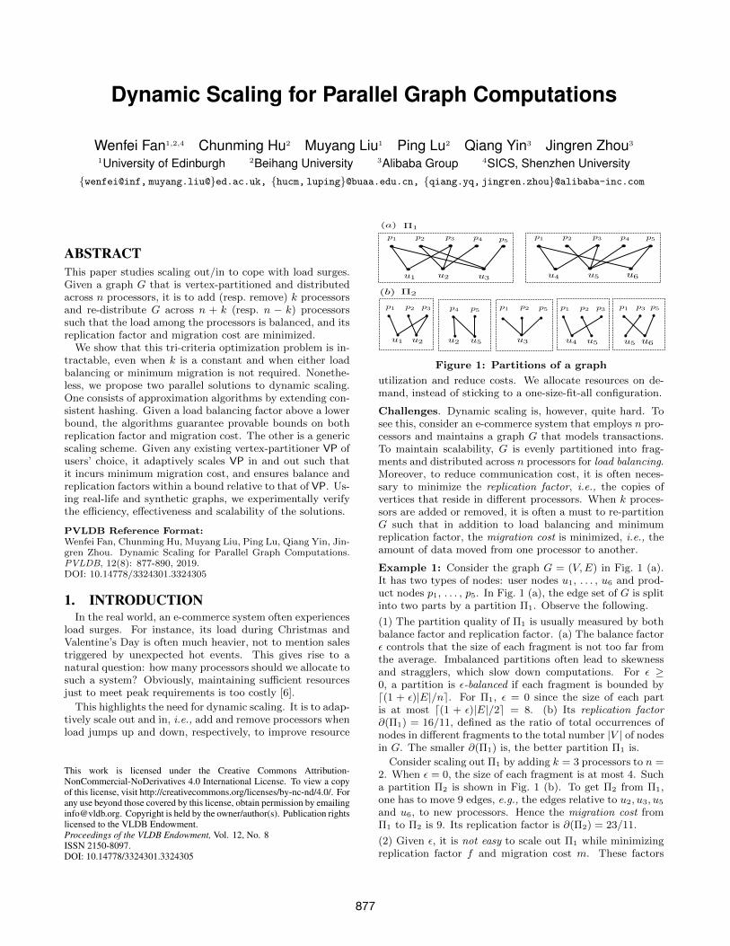
Figure 1: Partitions of a graph

utilization and reduce costs. We allocate resources on de-mand, instead of sticking to a one-size-fit-all configuration.

Challenges. Dynamic scaling is, however, quite hard. Tosee this, consider an e-commerce system that employs n pro-cessors and maintains a graph G that models transactions.To maintain scalability, G is evenly partitioned into frag-ments and distributed across n processors for load balancing.Moreover, to reduce communication cost, it is often neces-sary to minimize the replication factor, i.e., the copies ofvertices that reside in different processors. When k proces-sors are added or removed, it is often a must to re-partitionG such that in addition to load balancing and minimumreplication factor, the migration cost is minimized, i.e., theamount of data moved from one processor to another.

Example 1: Consider the graph G = (V,E) in Fig. 1 (a).It has two types of nodes: user nodes u1, . . . , u6 and prod-uct nodes p1, . . . , p5. In Fig. 1 (a), the edge set of G is splitinto two parts by a partition Π1. Observe the following.

(1) The partition quality of Π1 is usually measured by bothbalance factor and replication factor. (a) The balance factorε controls that the size of each fragment is not too far fromthe average. Imbalanced partitions often lead to skewnessand stragglers, which slow down computations. For ε ≥0, a partition is ε-balanced if each fragment is bounded byd(1 + ε)|E|/ne. For Π1, ε = 0 since the size of each partis at most d(1 + ε)|E|/2e = 8. (b) Its replication factor∂(Π1) = 16/11, defined as the ratio of total occurrences ofnodes in different fragments to the total number |V | of nodesin G. The smaller ∂(Π1) is, the better partition Π1 is.

Consider scaling out Π1 by adding k = 3 processors to n =2. When ε = 0, the size of each fragment is at most 4. Sucha partition Π2 is shown in Fig. 1 (b). To get Π2 from Π1,one has to move 9 edges, e.g., the edges relative to u2, u3, u5

and u6, to new processors. Hence the migration cost fromΠ1 to Π2 is 9. Its replication factor is ∂(Π2) = 23/11.

(2) Given ε, it is not easy to scale out Π1 while minimizingreplication factor f and migration cost m. These factors

877

interact with each other, e.g., when ε = 0, (a) to balanceload, the minimum cost is 8 (different from the cost 9 for Π2);(b) when moving 8 edges, the best f we can get is 20/11; but(c) to get an optimal f = 18/11, we need to move 12 edges.It is also nontrivial to identify which edges to be moved.

Moreover, graph G has to be re-partitioned in parallel.This is because G is already partitioned across a cluster ofmachines (e.g., by Π1 above); moreover, when G is large, itis not realistic to re-partition G by a single machine. 2

We show that dynamic scaling is NP-complete. It remainsintractable even when (a) the number k of processors addedor removed during scaling is a constant, and (b) we put norestriction on either balance factor or migration cost.

While there has been work on dynamic scaling [6, 46,42, 29, 32, 40], few of these considered how to adaptivelypartition graphs in scaling, and none offered guarantees onbalance factor, replication factor and migration cost.

One might think that incremental graph partitioners [45,37, 36, 41, 16, 30, 48, 8, 40] could be used for dynamicscaling. Given a partition P(G) of graph G and updates∆G to G, it is to compute changes ∆O to P(G) such thatP(G⊕∆G)=P(G)⊕∆O, where ⊕ applies changes ∆G (resp.∆O) to G (resp. P(G)). However, (a) the two are differentproblems: dynamic scaling is to re-partition graph G in re-sponse to addition or removal of k processors, not to changes∆G to G. Moreover, (b) in practice it is often the case thatk>n, and hence the changes ∆G and ∆O are large. It isknown that when the changes are large, incremental parti-tioning works no better than re-partitioning the entire graphG starting from scratch. Thus incremental partitioningtechniques do not apply to dynamic scaling and vice versa.

Approximation and generic methods. We propose twosolutions. There are two general approaches to graph par-titioning: edge-cut and vertex-cut. We focus on vertex-cuthere since it has not been as well studied as edge-cut.

(1) Approximate algorithms. In light of the intractability ofdynamic scaling, the best practical solution we can hope foris approximation. We develop such a solution that consistsof two approximate algorithms. Given a vertex-cut partitionΠ(n) of a graph G via hashing, balance factor ε and a num-ber k, algorithms BVC− and BVC+ scale in and out Π(n) toget a new ε-balanced partition Π(n − k) and Π(n + k), re-spectively, by extending consistent hashing. Better yet, weshow that when ε is above a small threshold, the algorithmsguarantee bounds on both replication factor f and migra-tion cost m. To the best of our knowledge, the algorithmsmake the first solution to dynamic scaling with such bounds.

(2) A scaling scheme. While the solution above offers prov-able bounds on f and m, it requires to start with an initialpartition based on hashing. Is it possible to scale an arbi-trary vertex-cut partitioner VP of users’ choice?

The answer is affirmative. We propose a generic scheme.Given an existing VP, it deduces two algorithms VP+ andVP− to scale VP out and in, respectively. We show thatthese algorithms incur minimum migration cost. Moreover,its partition quality is within a bound relative to that ofVP. That is, while the scaling scheme provides no absolutebounds like the approximate algorithms above, it providesbounds relative to VP. Hence if users have been using VP,the quality of VP+ and VP− is acceptable to them.

Contributions & Organization. Putting these together,the paper (1) formalizes the dynamic scaling problem and es-tablishes its complexity (Section 2); (2) provides an approx-imation solution with bounds on replication factor and mi-gration cost (Section 3); and (3) proposes a generic schemeto scale existing vertex-cut partitioners with low migrationcost and relative bounds on partition quality (Section 4).

(4) Experimental study (Section 5). Using real-life and syn-thetic graphs, we empirically verify the efficiency, partitionquality and scalability of our scaling algorithms. We findthe following. (a) Parallel BVC+ (resp. BVC−) algorithmoutperforms hash-based and stream-based competitors by7.4 and 19.7 (resp. 8.5 and 18.2) times in efficiency, respec-tively. (b) These algorithms also do better in replicationfactor than hash-based competitors by 1.94 and 2.04 times,up to 3.82 and 3.79 times. (c) Our generic scaling schemeis promising. Two stream-based scaling algorithms deducedunder this scheme are able to achieve partition quality asgood as re-partitioning, and are 43.8 and 40.7 times fasteron average, up to 114.7 and 132.3 times. (d) Our algorithmsscale well with large n, k and graphs; e.g., parallel BVC+

(resp. BVC−) takes 9.45s (resp. 11.37s) on graphs with 440million nodes and 14 billion edges when n = 320 and k > n

3.

This work is among the first treatments of dynamic scal-ing, from approximation to scaling of existing partitioners.

Related work. We summarize the related work as follows.

Graph partitioning. Vertex-cut was proposed in [15]. Itwas shown in [3] that it is NP-complete to minimize thereplication factor f when evenly partitioning a graph. Itis NP-hard even when the balance factor is fixed [47]. Asimple vertex-cut strategy is to assign edges to fragmentsrandomly by hashing. However, this usually leads to badlocality since it ignores the structures of input graphs [5].2DHash [44] mitigates this problem by maintaining a 2

√n−1

bound on f , where n is the number of fragments. Degree-based hash partitioning [43] assigns edges based on ver-tex degrees and favors cutting vertices with relatively largedegrees. HDRF [31] also replicates (or cuts) high-degreevertices in streaming partition. Apart from these, severalheuristics were developed, e.g., [5, 25, 47].

This work differs from the prior work in the following.

(1) As a special case of Theorem 1 (k = 0∧m =∞), we showthat vertex-cut partitioning is NP-hard even when we put noconstraint on the balance factor ε. This is analogous to itsedge-cut counterpart [14]. This is not implied by the resultsof [3, 47], and cannot be improved by further restricting ε.

Moreover, we settle the complexity of dynamic scaling andreveal what dominates the cost (Theorem 1). To the best ofour knowledge, no previous work has studied this issue.

(2) For partition quality, algorithms BVC+ and BVC− guar-antee both a bound on the replication factor and the balanceof partitions. The bound differs from the one of the degree-based approach in [43] by only a small factor, a small pricefor balancing, which is not guaranteed by [44, 43, 31, 25].

(3) BVC+ and BVC− adopt consistent hashing to prepare fordynamic scaling, which allows us to adjust an existing par-tition in response to adding or removing processors, withoutre-partitioning the graph starting from scratch. It was notstudied in the prior work [44, 15, 43, 31, 3, 47].

878

Consistent hashing. The method was proposed in [17] to re-duce the movement of hashed clients when the size of hashtable changes (see Section 3.1). As shown in [33, 27], whenthere are far more clients than servers as in real-life dynamicscaling, simple consistent hashing [17] suffers from imbal-anced load. In [27], a simple linear probing technique was in-tegrated into consistent hashing to deal with load balancing.

A popular variant is DHT (distributed hash table), e.g.,CAN [34] and Chord [38]. DHT employs consistent hashingto store key-value pairs in a distributed setting, for users tolocate a key-value pair with a given key, via “hashing”.

Closer to this work are [34, 28, 24, 18, 19] for adding or re-moving servers (analogous to fragments) in DHT, and [9, 23]for balancing the workload of servers in DHT. When addinga new server, CAN [34] bisects a randomly picked zone,which plays the same role as an “interval”, and assigns one ofthe half zones to the new server. A bucket solution was givenin [28, 24] to handle server removal, and multiple-choice al-gorithms were used in [28, 19] to add servers. Servers areevenly distributed over a unit circle for load balancing [9].Upper and lower bounds for workload are used to guide in-terval adjustments [9].

Our work differs from the prior work in the following.

(1) In contrast to [17, 27] that hash fragments, we assign thefragments in a different way to ensure that its distributionis as uniform as possible. This also helps us balance loadwhen used together with the technique of [27].

(2) We propose a strategy to add or remove fragments fordynamic scaling. (a) To add fragments, we bisect a largestinterval, rather than randomly picking one [34, 28]; (b) wedefine an order in which fragments are removed; and (c)we add or remove fragments, but do not move fragments asin [28, 24, 18]. These help us guarantee provable bounds onload balance, replication factor and migration cost.

(3) We integrate a degree-based approach [43] with consis-tent hashing, to leverage the coherence of edges (or clients)and bound the replication factor. In contrast, consistenthashing often treats all clients equally and thus ignores theircoherence. Directly adopting such approaches in our settingfails to provide a bound on the replication factor.

Scaling. The study of dynamic scaling has mostly focusedon how to allocate virtual machines (VMs) when load variesin cloud computing [6, 46, 42, 29], or how to reduce energyconsumption when workload is low [21, 22].

The scaling problems studied in the prior work differ fromDS(ε, f,m) (Section 2) in that it does not consider graphpartitioning, not to mention its three objectives (ε, f,m).

Closer to this work are [32, 40, 7, 12], which study graphpartitioning in dynamic scaling; these focus on edge-cutpartitioning. A greedy heuristic was developed in [32] tomigrate vertices when scaling; [40] randomly picks verticesbased on a given probability, and moves the vertices to otherfragments in response to changes to the graphs; [7] adoptsa lazy strategy: when a worker is added, necessary verticesare moved to it only when the worker processes a query; [12]uses a bin-packing model to balance workers after scaling.

This work differs from [32, 40, 7, 12] as follows. (a) Westudy scaling with vertex-cut partition, which is not yet wellstudied, as opposed to edge-cut. (b) None of [32, 40, 7, 12]guarantees partition quality as we do. In particular, [7] ac-cumulates vertices at new workers and is not load balanced.

2. THE DYNAMIC SCALING PROBLEMWe first state the problem and settle its complexity.

Preliminaries. We consider (un)directed graphs G =(V,E), where V is the set of vertices, and E ⊆ V × V isthe set of edges. Denote by (a) v(e) = {u,w} the set of twoend-points of an edge e, and (b) v(E′) =

⋃e∈E′ v(e) the set

of vertices that are on the edges in a set E′ ⊆ E.

Partitions. A vertex-cut n-partition of graph G = (V,E) isΠ(n) = (E1, E2, . . . , En), which partitions the edge set Einto n disjoint sets. We refer to Ei as a fragment of Π(n).

A n-partition Π(n) induces n subgraphsG1, G2, . . . , Gn ofG, where Gi = (v(Ei), Ei), such that V =

⋃i∈[1,n] v(Ei) and

E =⋃i∈[1,n]Ei. To simplify the presentation, we assume

w.l.o.g. that each Ei is nonempty in the sequel.

There are two criteria to evaluate the quality of Π(n).

(a) Balance factor. Given ε ≥ 0, Π(n) is called ε-balanced if

max{|E1|, . . . , |En|} ≤ d(1 + ε)|E|/ne.That is, no Ei is substantially larger than the average.

(b) Replication factor. The replication factor of Π(n) is

∂(Π(n))=1

|V |

n∑i=1

|v(Ei)|.

Intuitively, the larger ∂(Π(n)) is, the higher the communi-cation cost is for synchronization in a distributed setting.

Scaling. Given an integer k ∈ (−n,∞) and a n-partitionΠ(n) of G, we want to reconfigure Π(n) to a new partitionΠ(n+k). This is called scaling in if −n<k<0 by reducing |k|processors; and scaling out if k > 0 by adding k processors.

The migration cost from Π(n) to Π(n+ k) is the numberof edges moved to get Π(n+k), including (a) edges migratedfrom G1, . . . , Gn to the (new) fragments of Π(n + k), and(b) edges moved among G1, . . . , Gn+k to be rebalanced.

The dynamic scaling problem is stated as follows.

◦ Input: A n-partition Π(n) of G, an integer k > −n, abalance factor ε, a replication factor f , and a bound m.

◦ Question: Does there exist an ε-balanced vertex-cut (n+k)-partition Π(n + k) of G such that ∂(Π(n + k)) ≤ fand migration cost from Π(n) to Π(n+k) is at most m?

That is, under balance factor ε and replication factor f , itaims to minimize the migration cost of dynamic scaling.

Complexity. The dynamic scaling problem bears three cri-teria: a balance factor ε, a replication factor f and a boundm on moving cost. We denote it as DS(ε, f,m) or simply DS.

To identify the impact of the three criteria on the complex-ity, we also study three variants of DS(ε, f,m), when one ofthe three criteria is dropped. Denote by DS(f,m), DS(ε,m)and DS(ε, f) the three variants when dropping constraintson balance factor ε, replication factor f and migration costm, respectively. For example, DS(f,m) asks whether thereexists a partition Π(n+ k) of G such that ∂(Π(n+ k)) ≤ fand migration cost from Π(n) to Π(n+ k) is at most m, nolonger requiring Π(n+ k) to be load balanced.

It is not surprising that DS(ε, f,m) is NP-complete. Weshow that the intractability is quite robust: it remains NP-hard as long as f is one of the optimization goals, even whenthe number of processors added or removed is fixed.

Theorem 1: (1) Each of DS, DS(f,m) and DS(ε, f) is NP-complete, and remains NP-hard even when k is a constant.

879

(2) DS(ε,m) is in PTIME; and DS(f,m) is in PTIME whenboth k and n are fixed and when m is ∞ (unrestricted). 2

Proof: (1) An NP algorithm for DS works as follows: itfirst guesses a (n + k)-partition and then checks in PTIMEwhether the three constraints are satisfied. Hence DS is inNP, and so are its special cases DS(f,m) and DS(ε, f).

We verify the NP-hardness of DS and DS(ε, f) by reduc-tion from the 3-partition problem [2], and DS(f,m) by re-duction from the maximal clique problem (cf. [13]). Thereductions are constructed with constant k.

(2) For DS(ε,m), the PTIME algorithm below suffices. Eachtime it moves one edge from the largest fragment to a min-imum one until either (a) the balance factor gets back to ε(Yes); or (b) the migration cost exceeds the bound m (No).

When neither ε nor m is bounded and both n and k areconstants, we first show that there is a partition such that itsreplication factor is minimal, and the number of cut nodesis bounded by a constant. Based on this property, we givea PTIME algorithm for DS(f,m) with m=∞: enumerate allpossible sets of cut nodes; check whether any of the associ-ated partitions has replication factor no larger than f . 2

3. APPROXIMATION ALGORITHMSIn light of the intractability of DS(ε, f,m), the best prac-

tical solutions are approximate algorithms. We now de-velop such a solution. It consists of algorithms BVC+ andBVC− to scale out and in a partition Π(n) of a graph toan ε-balanced partition Π(n+ k), respectively (Section 3.2).Given any balance factor ε above a small threshold, bothalgorithms guarantee bounds on replication factor f andmigration cost m. We parallelize these algorithms (Sec-tion 3.3), retaining the same bounds. We are not awareof other dynamic scaling solutions that offer such bounds.

Our solution extends consistent hashing [17, 27] and hash-based partitioning [43]. We remark the following (see Sec-tion 1 for details). (1) None of the prior algorithms works ondynamic scaling, especially for deciding which fragments tobe removed or added while ensuring a bound on replicationfactor f . (2) As observed in [4, 18, 44, 33, 27], consistenthashing does no better than random hash partitioning andgives no guarantee on partition quality. (3) In particular,the algorithms of [17, 27] have no guarantee on replicationfactor f , and [43] gives no guarantee on balance factor ε.

3.1 Consistent Hashing and ExtensionWe first review consistent hashing, and then outline our

extension to cope with dynamic scaling. Consider mappingM balls to N bins. Consistent hashing [17] is a hash-stylesolution, using two different hash functions hM and hN , withthe same range. The range is modeled as a hash ring, a unitcircle C. It first hashes the balls and bins to locations onC by applying hM and hN , respectively. Each ball is thenmapped to the nearest bin on C in the clockwise order.

Its advantage is that when the number of bins changesdynamically, the number of balls that need remapping issmall. When removing a bin from C (scale in), only theballs in the deleted bin are remapped to the next bin on Cin the clockwise order. When adding a new bin on C (scaleout), it first finds certain balls that are hashed to locationsbetween the new bin and its previous bin in the clockwiseorder. It then remaps these balls to the new bin.

For dynamic scaling, we can model edges as balls and frag-ments of a partition as bins, and apply consistent hashing.However, we need to address the following challenges.

(1) Replication factor. Consistent hashing treats all ballsequally. This is equivalent to hashing edges by a randomhash function, which, as observed by [44], often leads to poorlocality. To rectify this, we employ degree-based hashingproposed in [43], which favors cutting vertices with relativelylarge degrees. Intuitively, the replication factor gets smallerwhen more vertices with large degrees are cut.

(2) Load balance. By hashing balls, a bin may have far moreballs than the others. Moreover, when M � N , the maxi-

mum load may deviate from the average by√

2M logNN

[33],

where M and N are the number of balls and bins, respec-tively. One might want to add virtual workers to mit-igate the unbalance [17], but it works only when M =O(N logN) [33]. For graph partitioning, the number of ballsis much larger than the number of bins, i.e., M � N , andadding virtual workers (a fragment is mapped to multiplepositions in circle C) cannot make the bins balanced.

To balance the workload, we enforce a given balance factoras a hard constraint, and rebalance partitions by using alinear probing technique [27]. In addition, we adopt degree-based hashing and extend consistent hashing to weightedconsistent hashing, which was not studied in [17, 27].

(3) Migration cost. Consistent hashing maps fragments asbins on the circle C by hash functions. However, when M �N , which is typically the case in our setting, this usuallyincurs heavy cost in graph partition. This is because whenballs are not distributed evenly, some bins may be overfull,and balancing the bins increases the migration cost.

To minimize the cost, we propose a fragment placementstrategy. Instead of hashing the fragments, we first evenlydistribute the fragments on the circle C [9]. When scalingin or out, our placement strategy selects fragments to be re-moved or added, and places the fragments on C as uniformlyas possible. We will see that this allows us to bound the mi-gration cost. It also helps us improve partition quality.

Notations. We will use the following notations. Considera graph G = (V,E) in which each vertex v ∈ V has a uniqueglobal id v.id. Given a unit circle C and a constant c, wedivide it into 2c segments, and use it as the hash ring. Weuse only one hash function hM that maps the id’s of verticesto the locations of C, i.e., to the set {0, 1, . . . , 2c − 1}.

We consider power-law graphs. A graph follows power-lawif the probability that a vertex has degree d is given by

Pr(d) ∝ d−α,where α is the power-law constant that controls the “skew-ness” of degree distribution. Many real-life graphs followthe power law and have a power-law constant around 2 [15].The power-law constant helps us bound replication factor,but it has no impact on the bound on migration cost.

3.2 Algorithms for Scaling Out and InWe now present algorithms BVC+ and BVC− for dynamic

scaling out and in, respectively. Given a partition Π(n) =(E1, . . . , En) of graph G and a number k > −n, BVC+ andBVC− adjust Π(n) to get a new partition Π(n + k). Asremarked earlier, the algorithms extend consistent hashing.Below we first show how to obtain an initial partition, to

880

which BVC+ and BVC− are applied. We then present ourscaling algorithms and prove the performance guarantees.

Initial partition. Given a graph G and a number n, weextend consistent hashing to compute an initial partitionΠ(n) = (E1, . . . , En) of G. In contrast to classical consistenthashing, (i) we use degree-based hashing to improve repli-cation factor; and (2) we evenly distribute the fragments onthe unit circle C to reduce migration cost. More specifically,Π(n) = (E1, . . . , En) is computed as follows.

(1) We first evenly distribute the fragments E1, . . . , En,i.e., bins, initially empty, on the circle C. This is done byallocating each Ei (i∈[1, n]) at position id 2

c−1ne on C.

(2) We then hash each edge e ∈ E by using its vertex with arelatively smaller degree. More specifically, the hash valuee.hash of an edge e = (u, v) is defined by

e.hash ={hM (v.id) deg(v) < deg(u),hM (u.id) otherwise.

This favors cutting vertices with relative large degrees. Edgee is then assigned to the nearest fragment clockwise. Morespecifically, denote by L1, L2, . . . , Ln the positions of E1,. . . , En on C respectively, we assign e to Enext par(e,C), where

next par(e, C) = argmini∈[1,n]((Li − e.hash) mod 2c).

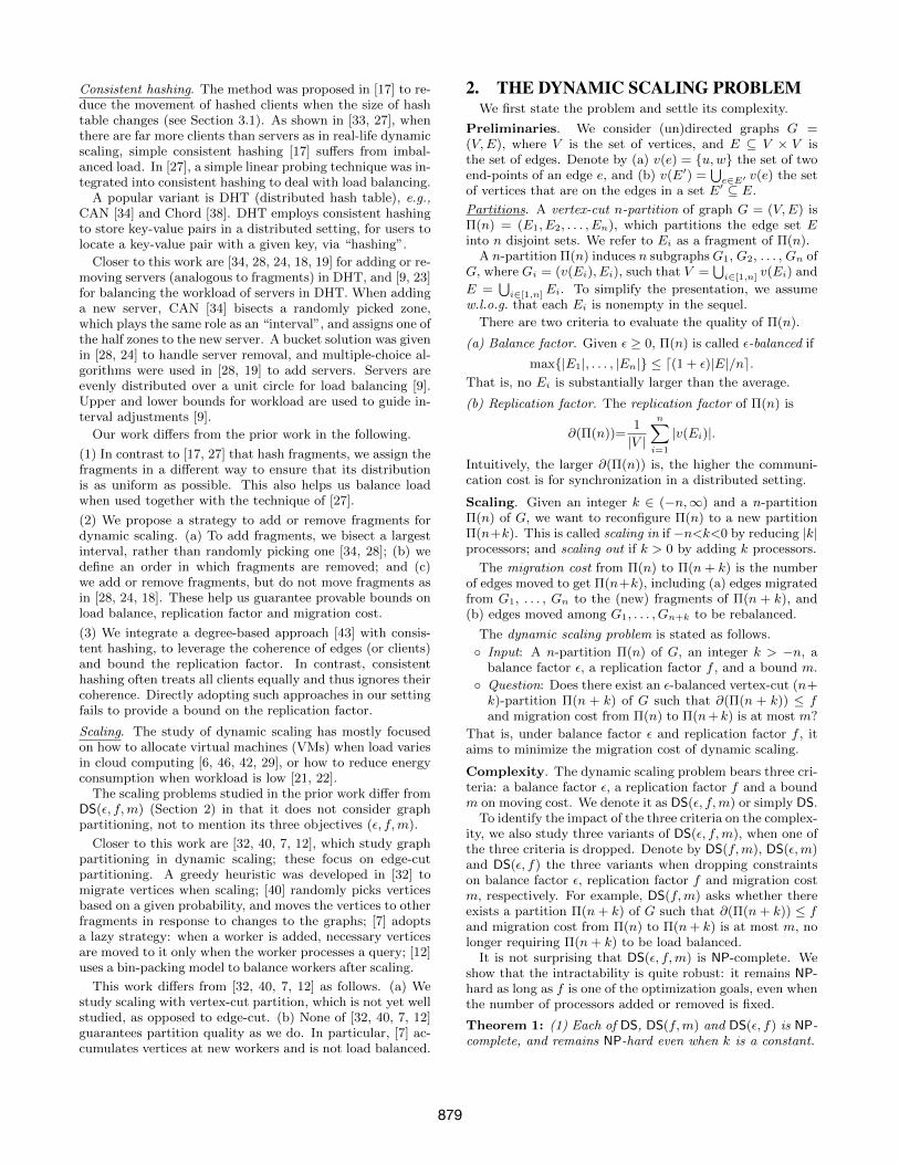
Example 2: For graph G of Fig. 1 (a), let c = 5, i.e., todivide circle C into 25 segments. Assume that hash functionhM maps vertices onto C: p1→2, p2→20, p3→22, p4→29,p5→30, u1→10, u2→12, u3→5, u4→21, u5→26, u6→25. Letn = 2, then the initial partition Π(2) = (E1, E2) obtained asabove is E1 = {e1,1, e1,3, e2,2, e2,3, e3,1, e3,2, e3,5}, and E2 ={e2,4, e4,1, e4,3, e5,2, e5,3, e5,4, e5,5, e6,1, e6,5}. 2

Overview of BVC+ and BVC−. Given a number k>− n,a balance factor ε, and a partition Π(n) that is an initialpartition obtained as above, algorithms BVC+ and BVC−

adjust Π(n) to Π(n+k) in three steps as follows.

(1) Step (1) updates fragment placement on the circle C.Suppose that for i ∈ [1, n], fragment Ei is placed at loca-tion Li before scaling starts. Given k, step (1) identifies |k|locations to remove (scale in) or add (scale out) fragments.

To minimize the migration cost in the next steps, we pro-pose a strategy to place the fragments uniformly. Let I1,. . . , In be the n intervals on C induced by E1, . . . , En, i.e.,

Ii = (Lnext(i) − Li) mod 2c

where next(i) = (i+1) mod n. Denote by Imax = max{Ii}ni=1

and Imin = min{Ii}ni=1. We select |k| locations for dynamicscaling, and ensure the following interval invariant:

Imax ≤ 2Imin, (1)

i.e., the maximum interval has size at most twice the sizeof the minimum one. As will be seen shortly, this inter-val invariant will be used to bound both migration cost andreplication factor. Note that the initial partition satisfiesthe interval invariant. Starting from an evenly distributedplacement of fragments, we will propose a strategy to main-tain the interval invariant during scaling.

(2) It then employs consistent hashing to update edge as-signments as we did in the initial partition construction.

(3) It restores balance via linear probing [27] (see below).

We will see that when ε is not too small, BVC− and BVC+

guarantee bounds on migration cost and replication factor.

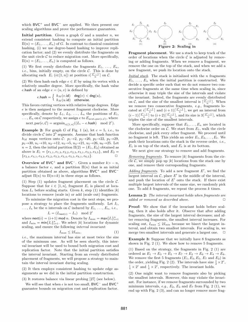
Figure 2: Scaling in

Fragment placement. We use a stack to keep track of theorder of locations when the circle C is adjusted by remov-ing or adding fragments. When we remove a fragment, weremove the one on the top of the stack, and when we add anew fragment, we push its location onto the stack.

Initial stack. The stack is initialized with the n fragmentsE1, . . . , En when the initial partition is constructed. Wedecide a specific order such that we do not remove two con-secutive fragments at the same time when scaling in, sinceotherwise it may triple the size of the intervals and violatethe invariant. Indeed, the fragments are evenly distributedon C, and the size of the smallest interval is d 2

c−1ne. When

we remove two consecutive fragments, e.g., fragments lo-cated at id 2

c−1ne and (i+ 1)d 2

c−1ne, we get an interval from

(i−1)d 2c−1ne to (i+2)d 2

c−1ne, and its size is 3d 2

c−1ne, which

triples the size of the smallest intervals.

More specifically, suppose that E1, . . . , En are located inthe clockwise order on C. We start from E1, walk the circleclockwise, and pick every other fragment. We proceed untilno fragment is left. This yields an order E1, E3, . . . , Et. Wepush their locations onto the stack in the reverse order, i.e.,E1 is on top of the stack, and Et is at its bottom.

We next give our strategy to remove and add fragments.

Removing fragments. To remove |k| fragments from the cir-cle C, we simply pop up |k| locations from the stack one byone, and remove their corresponding fragments.

Adding fragments. To add a new fragment E′, we find the

largest interval on C, place E′ in the middle of the interval,and push the location of E′ onto the stack. If there existmultiple largest intervals of the same size, we randomly pickone. To add k fragments, we repeat the process k times.

Lemma 2: The interval invariant holds when fragments areadded or removed as described above. 2

Proof: We show that if the invariant holds before scal-ing, then it also holds after it. Observe that after addingfragments, the size of the largest interval decreases; and af-ter removing fragments, the smallest interval increases. Forscaling out, Imax ≤ 2Imin because we bisect the largest in-terval, and obtain two smallest intervals. For scaling in, wemerge two smallest intervals and generate a largest one. 2

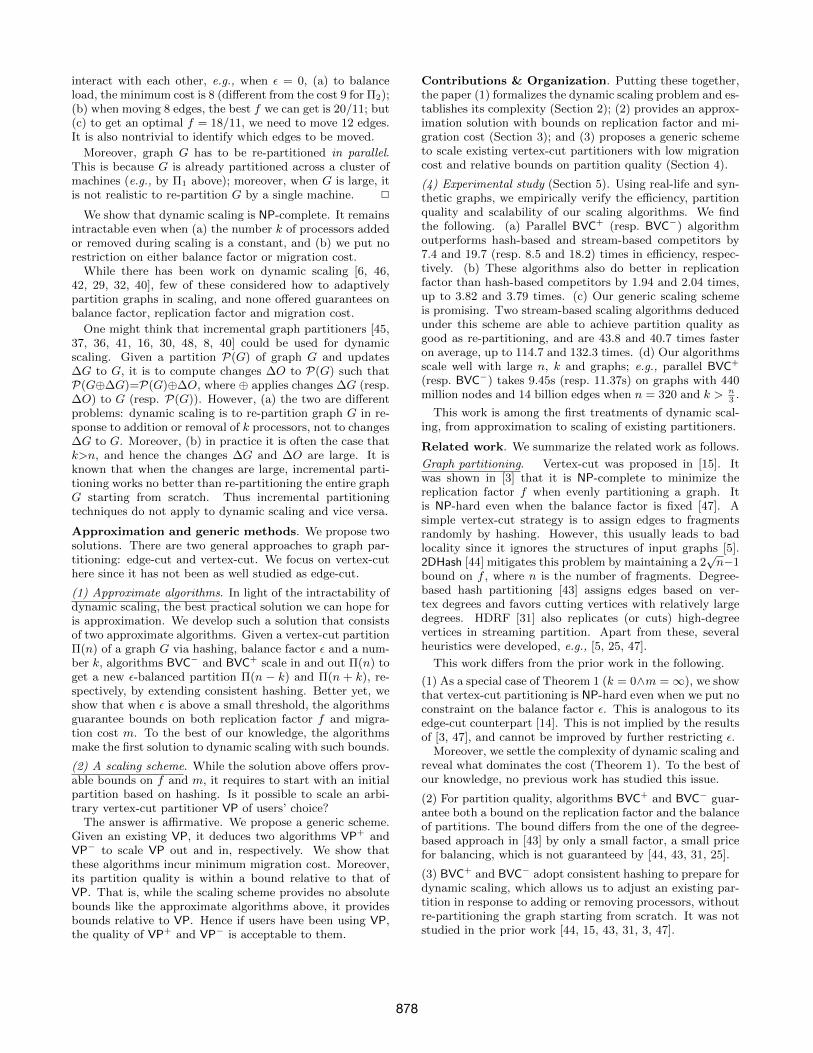
Example 3: Suppose that we initially have 8 fragments asshown in Fig. 2 (1). We show how to remove 5 fragments.

(1) Based on the strategy, the fragments in Fig. 2 (1) areordered as E1 → E3 → E5 → E7 → E2 → E6 → E4 → E8.We remove the first 5 fragments (E1, E3, E5, E7 and E2) inthe order, yielding Fig. 2 (2). The intervals have size 1

2×2c,

14× 2c and 1

4× 2c, respectively. The invariant holds.

(2) One might want to remove fragments also by pickingthe smallest intervals. However, this may violate the invari-ant. For instance, if we remove fragments surrounded by twominimum intervals, e.g., E2, E4 and E7 from Fig. 2 (1), weend up with Fig. 2 (3), and can no longer remove more frag-

881

Algorithm BVC+

Input: A partition Π(n) = (E1, . . . , En) of G,a number k > 0, and a balance factor ε.

Output: An ε-balanced new partition Π(n+ k)=(E1, . . . , En+k).

/* Step (1): Adjust fragments on C */1. identify k locations Ln+1, . . . , Ln+k for fragments to add;2. add k new fragment such that En+j at Ln+j for j ∈ [1, k];/* Step (2): Reallocate edges via consistent hashing */3. for each e ∈

⋃ni=1 Ei do

4. i∗=next par(e.hash, C); /*get the next fragment on C */5. if i∗ ∈ {n+ 1, . . . , n+ k} then6. move e to fragment Ei∗ ;/* Step (3): Balancing */

7. w ← d(1 + ε)|E|n+ke;

8. while there exists some Ei with |Ei| > w do9. ∆Ei ← select (|Ei| − w) edges from Ei;10. Ei ← Ei \∆Ei;11. next← (i+ 1) mod n;12. migrate ∆Ei to fragment Enext;13. Enext ← Enext ∪∆Ei;

Algorithm BVC−

Input: A partition Π(n) = (E1, . . . , En) of G,a number 0 < k < n, and a balance factor ε.

Output: A new partition Π(n) = (E′1, . . . , E′n−k) of G.

1. identify and remove fragments Ej1 , . . .Ejk , with a stack;

2. for each edge e ∈⋃ki=1{Eji} do

3. i = next par(e.hash, C); /*get the next fragment on C */4. move e to Ei;5. {E′1, E′2, . . . , E′n−k} ← {E1, . . . , En} \ {Ej1 , . . . , Ejk};6. balance E′1, . . . , E

′n−k by linear probing as Algorithm BVC+;

Figure 3: Algorithm for scaling out/in

ment without violating the invariant. Indeed, if we furtherremove E1, we end up with Fig. 2 (4), in which the distancebetween E8 and E3 triples the distance between E5 and E6.Removing other fragments also inflicts violation. 2

We now present algorithms BVC+ and BVC− in Fig. 3.

Algorithm BVC+ Given Π(n), ε and k > 0, BVC+ extendsΠ(n) to Π(n+ k) in three steps. (1) It first adds new frag-ments on circle C as remarked earlier, maintaining the inter-val invariant. (2) It then re-allocates edges by a degree-basedapproach to improve locality, and maps edges to fragmentsas in consistent hashing. (3) Finally it adjusts the partitionto make it balanced. Steps (2) and (3) integrate consistenthashing [17, 27] and the degree-based approach [43].

(1) It first identifies k locations with the placement strategyabove, and adds k new fragments at the locations (lines 1-2).

(2) It then identifies edges belonging to the new fragmentsbased on consistent hashing and moves them to the corre-sponding new fragments (lines 3-6).

(3) Finally, it applies linear probing [27] to balance the par-tition (lines 7-13). For each fragment Ei, if it is not balanced

(|Ei|>d(1+ε) |E|n+ke), then it forwards |Ei|−d(1+ε) |E|

n+ke

edges to the next fragment in the clockwise order.

Remark. (a) BVC+ terminates when all fragments are bal-anced. This is assured by that each edge is migrated at mostn+ k times, and at most |E| edges need to be moved.

(b) The initial partition step can be done by BVC+, denotedby BVC. Indeed, it is a special case when the graph is givenas a fragment, and BVC+ adds another n− 1 fragments.

Example 4: We show how BVC+ extends the partition Π(2)of Example 2 to a new partition Π(5) = (E1, . . . , E5). It first

Figure 4: Scaling out

identifies 3 locations on circle C to place the new fragmentsE3, E4 and E5. It then finds edges that belong to the newfragments, and moves them to the right place. We get E1 ={e1,1, e1,3, e2,2, e2,3}, E2 = {e2,4, e5,4, e5,5}, E3 = {e3,1, e3,2,e3,5}, E4 = {e4,1, e4,3, e5,2} and E5 = {e5,3, e6,1, e6,5}. Thisyields balanced Π(5) of Fig. 1 (b). 2

Algorithm BVC− Given a balance factor ε, a number k suchthat −n<k<0, and a partition Π(n) = (E1, . . . , En) of Gsuch that Ei’s are placed on a unit circle C, BVC− adjustsΠ(n) to Π(n+k) as follows. It first identifies |k| fragmentsEj1 , . . . , Ej|k| on the top of the stack, and removes them

from circle C (line 1). As assured by Lemma 2, after theremoval, the circle C still satisfies the interval invariant.

After these steps, BVC− remaps the edges in Ej1 , . . . ,Ej|k| to the remaining fragments based on consistent hashing

(lines 2-4). More specifically, for each edge e in a removedfragment, it finds the next fragment on C in the clockwiseorder (line 3) and moves e to it (line 4). At last it balancesthe fragments via linear probing as in BVC+ (lines 5-6).

Analysis. We show that when the balance factor is not toosmall, BVC+ and BVC− guarantee bounds on both replica-tion factor and migration cost. Since each edge is hashed byits vertices, denote by hmax the maximum number of times ofa vertex used for hashing. Here hmax is usually much smallerthan the maximum degree of the graph, as for a vertex it isunlikely that most of its edges are hashed using its id.

Given k>−n, we have the following starting from an ini-tial partition with BVC+, in which β1

k= 8(n+k)hmax

|E| log((n+

k)√|E|+ 1), βk=

√β1k(√β1k+√

2), and θ = dmin × α−1α−2−

dmin × α−12α−3

+ 12, where dmin is the minimal node degree in

a power-law graph, and α is its power-law constant [43].

Theorem 3: If k > −n and ε > 1 + 2βk, then (1) theexpected value of migration cost when scaling out (resp. in)from Π(n) to Π(n + k) via BVC+ (resp. BVC−) is at most

O(k |E|n+k

) (resp. O(k |E|n

)); and (2) the expected value of the

replication factor is at most (n+k)(1−(1−2 1n+k

)θ)+ 2|V | . 2

Observe the following about Theorem 3.

(1) The lower bound βk for balance factor is not very restric-tive, since in the real world it is common to find that |E|�n.Taking Twitter as an example (see Section 5), βk≤0.009 forn=64, where |E| is approximately 1.5 billion.

(2) Edge selection in linear probing affects neither migrationcost [27] nor the upper bound for replication factor.

(3) The bound for migration cost holds on general graphs,but not the replication factor fe. On a power-law graph G,fe of degree-bashed hashing would decrease when G getsmore skewed [43]; this does not hold on general graphs.

Proof: We only give a proof sketch for the bounds forBVC−; the proof for BVC+ is similar.

(1) The migration cost of BVC− includes (a) the cost of mov-ing edges from removed fragments to fragments that remain;and (b) the cost of rebalancing fragments. For cost (a), since

882

each fragment has at most d(1 + ε) |E|ne edges, and k frag-

ments are removed, at most O(k |E|n

) edges are migrated.

Thus the migration cost for (a) is bounded by O(k |E|n

).For cost (b), we show that the expected number of edges

in each fragment Ei to be forwarded is bounded by O( 1n2 ),

by using Bernstein’s inequality [10]. Since each edge can beforwarded at most n times, the migration cost for balancingeach fragment is at most O( 1

n). Hence total migration cost

for balancing all n fragments is bounded by O(1).

(2) Suppose that Vi is the set of vertices contained in frag-ment Ei (i ∈ [1, n+k]) after BVC− terminates. To bound thereplication factor, by its definition, we only need to boundthe expected value of |Vi| for all i ∈ [1, n + k]. Note that|Vi| can be bounded by the number of vertices hashed to Eiplus the number of vertices forwarded to Ei during the re-balancing step. The number of vertices hashed to Ei can bebounded by |E|(1− (1− 2

n+k)θ) using the technique of [43],

since the fragments are such placed that the invariant holds,and the probability that an edge is hashed to Ei is boundedby 2

n+k. For the number of vertices forwarded to Ei, since

the total number of forwarded edges is bounded by O(1) asproved above, and each edge has two associated vertices, thenumber of vertices forwarded to Ei can also be bounded. 2

3.3 ParallelizationDynamic scaling has to be conducted in parallel. It starts

with a partition when a graph is already fragmented anddistributed across a cluster of processors. To scale out/in,all processors involved need to work together in parallel.Moreover, when dealing with large graphs, it is not practicalfor a single-machine to compute a balanced partition.

In light of this, we next parallelize BVC+ and BVC−, anddevelop their parallel versions ParBVC+ and ParBVC−, re-spectively. We show that these parallel algorithms retain thesame performance guarantees as their serial counterparts.

Parallel setting. Our parallel algorithms run in a shared-nothing distributed setting, as commonly used nowadays.

(a) Initially, a graph G = (V,E) is partitioned into n frag-ments E1,. . . , En, which are distributed to n processors P1,. . . , Pn, respectively, referred to as workers.

(b) The workers run under the BSP model [39], which sep-arates scaling into supersteps. In a superstep, each workerconducts computation of ParBVC+ or ParBVC− to refine itsown fragment and exchanges updates via messages.

(c) When adding or deleting |k| fragments (k>−n), |k| addi-tional workers are added or |k| existing workers are deleted.

Parallel algorithms. We only present ParBVC+; ParBVC−

is similar. As opposed to its serial counterpart (Section 3.2),the algorithm conducts in parallel (a) the computation ofhash values and edge assignments, and (b) edge migrationand linear probing for load balancing, by all workers.

Algorithm ParBVC+. Given a partition Π(n) of G placedon a unit circle C, a balance factor ε and a number k > 0,ParBVC+ scales out Π(n) to an ε-balanced partition Π(n+k).Like BVC+, it first adds k new fragments on the circle C,maintaining the interval invariant. It then identifies edgesthat belong to the new fragments by consistent hashing, andmigrates them to the corresponding fragments. As opposedto BVC+, ParBVC+ does these in parallel : for each existingfragment Ei (1 ≤ i ≤ n), its worker Pi identifies and moves

out the related edges in Ei. Finally ParBVC+ balances theresulting partition, in parallel via linear probing.

Analysis. We show that ParBVC+ retains the same boundson replication and migration cost as BVC+ (Theorem 3).

(a) Bounds for ParBVC+. Since ParBVC+ and BVC+ usethe same hash function for edges, the distribution of edgesamong fragments is the same for both ParBVC+ and BVC+.Moreover, both algorithms maintain the same interval in-variant (Lemma 2). Hence the same bounds of Theorem 3can be deduced for both of them, although ParBVC+ mi-grates edges in parallel, while BVC+ does it sequentially.

(b) Running time. For BVC+, the migration cost is bounded

by O(|k| |E|n+k

). For ParBVC+, the expected running time is

in O( |E|n+k

), since edge migration from existing fragments to

new ones dominates the cost, and ParBVC+ conducts it inparallel. By Theorem 3, only a small number of edges needto be moved in the linear probing step for rebalancing.

4. A GENERIC SCALING SCHEMEThe approximation solution above requires an initial par-

tition that places fragments on a hash ring and satisfies theinterval invariant. In practice, however, users often startwith a partition computed by a partitioning algorithm VPof their own choice. Is there a method that scales any exist-ing vertex-cut partitioner VP in response to load surges?

We next develop such a generic solution and show thatit guarantees minimum migration cost and a relative boundon partition quality (Section 4.1). As proof of concept, wescale two existing vertex-cut partitioners (Section 4.2).

4.1 Dynamic Scaling SchemeGiven a vertex-cut partitioning algorithm VP, we deduce

algorithms VP+ and VP−. Given a n-partition Π(n) =(E1, . . . , En) generated by VP and an integer k > −n, VP+

and VP− compute partition Π(n+ k) for scaling out and in,respectively, depending on whether k > 0. To simplify thepresentation, we assume w.l.o.g. that ε = 0 in this section.

Scaling scheme. The scheme computes Π(n+k) by select-ing a minimum number of edges to move, employing VP tore-assign these edges, and retaining the edge assignments ofVP as much as possible. This allows us to minimize migra-tion cost and achieve partition quality comparable to VP.More specifically, VP+ and VP− work as follows.

Scaling out. From each fragment Ei (i ∈ [1, n]), VP+ (a)

selects a subset E′i ⊆ Ei of edges such that |E′i| = k|Ei|n+k

, and

(b) applies VP to the set⋃ni=1E

′i of all selected edges, and

obtains a k-partition (E′′n+1, . . . , E′′n+k). (c) These yield a

(n+ k)-partition (E1 \ E′i, . . . , En \ E′n, E′′n+1, . . . , E′′n+k).

That is, it employs the original partitioner VP to re-assignthe selected edges. It only moves edges from Ei to the k newfragments, not between existing fragments Ei (i ∈ [1, n]).

Scaling in. VP− randomly selects |k| fragments Ei1 , . . . ,Ei|k| to remove, and then employs VP to reassign edges of⋃|k|j=1Eij to the remaining fragments Ej1 , . . . , Ejn+k .

VP+ and VP− incur the minimum migration cost, sincethey move the minimum number of edges to make the newpartition balanced with ε = 0. VP+ only moves edges fromoriginal fragments to newly added ones, and VP− reassigns

883

edges from the removed fragments to the remaining ones.Neither moves edges among existing fragments.

Proposition 4: Given a balanced partition Π(n), the mi-

gration cost of VP+ (resp. VP−) is O( k|E|n+k

) (resp. O( |k||E|n

))

when adding (resp. removing) |k| fragments. 2

Edges selection. We next show that the algorithms alsooffer relative bounds on replication factor f . Below we focuson VP+; the analysis of VP− is similar and simpler.

Observe that VP+ only selects edges from overfull frag-ments and moves them to newly added ones. VP+ uses thefollowing edge selection strategy: from each fragment Ei(i ∈ [1, n]), VP+ selects k

n+k|Ei| edges from Ei such that

the number of vertices on the selected edges is minimum.We now give an upper bound on the replication factor of

VP+. Denote by τi the average vertex degree in fragment Ei.

Proposition 5: The replication factor after VP+ is at mostF+k· k

n+k2|E|

min{τi}ni=1·|V |with the edge selection strategy above.

Here min{τi}ni=1 is the minimum average vertex degree of allfragments, and F is the replication factor before scaling. 2

Proof: This is deduced from the following: (a) the repli-cation factor of the original fragments after the scaling isat worst F ; (2) the number of vertices on selected edges

from fragment Ei is at most kn+k

2|Ei|τi

; and (3) each selectedvertex can be assigned to at most k new fragments. 2

In practice, the replication factor is expected to be betterthan this upper bound, because (1) when we remove edgesfrom a fragment Ei, its replication factor is decreased and isoften smaller than F ; and (2) when we use VP to distributethe selected edges, the replication factor of the new frag-ments is often smaller than the second term in Proposition 5,since each vertex unlikely appears in all new fragments.

4.2 Scaling Stream PartitionersAs case studies, we next scale HDRF [31] and Greedy (Pow-

ergraph [15]), two well-known vertex-cut partitioners.Both partitioning algorithms are stream-based, which pro-

cesses edges in a one-pass fashion. Consider a vertex-cutpartition Π(n) = (E1, . . . , En) generated so far. An incom-ing edge e is assigned to a fragment Ei based on scoresS(e, Ei)(i ∈ [1, n]), which aggregates edges assigned to Eiso far. More specifically, edge e is assigned to Ei∗ , where

i∗ = argmaxi∈{1,...,n}S(e, Ei),

i.e., the fragment that maximizes the score. PartitionersHDRF and Greedy use different score functions.

HDRF. We start with HDRF, which favors replicating ver-tices with relatively large degrees. Given an edge e = (u, v),it computes a score S(u, v, Ei) w.r.t. each fragment Ei:

S(u, v, Ei) = SRep(u, v, Ei) + SBal(Ei), (2)

where SRep(u, v, Ei) is a replication score of e w.r.t. Ei andSBal(Ei) is a balance score of Ei, defined as follows. Toreplicate vertices with higher degrees first, HDRF definesSRep(u, v, Ei) = g(u, v, Ei) + g(v, u, Ei), where

g(v, u, Ei) =

{1 + deg(u)

deg(v)+deg(u)if v ∈ Vi,

0 otherwise.

Here deg(u) and deg(v) are the degrees of u and v, respec-tively. Let Maxsize and Minsize be the maximum and

minimum size of all fragments when processing edge e, re-spectively, then the balance score SBal(Ei) of e is defined as

SBal(Ei) = λMaxsize− |Ei|

1 + Maxsize−Minsize,

where λ is a user-defined parameter that controls the impactof the balance score. HDRF sets the default value of λ as 2.

Edge selection of HDRF. We focus on edge selection forscaling out, since there is no much flexibility for scaling in.A naive method is to randomly select edges from overfullfragments. However, this usually leads to degeneration ofpartition quality. Instead, we introduce two strategies basedon score and timestamp of stream HDRF.

(1) Score based. Intuitively, a larger HDRF score S(e, Ei) ofe indicates better locality of e w.r.t. fragment Ei. Henceit is natural to move out edges with relatively lower scores.However, we cannot simply use the score assigned to e whenit comes in, since it only reflects the fragment informationat that moment. Hence for each edge e, we compute a newscore S(e, Ei \ {e}) by treating e as a new edge for Ei. Edgeswith relatively lower new scores are selected for scaling out.

(2) Timestamp based. Intuitively, edges that are processedearlier are more likely to be assigned to “wrong” fragments,since their scores are computed with less information andmay not be accurate. In HDRF, deg(u) and deg(v) used inthe score function cannot be computed in advance and thusare approximated by their partial degrees, i.e., the numberof processed edges that are attached to u and v, respectively.The degrees used in the score computation for earlier edgesare not as accurate as those of later edges.

This suggests that we revise the assignment of early com-ing edges and retain the assignment of later ones. Hencewhen running HDRF, we associate with each edge e a times-tamp recording when it is added to its fragment. We selectedges with relatively smaller timestamp for scaling out.

Based on these, we deduce HDRF+ and HDRF− as follows.

HDRF+. From each fragment Ei, HDRF+ selects kn+k|Ei|

edges based on one of the edge selection strategies above. Itmerges these edges as a new stream and invokes HDRF toassign these edges to the k newly added fragments.

HDRF−. This case is simpler. HDRF− randomly selects |k|fragments and merges their edges as a new stream. It thenuses HDRF to reassign the edges to the remaining fragments.

As will be demonstrated in Section 5, HDRF+ and HDRF−

scale partition with quality comparable to re-partitioningthe entire graphs by HDRF starting from scratch, while theyincur the minimum migration cost (Proposition 4).

Replication factor. We show that with the two simple edge-

selection strategies above, HDRF+ still guarantees boundedreplication factor relative to partitioner HDRF.

We use the following notations. Denote by (a) E′1, . . . , E′n

the sets of edges selected from partition (E1, . . . , En) by oneof the strategies; (b) E′′1 , . . . , E

′′n the edges remaining in the

n fragments; and (c) f ′ and f ′′ the replication factor of(E′1, . . . , E

′n) and (E′′1 , . . . , E

′′n), respectively.

Observe that f ′′ is at least as good as the replication factorof the original (E1, . . . , En). For the k new fragments, weshow that the replication factor is comparable to f ′. Tosimplify the analysis, we adopt λ = 1 as in [31].

884

Proposition 6: The replication factor after HDRF+ is

bounded by (1) f ′′+ 2k2

n+k|E| with the score-based strategy, and

(2) f ′+f ′′+ kn+k

|E||V |−

|V1|2·|V | for timestamp-based when λ = 1,

where V1 is the number of vertices in the selected edges. 2

Proof: We verify statement (1); the proof for statement (2)is similar. Observe that the replication factor of the re-sulting partition is the sum of the replication factor of nremaining fragments Π(n)′ = (E′′1 , . . . , E

′′n) and that of the

partition Π(k) of k new fragments with edges E′1, . . . , E′n.

The replication factor of Π(n)′ is at worst f ′′. From a de-tailed analysis of the new score S(e, Ei \ {e}) it follows that

the replication factor of Π(k) is bounded by 2k2

n+k|E|. 2

Greedy. Greedy is a stream-based partitioner adopted byPowergraph [15]. It can be seen as a special case of HDRF.It also uses Eq. (2) to compute edge scores. It differs fromHDRF in that it (a) uses 1 as the default value for λ tobalance score; and (b) it does not include the impact ofdegrees in the replication score and defines g(v, u,Ei) by

g(v, u,Ei) =

{1 if v ∈ Vi,0 otherwise.

The edge selection strategies for HDRF also work for Greedy.Denote by Greedy+ and Greedy− the scaling algorithmsdeduced from Greedy along the same lines. Then the boundsfor migration cost and replication factor of HDRF+ andHDRF− also hold on Greedy+ and Greedy−, respectively.

Parallelization. Following [35], we parallelize HDRF+ andHDRF− (resp. Greedy+ and Greedy−) in a mini-batch fash-ion as follows. Each worker maintains a shared state that in-cludes the information of degrees and locations of processedvertices. The edge assignment is conducted in rounds. In around, each worker handles a small batch of edges in paral-lel, as in HDRF or Greedy; workers communicate with eachother at the end of each round to synchronize the sharedstate. The process terminates when all edges are processed.

5. EXPERIMENTAL STUDYUsing real-life and synthetic graphs, we conducted four

sets of experiments to evaluate our scaling algorithms fortheir (1) efficiency, (2) partition quality, (3) scalability, and(4) impact on the performance of graph analysis tasks.

Experimental setting. We start with the setting.

Datasets. We used three real-life power-law graphs: (a) PLD[26], an undirected graph with 39 million nodes and 623 mil-lion edges, in which each node represents a pay-level domainand each edge indicates a hyperlink between a pair of do-mains; (b) Twitter [20], a social network with 42 millionusers and 1.5 billion links; and (c) UKWeb [1], a large Webgraph with 106 million nodes and 3.7 billion edges.

We also generated synthetic graphs with size up to 440million vertices and 14 billion edges, to test scalability.

Algorithms. We implemented approximate ParBVC− and

ParBVC+ (Section 3), and parallel HDRF+, HDRF−, Greedy+

and Greedy− (Section 4), all in C++, compared with thefollowing: (1) CH [17], a consistent-hashing partitioner; incontrast to ParBVC+ and ParBVC−, CH takes edge id ashashing key and hashes fragments to a unit circle; it alsouses a virtual-sever method to balance load; (2) 2DHash [44],a widely used hash-based vertex partitioner; (3) Libra [43],

a state-of-the-art degree-based hashing algorithm; and (4)stream partitioners HDRF and Greedy (Section 4). Since2DHash, Libra, HDRF and Greedy do not support dynamicscaling, we mainly consider their partition quality.

To evaluate the effectiveness of our edge selection strate-gies of our generic scaling scheme, we implemented variantsof HDRF+ and Greedy+, also in C++. Denote by HDRF+

s

and HDRF+t the implementations of HDRF+ with edge selec-

tion based on score and timestamp, respectively; similarlyfor Greedy+s and Greedy+t . The results reported for HDRF+

and Greedy+ take the average of two strategies. We also im-plemented a strategy that randomly chooses edges for scal-ing out, denoted by HDRF+

r and Greedy+r , respectively. Weparallelized the algorithms as described in Section 4.2. Themini-batch size is set to 256 by default.

The experiments were conducted on GRAPE, a parallelgraph processing engine [11], deployed on an HPC clusterof up to 36 machines, each with 12 cores powered by IntelXeon 2.2GHz and 128GB memory, with a 10Gbps linkbetween machines. Each experiment was repeated 5 timesand the average is reported here.

Experimental results. We next report our findings.

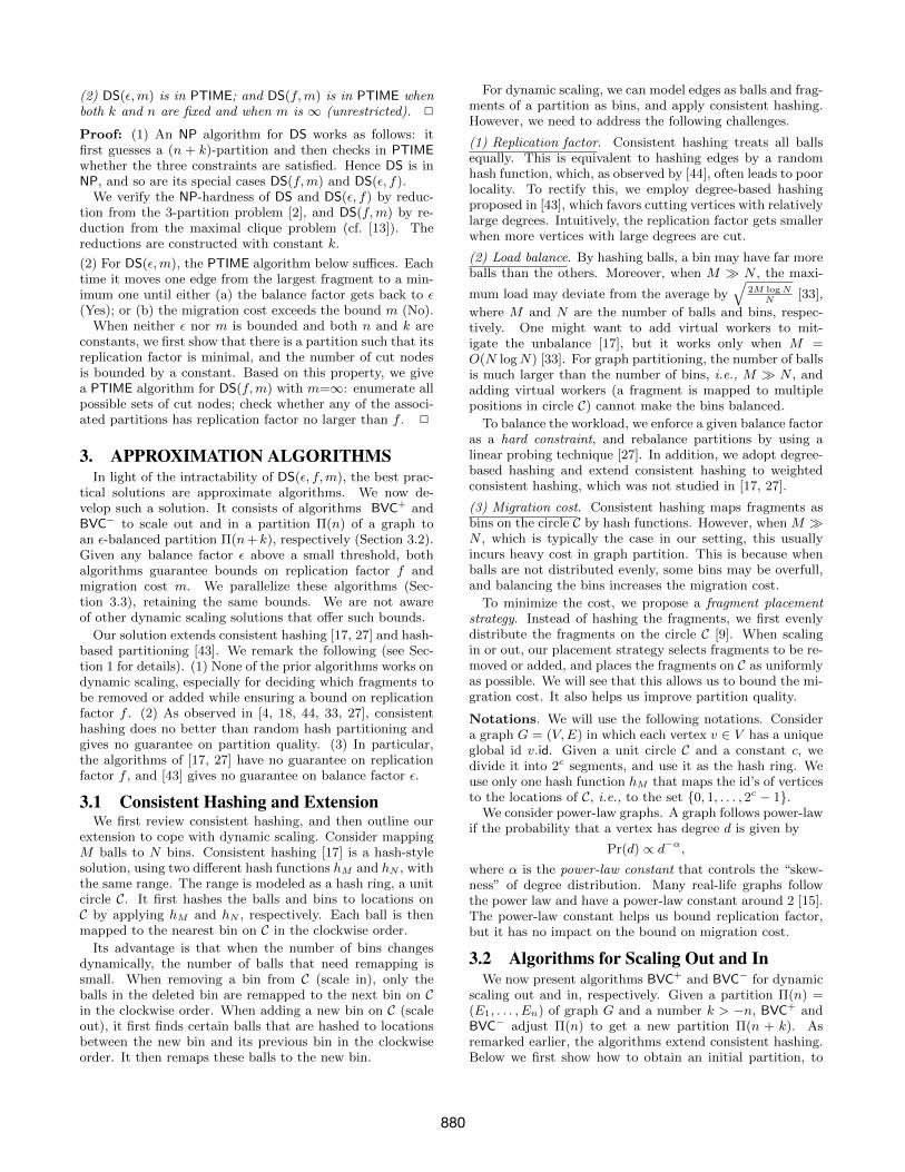
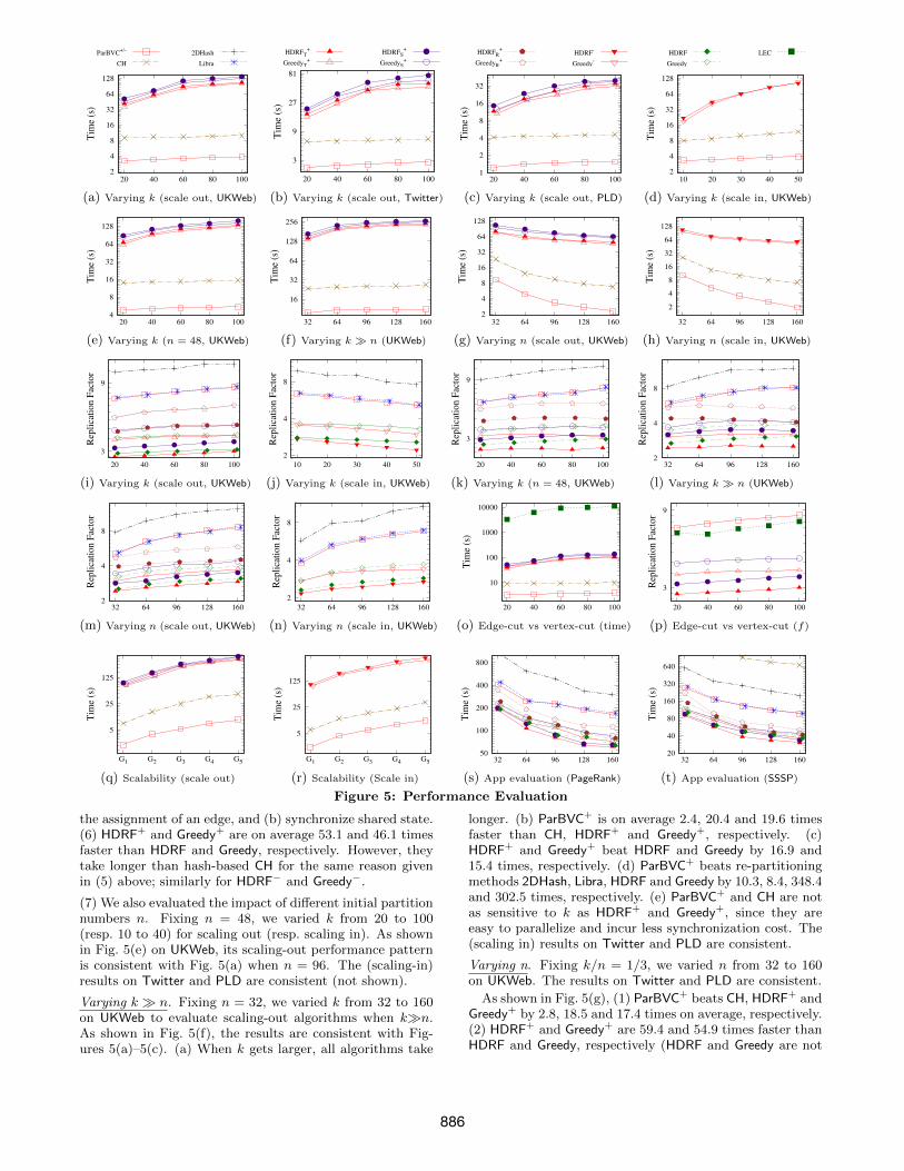
Exp-1: Efficiency. We first evaluated the scaling timeand migration cost of the algorithms. For ParBVC+ andParBVC−, we set balance factor ε = 0.1; the other algorithmsdo not take ε as a hard constraint on load balance.

Varying k. Fixing n = 96, we varied k from 20 to 100 (resp.10 to 50) for scaling out (resp. in). We find the following.

(1) As shown in Figures 5(a)-5(c), ParBVC+ performs thebest in time efficiency. It outperforms CH, HDRF+ andGreedy+ by 2.7, 20.3 and 18.5 times, respectively, up to 3.4,36.1 and 33.1 times. All algorithms take longer when k getslarger, as expected. However, ParBVC+ and CH are lesssensitive to the change of k than HDRF+ and Greedy+, sincethey incur less synchronization overhead during scaling.

(2) 2DHash, Libra, HDRF and Greedy do not supportdynamic scaling, and have to re-partition graphs. ParBVC+

is 8.9, 7.4, 926.5 and 763.6 times faster than these methods,respectively, up to 13.1, 11.2, 1406.8 and 1224.8 times (notshown). This is because the re-partitioning methods need to(a) recompute edge assignments, and (b) move most edges(their migration cost is 2.9 times larger than ParBVC+).

(3) The results for scaling in are consistent with scaling out.As shown in Fig. 5(d), on average ParBVC− outperforms CH,HDRF− and Greedy− on UKWeb by 2.7, 18.6 and 17.4 times,respectively, up to 3.1, 26.7 and 27.8 times. The results onTwitter and PLD are consistent (not shown).

(4) CH incurs larger migration cost, on average 1.1 (resp. 1.2)times more than ParBVC+ (resp. ParBVC−). It is 2.7 (resp.2.7) times slower than ParBVC+ (resp. ParBVC−) (see (1)),since CH generates unbalanced partitions (Exp-2), whichyield stragglers and slow down scaling. This verifies the ef-fectiveness of our fragment placement strategy (Section 3.2).

(5) HDRF+ and Greedy+ (resp. HDRF− and Greedy−) incurminimum migration cost. These are 1.37 and 1.37 (resp. 1.40and 1.40) times better than ParBVC+ (resp. ParBVC−) onaverage, respectively. Nevertheless, they are slower thanParBVC+ and ParBVC−. This is because during scaling theyneed to (a) compute the score w.r.t. all fragments to decide

885

ParBVC+/-

CH

2DHash

Libra

HDRFT+

GreedyT+

HDRFS+

GreedyS+

HDRFR+

GreedyR+

HDRF-

Greedy-

HDRF

Greedy

LEC

2

4

8

16

32

64

128

20 40 60 80 100

Tim

e (s

)

(a) Varying k (scale out, UKWeb)

3

9

27

81

20 40 60 80 100

Tim

e (s

)

(b) Varying k (scale out, Twitter)

1

2

4

8

16

32

20 40 60 80 100

Tim

e (s

)

(c) Varying k (scale out, PLD)

2

4

8

16

32

64

128

10 20 30 40 50

Tim

e (s

)

(d) Varying k (scale in, UKWeb)

4

8

16

32

64

128

20 40 60 80 100

Tim

e (s

)

(e) Varying k (n = 48, UKWeb)

16

32

64

128

256

32 64 96 128 160

Tim

e (s

)

(f) Varying k � n (UKWeb)

2

4

8

16

32

64

128

32 64 96 128 160

Tim

e (s

)

(g) Varying n (scale out, UKWeb)

2

4

8

16

32

64

128

32 64 96 128 160

Tim

e (s

)

(h) Varying n (scale in, UKWeb)

3

9

20 40 60 80 100

Rep

lica

tio

n F

acto

r

(i) Varying k (scale out, UKWeb)

2

4

8

10 20 30 40 50

Rep

lica

tio

n F

acto

r

(j) Varying k (scale in, UKWeb)

3

9

20 40 60 80 100

Rep

lica

tio

n F

acto

r

(k) Varying k (n = 48, UKWeb)

2

4

8

32 64 96 128 160

Rep

lica

tio

n F

acto

r

(l) Varying k � n (UKWeb)

2

4

8

32 64 96 128 160

Rep

lica

tio

n F

acto

r

(m) Varying n (scale out, UKWeb)

2

4

8

32 64 96 128 160

Rep

lica

tio

n F

acto

r

(n) Varying n (scale in, UKWeb)

10

100

1000

10000

20 40 60 80 100

Tim

e (s

)

(o) Edge-cut vs vertex-cut (time)

3

9

20 40 60 80 100

Rep

lica

tio

n F

acto

r

(p) Edge-cut vs vertex-cut (f)

5

25

125

G1 G2 G3 G4 G5

Tim

e (s

)

(q) Scalability (scale out)

5

25

125

G1 G2 G3 G4 G5

Tim

e (s

)

(r) Scalability (Scale in)

50

100

200

400

800

32 64 96 128 160

Tim

e (s

)

(s) App evaluation (PageRank)

20

40

80

160

320

640

32 64 96 128 160

Tim

e (s

)

(t) App evaluation (SSSP)

Figure 5: Performance Evaluation

the assignment of an edge, and (b) synchronize shared state.(6) HDRF+ and Greedy+ are on average 53.1 and 46.1 timesfaster than HDRF and Greedy, respectively. However, theytake longer than hash-based CH for the same reason givenin (5) above; similarly for HDRF− and Greedy−.

(7) We also evaluated the impact of different initial partitionnumbers n. Fixing n = 48, we varied k from 20 to 100(resp. 10 to 40) for scaling out (resp. scaling in). As shownin Fig. 5(e) on UKWeb, its scaling-out performance patternis consistent with Fig. 5(a) when n = 96. The (scaling-in)results on Twitter and PLD are consistent (not shown).

Varying k � n. Fixing n = 32, we varied k from 32 to 160on UKWeb to evaluate scaling-out algorithms when k�n.As shown in Fig. 5(f), the results are consistent with Fig-ures 5(a)–5(c). (a) When k gets larger, all algorithms take

longer. (b) ParBVC+ is on average 2.4, 20.4 and 19.6 timesfaster than CH, HDRF+ and Greedy+, respectively. (c)HDRF+ and Greedy+ beat HDRF and Greedy by 16.9 and15.4 times, respectively. (d) ParBVC+ beats re-partitioningmethods 2DHash, Libra, HDRF and Greedy by 10.3, 8.4, 348.4and 302.5 times, respectively. (e) ParBVC+ and CH are notas sensitive to k as HDRF+ and Greedy+, since they areeasy to parallelize and incur less synchronization cost. The(scaling in) results on Twitter and PLD are consistent.

Varying n. Fixing k/n = 1/3, we varied n from 32 to 160on UKWeb. The results on Twitter and PLD are consistent.

As shown in Fig. 5(g), (1) ParBVC+ beats CH, HDRF+ andGreedy+ by 2.8, 18.5 and 17.4 times on average, respectively.(2) HDRF+ and Greedy+ are 59.4 and 54.9 times faster thanHDRF and Greedy, respectively (HDRF and Greedy are not

886

shown). (3) When n is larger, all algorithms take less time.(4) HDRF+ and Greedy+ are not very sensitive to n as whenn increases, so does their communication cost. ParBVC+

and CH have better parallel scalability: they are 4.3 and 3.4times faster when n varies from 32 to 160, respectively. Thisis because (a) consistent hashing reduces migration cost; and(b) the hash computation can be efficiently parallelized.

As shown in Fig. 5(h), the results for scaling in are con-sistent with Fig. 5(g). In particular, ParBVC− outperformsCH, HDRF− and Greedy− by 2.9, 19.5 and 18.4 times onaverage, respectively. When n increases from 32 to 160,ParBVC− and CH are 5.3 and 3.6 times faster, respectively.

Exp-2: Partition quality. We next evaluated (a) thereplication factor f , and (b) balance factor ε. We also eval-uated (c) the effectiveness of the edge selection strategies(Section 4.2) for stream partitioners. We used UKWeb; theresults on Twitter and PLD are consistent (not shown).

Replication factor. In the same setting as Exp-1, Fig-ures 5(i)-5(n) report replication factors of the algorithms.

(1) Varying k. As shown in Fig. 5(i), the replication factorsof all algorithms for scaling out become larger when n or kincreases. Moreover, observe the following.

(a) HDRF+t has the best replication factor among the scal-

ing out algorithms over all datasets. On average, it outper-forms HDRF+

s , Greedy+t , Greedy+s , ParBVC+ and CH by 1.1,1.2, 1.4, 1.8 and 5.9 times, respectively, up to 1.2, 1.3, 1.6,2.8 and 10.4 times. When k = 100, HDRF+

t beats these al-gorithms by 1.2, 1.3, 1.5, 2.7 and 10.4 times, respectively.That is, HDRF+

t performs well even when the configurationis changed substantially (when k > n). This is becauseHDRF+

t (i) retains data locality as HDRF by assigning edgesto where their vertices are located and cutting vertices withlarge degrees; and (ii) rectifies “bad edge assignments” byreassigning edges based on the information of graphs.

(b) HDRF+t also does better than re-partitioning algorithms

Libra, 2DHash and Greedy on average by 1.8, 2.5 and 1.3times, respectively. It is even better than HDRF in mostcases, which re-partitions graphs starting from scratch. Thisis because (i) early incoming edges incur bad locality sincetheir assignments by HDRF use little information of graphs;and (ii) HDRF+

t utilizes more information, e.g., the de-grees of processed vertices, and rectifies the “bad” assign-ments when scaling out. This shows that our generic scalingscheme does not come with a price of partition quality.

(c) The replication factor of CH is on average larger than20 (not shown). ParBVC+ and Libra have comparable repli-cation factors, since both of them employ a degree-basedapproach and hence retain good locality. On average, theyoutperform other hash-based algorithms CH and 2DHash by3.4 and 1.4 times, respectively, up to 3.8 and 1.6 times.

(d) The results of scaling in are consistent. As shownin Fig. 5(j), on average HDRF− outperforms Greedy−,ParBVC−, CH, Libra, 2DHash, HDRF and Greedy by 1.3, 2.3,8.8, 2.4, 3.5, 1.1 and 1.4 times, respectively. As opposedto scaling out, the replication factors of all algorithms forscaling in decrease when k increases.

(e) The timestamp based edge selection strategy works thebest. On average the replication factor of HDRF+

t (resp.Greedy+t ) is 1.1 and 1.4 (resp. 1.1 and 1.2) times better thanHDRF+

s and HDRF+r (resp. Greedy+s and Greedy+r ).

Table 1: Balance factorAlg/Dataset UKWeb Twitter PLD

ParBVC+ 0.1 0.1 0.1

HDRF+ 0.003 < 0.001 < 0.001HDRF 0.043 < 0.001 < 0.001

Greedy+ 0.085 0.013 0.023Greedy 0.503 0.201 0.119CH 3.21 3.06 3.15Libra 0.012 0.008 0.011

2DHash 1.13 1.16 1.04

(f) As in Exp-1, we also tested the case when n = 48. Asshown in Fig. 5(k), the results are consistent with Fig. 5(i).This shows that our algorithms have a stable performancepattern regardless of the initial partition number n.

(2) Varying k � n. As in Exp-1, we also set n = 32 and var-ied k from 32 to 160. As shown in Fig. 5(l), the replicationfactors of all scaling-out algorithms except the stream-basedvariants, i.e., HDRF+, HDRF+

r , Greedy+, and Greedy+r , in-crease when k gets larger. (a) When k varies from 32 to 160,the replication factor of HDRF+ increases from 2.8 to 3.0. Itbeats Greedy+, ParBVC+, CH, Libra and 2DHash by 1.2, 2.5,8.9, 2.5 and 3.7 times, respectively. (b) The replication fac-tors of HDRF+, HDRF+

r , Greedy+ and Greedy+r get slightlysmaller when k > 96. This is because (i) when k > 96, mostof edges have to be moved; (ii) these algorithms rectify edgesassignment during scaling. (c) HDRF+ (resp. Greedy+) hascomparable replication factor to HDRF (resp. Greedy).

(3) Varying n. Fixing k/n = 1/3, as shown in Figures 5(m)and 5(n), the replication factors of all algorithms becomelarger when n increases. (a) When n varies from 32 to 160,the replication factor of HDRF+ varies from 2.6 to 3.2. Onaverage it beats Greedy+, ParBVC+, CH, Libra and 2DHashby 1.3, 2.6, 9.0, 2.6 and 3.9 times, respectively. (b) The re-sults for scaling in are consistent. On average, HDRF− beatsGreedy−, ParBVC−, CH, Libra, 2DHash and Greedy by 1.3,2.3, 7.7, 2.3, 3.4 and 1.4 times, respectively. (c) HDRF+ andHDRF− achieve replication factors comparable to HDRF.

Balance factor. We next evaluated the balance factor. Ta-ble 1 shows the balance factors for scaling out when n = 96and k = 40 on average over the three real-life graphs.

(1) HDRF+ does the best in most cases. Its balance factoris as small as 0.003. The balance factor of Greedy+ variesfrom 0.001 to 0.095. It is not as balanced as HDRF+ since(a) it puts less weight on balance score than HDRF+ (seeSection 4.2) and (b) it may assign edges based on high-degree vertices and cut vertices with relatively low degree.Even so, Greedy+ still does better than Greedy in balance.

(2) ParBVC+ enforces a user-defined balance factor ε = 0.1by its rebalancing stage (Section 3.2). In contrast, CH and2DHash have ε as large as 3.46 and 1.16, respectively. Librahas a smaller ε, but it is not efficient as ParBVC+ (Exp-1).

(3) The balance factor of CH is much worse than ParBVC+,from 23.1 to 34.6 times, since it uses hash function to placefragments and its virtual-server strategy does not improvebalance much when m � n, i.e., when there are far moreedges than fragments as found in our setting. This verifiesthe benefit of our fragment placement strategy.

(4) The results for scaling in are consistent (not shown).HDRF− achieves the best balance factor in most cases, whileParBVC− guarantees a user-defined balance factor.

We also evaluated the impact of user-imposed balance fac-tor by setting ε = 0.1 and 0.3 for ParBVC+ and ParBVC−

887

(not shown). (1) With larger ε, both get slightly better repli-cation factors f . (2) Smaller ε incurs larger migration cost.When n = 96 and k = 40, the migration cost of ParBVC+

over UKWeb increases from 0.26|E| to 0.34|E| when ε variesfrom 0.3 to 0.1. The results of ParBVC− are consistent.

Edge-cut partitions. We also compared with LEC [32], a scal-ing algorithm for edge-cut partitions. Following [47], we de-duced a vertex-cut partition from an edge-cut partition, andcomputed its replication factor accordingly.

The results on UKWeb are shown in Figures 5(o) and 5(p).(1) When k or n increases, the replication factor of LEC alsoincreases. When k varies from 20 to 100 (resp. 10 to 50),the replication factor of LEC varies from 6.4 to 7.7 (resp. 4.9to 5.9). It is slight better than ParBVC+ (resp. ParBVC−),but is much worse than HDRF+ and Greedy+ (resp. HDRF−

and Greedy−). On average the replication factor of LEC is2.3 (resp. 2.2) times larger than HDRF+ (resp. HDRF−). (2)Its scaling time is much larger than our algorithms. On av-erage it is 2188.6, 87.6 and 93.8 times slower than ParBVC+,HDRF+ and Greedy+, respectively. This is because LEC mi-grates vertexes and edges greedily, and is hard to paral-lelize. (3) Edge balancing of LEC is much worse than ouralgorithms, varying from 0.8 to 1.7, since LEC focuses onvertex balance only. Due to its imbalance, graph processingtakes longer on partitions computed by LEC. On average,PageRank with LEC is 1.5, 3.7 and 2.9 times slower thanwith ParBVC+, HDRF+ and Greedy+, respectively.

Exp-3: Scalability. Fixing n=320 and k=110, we variedthe size |G|=(|V |, |E|) of synthetic graphs from (88M,2.8B)to (440M,14B) to test the scalability of the algorithms.

As shown in Fig. 5(q)-5(r), (1) ParBVC+ and ParBVC−

scale well with |G|. When G varies from (88M, 2.8B) to(440M, 14B), ParBVC+ (resp. ParBVC−) takes 1.99s to 9.45s(resp. 2.15s to 11.37s), almost linear with |G|. On average,ParBVC+ beats CH, HDRF+ and Greedy+ by 4.5, 46.1 and43.3 times, respectively. ParBVC− beats CH, HDRF− andGreedy− by 2.9, 46.6 and 42.9 times, respectively. (2) CHscales almost as well as ParBVC+ and ParBVC−, since theyall employ consistent hashing. (3) Although the efficiency ofHDRF+ and Greedy+ is not as good as that of ParBVC+, theyscale well; their computation and communication costs arelinear with |G|. When |G| increases 5 times, running timeof HDRF+ (resp. Greedy+) increases 4.9 (resp. 5.1) times.

Exp-4: Impact on graph analysis tasks. To fur-ther evaluate the effectiveness of our scaling algorithms, wetested the execution time and communication cost of twostandard graph analysis tasks, PageRank and SSSP (singlesource shortest path), over the partitions obtained by ourscaling algorithms. Fixing k/n = 1/3 and varying n from32 to 160, we report their performance on UKWeb; the re-sults on Twitter and PLD are consistent (not shown).

(1) As shown in Figures 5(s)-5(t), (a) when n gets larger,PageRank and SSSP get faster on UKWeb with all partition-ing algorithms. (b) Pagerank (resp. SSSP) with HDRF+ is1.3, 1.3, 2.5, 5.3, 2.6 and 16.9 (resp. 1.2, 1.3, 3.0, 6.4, 2.8and 22.9) times faster than with Greedy+, Greedy, ParBVC+,2DHash, Libra and CH on average, respectively. (c) ParBVC+

and Libra have similar effectiveness since they have compa-rable replication and balance factors. On average, PageRankand SSSP with these two are 4.5 and 4.9 times faster thanwith the other hash-based partitioners, respectively.

(2) Pagerank (resp. SSSP) with HDRF+ incurs less commu-nication costs (not shown), and ships 71.9%, 73.4%, 28.5%,20.4%, 28.1% and 11.3% (resp. 74.4%, 72.9%, 26.7%, 17.3%,25.9% and 7.5%) of data shipped with Greedy+, Greedy,ParBVC+, 2DHash, Libra and CH on average, respectively.

Summary. We find the following. (1) Algorithms ParBVC+

and ParBVC− perform the best in efficiency. ParBVC+ out-performs CH, Libra, 2DHash, HDRF+ and Greedy+ by 2.7,8.7, 10.8, 20.4 and 18.9 times on average. When n=96and k=100, it is 2.6, 7.1, 8.4, 26.5 and 24.2 times faster.ParBVC− is 2.8, 10.3, 12.2, 18.5 and 17.9 times faster thanCH, Libra, 2DHash, HDRF− and Greedy−, respectively. Al-gorithms HDRF+ and Greedy+ (resp. HDRF− and Greedy−)are 43.8 and 40.1 times (resp. 43.7 and 41.2) faster thanHDRF and Greedy on average, respectively, up to 114.7and 106.6 times (resp. 129.8 and 132.3). (2) Our algo-rithms achieve good partition quality. In the same set-ting as (1), ParBVC+ (resp. ParBVC−) does better thanhash-based CH and 2DHash in replication factor by 3.37and 1.45 (resp. 3.56 and 1.52) times on average, and 17.7(resp. 24.6) times in balance factor on average. HDRF+ andHDRF− (resp. Greedy+ and Greedy−) have replication andbalance factors comparable to re-partitioning with HDRF(resp. Greedy). HDRF+ (resp. HDRF−) does even betterthan ParBVC+ (resp. ParBVC−) in partition quality, but notas fast. (4) Our algorithms have stable performance andscale well with large n, k and graphs. On graphs with 440million vertices and 14 billion edges, ParBVC+, HDRF+ andGreedy+ (resp. ParBVC−, HDRF− and Greedy−) take 9.45s,427.2s and 413.5s (resp. 11.37s, 490.6s and 453.8s), whenn=320 and k>n

3. (5) Graph analysis tasks work well with

partitions generated by our scaling algorithms. PageRank(resp. SSSP) over HDRF+ is on average 4.9 (resp. 6.3) timesfaster. Moreover, PageRank (resp. SSSP) with HDRF+ ships38.9% (resp. 37.5%) data shipped by the others on average.

6. CONCLUSIONTo the best of our knowledge, this work is a first system-

atic study of dynamic scaling for parallel graph computa-tions. We have provided (a) the complexity of the problemand its dominating factor, (b) parallel approximate algo-rithms with provable bounds on migration cost and partitionquality, and (c) the first generic scheme for scaling existingvertex partitioners with (relative) bounds. Our empiricalstudy has verified that the solutions are promising.

One topic for future work is to adapt the methods to edge-cut and improve the bounds. Another topic is to studyonline scaling, to adjust partitions in response to load surgeswithout interrupting ongoing computations.

Acknowledgments. The authors are supported in part byERC 652976, Royal Society Wolfson Research Merit AwardWRM/R1/180014, 973 2014CB340302, NSFC 61421003,EPSRC EP/M025268/1, Shenzhen Institute of ComputingSciences, and Beijing Advanced Innovation Center for BigData and Brain Computing. Lu is also supported in partby NSFC 61602023. Liu is also supported in part by theEngineering and Physical Sciences Research Council (grantEP/L01503X/1), ESPRC Centre for Doctoral Training inPervasive Parallelism at the University of Edinburgh, Schoolof Informatics. The authors thank Lihang Fan, Ziyan Han,Jingbo Xu and Wenyuan Yu for help with the experiments.

888

7. REFERENCES[1] UKWeb. http://law.di.unimi.it/webdata/uk-union-

2006-06-2007-05, 2006.

[2] K. Andreev and H. Racke. Balanced graph partitioning.TCS, 39(6), 2006.

[3] F. Bourse, M. Lelarge, and M. Vojnovic. Balancedgraph edge partition. In SIGKDD, pages 1456–1465,2014.

[4] J. W. Byers, J. Considine, and M. Mitzenmacher.Simple load balancing for distributed hash tables. InIPTPS, pages 80–87, 2003.

[5] R. Chen, J. Shi, Y. Chen, and H. Chen. PowerLyra:Differentiated graph computation and partitioning onskewed graphs. In EuroSys, pages 1:1–1:15, 2015.

[6] T. C. Chieu, A. Mohindra, A. A. Karve, and A. Segal.Dynamic scaling of Web applications in a virtualizedcloud computing environment. In ICEBE, pages281–286, 2009.

[7] C. Curino, E. Jones, Y. Zhang, E. Wu, and S. Madden.Relational cloud: The case for a database service. NewEngland Database Summit, pages 1–6, 2010.

[8] D. Dai, W. Zhang, and Y. Chen. IOGP: An incremen-tal online graph partitioning algorithm for distributedgraph databases. In HPDC, pages 219–230, 2017.

[9] G. DeCandia, D. Hastorun, M. Jampani, G. Kakula-pati, A. Lakshman, A. Pilchin, S. Sivasubramanian,P. Vosshall, and W. Vogels. Dynamo: Amazon’s highlyavailable key-value store. In ACM SIGOPS operatingsystems review, volume 41, pages 205–220. ACM, 2007.

[10] D. P. Dubhashi and A. Panconesi. Concentration ofmeasure for the analysis of randomized algorithms.Cambridge University Press, 2009.

[11] W. Fan, Y. Wu, J. Xu, W. Yu, J. Jiang, Z. Zheng,B. Zhang, Y. Cao, and C. Tian. Parallelizing SequentialGraph Computations. In SIGMOD, pages 495–510,2017.

[12] K. Fernandes, R. Melhem, and M. Hammoud. Dynamicelasticity for distributed graph analytics. In CloudCom,pages 145–148. IEEE, 2018.

[13] M. Garey and D. Johnson. Computers and Intractabil-ity: A Guide to the Theory of NP-Completeness. W.H. Freeman and Company, 1979.

[14] O. Goldschmidt and D. S. Hochbaum. A polynomialalgorithm for the k-cut problem for fixed k. Math.Oper. Res., 19(1):24–37, 1994.

[15] J. E. Gonzalez, Y. Low, H. Gu, D. Bickson, andC. Guestrin. PowerGraph: Distributed graph-parallelcomputation on natural graphs. In OSDI, pages 17–30,2012.

[16] J. Huang and D. Abadi. LEOPARD: Lightweightedge-oriented partitioning and replication for dynamicgraphs. PVLDB, 9(7):540–551, 2016.

[17] D. Karger, E. Lehman, T. Leighton, R. Panigrahy,M. Levine, and D. Lewin. Consistent hashing and ran-dom trees: Distributed caching protocols for relievinghot spots on the World Wide Web. In STOC, pages654–663, 1997.

[18] D. R. Karger and M. Ruhl. Simple efficient load balanc-ing algorithms for peer-to-peer systems. In SPAA, 2004.

[19] K. Kenthapadi and G. S. Manku. Decentralized algo-rithms using both local and random probes for P2P

load balancing. In SPAA, 2005.

[20] H. Kwak, C. Lee, H. Park, and S. Moon. What is Twit-ter, a social network or a news media? In WWW, 2010.

[21] W. Lang and J. M. Patel. Energy management forMapReduce clusters. PVLDB, 3(1):129–139, 2010.

[22] J. Leverich and C. Kozyrakis. On the energy(in)efficiency of Hadoop clusters. Operating Sys-tems Review, 44(1):61–65, 2010.

[23] H. Li and S. Venugopal. Efficient node bootstrappingfor decentralised shared-nothing key-value stores. InMiddleware, pages 348–367, 2013.

[24] D. Malkhi, M. Naor, and D. Ratajczak. Viceroy: Ascalable and dynamic emulation of the butterfly. InPODC, pages 183–192, 2002.

[25] D. Margo and M. Seltzer. A scalable distributed graphpartitioner. PVLDB, 8(12):1478–1489, 2015.

[26] R. Meusel, S. Vigna, O. Lehmberg, and C. Bizer.Graph structure in the Web — revisited: A trick ofthe heavy tail. In WWW, 2014.

[27] V. Mirrokni, M. Thorup, and M. Zadimoghaddam.Consistent hashing with bounded loads. In SODA,pages 587–604, 2018.

[28] M. Naor and U. Wieder. Novel architectures for P2Papplications: The continuous-discrete approach. ACMTrans. Algorithms, 3(3):34, 2007.

[29] H. Nguyen, Z. Shen, X. Gu, S. Subbiah, and J. Wilkes.AGILE: Elastic distributed resource scaling forinfrastructure-as-a-service. In ICAC, 2013.

[30] D. Nicoara, S. Kamali, K. Daudjee, and L. Chen.Hermes: Dynamic partitioning for distributed socialnetwork graph databases. In EDBT, 2015.

[31] F. Petroni, L. Querzoni, K. Daudjee, S. Kamali, andG. Iacoboni. HDRF: Stream-based partitioning forpower-law graphs. In CIKM, 2015.

[32] J. M. Pujol, V. Erramilli, G. Siganos, X. Yang,N. Laoutaris, P. Chhabra, and P. Rodriguez. The littleengine(s) that could: Scaling online social networks. InSIGCOMM, pages 375–386, 2010.

[33] M. Raab and A. Steger. “Balls into bins” - A simple andtight analysis. In RANDOM’98, pages 159–170, 1998.

[34] S. Ratnasamy, P. Francis, M. Handley, R. M. Karp, andS. Shenker. A scalable content-addressable network. InSIGCOMM, 2001.

[35] H. P. Sajjad, A. H. Payberah, F. Rahimian, V. Vlassov,and S. Haridi. Boosting vertex-cut partitioning forstreaming graphs. In BigData Congress, 2016.

[36] K. Schloegel, G. Karypis, and V. Kumar. Multileveldiffusion schemes for repartitioning of adaptive meshes.J. Parallel Distrib. Comput., 47(2):109–124, 1997.

[37] Z. Shang and J. X. Yu. Catch the wind: Graphworkload balancing on cloud. In ICDE, 2013.

[38] I. Stoica, R. Morris, D. Karger, M. F. Kaashoek,and H. Balakrishnan. Chord: A scalable peer-to-peerlookup service for internet applications. In SIGCOMM,pages 149–160, 2001.

[39] L. G. Valiant. A bridging model for parallel computa-tion. Commun. ACM, 33(8):103–111, 1990.

[40] L. M. Vaquero, F. Cuadrado, D. Logothetis, andC. Martella. Adaptive partitioning for large-scaledynamic graphs. In ICDCS, 2014.

[41] C. Walshaw, M. Cross, and M. G. Everett. Parallel

889

dynamic graph partitioning for adaptive unstructuredmeshes. J. Parallel Distrib. Comput., 47(2):102–108,1997.

[42] W. Wang, H. Chen, and X. Chen. An availability-awarevirtual machine placement approach for dynamic scal-ing of cloud applications. In UIC/ATC, pages 509–516,2012.

[43] C. Xie, L. Yan, W.-J. Li, and Z. Zhang. Distributedpower-law graph computing: Theoretical and empiricalanalysis. In NIPS. 2014.

[44] R. S. Xin, J. E. Gonzalez, M. J. Franklin, and I. Stoica.GraphX: A resilient distributed graph system onSpark. In GRADES, page 2, 2013.

[45] N. Xu, L. Chen, and B. Cui. Loggp: A log-based dy-namic graph partitioning method. PVLDB, 7(14):1917–1928, 2014.

[46] L. Yu and Z. Cai. Dynamic scaling of virtual clusterswith bandwidth guarantee in cloud datacenters. InINFOCOM, pages 1–9, 2016.

[47] C. Zhang, F. Wei, Q. Liu, Z. G. Tang, and Z. Li.Graph edge partitioning via neighborhood heuristic.In KDD, pages 605–614, 2017.

[48] A. Zheng, A. Labrinidis, and P. K. Chrysanthis. Pla-nar: Parallel lightweight architecture-aware adaptivegraph repartitioning. In ICDE, pages 121–132, 2016.

890