dynamic selection: an idea flows theory of entry, … selection: an idea flows theory of entry,...
TRANSCRIPT
Dynamic Selection: An Idea Flows Theory of Entry, Trade and
Growth∗
Thomas Sampson†
London School of Economics
June 2014
Abstract
This paper develops an idea flows theory of trade and growth with heterogeneous firms. New firmslearn from incumbent firms, but the diffusion technology ensures that entrants learn not just from fron-tier technologies, but from the entire technology distribution. By shifting the productivity distributionupwards, selection on productivity causes technology diffusion and this complementarity generates en-dogenous growth without scale effects. On the balanced growth path, the productivity distribution is atraveling wave with an increasing lower bound. Growth of the lower bound causes dynamic selection.Free entry mandates that trade liberalization increases the rates of technology diffusion and dynamicselection to offset the profits from new export opportunities. Consequently, trade integration raises long-run growth. The dynamic selection effect is a new source of gains from trade not found when firmsare homogeneous. Calibrating the model implies that dynamic selection approximately triples the gainsfrom trade relative to heterogeneous firm economies with static steady states.
∗I am grateful to Ariel Burstein, Oleg Itskhoki, Peter Neary, Veronica Rappoport, Adrian Wood and seminar participants atBirmingham, Carnegie Mellon, Central European, Edinburgh, Harvard, Munich, Nottingham, Oxford, AEA 2014, CAGE Interna-tional Trade Research Day 2013, CEP 2013, ETSG 2013, SED 2013, RES 2014, Tsinghua Workshop in Macroeconomics 2013and the General Equilibrium Dynamics, Market Structure and Trade workshop at Lecce for thoughtful discussions and helpfulsuggestions.†Centre for Economic Performance, Department of Economics, London School of Economics, Houghton Street, London,
WC2A 2AE, United Kingdom. E-mail: [email protected].
1 Introduction
How does trade affect welfare? The sources and size of the gains from trade inform any discussion of
either international or intra-national integration and shape our understanding of the costs and benefits of
globalization.1 Building on the observation that only high performing firms participate in international trade
(Bernard and Jensen 1995) recent work has studied the implications of firm heterogeneity for the gains from
trade. The existence of substantial productivity differences between firms producing very similar products
(Syverson 2011) introduces two channels for aggregate productivity gains that are absent when all firms
produce on the technology frontier. First, cross-firm resource reallocation from less to more productive
firms (Melitz 2003; Hsieh and Klenow 2009). Second, technology diffusion between firms (Luttmer 2007;
Lucas and Moll 2013).
Research on firm heterogeneity and trade has, with few exceptions, focused on the reallocation chan-
nel and studied economies with static steady states (Melitz 2003; Atkeson and Burstein 2010; Arkolakis,
Costinot and Rodrıguez-Clare 2012; Melitz and Redding 2013).2 However, abstracting from technology
diffusion overlooks a dynamic complementarity that exists between selection-induced reallocation and tech-
nology diffusion. Selection on productivity causes less productive firms to exit and shifts the productivity
distribution of incumbent firms upwards. Whenever knowledge spillovers depend upon the entire distribu-
tion of technologies used in an economy, an upwards shift in the productivity distribution leads to tech-
nology diffusion. Thus, selection stimulates technology diffusion. This paper moves beyond static steady
state economies and incorporates technology diffusion into a dynamic open economy with heterogeneous
firms. The paper finds that firm heterogeneity matters for understanding the long run effects of trade because
the combination of selection and technology diffusion creates a new channel through which trade increases
growth and generates a new source of dynamic gains from trade.
To formalize this argument I develop a dynamic version of Melitz (2003) featuring knowledge spillovers
from incumbent firms to entrants. In most endogenous growth theory the source of growth is either knowl-
edge spillovers that reduce the relative cost of entry in an expanding varieties framework (Romer 1990) or
productivity spillovers that allow entrants to improve the frontier technology in a quality ladders framework
(Aghion and Howitt 1992). However, Bollard, Klenow and Li (2013) find that entry costs do not fall rela-
tive to the cost of labor as economies grow. Moreover, the persistence of large within-industry productivity
differences and the fact that most entrants do not use frontier technologies imply that not only innovation,
but also the diffusion of existing technologies are important for aggregate productivity growth. Motivated
by this observation recent work on idea flows has studied technology diffusion by assuming that agents can
learn from meetings with other randomly chosen agents in an economy (Alvarez, Buera and Lucas 2008;
Lucas and Moll 2013; Perla and Tonetti 2014).
To model knowledge spillovers I build upon the idea flows literature by assuming that: (i) spillovers1For example, the European Commission’s website on the proposed Transatlantic Trade and Investment Partnership (TTIP)
between the United States and European Union highlights an estimate that TTIP will boost the world economy by AC310 billion.Such estimates are central to evaluating the importance of trade negotiations.
2Throughout this paper I use the term “static steady state economies” to refer to both static models and papers such as Melitz(2003) and Atkeson and Burstein (2010) that incorporate dynamics, but do not allow for growth and, consequently, have a steadystate that is constant over time.
1
affect productivity, but not the cost of entry, and; (ii) spillovers depend not on the frontier technology, but
upon the entire productivity distribution in an industry. To be specific, each firm has both a product and
a process technology. Product ownership gives a firm monopoly rights over a particular variety and is
protected by an infinitely lived patent.3 The firm’s process technology determines its productivity and is
non-rival and partially non-excludable. When a new product is created, the entering firm adopts a process
technology by learning from incumbent firms. In this manner knowledge about how to organize, manage and
implement production diffuses between firms. However, learning frictions such as information asymmetries
and adoption capacity constraints mean that not all entrants learn from the most productive firms. Instead,
knowledge spillovers depend on the productivity of all active firms and spillovers increase as the distribution
of incumbent firm productivity improves. This formalization of knowledge spillovers is consistent with
evidence that the productivity distributions of entrants and incumbent firms move together over time (Aw,
Chen and Roberts 2001; Foster, Haltiwanger and Krizan 2001; Disney, Haskel and Heden 2003).
In the language of the Melitz model, the knowledge spillover process implies that instead of drawing
from an exogenous distribution, entrants sample from a distribution that is endogenous to the productivity
distribution of incumbent firms. Consequently, when selection increases the productivity cut-off below
which firms exit, it also generates spillovers that shift upwards the productivity distribution of future entrants
and lead to technology diffusion. Entry then causes further selection by raising industry competitiveness
and making low productivity firms unprofitable. In equilibrium the positive feedback between selection
and technology diffusion generates endogenous growth through dynamic selection. On the balanced growth
path, the firm size distribution is stationary and the productivity distribution of incumbent firms is a traveling
wave that shifts to the right over time as the exit cut-off rises.4
In the open economy firms face both fixed and variable trade costs. Only high productivity firms export
and selection increases the exit cut-off and shifts the productivity distribution of incumbent firms to the
right as in Melitz (2003). Consequently, trade liberalization generates technology diffusion and the expected
productivity of future entrants rises. Unsurprisingly, this technology diffusion magnifies the rise in aggregate
productivity following trade liberalization. More importantly, it leads to a permanent increase in the long-
run growth rate. To understand why, consider the free entry condition. In equilibrium, the cost of entry must
equal an entrant’s expected discounted lifetime profits. In the absence of technology diffusion, free entry
mandates that an increase in expected profits from exporting is offset by a reduced probability of survival
leading to the static selection effect found in Melitz (2003). However, with technology diffusion an increase
in the level of the exit cut-off does not change the distribution of entrants’ productivity relative to the exit
cut-off. Instead, I show that free entry requires an increase in the growth rate of the exit cut-off which
raises the rate at which a successful entrant’s technology becomes obsolete and reduces entrants’ expected
discounted lifetime profits.5 This dynamic selection effect increases the growth rate of average productivity3For a theory of product technology diffusion see product cycle models such as those considered by Grossman and Helpman
(1991).4Luttmer (2010) notes that the U.S. firm employment distribution appears to be stationary. Konig, Lorenz and Zilibotti (2012)
show using European firm data that the observed firm productivity distribution behaves like a traveling wave with increasing mean.5Atkeson and Burstein (2010) also highlight the role played by the free entry condition in determining the general equilibrium
gains from trade. However, while in a static steady state economy the free entry condition limits the gains from static selection, inthis paper free entry is critical in ensuring dynamic gains from trade.
2
and, consequently, consumption per capita. Thus, the complementarity between selection and technology
diffusion implies that trade liberalization raises growth.6
How does higher growth affect the gains from trade? In static steady state economies that follow Melitz
(2003) the equilibrium exit cut-off and export threshold are efficient, implying that any adjustments in their
levels following changes in trade costs generate welfare gains absent from homogeneous firm models (Melitz
and Redding 2013). However, Atkeson and Burstein (2010) find that these welfare gains are small relative to
increases in average firm productivity since in general equilibrium the gains from selection and reallocation
are offset by reductions in entry and technology investment. Similarly, Arkolakis, Costinot and Rodrıguez-
Clare (2012) argue that firm heterogeneity is not important for quantifying the aggregate gains from trade. In
particular, they show that in both Krugman (1980) and a version of Melitz (2003) with a Pareto productivity
distribution, the gains from trade can be expressed as the same function of two observables: the import
penetration ratio and the elasticity of trade with respect to variable trade costs (the trade elasticity). By
raising the growth rate, the dynamic selection effect generates a new source of gains from trade that is
not found in either static steady state economies with heterogeneous firms or dynamic economies with
homogeneous firms. However, given the findings of Atkeson and Burstein (2010) and Arkolakis, Costinot
and Rodrıguez-Clare (2012) it is natural to ask whether the benefits from an increase in the dynamic selection
rate are offset by other general equilibrium effects.
To address this question, the paper shows that the welfare effects of trade can be decomposed into two
terms. First, a static term that is identical to the gains from trade in Melitz (2003) (assuming a Pareto
productivity distribution) and can be expressed as the same function of the import penetration ratio and
trade elasticity that gives the gains from trade in Arkolakis, Costinot and Rodrıguez-Clare (2012). Second,
a dynamic term that depends on trade only through the growth rate of consumption per capita. The dynamic
term is strictly increasing in the growth rate because dynamic selection causes a positive externality by
raising the productivity of future entrants.7 Since trade raises growth, the welfare decomposition implies
that the gains from trade in this paper are strictly higher than in Melitz (2003). Conditional on the observed
import penetration ratio and trade elasticity, the gains from trade are also strictly higher than in the class
of static steady state economies considered by Arkolakis, Costinot and Rodrıguez-Clare (2012).8 It follows
that in dynamic economies firm heterogeneity matters for the gains from trade.
To assess the magnitude of the gains from trade-induced dynamic selection I calibrate the model using
U.S. data. As in Arkolakis, Costinot and Rodrıguez-Clare (2012) the import penetration ratio is a sufficient
statistic for the level of trade integration and the welfare effects of trade can be calculated in terms of a
small number of observables and parameters. In addition to the import penetration ratio and trade elasticity,
the calibration uses the rate at which new firms are created, the population growth rate, the intertemporal6The empirical literature on trade and growth faces the twin challenges of establishing causal identification and separating level
and growth effects. However, the balance of evidence suggests a positive effect of trade on growth. See, for example, Frankel andRomer (1999) or Wacziarg and Welch (2008).
7Starting from the decentralized equilibrium a social planner can raise welfare by increasing the dynamic selection rate throughsubsidizing entry or, equivalently, taxing the fixed production cost.
8An important distinction to note here is that in this paper the predicted import penetration ratio and trade elasticity are the samefunctions of underlying parameters as in Melitz (2003). However, they differ from the predictions of other models considered byArkolakis, Costinot and Rodrıguez-Clare (2012). See Melitz and Redding (2013) for further discussion of this distinction.
3
elasticity of substitution, the discount rate and the elasticity of substitution between goods. The baseline
calibration implies that U.S. growth is 11 percent higher than it would be under autarky. More impor-
tantly, the increase in the dynamic selection rate triples the gains from trade relative to the static steady
state economies considered by Arkolakis, Costinot and Rodrıguez-Clare (2012). The finding that dynamic
selection is quantitatively important for the gains from trade is extremely robust. For plausible parameter
variations the dynamic selection effect always at least doubles the gains from trade.
As well as contributing to the debate over the gains from trade, this paper is closely related to the
endogenous growth literature. Open economy endogenous growth theories with homogeneous firms find that
the effects of trade on growth in a single sector economy depend on scale effects and international knowledge
spillovers (Rivera-Batiz and Romer 1991; Grossman and Helpman 1991). By contrast, neither scale effects
nor international knowledge spillovers are necessary for trade to raise growth through dynamic selection. To
highlight the novelty of the dynamic selection mechanism I assume that there are no international knowledge
spillovers and I show that the equilibrium growth rate does not depend on population size – there are no
scale effects. Thus, this paper implies neither the counterfactual prediction that larger economies grow
faster (Jones 1995a) nor the semi-endogenous growth prediction that population growth is the only source
of long-run growth (Jones 1995b). Scale effects are absent from this paper because both the productivity
distribution and the mass of varieties produced are endogenous. In equilibrium a larger population leads to a
proportional increase in the mass of varieties produced (unlike in quality ladders growth models), but since
the creation of new goods does not reduce the cost of future entry (unlike in expanding varieties growth
models) the growth rate is unaffected.
Selection based growth in closed economies has been studied in recent work on idea flows by Luttmer
(2007, 2012), Alvarez, Buera and Lucas (2008), Lucas and Moll (2013) and Perla and Tonetti (2014). The
model developed in this paper extends the idea flows literature along a number of dimensions. First, it allows
for the free entry of firms in an open economy. By contrast, Lucas and Moll (2013) and Perla and Tonetti
(2014) assume a fixed mass of producers, while Alvarez, Buera and Lucas (2008) use an Eaton and Kortum
(2002) framework that abstracts from firms and entry. Luttmer (2007) includes entry, but focuses on how
post-entry productivity shocks shape the equilibrium productivity distribution and does not give a complete
characterization of the balanced growth path or analyze the effects of trade. By abstracting from post-entry
firm level productivity shocks this paper identifies the determinants of aggregate growth and shows that the
free entry condition is central in determining the relationship between trade and growth. In addition, this
paper introduces a new methodology for modeling knowledge spillovers. Previous theories of idea flows
assume learning results from random matching with other agents. Applied to this paper, learning through
random matching implies the productivity distribution of entrants is identical to the productivity distribution
of incumbent firms. Instead, I take a reduced form approach in which the productivity of entrants depends
on the location of the incumbent firm productivity distribution and a random component. When productivity
is drawn from a Pareto distribution both approaches lead to the same relationship between trade, growth and
welfare on the balanced growth path. However, in general, the reduced form approach offers a more flexible
and tractable way to model technology diffusion and in Section 5 I show how this facilitates extending
the technology diffusion model to allow for international knowledge spillovers, alternative productivity
4

distributions, frontier technology growth and firm level productivity dynamics. The finding that trade raises
growth by increasing the dynamic selection rate is robust to these extensions.
Most closely related to this paper is the work on trade, growth and selection by Baldwin and Robert-
Nicoud (2008), Alvarez, Buera and Lucas (2011) and Perla, Tonetti and Waugh (2014). Baldwin and Robert-
Nicoud (2008) show that incorporating firm heterogeneity into an expanding variety growth model leads to
an ambiguous effect of trade on growth that depends on the extent of international knowledge spillovers.
However, since knowledge spillovers affect entry costs instead of entrants’ productivity the model has three
counter-factual implications. First, the equilibrium productivity distribution is time invariant. Second, entry
costs decline relative to labor costs as the economy grows. Third, average firm size decreases as the economy
grows. Alvarez, Buera and Lucas (2011) show that international knowledge spillovers increase growth in
an Eaton and Kortum (2002) trade model, but assume that the rate of technology diffusion is independent
of agents’ optimization decisions and do not model firm level behavior. Perla, Tonetti and Waugh (2014)
develop an open economy extension of Perla and Tonetti (2014) in which growth is driven by technology
diffusion between incumbent firms, but the mass of firms is fixed. They find that trade can raise or lower
growth depending on how the costs of searching for a better technology are specified, but since the mass of
firms is exogenous they do not include the free entry condition which, as this paper shows, causes a positive
effect of trade on growth.
The effect of trade liberalization on firms’ technology investments is also analyzed by Bustos (2011),
Lileeva and Trefler (2009) and Atkeson and Burstein (2010). However, these papers do not allow for technol-
ogy diffusion between firms or growth, focusing instead on how trade affects a firm’s incentive to undertake
existing investment opportunities.9 Moreover, Atkeson and Burstein (2010) show that allowing for tech-
nology upgrading makes little difference to the aggregate gains from trade. Finally, this paper is related to
work that seeks to quantify the gains from trade in economies that are not covered by Arkolakis, Costinot
and Rodrıguez-Clare (2012). Ossa (2012) shows that cross-sectoral heterogeneity in trade elasticities in-
crease the gains from trade relative to Arkolakis, Costinot and Rodrıguez-Clare (2012)’s estimates, but his
argument applies regardless of whether or not there is firm level heterogeneity. Edmond, Midrigan and Xu
(2012) and Impullitti and Licandro (2012) find that when there are variable mark-ups pro-competitive ef-
fects can substantially increase the gains from trade, although Arkolakis et al. (2012) show that this will not
always be the case. By contrast, this paper focuses on understanding whether firm heterogeneity matters for
the gains from trade in a single sector economy with constant mark-ups.
The remainder of the paper is organized as follows. Section 2 introduces the model, while Section 3
solves for the balanced growth path equilibrium and discusses the effects of trade on growth. In Section 4 I
characterize household welfare on the balanced growth path and then calibrate the model and quantify the
gains from trade. Finally, Section 5 demonstrates the robustness of the paper’s results to relaxing some of
the simplifying assumptions made in the baseline model, before Section 6 concludes.9A partial exception is Atkeson and Burstein (2010) who include a lab-equipment set-up for technology investment similar to
that frequently used in expanding variety growth models. However, Atkeson and Burstein restrict the size of the lab-equipmentspillover channel to ensure there is no long-run growth.
5
2 Technology diffusion model
Consider a world comprised of J+1 symmetric economies. When J = 0 there is a single autarkic economy,
while for J > 0 we have an open economy model. Time t is continuous and the preferences and production
possibilities of each economy are as follows.
2.1 Preferences
Each economy consists of a set of identical households with dynastic preferences and discount rate ρ. The
population Lt at time t grows at rate n ≥ 0 where n is constant and exogenous. Each household has constant
intertemporal elasticity of substitution preferences and seeks to maximize:
U =
∫ ∞t=0
e−ρtentc
1− 1γ
t − 1
1− 1γ
dt, (1)
where ct denotes consumption per capita and γ > 0 is the intertemporal elasticity of substitution. The
numeraire is chosen so that the price of the consumption good is unity. Households can lend or borrow at
interest rate rt and at denotes assets per capita. Consequently, the household’s budget constraint expressed
in per capita terms is:
at = wt + rtat − ct − nat, (2)
where wt denotes the wage. Note that households do not face any uncertainty.
Under these assumptions and a no Ponzi game condition the household’s utility maximization problem
is standard10 and solving gives the Euler equation:
ctct
= γ(rt − ρ), (3)
together with the transversality condition:
limt→∞
{at exp
[−∫ t
0(rs − n)ds
]}= 0. (4)
2.2 Production and trade
Output is produced by monopolistically competitive firms each of which produces a differentiated good.
Labor is the only factor of production and all workers are homogeneous and supply one unit of labor per
period. There is heterogeneity across firms in labor productivity θ. A firm with productivity θ at time t has
marginal cost of production wtθ and must also pay a fixed cost f per period in order to produce. The fixed
cost is denominated in units of labor. The firm does not face an investment decision and firm productivity
remains constant over time.11 The final consumption good is produced under perfect competition as a10See, for example, Chapter 2 of Barro and Sala-i-Martin (2004).11Sections 5.2 and 5.3 analyze extensions of the model that include firm level productivity dynamics.
6
constant elasticity of substitution aggregate of all available goods with elasticity of substitution σ > 1 and
is non-tradable.12
Firms can sell their output both at home and abroad. However, as in Melitz (2003) firms that select into
exporting face both fixed and variable costs of trade. Exporters incur a fixed cost fx denominated in units
of domestic labor, per export market per period, while variable trade costs take the iceberg form. In order
to deliver one unit of output to a foreign market a firm must ship τ units. I assume τσ−1fx > f which is
a necessary and sufficient condition to ensure that in equilibrium not all firms export. Since I consider a
symmetric equilibrium, all parameters and endogenous variables are constant across countries.
Conditional on the distribution of firm productivity, the structure of production and demand in this econ-
omy is equivalent to that in Melitz (2003) and solving firms’ static profit maximization problems is straight-
forward. Firms face isoelastic demand and set factory gate prices as a constant mark-up over marginal costs.
Firms only choose to produce if their total variable profits from domestic and foreign markets are sufficient
to cover their fixed production costs and firms only export to a given market if their variable profits in that
market are sufficient to cover the fixed export cost. Variable profits in each market are strictly increasing in
productivity and and since τσ−1fx > f the productivity above which firms export exceeds the minimum
productivity for entering the domestic market. In particular, there is a cut-off productivity θ∗t such that firms
choose to produce at time t if and only if their productivity is at least θ∗t . This exit cut-off is given by:
θ∗t =σ
σσ−1
σ − 1
(fwσtctLt
) 1σ−1
. (5)
In addition, there is a threshold θt > θ∗t such that firms choose to export at time t if and only if their
productivity is at least θt. The export threshold is:
θt =
(fxf
) 1σ−1
τθ∗t . (6)
Firms can lend or borrow at interest rate rt and the market value Vt(θ) of a firm with productivity θ is
given by the present discounted value of future profits:
Vt(θ) =
∫ ∞t
πv(θ) exp
(−∫ v
trsds
)dv, (7)
where πt denotes the profit flow from both domestic and export sales at time t net of fixed costs and πt(θ) =
0 if the firm does not produce.
In what follows, it will be convenient to use the change of variables φt ≡ θθ∗t
, where φt is firm produc-
tivity relative to the exit cut-off. I will refer to φt as a firm’s relative productivity. Let Wt(φt) be the value
of a firm with relative productivity φt at time t. Obviously, only firms with φt ≥ 1 will choose to produce
and only firms with φt ≥ φ ≡(fxf
) 1σ−1
τ will choose to export. For these firms prices, employment and
profits are given by:12This is equivalent to assuming households have constant elasticity of substitution preferences over differentiated goods.
7
pdt (φt) =σ
σ − 1
wtφtθ∗t
, pxt (φt) = τpdt (φt),
ld(φt) = f[(σ − 1)φσ−1
t + 1], lx(φt) = fτ1−σ
[(σ − 1)φσ−1
t + φσ−1], (8)
πdt (φt) = fwt(φσ−1t − 1
), πxt (φt) = fτ1−σwt
(φσ−1t − φσ−1
), (9)
where I have used d and x superscripts to denote the domestic and export markets, respectively. Observe that
employment is a stationary function of relative productivity and that, conditional on relative productivity
φt, both domestic and export profits are proportional to the fixed cost of production. Since there are J
export markets, total firm employment is given by l(φt) = ld(φt) + Jlx(φt) and total firm profits are
πt(φt) = πdt (φt) + Jπxt (φt).
2.3 Knowledge spillovers and entry
To invent new goods, entrants must employ workers to undertake research and development (R&D). Em-
ploying Rtfe R&D workers produces a flow Rt of innovations where fe > 0 is an entry cost parameter.
Each innovation generates both an idea for a new good (product innovation) and a production technology
for producing the good (process innovation). Product ownership is protected by an infinitely lived patent, but
knowledge spillovers occur because firms’ process technologies are non-rival and partially non-excludable.
Consequently, innovators can learn from the production techniques (technologies, managerial methods, or-
ganizational forms, input choices, etc.) used by existing firms. However, due to frictions that limit knowl-
edge diffusion such as information asymmetries and absorption capacity constraints not all entrants learn
from the most productive incumbent firms. Instead, knowledge spillovers depend upon the entire distribu-
tion of technologies used by incumbent firms. This conceptualization of knowledge spillovers is based upon
epidemic models of technology diffusion in which the rate at which a new technology spreads depends upon
the proportion of the population that uses the technology (Griliches 1957). However, I consider the case
where there is a continuum of productivity levels rather than a binary technology use variable. Epidemic
models explain the lags in technology diffusion and why the rate at which a new technology is adopted is
S-shaped over time (Stoneman 2002).
To formalize the knowledge spillover process, I assume that the productivity of entrants is given by:
θ = xtψ, (10)
where xt is a summary statistic of the productivity distribution of incumbent firms and ψ is a stochastic
component drawn from a time invariant sampling distribution with cumulative distribution function F (ψ).
Knowledge spillovers are captured by variation in xt and I assume xt has the following three properties.
First, xt is a location statistic such that if Gt(θ) is the cumulative productivity distribution function for
firms that produce at time t and Gt1(θ) = Gt0(θ/κ) then xt1 = κxt0 . Thus, if Gt shifts to the right
by a proportional factor κ then xt increases by the same factor κ. Second, holding Gt(θ) constant, xt is
8
independent of the mass of incumbent firms. This ensures xt is independent of the size of the economy.
Third, xt is independent of changes that vary the maximum of the incumbent firm productivity distribution,
while leaving the remainder of the distribution unaffected. This implies knowledge spillovers are not driven
by the frontier technology and only shifts in the entire productivity distribution cause spillovers. Summary
statistics that satisfy these three properties include the minimum, median and mean, among many others,
but not the maximum. The structure of knowledge spillovers embodied in (10) builds upon Kortum (1997)
who analyzes a closed economy, quality ladders model where knowledge spillovers, which depend on the
stock of R&D, cause improvements in the productivity distribution from which new ideas are drawn. Unlike
in Kortum (1997), in this paper only R&D that causes shifts in the firm productivity distribution leads to
knowledge spillovers.
Modeling entrants’ productivity draws using (10) implies that the cumulative distribution function of
entrants’ productivity Gt is given by: Gt(θ) = F (θ/xt). This distribution is consistent with the observations
that: (i) there is substantial productivity heterogeneity within an entering cohort, and; (ii) the productivity
distributions of entrants and incumbents move together closely over time.13
The specification of knowledge spillovers introduced above differs in important ways from that used
in either expanding variety (Romer 1990) or quality ladders (Aghion and Howitt 1992) growth models. In
expanding variety models knowledge accumulation lowers entry costs relative to labor costs and average
firm employment falls as the economy grows. However, observed variation in firm sizes is inconsistent
with these predictions. Bollard, Klenow and Li (2013) use cross-country, cross-industry data on the number
and size of firms to infer that entry costs are approximately proportional to labor costs and do not fall with
development. In addition, the U.S. firm employment distribution is roughly stable over time (Luttmer 2010).
In quality ladders models entrants learn from frontier technologies and are more productive than incumbent
firms. Yet empirical studies find that most entrants do not use frontier technologies (Foster, Haltiwanger and
Krizan 2001). In contrast to expanding variety models, the knowledge spillovers studied in this paper affect
productivity not entry costs, while in contrast to quality ladders models the spillovers are a function of not
only frontier technologies, but of all technologies used in the economy.
A related approach to modeling technology diffusion is found in recent work on idea flows (Luttmer
2007; Alvarez, Buera and Lucas 2008; Lucas and Moll 2013; Perla and Tonetti 2014). The idea flows lit-
erature studies the evolution of the productivity distribution when agents learn from meeting other agents
with higher knowledge. Since meetings result from random matching between agents, the technology dif-
fusion process depends upon the distribution of knowledge in an economy. As in the idea flows literature
equation (10) specifies knowledge spillovers as a function of the entire productivity distribution, but I do not
assume that learning results from random matching between firms. Instead, equation (10) takes a reduced
form approach to modeling knowledge spillovers. For the baseline model considered in Sections 3 and 4
this difference is relatively unimportant. I show in Appendix B that if knowledge spillovers result from
random matching between entrants and incumbent firms, the balanced growth path and the effects of trade13See Foster, Haltiwanger and Krizan (2001) for the U.S.; Aw, Chen and Roberts (2001) for Taiwan, and; Disney, Haskel and
Heden (2003) for the United Kingdom. For example, Aw, Chen and Roberts (2001) conclude that: “the productivity distributionsof entering firms and incumbents shift over time in similar ways.” Selection effects could rationalize this finding without requiringany knowledge spillovers, but selection alone is insufficient to generate endogenous long run growth.
9
integration obtained in the baseline model are unaffected. However, since equation (10) provides a more
flexible representation of knowledge spillovers than random matching it makes general equilibrium analysis
more tractable and Section 5 takes advantage of this tractability to extend the analysis by relaxing some of
the simplifying assumptions made in the baseline model.
A final observation regarding equation (10) is that knowledge spillovers are intra-national not interna-
tional in scope. Section 5.1 analyzes an extension of the model with international knowledge spillovers, but
in the baseline model entrants only learn from domestic firms.
There is free entry into R&D, implying that in equilibrium the expected cost of innovating equals the
expected value of creating a new firm:
fewt =
∫θVt(θ)dGt(θ). (11)
Entry is financed by a competitive and costless financial intermediation sector which owns the firms and,
thereby, enables investors to pool the risk faced by innovators. Consequently, each household effectively
owns a balanced portfolio of all firms and R&D projects.14
How does the relative productivity distribution evolve over time? Let Ht and Ht be the cumulative
distribution functions of relative productivity φ for existing firms and entrants, respectively. Given the
structure of productivity spillovers we must have Ht(φ) = F(φ θ∗txt
). To characterize the intertemporal
evolution of Ht I will first formulate a law of motion for Ht(φ) between t and t + ∆ and then take the
continuous time limit. Let Mt be the mass of producers in the economy at time t and assume the exit cut-off
is strictly increasing over time.15 Then the mass of firms with relative productivity less than φ at time t+ ∆
is:
Mt+∆Ht+∆(φ) = Mt
[Ht
(θ∗t+∆
θ∗tφ
)−Ht
(θ∗t+∆
θ∗t
)]+ ∆Rt
[F
(φ θ∗t+∆
xt
)− F
(θ∗t+∆
xt
)]. (12)
Since φt+∆ ≤ φ ⇔ φt ≤θ∗t+∆
θ∗tφ the first term on the right hand side is the mass of time t incumbents that
have relative productivity less than φ, but greater than one, at time t+ ∆. MtHt
(θ∗t+∆
θ∗tφ)
gives the mass of
time t producers with relative productivity less than φ at time t+∆, whileMtHt
(θ∗t+∆
θ∗t
)is the mass of time
t incumbents that exit between t and t+∆ because their productivity falls below the exit cut-off. The second
term on the right hand side gives the mass of entrants between t and t+ ∆ whose relative productivity falls
between one and φ.
Letting φ→∞ in (12) implies:
Mt+∆ = Mt
[1−Ht
(θ∗t+∆
θ∗t
)]+ ∆Rt
[1− F
(θ∗t+∆
xt
)], (13)
14Since countries are symmetric it is irrelevant whether asset markets operate at the national or global level.15When solving the model I will restrict attention to balanced growth paths on which θ∗t is strictly increasing in t meaning firms
will never choose to temporarily cease production. In an economy with a declining exit cut-off, equilibrium would depend onwhether exit from production was temporary or irreversible. I abstract from these issues in this paper.
10
and taking the limit as ∆→ 0 gives:16
Mt
Mt= −H ′t(1)
θ∗tθ∗t
+
[1− F
(θ∗txt
)]RtMt
. (14)
This expression illustrates the two channels which affect the mass of incumbent firms. R&D generates a
flow Rt of innovations, but a fraction F(θ∗txt
)of innovators receive a productivity draw below the exit cut-
off and choose not to produce. In addition, as the exit cut-off increases firms’ relative productivity levels
decline and a firm exits when its relative productivity falls below one. The rate at which firms exit due to
growth in the exit cut-off depends on the density of the relative productivity distribution at the exit cut-off
H ′t(1).
Now using (13) to substitute for Mt+∆ in (12), rearranging and taking the limit as ∆→ 0 we obtain the
following law of motion for Ht(φ):
Ht(φ) ={φH ′t(φ)−H ′t(1) [1−Ht(φ)]
} θ∗tθ∗t
+
{F
(φ θ∗txt
)− F
(θ∗txt
)−Ht(φ)
[1− F
(θ∗txt
)]}RtMt
. (15)
Thus, the evolution of the relative productivity distribution is driven by growth in the exit cut-off and the
entry of new firms. When Ht(φ) = 0 for all φ ≥ 1 the relative productivity distribution is stationary.
2.4 Equilibrium
In addition to consumer and producer optimization, equilibrium requires the labor and asset markets to clear
in each economy in all periods. Labor market clearing implies:
Lt = Mt
∫φl(φ)dHt(φ) +Rtfe, (16)
while asset market clearing requires that aggregate household assets equal the combined worth of all firms:
atLt = Mt
∫φWt(φ)dHt(φ). (17)
Finally, as an initial condition I assume that at time zero there exists in each economy a mass M0 of
potential producers with productivity distribution G0(θ). We can now define the equilibrium.
An equilibrium of the world economy is defined by time paths for t ∈ [0,∞) of consumption per capita
ct, assets per capita at, wages wt, the interest rate rt, the exit cut-off θ∗t , the export threshold θt, firm values
Wt(φ), the mass of firms in each economy Mt, the flow of innovations in each economy Rt and the relative
productivity distribution Ht(φ) such that: (i) households choose ct to maximize utility subject to the budget
constraint (2) implying the Euler equation (3) and the transversality condition (4); (ii) producers maximize16In obtaining both this expression and equation (15) I assume that θ∗t is differentiable with respect to t andHt(φ) is differentiable
with respect to φ. Both these conditions will hold on the balanced growth path considered below.
11
profits implying the exit cut-off satisfies (5), the export threshold satisfies (6) and firm value is given by (7);
(iii) free entry into R&D implies (11); (iv) the exit cut-off is strictly increasing over time and the evolution
of Mt and Ht(φ) are governed by (14) and (15); (v) labor and asset market clearing imply (16) and (17),
respectively, and; (vi) at time zero there are M0 potential producers in each economy with productivity
distribution G0(θ).
3 Balanced growth path
I will solve for a balanced growth path equilibrium of the world economy. On a balanced growth path
ct, at, wt, θ∗t , θt,Wt(φ),Mt and Rt grow at constant rates, rt is constant and the distribution of relative
productivity φ is stationary, meaning Ht(φ) = 0 ∀ t, φ. To obtain a balanced growth path I make the
following assumption about the sampling distribution F from which the stochastic component of entrants’
productivity levels are drawn.
Assumption 1. (i) The sampling productivity distribution F is Pareto: F (ψ) = 1−(
ψψmin
)−kfor ψ ≥ ψmin
with k > max {1, σ − 1}. (ii) xtθ∗tψmin ≤ 1.
The first part of Assumption 1 simply states that F is a Pareto distribution with scale parameter ψmin and
shape parameter k. The second part of the assumption implies that not all entrants draw productivity levels
above the exit cut-off and provided the inequality is strict some entrants receive productivity draws below
the exit cut-off and choose not to produce. Let us define λ ≡ xtψmin/θ∗t . λ is a measure of the strength
of knowledge spillovers. The fraction of entrants that draw productivity levels below the exit cut-off is
F (ψmin/λ).
Using Assumption 1 to substitute for F in (15), setting Ht(φ) = 0 and solving the resulting first order
differential equation for H(φ) implies that the unique stationary relative productivity distribution is a Pareto
distribution with scale parameter one and shape parameter k.
Lemma 1. Given Assumption 1 there exists a unique stationary relative productivity distribution: H(φ) =
1− φ−k.
Lemma 1 implies that on any balanced growth path the productivity distribution has a stable shape and
looks like a traveling wave that shifts rightwards as the exit cut-off increases. Aw, Chen and Roberts (2001)
find that industry level productivity distributions tend to maintain stable shapes as they shift to the right
in Taiwan, while Konig, Lorenz and Zilibotti (2012) show that the productivity distribution of western
European firms behaves like a traveling wave. An immediate corollary of Lemma 1 is that the upper tails of
the firm employment, revenue and profit distributions follow Pareto distributions and that the employment
distribution is stationary.17
On the balanced growth path the relative productivity distribution of entrants is:17It is well known that the upper tails of the distributions of firm sales and employment are well approximated by Pareto dis-
tributions (Luttmer 2007). Axtell (2001) argues that Pareto distributions provide a good fit to the entire sales and employmentdistributions in the U.S. Luttmer (2010) observes that the U.S. firm employment distribution appears to be stationary over time.
12
H(φ) = F
(φψmin
λ
)= H
(φ
λ
).
Thus, entrants’ relative productivity is drawn from a distribution that has the same functional form as the
incumbent relative productivity distribution, but is shifted inwards by a factor 1/λ. If λ = 1 then entrants
and incumbents have identical productivity distributions.
Now let ctct = q be the growth rate of consumption per capita. Then the household budget constraint (2)
implies that assets per capita and wages grow at the same rate as consumption per capita:
atat
=wtwt
=ctct
= q,
while the Euler equation (3) gives:
q = γ(r − ρ), (18)
and the transversality condition (4) requires:
r > n+ q ⇔ 1− γγ
q + ρ− n > 0, (19)
where the equivalence follows from (18). This inequality is also sufficient to ensure that household utility is
well-defined. Since all output is consumed each period and economies are symmetric, output per capita is
always equal to consumption per capita.
Next, differentiating equation (5) which defines the exit cut-off implies:
q = g +n
σ − 1. (20)
where g =θ∗tθ∗t
is the rate of growth of the exit cut-off and, therefore, the rate at which the productivity
distribution shifts to the right. From equation (6) the export threshold is proportional to the exit cut-off
meaning that g is also the growth rate of the export threshold and since each firm’s productivity θ remains
constant over time g is the rate at which a firm’s relative productivity φt decreases.
Equation (20) makes clear that there are two sources of growth in this economy. First, productivity
growth resulting from dynamic selection as the exit cut-off grows. Growth in the exit cut-off is driven
by the dynamic complementarity between selection and technology diffusion. Selection causes knowledge
spillovers and as new firms enter competition becomes tougher, which leads to further selection. As the exit
cut-off grows, the least productive firms are forced to exit and this leads to a reallocation of resources to
more productive firms raising aggregate labor productivity and output per capita. This effect is the dynamic
analogue of the static selection effect that results from changes in the level of the exit cut-off. Henceforth,
I will refer to g as the dynamic selection rate. Understanding what determines the dynamic selection rate is
the central concern of this paper.
The second source of growth is population growth. Using the employment function (8), the labor market
clearing condition (16) simplifies to:
13

Lt =kσ + 1− σk + 1− σ
Mtf
[1 + Jτ−k
(f
fx
) k+1−σσ−1
]+Rtfe. (21)
Consequently, on a balanced growth path we must have that the mass of producers and the flow of innova-
tions grow at the same rate as population:
LtLt
=Mt
Mt=RtRt
= n.
Thus, the link between population growth and consumption per capita growth arises because when the
population increases the number of varieties produced grows and, since the final good production technology
exhibits love of varieties, this raises consumption per capita.
To solve for the dynamic selection rate we can now substitute the profit function (9) and φt = θθ∗t
into
(7) and solve for the firm value function obtaining:
Vt(θ) = Wt(φt),
= fwt
[φσ−1t
(σ − 1)g + r − q
(1 + I
[φt ≥ φ
] Jfxfφ1−σ
)
+(σ − 1)g
r − qφq−rg
t
(σ − 1)g + r − q
(1 + I
[φt ≥ φ
] Jfxfφr−qg
)− 1
r − q
(1 + I
[φt ≥ φ
] Jfxf
)]. (22)
where I[φt ≥ φ
]is an indicator function that takes value one if a firm’s relative productivity is greater than
or equal to the export threshold and zero otherwise. Thus, the value of a firm with relative productivity φ
grows at rate q. Substituting (22) into the free entry condition (11), using Gt(θ) = H(φ) = H(φλ
)and
integrating to obtain the expected value of an innovation implies:
q = kg + r − σ − 1
k + 1− σλk
fe
(f + Jfxφ
−k). (23)
Together with (18) and (20), (23) gives us three equations for the three unknowns q, g and r. Solving we
obtain:
q =γ
1 + γ(k − 1)
[σ − 1
k + 1− σλkf
fe
(1 + Jτ−k
(f
fx
) k+1−σσ−1
)+
kn
σ − 1− ρ
], (24)
g =γ
1 + γ(k − 1)
[σ − 1
k + 1− σλkf
fe
(1 + Jτ−k
(f
fx
) k+1−σσ−1
)− 1− γ
γ
n
σ − 1− ρ
],
r =γ
1 + γ(k − 1)
[1
γ
σ − 1
k + 1− σλkf
fe
(1 + Jτ−k
(f
fx
) k+1−σσ−1
)+
1
γ
kn
σ − 1+ (k − 1)ρ
].
14
Finally, recall that to characterize the evolution of the relative productivity distribution in Section 2.3 I
assumed g > 0. To ensure this condition is satisfied and the transversality condition (19) holds I impose the
following parameter restrictions.
Assumption 2. The parameters of the world economy satisfy:
σ − 1
k + 1− σλkf
fe> ρ+
1− γγ
n
σ − 1,
(1− γ)(σ − 1)
k + 1− σλkf
fe
[1 + Jτ−k
(f
fx
) k+1−σσ−1
]> γk(n− ρ)− (1− γ)
k + 1− σσ − 1
n.
The first inequality ensures that g > 0 holds for any J ≥ 0, while the second inequality is implied by the
transversality condition.
This completes the proof that the world economy has a unique balanced growth path. Note that the proof
holds for any non-negative value of J including the closed economy case where J = 0.
Proposition 1. Given Assumptions 1 and 2 the world economy has a unique balanced growth path equilib-
rium on which consumption per capita grows at rate:
q =γ
1 + γ(k − 1)
[σ − 1
k + 1− σλkf
fe
(1 + Jτ−k
(f
fx
) k+1−σσ−1
)+
kn
σ − 1− ρ
].
Remembering that Assumption 1 ensures k > max {1, σ − 1}, we immediately obtain a corollary of Propo-
sition 1 characterizing the determinants of the growth rate.
Corollary 1. The growth rate of consumption per capita is strictly increasing in the fixed production cost f ,
the strength of knowledge spillovers λ, the intertemporal elasticity of substitution γ, the population growth
rate n and the number of trading partners J , but is strictly decreasing in the entry cost fe, the fixed export
cost fx, the variable trade cost τ and the discount rate ρ.
To understand Proposition 1 and Corollary 1 let us start by considering how trade integration affects
growth. The equilibrium growth rate is higher in the open economy than in autarky. Moreover, either
increasing the number of countries J in the world economy, reducing the variable trade cost τ or reducing
the fixed export cost fx raises growth. To see why openness raises growth, consider the free entry condition
(11). Using (7) and Gt(θ) = H(φλ
)the free entry condition on the balanced growth path can be rewritten
as:
fewt =
∫φ
[∫ ∞t
πv (φv) e−(v−t)rdv
]dH
(φ
λ
).
The cost of entry on the left hand sides equals the expected present discounted value of profits from inno-
vating on the right hand side. Conditional on a firm’s relative productivity and the wage level, (9) shows
that domestic profits are independent of the extent of trade integration, while trade increases the profits of
firms whose productivity exceeds the export threshold. Therefore, the new export opportunities that follow
15
trade liberalization raise the value of entry, ceteris paribus. This leads to an increase in the flow of entrants
relative to the mass of incumbent firms RtMt
, which raises the dynamic selection rate g. To see this note that
since Mt grows at rate n, the exit cut-off θ∗t grows at rate g, H ′t(1) = k and F(θ∗txt
)= 1 − λk, equation
(14) implies that on a balanced growth path:
RtMt
=n+ gk
λk. (25)
As the dynamic selection rate rises, firms’ relative productivity levels decline at a faster rate and this reduces
a firm’s expected future profits and its expected lifetime. In equilibrium, the negative effect of increased
dynamic selection on future profits exactly offsets the increase in expected profits from exporting. Thus,
free entry mandates that trade liberalization raises growth through an increase in the dynamic selection
rate.18
From substituting (25) back into the labor market clearing condition we also obtain:
Mt =
[kσ + 1− σk + 1− σ
f
(1 + Jτ−k
(f
fx
) k+1−σσ−1
)+ (n+ gk)
feλk
]−1
Lt, (26)
which implies that trade liberalization reduces the mass of goods produced.
It is useful to compare Proposition 1 with the effects of trade liberalization when new entrants receive
a productivity draw from an exogenously fixed distribution and there are no productivity spillovers as in
Melitz (2003). In the absence of knowledge spillovers trade liberalization still creates new export profit
opportunities that increase the value of entry, ceteris paribus. However, in static steady state models such as
Melitz (2003) the offsetting negative profit effect, which ensures the free entry condition is satisfied, comes
from an increase in the level of the exit cut-off. A higher exit cut-off reduces both entrants’ probability of
obtaining a productivity draw above the exit cut-off and entrants’ expected relative productivity conditional
on successful entry. By contrast, in this paper knowledge spillovers imply that shifts in the level of the exit
cut-off do not affect the relative productivity distribution of entrants. On the balanced growth path entrants
draw relative productivity from a stationary distribution and H(φ) is unaffected by trade liberalization.
Thus, although free entry implies that trade generates selection both with and without knowledge spillovers,
when entrants learn from incumbents trade has a dynamic selection effect.
Two additional features of Proposition 1 are particularly noteworthy. First, growth is independent of
population size meaning there are no scale effects. Second growth is increasing in the fixed production
cost.19 Let us consider each of these findings in turn. Scale effects are a ubiquitous feature of the first
generation of endogenous growth models (Romer 1990; Grossman and Helpman 1991; Aghion and Howitt
1992) where growth depends on the size of the R&D sector which, on a balanced growth path, is proportional
to population. However, Jones (1995a) documents that despite continuous growth in both population and
the R&D labor force, growth rates in developed countries have been remarkably stable since the second18Note that this analysis holds both for comparisons of the open economy with autarky and for the consequences of a partial
trade liberalization resulting from an increase in J or a reduction in either τ or fx.19Luttmer (2007) also finds that the consumption growth rate is increasing in f
fewhen there are productivity spillovers from
incumbents to entrants.
16
world war.20 This finding prompted Jones (1995b) to pioneer the development of semi-endogenous growth
models in which the allocation of resources to R&D remains endogenous, but there are no scale effects
because diminishing returns to knowledge creation mean that population growth is the only source of long-
run growth. Semi-endogenous growth models have in turn been criticized for attributing long-run growth to
a purely exogenous factor and understating the role of incentives to perform R&D in driving growth.
There are three features of the technology diffusion model which together imply the absence of scale
effects. First, the mass of goods produced is endogenous. In quality ladders growth models the number
of goods produced is constant and, consequently, the profit flow received by innovators is increasing in
population, which generates a scale effect. In this paper population growth increases the mass of goods
produced. Thus, in larger economies producers face more competitors and the incentive to innovate does
not depend on market size. Second, unlike in expanding varieties growth models, the creation of new goods
does not reduce the cost of R&D for future innovators implying that population growth does not generate
horizontal knowledge spillovers. Third, and most important, knowledge spillovers depend upon the produc-
tivity distribution of all incumbent firms. In particular, I assumed in Section 2.3 that the variable xt which
captures knowledge spillovers is independent of both the mass of incumbent firms and the maximum of the
incumbent productivity distribution. Consequently, when an increase in population raises the mass of goods
produced it does not affect the incumbent firm productivity distribution and does not generate knowledge
spillovers. As equation (25) makes clear, the dynamic selection rate depends not on the innovation rate,
which is proportional to population, but on the innovation rate relative to the mass of producers which is
scale independent. A related model that features endogenous growth without scale effects is developed by
Young (1998) who allows for R&D to raise both the quality and the number of goods produced, but assumes
that knowledge spillovers only occur along the vertical dimension of production. However, in Young (1998)
there is no selection on productivity, implying that the dynamic selection effect analyzed in this paper is
missing.
Early work on the effects of trade in endogenous growth models found that global integration increases
growth via the scale effect provided knowledge spillovers are sufficiently international in scope (Rivera-
Batiz and Romer 1991; Grossman and Helpman 1991).21 More recent papers have shown that if firm
heterogeneity is included in standard expanding variety (Baldwin and Robert-Nicoud 2008) or quality lad-
ders (Haruyama and Zhao 2008) models the relationship between trade and growth continues to depend
on the extent of international knowledge spillovers. In models without scale effects such as Young (1998)
and the semi-endogenous growth model of Dinopoulos and Segerstrom (1999) the long run growth rate is
independent of an economy’s trade status because trade is equivalent to an increase in scale. By contrast,
in this paper growth is driven by selection, not scale and the dynamic selection mechanism through which
trade increases growth does not require the existence of scale effects or international knowledge spillovers.
Instead, it relies on the combination of firm heterogeneity and technology diffusion.
A higher fixed production cost increases growth through a similar mechanism to trade integration. From
the profit function (9) we see that, for a given relative productivity φ and wage wt, profits are proportional20Although, see Kremer (1993) for evidence that scale effects may be present in the very long run.21A complementary line of research examines how trade integration affects the incentives of asymmetric countries with multiple
production sectors to undertake R&D (Grossman and Helpman 1991).
17

to f . Since on the balanced growth path entrants’ relative productivity distribution is independent of f it
follows that the expected initial profit flow received by a new entrant (relative to the wage) is increasing
in f . However, the free entry condition (11) implies that in equilibrium the expected value of innovating
(relative to the wage) is independent of f . Therefore, to satisfy the free entry condition the increase in an
entrant’s expected initial profits generated by a rise in f must be offset by a fall in the entrant’s expected
future profits which requires that relative productivity φ declines at a faster rate and the firm’s expected
lifespan falls. Thus, higher f increases the rate of dynamic selection g which raises the growth rate q. In
addition, (26) shows that raising f reduces the mass of goods produced. It is this reduction in competition
among incumbents that leads to higher profits conditional on φ.
The effects of the remaining parameters on the growth rate are unsurprising. Increasing the entry cost by
raising fe must, in equilibrium, lead to an increase in the expected value of innovating and this is achieved
through lower growth which increases firms’ expected lifespans. Similarly, growth is strictly increasing in
strength of knowledge spillovers λ because when spillovers are stronger an entrant’s expected initial relative
productivity is higher. Consequently, to ensure the free entry condition (11) holds the dynamic selection rate
must increase to offset the rise in initial profits. A higher intertemporal elasticity of substitution or a lower
discount rate raise growth by making households more willing to invest now and consume later, while, as
discussed above, population growth raises consumption per capita growth through its impact on the growth
rate of the mass of producers Mt. The elasticity of substitution σ and the Pareto shape parameter k have an
ambiguous effect on growth.
3.1 Transition dynamics
Lemma 1 shows that there exists a unique stationary relative productivity distribution, but in equilibrium
does Ht(φ) converge to this distribution? The answer depends on the properties of the initial productivity
distribution G0(θ). As the exit cut-off increases the functional form of the relative productivity distribution
Ht(φ) depends on the right tail properties of G0(θ) and of the sampling distribution F . When productivity
is sufficiently high, whichever distribution has the thicker right tail dominates and if F has the thicker right
tail then as t becomes large Ht(φ) inherits the functional form of F and converges to a Pareto distribution.
Formally, suppose G0(θ) satisfies the following assumption.
Assumption 3. The sampling distribution F has a weakly thicker right tail than the initial productivity
distribution G0(θ):
limθ→∞
1− G0(θ)
θ−k= κ,
where κ ≥ 0.
Note that any bounded initial productivity distribution satisfies Assumption 3 with κ = 0. Assumption 3
is a necessary and sufficient condition to ensure that the relative productivity distribution converges to the
balanced growth path distribution whenever there is dynamic selection.
Proposition 2. When Assumption 1 holds and the exit cut-off θ∗t is unbounded as t→∞ then in equilibrium
limt→∞Ht(φ) = 1− φ−k if and only if Assumption 3 is satisfied.
18

The proof of Proposition 2 is in Appendix A. The requirement that θ∗t → ∞ is necessary to ensure that for
large t only the right tail properties of G0 and F matter.
4 Gains from trade
Both static and dynamic selection create new sources of gains from trade that do not exist when firms are
homogeneous. However, as shown by Atkeson and Burstein (2010) and Arkolakis, Costinot and Rodrıguez-
Clare (2012), in general equilibrium the welfare gains generated by the static selection effect are offset by
lower entry. Are the gains from dynamic selection offset by other general equilibrium effects? To answer
this question we must move beyond simply considering the equilibrium growth rate and solve for the welfare
effects of trade.
4.1 Balanced growth path welfare
The technology diffusion model has two state variables: the relative productivity distribution Ht(φ) and the
mass of incumbent firms Mt. Lemma 1 implies that the stationary relative productivity distribution is inde-
pendent of trade. In addition, equation (26) shows that trade liberalization reduces the mass of incumbent
firms. This decline inMt occurs instantaneously as a consequence of an upwards jump in the exit cut-off θ∗t .
It follows that provided the economy is on a balanced growth path when trade liberalization occurs, then the
equilibrium jumps instantaneously to the new balanced growth path and there are no transition dynamics.
Therefore, to characterize the welfare effects of trade liberalization it is sufficient to compare welfare on the
pre-liberalization and post-liberalization balanced growth paths.22
Suppose that at time zero there are M0 potential producers with a productivity distribution that is Pareto
with shape parameter k and scale parameter θ∗0 where M0 is such that in equilibrium some firms have
productivity below the exit cut-off at time zero and choose to exit immediately. This refinement of the initial
condition assumed in Section 2.4 will ensure the economy is always on the balanced growth path.
Substituting ct = c0eqt into the household welfare function (1) and integrating implies:
U =γ
γ − 1
γcγ−1γ
0
(1− γ)q + γ(ρ− n)− 1
ρ− n
. (27)
Therefore, household welfare depends on both the consumption growth rate q and the level of consumption
c0. From the household budget constraint (2), the Euler equation (3) and the transversality condition (19)
we can write the initial level of consumption per capita c0 in terms of initial wages and assets as:23
c0 = w0 +
(1− γγ
q + ρ− n)a0, (28)
22Transition dynamics may arise following a reduction in trade integration (a fall in J , an increase in τ or an increase in fx) sincein this case Mt
Ltincreases by (26). The details of the adjustment process will depend on whether or not firm exit is assumed to be
irreversible. In this paper I will abstract from these considerations and focus on balanced growth path welfare.23This is a textbook derivation. See, for example, Barro and Sala-i-Martin (2004), pp.93-94.
19

where 1−γγ q+ ρ− n is the marginal propensity to consume out of wealth, which is positive by the transver-
sality condition.
Now using (22) to substitute for Wt(φ) in the asset market clearing condition (17), integrating the right
hand side to obtain average firm value and using (23) gives:
atLt =feλkwtMt, (29)
which has the intuitive interpretation that the value of the economy’s assets at any given time equals the
expected R&D cost of replacing all incumbent firms.
Next, using the initial condition given above, the time zero exit cut-off θ∗0 is given by:
θ∗0 = θ∗0
(M0
M0
) 1k
. (30)
We can now solve for initial consumption per capita by combining this expression with equations (5), (20),
(24), (26), (28) and (29) to obtain:
c0 = A1f− k+1−σk(σ−1)
[1 + Jτ−k
(f
fx
) k+1−σσ−1
] 1k[
1 +σ − 1
kσ + 1− σn+ gk
n+ gk + 1−γγ q + ρ− n
]− kσ+1−σk(σ−1)
, (31)
where:
A1 ≡ (σ − 1)
(k
k + 1− σ
) σσ−1
(k + 1− σkσ + 1− σ
) kσ+1−σk(σ−1)
θ∗0M1k
0 Lk+1−σk(σ−1)
0 > 0. (32)
Remember that Assumption 2 ensures g > 0 and 1−γγ q + ρ − n > 0. Thus, both the numerator and the
denominator of the final term in (31) are positive.
Armed with the equilibrium growth rate (24) and the initial consumption level (31) we can now analyze
the welfare implications of trade integration. Observe that trade affects both growth and the consumption
level only through the value of T ≡ Jτ−k(ffx
) k+1−σσ−1 . T measures the extent of trade integration between
countries. T is strictly increasing in the number of countries J in the world economy and the fixed production
cost f , but strictly decreasing in the variable trade cost τ and the fixed export cost fx. When calibrating the
model in Section 4.2 I show that the import penetration ratio is a sufficient statistic for T and that T is
monotonically increasing in the import penetration ratio.
Trade affects welfare through two channels. First, trade raises welfare by increasing c0 for any given
growth rate. These static gains from trade zs are given by the term:
zs =
[1 + Jτ−k
(f
fx
) k+1−σσ−1
] 1k
= (1 + T )1k
in (31). The static gains from trade result from the net effect of increased access to imported goods, a
20
reduction in the number of goods produced domestically and aggregate productivity gains caused by an
increase in the level of the exit cut-off. Interestingly, the static gains equal the total gains from trade in
comparable economies with firm heterogeneity, but without knowledge spillovers. Thus, both in static steady
state economies such as the variant of Melitz (2003) considered by Arkolakis, Costinot and Rodrıguez-Clare
(2012) where entrants draw productivity from a Pareto distribution and in a version of the model above where
innovators draw productivity from a time invariant Pareto distribution (in this case the exit cut-off is constant
on the balanced growth path and trade does not affect the consumption growth rate) the gains from trade
equal zs.
Second, trade raises growth through the dynamic selection effect. I will refer to the change in welfare
caused by trade-induced variation in the growth rate as the dynamic gains from trade. From (27) we see
that increased growth has a direct positive effect on welfare, but (31) shows that it also affects the level of
consumption. The level effect is made up of two components. First, there is the increase in n + gk which
from (25) occurs because trade raises the innovation rate relative to the mass of producers. This requires a
reallocation of labor between production and R&D that decreases the consumption level. Second, variation
in q changes households’ marginal propensity to consume out of wealth 1−γγ q+ρ−n. The sign of this effect
on c0 depends on the intertemporal elasticity of substitution γ, but it is positive when γ < 1. In general,
the net effect of higher growth on the consumption level can be either positive or negative and substituting
g = q− nσ−1 into (31) and differentiating with respect to q shows that higher growth increases c0 if and only
if:
n
(1− 1
k
1− γγ
k + 1− σσ − 1
)> ρ.
However, regardless of the sign of the level effect, substituting for c0 using (31) and then differentiating
(27) with respect to growth shows that the dynamic gains from trade are positive. Thus, the direct positive
effect of growth on welfare always outweighs any indirect negative effect resulting from a decline in c0.
Proposition 3 summarizes the welfare effects of trade. The proposition is proved in Appendix A.
Proposition 3. Trade integration resulting from either an increase in the number of trading partners J , a
reduction in the fixed export cost fx, or a reduction in the variable trade cost τ increases welfare through
two channels: (i) by raising the level of consumption for any given growth rate (static gains), and; (ii) by
raising the growth rate of consumption per capita (dynamic gains). The static gains equal the total gains
from trade in Melitz (2003) if productivity has a Pareto distribution.
Two observations follow immediately from Proposition 3. First, since both the static and dynamic gains
from trade are positive, trade is welfare improving. Second, since trade raises the dynamic selection rate,
the gains from trade in this paper are strictly larger than in a static steady state economy such as Melitz
(2003). This shows that the combination of firm heterogeneity with knowledge spillovers which depend
upon the entire distribution of incumbent firm productivity generates a new source of gains from trade that
is not offset by other general equilibrium effects. In contrast to the findings of Atkeson and Burstein (2010)
and Arkolakis, Costinot and Rodrıguez-Clare (2012), in this paper firm heterogeneity matters for the gains
from trade.
21
To understand why the higher growth resulting from trade liberalization is welfare improving consider
the efficiency properties of the decentralized equilibrium. By equation (25) the dynamic selection rate is
increasing in RtMt
. As the exit cut-off increases, knowledge spillovers cause the productivity distribution
of entrants to shift upwards, but innovators do not internalize the social value of these spillovers. Thus,
there is a positive externality from investment in R&D and the flow of innovations relative to the mass of
incumbents RtMt
is inefficiently low in the decentralized equilibrium. I show in Appendix C that a benevolent
government can raise welfare using either a R&D subsidy or a tax on the fixed production cost since both
policies incentivize R&D relative to production and raise the dynamic selection rate.24 Since trade raises
growth by increasing RtMt
, the dynamic selection effect of trade exploits the knowledge spillovers externality
and leads to dynamic welfare gains.
4.2 Quantifying the gains from trade
How large are the dynamic gains from trade? This section assesses the quantitative importance of the
dynamic selection effect in determining the overall gains from trade. To quantify the gains from trade I will
start by calibrating the model using U.S. data and then perform robustness checks against this baseline, but
it should be remembered when interpreting the calibration results that the theory assumes symmetry across
countries. The key to the calibration is showing that the gains from trade can be expressed in terms of a
small number of observables and commonly used parameters. In particular, it is not necessary to specify
values of J , f , fx, fe or λ.
Define the gains from trade z in equivalent variation terms as the proportional increase in the autarky
level of consumption required to obtain the open economy welfare level. Thus, z satisfies U(zcA0 , q
A)
=
U (c0, q) where U , q and c0 are defined by (27), (24) and (31), respectively, and A superscripts denote
autarky values.25 From (27) we have:
z =c0
cA0
[(1− γ)qA + γ(ρ− n)
(1− γ)q + γ(ρ− n)
] γγ−1
.
Observe that if q = qA the gains from trade are given by the increase in the initial consumption level, which
from (31) equals the static gains from trade zs. The dynamic gains from trade zd are defined by zd = zzs .
The static gains from trade depend only on the import penetration ratio (IPR) and the trade elasticity
(TE). To see this first calculate import expenditure in each country (IMP) which is given by:
IMPt =kσ
k + 1− σMtwtfJτ
−k(f
fx
) k+1−σσ−1
. (33)
Equation (33) shows that k equals the trade elasticity (the elasticity of imports with respect to variable trade24I assume that the policies are financed by lump sum transfers to households. Acemoglu et al. (2013) also find that it is
welfare improving to tax fixed production costs, but for a different reason. In their model, exit induced by taxing the fixed costof production reduces competition for skilled workers to perform R&D. By contrast, in this paper exit induced by the tax leads toknowledge spillovers and increases the dynamic selection rate.
25In this section I compare welfare at observed levels of trade with autarky welfare. However, the same methodology could beused to compare welfare in two equilibria with different levels of trade integration.
22
costs). Now divide (33) by total domestic sales ctLt to obtain:
zs =
(1
1− IPR
) 1TE
. (34)
This expression is identical to the formula for calibrating the gains from trade obtained by Arkolakis,
Costinot and Rodrıguez-Clare (2012). It follows that the calibrated static gains from trade in the tech-
nology diffusion model developed in this paper equal the calibrated total gains from trade in the class of
static steady economies considered by Arkolakis, Costinot and Rodrıguez-Clare (2012). Models covered by
Arkolakis, Costinot and Rodrıguez-Clare (2012) include Anderson (1979), Krugman (1980) and Eaton and
Kortum (2002) in addition to the variant of Melitz (2003) with a Pareto productivity distribution.
The U.S. import penetration ratio for 2000, defined as imports of goods and services divided by gross
output, was 0.081.26 Anderson and Van Wincoop (2004) conclude based on available estimates that the
trade elasticity is likely to lie between five to ten. I set k = 7.5 for the baseline calibration, while in the
robustness checks I allow k to vary between two and ten. This interval includes the trade elasticity of four
estimated by Simonovska and Waugh (2011).
To calibrate the dynamic gains from trade we can express λkffe
, which enters the expression for the growth
rate q, as a function of n, k, σ, γ, ρ, IPR and the entry rate of new firms relative to the mass of existing
firms (NF). Since a fraction λk of innovations lead to the creation of new firms we have NF = λk RtMtand
using (20), (24) and (25) gives:
λkf
fe=k + 1− σγk(σ − 1)
(1− IPR)
{[1 + γ(k − 1)] (NF − n) +
k(1− γ)
σ − 1n+ γkρ
}.
The U.S. Small Business Administration reports an entry rate of 11.6% per annum in 2002 (Luttmer 2007).
Therefore, I set NF = 0.116. For the population growth rate I use n = 0.011 based on average annual U.S.
population growth from 1980-2000 as reported in the World Development Indicators.
Finally, there are three parameters to calibrate: σ, γ and ρ. To calibrate σ observe that the right tail of
the firm employment distribution is a power function with index −kσ−1 . Luttmer (2007) shows that for U.S.
firms in 2002 the right tail index of the employment distribution equals −1.06. Therefore, I let the elasticity
of substitution σ = k/1.06 + 1 implying σ = 8.1. Note that k > max{1, σ− 1} as required by Assumption
1. Helpman, Melitz and Yeaple (2004) use European firm sales data to estimate k + 1 − σ at the industry
level, obtaining estimates that mostly lie in the interval between 0.5 and 1 implying σ ∈ [k, k + 1/2]. In the
robustness checks I allow σ to vary over a range that includes this interval.
Although controversy exists over the value of the intertemporal elasticity of substitution, estimates typ-
ically lie in the range (1/5, 1).27 Following Garcıa-Penalosa and Turnovsky (2005) I let γ = 1/3 in the
baseline calibration. A low intertemporal elasticity of substitution will tend to reduce the dynamic gains
from trade by making consumers less willing to substitute consumption over time. I also follow Garcıa-
Penalosa and Turnovsky (2005) in choosing the discount rate and set ρ = 0.04. In the robustness checks I26Imports of goods and services are from the World Development Indicators (Edition: April 2012) and gross output is from the
OECD STAN Database for Structural Analysis (Vol. 2009).27See, for example, Hall (1988), Vissing-Jorgensen (2002), Yogo (2004) and Guvenen (2006).
23
allow γ to vary between 0.2 and 1 and ρ to vary between 0.01 and 0.15. Table 1 summarizes the data and
parameter values used for the baseline calibration. Assumption 2 is satisfied both for the baseline calibration
and in all the robustness checks.
Table 2 shows the calibration results. The model predicts that consumption per capita growth is 10.7%
higher at observed U.S. trade levels than in a counterfactual autarkic economy. Due to the dynamic welfare
gains resulting from higher growth, the total calibrated gains from trade are 3.2 times higher than the static
gains. Thus, dynamic selection has a quantitatively important effect on the gains from trade.
Next, I consider the robustness of these results. First, with respect to the import penetration ratio.
Unsurprisingly, the gains from trade are higher when trade integration is greater (Figure 1). Increasing the
import penetration ratio from 0.051 (Japan) to 0.36 (Belgium) raises welfare gains from 2.2% to 19.2%.
More importantly, the ratio of the total gains to the static gains, which measures the proportional increase
in the gains from trade due to dynamic selection, remains approximately constant as the import penetration
ratio varies. Figure 2 plots the growth rate under trade relative to the autarky growth rate on the left hand
axis and the total gains from trade relative to the static gains from trade on the right hand axis. The total
gains are a little over three times larger than the static gains for all levels of the import penetration ratio
between zero and 0.5.
Finally, Figure 3 shows the consequences of allowing for variation in the remaining calibration variables.
I plot the growth effect of trade (left hand axis) and the ratio of the total gains from trade to the static gains
(right hand axis) as a function of each variable in turn, while holding the other parameters fixed at their
baseline values.28 In all cases the dynamic gains from trade are quantitatively important and the results
suggest that dynamic selection at least doubles the gains from trade. For example, either lowering the
intertemporal elasticity of substitution or raising the discount rate reduces the dynamic gains from trade
because it lowers the value of future consumption growth. However, even if the intertemporal elasticity of
substitution is reduced to 0.2, the gains from trade are 2.4 times higher with dynamic selection, while the
discount rate must exceed 14% before the total gains from trade are less than double the static gains.
5 Extensions of the technology diffusion model
The baseline model above establishes that incorporating technology diffusion into an otherwise standard
open economy model with heterogeneous firms leads to a new source of dynamic gains from trade. In this
section I analyze the implications of relaxing some of the simplifying assumptions made in the baseline
model. I consider four extensions. First, I include international knowledge spillovers from foreign exporters
to domestic firms. Second, I allow for firms to experience post-entry productivity growth and for entrants
to draw productivity from distributions other than the Pareto distribution. Third, I consider knowledge
spillovers that benefit both entrants and incumbent firms. Fourth, I introduce an alternative specification of
the R&D technology which allows for decreasing returns to scale in R&D and congestion in the technology
diffusion process. The finding that trade raises growth by increasing the dynamic selection rate is broadly
robust across these alternative specifications. Moreover, the extensions identify additional channels through28The sole exception is Figure 3c, where I adjust σ to ensure σ = k/1.06 + 1 always holds as the trade elasticity varies.
24
which trade affects technology diffusion and growth.
5.1 International knowledge spillovers
Suppose that entrants learn not only from domestic firms, but also from foreign firms that sell in the domestic
market. To formalize this idea, let xt, which captures knowledge spillovers, equal the average productivity
of all firms that sell in a given market. All other assumptions are unchanged. This version of the model can
be solved using the same reasoning applied above. There exists a unique balanced growth path on which the
stationary relative productivity distribution is Pareto since Lemma 1 holds and the equilibrium growth rate
is still given by (24). The only difference from the baseline model is the value of the knowledge spillovers
parameter λwhich, by definition, equals xtψmin/θ∗t . Calculating the average productivity of all firms selling
in a market gives that on the balanced growth path:
xt =kθ∗tk − 1
1 + Jφ1−k
1 + Jφ−k,
which implies:
λ =kψmin
k − 1λ where λ ≡ 1 + Jφ1−k
1 + Jφ−k. (35)
In the absence of international knowledge spillovers λ = 1 and λ is independent of trade integration.
With international knowledge spillovers λ > 1 whenever not all firms are exporters (i.e. whenever φ > 1).
Thus, international knowledge spillovers increase the strength of knowledge spillovers by raising λ. This
increase in λ occurs because exporters are a select group of high productivity firms. Consequently, entrants
learn more from the average foreign firm than from the average domestic firm.
Inspection of the equilibrium growth rate (24) shows that growth is increasing in λ. Therefore, trade
has a larger effect on growth when there are international knowledge spillovers because in addition to the
direct positive effect of trade on growth identified in Section 3, there is an indirect positive effect caused by
the rise in λ. In addition, the consumption level c0 is independent of λ by (31). It follows immediately that
international knowledge spillovers do not affect the static gains from trade, but increase the dynamic gains
from trade. Proposition 4 summarizes these results.
Proposition 4. Suppose Assumptions 1 and 2 hold and not all firms are exporters. Compared to autarky,
trade raises growth and welfare by more when there are international knowledge spillovers than if there are
only domestic knowledge spillovers.
By exposing domestic entrants to the superior technologies used by foreign exporters, international
knowledge spillovers open a second channel through which trade increase the dynamic selection rate. This
channel operates if and only if the average foreign exporter is more productive than the average domestic
firm. When all firms are exporters this condition is not satisfied and the effects of trade are identical to the
baseline model. Similarly, if we assume an alternative specification for international knowledge spillovers
in which entrants learn from all domestic and foreign firms and xt equals the average productivity of all
25
incumbent firms anywhere in the world, then symmetry across economies implies that λ and the effects of
trade are unchanged from the baseline model.29
Proposition 4 compares the open economy equilibrium to autarky. The effects of marginal reductions in
trade costs are more subtle. Differentiating (35) shows that λ is strictly increasing in J , an increase in the
number of trading partners strengthens knowledge spillovers. However, the effect or reducing either τ or
fx on λ is in general ambiguous. Lower variable or fixed trade costs reduce the export threshold φ and this
has two offsetting effects. First, the fraction of firms that are exporters increases, which raises λ because
exporters are more productive than non-exporters. Second, the average productivity of exporters decreases
which reduces λ. By differentiating the expression for λ we obtain:
dλ
dφ∝ k
φ+
J
φk− (k − 1).
Therefore, λ is inverse U-shaped as a function of φ as shown in Figure 4 and knowledge spillovers are
strongest for some interior φ ∈ (1,∞). The effect of marginal reductions in either τ or fx on growth and the
dynamic gains from trade is also ambiguous since for sufficiently low φ the negative effect of lower trade
costs on λ can outweigh the direct positive effect of lower trade costs on the growth rate. Thus, although
international knowledge spillovers imply higher gains from trade, they also imply that marginal reductions
in trade costs may reduce growth when initial trade costs are low.
5.2 Frontier expansion and post-entry productivity growth
In the baseline model firms draw productivity from a Pareto distribution and each firm’s productivity θ does
not change over time. By simplifying the model and ensuring the existence of a closed form solution for the
balanced growth path, these assumptions facilitate a clear exposition of the dynamic selection mechanism
through which trade raises growth. In this section I relax these assumptions and show that neither assumption
is necessary to obtain the paper’s finding that trade increases growth.
First, let us generalize F to allow for non-Pareto sampling distributions. Instead of Assumptions 1 and
2, I make the following assumption which allows for entrants to sample productivity from any differentiable
distribution.
Assumption 4. (i) F is a differentiable cumulative distribution function with support [ψmin, ψmax].
(ii) Knowledge spillovers are given by: xt = xθ∗t where x is a constant that satisfies xψmin ≤ 1 and
xψmax > 1.
(iii) The parameters of the world economy satisfy: ρ+ 1−γγ
nσ−1 > 0 and (σ − 1) + 1−γ
γ > 0.
(iv) The transversality condition is satisfied and the dynamic selection rate g > 0.
On any balanced growth path the value of a firm with relative productivity φ is given by (22). Note
that Wt(φ)wt
is a stationary function of φ. By differentiating this function we can show: (i) Wt(φ)wt
is strictly
increasing in J and strictly decreasing in τ or fx for all φ > φ, but is independent of J , τ and fx for all29Developing a technology diffusion model with asymmetric economies is beyond the scope of this paper, but it is reasonable to
expect that international knowledge spillovers will play a particularly important role in shaping the gains from North-South tradewhere the productivity distribution differs across countries.
26
φ ≤ φ, and; (ii) Wt(φ)wt
is strictly decreasing in q for all φ > 1 provided part (iii) of Assumption 4 holds.30
Thus, holding relative productivity constant, trade integration increases the present discounted value (relative
to the wage) of all exporters. In addition, the parameter restrictions in part (iii) of Assumption 4 are sufficient
to ensure higher growth decreases the present discounted value (relative to the wage) of firms at all relative
productivity levels. A sufficient condition for the parameter restrictions in part (iii) to hold is γ ≤ 1 and, as
discussed in Section 4.2, empirical studies generally estimate γ < 1.
Using Assumption 4 the free entry condition (11) can be written as:
fe =
∫φ
Wt(φ)
wtdF
(φ
x
). (36)
Part (ii) of Assumption 4 ensures that entrants’ relative productivity distribution is stationary and indepen-
dent of trade integration. Therefore, using the properties of Wt(φ)wt
derived above, the free entry condition
implies that trade integration (a rise in J , a reduction in τ or a reduction in fx) strictly increases the growth
rate q by raising the dynamic selection rate g. Higher growth is required to offset the increase in the expected
value of entry caused by higher expected export profits.
Neither parts (ii) or (iii) of Assumption 4 are necessary for trade to increase growth (for example, see
Proposition 1), but they allow us to characterize the effects of trade integration on q without imposing any
structure on the sampling distribution F . If part (ii) does not hold and F is not Pareto then entrants’ relative
productivity distribution H(φ) = F(φθ∗txt
)is endogenous to trade integration through θ∗t
xt. This endogeneity
could either reinforce or weaken the positive effect of trade on growth depending on how trade affects
the incumbent firm relative productivity distribution H(φ) and how knowledge spillovers xt are specified.
Analyzing this effect would be an interesting topic for future research.
I have established that trade integration leads to higher growth on any balanced growth path. To show
that a balanced growth path exists I also need to prove the existence of a stationary relative productivity
distribution. Setting Ht(φ) = 0 in (15) and using (14) to eliminate RtMt
gives:
φH ′(φ) =n
g
H(φ)−F(φx
)− F
(1x
)1− F
(1x
)+H ′(1)
1− F(φx
)1− F
(1x
) . (37)
The proof of Proposition 5 shows that this differential equation has a unique solution, implying the exis-
tence of a unique stationary relative productivity distribution H(φ). The solution H(φ) depends on trade
integration through the dynamic selection rate g. Whenever ψmax < ∞, relative productivity is bounded
above with φmax = xψmax. In this case growth is driven both by the diffusion of existing technologies as
in the baseline model and by the expansion of the technology frontier as θmax = θ∗t φmax increases. Thus,
it is not necessary for the productivity distribution to have an unbounded right tail in order for trade to raise
growth by increasing the dynamic selection rate. Combining the results above gives Proposition 5.
Proposition 5. Given Assumption 4, the world economy has a unique balanced growth path equilibrium for
any sampling distribution F . Trade integration raises the growth rate of consumption per capita.
30See the proof of Proposition 5 in Appendix A for details.
27
Without imposing any functional form restrictions on F it is not possible to characterize how trade affects
welfare analytically, but the equilibrium conditions in Section 4 could be used to solve for balanced growth
path welfare numerically for any given F .
Now, let us extend the baseline model to allow for firms’ productivity levels to change over time. De-
veloping a theory to explain the post-entry dynamics of firm productivity is not the purpose of this paper.
Instead, I show that the dynamic selection effect of trade is robust to allowing for general firm level produc-
tivity dynamics. Suppose that instead of Assumptions 1 and 2 the following assumption holds.
Assumption 5. (i) Entrants at time t draw both an initial relative productivity φ and a set of productivity
growth rates ζ = {ζs}s≥t where ζs = θsθs
from a stationary distribution H(φ, ζ) that is independent of the
degree of trade integration.
(ii) The intertemporal elasticity of substitution γ ≤ 1.
(iii) The transversality condition is satisfied and the dynamic selection rate g > 0.
Part (i) of Assumption 5 implies that entrants draw not a productivity level, but a productivity path. The
assumption allows for an arbitrary distribution of post-entry productivity dynamics at the firm level and
firms that enter with the same productivity may have different post-entry growth rates. Implicit in part (i)
is also the assumption, maintained throughout this paper, that the structure of knowledge spillovers is such
that trade integration does not change entrants’ sampling distribution.
When Assumption 5 holds, analogous reasoning to that used for Proposition 5 shows that trade integra-
tion and higher growth have opposite effects on the expected value of entry. Consequently, the free entry
condition gives Proposition 6. The proof is in Appendix A.
Proposition 6. Given Assumption 5, on any balanced growth path equilibrium of the world economy with
post-entry productivity dynamics, trade integration raises the growth rate of consumption per capita.
Part (ii) of Assumption 5 is sufficient to ensure Proposition 5 holds for an arbitrary sampling distribution
H(φ, ζ), but it is not necessary. Note also that Proposition 6 does not prove there exists a balanced growth
path equilibrium. To prove existence requires showing there exists a stationary relative productivity distri-
bution, which is not possible without imposing greater structure on H(φ, ζ).
Propositions 5 and 6 show that the dynamic selection mechanism through which trade increases growth
in the baseline model is also present when the productivity distribution is not Pareto and when firms’ pro-
ductivity levels vary over time. In both cases the result is driven by the same logic: trade integration raises
export profits and free entry requires an offsetting increase in the dynamic selection rate.
5.3 Learning by incumbent firms
The focus of this paper is on knowledge spillovers from incumbent firms to entrants. However, existing
firms may also benefit from knowledge spillovers. A simple way to incorporate learning by incumbents into
the model is to assume firm productivity at time t is given by:
θt = xtψ,
28
where xt has the same properties as in the baseline model and ψ continues to be a stochastic component
drawn at entry from the sampling distribution F . The only difference between this specification and the
baseline model is that each firm’s productivity depends on the current value of xt. Thus, rightwards shifts
in the productivity distribution generate spillovers that raise the productivity of both entrants and incum-
bents and the relative productivity of each firm remains constant over time. The remainder of the model is
unchanged except that Assumption 2 is replaced by the following assumption.
Assumption 6. The parameters of the world economy satisfy:
1 > γ >
(1 +
[σ − 1
k + 1− σλkf
fe
(1 + Jτ−k
(f
fx
) k+1−σσ−1
)− ρ
]σ − 1
n
)−1
,
n <σ − 1
k + 1− σλkf
fe
(1 + Jτ−k
(f
fx
) k+1−σσ−1
).
The first inequality guarantees g > 0, while the second inequality ensures the transversality condition holds.
Evidence supporting the assumption γ < 1 was discussed in Section 4.2.
We can now solve for a balanced growth path equilibrium following the same steps used in Sections 3
and 4. The stationary relative productivity distribution is Pareto as in Lemma 1 and Proposition 7 shows
that on the balanced growth path trade integration raises the growth rate leading to positive dynamic welfare
gains. The proof is in Appendix A.
Proposition 7. Given Assumptions 1 and 6, when knowledge spillovers raise the productivity of both en-
trants and incumbents, the world economy has a unique balanced growth path equilibrium on which con-
sumption per capita grows at rate:
q =γ
1− γ
[σ − 1
k + 1− σλkf
fe
(1 + Jτ−k
(f
fx
) k+1−σσ−1
)− ρ
].
Trade integration increases the growth rate of consumption per capita. The positive effect of trade on growth
increases the welfare gains from trade.
When knowledge spillovers to incumbents are sufficiently strong that each firm’s relative productivity
remains constant over time, an increase in the dynamic selection rate does not affect firms’ expected lifes-
pans. Instead, under the maintained assumption that γ < 1, higher growth decreases the expected value of
entry by raising r− q and reducing the present discounted value of future profits. Thus, the channel through
which an increase in the dynamic selection rate lowers the value of innovating differs from the baseline
model, but free entry continues to imply that trade integration raises growth. Moreover, the positive effect
of trade on growth leads to dynamic welfare gains that are additional to the gains from trade in static steady
state economies. Allowing for weaker knowledge spillovers to incumbent firms such that relative produc-
tivity is declining in g gives a hybrid between the baseline model and the variant considered in this section.
Unsurprisingly, the effect of trade integration on growth remains positive.
29

5.4 R&D technology
The baseline model features constant returns to scale in R&D. In this section I generalize the R&D technol-
ogy to allow for congestion in technology diffusion. Assume that when Rtfe workers are employed in R&D
the flow of new innovations is Ψ(Rt,Mt) where Ψ is homogeneous of degree one, strictly increasing in Rt,
weakly increasing in Mt and Ψ(0, 0) = 0.31 Ψ gives the mass of innovators who successfully learn from
incumbents’ production techniques. Allowing Ψ to depend on Mt introduces decreasing returns to scale in
R&D investment and implies that R&D is more productive when there are more incumbent firms to learn
from.
Given this R&D technology we can solve for a balanced growth path equilibrium following the same
reasoning applied above. Modifying the R&D technology does not affect households’ welfare maximiza-
tion problem or firms’ static profit maximization problem meaning that (18) and (20) continue to hold. In
addition, the stationary relative productivity distribution is unchanged since Lemma 1 still holds. However,
the free entry condition now implies:
q = kg + r − σ − 1
k + 1− σλkf
fe
[1 + Jτ−k
(f
fx
) k+1−σσ−1
]ψ
(Mt
Rt
),
where ψ(MtRt
)≡ Ψ
(1, Mt
Rt
)= 1
RtΨ(Rt,Mt). Combining this expression with (18) and (20) gives:
q =γ
1 + γ(k − 1)
[σ − 1
k + 1− σλkf
fe
(1 + Jτ−k
(f
fx
) k+1−σσ−1
)ψ
(Mt
Rt
)+
kn
σ − 1− ρ
]. (38)
Comparing (38) with the baseline economy growth rate given by equation (24), the only difference is the
inclusion of ψ(MtRt
). To obtain the equilibrium value of Rt
Mtnote that in this version of the model equation
(14), which gives the rate at which new firms are created, becomes:
RtMt
ψ
(Mt
Rt
)=
1
λk
(kq − k + 1− σ
σ − 1n
). (39)
Equations (38) and (39) define a system of two equations in the two unknowns q and RtMt
. It is not
possible to solve for q explicitly. However, assuming the transversality condition holds and g > 0, the
proof of Proposition 8 shows that q is higher under trade than in autarky and is strictly increasing in J ,
strictly decreasing in τ and strictly decreasing in fx. Thus, as in the baseline model, trade raises growth by
increasing the rate of dynamic selection. Moreover, solving for the initial consumption level shows c0 is
still given by (31). It follows that even with decreasing returns to scale in R&D there exist dynamic gains
resulting from the pro-growth effects of trade that increase the total gains from trade relative to static steady
state versions of the model. Proposition 8 summarizes these results.
Proposition 8. When there is congestion in technology diffusion the world economy has a unique balanced
31The baseline model corresponds to the case Ψ(Rt,Mt) = Rt. Assuming Ψ is homogeneous of degree one ensures theexistence of a balanced growth path equilibrium.
30
growth path. Trade integration raises the growth rate of consumption per capita. The positive effect of trade
on growth increases the welfare gains from trade.
To calibrate the model with congestion in technology diffusion let Ψ(Rt,Mt) = RαtM1−αt where α ∈
(0, 1] parameterizes the returns to scale in R&D. Figure 5 shows how trade affects growth and welfare as
α varies between zero and one with other observables and parameters held constant at their baseline values
from Table 1.32 Reducing the returns to scale in R&D lowers the dynamic gains from trade as reallocating
labor from production to R&D has a smaller effect on growth. However, provided the returns to scale exceed
one half, the dynamic selection effect of trade at least doubles the gains from trade.
6 Conclusions
A complete account of the welfare effects of trade must consider the relationship between trade and growth.
Yet existing work on open economies with heterogeneous firms has mostly overlooked dynamic effects. By
incorporating knowledge spillovers into a dynamic version of the Melitz model this paper shows that the
combination of firm heterogeneity and technology diffusion has novel and important implications for the
dynamic consequences of trade.
Motivated by evidence that there is substantial productivity dispersion within entering cohorts and that
the productivity distributions of entrants and incumbents move together over time, the paper assumes that
entrants learn not only from frontier technologies, but from the entire distribution of technologies used in
an economy. This creates a complementarity between selection and technology diffusion and generates en-
dogenous growth through dynamic selection. Growth through dynamic selection can only occur when firms
are heterogeneous. Trade liberalization raises growth by increasing the rate of dynamic selection. Faster
dynamic selection is required to offset higher export profits and ensure the free entry condition is satisfied.
The dynamic selection effect is a new channel for gains from trade and I prove that it strictly increases the
gains from trade compared to static steady state economies with heterogeneous firms. Calibrating the model
shows the dynamic gains are quantitatively important and at least double the overall gains from trade.
The baseline model makes a number of simplifying assumptions. In particular, I assume entrants sample
from a Pareto productivity distribution and I do not model firms’ life cycle dynamics. These assumptions
make it possible to solve the model in closed form, but they are not responsible for the finding that trade
raises growth. Extending the model shows that whenever the productivity distributions of entrants and
incumbents move together over time, the free entry condition mandates that trade increases the dynamic
selection rate. This result is robust to alternative distributional assumptions and theories of firm life cycles. I
also show that the effects of trade on growth and welfare are qualitatively unchanged when both incumbents
and entrants benefit from technology diffusion and that international knowledge spillovers further increase
the dynamic gains from trade.
The paper’s approach to knowledge spillovers builds upon the idea flows literature, but adopts a reduced
form specification of learning which faciliates tractable general equilibrium analysis in an open economy.32The balanced growth path equilibrium conditions do not imply the existence of an observable that can be used to calibrate α
directly and I am not aware of any empirical work that estimates the returns to scale in R&D when R&D is aimed at learning aboutexisting technologies. Allowing for congestion in technology diffusion does not affect the calibration of the static gains from trade.
31

In contrast to expanding variety and quality ladders growth models, when spillovers depend upon the entire
technology distribution in an economy, growth does not feature scale effects. Moreover, the balanced growth
path equilibrium is consistent with findings that the firm size distribution is stable over time, while the firm
productivity distribution shifts to the right as a traveling wave. An additional advantage of the growth model
developed in this paper is that, since knowledge spillovers have firm level effects, it generates a rich set of
predictions concerning technology diffusion that can be tested using standard firm level data. For example,
testing the impact of shocks to the incumbent firm productivity distribution on the productivity of entrants
would shed further light on the knowledge spillover process.
The paper focuses primarily on within-country technology diffusion with symmetric economies. How-
ever, the framework it develops could also be used to study cross-country technology diffusion with asym-
metric countries or to analyze geographic variation in spillovers within countries. In this way it will, hope-
fully, further contribute to improving our understanding of the dynamic consequences of trade.
32
References
Acemoglu, Daron, Ufuk Akcigit, Nicholas Bloom, and William R. Kerr. 2013. “Innovation, Reallocation
and Growth.” NBER Working Paper 18993.
Aghion, Philippe, and Peter Howitt. 1992. “A Model of Growth through Creative Destruction.” Economet-
rica 60 (2): 323-351.
Alvarez, Fernando E., Francisco J. Buera, and Robert E. Lucas. 2008. “Models of Idea Flows.” NBER
Working Paper 14135.
Alvarez, Fernando E., Francisco J. Buera, and Robert E. Lucas. 2011. “Idea Flows, Economic Growth and
Trade.” Working Paper, University of Chicago.
Anderson, James E. 1979. “A Theoretical Foundation for the Gravity Equation.” American Economic
Review 69 (1): 106-116.
Anderson, James E., and Eric van Wincoop. 2004. “Trade Costs.” Journal Of Economic Literature 42 (3):
691-751.
Arkolakis, Costas, Arnaud Costinot, and Andres Rodrıguez-Clare. 2012. “New Trade Models, Same Old
Gains?” American Economic Review 102 (1): 94-130.
Arkolakis, Costas, Arnaud Costinot, Dave Donaldson, and Andres Rodrıguez-Clare. 2012. “The Elusive
Pro-Competitive Effects of Trade.” Working Paper, Yale University.
Atkeson, Andrew, and Ariel Tomas Burstein. 2010. “Innovation, Firm Dynamics, and International Trade.”
Journal Of Political Economy 118 (3): 433-484.
Aw, Bee Yan, Xiaomin Chen, and Mark J. Roberts. 2001. “Firm-level Evidence on Productivity Differentials
and Turnover in Taiwanese Manufacturing.” Journal of Development Economics 66 (1): 51-86.
Axtell, Robert. L. 2001. “Zipf Distribution of US Firm Sizes.” Science 293 (5536): 1818-1820.
Baldwin, Richard E., and Frederic Robert-Nicoud. 2008. “Trade and Growth with Heterogeneous Firms.”
Journal Of International Economics 74 (1): 21-34.
Bernard, Andrew B., and J. B. Jensen. 1995. “Exporters, Jobs, and Wages in U.S. Manufacturing: 1976-
1987.” Brookings Papers on Economic Activity 67-112.
Barro, Robert J., and Xavier Sala-i-Martin. 2004. “Economic Growth.” Second Edition, The MIT Press.
Bollard, Albert, Peter J. Klenow, and Huiyu Li. 2013. “Entry Costs Rise with Development.” Working
Paper, Stanford University.
Bustos, Paula. 2011. “Trade Liberalization, Exports, and Technology Upgrading: Evidence on the Impact
of MERCOSUR on Argentinean Firms.” American Economic Review 101 (1): 304-340.
Dinopoulos, Elias, and Paul Segerstrom. 1999. “A Schumpeterian Model of Protection and Relative Wages.”
American Economic Review 89 (3): 450-472.
Disney, Richard, Jonathan Haskel, and Ylva Heden. 2003. “Restructuring and Productivity Growth in UK
Manufacturing.” The Economic Journal 113 (489): 666-694.
Eaton, Jonathan, and Samuel Kortum. 2002. “Technology, Geography and Trade.” Econometrica 70 (5):
1741-1779.
Edmond, Chris, Virgiliu Midrigan, and Daniel Yi Xu. 2012. “Competition, Markups, and the Gains from
International Trade.” NBER Working Paper 18041.
33

Foster, Lucia, John C. Haltiwanger, and Cornell John Krizan. 2001. “Aggregate Productivity Growth.
Lessons from Microeconomic Evidence.” In New developments in productivity analysis, University of
Chicago Press.
Frankel, Jeffrey A., and David Romer. 1999 “Does Trade Cause Growth?” American Economic Review 89
(3): 379-399.
Garcıa-Penalosa, Cecilia, and Stephen J. Turnovsky. 2005. “Production Risk and the Functional Distribution
of Income in a Developing Economy: Tradeoffs and Policy Responses.” Journal Of Development
Economics 76 (1): 175-208.
Griliches, Zvi. 1957. “Hybrid Corn: An Exploration in the Economics of Technological Change.” Econo-
metrica 25 (4): 501-522.
Grossman, Gene M., and Elhanan Helpman. 1991. “Innovation and Growth in the Global Economy.” The
MIT Press.
Guvenen, Fatih. 2006. “Reconciling Conflicting Evidence on the Elasticity of Intertemporal Substitution:
A Macroeconomic Perspective.” Journal of Monetary Economics 53 (7): 1451-1472.
Hall, Robert E. 1988. “Intertemporal Substitution in Consumption.” NBER Working Paper 720.
Haruyama, Tetsugen, and Laixun Zhao. 2008. “Trade and Firm Heterogeneity in a Quality-Ladder Model
of Growth.” Working Paper, Kobe University.
Helpman, Elhanan, Marc J. Melitz, and Stephen R. Yeaple. 2004. “Export versus FDI with Heterogeneous
Firms.” American Economic Review 94 (1): 300-316.
Hsieh, Chang-Tai, and Peter J. Klenow. 2009. “Misallocation and Manufacturing TFP in China and India.”
Quarterly Journal of Economics 124 (4): 1403-1448.
Impullitti, Giammario, and Omar Licandro. 2012. “Trade, Firm Selection, and Innovation: The Competition
Channel.” Working Paper, University of Cambridge.
Jones, Charles I. 1995a. “Time Series Tests of Endogenous Growth Models.” Quarterly Journal Of Eco-
nomics 110 (2): 495-525.
Jones, Charles I. 1995b. “R&D-Based Models of Economic Growth.” Journal Of Political Economy 103
(4): 759-784.
Konig, Michael, Jan Lorenz, and Fabrizio Zilibotti. 2012. “Innovation vs Imitation and the Evolution of
Productivity Distributions.” CEPR Working Paper 8843.
Kortum, Samuel. 1997. “Research, Patenting, and Technological Change.” Econometrica 65 (6): 1389-
1419.
Kremer, Michael. 1993. “Population Growth and Technological Change: One Million B.C. to 1990.”
Quarterly Journal Of Economics 108 (3): 681-716.
Krugman, Paul. 1980. “Scale Economies, Product Differentiation, and the Pattern of Trade.” American
Economic Review 70 (5): 950-959.
Lileeva, Alla, and Daniel Trefler. 2010. “Improved Access to Foreign Markets Raises Plant-Level Produc-
tivity . . . for some Plants.” Quarterly Journal of Economics 125 (3): 1051-1099.
Lucas Jr, Robert E., and Benjamin Moll. 2013. “Knowledge Growth and the Allocation of Time.” Working
Paper, Princeton University.
34

Luttmer, Erzo G.J. 2007. “Selection, Growth, and the Size Distribution of Firms.” Quarterly Journal Of
Economics 122 (3): 1103-1144.
Luttmer, Erzo G.J. 2010. “Models of Growth and Firm Heterogeneity.” Annual Review of Economics 2 (1):
547-576.
Luttmer, Erzo G.J. 2012. “Eventually, Noise and Imitation Implies Balanced Growth.” Working Paper,
University of Minnesota.
Melitz, Marc J. 2003. “The Impact of Trade on Intra-industry Reallocations and Aggregate Industry Pro-
ductivity.” Econometrica 71 (6): 1695-1725.
Melitz, Marc J., and Stephen J. Redding. 2013. “Firm Heterogeneity and Aggregate Welfare.” NBER
Working Paper 18919.
Ossa, Ralph. 2012. “Why Trade Matters After All.” NBER Working Paper 18113.
Perla, Jesse, and Christopher Tonetti. 2014. “Equilibrium Imitation and Growth.” Journal Of Political
Economy 122 (1): 52-76.
Perla, Jesse, Christopher Tonetti, and Michael E. Waugh. 2014. “Equilibrium Technology Diffusion, Trade,
and Growth.” Working Paper, Stanford University.
Rivera-Batiz, Luis A., and Paul M. Romer. 1991. “Economic Integration and Endogenous Growth.” Quar-
terly Journal Of Economics 106 (2): 531-555.
Romer, Paul M. 1990. “Endogenous Technological Change.” Journal Of Political Economy 98 (5): S71-102.
Simonovska, Ina, and Michael E. Waugh. 2011. “The Elasticity of Trade: Estimates and Evidence.” NBER
Working Paper 16796.
Stoneman, Paul. 2002. “The Economics of Technological Diffusion.” Blackwell Publishers.
Syverson, Chad. 2011. “What Determines Productivity?” Journal of Economic Literature 49 (2): 326-365.
Vissing-Jorgensen, Annette. 2002. “Limited Asset Market Participation and the Elasticity of Intertemporal
Substitution.” NBER Working Paper 8896.
Wacziarg, Romain, and Karen Horn Welch. 2008. “Trade Liberalization and Growth: New Evidence.”
World Bank Economic Review 22 (2): 187-231.
Yogo, Motohiro. 2004. “Estimating the Elasticity of Intertemporal Substitution when Instruments are
Weak.” Review of Economics and Statistics 86 (3): 797-810.
Young, Alwyn. 1998. “Growth without Scale Effects.” Journal Of Political Economy 106 (1): 41-63.
35

Appendix A – Proofs
Proof of Proposition 2
A necessary and sufficient condition for Proposition 2 to hold is that 1−Gt(θ1)
θ−k1
θ−k21−Gt(θ2) → 1 as t → ∞ for
all θ1, θ2 > θ∗t since this ensures that Gt(θ) converges asymptotically to a Pareto distribution with shape
parameter k.
Let Zt(θ) denote the mass of firms with productivity greater than or equal to θ at time t where θ > θ∗t .
Since incumbent firm productivity remains constant and there is a flowRt of entrants who draw productivity
from distribution Gt(θ) = F(θxt
)we have:
Zt+∆(θ) = Zt(θ) + ∆Rt
[1− F
(θ
xt
)].
Taking the limit as ∆→ 0 and using the functional form of F from Assumption 1 gives:
Zt(θ) = Rt
(θ
xtψmin
)−k,
and solving this differential equation implies:
Zt(θ) = Z0(θ) +
(θ
ψmin
)−k ∫ t
0Rsx
ksds.
Now substituting Zt(θ) = Mt [1−Gt(θ)] into this equation implies that for all θ1, θ2 > θ∗t we have:
1−Gt(θ1)
θ−k1
θ−k2
1−Gt(θ2)=M0
1−G0(θ1)
θ−k1
+ ψkmin
∫ t0 Rsx
ksds
M01−G0(θ2)
θ−k2
+ ψkmin
∫ t0 Rsx
ksds
.
As t→∞ we know θ∗t →∞. Therefore, a necessary and sufficient condition for the right hand side of
the above equation to converge to one for all θ1, θ2 > θ∗t is that 1−G0(θ)θ−k
→ κ as θ → ∞ for some κ ≥ 0,
i.e. that Assumption 3 holds.
Proof of Proposition 3
To show that the dynamic gains from trade are positive substitute (31) and (20) into (27) and differentiate
with respect to q to obtain:
dU
dq∝ −(kσ + 1− σ)γD1
(kD1 −
1− γγ
D2
)+ kγ(D1 +D2) [kσ(D1 +D2)− (σ − 1)D1] ,
= k2γσD22 +D1D2
[k2γσ + (kσ + 1− σ)(1 + γ(k − 1))
],
> 0
where D1 ≡ 1−γγ q + ρ − n and D2 ≡ n + gk. In the first line of the above expression, the first term on
36

the right hand side captures the indirect effect of higher growth on welfare through changes in c0, while the
second term captures the direct effect. The final inequality comes from observing that Assumption 2 implies
both D1 > 0 and D2 > 0.
To obtain a version of the model developed in this paper without productivity spillovers assume that new
entrants receive a productivity draw from a Pareto distribution with scale parameter one and shape parameter
k. Thus, G(θ) = 1 − θ−k is independent of t. Assuming the baseline model is otherwise unchanged, the
same reasoning used in Section 2.3 above implies:
Mt
Mt= −k θ
∗t
θ∗t+RtMt
θ∗−kt .
It immediately follows that on a balanced growth path the exit cut-off must be constant implying g = 0.
Consumer optimization and the solution for the exit cut-off (5) then give q = nσ−1 meaning that the growth
rate is independent of trade integration. With this result in hand it is straightforward to solve the remainder
of the model and show c0 ∝ zs.
Proof of Proposition 5
The proof has two parts. First, I show that trade integration (an increase in J , a reduction in τ or a reduction
in fx) raises the growth rate q on any balanced growth path. Second, I prove that there exists a unique
balanced growth path by showing that there exists a unique stationary relative productivity distribution.
Define E(φ) ≡ Wt(φ)wt
. On a balanced growth path E(φ) is given by (22). Differentiating gives:
∂E(φ)
∂τ∝ −(σ − 1)
[(φ
φ
)σ−1
−(φ
φ
) q−rg
]dφ
dτ∀φ > φ,
< 0,
where the second line follows because dφdτ > 0 and the transversality condition implies r > q. Similarly we
have:
∂E(φ)
∂fx∝ −1 +
(φ
φ
) q−rg
∀φ > φ,
< 0,
where the second line again follows from the transversality condition. We also have ∂E(φ)∂J > 0 for all φ > φ
and ∂E(φ)∂τ = ∂E(φ)
∂fx= ∂E(φ)
∂J = 0 for all 1 ≤ φ ≤ φ.
Next, writeE(φ) = Ed(φ)+Ex(φ) whereEd denotes the present discounted value from domestic sales
relative to the wage (i.e. set J = 0 in (22) to obtain Ed) and Ex denotes the value created by exporting.
Using (18) and (20) to substitute for g and r in (22) and differentiating gives:
37

∂2Ed(φ)
∂φ∂q∝ −
(ρ+
1− γγ
n
σ − 1
)log φ
g2φq−rg−1 −
(σ − 1) + 1−γγ
(σ − 1)g + r − q1
φ
(φσ−1 − φ
q−rg
),
which is negative for all φ > 1 by part (iii) of Assumption 4 and the transversality condition. Since ∂Ed(φ)∂q =
0 when φ = 1 it follows that ∂Ed(φ)∂q < 0 for all φ > 1. Similar reasoning shows that ∂E
x(φ)∂q < 0 for all
φ > φ and obviously ∂Ex(φ)∂q = 0 for all 1 ≤ φ ≤ φ. Thus, higher growth reduces E(φ) whenever φ > 1.
Combining this result with the effects of trade integration on E(φ) obtained above implies that in order for
the free entry condition (36) to hold we must have:
dq
dτ< 0,
dq
dfx< 0,
dq
dJ> 0.
For the second part of the proof, showing that there exists a unique stationary relative productivity distri-
bution is equivalent to proving that the differential equation (37) has a unique solution. SupposeH ′(1) = χ.
Under the initial condition H(1) = 0, equation (37) is a first order ordinary differential equation for H(φ).
Since (37) is continuous in φ and Lipschitz continuous in H , the Picard-Lindelof theorem implies that there
exists a unique solution H(φ;χ) with H ′(1;χ) = χ.
H ′(φ;χ) is strictly increasing in both H(φ) and χ. Consequently, ∂H(φ;χ)∂χ > 0 for all φ > 1. Moreover,
H ′(1; 0) < 0 and H ′′(1; 0) < 0 meaning H(φ; 0) < 0 for all φ > 1. In addition, for any φ > 1, H(φ;χ)
can be made arbitrarily large by choosing a sufficiently high χ. It follows that there exists a unique χ∗ > 0
such that H(φmax;χ∗) = 1.33 The unique solution to (37) is H(φ) = H(φ;χ∗).
Proof of Proposition 6
Under Assumption 5, the free entry condition (11) is replaced on a balanced growth path by:
fe =
∫(φ,ζ)
E(φ, ζ)dH(φ, ζ),
where E(φ, ζ) ≡ Wt(φ,ζ)wt
. Using (9) and observing that a firm with relative productivity φ at time zero and
future productivity growth ζ has relative productivity φe∫ t0 ζsdse−gt at time t, we have that E(φ, ζ) is given
by:
E(φ, ζ) = I [φt ≥ 1] f
∫ ∞0
[(φe
∫ t0 ζsds
)σ−1e−(σ−1)gt − 1
]e−(r−q)tdt
+I[φt ≥ φ
]fJτ1−σ
∫ ∞0
[(φe
∫ t0 ζsds
)σ−1e−(σ−1)gt − φσ−1
]e−(r−q)tdt.
We can now differentiate this expression and show: (i) holding q constant, E(φ, ζ) is strictly increasing in
J and strictly decreasing in τ and fx for all φ ≥ φ and independent of these variables for all 1 ≤ φ ≤ φ,33If φmax =∞ this should be interpreted as meaning there exists a unique χ∗ such that limφ→∞H(φ;χ∗) = 1.
38

and; (ii) E(φ, ζ) is strictly decreasing in q given that part (ii) of Assumption 5 holds and that g and r satisfy
(18) and (20) on a balanced growth path. The proposition then follows from the free entry condition.
Proof of Proposition 7
Let us solve for a balanced growth path taking Assumptions 1 and 6 as given. Since the relative productivity
of incumbent firms is time invariant, equations (14) and (15), which govern the evolution of the mass of
firms and the relative productivity distribution, respectively, are replaced by:
Mt
Mt=
[1− F
(θ∗txt
)]RtMt
,
Ht(φ) =
{F
(φ θ∗txt
)− F
(θ∗txt
)−Ht(φ)
[1− F
(θ∗txt
)]}RtMt
.
Setting Ht(φ) = 0 immediately gives that the unique stationary relative productivity distribution is H(φ) =
1− φ−k. We also have H(φ) = H(φλ
)as in the baseline model.
On a balanced growth path equations (18)-(21) continue to hold, but instead of (22) the firm value
function is given by:
Wt(φ) =fwtr − q
{(φσ−1 − 1
)+ I
[φ ≥ φ
] Jfxf
[(φ
φ
)σ−1
− 1
]}.
Integrating to obtain the expected value of entry and using the free entry condition, (18) and (20) implies
that there is a unique balanced growth path with growth rate:
q =γ
1− γ
[σ − 1
k + 1− σλkf
fe
(1 + Jτ−k
(f
fx
) k+1−σσ−1
)− ρ
].
Assumption 6 ensures the transversality condition is satisfied and g > 0. Note that γ < 1 implies q is strictly
increasing in J and strictly decreasing in τ and fx.
Welfare on the balanced growth path is given by (27) and solving for c0 we obtain:
c0 = A1f− k+1−σk(σ−1)
[1 + Jτ−k
(f
fx
) k+1−σσ−1
] 1k[
1 +σ − 1
kσ + 1− σn
1−γγ q + ρ
]− kσ+1−σk(σ−1)
, (40)
where A1 is given by (32). Observe that the static gains from trade are the same as in the baseline model.
Since γ < 1, equation (40) implies ∂c0∂q > 0. Therefore, higher growth is welfare increasing since it raises
both q and c0. It follows that the dynamic gains from trade are strictly positive.
Proof of Proposition 8
To prove the proposition I need to show that q is strictly increasing in T = Jτ−k(ffx
) k+1−σσ−1 . The result
can be proved by taking the total derivatives of (38) and (39) and rearranging to obtain dqdT , but here is
39

a simpler argument. Suppose T increases, but q does not. Then (38) implies that ψ(MtRt
)must decrease
which requires a fall in MtRt
. From the definition of ψ we have that RtMtψ(MtRt
)= Ψ
(RtMt, 1)
which increases
when MtRt
falls. Therefore, we must have that the left hand side of (39) increases, while the right hand side
does not giving a contradiction. It follows that an increase in T must lead to an increase in q.
40

Appendix B – Knowledge spillovers through random matching
Suppose that instead of equation (10), knowledge spillovers result from random matching between entrants
and incumbents. In particular, I assume that each innovator searches for a process technology to use and
is randomly matched with an incumbent firm whose technology she imperfectly imitates. Formally, this
implies that the productivity distribution of innovators is a scaled version of the productivity distribution of
incumbent firms where the scaling parameter λmeasures the strength of spillovers. Thus, Gt(θ) = Gt(θ/λ)
where λ ∈ (0, 1].
With this specification of knowledge spillovers, equation (14) for the growth rate of the mass of firms
becomes:
Mt
Mt= −H ′t(1)
θ∗tθ∗t
+
[1−Ht
(1
λ
)]RtMt
,
and equation (15) which characterizes the dynamics of the relative productivity distribution is replaced by:
Ht(φ) ={φH ′t(φ)−H ′t(1) [1−Ht(φ)]
} θ∗tθ∗t
+
{Ht
(φ
λ
)−Ht
(1
λ
)−Ht(φ)
[1−Ht
(1
λ
)]}RtMt
. (41)
All other equations in Section 2 are unchanged.
Now, observe that if φ has a Pareto distribution at time t then by (41) Ht(φ) = 0, implying that the
Pareto distribution is a stationary relative productivity distribution.34 Instead of Assumption 1 I impose the
following initial condition.
Assumption 7. The productivity distribution at time zero is Pareto: G0(θ) = 1−(θθ∗t
)−kfor θ ≥ θ∗t with
k > max {1, σ − 1}.
When Assumption 7 holds there is a unique stationary relative productivity distribution H(φ) = 1−φ−k. It
follows that on a balanced growth path the relative productivity distribution of both entrants and incumbents
is the same as in Section 3. Having established this result, the same reasoning used in Sections 3 and 4
shows that, under Assumptions 2 and 7, Propositions 1 and 3 continue to hold. Therefore, on the balanced
growth path, the equilibrium growth rate and the effects of trade on growth and welfare are the same with
random matching as when knowledge spillovers are given by (10).35
34More generally, solving (41) with Ht(φ) = 0 implies:
H(φ) = 1− φ−k + φ−k∫ φ
1
B(s)sk−1ds,
where k > 0 and B(φ) satisfies:
B′(φ)φθ∗tθ∗t
= B(φ)Mt
Mt−B
(φ
λ
)RtMt
,
with B(1) = 0. Obviously, B(φ) = 0 solves this equation and implies φ has a Pareto distribution, but it is not known whetherother solutions exist.
35Note that the parameter λ, which captures the strength of knowledge spillovers, has slightly different interpretations in each
41
Appendix C – Tax policy
A complete optimal policy analysis of the dynamic selection model lies beyond the scope of this paper.
However, to better understand its efficiency properties we can analyze the welfare effects of linear taxes
on fixed costs and R&D. Consider a single autarkic economy in which the government taxes the fixed cost
of production at rate v and subsidizes R&D at rate ve.36 Thus, each firm must pay wtf(1 + v) per period
in order to produce and employing an R&D worker costs wt(1 − ve). Also, assume that the government
balances its budget through lump sum transfers to households and that entry is governed by the general
form of the R&D technology introduced in Section 5.4 which allows for the possibility of congestion in
technology diffusion.
Under these assumptions it is straightforward to solve for the balanced growth path equilibrium using
reasoning analogous to that applied in Section 3 above. Provided g > 0 and the transversality condition
holds there exists a unique balanced growth path equilibrium on which:
q =γ
1 + γ(k − 1)
[σ − 1
k + 1− σλkf
feψ
(Mt
Rt
)1 + v
1− ve+
kn
σ − 1− ρ], (42)
c0 = A1 (kσ + 1− σ)kσ+1−σk(σ−1) f
− k+1−σk(σ−1) (1 + v)
∗
[(k + 1− σ) + k(σ − 1)(1 + v) + (σ − 1)
1 + v
1− ven+ gk
n+ gk + 1−γγ q + ρ− n
]− kσ+1−σk(σ−1)
, (43)
where RtMt
satisfies (39) as before. Observe that either taxing the fixed production cost or subsidizing R&D
leads to higher growth by increasing the ratio of fixed costs to R&D costs and raising the dynamic selection
rate. Also, by comparing (42) with (24) and (43) with (31) we see that while tax policy can mimic the growth
effect of trade integration it cannot simultaneously replicate the effect of trade on the level of consumption.
Household welfare on the balanced growth path still depends on q and c0 through equation (27). There-
fore, to analyze the welfare effects of tax policy we can substitute (42) and (43) into (27) and then differen-
tiate with respect to v and ve while using (39) to account for the endogeneity of RtMt
. For the sake of brevity
the resulting algebra is omitted, but there are two main findings.
First, when v = ve = 0 welfare is strictly increasing in v. Moreover, provided Ψ(Rt,Mt) = Rt welfare
is also strictly increasing in ve. This means that in the baseline model with constant returns to scale in
R&D either taxing the fixed cost of production or subsidizing R&D raises welfare relative to an economy
without taxes. In each case the policy is welfare improving because it increases the firm creation rate λk RtMt
which is inefficiently low in the decentralized equilibrium since innovators do not internalize the knowledge
spillovers that entry generates.
Second, if the government chooses v and ve simultaneously to maximize welfare the optimal tax rates
case. In the baseline model λ = xtψmin/θ∗t , while with random matching λ measures the effectiveness with which entrants learn
incumbents’ technologies.36The results in this appendix generalize immediately to the open economy model, but only if we abstract from strategic policy
interactions across countries by imposing symmetric taxes in all economies.
42

satisfy:37
v =feλkf
n+ gk
ψ(MtRt
) ,ve = 1−
ψ(MtRt
)ψ(MtRt
)− Mt
Rtψ′(MtRt
)1 +
k + 1− σσ − 1
v
1 + v
ψ(MtRt
)ψ(MtRt
)− Mt
Rtψ′(MtRt
)−1
.
It immediately follows that the government sets v > 0 implying a tax on the fixed costs of production. In
addition, in the baseline model with constant returns to scale in R&D we have ve > 0 meaning entry is
subsidized. However, when there is congestion in technology diffusion R&D may either be subsidized or
taxed depending on the shape of Ψ.
37These results hold assuming the government’s maximization problem is concave. In general concavity is not guaranteed, but asufficient condition that ensures concavity is Ψ(Rt,Mt) = RαtM
1−αt with α ∈ (0, 1] and (1− γ)(k + 1− σ) > αγk(σ − 1).
43

Value Source
Import penetration ratio IPR 0.081 U.S. import penetration ratio in 2000
Firm creation rate NF 0.116 U.S. Small Business Administration 2002
Population growth rate n 0.011 U.S. average 1980-2000
Trade elasticity k 7.5 Anderson and Van Wincoop (2004)
Elasticity of substitution across goods σ 8.1 σ = k/1.06 + 1 to match right tail index of employment distribution
Intertemporal elasticity of substitution γ 0.33 García-Peñalosa and Turnovsky (2005)
Discount rate ρ 0.04 García-Peñalosa and Turnovsky (2005)
Value
Growth rate - trade q 0.0156
Growth rate - autarky qA
0.0141
Growth (trade vs. autarky) q/qA
1.107
Consumption level (trade vs. autarky) c0/c0A
1.010
Static gains from trade zs
1.011
Dynamic gains from trade zd
1.025
Total gains from trade z 1.036
Gains from trade (total vs. static) (z-1)/(zs-1) 3.2
Table 1: Calibration observables and parameters
Observable/parameter
Outcome
Table 2: Calibration results

0
5
10
15
20
25
30
35
0 0.05 0.1 0.15 0.2 0.25 0.3 0.35 0.4 0.45 0.5
We
lfa
re g
ain
s f
rom
tra
de
(%
)
Import penetration ratio
Total gains
Dynamic gains
Static gains
Figure 1: Import Penetration Ratio and the Gains from Trade
1
2
3
4
5
6
1
1.3
1.6
1.9
2.2
2.5
0 0.05 0.1 0.15 0.2 0.25 0.3 0.35 0.4 0.45 0.5
To
talga
ins
/ S
tati
cga
ins
Tra
de
gro
wth
/ A
uta
rky
gro
wth
Import penetration ratio
Growth (left)
Welfare (right)
Figure 2: Import Penetration Ratio and the Dynamic Gains from Trade
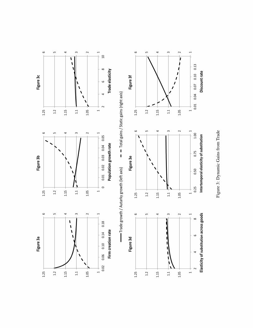
Trad
e g
row
th /
Au
tark
y gr
ow
th (
left
axi
s)To
tal g
ain
s /
Stat
ic g
ain
s (r
igh
t ax
is)
123456
1
1.0
5
1.1
1.1
5
1.2
1.2
5
0.0
20
.06
0.1
00
.14
0.1
8
Firm
cre
ati
on
ra
te
Figu
re 3
a
123456
1
1.0
5
1.1
1.1
5
1.2
1.2
5
00
.01
0.0
20
.03
0.0
40
.05
Po
pu
lati
on
gro
wth
ra
te
Figu
re 3
b
123456
1
1.0
5
1.1
1.1
5
1.2
1.2
5
24
68
10
Tra
de
ela
stic
ity
Figu
re 3
c
123456
1
1.0
5
1.1
1.1
5
1.2
1.2
5
24
68
Ela
stic
ity
of
sub
stit
uti
on
acr
oss
go
od
s
Figu
re 3
d
123456
1
1.0
5
1.1
1.1
5
1.2
1.2
5
0.2
50
.50
0.7
51
.00
Inte
rte
mp
ora
l ela
stic
ity
of
sub
stit
uti
on
Figu
re 3
e
123456
1
1.0
5
1.1
1.1
5
1.2
1.2
5
0.0
10
.04
0.0
70
.10
0.1
3
Dis
cou
nt
rate
Figu
re 3
f
Figu
re3:
Dyn
amic
Gai
nsfr
omTr
ade
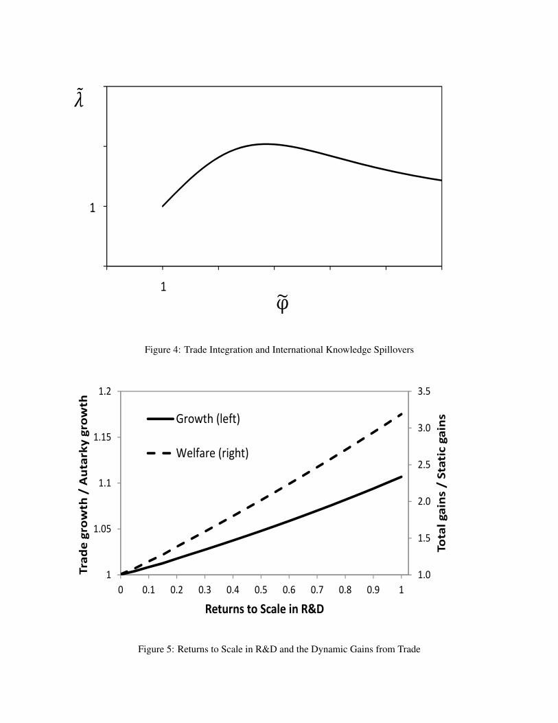
0
1
2
3
0 1 2 3 4 5 6
Ax
is T
itle
φ
1
1
φ�
��
Figure 4: Trade Integration and International Knowledge Spillovers
1.0
1.5
2.0
2.5
3.0
3.5
1
1.05
1.1
1.15
1.2
0 0.1 0.2 0.3 0.4 0.5 0.6 0.7 0.8 0.9 1
To
tal
ga
ins /
Sta
tic g
ain
s
Tra
de
gro
wth
/ A
uta
rky
gro
wth
Returns to Scale in R&D
Growth (left)
Welfare (right)
Figure 5: Returns to Scale in R&D and the Dynamic Gains from Trade