dynamic shape reconstruction of three-dimensional frame
TRANSCRIPT

December 2011
NASA/TP–2011-217315
Dynamic Shape Reconstruction of Three-Dimensional Frame Structures Using the Inverse Finite Element Method Marco Gherlone, Priscilla Cerracchio, Massimiliano Mattone, and Marco Di Sciuva Department of Aeronautics and Space Engineering Politecnico di Torino, Torino, Italy Alexander Tessler Langley Research Center, Hampton, Virginia

NASA STI Program . . . in Profile
Since its founding, NASA has been dedicated to the advancement of aeronautics and space science. The NASA scientific and technical information (STI) program plays a key part in helping NASA maintain this important role.
The NASA STI program operates under the auspices of the Agency Chief Information Officer. It collects, organizes, provides for archiving, and disseminates NASA’s STI. The NASA STI program provides access to the NASA Aeronautics and Space Database and its public interface, the NASA Technical Report Server, thus providing one of the largest collections of aeronautical and space science STI in the world. Results are published in both non-NASA channels and by NASA in the NASA STI Report Series, which includes the following report types:
TECHNICAL PUBLICATION. Reports of
completed research or a major significant phase of research that present the results of NASA programs and include extensive data or theoretical analysis. Includes compilations of significant scientific and technical data and information deemed to be of continuing reference value. NASA counterpart of peer-reviewed formal professional papers, but having less stringent limitations on manuscript length and extent of graphic presentations.
TECHNICAL MEMORANDUM. Scientific
and technical findings that are preliminary or of specialized interest, e.g., quick release reports, working papers, and bibliographies that contain minimal annotation. Does not contain extensive analysis.
CONTRACTOR REPORT. Scientific and
technical findings by NASA-sponsored contractors and grantees.
CONFERENCE PUBLICATION. Collected
papers from scientific and technical conferences, symposia, seminars, or other meetings sponsored or co-sponsored by NASA.
SPECIAL PUBLICATION. Scientific,
technical, or historical information from NASA programs, projects, and missions, often concerned with subjects having substantial public interest.
TECHNICAL TRANSLATION. English-
language translations of foreign scientific and technical material pertinent to NASA’s mission.
Specialized services also include creating custom thesauri, building customized databases, and organizing and publishing research results. For more information about the NASA STI program, see the following: Access the NASA STI program home page at
http://www.sti.nasa.gov E-mail your question via the Internet to
[email protected] Fax your question to the NASA STI Help Desk
at 443-757-5803 Phone the NASA STI Help Desk at
443-757-5802 Write to:
NASA STI Help Desk NASA Center for AeroSpace Information 7115 Standard Drive Hanover, MD 21076-1320
National Aeronautics and Space Administration Langley Research Center Hampton, Virginia 23681-2199
December 2011
NASA/TP–2011-217315
Dynamic Shape Reconstruction of Three-Dimensional Frame Structures Using the Inverse Finite Element Method Marco Gherlone, Priscilla Cerracchio, Massimiliano Mattone, and Marco Di Sciuva Department of Aeronautics and Space Engineering Politecnico di Torino, Torino, Italy Alexander Tessler Langley Research Center, Hampton, Virginia

Available from:
NASA Center for AeroSpace Information 7115 Standard Drive
Hanover, MD 21076-1320 443-757-5802
The use of trademarks or names of manufacturers in this report is for accurate reporting and does not constitute an official endorsement, either expressed or implied, of such products or manufacturers by the National Aeronautics and Space Administration.
1
Abstract
A robust and efficient computational method for reconstructing the
three-dimensional displacement field of truss, beam, and frame
structures, using measured surface-strain data, is presented. Known as
“shape sensing”, this inverse problem has important implications for
real-time actuation and control of smart structures, and for monitoring
of structural integrity. The present formulation, based on the inverse
Finite Element Method (iFEM), uses a least-squares variational
principle involving strain measures of Timoshenko theory for stretching,
torsion, bending, and transverse shear. Two inverse-frame finite
elements are derived using interdependent interpolations whose interior
degrees-of-freedom are condensed out at the element level. In addition,
relationships between the order of kinematic-element interpolations and
the number of required strain gauges are established. As an example
problem, a thin-walled, circular cross-section cantilevered beam
subjected to harmonic excitations in the presence of structural damping
is modeled using iFEM; where, to simulate strain-gauge values and to
provide reference displacements, a high-fidelity MSC/NASTRAN shell
finite element model is used. Examples of low and high-frequency
dynamic motion are analyzed and the solution accuracy examined with
respect to various levels of discretization and the number of strain
gauges.
Nomenclature
, ,x y z Cartesian coordinate system
, ,x r cylindrical coordinate system
1 2 3, ,x x x
local “strain-gauge” coordinate system
E, G, , Young’s modulus, shear modulus, Poisson ratio, and density
L, A length and cross-sectional area of frame member
yI , zI area moments of inertia with respect to the y - and z -axis
PI polar moment of inertia
xu , yu ,
zu displacements along x -, y -, and z -axis
2
u , v , w displacements along along x -, y -, and z -axis
x, y, z rotations about x -, y -, and z -axis
, , , , ,T
x y zu v w u vector of the kinematic variables
hu vector of the approximated kinematic variables
x , xz , xy non vanishing components of the strain tensor for the Timoshenko
beam theory in the (x,y,z) coordinate system
x , , x components of the strain tensor for the Timoshenko beam theory
in the , x plane
*
2 strain measured by the strain-gauge
x , , x components of the stress tensor for the Timoshenko beam theory
in the , x plane
( 1,...,6)ie i section strains
1 2 3 4 5 6, , , , ,T
e e e e e ee vector of the section strains
e experimentally evaluated section strains
N, Qy, Qz, Mx, My, Mz section forces and moments
Ax, Gy, Gz, Jx, Dy, Dz axial rigidity, shear rigidities, torsional rigidity and bending
rigidities of the beam
2
yk , 2
zk shear correction factors
qx, qy, qz distributed loads along the x-, y-, and z-direction
least-squares functional
eu vector of the nodal degrees of freedom of the inverse finite
element
N matrix of the shape functions relating the kinematic variables to
the nodal degrees of freedom
B matrix of the shape functions relating the section strains to the
nodal degrees of freedom
0 , ( 1,...,6)k kw w k weighting coefficients
,e eL A , e
yI , e
zI , e
PI length, cross-sectional area and moments of inertia of frame
inverse element
n , ix number and axial coordinate of the locations where the section
strains are evaluated
3
,e ek f matrix and vector of the single inverse element governing equation
,Κ F matrix and vector of the whole structure governing equation
(1)
iL linear Lagrange polynomials
(2)
jL quadratic Lagrange polynomials
(3)(3) , kjN N special cubic polynomials
(4)
kL quartic Lagrange polynomials
orientation of a strain-gauge with respect to the beam axis
extR external radius of the circular cross-sectio
R, t radius and thickness of the thin-walled circular cross section
Fz(t) time varying applied force
Fz0 amplitude of the applied force
f0 frequency of the applied force
4
1 Introduction
Real-time reconstruction of structural deformations using measured strain data, is a key technology for
actuation and control of smart structures, as well as for Structural Health Monitoring (SHM) [1]. Known
as “shape sensing”, this inverse problem is commonly formulated with the assumption that multiple strain
sensors at various structural locations provide real-time strain measurements. Most inverse algorithms use
some type of Tikhonov’s regularization, which is manifested by constraint (regularity) terms that ensure a
certain degree of solution smoothness (refer to [2-5] and references therein).
Most of the shape sensing efforts focused exclusively on beam-bending problems. Davis et al. [6] used
optimized trial functions and weights to reconstruct a simple static-beam response from discrete strain
measurements. To model more complex deformations, the approach requires a large number of trial
functions and strain sensors. Kang et al. [7] used vibration mode shapes to reconstruct a beam response
due to dynamic excitation. In their approach, modal coordinates are computed using strain-displacement
relationships and measured surface strains; the method requires the same number of mode shapes and
strain sensors. Kim et al. [8] and Ko et al. [9] used classical beam equations to integrate discretely
measured strains to determine the deflection of a beam. By regression of experimental strain data and by
accounting for the applied loading, Kim et al. [8] obtained a continuous curvature function, leading to the
evaluation of beam deflection. Ko et al. [9] developed a load-independent method by approximating the
beam curvature using piece-wise continuous polynomials; the authors demonstrated the validity of a one-
dimensional scheme by evaluating the deflection and cross-section twist of an aircraft wing.
To enable shape-sensing analyses of plates undergoing bending deformations, Bogert et al. [10]
examined a modal transformation method that allows the development of suitable strain-displacement
transformations. The approach makes use of a large number of natural vibration modes. When applied to
high-fidelity finite element models, however, the method requires a computationally intensive eigenvalue
analysis and a detailed description of the elastic and inertial material properties. Jones et al. [11]
employed a least-squares formulation for shape sensing of a cantilever plate, where the axial strain was
fitted with a cubic polynomial. The strain field was then integrated with the use of approximate boundary
conditions at the clamped end to obtain plate deflections according to classical bending assumptions.
Shkarayev et al. [12,13] used a two-step solution procedure: the first step involves the structural analysis
of a plate/shell finite element model, and the second, a least-squares algorithm. The methodology
reconstructs the applied loading first, which then leads to the displacements. In a series of four papers,
Mainçon and co-authors [14-17] developed a finite element formulation that seeks the solution for the
displacements and loads simultaneously, requiring a priori knowledge of a subset of applied loading and
the material properties. The solution procedure minimizes a cost function consisting of unknown loads
and differences between the measured and estimated quantities (displacements or strains); the cost
function is regularized by way of equilibrium constraints. The number of unknowns is three times the
number of the degrees-of-freedom in the finite element discretization. Importantly, the accuracy of the
solution strongly depends on the choice of suitable weights; these are computed from a complex
procedure involving the probability distributions of the unknown loads and measured data. In [16,17],
sensitivity analyses were carried out for truss structures, investigating variations in the input data as well
as the modeling errors. Nishio et al. [18] employed a weighted-least-squares formulation to reconstruct,
on the basis of measured strain data, the deflection of a composite cantilevered plate. The weighting
coefficients in the least-square terms were adjusted in order to account for the inherent errors in the
measured strain data. The weights were computed for a given data-acquisition apparatus, load case, and
test article, with the consequent difficulties in generalizing the procedure.
Many of the aforementioned inverse methods either lack generality with respect to structural topology
and boundary conditions, or require sufficiently accurate loading and/or elastic-inertial material
information – the kind of data that are either unavailable or difficult to obtain outside the laboratory
environment; for these reasons, such approaches are generally unsuited for use in onboard SHM
5
algorithms. A well-suited algorithm for SHM should be: (1) general enough to accommodate complex
structural topologies and boundary conditions (e.g., built-up aircraft structures), (2) robust, stable, and
accurate under a wide range of loadings, material systems, inertial/damping characteristics, and inherent
errors in the strain measurements, and (3) sufficiently fast for real-time applications.
An algorithm that appears to fulfill the aforementioned requirements was recently developed by
Tessler and Spangler [1,19]. The methodology, labeled the inverse Finite Element Method (iFEM),
employs a weighted-least-square variational principle which is discretized by C0-continuous finite
elements that accommodate arbitrarily positioned and oriented strain-sensor data. The iFEM framework,
providing accurate and stable solutions of the displacement and strain fields for a discretized structural
domain, is amenable to any type of structural modeling including frame (truss and beam), plate, shell, and
solid idealizations. Because only strain-displacement relations are used in the formulation, both static and
dynamic response can be reconstructed without any a priori knowledge of material, inertial, loading, or
damping structural properties. To model arbitrary plate and shell structures, Tessler [20] developed, using
first-order shear-deformation theory, a three-node inverse shell element. Numerically generated [20] and
experimentally measured-strain data [21,22] were used to assess robustness and accuracy of the
formulation.
The present paper consolidates the authors’ recent efforts [23-24] and presents the development and
assessment of simple and efficient inverse-frame finite elements. The methodology permits effective and
computationally efficient shape-sensing analyses to be performed on truss, beam, and frame structures
instrumented with strain gauges. The kinematic assumptions are those of Timoshenko shear-deformation
theory [25]; they incorporate stretching, torsion, bending, and transverse shear deformation modes in
three dimensions. The formulation uses a least-squares variational principle that is specialized from [19]
for three-dimensional frame analysis. The variational framework, in conjunction with suitable finite
element discretizations involving inverse finite elements, yields a system of linear algebraic equations; the
equations are efficiently solved for the unknown displacement degrees-of-freedom (dof’s), thus providing
the deformed structural-shape predictions.
In the remainder of the paper, the kinematic assumptions for a three-dimensional frame are discussed,
followed by the description of the least-squares variational principle suitable for three-dimensional
deformations of frame structures. This is followed by a discussion of two C0-continuous, inverse-frame
elements that use the well-established interdependent interpolations that resolve the shear locking effect.
Finally, to examine the predictive capabilities of the inverse elements for a given set of distributed strain
gauges, shape-sensing studies are carried out for a cantilevered beam undergoing harmonic excitations in
the presence of structural damping.
2 Governing equations
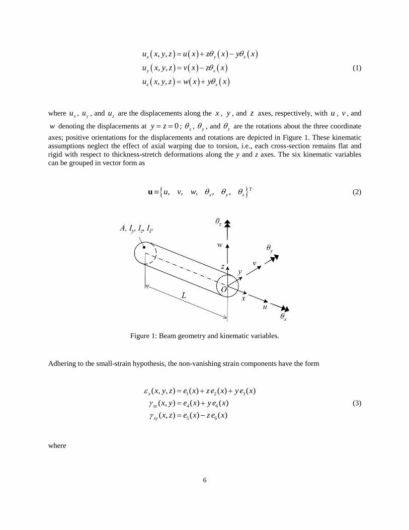
Consider a straight frame member of constant cross-section referred to the three-dimensional
Cartesian coordinates (x,y,z) as depicted in Figure 1; the coordinate origin, O, is located at the cross-
section’s center of mass, which is also coincident with the shear center. The longitudinal, elastic x-axis is
normal to the cross-sectional plane (y, z), where y and z are the cross-section’s principal inertial axes. The
frame member has length L and its cross-section has area A, area moments of inertia with respect to the
y - and z -axis yI and zI , respectively, and polar moment of inertia P y zI I I (Figure 1). The frame
member is made of an isotropic homogeneous material, represented by the elastic constants: E (Young’s
modulus), G (shear modulus), and v (Poisson ratio).
The three Cartesian components of the displacement vector that are consistent with the kinematic
assumptions of Timoshenko theory [25] for three-dimensional deformations are given by
6
, ,
, ,
, ,
x y z
y x
z x
u x y z u x z x y x
u x y z v x z x
u x y z w x y x
(1)
where xu , yu , and zu are the displacements along the x , y , and z axes, respectively, with u , v , and
w denoting the displacements at 0y z ; x , y , and z are the rotations about the three coordinate
axes; positive orientations for the displacements and rotations are depicted in Figure 1. These kinematic
assumptions neglect the effect of axial warping due to torsion, i.e., each cross-section remains flat and
rigid with respect to thickness-stretch deformations along the y and z axes. The six kinematic variables
can be grouped in vector form as
, , , , , T
x y zu v w u (2)
Figure 1: Beam geometry and kinematic variables.
Adhering to the small-strain hypothesis, the non-vanishing strain components have the form
1 2 3
4 6
5 6
( , , ) ( ) ( ) ( )
( , ) ( ) ( )
( , ) ( ) ( )
x
xz
xy
x y z e x z e x y e x
x y e x y e x
x z e x z e x
(3)
where
7
1 2 3 4 5 6( ) , , , , ,T
e e e e e ee u (4)
denote the section strains of the theory, given by
1 , 4 ,
2 , 5 ,
3 , 6 ,
( ) ( ) ( ) ( ) ( )
( ) ( ) ( ) ( ) ( )
( ) ( ) ( ) ( )
x x y
y x x z
z x x x
e x u x e x w x x
e x x e x v x x
e x x e x x
(5)
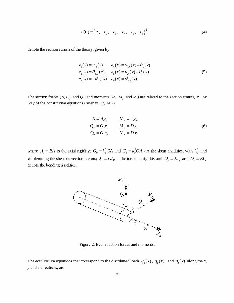
The section forces (N, Qy, and Qz) and moments (Mx, My, and Mz) are related to the section strains, ie , by
way of the constitutive equations (refer to Figure 2)
1 6
5 2
4 3
N M
Q M
Q M
x x x
y y y y
z z z z
A e J e
G e D e
G e D e
(6)
where xA EA is the axial rigidity; 2
y yG k GA and 2
z zG k GA are the shear rigidities, with 2
yk and
2
zk denoting the shear correction factors; x PJ GI is the torsional rigidity and y yD EI and z zD EI
denote the bending rigidities.
Figure 2: Beam section forces and moments.
The equilibrium equations that correspond to the distributed loads ( )xq x , ( )yq x , and ( )zq x along the x,
y and z directions, are
8
dMdN0
d d
dQ dMQ
d d
dQ dMQ
d d
xx
y y
y z
z zz y
qx x
qx x
qx x
(7)
To reconstruct the deformed shape of a frame-member for which certain in-situ strain measurements
are known, a functional ( ) u that matches in a least-squares sense the complete set of analytic section
strains,
( )e u , to the in-situ section strains,
εe , is minimized with respect to the kinematic variables, u ;
( ) u functional can be written as
2 u e u e (8)
This functional may be used in a finite element framework by introducing a discretization in which the
element kinematic field is interpolated by C0-continuous shape functions,
( )h ex xu u N u (9)
where ( )xN denotes the shape functions and eu nodal dof’s. Thus, the total least-squares functional is a
sum of the individual element contributions, ( )e h u , i.e., 1
Ne
e
, with N denoting the total number
of elements. Accounting for the axial stretching, bending, twisting, and transverse shearing, the element
functional is given by the dot product of the weighting coefficient vector,
0 0 0 0 0 0
1 2 3 4 5 6, , , , ,e e e e e e
k y z Pw w w I A w I A w w w I A w , and the least-squares
component vector, e
k Φ ,
( )e h u w Φ (10)
where 0 ( 1,...,6)kw k denote dimensionless weighting coefficients;
eA , e
yI , e
zI , and e
PI are,
respectively, the cross-section area, moments of inertia with respect to the y - and z -axis, and polar
moment of inertia of the element, and
9
2
1
( 1,...,6)e n
e i
k k i k
i
Le x e k
n
(11)
denote the least-squares components of the element functional, where eL denotes the element length; n
and ix ( 0 e
ix L ) are, respectively, the number and the axial coordinate of the locations where the
section strains are evaluated, and the superscript i is used to denote the section strains that are computed
from the strain-sensor values (experimental values) at the location ix . The 0
kw coefficients may be
assigned different values to enforce a stronger or weaker correlation between the measured section-strain
components and their analytic counterparts, i.e., a larger value of 0
kw enforces a stronger correlation,
whereas a smaller value enforces a weaker correlation.
Substituting Eq. (9) into Eq. (3) gives the section strains in terms of the nodal dof’s as
( 1,...,6)e
k ke k B u (12)
A vector form of Eq. (12) that incorporates all six section strains is given by
exe u B u (13)
where the matrix xB contains the derivatives of the shape functions ( )xN ( xB is defined in
Appendix B for the case of shape functions presented in Sec. 3.) Substituting Eq. (13) into Eq. (11) and
then Eq. (10) results in the following quadratic form
1
2
T Te e e e e e e u k u u f c (14)
where e
c is a constant while e
k and e
f are defined as follows
6 6
1 1
,k k k k
k k
w w
e e e ek k f f (15)
with
10
1 1
, ( 1,...,6)e en n
T T i
k k i k i k k i k
i i
L Lx x x e k
n n
e ek B B f B (16)
Note that e
k resembles an element stiffness matrix of the direct finite element method and e
f resembles
the load vector; e
k is a function of the measurement locations, ix , whereas
ef possesses the measured
strain values. Minimization of functional e (see Eq. (14)) with respect to
eu leads to the inverse
element matrix equation
e e ek u f (17)
The assembly of the finite element contributions, while accounting for the appropriate coordinate
transformations and by specifying problem-dependent displacement boundary conditions, results in a non
singular system of algebraic equations of the form
ΚU F (18)
The solution of these equations for the unknown dof’s is efficient: the K matrix is inverted only once,
since it is independent of the values of the measured strains. The F vector, however, is dependent on the
measured strain values that change during deformation. Thus, at any strain-measurement update during
deformation, the matrix-vector multiplication provides the solution for the unknown nodal displacement
dof’s, U = K-1
F, where K-1
remains unchanged for a given distribution of strain sensors.
The remaining part of the element formulation involves the selection of suitable shape functions,
symbolically defined by Eq. (9), and the computation of the experimental section strains, i
ke, appearing
in Eqs. (12),(13). In Sec. 3, the shape functions for two alternative inverse-frame elements, each having
two nodes and twelve dof’s, are derived. In Sec. 4, a procedure for computing i
ke is described; it relates
the number of strain gauges to the interpolation order of the shape functions.
3 Element shape functions
In this section, inverse frame elements of 0th- and 1
st-order are formulated. The elements use C
0-
continuous interdependent interpolations that enable excellent predictions even for very slender frame
members, without incurring any form of excessive stiffening due to shear locking [26]. The 0th-order
shape functions are guided by Timoshenko equilibrium equations, Eqs. (7), that correspond to the forces
and moments applied exclusively at the end nodes, resulting in constant distributions of the transverse-
shear section strains. The 1st-order shape functions accommodate Eqs. (7) for uniformly distributed
transverse loads, giving rise to linear distributions of the transverse-shear section strains.
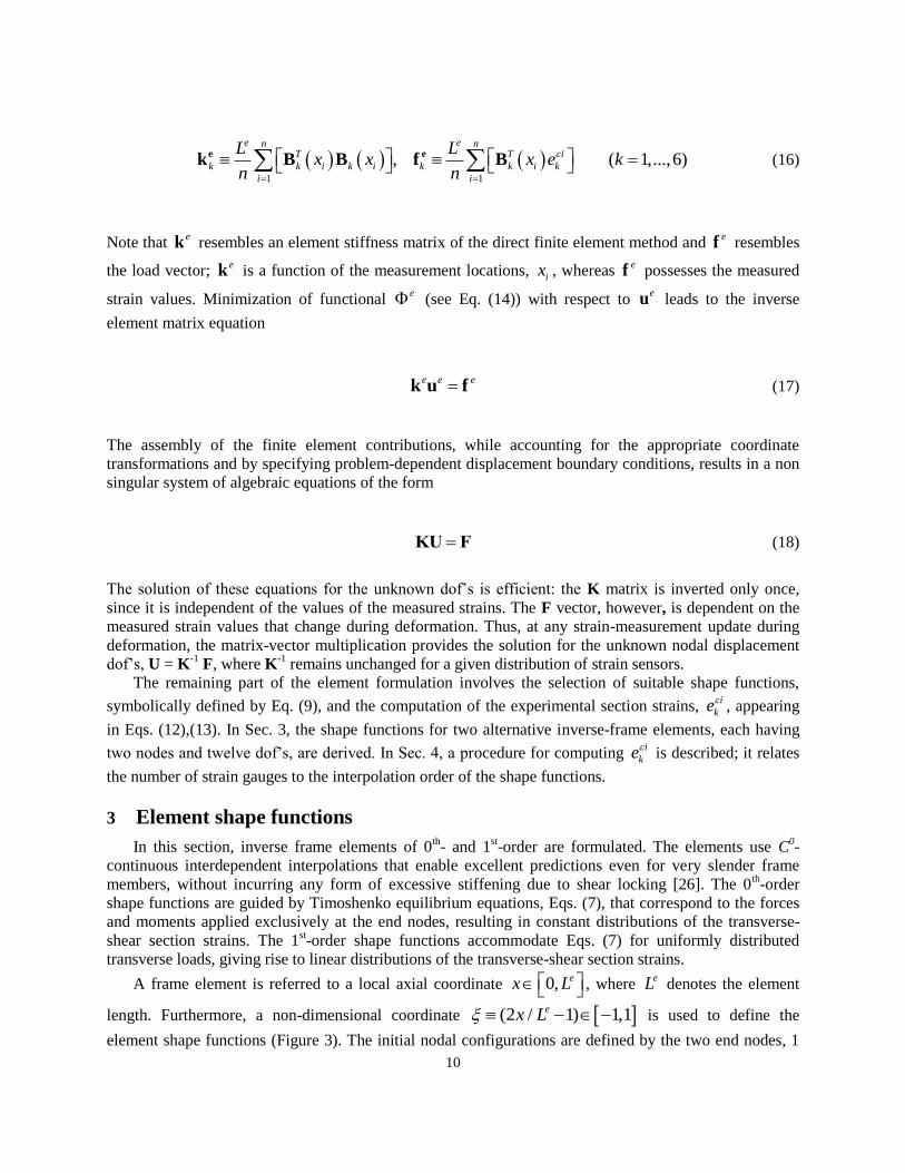
A frame element is referred to a local axial coordinate 0, ex L , where eL denotes the element
length. Furthermore, a non-dimensional coordinate (2 / 1) 1,1ex L is used to define the
element shape functions (Figure 3). The initial nodal configurations are defined by the two end nodes, 1
11
(at 1 ) and 2 (at 1 ) and one or three interior nodes. Thus, the initial configuration for the 0th-
order element has the interior node, r (at the midspan, 0 ); whereas the interior nodes of the 1st-order
element are q (at 1 2 ), r (at 0 ), and s (at 1 2 ) .
Figure 3: Inverse finite element geometry and nodal topology.
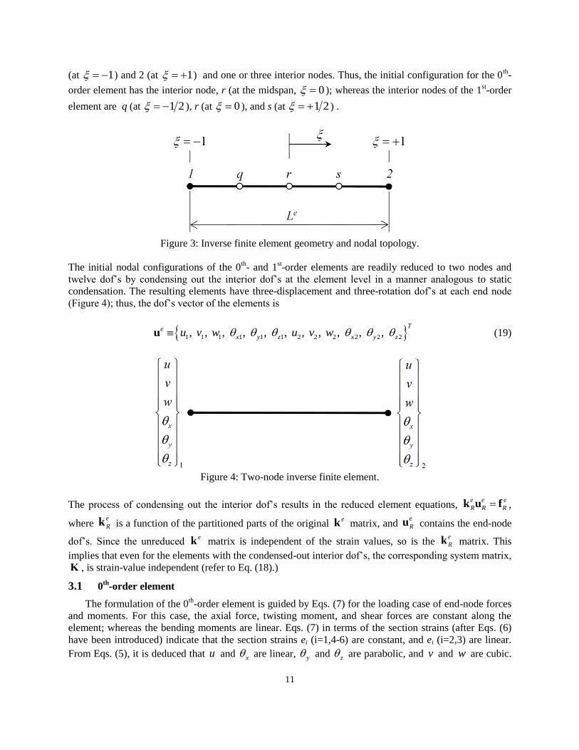
The initial nodal configurations of the 0th- and 1
st-order elements are readily reduced to two nodes and
twelve dof’s by condensing out the interior dof’s at the element level in a manner analogous to static
condensation. The resulting elements have three-displacement and three-rotation dof’s at each end node
(Figure 4); thus, the dof’s vector of the elements is
1 1 1 1 1 1 2 2 2 2 2 2, , , , , , , , , , , T
e
x y z x y zu v w u v w u (19)
Figure 4: Two-node inverse finite element.
The process of condensing out the interior dof’s results in the reduced element equations, e e e
R R Rk u f ,
where e
Rk is a function of the partitioned parts of the original e
k matrix, and e
Ru contains the end-node
dof’s. Since the unreduced e
k matrix is independent of the strain values, so is the e
Rk matrix. This
implies that even for the elements with the condensed-out interior dof’s, the corresponding system matrix, Κ , is strain-value independent (refer to Eq. (18).)
3.1 0th
-order element
The formulation of the 0th-order element is guided by Eqs. (7) for the loading case of end-node forces
and moments. For this case, the axial force, twisting moment, and shear forces are constant along the
element; whereas the bending moments are linear. Eqs. (7) in terms of the section strains (after Eqs. (6)
have been introduced) indicate that the section strains ei (i=1,4-6) are constant, and ei (i=2,3) are linear.
From Eqs. (5), it is deduced that u and x are linear, y and z are parabolic, and v and w are cubic.
12
The inter-relationship of the polynomial order of the deflection variables, v and w , and bending
rotations, y and z , can also be inferred from the definitions of the transverse shear section strains [24]
4 , 5 ,,x y x ze w e v (20)
It is understood that in 4e both ,xw and y should be represented by the same polynomial order and,
similarly, in 5e both ,xv and z should also have matching polynomial orders. The above interpolations
give rise to quadratic interpolations for 4e and 5e ; they permit a consistent reduction of interior dof’s for
v and w by requiring a constant variation of these section strains across the element span
4 5., .e const e const (21)
The complete set of interpolations for this element is thus given by
(1) (1)
1,2 1,2
(2) (2)
1, ,2 1, ,2
(1) (3) (1) (3)
1,2 1, ,2 1,2 1, ,2
,
,
,
i i x i xi
i i
y j yj z j zj
j r j r
i i j zj i i j yj
i j r i j r
u L u L
L L
v L v N w L w N
(22)
where (1)
iL 1,2i and (2)
jL 1, ,2j r are, respectively, linear and quadratic Lagrange
polynomials, and (3)
jN 1, ,2j r are special-form cubic polynomials (refer to Appendix A.) Static
condensation can be used to condense out the two interior dof’s ( yr and zr , refer to Eqs. (22)), thus,
achieving a two-node element with twelve dof’s (Figure 4, Eq. (19)).
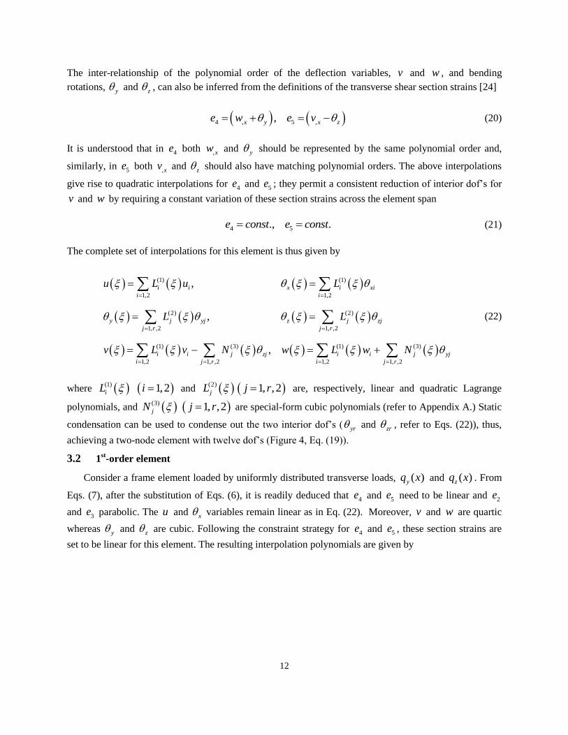
3.2 1st-order element
Consider a frame element loaded by uniformly distributed transverse loads, ( )yq x and ( )zq x . From
Eqs. (7), after the substitution of Eqs. (6), it is readily deduced that 4e and 5e need to be linear and 2e
and 3e parabolic. The u and x variables remain linear as in Eq. (22). Moreover, v and w are quartic
whereas y and z are cubic. Following the constraint strategy for 4e and 5e , these section strains are
set to be linear for this element. The resulting interpolation polynomials are given by
13
(1) (1)
1,2 1,2
(4) (4)
1, , , ,2 1, , , ,2
(3) (3)(1) (1)
1,2 1, , , ,2 1,2 1, , , ,2
,
,
,
i i x i xi
i i
k k k k
k q r s k q r s
k ky i yi k z i zi k
i k q r s i k q r s
u L u L
v L v w L w
L N w L N v
(23)
where (3)
kN 1, , , ,2k q r s are cubic polynomials that satisfy the conditions
4 5,e linear e linear (24)
For the detailed expressions of the (3)
kN polynomials, refer to Appendix A. The interior dof’s ( qv ,
rv , sv , qw , rw , and sw , refer to Eqs. (23)) are condensed out at the element level, leading again to a
twelve dof’s inverse element as in Eq. (19).
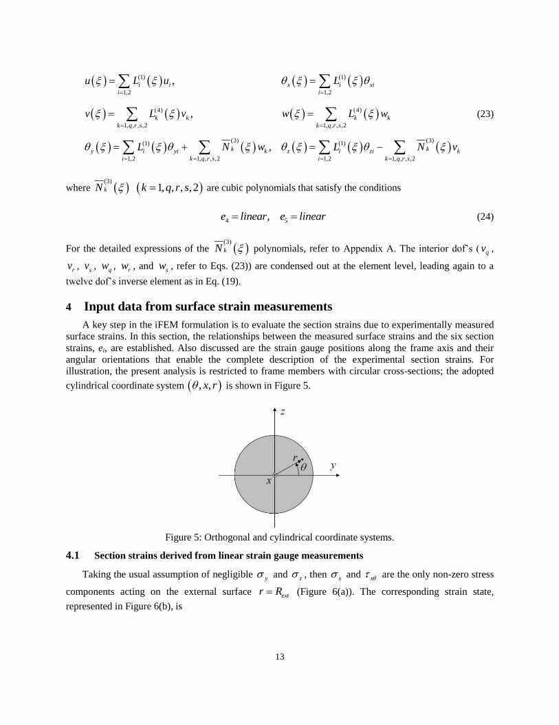
4 Input data from surface strain measurements
A key step in the iFEM formulation is to evaluate the section strains due to experimentally measured
surface strains. In this section, the relationships between the measured surface strains and the six section
strains, ei, are established. Also discussed are the strain gauge positions along the frame axis and their
angular orientations that enable the complete description of the experimental section strains. For
illustration, the present analysis is restricted to frame members with circular cross-sections; the adopted
cylindrical coordinate system , ,x r is shown in Figure 5.
Figure 5: Orthogonal and cylindrical coordinate systems.
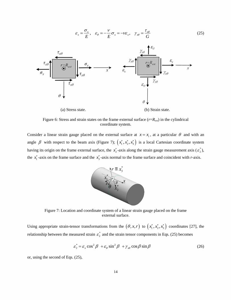
4.1 Section strains derived from linear strain gauge measurements
Taking the usual assumption of negligible y and z , then x and x are the only non-zero stress
components acting on the external surface extr R (Figure 6(a)). The corresponding strain state,
represented in Figure 6(b), is
14
, ,x xx x x x
E E G
(25)
(a) Stress state. (b) Strain state.
Figure 6: Stress and strain states on the frame external surface (r=Rext) in the cylindrical
coordinate system.
Consider a linear strain gauge placed on the external surface at ix x , at a particular and with an
angle with respect to the beam axis (Figure 7); 1 2 3, ,x x x is a local Cartesian coordinate system
having its origin on the frame external surface, the 2x-axis along the strain gauge measurement axis (
*
2 ),
the 1x-axis on the frame surface and the 3x
-axis normal to the frame surface and coincident with r-axis.
Figure 7: Location and coordinate system of a linear strain gauge placed on the frame
external surface.
Using appropriate strain-tensor transformations from the , ,x r to 1 2 3, ,x x x coordinates [27], the
relationship between the measured strain *
2 and the strain tensor components in Eqs. (25) becomes
* 2 2
2 cos sin cos sin x x (26)
or, using the second of Eqs. (25),
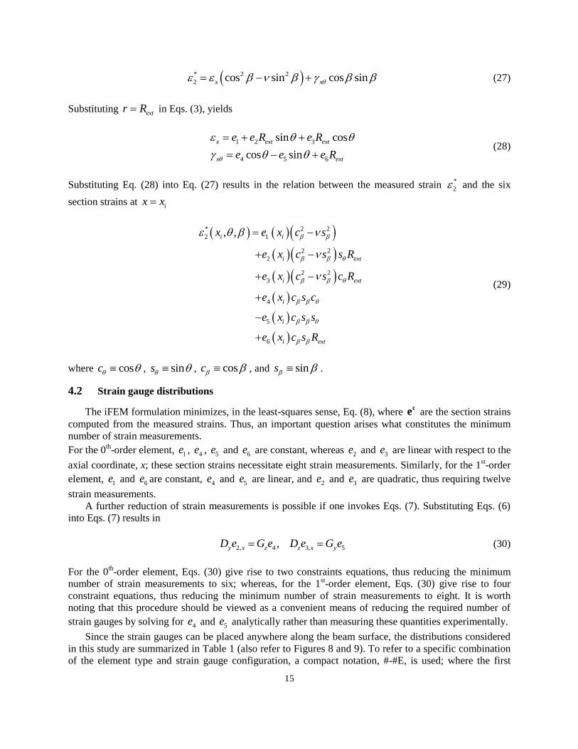
15
* 2 2
2 cos sin cos sinx x (27)
Substituting extr R in Eqs. (3), yields
1 2 3
4 5 6
sin cos
cos sin
x ext ext
x ext
e e R e R
e e e R
(28)
Substituting Eq. (28) into Eq. (27) results in the relation between the measured strain *
2 and the six
section strains at ix x
* 2 2
2 1
2 2
2
2 2
3
4
5
6
, ,
i i
i ext
i ext
i
i
i ext
x e x c s
e x c s s R
e x c s c R
e x c s c
e x c s s
e x c s R
(29)
where cosc , sins , cosc , and sins .
4.2 Strain gauge distributions
The iFEM formulation minimizes, in the least-squares sense, Eq. (8), where εe are the section strains
computed from the measured strains. Thus, an important question arises what constitutes the minimum
number of strain measurements.
For the 0th-order element, 1e , 4e , 5e and 6e are constant, whereas 2e and 3e are linear with respect to the
axial coordinate, x; these section strains necessitate eight strain measurements. Similarly, for the 1st-order
element, 1e and 6e are constant, 4e and 5e are linear, and 2e and 3e are quadratic, thus requiring twelve
strain measurements.
A further reduction of strain measurements is possible if one invokes Eqs. (7). Substituting Eqs. (6)
into Eqs. (7) results in
2, 4 3, 5,y x z z x yD e G e D e G e (30)
For the 0th-order element, Eqs. (30) give rise to two constraints equations, thus reducing the minimum
number of strain measurements to six; whereas, for the 1st-order element, Eqs. (30) give rise to four
constraint equations, thus reducing the minimum number of strain measurements to eight. It is worth
noting that this procedure should be viewed as a convenient means of reducing the required number of
strain gauges by solving for 4e and 5e analytically rather than measuring these quantities experimentally.
Since the strain gauges can be placed anywhere along the beam surface, the distributions considered
in this study are summarized in Table 1 (also refer to Figures 8 and 9). To refer to a specific combination
of the element type and strain gauge configuration, a compact notation, #-#E, is used; where the first
16
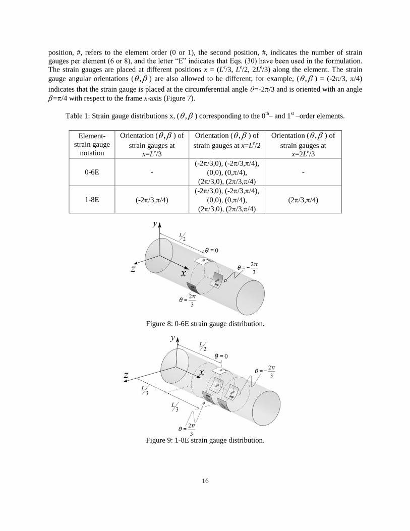
position, #, refers to the element order (0 or 1), the second position, #, indicates the number of strain
gauges per element (6 or 8), and the letter “E” indicates that Eqs. (30) have been used in the formulation.
The strain gauges are placed at different positions x = (Le/3, L
e/2, 2L
e/3) along the element. The strain
gauge angular orientations ( , ) are also allowed to be different; for example, ( , ) = (-2/3, /4)
indicates that the strain gauge is placed at the circumferential angle =-2/3 and is oriented with an angle
=/4 with respect to the frame x-axis (Figure 7).
Table 1: Strain gauge distributions x, ( , ) corresponding to the 0th– and 1
st –order elements.
Element-
strain gauge
notation
Orientation ( , ) of
strain gauges at
x=Le/3
Orientation ( , ) of
strain gauges at x=Le/2
Orientation ( , ) of
strain gauges at
x=2Le/3
0-6E -
(-2/3,0), (-2/3,/4),
(0,0), (0,/4),
(2/3,0), (2/3,/4)
-
1-8E (-2/3,/4)
(-2/3,0), (-2/3,/4),
(0,0), (0,/4),
(2/3,0), (2/3,/4)
(2/3,/4)
Figure 8: 0-6E strain gauge distribution.
Figure 9: 1-8E strain gauge distribution.
17
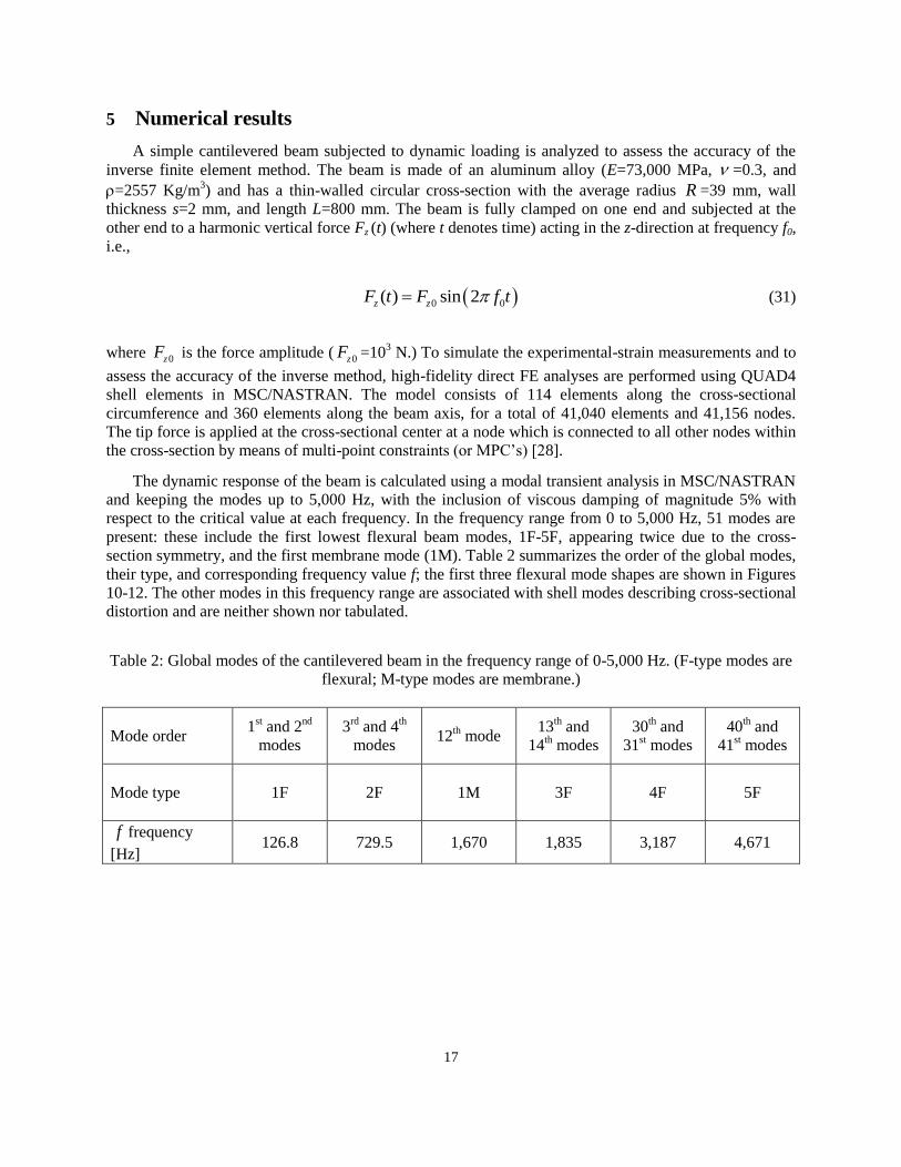
5 Numerical results
A simple cantilevered beam subjected to dynamic loading is analyzed to assess the accuracy of the
inverse finite element method. The beam is made of an aluminum alloy (E=73,000 MPa, =0.3, and
=2557 Kg/m3) and has a thin-walled circular cross-section with the average radius R =39 mm, wall
thickness s=2 mm, and length L=800 mm. The beam is fully clamped on one end and subjected at the
other end to a harmonic vertical force Fz (t) (where t denotes time) acting in the z-direction at frequency f0,
i.e.,
0 0( ) sin 2z zF t F f t (31)
where 0zF is the force amplitude ( 0zF =103 N.) To simulate the experimental-strain measurements and to
assess the accuracy of the inverse method, high-fidelity direct FE analyses are performed using QUAD4
shell elements in MSC/NASTRAN. The model consists of 114 elements along the cross-sectional
circumference and 360 elements along the beam axis, for a total of 41,040 elements and 41,156 nodes.
The tip force is applied at the cross-sectional center at a node which is connected to all other nodes within
the cross-section by means of multi-point constraints (or MPC’s) [28].
The dynamic response of the beam is calculated using a modal transient analysis in MSC/NASTRAN
and keeping the modes up to 5,000 Hz, with the inclusion of viscous damping of magnitude 5% with
respect to the critical value at each frequency. In the frequency range from 0 to 5,000 Hz, 51 modes are
present: these include the first lowest flexural beam modes, 1F-5F, appearing twice due to the cross-
section symmetry, and the first membrane mode (1M). Table 2 summarizes the order of the global modes,
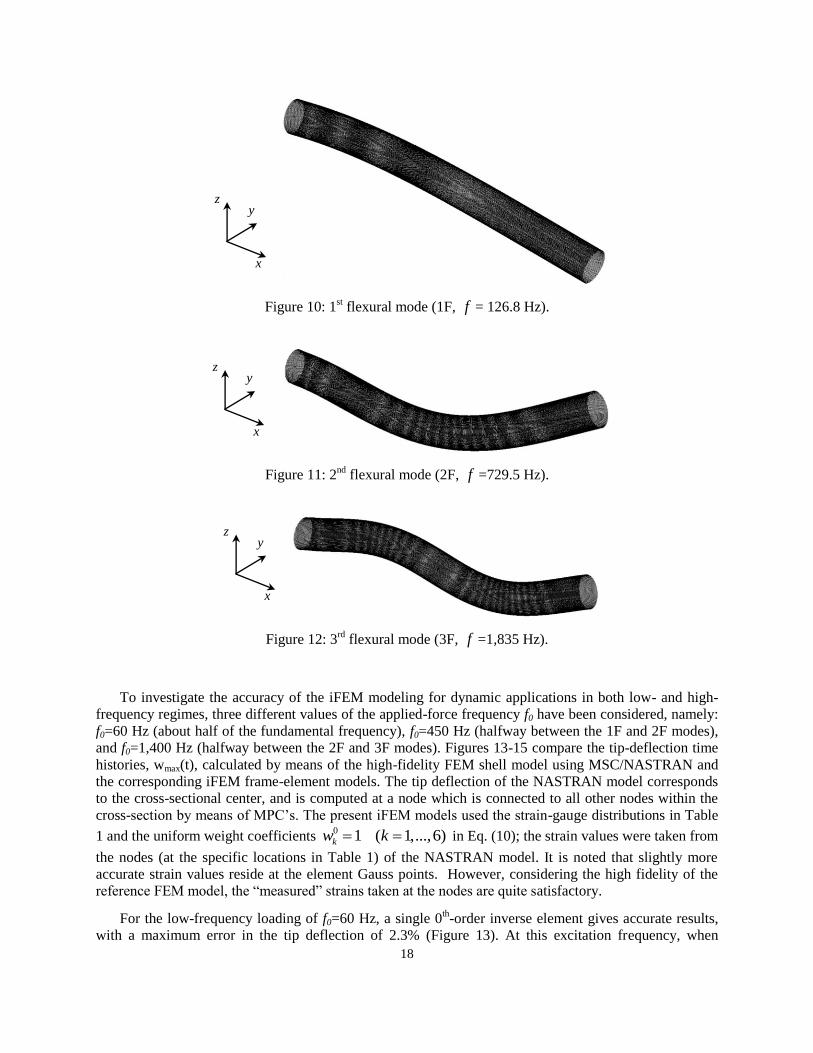
their type, and corresponding frequency value f; the first three flexural mode shapes are shown in Figures
10-12. The other modes in this frequency range are associated with shell modes describing cross-sectional
distortion and are neither shown nor tabulated.
Table 2: Global modes of the cantilevered beam in the frequency range of 0-5,000 Hz. (F-type modes are
flexural; M-type modes are membrane.)
Mode order
1st and 2
nd
modes
3rd
and 4th
modes 12
th mode
13th and
14th modes
30th and
31st modes
40th and
41st modes
Mode type
1F 2F 1M 3F 4F 5F
f frequency
[Hz] 126.8 729.5 1,670 1,835 3,187 4,671
18
Figure 10: 1st flexural mode (1F, f = 126.8 Hz).
Figure 11: 2nd
flexural mode (2F, f =729.5 Hz).
Figure 12: 3rd
flexural mode (3F, f =1,835 Hz).
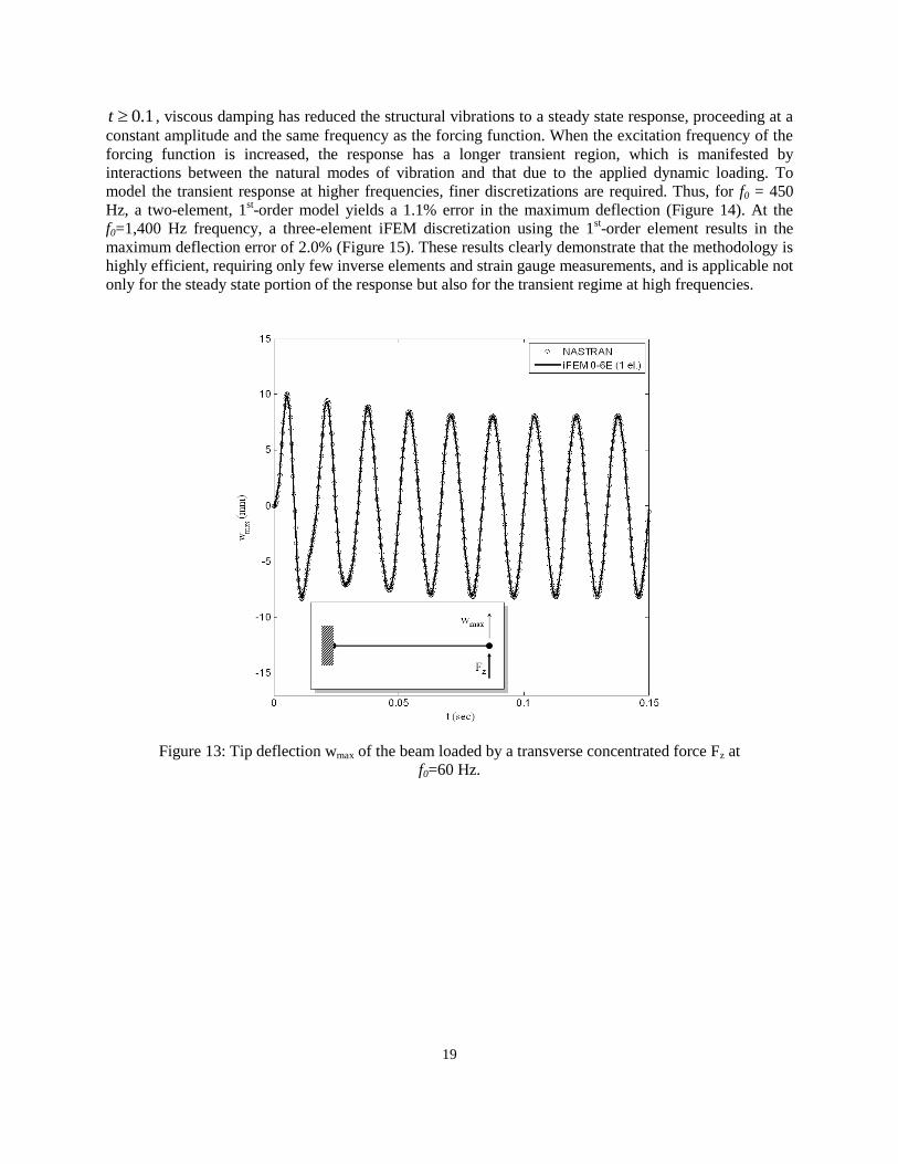
To investigate the accuracy of the iFEM modeling for dynamic applications in both low- and high-
frequency regimes, three different values of the applied-force frequency f0 have been considered, namely:
f0=60 Hz (about half of the fundamental frequency), f0=450 Hz (halfway between the 1F and 2F modes),
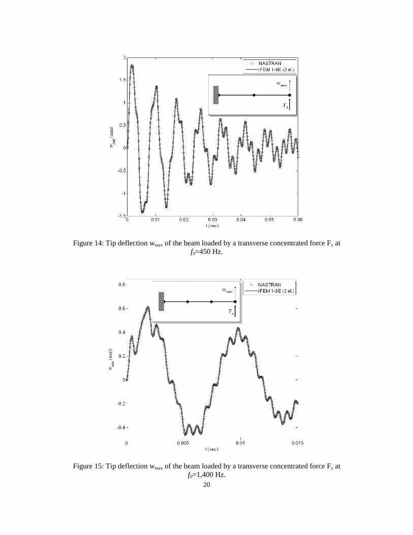
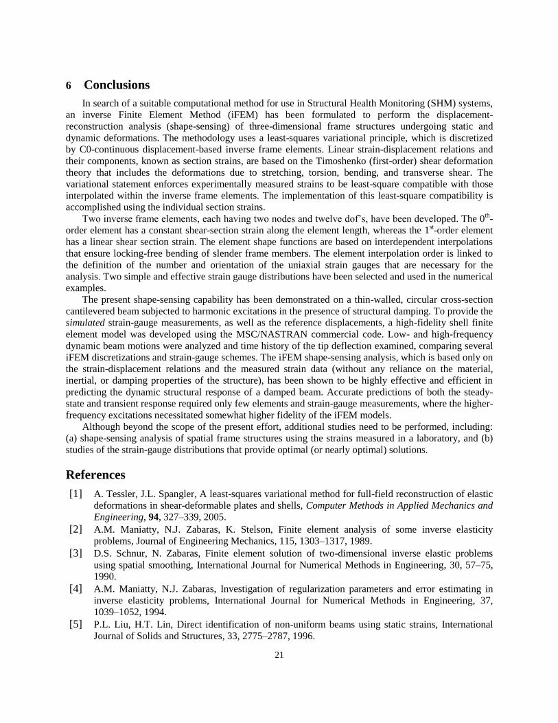
and f0=1,400 Hz (halfway between the 2F and 3F modes). Figures 13-15 compare the tip-deflection time
histories, wmax(t), calculated by means of the high-fidelity FEM shell model using MSC/NASTRAN and
the corresponding iFEM frame-element models. The tip deflection of the NASTRAN model corresponds
to the cross-sectional center, and is computed at a node which is connected to all other nodes within the
cross-section by means of MPC’s. The present iFEM models used the strain-gauge distributions in Table
1 and the uniform weight coefficients 0 1 ( 1,...,6)kw k in Eq. (10); the strain values were taken from
the nodes (at the specific locations in Table 1) of the NASTRAN model. It is noted that slightly more
accurate strain values reside at the element Gauss points. However, considering the high fidelity of the
reference FEM model, the “measured” strains taken at the nodes are quite satisfactory.
For the low-frequency loading of f0=60 Hz, a single 0th-order inverse element gives accurate results,
with a maximum error in the tip deflection of 2.3% (Figure 13). At this excitation frequency, when
z y
x
z y
x
z y
x
19
0.1t , viscous damping has reduced the structural vibrations to a steady state response, proceeding at a
constant amplitude and the same frequency as the forcing function. When the excitation frequency of the
forcing function is increased, the response has a longer transient region, which is manifested by
interactions between the natural modes of vibration and that due to the applied dynamic loading. To
model the transient response at higher frequencies, finer discretizations are required. Thus, for f0 = 450
Hz, a two-element, 1st-order model yields a 1.1% error in the maximum deflection (Figure 14). At the
f0=1,400 Hz frequency, a three-element iFEM discretization using the 1st-order element results in the
maximum deflection error of 2.0% (Figure 15). These results clearly demonstrate that the methodology is
highly efficient, requiring only few inverse elements and strain gauge measurements, and is applicable not
only for the steady state portion of the response but also for the transient regime at high frequencies.
Figure 13: Tip deflection wmax of the beam loaded by a transverse concentrated force Fz at
f0=60 Hz.
20
Figure 14: Tip deflection wmax of the beam loaded by a transverse concentrated force Fz at
f0=450 Hz.
Figure 15: Tip deflection wmax of the beam loaded by a transverse concentrated force Fz at
f0=1,400 Hz.
21
6 Conclusions
In search of a suitable computational method for use in Structural Health Monitoring (SHM) systems,
an inverse Finite Element Method (iFEM) has been formulated to perform the displacement-
reconstruction analysis (shape-sensing) of three-dimensional frame structures undergoing static and
dynamic deformations. The methodology uses a least-squares variational principle, which is discretized
by C0-continuous displacement-based inverse frame elements. Linear strain-displacement relations and
their components, known as section strains, are based on the Timoshenko (first-order) shear deformation
theory that includes the deformations due to stretching, torsion, bending, and transverse shear. The
variational statement enforces experimentally measured strains to be least-square compatible with those
interpolated within the inverse frame elements. The implementation of this least-square compatibility is
accomplished using the individual section strains.
Two inverse frame elements, each having two nodes and twelve dof’s, have been developed. The 0th-
order element has a constant shear-section strain along the element length, whereas the 1st-order element
has a linear shear section strain. The element shape functions are based on interdependent interpolations
that ensure locking-free bending of slender frame members. The element interpolation order is linked to
the definition of the number and orientation of the uniaxial strain gauges that are necessary for the
analysis. Two simple and effective strain gauge distributions have been selected and used in the numerical
examples.
The present shape-sensing capability has been demonstrated on a thin-walled, circular cross-section
cantilevered beam subjected to harmonic excitations in the presence of structural damping. To provide the
simulated strain-gauge measurements, as well as the reference displacements, a high-fidelity shell finite
element model was developed using the MSC/NASTRAN commercial code. Low- and high-frequency
dynamic beam motions were analyzed and time history of the tip deflection examined, comparing several
iFEM discretizations and strain-gauge schemes. The iFEM shape-sensing analysis, which is based only on
the strain-displacement relations and the measured strain data (without any reliance on the material,
inertial, or damping properties of the structure), has been shown to be highly effective and efficient in
predicting the dynamic structural response of a damped beam. Accurate predictions of both the steady-
state and transient response required only few elements and strain-gauge measurements, where the higher-
frequency excitations necessitated somewhat higher fidelity of the iFEM models.
Although beyond the scope of the present effort, additional studies need to be performed, including:
(a) shape-sensing analysis of spatial frame structures using the strains measured in a laboratory, and (b)
studies of the strain-gauge distributions that provide optimal (or nearly optimal) solutions.
References
[1] A. Tessler, J.L. Spangler, A least-squares variational method for full-field reconstruction of elastic
deformations in shear-deformable plates and shells, Computer Methods in Applied Mechanics and
Engineering, 94, 327–339, 2005.
[2] A.M. Maniatty, N.J. Zabaras, K. Stelson, Finite element analysis of some inverse elasticity
problems, Journal of Engineering Mechanics, 115, 1303–1317, 1989.
[3] D.S. Schnur, N. Zabaras, Finite element solution of two-dimensional inverse elastic problems
using spatial smoothing, International Journal for Numerical Methods in Engineering, 30, 57–75,
1990.
[4] A.M. Maniatty, N.J. Zabaras, Investigation of regularization parameters and error estimating in
inverse elasticity problems, International Journal for Numerical Methods in Engineering, 37,
1039–1052, 1994.
[5] P.L. Liu, H.T. Lin, Direct identification of non-uniform beams using static strains, International
Journal of Solids and Structures, 33, 2775–2787, 1996.
22
[6] M.A. Davis, A.D. Kersey, J. Sirkis, E.J. Friebele, Shape and vibration mode sensing using a fiber
optic Bragg grating array, Smart Materials and Structures, 5, 759–765, 1996.
[7] L.H. Kang, D.K. Kim, J.H. Han, Estimation of dynamic structural displacements using fiber Bragg
grating strain sensors, Journal of Sound and Vibration, 305, 534–542, 2007.
[8] N.S. Kim, N.S. Cho, Estimating deflection of a simple beam model using fiber optic Bragg-grating
sensors, Experimental Mechanics, 44, 433–439, 2004.
[9] W.L. Ko, W.L. Richards, V.T. Fleischer, Applications of the Ko displacement theory to the
deformed shape predictions of the doubly-tapered Ikhana wing, NASA/TP-2009-214652, October
2009.
[10] P.B. Bogert, E.D. Haugse, R.E. Gehrki, Structural shape identification from experimental strains
using a modal transformation technique, 44th AIAA/ASME/ASCE/AHS Structures, Structural
Dynamics and Materials Conference, Norfolk, Virginia, 2003.
[11] R.T. Jones, D.G. Bellemore, T.A. Berkoff, J.S. Sirkis, M.A. Davis, M.A. Putnam, E.J. Friebele,
A.D. Kersey, Determination of cantilever plate shapes using wavelength division multiplexed fiber
Bragg grating sensors and a least-squares strain-fitting algorithm, Smart Materials and Structures,
7, 178–188, 1998.
[12] S. Shkarayev, R. Krashantisa, A. Tessler, An inverse interpolation method utilizing in-flight strain
measurements for determining loads and structural response of aerospace vehicles, 3rd
International Workshop on Structural Health Monitoring, Stanford, California, 2001.
[13] S. Shkarayev, A. Raman, A. Tessler, Computational and experimental validation enabling a viable
in-flight structural health monitoring technology, 1st European Workshop on Structural Health
Monitoring, Cachan, Paris, France, 2002.
[14] P. Mainçon, Inverse FEM I: Load and response estimates from measurements, 2nd International
Conference on Structural Engineering, Mechanics and Computation, Cape Town, South Africa,
2004.
[15] P. Mainçon, Inverse FEM II: Dynamic and non-linear problems, 2nd International Conference on
Structural Engineering, Mechanics and Computation, Cape Town, South Africa, 2004.
[16] A.J. Maree, P. Mainçon, Inverse FEM III: Influence of measurement data availability, 2nd
International Conference on Structural Engineering, Mechanics and Computation, Cape Town,
South Africa, 2004.
[17] Barnardo, P. Mainçon, Inverse FEM IV: Influence of modelling error, 2nd International
Conference on Structural Engineering, Mechanics and Computation, Cape Town, South Africa,
2004.
[18] M. Nishio, T. Mizutani, N. Takeda, Structural shape reconstruction with consideration of the
reliability of distributed strain data from a Brillouin-scattering-based optical fiber sensor, Smart
Materials and Structures, 19, 1-14, 2010.
[19] A. Tessler, J.L. Spangler, A variational principal for reconstruction of elastic deformation of shear
deformable plates and shells, NASA TM-2003-212445, August 2003.
[20] A. Tessler, J.L. Spangler, Inverse FEM for full-field reconstruction of elastic deformations in shear
deformable plates and shells, 2nd European Workshop on Structural Health Monitoring, Munich,
Germany, 2004.
[21] S.L. Vazquez, A. Tessler, C.C. Quach, E.G. Cooper, J. Parks, J.L. Spangler, Structural health
monitoring using high-density fiber optic strain sensor and inverse finite element methods, NASA
TM-2005-213761, May 2005.
[22] C.C. Quach, S.L. Vazquez, A. Tessler, J.P. Moore, E.G. Cooper, J.L. Spangler, Structural anomaly
detection using fiber optic sensors and inverse finite element method, AIAA Guidance,
Navigation, and Control Conference and Exhibit, San Francisco, California, 2005.
23
[23] P. Cerracchio, M. Gherlone, M. Mattone, M. Di Sciuva, A. Tessler, Shape sensing of three-
dimensional frame structures using the inverse finite element method, 5th European Workshop on
Structural Health Monitoring, Sorrento, Italy, 2010.
[24] M. Gherlone, P. Cerracchio, M. Mattone, M. Di Sciuva, A. Tessler, Dynamic shape reconstruction
of three-dimensional frame structures using the inverse finite element method, 3rd ECCOMAS
Thematic Conference on Computational Methods in Structural Dynamics and Earthquake
Engineering, Corfù, Greece, 2011.
[25] S.P. Timoshenko, On the correction for shear of differential equations for transverse vibrations of
prismatic bars, Philosophical Magazine, 41, 744–746, 1921.
[26] A. Tessler, S.B. Dong, On a hierarchy of conforming Timoshenko beam elements, Computers &
Structures, 14, 335–344, 1981.
[27] A.I. Lurie, Theory of Elasticity, Springer-Verlag Berlin Heidelberg, New York, 2005.
[28] MSC/MD-NASTRAN, Reference Guide, Version 2006.0, MSC Software Corporation, Santa Ana,
CA.
Appendix A
The 1st, 2
nd, and 4
th-degree Lagrange shape functions are given as
1st degree
(1) (1)
1 2
1, 1 , 1
2L L (A1)
2nd
degree
(2) (2) (2) 2
1 2
1, , 1 ,2 1 , 1
2rL L L
(A2)
4th degree
(4) (4) 2
1 2
(4) (4) (4) 2 2
1, 4 1 1 , 1
6
1, , 1 4 2 1 ,3 1 4 ,4 2 1
3q r s
L L
L L L
(A3)
where 2 / 1 1,1ex L is a non-dimensional axial coordinate; 0, ex L and eL denotes the
element length. The subscripts 1 and 2 represent the end nodes, whereas q, r, and s denote the uniformly
spaced interior nodes.
The 3rd
–degree shape functions, (3)
jN , of the 0th-order element have the form
24
(3) (3) (3) 2
1 2, , 1 2 3 , 4 , 2 324
e
r
LN N N (A4)
whereas the cubic (3)
kN shape functions of the 1st-order element are
(3) (3) (3) (3) (3) 21 2
4, , , , 1 4 3 , 2 8 3 ,24 , 2 8 3 , 4 3
3q r s
eN N N N N
L
(A5)
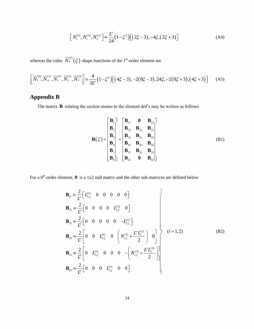
Appendix B
The matrix B relating the section strains to the element dof’s may be written as follows
1 11 12
2 21 2 22
3 31 3 32
4 41 4 42
5 51 5 52
6 61 62
c
c
c
c
B B 0 B
B B B B
B B B BB
B B B B
B B B B
B B 0 B
(B1)
For a 0th-order element, 0 is a 1x2 null matrix and the other sub-matrices are defined below
(1)
1 ,
(2)
2 ,
(2)
3 ,
(2)(1) (3)
4 , ,
(2)(1) (3)
5 , ,
(1)
6 ,
20 0 0 0 0
20 0 0 0 0
20 0 0 0 0
20 0 0 0
2
20 0 0 0
2
20 0 0 0 0
i ie
i ie
i ie
e
ii i ie
e
ii i ie
i ie
LL
LL
LL
L LL N
L
L LL N
L
LL
B
B
B
B
B
B
( 1, 2)i
(B2)
25
(2)
2 ,
(2)
3 ,
(2)(3)
4 ,
(2)(3)
5 ,
20
20
20
2
20
2
c re
c re
e
rc re
e
rc re
LL
LL
L LN
L
L LN
L
B
B
B
B
(B3)
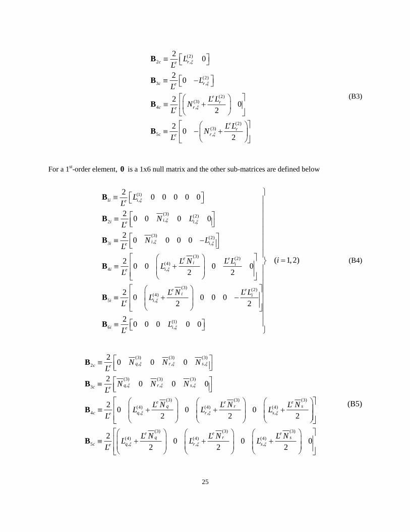
For a 1st-order element, 0 is a 1x6 null matrix and the other sub-matrices are defined below
(1)
1 ,
(3)(2)
,2 ,
(3)(2)
,3 ,
(3) (2)(4)
4 ,
(3) (2)(4)
5 ,
6
20 0 0 0 0
20 0 0 0
20 0 0 0
20 0 0 0
2 2
20 0 0 0
2 2
20 0 0
i ie
ii ie
ii ie
eei i
i ie
eei i
i ie
i e
LL
N LL
N LL
L LL NL
L
L LL NL
L
LL
B
B
B
B
B
B(1)
,
( 1, 2)
0 0i
i
(B4)
(3) (3) (3)
, , ,2
(3) (3) (3)
, , ,3
(3) (3) (3)
(4) (4) (4)
4 , , ,
(3)
(4)
5 , ,
20 0 0
20 0 0
20 0 0
2 2 2
20
2
q r sc e
q r sc e
e e eq r s
c q r se
eq
c q re
N N NL
N N NL
L N L N L NL L L
L
L NL L
L
B
B
B
B
(3) (3)
(4) (4)
,0 02 2
e er s
s
L N L NL
(B5)
REPORT DOCUMENTATION PAGEForm Approved
OMB No. 0704-0188
2. REPORT TYPE
Technical Publication 4. TITLE AND SUBTITLE
Dynamic Shape Reconstruction of Three-Dimensional Frame Structures Using the Inverse Finite Element Method
5a. CONTRACT NUMBER
6. AUTHOR(S)
Gherlone, Marco; Cerrachio, Priscilla; Mattone, Massimiliano; Di Sciuva, Marco; Tessler, Alexander
7. PERFORMING ORGANIZATION NAME(S) AND ADDRESS(ES)
NASA Langley Research CenterHampton, VA 23681-2199
9. SPONSORING/MONITORING AGENCY NAME(S) AND ADDRESS(ES)
National Aeronautics and Space AdministrationWashington, DC 20546-0001
8. PERFORMING ORGANIZATION REPORT NUMBER
L-20096
10. SPONSOR/MONITOR'S ACRONYM(S)
NASA
13. SUPPLEMENTARY NOTES
12. DISTRIBUTION/AVAILABILITY STATEMENTUnclassified UnlimitedSubject Category 39Availability: NASA CASI (443) 757-5802
19a. NAME OF RESPONSIBLE PERSON
STI Help Desk (email: [email protected])
14. ABSTRACT
A robust and efficient computational method for reconstructing the three-dimensional displacement field of truss, beam, and frame structures, using measured surface-strain data, is presented. Known as “shape sensing”, this inverse problem has important implications for real-time actuation and control of smart structures, and for monitoring of structural integrity. The present formulation, based on the inverse Finite Element Method (iFEM), uses a least-squares variational principle involving strain measures of Timoshenko theory for stretching, torsion, bending, and transverse shear. Two inverse-frame finite elements are derived using interdependent interpolations whose interior degrees-of-freedom are condensed out at the element level. In addition, relationships between the order of kinematic-element interpolations and the number of required strain gauges are established. As an example problem, a thin-walled, circular cross-section cantilevered beam subjected to harmonic excitations in the presence of structural damping is modeled using iFEM; where, to simulate strain-gauge values and to provide reference displacements, a high-fidelity MSC/NASTRAN shell finite element model is used. Examples of low and high-frequency dynamic motion are analyzed and the solution accuracy examined with respect to various levels of discretization and the number of strain gauges.
15. SUBJECT TERMS
Frame finite element; Inverse Finite Element Method; Structural Health Monitoring; Timoshenko beam theory; Variational principle
18. NUMBER OF PAGES
30
19b. TELEPHONE NUMBER (Include area code)
(443) 757-5802
a. REPORT
U
c. THIS PAGE
U
b. ABSTRACT
U
17. LIMITATION OF ABSTRACT
UU
Prescribed by ANSI Std. Z39.18Standard Form 298 (Rev. 8-98)
3. DATES COVERED (From - To)
5b. GRANT NUMBER
5c. PROGRAM ELEMENT NUMBER
5d. PROJECT NUMBER
5e. TASK NUMBER
5f. WORK UNIT NUMBER
284848.02.03.07.01
11. SPONSOR/MONITOR'S REPORT NUMBER(S)
NASA/TP-2011-217315
16. SECURITY CLASSIFICATION OF:
The public reporting burden for this collection of information is estimated to average 1 hour per response, including the time for reviewing instructions, searching existing data sources, gathering and maintaining the data needed, and completing and reviewing the collection of information. Send comments regarding this burden estimate or any other aspect of this collection of information, including suggestions for reducing this burden, to Department of Defense, Washington Headquarters Services, Directorate for Information Operations and Reports (0704-0188), 1215 Jefferson Davis Highway, Suite 1204, Arlington, VA 22202-4302. Respondents should be aware that notwithstanding any other provision of law, no person shall be subject to any penalty for failing to comply with a collection of information if it does not display a currently valid OMB control number.PLEASE DO NOT RETURN YOUR FORM TO THE ABOVE ADDRESS.
1. REPORT DATE (DD-MM-YYYY)
12 - 201101-