Dynamic stability evaluation for multimachinesystem: an efficient eigenvalue approach

Z. Elrazaz, B.Sc.(Eng.), B.Sc.(Math.), Ph.D., Mem. I.E.E.E., andProf. N.K. Sinha, B.Sc, Ph.D., C.Eng., P.Eng., F.I.E.R.E., M.C.S.E.E., Sen. Mem. I.E.E.E., M.I.E.E.

Indexing terms: Stability, Power systems and plant

Abstract: A new method is presented for evaluating the dynamic stability of a multimachine power system.The effect of large changes in the system parameters on the eigenpattern is calculated using new formulas forhigher-order eigenvalue sensitivities. The new method requires only a small additional computational effort.

1 Introduction

The evaluation of dynamic stability is necessary for both theplanning and operation of electric power systems. Practicalsystems are large and nonlinear with complex interactions. Toexamine and analyse the dynamic stability of the system, thenonlinear equations describing it are linearised about anoperating point since the dynamic stability is concerned withsmall disturbances in the system. The eigenvalues of thelinearised system matrix are indicative of the system perform-ance [1]. The eigenvalues are related to the different modes ofthe system. Whereas the real part is a measure of the amount ofdamping, the imaginary part is related to the natural frequencyof oscillation of the corresponding mode. System eigenvaluesare, in general, functions of all control and design parameters.The change in any of these parameters affects the systemperformance. Hence, it causes a shift in the whole eigenvaluepattern. The amount of shift depends on the sensitivity of thedifferent eigenvalues to a parameter as well the actual changein the value of that parameter. In order to predict the systemperformance under different parameter settings, the eigen-values should be recomputed for every parameter selection.However, the relatively high order of the system (especially ina multimachine environment) and the multiplicity of par-ameter variation possibilities make it impractical to carry outrepeated eigenvalue computations. Thus a great deal of workhas been done [1—5] in evaluating power system dynamicstability using 1st- and 2nd-order eigenvalue sensitivities withTaylor-series expansion at a nominal parameter's values (basecase). The results presented in References 2—6 demonstratethe advantages of employing eigenvalue sensitivities overrepeated eigenvalues computations. The main advantages arethe reduction in the computation cost and the identificationof different system modes. The inclusion of 2nd-ordersensitivity terms makes it possible to obtain a closer approxi-mation to the changes in the eigenvalues with realistic changesin the parameters. It has been shown [4] that this requiresonly a small additional computational effort. Whereas this isa significant improvement, there exist some cases where sucheigenvalues are related to the system parameters in a nonlinearmanner, and the inclusion of the second order is not sufficientfor adequate approximation [5].

To handle this problem, the authors in Reference 5 pro-posed the use of an inverse iteration method developed byWilkinson [10] and the modification developed by Van Ness[11] for determining accurate eigenvalues with correspondingeigenvectors for different parameter settings. In spite of thedrawbacks of the inverse iteration method, the main questionwhich had not been answered is how one can predict the error

Paper 1583D, first received 9th October 1980 and in revised form 9thJune 1981Dr. Elrazaz is with the Electrical Engineering Department, West VirginiaUniversity, Morgantown, WV 26S06, USA, and Prof. Sinha is with theElectrical and Computer Engineering Department, McMaster University,Hamilton, Ontario, Canada L8S 4L7

in the approximate estimate without calculating the exactvalue. This is necessary in order to decide whether to use theinverse iteration method or not.

It may be pointed out that there is a difference betweenchanging the operating point and changing the design par-ameters. For the former, eigenvalue sensitivity analysis is notvalid, since all steady-state values are correlated. For the latter,however, the application of such analysis is highly useful sincemost of the design parameters are uncorrelated. The ideabehind this paper is to present a comprehensive eigenvalueapproach for evaluating the dynamic stability of a multi-machine system supplying power to both dynamic and staticloads.

2 Formulation of the system matrix and eigenvaluesensitivities

In dynamic stability studies, the set of linearised differentialand algebraic equations describing the system performance aremanipulated in the following form [7]:

0)Pl I = Qx + Ru

where x eRn, y eRp, u e R 9 are the state, the output, andthe input vectors, respectively. Premultiplying eqn. 1 by P " 1 ,one obtains

= Sx + Eu

where

S = Pl Q = E = pl R =

(2)

(3)

By proper partitioning of eqn. 3, the following state equationscan be obtained:

x = Ax + Bu

y = Cx+Du

(4)

(5)

The eigenvalues of the system matrix A are indicative of thedynamic stability. Let a system parameter £ change by A£,which may not be small. A problem of considerable practicalimportance is the determination of the corresponding changeAX,- in a particular eigenvalue Xf. So instead of recomputingthe system eigenvalues, a Taylor-series expansion around anominal value £0 gives

(A?)2

2!

N\(6)

268 0143-7054/81/060268 + 07 $01.50/0 IEEPROC, Vol. 128, Pt. D, No. 6, NOVEMBER 1981

In order to compute AX,-, it is necessary to obtain the differenteigenvalue sensitivities up to the Nth order. Moreover, it isnecessary to obtain the value of N to be used to give anadequate approximation of A\,- for a certain change AS-. Acomplete derivation of all eigenvalue and eigenvectorsensitivities of all orders is given in Reference 6 and the Mh-order eigenvalue sensitivity can be stated as

For this case, one can show that

3"x,-

3S"

i J V - 1

as

yN-2

N(N-\)

• H %

3"~2X,- 32 w,-

N-i

2! y-N-2

iN-i

~N-1

where Xn and

(7)

vv2, . . . , wn are the eigen-values and eigenvectors of AT. It can be seen from eqn. 7 thateach of the eigenvalue sensitivities depends on eigenvalue andeigenvector sensitivities of lower orders. Hence, they can allbe calculated in a sequential manner. Thus it is evident thatthe determination of the higher-order sensitivity terms doesnot involve much additional work. The only other requirementis to obtain partial derivatives of the matrix A with respect tothe parameter %.

3 Computation of successive system matrix derivatives

It is clear from the derivation of the state-space matrices thatthe A matrix is a result of matrix manipulations includinginverse and product of constituent matrices. Therefore thefollowing technique can be used. Differentiating eqn. 3 withrespect to the parameter S, we have

as ~ 3S

Since PP 2 =/(identity matrix),

which gives

(8)

Hence

, dP . 30s+p i

(9)

(10)

Most of the control parameters appear in the Q matrix andseldom in the P matrix. Thus one of the two terms in eqn. 8can be zero. Let 3/*/3£ = 0, so that the TVth derivative of S willbe in the form

Or, in the other case, let

31

" " 1dP<T^_S N(N- 1) b2P3S SS^"1 + JV-22! as2 as

If both the partial derivative terms in eqn. 10 are nonzero, itcan be shown that

as" as asN-l 2!

as" asN (12)

Hence, the derivatives can all be calculated in a sequentialmanner. In evaluating the P'1 matrix, the efficient methodproposed in Reference 8 has been used for the multimachineexample. The matrices P, 3"S/3S" are extremely sparse sothat sparse-matrix techniques [12] can be employed forreducing both the computation and the storage requirements.It should be clear that 3"~jA/d%N~j is an extremely sparsematrix. This drastically reduces the number of multiplicationsneeded to evaluate 3"X/3S" [e.g. the number of multipli-cation to evaluate ( 3 " " M / 3 S""y)( ayw/3 SO will be far belown2N]. It should be clearly understood that this approach is torecompute a subset (10—20%) of the whole eigenpattern andnot the whole set. This subset contains the critical eigenvalueswhich are sensitive to the parameter %. A comparison betweenthis approach and the recomputation of the whole eigenvaluesusing available computer-library eigenvalue routines is given inReference 5.

Returning to eqn. 6, we see that a good approximation tothe actual change AX,- in the eigenvalue X,- will be obtained if asufficiently high value of N is chosen. We shall now considerthe problem of selecting an appropriate value of N consistentwith a specified accuracy. The following eigenvalue trackingprocedure is proposed and will be applied in later Sections.

4 Eigenvalue tracking procedure

To test whether a given value of N will be satisfactory for aspecified accuracy, it is proposed to first calculate the changein the eigenvalues Xl0 and the eigenvectors (direct and trans-posed) for a given variation AS,- in the parameter So • At thenew location of the eigenvalue Xfl just obtained, the TVsensitivities are again calculated. These are then used forcalculating the eigenvalue Xl0 for a backward change AS in theparameter from So + AS to So- The difference between thevalues of X,o and Xl0 is a measure of accuracy of thetruncated Taylor-series approximation. If this error is withinspecified tolerance limits, this may be used for obtaining abetter approximation. On the other hand, if the error is large,the value of N must be increased. Extrapolation is always anill defined and unstable process, and serious problems ariseowing to truncation and round-off errors. Without due careand error analysis, the usefulness of the technique is highlylimited. This is why we believe that an estimate for the error inthe process is essential to decide which value of N to choose. Itshould be emphasised that the nonlinearities with respect tothe parameter S are the main factors in deciding the appro-priate value of N. In power system dynamics, these non-linearities are of linear and inverse natures. The nonlinearitiesin the eigenvalues are implicit functions of the nonlinearities inthe A matrix.

IEEPROC, Vol. 128, Pt. D, No. 6, NOVEMBER 1981 269

Table 1: Eigenvalue tracking for the case when Te = 0.05, and N = 4, \,-0 = — 17.851

ATE

0.010.020.030.04

Percentagechange in TE

20406080

Estimated \ j ,

- 14.39-12 .00- 10.87-11 .97

Estimated \ I 0

-17.853-17 .95- 1 8 . 7-21 .27

Error

0.0020.10.853.42

Exact \ j ,

- 14 .38-11 .85

- 9 . 8 8- 8 . 2 7

The procedure can be summarised in the following steps:(a) formulate the system equations in the state-space form

linearised about an appropriate base operating condition(b) compute the system eigenvalues and the normal and

transposed eigenvectors at the base conditions(c) compute the Mh-order normalised eigenvalue sen-

sitivities with respect to system parameters of interest (startingwith N = 1); if TV is greater than 1, go to step (e)

(d) considering a specific parameter, identify the sensitivesubset of eigenvalues and choose the one(s) to be tracked overdifferent settings of the parameter £

(e) estimate the change in the eigenvalues and the eigen-vectors due to a given (large) change A£ in the parameter %using a Taylor-series expansion and the Mh-order normalisedsensitivities (the sensitivities are normalised in the sense thatthey give directly the shift in the eigenvalue due to a unitchange in the corresponding parameter)

(/) using the updated eigenvalues and eigenvectors at £0 +A£, calculate the Mh-order eigenvalue sensitivities at £0 +A£

(g) take a step A£ in the reverse direction to that in step (e),using a Taylor-series expansion at £0 + A£ to obtain an eigen-value estimate Xfo a t £o + A£ — A£

(h) compare X,o to the exact value Xl0 obtained in step(b). The error obtained is e,o = \o ~ ^io

(/) the best approximate value at £0 + A£ for A,- can betaken as (X,i + e,0/2)

(/) if the error obtained is still larger than the specifiedtolerance, increase the order by one and go to step (c). Itshould be noted that the procedure is recursive in nature, inthe sense that each piece of information obtained at N= J isused for N = J+ 1. In other words, only the Jth term in theTaylor series is required to be computed at TV = J.

synchronousmachine

Applications

5.1 Simplified single-machine infinite busbar withstatic exciter

The proposed procedure is applied to a simple example [6] totrack one of the eigenvalues over a wide range of the excitertime constant. Table 1 shows the results obtained. The errorincluded in such a tracking procedure is also given in the sameTable.

It can be seen from this Table that the error X,o — X,o is agood measure of the error between the actual \ix and itsestimated value.

5.2 Lightly loaded hydraulic generatorThis Section demonstrates the significance of the proposedtechnique in clarifying the interaction between load charac-teristics and the excitation control loop. This is especiallyimportant under light load when a generator with static exciterhas been equipped with a stabiliser designed to improvestability under heavy-load conditions.

Fig. 1 is a single-line diagram of the generator connected toa large interconnected system (represented by an infinitebusbar) through a transmission line. The generator has a staticexciter equipped with a supplementary stabilising signal;governor effects are included. The block diagram of thehydraulic generator is shown in Fig. 2. The terminal busbar

transmissionline

infiniternonlinearlocal load

Fig. 1 Hydrosystem configuration

Machine: 66 MVA, 13.8kV ratingIn p.u. based on machine rating:xad = 0.567, xaQ = 0.33, xKd = 0.087,

xKq — 0 1 4 ' xl= 0.123, xe = 0.4,ra = 0.00279, rf= 0.0035, rKd = 0.02,

rKg = 0.04, H = 4.29 s, PG = 0.2, QG = 0.7,D (damping coefficient) = 0.002Exciter-stabiliser:KE = 200, KQ = 20, TE = 0.002,TQ= 1.4, Tx- 0.33, Tv= 0.033s

Governor:T, = 0.4, T3 = 0.4, Ts = 0.35 s, KG = 0.04

feeds a composite load with its power consumptionrepresented as an exponential function of the busbar voltage.

PL = Kx ifp QL = K2 if«

wherePL = active consumed powerQL = reactive consumed powercp = load active power index (megawatt sensitivity

coefficient)cq = load reactive power index (megavar sensitivity

coefficient)Kx, K2 = constants

The system has 14 states, seven for the synchronous machine,four for the exciter and three for the governor. The set ofequations describing the performance of the system are welldocumented in Reference 10. The generator parameters areshown in Fig. 1.

Before tracking the subset of the eigenvalues which areimportant for this study, it should be noted that the charac-teristics of the local load presented in this system are signifi-cant. If the load approximates constant active powercombined with constant reactance (cp = 0, cq = 2), then thesystem is unstable. The eigenvalue pair corresponding to thesynchronous machine torque angle is 0.204 ± / 8.09. If theload approximates constant impedance (cp = 2, cQ = 2), thenthe system is stable (the eigenvalue pair is — 1.36 ± / 6.54).Thus we know that, for this system, stability is related to thevalue of cp that describes the load characteristics [4].

iwater shaft

'AEr e f

Fig. 2 Block diagram of hydraulic generator

270 IEEPROC, Vol. 128, Pt. D, No. 6, NOVEMBER 1981

1

-

6

132.5 ±j

- 0 . 7 4

702

2

7

-

-70.6

503.0

Table 2: System eigenvalues

3

- 55.45

8

- 30.98

4

-

9

12.06

-1.36

±7

±y

27.14

1.8

5

- 0

10

- 1

.74

.45

0.50r

Base values: PG = 0.2, QQ = 0.7, /»L = 1.25, QL = 1, cp = 2, cQ = 2

-2.500 0.5 1.0 1.5 2.0 2.5megawatt sensitivity coefficient

3.5 4.0 30 35 40

Fig. 3 Re (\lOtU) against cp

Table 2 lists the eigenvalues of the system at specified basevalues. Columns 1-3 are the eigenvalues corresponding to thestator and rotor modes. Zein El-Din and Alden [4] identifiedthe eigenvalue at —0.74 as governor mode; however, ouranalysis shows that as a stabiliser mode. This can be seen bytracking this mode with the stabiliser time constant TQ as willbe shown later.

The eigenvalues corresponding to the AVR (automaticvoltage regulator) are listed in column 4, the exciter incolumns 5—7 and the main torque-angle mode in column 8.The governor modes are listed in columns 9 and 10. Table 3shows the sensitivities of the eigenvalues corresponding to thetorque-angle mode with respect to the active power index ofthe load cp. Fig. 3 illustrates the improved accuracy obtained

0.00

-0.2

5 10 15 20 25stabiliser gain KQ

Fig. 5 Re (\S6) against KQ

by including the 3rd- and the 4th-order sensitivities in trackingthe real part of the torque-angle mode over a wide range ofvalues of cp. Although the normalised 4th-order sensitivity ismuch smaller than the 2nd- and 3rd-order terms, as can beseen from Table 3, for a 100% decrease in cp, we obtain anerror of only 2% when the 4th-order term is retained, whereas,with up to 3rd-order terms, the error is 14%, and retaining upto 2nd-order terms gives an error of 87%. This change in cp

corresponds to changing the load from a constant impedanceto a constant active power combined with a constantreactance.

Figs. 4 and 5 illustrate the movement of the real part of thetorque-angle and the AVR modes, respectively, over a widerange of the stabiliser gain KQ. Using the proposed method for

O.OOr

E-Q50

_ -1.00 \ !

-2J000 5 10 15 20 25

stabiliser gain KQ

Fig. 4 Re (\10> u) against KQ

-1.50

35 400.2 0.6 1.0 14 1.8

stabiliser time constant TQ

Fig. 6 Re f\l0nJ against TQ

2.2 2.6

IEEPROC, Vol. 128, Pt. D, No. 6, NOVEMBER 1981 111

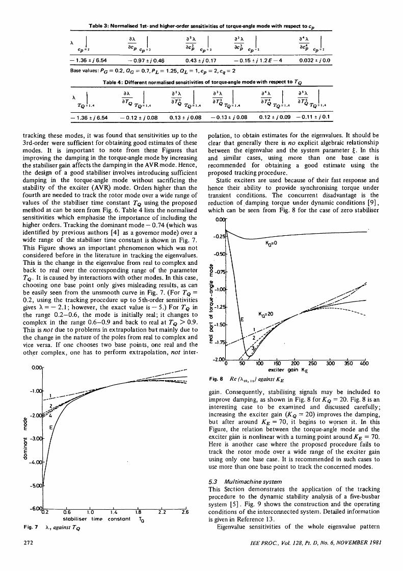
Table 3: Normalised 1st- and higher-order sensitivities of torque-angle mode with respect to cp

dX

— 1.36 + j 6.54 - 0 . 9 7 ±y 0.46 0.43 ±y 0.17 -0.15±y 1.2F-4 0.032 ± j 0.0

Base values: PG = 0.2, QG = 0.7, PL = 1.25, QL= 1,cp = 2 , c q = 2

Table 4 : Different normalised sensitivities of torque-angle mode with respect to

TQ'-I.

3\

3 ^

3 4 \

— 1.36±y'6.54 -0 .12 + /0.08 O.13±yO.O8 -0.13±y'0.08 0.12±y0.09 — 0.11 ±y 0.1

tracking these modes, it was found that sensitivities up to the3rd-order were sufficient for obtaining good estimates of thesemodes. It is important to note from these Figures thatimproving the damping in the torque-angle mode by increasingthe stabiliser gain affects the damping in the AVRmode. Hence,the design of a good stabiliser involves introducing sufficientdamping in the torque-angle mode without sacrificing thestability of the exciter (AVR) mode. Orders higher than thefourth are needed to track the rotor mode over a wide range ofvalues of the stabiliser time constant TQ using the proposedmethod as can be seen from Fig. 6. Table 4 lists the normalisedsensitivities which emphasise the importance of including thehigher orders. Tracking the dominant mode — 0.74 (which wasidentified by previous authors [4] as a governor mode) over awide range of the stabiliser time constant is shown in Fig. 7.This Figure shows an important phenomenon which was notconsidered before in the literature in tracking the eigenvalues.This is the change in the eigenvalue from real to complex andback to real over the corresponding range of the parameterTQ. It is caused by interactions with other modes. In this case,choosing one base point only gives misleading results, as canbe easily seen from the unsmooth curve in Fig. 7. (For TQ =0.2, using the tracking procedure up to 5th-order sensitivitiesgives X = — 2.1; however, the exact value is — 5.) For TQ inthe range 0.2—0.6, the mode is initially real; it changes tocomplex in the range 0.6—0.9 and back to real at TQ > 0.9.This is not due to problems in extrapolation but mainly due tothe change in the nature of the poles from real to complex andvice versa. If one chooses two base points, one real and theother complex, one has to perform extrapolation, not inter-

O.OOr

D.2 0.6 1.0 1.4stabiliser time constant

1.8Tn

2.2 2.6

polation, to obtain estimates for the eigenvalues. It should beclear that generally there is no explicit algebraic relationshipbetween the eigenvalue and the system parameter £. In thisand similar cases, using more than one base case isrecommended for obtaining a good estimate using theproposed tracking procedure.

Static exciters are used because of their fast response andhence their ability to provide synchronising torque undertransient conditions. The concurrent disadvantage is thereduction of damping torque under dynamic conditions [9],which can be seen from Fig. 8 for the case of zero stabiliser

0.00T

-0.25

-2XX)50 100 300 350 400

Fig. 7 \ 7 against TQ

150 200 250exciter gain KE

Fig. 8 Re (Xl0>1J against KE

gain. Consequently, stabilising signals may be included toimprove damping, as shown in Fig. 8 for KQ = 20. Fig. 8 is aninteresting case to be examined and discussed carefully;increasing the exciter gain (KQ = 20) improves the damping,but after around KE = 70, it begins to worsen it. In thisFigure, the relation between the torque-angle mode and theexciter gain is nonlinear with a turning point around KE = 70.Here is another case where the proposed procedure fails totrack the rotor mode over a wide range of the exciter gainusing only one base case. It is recommended in such cases touse more than one base point to track the concerned modes.

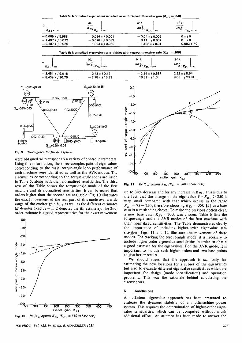
5.3 Multimachine systemThis Section demonstrates the application of the trackingprocedure to the dynamic stability analysis of a five-busbarsystem [5]. Fig. 9 shows the construction and the operatingconditions of the interconnected system. Detailed informationis given in Reference 13.

Eigenvalue sensitivities of the whole eigenvalue pattern

272 IEEPROC, Vol. 128, Pt. D, No. 6, NOVEMBER 1981

X

- 0.66S— 1.407-2 .587

X

- 3.451- 8.439

= 350

> ± 7'±J'±j

2 0 0

±y±7

Table 5: Normalised eigenvalues sensitivities with respect to exciter gain [KEi

ax

KEIKEI- 3 SO

5.988 0.034 ± / 0.0016.072 - 0.076 ± / 0.0899.025 1.003 ± / 0.089

a'x

*K* KE

- 0.04 ±0.11 ±

— 1.198 i

3 50

/ 0.006/ 0.067t 7 0.01

Table 6: Normalised eigenvalues sensitivities with respect to exciter gain (KEl

ax

*KE>KEl = 200

9.018 2.43 ±7 0.1720.75 - 2.78 ± 7 16.29

a'x

""KB*.

- 3 . 5 4 ±16.31 ±

= 200

/ 0.587/1.6

= 350)

= 200)

a'x

2.339.03

= 350

o ± y oo ± y o0.003 ± 7 0

KEl- 2 0 0

± 7 0.94± 7 23.81

%,=O.85*jO.2O %2=0.80*j0.35

Do.6O-jO.O5

^2=0.28^0.08

Fig. 9 Three-generator five-bus system

were obtained with respect to a variety of control parameters.Using this information, the three complex pairs of eigenvaluescorresponding to the main torque-angle loop performance ofeach machine were identified as well as the AVR modes. Theeigenvalues corresponding to the torque-angle loops are listedin Table 5, along with their normalised sensitivities. The thirdrow of the Table shows the torque-angle mode of the firstmachine and its normalised sensitivities. It can be noted thatorders higher than the second are negligible. Fig. 10 illustratesthe exact movement of the real part of this mode over a widerange of the exciter gainA^ as well as the different estimates(E denotes exact, / = 1, 2 denotes the rth estimate). The 2nd-order estimate is a good representative for the exact movement

0.0r

-10.Q200 250

exciter gain450

0.0

-1.0

-2.0

1 -3.0

-5.0

-6.0h

-7.0

2 -8.0I-

-9.0-

-10.0150 200 250 300

exciter gain KE1

"35O~50 100

ig. 11 Re (8 J against KEl (KEl = 200 as base case)

400 450

Fig

Fig. 10 Re (5 J against KEX (KE\ = 350 as base case)

up to 30% decrease and for any increase in KE\ • This is due tothe fact that the change in the eigenvalue for KEi > 250 isvery small compared with that which occurs in the rangeREI = 75 — 250; therefore choosing KEl = 350 [5] as a basecase is a misleading choice. To make the previous notion clear,a new base case, KE1 = 200, was chosen. Table 6 lists thetorque-angle and the AVR modes of the first machine withtheir normalised sensitivities. The Table demonstrates clearlythe importance of including higher-order eigenvalue sen-sitivities. Figs. 11_ and 12 illustrate themovement of thesemodes. For tracking the torque-angle mode, it is necessary toinclude higher-order eigenvalue sensitivities in order to obtaina good estimate for the eigenvalues. For the AVR mode, it isimportant to include such higher orders and two base pointsto give better results.

We should stress that the approach is not only forestimating the new locations for a subset of the eigenvaluesbut also to evaluate different eigenvalue sensitivities which areimportant for design (mode identification) and operationproblems. This was the rationale behind calculating theeigenvectors.

6 Conclusions

An efficient eigenvalue approach has been presented toevaluate the dynamic stability of a multimachine powersystem. This requires the determination of higher-order eigen-value sensitivities, which can be computed without muchadditional effort. An attempt has been made to answer the

IEEPROC, Vol. 128, Pt. D, No. 6, NOVEMBER 1981 273

main question of deciding the maximum order of sensitivitiesto be calculated for a specified accuracy. Three examples ofpower systems with different degrees of complexity have beenconsidered to emphasise the advantages and the limitations ofthe proposed method. The effect of large variations in a par-ameter can be studied with greater confidence withoutrepeating the solution of the eigenvalue problem for the wholesystem. From the examples, it can be seen that a great amountof insight is obtained into the behaviour of the system withlarge parameter variations.

It was observed that sometimes eigenvalues may changefrom real to complex or vice versa with large variations in

' " 50 100 150 200 250 300 350 600 650exciter gain KEJ

F ig. 12 Re (AVRJ against KE,

parameters. The proposed method may give misleading resultsin this case if only one base point is used. In such cases, it issuggested that two base points will give better results. This is

, under further study.

7 References

1 VAN NESS, J.E., BOYLE, J.M., and IMAD, F.P.: 'Sensitivities oflarge mutli-loop control systems', IEEE Trans., 1965, AC-10, pp.308-315

2 NOLAN, P.J., SINHA, N.K., and ALDEN, R.T.H.: 'Eigenvaluesensitivities of power systems including network and shaftdynamics', ibid., 1976, PAS-95, pp. 1318-1324

3 KASTORI, R., and DORARAJU, P.: 'Sensitivity analysis of powersystems', ibid., 1969, PAS-88, pp. 1521-1529

4 ZEIN EL-DIN, H.M., and ALDEN, R.T.H.: 'Second-order eigenvaluesensitivities applied to power system dynamics', ibid., 1977, PAS-96,pp. 1928-1935

5 ZEIN EL-DIN, H.M., and ALDEN, R.T.H.: 'A computer basedeigenvalue approach for power system dynamic stability evaluation'.Proceedings of PICA conference, May 1977, pp. 186-192

6 ELRAZAZ, Z., and SINHA, N.K.: 'Dynamic stability analysis ofpower systems for large parameter variations'. IEEE PES summermeeting, Vancouver, Canada, 15th-20th July 1979

7 ANDERSON, P.M., and FOUAD, A.A.: 'Power system control andstability' (Iowa State University Press, Iowa, 1977)

8 ALDEN, R.T.H., and ZEIN EL-DIN, H.M.: 'Multi-machinedynamic stability calculations', IEEE Trans., 1976, PAS-95, pp.1529-1534

9 DEMELLO, F.P., and CONCORDIA, C: 'Concepts of synchronousmachine stability as affected by excitation control', ibid, 1969,PAS-92, pp. 316-329

10 WILKINSON, J.H.: 'The algebraic eigenvalue problem' (OxfordUniversity Press, 1965), pp. 619-637

11 VAN NESS, J.E.: 'Inverse iteration method for finding eigen-vectors', IEEE Trans., 1969, AC-14, pp. 63-66

12 DUFF, J.S.: 'A survey of sparse matrix research', Proc. IEEE, 1977,65, pp. 500-535

13 ELRAZAZ, Z.: 'Eigenvalue sensitivities applied to power systemdynamics'. Ph.D. dissertation, McMaster University, Hamilton,Ontario, Canada, 1981

274 IEEPROC, Vol. 128, Pt. D, No. 6, NOVEMBER 1981