dynamic structural neutral network - de …chiclana/publications/jifs17-1947.pdf · dynamic...
TRANSCRIPT

1
DYNAMIC STRUCTURAL NEURAL NETWORK
Cu Nguyen Giap1, Le Hoang Son
2,3 *, Francisco Chiclana
4
1Faculty of Management Information System and E-Commerce, ThuongMai University, Hanoi, Viet Nam
2Institute of Research and Development, Duy Tan University, Danang, Viet Nam
3VNU University of Science, Vietnam National University, Viet Nam
4 Centre for Computational Intelligence, School of Computer Science and Informatics, Faculty of
Technology, De Montfort University, Leicester, UK
*: Corresponding author. Tel.: (84) 904.171.284. Address: 334 Nguyen Trai, Thanh Xuan, Hanoi, Vietnam
Abstract: Artificial neural network (ANN) has been well applied in pattern recognition, classification and
machine learning thanks to its high performance. Most ANNs are designed by a static structure whose
weights are trained during a learning process by supervised or unsupervised methods. These training
methods require a set of initial weights values, which are normally randomly generated, with different
initial sets of weight values leading to different convergent ANNs for the same training set. Dealing with
these drawbacks, a trend of dynamic ANN was invoked in the past year. However, they are either too
complex or far from practical applications such as in the pathology predictor in binary multi-input multi-
output (MIMO) problems, when the role of a symptom is considered as an agent, a pathology predictor’s
outcome is formed by action of active agents while other agents’ activities seem to be ignored or have
mirror effects. In this paper, we propose a new dynamic structural ANN for MIMO problems based on the
dependency graph, which gives clear cause and result relationships between inputs and outputs. The new
ANN has the dynamic structure of hidden layer as a directed graph showing the relation between input,
hidden and output nodes. The properties of the new dynamic structural ANN are experienced with a
pathology problem and its learning methods’ performances are compared on a real well known dataset. The
result shows that both approaches for structural learning process improve the quality of ANNs during
learning iteration.
Keywords: Artificial neural network; Binary multi-input multi-output problems; Dynamic structure;
Genetic algorithm; Greedy algorithm; Medical diagnosis.
2
1. INTRODUCTION
Artificial neural network (ANN) has been
applied in numerous areas for a period of time. It
has been widely studied and many ANN models
have been introduced, which are normally
categorized in terms of ANN architectures,
activate functions and learning methods [32].
Most ANNs are designed with a static structure
whose weights are trained during a learning
process by supervised or unsupervised methods
[8]. These training methods require a set of
initial weights values, which are normally
randomly generated, with different initial sets of
weight values leading to different convergence
for the same training set [7]. Even though ANN
is considered a black box that represents a
complex functional relationship between outputs
and inputs, inside information of relation or cross
affection between them is not well
comprehended [33].
Let us consider pathology prediction (aka
medical diagnosis), which is a binary multi-input
multi-output (MIMO) problem, as an example to
illustrate why static structure ANN should be
enhanced. A remarkable area of application of
ANN is pathological expert systems, particularly
in predicting health problems of people from
their precedent symptoms [6]. In this problem,
the appearance or absence of a symptom is
represented by a binary variable and the
prediction result is a binary variable as well. A
feed-forward ANN using back-propagation
learning method is often used therein. Besides,
Deep Neutral Network [6], probability ANN
[27], neuro-fuzzy system [28], etc. have been
utilized alternatively. However, these models
require a large number of iterations in the
training stage and there is no guarantee for its
convergence, especially when using short
training data and a small error is required [4].
Moreover, traditional learning methods treat
each instance of the training dataset the same and
therefore the presence of exceptional inputs
severely influences the ANN error and training
rate [2].
Dealing with these drawbacks, a trend of
dynamic ANN was invoked in the past year.
The term ‘dynamic’ here involves the changes on
the network’s structure or changes on the edges’
weights. Vanini et al. [31] proposed using
dynamic neural networks for fault detection and
isolation in aircraft jet engine. Wu et al. [34]
described a novel method called Deep Dynamic
Neural Networks for multimodal gesture
recognition including a Gaussian-Bernoulli Deep
Belief Network to handle skeletal dynamics, and
3D Convolutional Neural Network to manage
and fuse batches of depth and RGB images. Jin
et al. [14] designed a dynamic neural network for
recurrent calculation of manipulability-maximal
control actions for redundant manipulators under
physical constraints in an inverse-free manner.
Aczon et al. [1] proposed a recurrent neural
network to learn the course of patient encounters.
Amozegar and Khorasani [3] developed an
ensemble of dynamic neural network identifiers
including a dynamic multi-layer perceptron, a
dynamic radial-basis function neural network,
and a dynamic support vector machine.
Gaunt et al. [9] accelerated the Dynamic
Neural Network through Asynchronous Model-
Parallel Training. Mustafa, Allen and Appiah
[18] used Dynamic Multi-Layer Perceptron to
minimize the required computational resource
for an effective mobile-based speech recognition
system. Torabi et al. [29] proposed a dynamic
fuzzy neural network based on sequential fuzzy
clustering for fault diagnosis. It uses Adaptive

3
Neural Fuzzy Inference Systems (ANFIS) to
generate a set of IF-THEN fuzzy rules. After
training, a prune process is applied to eliminate
neurons that are less important or present
redundant fuzzy rules to construct more precise
neural network structure. Online dynamic neutral
networks, on the other way, focus on online
training algorithms.
Pan et al. [22] used both online structure
learning and online parameters learning to form
an efficient online training progress of ANFIS.
They also used an adaptive fuzzy control for
online learning progresses [21, 23]. Pratama et
al. [24-25] proposed condition monitoring
approaches on learning progress, particularly
improving two meta-cognitive what-to-learn and
when-to-learn. They modified the original pClass
by adding a process that initializes new fuzzy
rules from an empty set so that a new model
called pClass+ has the ability to end up with
open and dynamic structure network [26].
Ghiassi et al. [10] proposed a successful
dynamic architecture for Artificial Neural
Networks called DNN2, in which the hidden
layer includes many layers. A layer in the hidden
layer has four nodes fixed but the number of
layers is dynamically determined. This
architecture has been well applied in forecasting
time series events [10] and Pre-Production
Forecasting of Movie Revenues [11]. Inspired by
dynamic structure ANN, Han et al. [12] have
introduced a new dynamic structure neural
network for adaptive dissolved oxygen control
issue. Their approach initializes the hidden layer
with zero or few units and updates the hidden
layer by adding more units during training
process. The other success of using dynamic
structure ANN is presented in [16], where the
authors developed a modification of Weiner-
Type dynamic ANN for Modeling of Nonlinear
Microwave Devices that can be implement in
both software and hardware devices. Other
works regarding the dynamic neural network can
be seen in [17, 19, 20].
Even though there have been recent
advances on the dynamic neural networks, they
are either too complex or far from practical
applications. For example, a pathology predictor
in MIMO problems works like a multi-agent
system in which the combination of each
separate insiders’ activities influences the final
prediction result. In fact, the appearance of a
symptom itself would not be a clear indication
for a specific illness but a set of co-appearance of
symptoms. Moreover, within a set of symptoms
some of them might not strongly belong to a
specific illness; they are just precedents for other
symptoms that directly belong to the true
diagnosed illness. Capturing this aspect, when
the role of a symptom is considered as an agent,
a pathology predictor’s outcome is formed by
action of active agents while other agents’
activities seem to be ignored or have mirror
effects. The current dynamic neural networks are
incapable to model such the cases.
In order to mimic the relationship between
agents in a system, we have to think about a new
dynamic structural ANN model (e.g. for MIMO)
including three layers with the most important
different layer being the hidden layer. The
hidden layer, which is modeled by the
dependency graph, includes the set of nodes
within dynamic adaptive topology. It means that
the structure of the proposed ANN can represent
the relationship between outputs and inputs; and
the structure can be learnt or be updated during
the learning process. By doing so, the dynamic

4
structural ANN is able to handle the variation of
input data as well as the limitations above.
In this paper, we propose a new Dynamic
ANN for binary MIMO problems based on the
dependency graph, which provides clear cause
and result relationships between inputs and
outputs. The dependency graph has been used in
intelligent systems and applications such as
instruction scheduling and job shop scheduling
because it gives a clear relationship between
elements involved in the system [13]. In this
study, the dependency graph is applied in order
to build a dynamic structural ANN that hierarchy
both features of ANN and the dependency graph.
In the new model, the dependency graph is used
as a hidden layer and its topology is trained
during the learning process of ANN.
The rest of paper is organized as follows.
Section 2 describes the proposal dynamic
structural ANN and several proposed learning
methods. Section 3 shows the experimental
results on pathology prediction problem. Finally,
the main results and further works are discussed
in Section 4.
2. DYNAMIC STRUCTURAL ANN
In this section, the new dynamic structural
ANN will be presented and it will be applied to
the pathology prediction problem for illustration
purposes. Specifically, Section 2.1 addresses the
main ideas of the proposed ANN, including its
theoretical validation. Section 2.2 proposes the
design of the new dynamic structural ANN,
while Section 2.3 focuses on two learning
algorithms for the proposed ANN: greedy
algorithm and Genetic Algorithm (GA). Lastly,
Section 2.4 summarizes the advantages of the
proposal against other works.
2.1. Main ideas
Considering pathology prediction as a multi-
agent system, each of its symptoms has a
different impact on a body and their insiders’
activities influence a prediction result. An agent
mimics the action of a symptom or a set of
similar effect symptoms. In fact, the appearance
of a symptom itself might not give an insight
direction for any specific illness because that
symptom may belong to many illnesses. This is
the case with fever, which is a symptom of wide
spread diseases. However, a set of co-appearance
symptoms provides a more confident clue of a
specific illness. Even though the symptoms of an
illness change during the time of such illness, in
its middle stage symptoms are stable. In any
case, within the set of symptoms, some might not
directly belong to an illness; they just are
precedents for other symptoms that directly
belong to a diagnosed illness. This means that
the outcome of pathology prediction is formed
by action of active agents while other agents’
activities seem to be ignored. This relation would
be clearly represented by a dependency graph
[13].
The outcome of a dependency graph is not
evaluated if there is a circular dependency [13].
Indeed, if no specific order is rationally applied
for a circular of dependencies then no object is
calculated first. To overcome this for a
dependency graph, a directed acyclic graph
needs to be formed. Combining features of
dependency graph and properties of a real
pathology diagnosis, a new dynamic structural
ANN is proposed whose structure mimics real
role of symptoms in a disease prediction system.
The proposed new ANN mimics different effects
of an agent to others and different agents’ roles
to the result.

5
In principle, the proposed ANN has three
layers: an input layer, a middle layer, and an
output layer (Fig. 1). Each agent has different
view for input signals and is represented by
different input vectors. The output vector shows
different roles of an agent in a specific economic
factor. The different roles of agents are also
represented by connections between agents.
Therefore, an active agent effect on others can be
represented by high number of nodes
connections, while the output vector can be used
to represent its effect on the output.
Fig. 1. Architecture of static ANN
In the new dynamic structural ANN, the role
of nodes is strongly represented by its topology
of connection rather than connections’ weights.
Therefore, a fixed weight is applied to all edges
to avoid the affection of weight in this type of
ANN. Certainly, it needs to be proved that the
proposed ANN using dynamic topology and a
fixed weight works as the original ANN. Fig. 1
depicts the architecture of a traditional static
ANN.
The existence of an ANN with a single fixed
weight w that works as the above architecture is
proven by replacing a single input iji wx in static
ANN by a sub ANN with single fixed weight w .
As all inputs of a node will be replaced by sub
ANNs that have fixed weight, a static ANN is
transposed into an expected ANN. In this study,
such existence is proved only in case of positive
activation functions. Notice that the most well-
known and applied activation function for ANN
is the sigmoid function, which is a positive
function. Thus, we have the following lemma.
Lemma1. If ANN uses a positive activation
function, a node can be replaced by a sub ANN
having fixed weight.
Proof: Without loss of generality, assume
that input ix has corresponding weight ijw ,
which differs from others. We need to build a
sub ANN having a single weight w for all edges
and prove that there exists a structure of sub
ANN that has single input ix and the ability to
generate same input value iji wx for node j .
Denote by )( wxy i the output of a node
having single input ix and weight w . In the
simplest case, the input iji wx is mimicked by a
sub ANN with ywx iji / nodes as illustrated in
Fig. 2.
Fig. 2. A neuron with fixed weight

6
Node j would be completely replaced by a
sub ANN having fixed weight if all its inputs are
replaced by the same way above. Therefore,
Lemma 1 is proved.
Lemma 2: For each ANN with different
weights, there exists an ANN that has fixed
weight working the same.
Proof: Replacing the nodes in the ANN
with the same structure constructed by Lemma 1
trivially proves this lemma.
However, the question of finding optimal
structure of fixed weighted ANN is still open
herein. Notice that the sigmoid activation
function is both a positive and monotonic
function. The positive monotonic property of
activation functions gives the key point for
searching a suitable topology of dynamic
structural ANN. In the ANN using positive
monotonic activation functions, the relation
between density of structures and output values
is clear since the number of connections does not
decrease. This is summarized in the following
property 1.
Definition 1. Assume two ANNs, A and B,
have the same number of nodes and are
represented by directed graphs without cycle.
Then, B is called a sub ANN of A if all directed
edges in B also appear in A.
Property 1. If an ANN uses a positive
monotonic activation function, its output value is
greater than or equal to those of its sub ANNs.
Proof: We prove that adding an edge to a
given ANN does not decrease the output values.
Given an ANN A that uses a positive monotonic
activation function, without loss of generality,
assume that its node j has a new direct edge
from node i . In this case, the value of jnet is
added, and because the activation function is
positive and monotonic the output of node j
does not decrease. If the output value of node j
is a direct or indirect input of the output node,
the output value of A does not decrease.
Otherwise, node j does not affect the output
node and then the output remains the same.
Remark 1. Property 1 is a consequence of
the following: If B is a sub ANN of A, then A
would be formed by adding one or more edges to
B and therefore the output value of A will be
equal to or greater than that of B. There exists a
limitation of connection between an acyclic
directed graph with a fixed number of nodes.
Therefore, a dynamic structural ANN has a
limited output value.
Definition 2. A network is called a full
connected network if it is represented by a
directed graph that has at least one cycle
providing that any edge is added into this graph.
Remark 2. In an ANN with specific number
of nodes, there is more than one full connected
network. This is because once a full connected
network is obtained by adding edges to the
ANN, the order of adding edges can be changed
to produce a new full connected network. For
example, in a directed graph, if an edge ),( ji is
added, the edge ),( ij cannot be added to avoid
cycle, or in an extension, if two edges ),( ji and
),( kj
are added then edge ),( ik
cannot be
added. Therefore, the order of adding edges leads
to different full connected network.
Property 2. If an ANN has fixed weight and
number of nodes, then output values are upper
bounded.
Proof: Starting from a partial network, i.e. a
not fully connected network, a full connected
network is reached by repeatedly adding an edge

7
into the network. As per Property 1, when an
edge is added, output values do not decrease.
However, with a specific number of nodes, the
number of full connected network is limited.
Therefore, there exits an upper bound for outputs
values and this is generated by the full connected
network having highest output values.
Remark 3. In order to break its upper
bound, a full connected network must increase
the number of nodes. However, in a full
connected network, no more edges can be added.
Therefore, the only way to break through the
upper bound of output values is increasing the
number of node. As soon as new nodes are added
into a dynamic structural ANN, there is a set of
new edges that can be added to increase the
output values.
2.2. Design of the new ANN
From the above idea, we propose a new
ANN that shares several important properties
with the original ANN: the topology of a neuron;
and three layers architecture. However, a
dynamic structural ANN has the following key
differences: every connection between nodes in
the ANN has the same weight; and the hidden
layer is represented by an acyclic directed graph.
Each neuron of a dynamic structural ANN has
multiple inputs, a fixed weight w and one
output with a bias, as depicted in Fig. 3.
Fig. 3. A neuron of dynamic structural ANN
The activation function is sigmoid as
defined below:
(1)
The network architecture has three layers: an
input layer, a hidden layer and an output layer
(Fig. 4):
Input layer: Each input node has
connections to hidden nodes; at least one
connection represented by an input vector iV has
the same weight w .
Dynamic hidden layer:
- One hidden node can connect to any
node in the same layer. The number of
connections of a node shows its effect
on others and, therefore, its indirectly
effect on the output.
- A hidden node having direct connection
to an output j is an active node of j .
A hidden node that does not have direct
connection to an output j is regarded
as a normal/inactive node of j .
- All connections have same weights.
- The hidden layer’s structure shows the
roles of nodes and can be represented
by a directed graph. If a node A has a
directed connection to node B, this
means that output of node A is an input
of node B.
- There is no cycle in a directed graph
that represents the hidden layer.
Output layer:
- The output value depends on the active
hidden nodes’ output.
- An output vector jU represents the
effect of active nodes on the output j ,
and has the same weight.
Output calculation:
- Outputs of NN are calculated through
the activation function and the directed
graph of the hidden layer. As described
b
y

8
in the design, the structure of the hidden
layer aims to avoid any directed cycle
because a cycle will prevent the
calculation process of outputs. In
general, the structure of the hidden layer
must be represented by an acyclic
directed graph.
Fig. 4. Architecture of the proposal ANN
2.3. Learning algorithms
When applying the new dynamic structural
ANN to a real problem, the input and output
layers assign its numbers of nodes according to
the requirement of the problem at hand. The
target of the structural learning process of the
new dynamic structural ANN reduces thus to
learning the structure of the hidden layer. A
directed graph form the structure of all layers
represents the number of nodes and their
connections. Therefore, the leaning algorithm
has to learn a suitable number of nodes and the
topological connections for a training data set.
Learning the structure of ANN is a new learning
process without clear previous instructions [4].
In this section, we propose two approaches
for structural learning. The first one learns
directly by calculating output errors and uses
these errors to update the number of active
hidden nodes based on the Greedy algorithm [5].
Then, back propagation process is applied to
calculate the active hidden nodes, output errors
and update its income connections. This process
repeats until an expected error or maximal
iteration is reached. The second approach uses
Genetic Algorithm (GA) as a key of structural
learning. A set of ANN structures is initialized as
a population, and then using the output errors as
fitness function. The GA will lead to the best
possible structure of the ANN even if it is not a
global optimal structure.
2.3.1. Greedy algorithm
The structure of the hidden layer is learnt
using Property 1 and Property 2: increasing the
number of connections or active nodes in the
hidden layer when using a positive monotonic
activation function leads to increasing the output
values. However, as the network structure forms
a full connection network and a new connection
cannot be added, the only option, according to
Property 2, is to add a new node. The priority
between the two above factors determines the
final resultant structure with high number of
nodes. Therefore, in this section we use the
approach with priority of topological
connections. The designed learning method has
two stages. The first stage initializes the
parameters of the ANN, and the second stage
learns the hidden layer structure by input data
stream.
Stage one
- Randomly initialize a number of hidden
nodes N in the interval [2n- MAX_INT]
where n is the number of inputs,
MAX_INT is the maximum value for a

9
Algorithm 1: Dynamic structure ANN learning
algorithm
Input: a set of training data set 𝑇 = (𝐼, 𝑂), where I is the
set of input instances and O is corresponding output. The
expected error 휀.
Output: a Dynamic structure ANN represented by a
direct graph 𝐺 = {𝑉, 𝐸}{
𝐺 = Init( N, r, w, b)
Do
Foreach 𝑡𝑖 ∈ 𝑇 {
foreach output nodes 𝑗𝑡ℎ {
Calculate the outputs by current structure �̂�𝑗
;
Calculate the outputs error (MMSE): 𝐸𝑗 =
√(�̂�𝑗 − 𝑦𝑗)2;
If (𝐸𝑗 < 휀 ) UpdatingNodeStructure(j,
(�̂�𝑗 − 𝑦𝑗));
Recalculate output error �̂�𝑗;
}
D= TopologicalOdering(hidden layer) ;
Foreach hidden node 𝑖𝑡ℎin reverse order of D
{
𝛿𝑗𝑖 =𝐸𝑗
|𝑁𝑗| ; 𝐸𝑖 = ∑ 𝛿𝑗𝑖
𝑛1
If (Ei > 𝜎)
UpdatingHidenNodeStructure(ith, Ei)
} while (a target error or expected iteration are
reached)
}
Algorithm 2: UpdatingOutputNodeStructure(j,(�̂�𝑗 −𝑦𝑗)) {
If (�̂�𝑗 − 𝑦𝑗)< 0 {
휀𝑚𝑖𝑛 = √(�̂�𝑗 − 𝑦𝑗)2; // min error
a = null; //Hidden node
Foreach ignored node A of 𝑗𝑡ℎ {
If A is active (connects to output node), the
output value changes to 𝑦′̂𝑗 and new error is 𝐸′𝑗 =
√(𝑦′̂𝑗 − 𝑦𝑗)2;
If 휀𝑚𝑖𝑛 > 𝐸′𝑗 then {
휀𝑚𝑖𝑛 = 𝐸′𝑗; a = A; }
}
Ignore node 𝑎 to be active node;
} else {
휀𝑚𝑖𝑛 = √(�̂�𝑗 − 𝑦𝑗)2; // min error
b = null; //Hidden node
Foreach active node B of 𝑗𝑡ℎ {
If turn B into ignored node (not connects to
output node), the output value changes to 𝑦′̂𝑗 and new
error is 𝐸′𝑗 = √(𝑦′̂𝑗 − 𝑦𝑗)2;
If 휀𝑚𝑖𝑛 > 𝐸′𝑗 then {
휀𝑚𝑖𝑛 = 𝐸′𝑗; b = B; }
}
Turn active node 𝑏 into ignored node;
}
}
Algorithm 3 [4]: TopologicalOdering(hidden layer) {
Return a valid topological ordering of the graph
representing the hidden layer using breadth first search
algorithm.
}
Algorithm4: UpdatingHidenNodeStructure(𝑖𝑡ℎ, 𝐸𝑖) {
휀𝑚𝑖𝑛 = 𝐸𝑖; // min error
a = null; //Hidden node
Foreach ignored node A of 𝑖𝑡ℎ {
If A is active (connects to output node), the output value changes to 𝑦′̂𝑖 and new error is 𝐸′𝑗 = √(𝑦′̂𝑖 − 𝑦𝑖)2;
If 휀𝑚𝑖𝑛 > 𝐸′𝑖 then {
휀𝑚𝑖𝑛 = 𝐸′𝑖; a = A; }
}
b = null; //Hidden node
Foreach active node B of 𝑖𝑡ℎ
{
If turn B into ignored node (not connects to output node), the output value changes to 𝑦′̂𝑖 and new error is
𝐸′𝑖 = √(𝑦′̂𝑖 − 𝑦𝑖)2;
If 휀𝑚𝑖𝑛 > 𝐸′𝑖 then { 휀𝑚𝑖𝑛 = 𝐸′𝑖; b = ; }
}
If (b!= null)
Turn active node 𝑏 into ignored node;
Else if (a!= null)
Turn ignored node 𝑎 to be active node;
}

10
32 bit integer and a structure of hidden
layer (with small number of
connections). The number of
connections in the initial structure
should be small in order to capture the
basic information from patterns. A tuple
of bias and weight is also important in
this structural learning, and they are set
by the ANN designer [15]. The bias is
set as high enough, much higher than
the weight, to ensure that the number of
hidden nodes required for a specific
problem is acceptable [15].
Stage two: structural learning process
- In general, minimizing the error of a
trained structural ANN on a specific
training data set is the target of the
structural ANNs’ learning algorithm. In
case of fixed-weight dynamic structural
ANNs, the learning process has to
change the connection between nodes
for better outcome according to
Property 1.
- This stage points out that in an iteration
of learning only active nodes are learnt
directly under the output errors [15].
And then, the active nodes request the
input ones to learn.
Algorithms 1-4 change the connections to
minimize the output errors. The learning
algorithm based on greedy algorithm has rate of
convergence dependent on the characteristic of a
problem. However in one iteration, the learning
algorithm updates all output nodes and continues
the update of relevant active nodes in the hidden
layer. The number of active nodes is Smaller
than or equal to the total number of nodes of the
hidden layer. Updating an active node in worst
case has to update all nodes in the hidden layer.
Update one node is simple task by turning a
selection connection on or off. Therefore, the
complexity of the learning algorithm is
Ο(𝑁, |𝑌|) = (|𝑌| ∙ 𝑁2) where N is the number of
hidden nodes and |𝑌| is the number of output
nodes.
2.3.2 Genetic algorithm
This section uses GA algorithm for learning
the structure of the dynamic structural ANN. In
general, the GA algorithm has four stages. The
first stage initializes a population of problem
solutions. The three remaining stages are
selection, crossover and mutation, which are
repeated until the population converges or a
fixed number of iterations is reached [5]. In order
to use GA algorithm, the first task is to represent
the problem as a chromosome. The structure
indeed includes the number of hidden nodes, the
connections between them and the connections
between hidden nodes and output nodes. Assume
the number of input nodes is 𝑙, the number of
hidden nodes is 𝑛 and the number of output
nodes is 𝑚. The structure of the ANN is
represented by a binary matrix of dimension
(𝑛) ∗ (𝑙 + 𝑛 +𝑚). Each row 𝑖𝑡ℎ of the
matrix represents the out connections of a hidden
node 𝑖𝑡ℎ to other hidden nodes and input, output
nodes. A chromosome to represent the above
structure matrix is a chain with (𝑛) ∗ (𝑙 + 𝑛 +
𝑚) bits [5].
However, this representation of a
chromosome would not guarantee that crossover
generates two new valuable chromosomes for
dynamic structural ANN. The fact is that, a
chromosome must represent an acyclic directed
graph, but the crossover of two chromosomes
would generate new chromosomes that represent

11
a directed graph having cycle. Therefore, a
modification of crossover is introduced here for
dynamic structural ANN. In an acyclic directed
graph, there is an order of nodes and the
connections are fixed from lower rank node to
higher rank node. Therefore, in order to use GA,
all chromosomes have the same order of nodes,
which can be set as {1,2, … , 𝑛} without loss of
generality. New modification of crossover for
dynamic structural ANN has to keep the order of
nodes to guarantee that new chromosomes are
still acyclic directed graph. Subject to this
constraint, the crossover process has to choose
the cut point at the end of the nodes in a
chromosome. In this case, as two chromosomes
exchange their part, the new chromosomes
represent two acyclic directed graphs with the
same order of nodes. The purpose of GA is
finding the network structure that has smallest
error on the training data set. Therefore a fitness
value of a network is estimated by the below
equation (2) where 𝜕𝑗𝑘 is the error of output 𝑗
for an instance of inputs 𝑘. This fitness function
satisfies the requirements of GA: the value of
fitness function is positive and this value
increases when the fitness of solution increases.
𝑓𝑖𝑡𝑛𝑒𝑠𝑠 =1
∑ ∑ 𝜕𝑗𝑘𝑛𝑗=1
𝑚𝑘=1
(2)
Algorithm 5: Genetic Algorithm
Input: a set of training data set 𝑇 = (𝐼, 𝑂), where I is
the set of input instances and O is corresponding
output.
Output: a Dynamic structure ANN represented by a
direct graph 𝐺 = {𝑉, 𝐸} {
Initialization
- Select a number of populations in
initial generation (N, select a fix
number of hidden nodes 𝑛, and
randomly choose an order
𝐷 = {𝑣𝑖} of 𝑛 nodes.
- For each initial structure:
Randomly create a
structure of hidden layer
by randomly choose a
number 𝑧 of connection.
Repeats 𝑧 time: choose
randomly two hidden
nodes 𝐴, 𝐵and create a
connection from 𝐴 to 𝐵,
ensure that A stand
before B in order 𝐷.
While (the error of the best chromosome in current
population larger than target of number of iteration
smaller than expected number)
{
Selection
- Calculate fitness function of all
chromosomes in current
population.
- Using tournament selection
mechanism to select parents set.
Repeats N time the following
progress to choose N parents:
Randomly choose 𝑧
chromosomes form
current population
Select the best
chromosomes to insert
into parents set.
Crossover
- Take randomly two chromosome
from parents set.
- Randomly choose one cut-points.
- Crossover to create two off-
springs.
- Off-springs replace two worst
chromosomes in current
population.
Mutation
- Randomly choose 10%
chromosomes in current
population.
- Randomly switch 10% bits of each
chosen chromosomes.
Choose the best chromosome of the current
population.
}
}

12
There are several remarkable advantages of
the designed GA for NN structure learning
problem. First, the simplicity of chromosome
encryption and the selection, crossover and
mutation mechanisms lead to easy
implementation. Second, the underneath
mathematical process of GAs guarantees to reach
local optimal solution. Third, if an initialized
population of GAs is large enough and diverse,
the final solutions of NN structure will be close
to the global optimum.
However, the most important disadvantage
of GA is computing cost. GA requires
calculating fitness values for all chromosomes of
each generation, and these values are estimated
for all input instances of training set making it
computationally expensive. Reducing the
number of chromosomes or the number of
generations will not solve this issue because they
directly influence to quality of GA. However the
computation time of GA can be reduced by using
Parallel GA [5]. The second disadvantage of GA
is that it works as a “gray-box”, meaning that
although the GA has a clear reaching target, such
as the fitness of a structure for a specific input
set, it does not show the relationship between
fitness convergence and structural change. In
other words, the algorithm does not have a
specific method to change the NN structure
based on target error. The process of GA
algorithm for the dynamic structural ANN is
depicted in Algorithm 5.
In the learning method based on GA, the
rate of convergence is depended on the
characteristics of a problem where it is applied.
However, the complexity of algorithm in one
iteration of GA depends on selection, crossover
and mutation processes.
2.4. Advantages of the proposal
The proposed dynamic structure ANN
differs from other dynamic ANNs mentioned in
the surveyed literature by using a dependency
graph to mapping between multi-inputs and
multi-outputs. In the scope of this paper, we used
fixed weights for any connections between nodes
of the three layers: input layer, hidden layer and
output layer. This approach turns the dynamic
structure into the center of research, where it has
also been proved that a suitable dynamic would
be constructed by a suitable learning process.
Two learning algorithms are used in the new
ANN including the greedy and genetic algorithm
approaches; however in future, new other
efficient learning processes could be
implemented.
The capacity of the proposed dynamic
structure ANN depends on the number of nodes
of the hidden layer that a computing system can
process. Ideally, this number will be extended as
the system need (the number of hidden node will
increase as the size and diversity of data
increase), but in practice, system designers will
have to balance computing time with the number
of hidden units.
3. EVALUATION
This section reports on the experimental
results of the proposed dynamic structural ANN
on training data of heart attack from UCI [30].
The data has 1 output and 22 inputs; the 22
inputs represent the symptoms of patients and
the output is the conclusion about their heart
problem. The training set has 80 instances and
the testing set has 187 instances. In order to
validate the properties of the proposed dynamic
structural ANN, we used the two learning
methods separately and then compare their
accuracy. At first, each learning methods’
performance is tested on the training database to

13
figure out the best parameters, and then, the
results of the two algorithms are compared.
3.1. Greedy algorithm based learning
method
For running the test of greedy algorithm
based learning method, we use different sets of
parameter (N, r, w, b) where N is the number of
hidden node, r is the ratio of initial connections,
w is the weight of connection and b is the bias of
neuron. However, for the purpose of showing the
inside properties of the learning method, we have
run the test with N=100, r=5%, w=0.05, b=0.1.
Each training process runs a maximum of 100
iterations, and the result is estimated by 5 time
testing. The training shows several interesting
results as below.
Instance error during one iteration:
During the iterations of the learning process,
the error of each instance in the training set
varies to balance average errors for all instances.
For example, in the first three iterations, the
errors of training input are shown in Fig.5.
Fig. 5. Learning method performance
Average error vs. number of iteration:
The result shows that the greedy algorithm,
even though designed to improve the quality for
each instance in the training set separately, does
not guarantee convergence to global optimum.
The different instance has affected the ANNs’
structure in deferent ways and a structural
updating improves for one input instance but
reduces results of others (Fig.6).
Fig. 6. Average error during training iteration
3.2. Genetic algorithm based learning
method
We applied GA algorithm with the same
number of hidden node tested by the greedy
algorithm. In general, GA has several important
parameters to test and choose the good
candidate. The number of candidates in
tournament of selection stage is set at 10% of the
population. The rate of mutation is set at 10% of
connection in a chromosome. The performance
of the GA based learning method is shown in
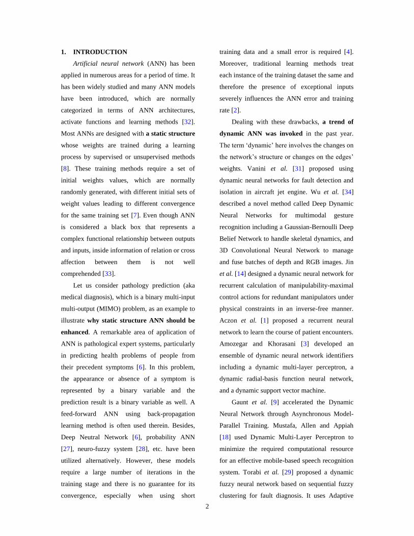
Figs. 7-8. In experience, the algorithm leads to
local convergence after a short number of
iterations. This situation can be improved by
increasing the population size, because a larger
population gives a more diversity generation,
and then the GA will search in larger space, or
increasing the mutation rate [5]. The result
shows the problem of convergence in GA using
tournament selection, with the best chromosome
14
having high possibility to reproduce in next
generation. Besides, we have to limit the number
of cross point selection in the crossover stage;
therefore the searching space is limited. The
consequence is that the GA converges fast to a
local optimum.
Fig. 7. Average testing error vs. number of
population
Fig. 8. Average error in training iteration
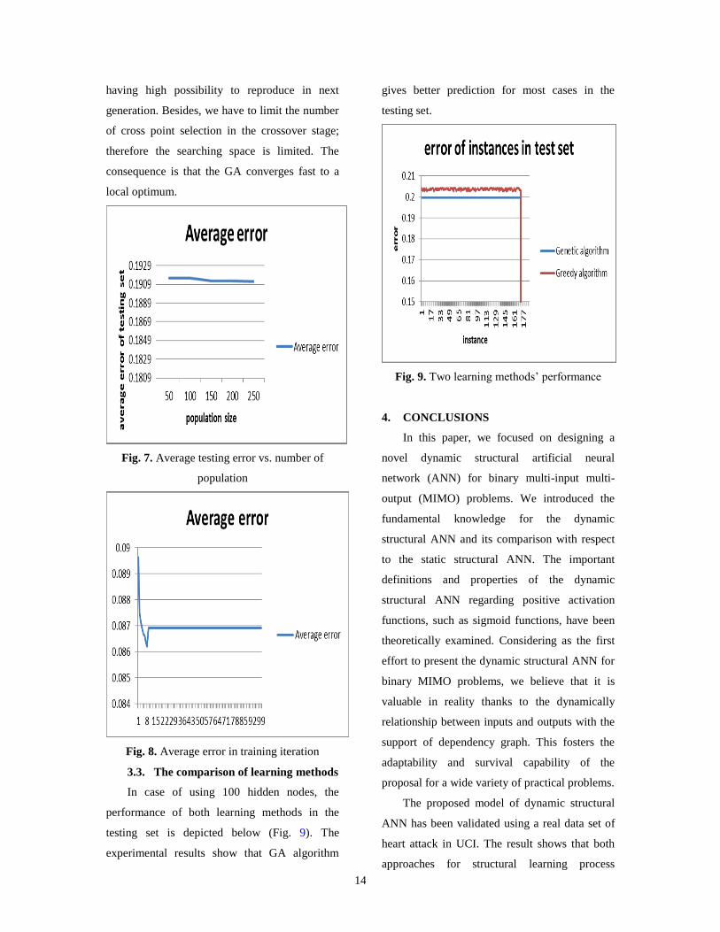
3.3. The comparison of learning methods
In case of using 100 hidden nodes, the
performance of both learning methods in the
testing set is depicted below (Fig. 9). The
experimental results show that GA algorithm
gives better prediction for most cases in the
testing set.
Fig. 9. Two learning methods’ performance
4. CONCLUSIONS
In this paper, we focused on designing a
novel dynamic structural artificial neural
network (ANN) for binary multi-input multi-
output (MIMO) problems. We introduced the
fundamental knowledge for the dynamic
structural ANN and its comparison with respect
to the static structural ANN. The important
definitions and properties of the dynamic
structural ANN regarding positive activation
functions, such as sigmoid functions, have been
theoretically examined. Considering as the first
effort to present the dynamic structural ANN for
binary MIMO problems, we believe that it is
valuable in reality thanks to the dynamically
relationship between inputs and outputs with the
support of dependency graph. This fosters the
adaptability and survival capability of the
proposal for a wide variety of practical problems.
The proposed model of dynamic structural
ANN has been validated using a real data set of
heart attack in UCI. The result shows that both
approaches for structural learning process

15
improve the quality of ANNs during the learning
iteration. In experience, the drawback of both
learning methods is caused by the limitation of
computing power, which curbs for running test
with large number of hidden nodes.
In future, we will expand this research with
other learning methods to construct better results
for the dynamic structural ANN. Large number
of hidden nodes will be tested for better
performance, and suitable areas for applications
of the new dynamic structural ANN to benefit
from the cause and result relationship
represented by the ANN’s structure will be
studied.
ACKNOWLEDGEMENT
This research is funded by Graduate
University of Science and Technology under
grant number GUST.STS.ÐT2017- TT02.
The authors are grateful for the support from
the Institute of Information Technology,
Vietnam Academy of Science and Technology.
We received the necessary devices as experiment
tools to implement proposed method.
REFERENCES
1. Aczon, M., Ledbetter, D., Ho, L., Gunny,
A., Flynn, A., Williams, J., & Wetzel, R.
(2017). Dynamic Mortality Risk Predictions
in Pediatric Critical Care Using Recurrent
Neural Networks. arXiv preprint
arXiv:1701.06675.
2. Amato, F., López, A., Peña-Méndez, E. M.,
Vaňhara, P., Hampl, A., & Havel, J. (2013).
Artificial neural networks in medical
diagnosis. Journal of applied biomedicine,
11(2), pp.47-58.
3. Amozegar, M., & Khorasani, K. (2016). An
ensemble of dynamic neural network
identifiers for fault detection and isolation of
gas turbine engines. Neural Networks, 76,
106-121.
4. Azar, A. T. (2013). Fast neural network
learning algorithms for medical
applications. Neural Computing and
Applications, 23(3-4), 1019-1034.
5. Cantú-Paz, E. (2007). Parameter setting in
parallel genetic algorithms. Parameter
setting in evolutionary algorithms, 259-276.
6. Cireşan, D. C., Giusti, A., Gambardella, L.
M., & Schmidhuber, J. (2013, September).
Mitosis detection in breast cancer histology
images with deep neural networks.
In International Conference on Medical
Image Computing and Computer-assisted
Intervention (pp. 411-418). Springer, Berlin,
Heidelberg.
7. Das, R. (2010). A comparison of multiple
classification methods for diagnosis of
Parkinson disease. Expert Systems with
Applications, 37(2), 1568-1572.
8. Er, M. J., Zhou, M. J. (2008). Automatic
generation of fuzzy inference systems via
unsupervised learning. Neural Networks,
vol. 21, no. 10, pp. 1556-1566.
9. Gaunt, A., Johnson, M., Riechert, M.,
Tarlow, D., Tomioka, R., Vytiniotis, D., &
Webster, S. (2017). AMPNet: Asynchronous
Model-Parallel Training for Dynamic Neural
Networks. arXiv preprint arXiv:1705.09786
10. Ghiassi, M., & Nangoy, S. (2009). A
dynamic artificial neural network model for
forecasting nonlinear processes. Computers
& Industrial Engineering, 57(1), 287-297.
11. Ghiassi, M., Lio, D., & Moon, B. (2015).
Pre-production forecasting of movie
revenues with a dynamic artificial neural
network. Expert Systems with
Applications, 42(6), 3176-3193.

16
12. Han, H. G., & Qiao, J. F. (2011). Adaptive
dissolved oxygen control based on dynamic
structure neural network. Applied Soft
Computing, 11(4), 3812-3820.
13. He, M., & Zhang, J. (2011). A dependency
graph approach for fault detection and
localization towards secure smart grid. IEEE
Transactions on Smart Grid, 2(2), 342-351.
14. Jin, L., Li, S., La, H. M., & Luo, X. (2017).
Manipulability optimization of redundant
manipulators using dynamic neural
networks. IEEE Transactions on Industrial
Electronics, 64(6), 4710 – 4720.
15. Keysers, C., & Gazzola, V. (2014). Hebbian
learning and predictive mirror neurons for
actions, sensations and emotions. Phil.
Trans. R. Soc. B, 369(1644), 20130175.
16. Liu, W., Na, W., Zhu, L., Ma, J., & Zhang,
Q. J. (2017). A Wiener-Type Dynamic
Neural Network Approach to the Modeling
of Nonlinear Microwave Devices. IEEE
Transactions on Microwave Theory and
Techniques.
17. Mohammed, A. M., & Li, S. (2016).
Dynamic neural networks for kinematic
redundancy resolution of parallel Stewart
platforms. IEEE transactions on
cybernetics, 46(7), 1538-1550.
18. Mustafa, M. K., Allen, T., & Appiah, K.
(2017). A comparative review of dynamic
neural networks and hidden Markov model
methods for mobile on-device speech
recognition. Neural Computing and
Applications, 1-9.
19. Nanda, T., Sahoo, B., Beria, H., &
Chatterjee, C. (2016). A wavelet-based non-
linear autoregressive with exogenous inputs
(WNARX) dynamic neural network model
for real-time flood forecasting using
satellite-based rainfall products. Journal of
Hydrology, 539, 57-73.
20. Neubig, G., Dyer, C., Goldberg, Y.,
Matthews, A., Ammar, W., Anastasopoulos,
A., ... & Duh, K. (2017). DyNet: The
Dynamic Neural Network Toolkit. arXiv
preprint arXiv:1701.03980.
21. Pan , Y., Er, M. J., Huang, D., Wang, Q.
(2011). Adaptive fuzzy control with
guaranteed convergence of optimal
approximation error.IEEE Transactions on
Fuzzy Systems, 19 (5), 807-818.
22. Pan , Y., Er, M. J., Li, X., Yu, H., Rafael, G.
(2014). Machine health condition prediction
via online dynamic fuzzy neural networks.
Engineering Applications of Artificial
Intelligence,35, 105-113.
23. Pan, Y., Yu, H. (2016). Biomimetic hybrid
feedback feedforward neural-network
learning control. IEEE Transactions on
Neural Networks and Learning Systems, 28
(6), 1481-1487.
24. Pratama, M., Dimla, E., Lughofer, E.
(2017). Metacognitive Learning Approach
for Online Tool Condition Monitoring.
Journal of Intelligent Manufacturing, 2017.
25. Pratama, M., Lughofer, E., Anavatti, S.,
Lim, C. P. (2017). Data driven modelling
based on recurrent interval-valued
metacognitive scaffolding fuzzy neural
network. Neurocomputing, 2017.
26. Pratama, M., Lughofer, E., Lim, C. P.,
Rahayu, W., Dillon, T., Budiyono, A.
(2017). pClass+: A novel evolving semi-
supervised classifier. International Journal
of Fuzzy Systems, DOI: 10.1007/s40815-
016-0236-3.
27. Shanbhag, S. S., Udupi, G. R., Patil, K. M.,
& Ranganath, K. (2014). Quantitative

17
analysis of diffusion weighted MR images
of brain tumor using signal intensity
gradient technique. Journal of medical
engineering, 2014.
28. Son, L.H., Linh, N. D., & Long, H. V.
(2014). A lossless DEM compression for
fast retrieval method using fuzzy clustering
and MANFIS neural network. Engineering
Applications of Artificial Intelligence, 29,
33-42.
29. Torabi, A. J., Er, M. J., Li, X., Lim, B. S.
(2016). Sequential fuzzy clustering based
dynamic fuzzy neural network for fault
diagnosis and prognosis.
Neurocomputing,vol. 196, pp. 31-41.
30. UCI 2015“Heart Attack dataset,” Available
at:
https://archive.ics.uci.edu/ml/datasets/Heart
+Disease(Accessed on: September 15,
2015).
31. Vanini, Z. S., Khorasani, K., & Meskin, N.
(2014). Fault detection and isolation of a
dual spool gas turbine engine using dynamic
neural networks and multiple model
approach. Information Sciences, 259, 234-
251.
32. Walczak, S. (2018). Artificial neural
networks. In Encyclopedia of Information
Science and Technology, Fourth
Edition (pp. 120-131). IGI Global.
33. Witten, I. H., Frank, E., Hall, M. A., & Pal,
C. J. (2016). Data Mining: Practical
machine learning tools and techniques.
Morgan Kaufmann.
34. Wu, D., Pigou, L., Kindermans, P. J., Le, N.
D. H., Shao, L., Dambre, J., & Odobez, J.
M. (2016). Deep dynamic neural networks
for multimodal gesture segmentation and
recognition. IEEE transactions on pattern
analysis and machine intelligence, 38(8),
1583-1597.