dynamic trading: price inertia and front-runningskrz/dynamic_trading.pdf · dynamic trading: price...
TRANSCRIPT

Dynamic Trading: Price Inertia and Front-Running∗
Yuliy SannikovGraduate School of Business
Stanford University
Andrzej SkrzypaczGraduate School of Business
Stanford University
December 7, 2016
Abstract
We build a linear-quadratic model to analyze trading in a market with pri-vate information and heterogeneous agents. Agents receive private taste/inventoryshocks and trade continuously. Agents differ in their need for trade as well asthe cost to hold excessive inventory. In equilibrium, trade is gradual. Tradingspeed depends on the number and market power of participants, and tradeamong large market participants is slower than that among small ones. Pricehas momentum due to the actions of large traders: it drifts down if the sell-ers have greater market power than buyers, and vice versa. The model canalso answer welfare questions, for example about the social costs and benefitsof market consolidation. It can also be extended to allow private informationabout common value.
1 Introduction.
A market with heterogeneous investors – large institutions, small retail investors,liquidity providers and high-frequency traders – presents many puzzles. What de-termines the speed of trading? What is the link between microstructure and timeseries properties of prices, such as momentum and excess volatility? What is theprice impact of large trades, and how much does it matter for optimal execution oftransactions? What about phenomena such as front-running – are they detrimental
∗We are grateful to seminar participants at Yale, the New York Fed, Cambridge, Stanford,Latin American Econometric Society Meetings, LBS, Harvard, MIT, Northwestern, Chicago, NYU,Georgetown, Duke, the University of Helsinki, the University of Lausanne, Caltech, Collegio CarloAlberto and Universidad de Chile for helpful comments. We are also grateful for research assistanceof Erik Madsen, Giorgio Martini, and Sergey Vorontsov
1

to welfare? What about high frequency trading? Is it justified that in practice, cer-tain market-makers are willing to pay to distinguish institutional trading flow fromthat of retail investors?
We attempt to build a game theoretical framework to analyze these phenomena.Specifically, we model a market in which the price of a risky asset follows a Brownianpath as a result of trades of individual market participants. Trade can be motivated byvarious reasons, such as risk sharing in Vayanos (1999) or because of heterogeneousbeliefs as in Kyle, Obizhaeva and Wang (2014). Players have private informationabout their personal desire to buy or sell at any price, and they trade, optimizingbetween the price at which they trade and the costs of delayed execution. Thus,from the perspective of an individual, our decision makers are similar to a traderin Almgren and Chriss (2001). This classic financial mathematics paper solves theproblem of a trader who decides how quickly it wants to sell a desired quantity, facingthe trade-off between price impact and uncertainty in the execution price. Fast saleslead to a low execution price, but waiting exposes the player to price risk that theplayer is trying to offload. This problem is motivated by basic empirical observationsabout the price impact of trade.
While individual players in our model face a problem similar to that of Almgrenand Chriss (2001), we aim to derive the properties of the market that individualsface from the interaction of individual behaviors. That is, we show that these marketproperties can be derived in a game theoretic framework and we link the price impactof trades as well as time series properties of prices to the composition of the market.
The price properties we derive can be broadly classified as “on-equilibrium” and“off-equilibrium” (path). On equilibrium, we would like to know how prices behavewhen everybody follows their optimal strategies. One important on-equilibrium prop-erty we derive is momentum, which depends on the relative competitiveness/marketpower of current buyers and sellers. Off equilibrium, putting ourselves in the shoesof an individual player, we would like to know how prices would respond if the playertraded differently, not according to the optimal strategy. Of course, the optimalstrategy depends on the off-equilibrium properties of prices, i.e. the price impact thatvarious trades would have. That is, equilibrium strategies have to be optimal giventhe properties of prices off equilibrium. Off equilibrium, we show that as (assumed)in Almgren and Chriss (2001), trades have “instantaneous” and “permanent” priceimpacts, i.e. price depends on the trading rate as well as the total amount bought orsold. In addition, depending on market composition, there may also be “transient”price impact, i.e. the temporary impact on the price of the total amount sold. Tran-sient impact exists empirically, and in our model it arises because transactions by anindividual player trigger trade among other players.1
The dichotomy between on and off-equilibrium phenomena translates to the typesof data that one needs to test various hypothesis empirically. On equilibrium, one
1For empirical research on price impact in equity markets see for example Almgren et al (2005),Moro et al (2009) and a summary in Bouchaud (2010).
2

simply needs the time series data of actual market transactions. The data for off-equilibrium phenomena is much less readily available, and ideally would involve ex-periments by banks that record how prices react depending on the rates of trade.
Game-theoretic justifications of price impact go back to the classic paper of Kyle(1985), where the market maker tries to filter out private information from the com-bined trades of noise traders and an informed trader. Kyle’s “lambda” capturesthe permanent price impact of trades based on the private information that theycarry. A large literature that uses noise traders includes Kyle (1989), Back (1992)and Caldentey and Stacchetti (2010).
Our model builds upon the seminal paper of Vayanos (1999), which models asymmetric market of fully rational traders who have private information about theirdesire to buy or sell. It is a finite market in which trade takes time, as players signaltheir supply or demand by the rate of trading.2 Slow trade leads to inefficiency, astransactions have both instantaneous and permanent price impacts. On equilibriumprices have no momentum when there is symmetry among players. A number ofrecent papers work within such a symmetric framework. Du and Zhu (2013) studythe impact of the frequency of trade on efficiency, and explore how the speed of tradedepends on the amount of private information in the market. Kyle, Obizhaeva andWang (2014) introduce belief heterogeneity, study the speed of trade and observephenomena related to “flash crashes.”3
We introduce asymmetry among players into this class of models. Players dif-fer in their risk capacity parameter that determines their impatience to trade. Werefer to traders who prefer to trade quickly due to a high holding cost as “small”and players who are willing to wait and tolerate execution risk as “large.” As weshow, heterogeneity of traders brings many important issues to the table, but alsosignificantly complicates the modeling task. Unlike in symmetric models, price is nolonger a sufficient statistic about the private information of others; to optimize, eachplayer wants to know the distribution of trades across large and small players. Whenthis information is unavailable, optimization of individual players involves a filteringproblem to infer the distribution of supply and demand from price behavior, and toforecast future price momentum from that distribution. With awareness that sucha framework leads to a host of new phenomena that may be difficult to disentangle,we design a trading mechanism based on the assumption that players know and cancondition on the trades of all other participants.
Our model of trade for asymmetric environments coincides with that of Vayanos(1999) in symmetric case, but otherwise corresponds to the assumption that tradingflow is not anonymous. Our model of trade presents a simple analytical framework- we derive a fully separating equilibrium in which players signal their private in-
2That traders signal by choosing how much to trade is familiar from the static models like Lelandand Pyle (1977) or Myers and Majluf (1984).
3A few papers also study static trading with heterogeneous strategic traders; see for exampleLambert, Ostrovsky and Panov (2016) and Malamud and Rostek (2014).
3

formation about their desire to trade through individual trading flows. We think ofour model as an important benchmark - through which we can identify a host ofphenomena without the complications of belief formation. Also, as in any separat-ing equilibrium, our characterization is invariant to the distribution of shocks to theplayers’ trading needs, and it is even invariant to the correlation among the shocks.A tractable framework for the analysis of markets with heterogeneous participants isa methodological contribution of this paper.
An important implication of heterogeneity is that, when trading is not anonymous,not only trading speed but also price impact depend on player size. Patient/largeplayers are willing to trade slowly, as for any quantity they want to sell they have lowerholding costs than small players. Hence, trades of large players are more “toxic:” theygenerate price momentum that is detrimental to anyone on the other side of the trades.While these observations hold regardless of whether the source of trades is observable,observability implies that the trades of large players have larger instantaneous priceimpact, i.e. the same quantity generates a bigger change in price. In practice thisleads to a variety of behaviors, as players try to obtain information about the sourceof trade. In the popular press, Patterson (2012) and Lewis (2014) document howhigh-frequency traders use “latency tables” and “router signatures” to identify thesource of flow. Certain market makers, such as Citadel, pay retail brokerages forflow from their investors - the knowledge about the source of the flow seems hugelyvaluable. Phenomena such as technical front-running are related to identifying largetraders.
We show that when the source of trades is observable, instantaneous price impacthas a large sensitivity to player size. A trader who is 10 times as large as anothertrader can have instantaneous price impact that is 3 times as large. Of course, inpractice techniques such as splitting of orders allow large traders to hide flow behindthat of small traders at least temporarily. However, recent developments in highfrequency trading and the general push for transparency in markets move realitycloser to our model.4 The question about the role of transparency is important, butit would be a subject of a separate paper.
Since we explicitly model preferences of all market participants, our model can bea laboratory for studying welfare. Here we find several surprising results. First, withtransparency, market power is bad for individual welfare. Market power refers to theability of a large institution to coordinate its trades, avoiding the competition thatwould occur if correlated trades were initiated by many dispersed traders. Marketpower implies slower trades, but it also leads to higher price impact in a transparentmarket of rational traders who can identify a “whale in the ocean.” We present aset of results, demonstrating that large players may prefer to commit to faster trade,and would benefit from being split into smaller traders. These results potentially
4For example, NYSE has a set of liquidity programs that allows retail orders to beidentified as such, in order to generate greater transparency and price improvement - seewww.nyse.com/markets/liquidity-programs.
4

explain the frustration of large institutions with high frequency traders who try tobenefit from identifying large traders, described in Lewis (2014).5 They suggest thattransparent markets may skew the field in favor of small traders, whereas in opaquemarkets large players are able to hide trades behind those of small traders successfully,and benefit from market power.6
This paper is organized as follows. Section 2 presents the linear-quadratic model oftraders’ preferences, a conditional double auction, and equivalence results for differentrepresentations of trading rules. Section 3 describes equilibrium conditions and intro-duces a model of a competitive fringe. Section 4 provides closed-form characterizationof equilibrium in the case of a single large trader and a competitive fringe, discussingon and off path dynamics, as well as welfare properties of the market. Section 5discusses the general case of N asymmetric traders and includes approximations toequilibrium strategies. It also expands discussion of technical front-running. Section6 briefly illustrates how the analysis could be extended to common values. Section 7discusses our findings and Section 8 concludes. Some of the proofs are in the maintext of the paper and some of them are relegated to the appendix. The appendixalso contains a microfoundation of linear-quadratic preferences with a CARA-utilitymaximizing traders.
2 The Model.
Consider a market for a single divisible asset. There are either N large traders, orN − 1 large traders and a “competitive fringe” of infinitely many small players. Wemodel the players’ incentives to trade by following financial mathematics literature.While that literature takes the price impact as given, in our model the equilibriumendogenously determines the magnitude and form of the price impact. We startwith a brief review of a classic paper from this literature, in order to facilitate theinterpretations of the stylized features of the linear-quadratic model that we buildlater.
Background: Price Impact and Optimal Execution. Almgren and Chriss(2001) build an elegant model of optimal execution of transactions, which takes intoaccount the trade-off between average price and execution risk. The trader would liketo liquidate X0 shares and the execution price is modeled as
pt = p0 + σ zt − I qt − Λ
∫ t
0
qs ds, (1)
5Budish, Cramton and Shim (2015) analyze the race for speed in financial markets. Their insightsabout the effects of high frequency trading are unrelated to ours since the two models feature verydifferent trading frictions (speed vs. private information).
6While the impact of transparency on the welfare of large traders relative to small traders seemsclear, the overall impact may be ambiguous. Certainly, identification of large traders that forcesthem to trade slower may reduce market liquidity overall.
5

where p0 is the price at time 0 and zt is a Brownian motion (so σ is the volatility of theprice). The selling rate qt has an instantaneous price impact of I and the permanent
price impact of Λ.7 Once the transaction is completed, i.e. X0 =∫ T
0qt dt, the revenue
equals y =∫ T
0ptqt dt. The objective is to maximize E[y] − γ Var[y]. This objective
function can be justified as a quadratic approximation of a concave utility function:if the trader consumes his wealth w plus y at time T, receiving utility u(w+ y), then
E[u(w + y)] = u(w) + u′(w)E[y] +u′′(w)
2Var[y] + o(y2).
An equivalent way to write the objective function is in terms of quadratic holdingcosts, as shown by the following lemma.
Lemma 1 For deterministic strategies qs, s ∈ [0, T ] that liquidate the amount
X0 =∫ T
0qs ds,
E[y]− γ Var[y] = E[y]− γσ2E
[∫ T
0
X2t dt
], where y =
∫ T
0
ptqt dt (2)
is the seller’s revenue.
Proof. Total revenue equals
y = E[y] +
∫ T
0
Xt σdzt,
where the integral measures the unexpected capital gains and losses on the remainingholdings (notice that if we had σ = 0, then the path of prices would be deterministicfor any deterministic strategy, so y = E[y]). Hence,
Var[y] = σ2 Var
[∫ T
0
Xt dzt
]= σ2 E
[∫ T
0
X2t dt
],
where the last step is just the classic Ito isometry. This implies (2).
In our model below, we model the player’s preferences via quadratic holding costs.Thus, preferences in our model are similar to those of Almgren and Chriss (2001),and they approximate risk-averse utility. We microfound quadratic costs further inAppendix A.8
7Parameter Λ is analogous to Kyle (1985)’s lambda, as it measures the sensitivity of price to thetotal quantity sold.
8We should also note that the characterization of optimal trading in Almgren and Chriss (2001)holds in the class of deterministic strategies, but not in the class of stochastic strategies (whichallow the traders to improve upon the objective E[y]− γVar[y] by “burning money”). However, forpreferences expressed in terms of quadratic holding costs, the deterministic strategy is optimal evenwhen stochastic strategies are allowed.
6

Our Model: Preferences and Shocks. Our model is consistent with thisframework - each of our N players has private information about their desire to buy orsell and chooses how to execute its trade.9 Players have quasilinear utilities in moneyand quadratic holding costs, as in (2). Player i’s desire to buy or sell is captured bya private taste shock ξit ∈ R - the holding cost is quadratic in the difference betweenplayer i’s position xit and the “bliss point” ξit ∈ R – i.e. the holding cost is
− bi2
(xit − ξit
)2. (3)
This formulation is the same as in Bank, Soner and Voß (2016) and Almgren andLi (2016), who capture the costs of an imperfect hedge, except that we also assumethat players discount payoffs (3) at rate r > 0. There are many interpretations.The trader may be a hedge fund manager whose overall risk exposure can affect theoptimal holdings of the asset being traded. Likewise, firms can trade to hedge theircommodity price or currency risk exposure. Alternatively, as in Kyle, Obizhaeva andWang (2014), shocks to ξit could be belief shocks: the trader’s beliefs about the asset’s“alpha” may change and that would affect his optimal holding of the asset. Finally, iftraders are brokers executing trades on the behalf of their clients, then ξit can reflectthe inventory held by the broker.
Parameter bi reflects the holding cost of player i. We interpret 1/bi as the “riskcapacity” of trader i. Players with a lower coefficient bi are “larger”: they can holdlarger positions away from their optimal point ξit at a lower cost. Conversely, playerswith a higher coefficient bi are “smaller”, and therefore more impatient to tradetowards their optimal points.10
We call X it ≡ xit−ξit ∈ R the inventory or allocation of player i. Inventories change
due to taste shocks and trades. Taste shocks have mean 0. For concreteness we takethe taste shocks to be Brownian, so that the vector of taste shocks follows
dξt = −Σ dZt, (4)
where Σ is an N × N matrix with full rank and Z is a vector of N independentBrownian motions. Denote the selling rate of player i by−dxit/dt = qit ∈ R. The vectorof selling flows qt = [q1
t , q2t , . . . , q
Nt ]T must satisfy market clearing, i.e. its coefficients
have to add up to 0. Due to taste shocks and trades, the vector of inventoriesXt = [X1
t , X2t , . . . , X
Nt ]T follows
dXt = Σ dZt − qt dt. (5)
9There is a single asset, but our model can be extended to multiple assets with correlated fun-damental risk or even segmented markets, following the ideas from Malamud and Rostek (2014).
10As we discuss below, our notions of large and small traders represent the fraction of the assetthey hold under first-best allocation. In practice, player size can also be measured in terms of thefraction of total volume that the player trades, a measure related to the sizes of inventory shocksin our model. When we say “size” in the paper, we mean the former notion, i.e. risk capacity, as itplays a crucial role in equations that describe equilibria. Shock sizes do not play as big of a role, asseparating equilibria do not depend on the distribution of shocks.
7

If units change hands at price pt, then the payoff of player i is defined as:
E
[r
∫ ∞0
e−rt(−b
i
2(X i
t)2 + ptq
it
)dt
]. (6)
This completes the description of preferences and shocks in our model. Given anyhistory of shocks and trades, equations (5) and (6) give the players’ utilities. Withthese preferences, we can consider various trading mechanisms, and we motivate theparticular mechanism we study in this paper in Section 2.1.
It is useful to interpret pt as the deviation of market price from fundamental valuedictated by the current microstructure frictions. With this interpretation, negativevalues of pt reflect an overall selling pressure, and positive, a buying pressure. Thefundamental value itself may change with public news about future cash flows, andquadratic holding costs in (6) reflect the players’ risk aversion to this fundamentalrisk.11 With this interpretation in mind, we refer to pt simply as “price,” even thoughit represents a price discount or premium relative to a benchmark.
Furthermore, while we model inventory shocks to be Brownian and stationary forconcreteness, our equilibrium characterization applies to much wider shock structures.The reason is full separation of types in equilibrium: players signal their allocationsthrough their trading rates qit. Hence, trading dynamics remain the same even withPoisson or non-stationary shocks, as long as the support assumptions required fora separating equilibrium hold. Since utilities are quadratic in inventories, welfaredepends on the variance of shocks but not other details of their distribution. We usecontinuous time to simplify some of the algebra, but most of our analysis and all oureconomic intuitions apply to discrete-time versions of our model as well.
Preferences and shocks in this model are quite similar to the models in Vayanos(1999), Du and Zhu (2013), and Kyle, Obizhaeva and Wang (2014). The main dis-tinction is that we allow for asymmetry, i.e. we are mainly interested in the case whenthe risk coefficients bi are not identical. As we show, the asymmetry leads to newprice and trade dynamics in equilibrium.
First Best. The efficient allocation of assets is proportional to risk capacities.First best requires that any vector of inventories Xt should be immediately reallocatedso that each player i holds the fraction of total supply that is proportional to his/herrisk capacity, i.e.
X it =
1/biβXt, where Xt =
N∑i=1
X it and β ≡
N∑i=1
1/bi (market risk capacity) (7)
11In Appendix A we make this interpretation precise using a model with exponential utility.Of course, players care about price changes due to both fundamental shocks and microstructurerisk. From the exponential utility model, we get the same set of equilibrium equations in the limitwhen fundamental risk overwhelms microstructure risk, and slightly more complicated but similarequations when endogenous microstructure risk that depends on trades is significant. Coefficientsbi in our model correspond to the traders’ risk aversion in the exponential model, and holding costshere correspond to the costs of exposure to fundamental/dividend risk in the exponential model.
8
If inventories were publicly observable and price were set to the marginal disutilityof holding a marginal unit of the asset at the efficient allocation (which is the sameacross all agents), then the traders would be able to trade to the efficient allocationimmediately. Price at the efficient allocation is given by
pt =d
dyE
[∫ ∞t
e−r(s−t)−bi2
(X is + y)2 ds
]= −biX
it
r= −Xt
rβ. (8)
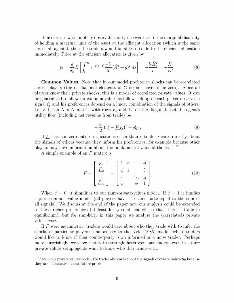
Common Values. Note that in our model preference shocks can be correlatedacross players (the off-diagonal elements of Σ do not have to be zero). Since allplayers know their private shocks, this is a model of correlated private values. It canbe generalized to allow for common values as follows. Suppose each player observes asignal ξit and his preferences depend on a linear combination of the signals of others.Let F be an N × N matrix with rows F i and 1’s on the diagonal. Let the agent’sutility flow (including net revenue from trade) be
− bi2
(xti − F iξt
)2+ qitpt, (9)
If F i has non-zero entries in positions other than i, trader i cares directly aboutthe signals of others because they inform his preferences, for example because otherplayers may have information about the fundamental value of the asset.12
A simple example of an F matrix is
F =
F 1
F 2...FN
=
1 φ · · · φ
φ 1...
.... . . φ
φ φ 1
(10)
When φ = 0, it simplifies to our pure-private-values model. If φ = 1 it impliesa pure common value model (all players have the same taste equal to the sum ofall signals). We discuss at the end of the paper how our analysis could be extendedto these richer preferences (at least for φ small enough so that there is trade inequilibrium), but for simplicity in this paper we analyze the (correlated) privatevalues case.
If F were asymmetric, traders would care about who they trade with to infer theshocks of particular players: analogously to the Kyle (1985) model, where traderswould like to know if their counterparty is an informed or a noise trader. Perhapsmore surprisingly, we show that with strategic heterogeneous traders, even in a pureprivate values setup agents want to know who they trade with.
12As in our private values model, the trader also cares about the signals of others indirectly becausethey are informative about future prices.
9

2.1 Mechanisms for trading.
We now turn to the determination of prices and trade flows. Existing papers withsymmetric rational traders model trading through a double uniform-price auction, asin Vayanos (1999) and Du and Zhu (2013), following the tradition of Kyle (1989).However, in our setting, since players are not symmetric, such a mechanism leadsto a complicated fixed point problem which involves filtering. For reasons that willbecome clear later, players would want to know not only the price but also informationabout who else is buying and selling. They would be making inferences about thedistribution of supply and demand, across players of different sizes, from the dynamicproperties of prices and through other means.
We instead propose an alternative trading mechanism in which players observe theflows currently being traded, with the goal of gaining the most insights about tradingdynamics in asymmetric markets in as simple a framework as possible. The benefit ofthis framework is that we obtain a separating equilibrium, in which dynamics dependonly on the vector of risk coefficients bi, and not the nature, correlation or varianceof the shocks. While the dynamics are simple, they are quite rich and capture manyof the phenomena that we set out to study.
The mechanism we propose is a uniform-price conditional double auction. We as-sume that players observe the flows of all other players, or can condition their demandfunctions on these flows. While we make this assumption out of necessity, there isevidence that market participants in practice spend a considerable amount of effortidentifying the sources of trades. For example, brokers call each other to find out whotraded, and some market-makers pay discount brokerages for the flow specifically fromretail investors. Moreover, recently NYSE began allowing orders from retail investorsto be marked as such through the Retail Liquidity Program (RLP). Finally, recentpopular books like Lewis “Flash Boys” or Patterson’s “Dark Pools” describe strategiesused by high-frequency traders to determine likely sources of trades. Therefore, wethink that the conditional auction model not only helps us with tractability but alsohelps us capture important real-life phenomena. Another interpretation of our modelis that it allows us to understand why traders care about the counterparty even ifthey do not believe that the counterparty has private information about fundamentalvalue.
Formally, our conditional double auction format is defined as:
Conditional Double-Auction. At each moment of time t, each player iannounces a supply-demand function
p = πi −∑j 6=i
πijqj
that gives the price at which the player is willing to trade, as a function of the sellingrates of all other players (with player i buying the net residual supply). The market
10
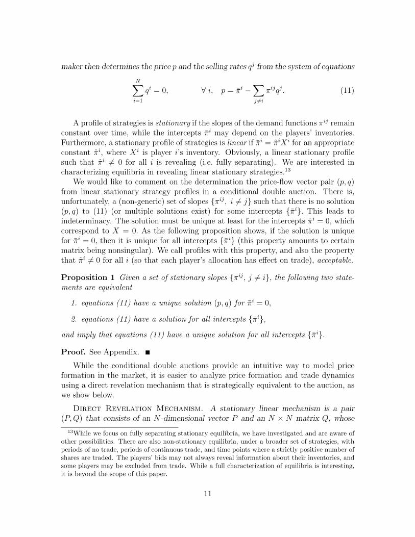
maker then determines the price p and the selling rates qj from the system of equations
N∑i=1
qi = 0, ∀ i, p = πi −∑j 6=i
πijqj. (11)
A profile of strategies is stationary if the slopes of the demand functions πij remainconstant over time, while the intercepts πi may depend on the players’ inventories.Furthermore, a stationary profile of strategies is linear if πi = πiX i for an appropriateconstant πi, where X i is player i’s inventory. Obviously, a linear stationary profilesuch that πi 6= 0 for all i is revealing (i.e. fully separating). We are interested incharacterizing equilibria in revealing linear stationary strategies.13
We would like to comment on the determination the price-flow vector pair (p, q)from linear stationary strategy profiles in a conditional double auction. There is,unfortunately, a (non-generic) set of slopes {πij, i 6= j} such that there is no solution(p, q) to (11) (or multiple solutions exist) for some intercepts {πi}. This leads toindeterminacy. The solution must be unique at least for the intercepts πi = 0, whichcorrespond to X = 0. As the following proposition shows, if the solution is uniquefor πi = 0, then it is unique for all intercepts {πi} (this property amounts to certainmatrix being nonsingular). We call profiles with this property, and also the propertythat πi 6= 0 for all i (so that each player’s allocation has effect on trade), acceptable.
Proposition 1 Given a set of stationary slopes {πij, j 6= i}, the following two state-ments are equivalent
1. equations (11) have a unique solution (p, q) for πi = 0,
2. equations (11) have a solution for all intercepts {πi},
and imply that equations (11) have a unique solution for all intercepts {πi}.
Proof. See Appendix.
While the conditional double auctions provide an intuitive way to model priceformation in the market, it is easier to analyze price formation and trade dynamicsusing a direct revelation mechanism that is strategically equivalent to the auction, aswe show below.
Direct Revelation Mechanism. A stationary linear mechanism is a pair(P,Q) that consists of an N -dimensional vector P and an N × N matrix Q, whose
13While we focus on fully separating stationary equilibria, we have investigated and are aware ofother possibilities. There are also non-stationary equilibria, under a broader set of strategies, withperiods of no trade, periods of continuous trade, and time points where a strictly positive number ofshares are traded. The players’ bids may not always reveal information about their inventories, andsome players may be excluded from trade. While a full characterization of equilibria is interesting,it is beyond the scope of this paper.
11
columns add up to 0. In this mechanism, at each moment of time t the marketmaker asks every trader to announce his inventory X i
t . The vector of announcementsdetermines the price pt = PXt and the vector of trading rates qt = QXt. We call themechanism truthtelling if telling the truth is an equilibrium of the mechanism whenannouncements are observable.14
Let us call a stationary linear mechanism (P,Q) acceptable if for any X in thenull space of Q (so that QX = 0), price PX = 0 only if X = 0. For an acceptablemechanism, there is a one-dimensional space of allocations X that result in no trade(i.e. it is the null space of Q) and all of these allocations result in different prices.
Proposition 2 The following statements about a mechanism (P,Q) are equivalent:
• it is acceptable;
• the matrix QP obtained by replacing the first (or any other) row of Q with thevector P is invertible; and
• if everybody tells the truth, the allocation X can be inferred by the outside ob-server from the price p and the vector of flows q.
Proof. See Appendix.
The last property implies that for acceptable mechanisms, the requirement thatannouncements are observable in the definition of a truthtelling mechanism can bereplaced with the requirement that the price and all trading flows are observable.That is, players can fully infer the inventories of others from the price and the tradingflows.
The following theorem provides a result about equivalence between acceptablemechanisms and (linear stationary) strategy profiles in a conditional double auction.15
Theorem 1 There is a one-to-one map between
• acceptable profiles of linear stationary strategies and
• acceptable mechanisms, such that for any nonzero allocation X that results inno trade, every element of X is nonzero
14That is, a truthtelling mechanism has to be ex-post incentive compatible.15The one-to-one map implies that mechanisms that are not acceptable do not generate dynam-
ics that correspond to any profile of a conditional double auction. Conversely, for a profile in aconditional double auction that is not acceptable, the map X → (p, q) is not well-defined.
12

that lead to the same map X → (p, q).Moreover, consider a profile {(πi, πij), j 6= i} and a corresponding mechanism
(P,Q). Then for each player i, for any allocation X−i of other players, player i canattain the same one-dimensional sets of price-trading flow pairs (p, q) by making areport in a mechanism or by submitting a supply-demand function in a strategy profileof a conditional double auction.
Proof. See Appendix.
An immediate corollary of this theorem is that, since each player has the samedegree of control over prices and flows in corresponding mechanism and profile ofa double auction, a profile of a double auction is an equilibrium if and only if thecorresponding mechanism is truth telling.
Corollary 1 If an acceptable profile of a conditional double auction is an equilibrium,then the corresponding direct revelation mechanism is truthtelling, and vice versa.
In all the equilibria that we construct below for every vector of reports of others,trader i can find a report that implies he does not trade (because his trade is linearlyincreasing in his report). For such equilibria ex-post incentive compatibility impliesthat (ex-post) individual rationality holds.
From now on we will focus on truth telling direct revelation mechanisms, as therepresentation in terms of P and Q provides a convenient direct map from the players’allocations to prices and flows.
3 Equilibrium Characterization.
We now derive equations that characterize trading dynamics under stationary linearequilibria in our model. We cover the case of N large players first. At the end wedescribe what happens when player N represents a continuum of players with totalrisk capacity of 1/bN , representing a competitive fringe.
Under mechanism (P,Q), on the equilibrium path the vector of trading flows isgiven by qt = QXt and the price is pt = PXt. If player i deviates and reports inventoryy +X i
t instead of X it , then the resulting price is PXt + piy and the vector of trading
flows is QXt +Qiy, where Qi is the ith column of Q, and pi is the ith element of P .Hence, from (5), the inventory vector follows
dXt = Σ dZt −QXt dt−Qiy dt. (12)
Under this law of motion, the value function f i(X) of player i must satisfy theHJB equation
rf i(X) = maxy
−bi
2(X i)2 + (PX + piy)(QiX + qiiy)− (13)
13

f ix(X)(QX +Qiy) +1
2tr [ΣΣTf ixx(X)],
where Qi is the i-th row of Q, qii is the i-th diagonal entry of Q, f ix is the gradientof f i and f ixx is the Hessian. In a truth-telling mechanism, y = 0 must solve themaximization problem in (13) for all inventory vectors X.
Since (13) is a quadratic optimization problem, the value function must be ofquadratic form f i(X) = XTAiX + ki, where Ai is a symmetric N ×N matrix and ki
is a constant. Then the HJB equation (13) becomes
r(XTAiX + ki) = maxy
−bi
2(X i)2 + (PX + piy)(QiX + qiiy) (14)
−2XTAi(QX +Qiy) + tr [ΣΣTAi].
Taking the first-order condition at y = 0, the HJB equation reduces to the follow-ing system of equations
piQi + qiiP = 2(AiQi)T , (15)
rAi + AiQ+QTAi =P TQi + (Qi)TP
2− bi
21ii and ki =
tr [ΣΣTAi]
r, (16)
where 1ii denotes the square N -by-N matrix that has 1 in the i-th diagonal positionand zeros everywhere else.
We call matrix Q stable if it has no eigenvalues with positive real parts. Stabilityimplies that the transversality condition E[e−rtX2
t ] → 0 holds on the equilibriumpath. The following proposition formally registers the fact that appropriate solutionsof equations (15) and (16) indeed lead to equilibria.
Proposition 3 Consider any solution (P,Q, ki, Ai, i = 1, . . . N) of the system (15)and (16) such that pi < 0 and qii ≥ 0 for all i = 1, . . . N, and the matrix Q is stable.Then, for all i if all other players tell the truth in mechanism (P,Q), it is betterto follow the truthtelling strategy than any other strategy that satisfies the no-Ponzicondition E[e−rtX2
t ]→ 0.16 That is, (P,Q) is a stationary linear equilibrium.
Proof. See Appendix.
The trading game has degenerate stationary equilibria, in which some or all of thetraders are excluded from the market (i.e. the matrix Q consists of zeros in severalrows and columns). Other degenerate equilibria involve a splitting of the market inwhich subsets of players trade among themselves, without trade across the subsets (sothat Q has zeros in some positions). We are interested primarily in non-degenerateequilibria (in which Q has no zeros, so all players trade with each other), and wouldlike to understand their properties such as the speed of trade, price momentum, andinefficiencies.
16If player i is allowed to violate the no-Ponzi condition, he can get infinite utility.
14

Equilibrium with a Competitive Fringe. We define a competitive fringe asa continuum of traders with a given finite risk capacity 1/bF . A group of m identicaltraders has risk capacity 1/bF if each trader has utility function of the form (6) withrisk coefficient mbF . Taking m→∞, we obtain a competitive fringe. We can includea competitive fringe into our model and, if so, we designate trader N as the fringe.17
The HJB equation for the total utility fN(X) of the fringe is given by the sameequation as the equation (16) for large traders.18 However, the first-order condi-tion differs from (15), since fringe members can no longer affect the price with theirindividual actions.
Proposition 4 If player N represents a competitive fringe, then prices and flowsmust satisfy the first-order condition
rP + PQ+ bF1N = 0, (17)
where 1N denotes a row vector with 1 in the N-th position and zeros everywhere else.
Proof. See Appendix.
If we right-multiply (17) by Xt it becomes rpt = −bFXFt + E[dpt
dt|Xt]. This op-
timality condition has a simple economic interpretation: since any member of thefringe has no price impact, he has to be indifferent between holding a marginal unitof inventory and selling it to buy back a moment later. Selling allows him to collectinterest flow on the cash; holding implies extra inventory cost and expected capitalgains (if price change in expectation).
Unfortunately, the system of (15) and (16) (together with (17) if player N rep-resents the fringe) in general cannot be solved in closed form. We can solve theequations numerically and provide several computed examples in Sections 4-6. Wealso present one useful (and surprisingly accurate) approximation of the solution.
We should note also that we do not necessarily view equations (15) and (16) asthe end goal, as there are many meaningful modifications of this set of equations. Wecan replace a single first-order condition (15) to model the behavior of a competitivefringe. Appendix A presents a model of risk-averse agents that care about bothfundamental and microstructure risk, and allows agents to have private informationabout fundamentals. In addition, if someone believes that our model may be too
17When analyzing a model with a fringe we restrict attention to equilibria that are symmetricwith respect to the fringe members, so that the fringe can be treated as one (as we mentioned above,our game has also degenerate equilibria in which some players are excluded altogether while otherstrade only within subgroups).
18For clarity, we maintain the assumption that all fringe members get identical shocks, but totalutility of the fringe is given by fN (X) even if individual fringe members get idiosyncratic shocksof bounded volatility driven by finitely many Brownian motions. Any misallocation among fringemembers gets traded to efficiency infinitely fast.
15

sophisticated to capture the behavior of various market participants, it is possibleto accommodate various forms of bounded rationality. For example, it is possible tostudy what happens when some or all of the players ignore price momentum thatoccurs as a result of asset allocation, or make incorrect assumptions about their priceimpact.
We can solve two special cases explicitly. First is the case when one large traderfaces a competitive fringe. This case is particularly useful because it illustrates mostof the important properties of trading in asymmetric markets, including the existenceof price momentum, the form and heterogeneity of price impact across players, andwelfare implications of market power. The next section describes trading in a marketwith a single large trader and competitive fringe. The second case we can solveexplicitly is when all players have identical risk coefficients - we present this solutionin Proposition 12.
4 Trading between a Large Player and a Fringe.
The following proposition characterizes in closed form equilibrium trading betweenone large player with risk capacity 1/bL and a competitive fringe with risk capacity1/bF .
Proposition 5 Consider a market with N = 2, in which player 1 is an individuallarge player and player 2 is a competitive fringe. Then in the unique nondegeneratelinear stationary equilibrium, equilibrium prices and the players’ trading rates arecharacterized by vectors
P = −1
r
bF
3bF + bL[bL, bL + 2bF
], Q =
r
2
[bL/bF −1−bL/bF 1
]. (18)
The welfare of the large trader and the fringe are characterized by matrices
AL =bF
2r(3bF + bL)
[−3bL −bL−bL bF
]and
AF =bF
2r (3bF + bL) (2bF + bL)
[(bL)2 −bLbF−bLbF −
((bL)2 + 5bLbF + 5(bF )2
) ]
Proof. See Appendix.
From this closed-form solution, we can analyze several salient properties of equilib-ria. We can divide properties into two groups: on and off equilibrium. On equilibriumproperties refer to what is seen by an independent observer - properties such as the
16

speed of trade and price momentum. Off-equilibrium we can analyze what happenswhen a single player deviates and changes the trading rate, i.e. we can analyze priceimpact.
Speed of Trade and Price Momentum. Let us discuss the properties of Pand Q. Matrix Q has two eigenvalues, 0 and
κ =r
2
bL + bF
bF(19)
with the corresponding eigenvectors being the efficient allocation and [1,−1]. That is,there is no trade if players are already at the efficient allocation, and any misallocationgets traded to efficiency at the rate (19). To understand why this is, we have to lookat player incentives by considering what would happen off equilibrium - we do thisin a bit. For now, let us observe that the speed of trade depends on how large trader1 is relative to the rest of the market. When trader 1 is small, as the risk capacity1/bL → 0, so the market gets closer to being fully competitive, trading speed (19)converges to infinity. It is interesting, however, that the trading speed here is alwaysbounded from below by r/2, a limit approached as the large player gets large, i.e.bL → 0.
The relationship between the speed of trade and market competitiveness is similarto the result of Vayanos (1999) that in symmetric markets the speed of trade increaseswith the number of players N, and is proportional to r(N − 2)/2. Here, when thelarge player is 1/N of market size, e.g. with 1/bL = 1 and 1/bF = N − 1, then (19)becomes equal to rN/2. That is, the speed of trade is on the order of the inverse ofplayer size, and it is slightly greater when the player faces a competitive market thanplayers of equal market power. The property that the speed of trade increases asthe market power of individual players falls extends to asymmetric markets that weconsider in the next section, with the new result that there may be different tradingspeeds in different market segments (i.e. matrix Q has several positive eigenvalues).
The price is first best whenever players are at an efficient allocation X, i.e. in thatcase PX = PX, where
P = −1
r
bLbF
bF + bL[1, 1]
is the first-best pricing vector. However, since P 6= P , price differs from first bestwhenever players are not at an efficient allocation. The immediate implication of thisis price momentum: in the absence of further inventory shocks, price converges to thefirst-best price at rate given by (19) as players trade to the efficient allocation. Withshocks, this is the expected price path.
The direction of price momentum is connected with the property that the price isskewed away from first best in favor of the large players. For example, at allocationX0 = [1,−1] the price is
p0 =1
r
2(bF )2
3bF + bL> 0.
17

That is, the large player starts selling at a positive price, while the first-best priceis 0.19 The sales of the large player produce a downward price momentum, in thisexample directed from p0 to 0. Conversely, when the large player is buying, theprice has an upward momentum. In contrast, in the symmetric-trader environmentof Vayanos (1999), there is no price momentum: the price immediately adjusts tofirst best following any shock. In general, as we explain in the next section, pricemomentum is driven by the unequal market power of current buyers and sellers. Theside with greater market power gets a temporary price advantage.
Price Impact. With our trading model, we can study how a given sequenceof trades affects the price. Effectively, we provide a game-theoretic way of derivingparameters of a model such as that of Almgren and Chriss (2001). It is also a result,rather than an assumption, that price impact of the large player takes the form givenby (1) when he is trading against a fringe.20 In general, however, our model impliesprice impact of a form that is more general than (1). Trades also have a transientprice impact, which has an empirical counterpart (see discussion in the next section).
We should emphasize that the study of price impact is essentially an off-equilibriumexercise. On equilibrium, a player has a uniquely optimal trading strategy. In prin-ciple, however, a player can choose to trade in any way he/she desires. Given anarbitrary set of trades, the market responds by forming incorrect beliefs about theplayer’s inventory. The price that the trader receives is a function of market beliefs,which are formed based on the trading speed. To solve for price impact followinga given path of sales by the large player qLs , s ∈ [0, t], we have to calculate marketbeliefs following these sales, i.e. infer the shocks of the large player that would haveresulted in this path of trades. The following proposition provides the form of thelarge player’s price impact in the model with a single large player and the fringe.
Proposition 6 The price impact of the large trader takes the form (1), where
Λ =bF
r, I =
Λ
r + κ, p0 = −ΛXF
0 , and σ = Π |ΣF |, (20)
where κ given by (19) is the speed of trade and ΣF represents the last row of Σ. Givena sequence of sales qLs , s ∈ [0, t], by the large trader, the fringe forms the belief about
19The deviation of the price from first best depends on the market power of the large trader.Suppose bF = 1, so that the marginal value of a unit to the fringe at allocation X = [1,−1] is 1/r.The actual price is less than this: it can get as high as 2/(3r) when bL → 0 (i.e. the large player hastremendous market power) but it approaches first best when the market power of the large playerdiminishes (i.e. as bL →∞).
20In the broader interpretation that pt is the deviation (due to microstructure forces) of the actualprice pt from the fundamental value, the volatility of the actual price pt would be greater than thatgiven by Proposition 10 due to fundamental shocks. Thus, representation (20) captures only themicrostructure shocks.
18

the large trader’s inventory to be
XLt =
bF
bL
(2
rqLt +XF
t
). (21)
Proof. The volatility of inventory shocks to the fringe is |ΣF |, so we can express
XFt = XF
0 + |ΣF | zt +
∫ t
0
qLs ds, (22)
where z is a Brownian motion. Now, given this allocation of the fringe, the relation-ship between the allocation of the large player and the selling rate, from the first rowof Q, is
qLt =r
2
(bL
bFXLt −XF
t
).
Then from the selling rate qLt , the fringe infers that XLt is given by (21).
Now, the price is given by PX, where (XLt , X
Ft ) is given by (21) and (22). There-
fore,
pt = −1
r
bF
3bF + bL
(bF(
2
rqLt +XF
t
)+ (bL + 2bF )XF
t
)=
−bF
r
(XF
0 + |ΣF | zt +
∫ t
0
qLs ds
)︸ ︷︷ ︸
XFt
−1
r
2bF
r
1
3 + bL/bFqLt .
This implies (20).
Proposition 6 confirms the intuitive guess that the permanent price impact Λ oflarge player’s trades (i.e. Kyle’s lambda) is proportional to the risk capacity of thefringe. On the other hand, the instantaneous price impact I depends also on therisk capacity of the large player relative to the fringe. A player of larger risk capacitytrades more slowly to minimize price impact, hence any selling rate qLt signals a largerinventory XL
t of the large player, according to (21). Hence, as the speed of trade κslows down, the price impact rises.
Large risk capacity or “patience” gives the large player market power to obtainbetter prices by selling slowly, but the expectations of the fringe of this behaviorraise the instantaneous price impact of the large player. This creates illiquidity in themarket, which is detrimental to the large player. Thus, “market power” bites backby reducing liquidity. There is ample anecdotal evidence that large traders try tohide information about their desire to buy or sell, e.g. by splitting orders into smallportions or waiting for the flow to trade against. In practice, therefore, to some extentlarge traders are able to hide their flow behind that of small retail investors, althoughother market participants, especially the high-frequency traders, seek to identify largetraders - see Patterson (2012).
19

Our model of trade presents an extreme benchmark in which the entire marketknows immediately when a large player is trading, and the price reacts accordingly.In this case, is market power beneficial to have? With transparency and rationalexpectations, the cost of market power is illiquidity - the large player is forced totrade slowly, even though he can take advantage of the current price in the short run.We can ask several questions to explore market power. Would several small playersbenefit by merging into a single large unit to coordinate trades? If the large playercould commit to a rate of trade in order to affect the expectations of the fringe andthe price impact, would the optimal rate be faster or slower than the equilibrium one?We address these and other questions next.
4.1 Market Power and Welfare.
Our general conclusion, which is somewhat counterintuitive, is that in transparentmarkets market power is detrimental. That is the cost of illiquidity that goes withmarket power outweighs the ability to control the price by trading slowly. We illus-trate this message via a sequence of three results, which we informally call “fractions”as they hold when the large player has less than 1/2, 1/3 and 1/4 of market risk ca-pacity, respectively.
First, we address the question of mergers. Suppose that in a fully competitivemarket a portion of the fringe merges to form a single large player in order to coordi-nate trades - would their welfare improve? To keep the experiment clean, we assumethat the fringe members who merge have identical shocks. Before the merger, thesefringe members trade in the same direction without taking into account price impact,i.e. the effect of their trades on the price that everybody else is facing.21 As a result,the price adjusts immediately to first best, and fringe members trade to efficiencyinstantaneously at that price. After the merger, the price adjusts gradually to firstbest, i.e. the newly formed large player trades at prices better than the first-bestprice, but slowly.
Proposition 7 In a fully competitive market, suppose that a mass of agents facingidentical inventory shocks, and with risk capacity less than 1/2 of the market, mergeto form a single large player. Then for any distribution of shocks, the total welfare ofthe merging players falls relative to the level before merger.
Proof. See Appendix.
Next, we observe that the price impact of the large player is connected with theequilibrium trading rate κ. What would happen if the large player could commit toany trading rate and the price impact is determined from the first-order condition
21The phenomenon in which agents to not take into account the effect that their trades have onthe price that other agents are facing is sometimes referred to as the “firesale externality.”
20
(17) given that rate? What is the optimal selling rate, and is it slower or faster thanthe equilibrium trading rate given by (19)?
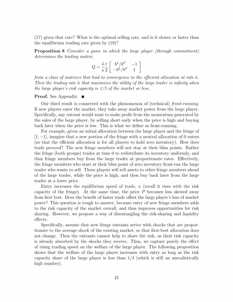
Proposition 8 Consider a game in which the large player (through commitment)determines the trading matrix
Q =κ
κ
r
2
[bL/bF −1−bL/bF 1
]from a class of matrices that lead to convergence to the efficient allocation at rate κ.Then the trading rate κ that maximizes the utility of the large trader is infinity whenthe large player’s risk capacity is 1/3 of the market or less.
Proof. See Appendix.
Our third result is connected with the phenomenon of (technical) front-running.If new players enter the market, they take away market power from the large player.Specifically, any entrant would want to make profit from the momentum generated bythe sales of the large player, by selling short early when the price is high and buyingback later when the price is low. This is what we define as front-running.
For example, given an initial allocation between the large player and the fringe of[1,−1], imagine that a new portion of the fringe with a neutral allocation of 0 enters(so that the efficient allocation is for all players to hold zero inventory). How doestrade proceed? The new fringe members will not stay at their bliss points. Ratherthe fringe (both groups) trades at time 0 to redistribute its inventory uniformly, andthen fringe members buy from the large trader at proportionate rates. Effectively,the fringe members who start at their bliss point of zero inventory front-run the largetrader who wants to sell. These players will sell assets to other fringe members aheadof the large trader, while the price is high, and then buy back later from the largetrader at a lower price.
Entry increases the equilibrium speed of trade, κ (recall it rises with the riskcapacity of the fringe). At the same time, the price P becomes less skewed awayfrom first best. Does the benefit of faster trade offset the large player’s loss of marketpower? This question is tough to answer, because entry of new fringe members addsto the risk capacity of the market overall, and thus improves opportunities for risksharing. However, we propose a way of disentangling the risk-sharing and liquidityeffects.
Specifically, assume that new fringe entrants arrive with shocks that are propor-tionate to the average shock of the existing market, so that first-best allocation doesnot change. Then the entrants cannot help to share the risk, as their risk capacityis already absorbed by the shocks they receive. Thus, we capture purely the effectof rising trading speed on the welfare of the large player. The following propositionshows that the welfare of the large player increases with entry as long as the riskcapacity share of the large player is less than 1/4 (which is still an unrealisticallyhigh number).
21

Proposition 9 Suppose that the risk capacity share of the large player is less than1/4. If new fringe members enter without adding risk capacity (i.e. with shocks suchthat first best allocation does not change) then the welfare of the large player goes up.
Proof. See Appendix.
We finish this section with a general observation. With transparency about thesource of flow, the market anticipates large players to split their trades into smallportions. As a result, the price impact of even small orders becomes large, whichharms the welfare of large players, even though by exercising their market power theyare able to extract a better price. As we show in Section 5, with a heterogeneousmarket of N strategic players, larger traders trade more slowly and have a greaterprice impact. It is not surprising then that in practice, large traders want to hidetheir flow behind that of small traders, in order to take advantage of the privateinformation about their supply or demand for as long as possible.
5 Equilibria with N Large Traders.
In this section we describe the properties of equilibria in a market with N largetraders. We follow the same classification of results as in Section 4, by distinguishingon and off-equilibrium phenomena.
On equilibrium, the speed of trade depends on the overall competitiveness ofthe market and the market power of individual players. Small players trade faster,and misallocations among small players get traded to efficiency faster than thoseamong large players, as captured by the eigenvector decomposition of Q. Equilibriumprice deviates from first best, depending on the allocation among players and theirsize/market power. While first-best price depends only on total inventory, i.e. it isequally sensitive to allocations of all players, equilibrium price is more sensitive tothe inventories of small players than those of large players. That is, as the marketconverges towards the efficient allocation, market price is skewed in favor of the largeplayers. In equilibrium price drifts to first best. This price momentum depends on therelative market power of buyers and sellers. For example, if there is a small numberof large buyers and many small sellers at a given moment of time, the price drifts up.
Off equilibrium, trades of an individual player have permanent price impact (i.e.Kyle’s λ), which depends on the risk capacity of the rest of the market, and in-stantaneous impact, as in the model with a single large player and a fringe. Theinstantaneous impact, the sensitivity of price to flow, is different for players of differ-ent size. Instantaneous impact is greater for larger players, as they trade more slowlyand retain a greater portion of their inventory for longer. In addition, trades havetransient impact: i.e. price reaction to total sales that decays over time. Transientimpact exists because players do not absorb flow proportionately to risk capacity and
22

so, when sales by a single player stop, trade among other players continues, affectingthe price.
To sum up, while most properties of equilibria are apparent already in the closed-form solution with a single large player and a fringe, we observe a more completepicture and several new phenomena in the general model. In general, the speed oftrade varies by the competitiveness of a market segment. Also the general model illus-trates in greater depth how price momentum depends on the relative competitivenessof buyers and sellers. Moreover, instantaneous price impact depends on player iden-tity, providing a rationale for why the knowledge of the origin of trade flow matters agreat deal to sophisticated market participants in practice. Finally, the general modelgives rise to the transient price impact: while this effect is absent from Almgren andChriss (2001), it exists empirically.
Unfortunately, in general our model does not have exact analytical solutions.Hence, we illustrate these results, first, using computed examples and, second, ana-lytically using an approximation of true solutions that is valid near the symmetriccase. That approximate solution provides explanation and analytical basis for thepatterns we observe in the numerical examples.
5.1 Equilibrium Trade.
We start by discussing trade on the equilibrium path, from the perspective of an out-side observer. Players trade towards the efficient allocation with speeds that dependon their size. Price momentum exists, and depends on the relative risk capacity ofbuyers and sellers.
Example. Let us start with a simple example which captures broadly the proper-ties we observed from exploring numerically solutions to many examples. We discusseconomic intuition here, and at the end of this section we provide analytical resultsthat affirm these properties.
Consider a game with five traders, whose holding cost coefficients are
[b1, b2, b3, b4, b5] = [1, 1.5, 2, 2.5, 3],
and the discount rate is normalized to r = 1. Solving the equilibrium conditionsnumerically, we get that any allocation X is priced by vector
P = [−.254,−.329,−.387,−.435,−.476],
and the rates of trading flows are given by matrix
Q =
0.630 −0.244 −0.319 −0.389 −0.455−0.163 0.965 −0.326 −0.401 −0.473−0.160 −0.244 1.289 −0.405 −0.481−0.156 −0.241 −0.324 1.598 −0.483−0.152 −0.236 −0.320 −0.403 1.892
.
23
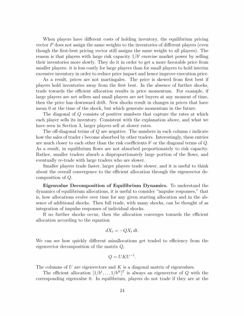
When players have different costs of holding inventory, the equilibrium pricingvector P does not assign the same weights to the inventories of different players (eventhough the first-best pricing vector still assigns the same weight to all players). Thereason is that players with large risk capacity 1/bi exercise market power by sellingtheir inventories more slowly. They do it in order to get a more favorable price fromsmaller players: it is less costly for large players than for small players to hold interimexcessive inventory in order to reduce price impact and hence improve execution price.
As a result, prices are not martingales. The price is skewed from first best ifplayers hold inventories away from the first best. In the absence of further shocks,trade towards the efficient allocation results in price momentum. For example, iflarge players are net sellers and small players are net buyers at any moment of time,then the price has downward drift. New shocks result in changes in prices that havemean 0 at the time of the shock, but which generate momentum in the future.
The diagonal of Q consists of positive numbers that capture the rates at whicheach player sells its inventory. Consistent with the explanation above, and what wehave seen in Section 3, larger players sell at slower rates.
The off-diagonal terms of Q are negative. The numbers in each column i indicatehow the sales of trader i become absorbed by other traders. Interestingly, these entriesare much closer to each other than the risk coefficients bi or the diagonal terms of Q.As a result, in equilibrium flows are not absorbed proportionately to risk capacity.Rather, smaller traders absorb a disproportionately large portion of the flows, andeventually re-trade with large traders who are slower.
Smaller players trade faster, larger players trade slower, and it is useful to thinkabout the overall convergence to the efficient allocation through the eigenvector de-composition of Q.
Eigenvalue Decomposition of Equilibrium Dynamics. To understand thedynamics of equilibrium allocations, it is useful to consider “impulse responses,” thatis, how allocations evolve over time for any given starting allocation and in the ab-sence of additional shocks. Then full trade, with many shocks, can be thought of asintegration of impulse responses of individual shocks.
If no further shocks occur, then the allocation converges towards the efficientallocation according to the equation
dXt = −QXt dt.
We can see how quickly different misallocations get traded to efficiency from theeigenvector decomposition of the matrix Q,
Q = UKU−1.
The columns of U are eigenvectors and K is a diagonal matrix of eigenvalues.The efficient allocation [1/b1, . . . 1/bN ]T is always an eigenvector of Q with the
corresponding eigenvalue 0. In equilibrium, players do not trade if they are at the
24

efficient allocation: if they traded then at least one player would be worse off than ifhe had not traded at all. If matrix Q has rank N − 1 (a requirement for the mech-anism (P,Q) to be acceptable), then the remaining eigenvectors of Q have nonzeroeigenvalues. Market clearing implies that the coefficients of those eigenvectors add upto 0, i.e. eigenvectors are misallocations away from efficiency, and the correspondingeigenvalues are the rates at which those misallocations get traded away. If in equilib-rium players eventually trade to efficiency, then the remaining N − 1 eigenvalues ofQ must be positive.
The following lemma transforms the equilibrium conditions into a simpler formusing the eigenvector decomposition of Q.
Lemma 2 Consider a mechanism characterized by a vector P and a trading matrixQ that has only real eigenvectors, with decomposition Q = UKU−1. Then the HJBequations (16) that determine the value functions of the players under truthtelling areequivalent to Ai = UTAi U, i = 1 . . . N, where the coefficients of Ai are given by
aijk =−biuijuik + (PU j)uikκk + (PUk)uijκj
2(r + κk + κj), (23)
and κk is the k-th diagonal element of K.Given (23), the first-order conditions (15) can be written as
uik
(bi + κk(r + κk)
PU 1r+κk+K
(U−1)i
U i Kr+κk+K
(U−1)i
)= −(r + κk)PU
k. (24)
Proof. See Appendix.
Equations (23) provide a convenient direct formula to compute the players’ valuefunctions from the pair (P,Q). Otherwise, to obtain the matrices Ai from (16), onehas to solve a more complicated system of equations, or obtain Ai via an iterativeprocedure. Equation system (24) is useful because it expresses the equilibrium con-ditions purely in terms of the vector P and the eigenvector decomposition UKU−1 ofQ, i.e. it provides a simpler system of equations than the system (15) and (16).
Example continued. Returning to our numerical example, the eigenvector de-composition of Q is given by
U =
1 1 .218 .118 .081.666 −.530 .782 .214 .123.5 −.221 −.619 .668 .213.4 −.143 −.234 −.748 .583.333 −.106 −.147 −.252 −1
, diag K= [0, .93, 1.38, 1.82, 2.24].
(25)
25
Note the sign pattern in the eigenvectors: they break the market into two sidesaccording to risk capacity, with one side of the market selling and the other, buying.The eigenvectors, the columns of Q, are determined only up to a constant. Wenormalized eigenvectors 2 through N so that one unit in total is misallocated betweenlarge sellers and small buyers. Misallocations among the smallest players get tradedaway faster than those among the largest players in the market: for example, thesecond eigenvector represents the largest trader having excess inventory while thelast vector represents the smallest trader having excess inventory; the latter is tradedat more than twice the speed of the former.
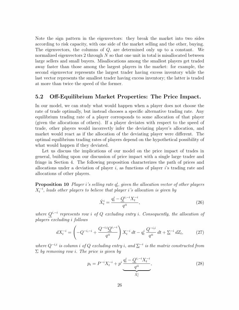
5.2 Off-Equilibrium Market Properties: The Price Impact.
In our model, we can study what would happen when a player does not choose therate of trade optimally, but instead chooses a specific alternative trading rate. Anyequilibrium trading rate of a player corresponds to some allocation of that player(given the allocations of others). If a player deviates with respect to the speed oftrade, other players would incorrectly infer the deviating player’s allocation, andmarket would react as if the allocation of the deviating player were different. Theoptimal equilibrium trading rates of players depend on the hypothetical possibility ofwhat would happen if they deviated.
Let us discuss the implications of our model on the price impact of trades ingeneral, building upon our discussion of price impact with a single large trader andfringe in Section 4. The following proposition characterizes the path of prices andallocations under a deviation of player i, as functions of player i’s trading rate andallocations of other players.
Proposition 10 Player i’s selling rate qit, given the allocation vector of other playersX−it , leads other players to believe that player i’s allocation is given by
X it =
qit −Qi,−iX−itqii
, (26)
where Qi,−i represents row i of Q excluding entry i. Consequently, the allocation ofplayers excluding i follows
dX−it =
(−Q−i,−i +
Q−i,iQi,−i
qii
)X−it dt− qit
Q−i,i
qiidt+ Σ−i dZt, (27)
where Q−i,i is column i of Q excluding entry i, and Σ−i is the matrix constructed fromΣ by removing row i. The price is given by
pt = P−iX−it + piqit −Qi,−iX−it
qii︸ ︷︷ ︸Xit
, (28)
26
where P−i represents vector P excluding entry i.
Proof. Notice that if player i acted as if he had allocation X it , then the selling rate
of player i would be given by
qit = qiiX it +Qi,−iX−it .
Solving for X it given qit, we find (26). Plugging in the allocation X i
t of the typethat player i is imitating into the law of motion of Xt and into the price formationequation, we obtain (27) and (28).
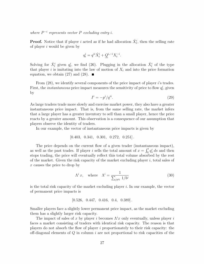
From (28), we identify several components of the price impact of player i’s trades.First, the instantaneous price impact measures the sensitivity of price to flow qit, givenby
I i = −pi/qii. (29)
As large traders trade more slowly and exercise market power, they also have a greaterinstantaneous price impact. That is, from the same selling rate, the market infersthat a large player has a greater inventory to sell than a small player, hence the pricereacts by a greater amount. This observation is a consequence of our assumption thatplayers observe the identity of traders.
In our example, the vector of instantaneous price impacts is given by
[0.403, 0.341, 0.301, 0.272, 0.251] .
The price depends on the current flow of a given trader (instantaneous impact),as well as the past trades. If player i sells the total amount of x =
∫ t0qis ds and then
stops trading, the price will eventually reflect this total volume absorbed by the restof the market. Given the risk capacity of the market excluding player i, total sales ofx causes the price to drop by
Λi x, where Λi =1∑
j 6=i 1/bj(30)
is the total risk capacity of the market excluding player i. In our example, the vectorof permanent price impacts is
[0.526, 0.447, 0.416, 0.4, 0.389] .
Smaller players face a slightly lower permanent price impact, as the market excludingthem has a slightly larger risk capacity.
The impact of sales of x by player i becomes Λix only eventually, unless player ifaces a market consisting of traders with identical risk capacity. The reason is thatplayers do not absorb the flow of player i proportionately to their risk capacity: theoff-diagonal elements of Q in column i are not proportional to risk capacities of the
27

players. Smaller players absorb a disproportionate share of flow, and if player i stopstrading, other players continue trading among themselves. Since smaller players alsohave a greater price impact, their disproportionate absorption of player i’s tradescauses the price to overshoot the permanent price impact level. Hence, trades have atransient price impact.
Denote by T i + Λi the sensitivity of price to sales of player i, when the sales ofx by player i occur over a short interval of time [0, t], as t → 0. Then the vector oftransient price impacts T i in our example is
[0.020, 0.055, 0.054, 0.045, 0.034] ,
and these coefficients can be computed from the following lemma.
Lemma 3 If sales of x by player i occur over a small interval of time [0, t] and thenstop, then as t→ 0, total (permanent and transient) impact of trades is given by
(T i + Λi)x =P + I iQi
qiiQix. (31)
Proof. The sales of x are initially absorbed by players j 6= i according to X−i0+−X−i0 =−Q−i,i/qii x. Thus, from (28), the price immediately after sales stop is given by
p0+ = p0−P−iQ−i,i
qiix+ pi
Qi,−i
qiiQ−i,i
qiix︸ ︷︷ ︸
−P+IiQi
qiiQix
.
Hence, the impact of sales is given by (31).
To get a better sense for price impact, suppose that in our example player 3(with risk capacity of b3 = 2) sells at rate q3
t = 1 over the time interval [0, 0.5] andthen stops trading. Assume that other players do not receive any shocks. Then,integrating equations (27) and (28), we get the path of prices shown in Figure 1.To recap, transient impact (which is quantitatively small here) exists because salesof player 3 are not absorbed by others proportionately to risk-capacity, hence afterplayer 3 stops selling, other players continue trading among each other.
The term “transient impact” is also used to capture the empirical pattern thatthe price, following an interval of sales, overshoots and retracts a bit after sales cease.
28

time0 0.2 0.4 0.6 0.8 1 1.2 1.4 1.6 1.8 2
pric
e im
pact
-0.5
-0.4
-0.3
-0.2
-0.1
0
permanent
transient + permanent
total
instantaneous
Figure 1: The decomposition of price impact.
5.3 Optimal Trading without Transient Price Impact.
Optimal trading with only instantaneous and permanent price impact has a simplecharacterization, which we derive here. This case is of special interest, because we canuse it to quickly derive equilibrium in the case of a symmetric market, where play-ers have no transient price impact, and approximate equilibria in nearly symmetricmarkets, where transient impact is second order.
In general, this case leads to a simple approximately optimal rule for trading,which is helpful because (1) transient impact in our model is small and (2) it iscomplex, since the rates of decay of transient impact depend on the eigenvalues oftrading dynamics among players other than player i.
Proposition 11 Suppose player i’s trades have only instantaneous and permanentprice impact characterized by coefficients I i and Λi. Then, in order for player i’sstrategy to be optimal, the following condition has to hold
r(pt − I iqit) = −biX it + Λiqit + Et
[d(pt − I iqit)/dt
]. (32)
Equation (32) generalizes condition (17) of Proposition 4 that characterizes opti-mal trading of a fringe. Indeed, fringe members act as if their trades have no priceimpact at all (instantaneous or permanent). In equation (32), pt−I iqit is the marginal
29

revenue of player i from an extra unit sold. Thus, unlike (17), which can be writtenas
rpt = −biX it + Et [dpt/dt] ,
equation (32) is a condition on the level and rate of change of not the price, but rathermarginal revenue. In vector form, equation (32) can be written as
(P − I iQi)(rI −Q) = −bi1i + ΛiQi. (33)
Notice, in particular, that if player i trades according to (32), player i does notignore the equilibrium-path price momentum. Rather, this condition requires a highlevel of sophistication - player i recognizes who the buyers and the sellers in themarket are, and how their behavior pushes the price. Player i is only biased aboutthe hypothetical scenario of what would happen if he traded at an off-equilibriumrate, potentially underestimating the impact on price a little bit. When transientprice impact exists, equation (32) leads to a slight bias to more aggressive tradingrelative to a fully rational trader.22
Proof. Consider the optimal strategy qit and a deviation qit+yt. The deviation resultsin the allocation
X it = X i
t −∫ t
0
ys ds.
If pt is the price process for the strategy qit, then the price after a deviation, givenonly the instantaneous and permanent price impacts, becomes
pt − Λi
∫ t
0
ys ds− I iyt = pt + Λi(X it −X i
t)− I iyt.
Denote by vt the player’s value function under the strategy qit, and conjecture thefollowing quadratic form
a(X it −X i
t)2 + bt(X
it −X i
t) + vt (34)
for the value function after the deviation, where a is an appropriate constant and btdepends on the stochastic environment of the price process. The HJB equation is
r(a(X i
t −X it)
2 + bt(Xit −X i
t) + vt
)= max
yt−b
i(X it −X i
t +X it)
2
2︸ ︷︷ ︸−bi(Xi
t)2/2, payoff flow
+
(pt + Λi(X it −X i
t)− I iyt)(qit + yt)− 2yta(X it −X i
t)− btyt +Et[dbt]
dt(X i
t −X it) +
Et[dvt]
dt.
22In general, we believe that there can be huge insights from exploring the dynamics of this modelwith players of various levels of sophistication. Equations such as (32) can be used to formulatetrading rules for particular subgroups of players.
30

If we solve this equation with yt = 0, then we obtain a lower bound on player i’svalue function after a deviation (since yt = 0 is not necessarily optimal following adeviation). Matching coefficients on (X i
t−X it)
2 and X it−X i
t , we obtain a lower boundif
ra = −bi
2and rbt = −biX i
t + Λiqit +Et[dbt]
dt(35)
(notice that the coefficient on the constant matches automatically from the defini-tion of vt as the value function). Given this bound, in order for player i to find itunattractive to deviate when X i
t = X it , the first-order condition with respect to yt
must hold at yt = 0, i.e. we must have
bt = pt − I iqit. (36)
Combining this with the condition for coefficient bt we obtain (32).23
5.4 N Traders with Symmetric Risk Capacities.
Let us use Proposition 11 to characterize dynamics in a market with N traders ofidentical risk capacities.
Proposition 12 Consider a market of N traders with identical risk coefficients b.Then the equilibrium price and trading dynamics in the unique non-degenerate sym-metric equilibrium are characterized by the pair
P = − b
Nr1 and Q =
N − 2
2r︸ ︷︷ ︸
κ
(I − S/N), (37)
where 1 is a row vector of ones and S is an N × N matrix of ones. That is, theallocation converges towards efficiency at the exponential rate κ.
The players’ welfare is characterized by the matrices Ai with entries
aiii = −rb2
3N − 2
N2, aiij = −rb
2
N − 2
N2and aijk =
rb
2
N − 2
(N − 1)N2(38)
23We only showed that condition (32) is necessary. For sufficiency, we can show that the actualvalue function also takes the form (34). Indeed, the first-order condition for yt in the HJB equation,given (36), is
yt =(Λi − 2a)(Xi
t −Xit)
2Ii.
Plugging this into the HJB equation and matching coefficients, we obtain
ra = −bi
2+
(Λi − 2a)2
4Ii
and the same equation for bt as in (35). That is, the true value function and the upper bound weused have the same slope at Xi
t = Xit (obviously, if the first-order condition with respect to yt is to
hold) but the true function is less concave, i.e. a is higher.
31

for j, k 6= i.
Proof. From symmetry, matrix Q must be of the form κ(I − S/N) and vector Pmust have identical coefficients p. Player i’s trades have no transient impact (sinceflow of any player is absorbed efficiently) so price impact of player i is characterizedby (we use (31) to get Λi)
I i = − p
qii= − pN
(N − 1)κand Λi = − p
qiiQiQi
qii= − pN
N − 1.
We now use optimal trading condition (32). If∑
j Xj = Nx, then price is pt =
Npx. Since expected change in total supply is 0, Et[dpt] = 0. The allocations convergeto the efficiency at rate κ, i.e. qit = κ(X i
t − x), and player’s trading rates also decayat expected rate κ, i.e. Et[dq
it] = −κ2(X i
t − x). Hence, (32) becomes
r(pNx− I iκ(X it − x)) = −bX i
t + Λiκ(X it − x) + I iκ2(X i
t − x). (39)
Matching coefficients in (32), we obtain
x : rp(N − 2) = 2pκ ⇒ κ =N − 2
2r
X it : (r + 2κ)
pN
N − 1= −b ⇒ p = − b
Nr.
In the Appendix we provide an alternative proof, using the system of equilibriumequations (15) and (16) directly, and derive the players’ value functions.
Intuitively, the price vector P must have all the same elements from symmetry,and must correspond to the first best price (otherwise, if players are at the efficientallocation already, they would still want to trade). Since inventory shocks have zeromean, it follows that prices are martingales in equilibrium of the symmetric bench-mark. Off-equilibrium, trades have instantaneous and permanent price impact. Asa result, players take time to trade to the efficient allocation, and so the equilibriumis inefficient (even though prices are first-best on the equilibrium path).24 Not sur-prisingly, the speed of trade is increasing in the number of players in the market,suggesting that market power could be bad for efficiency.25
24As we mentioned before, an analogous result has already been shown in a slightly differentcontext in Vayanos (1999).
25The full effect is more subtle though. If traders merged in pairs (so that the market would movefrom N to N/2 traders) and the merged traders shared their inventories efficiently, for a symmetricΣ the overall welfare would actually remain unchanged. Such a merger would result in two oppositeeffects that exactly cancel each other out in the symmetric model: the market would converge toefficiency at a slower rate, which hurts efficiency, but the merged players would share their shocksmore efficiently, which helps welfare.
32

It may seem surprising at first that value function matrices Ai have positive coef-ficients everywhere outside column and row i (see equation (38)). The reason is that,while players experience disutility from shocks to their own allocations - which theyhave to hold or pay other traders to offload - players actually earn utility by takingexcess inventory off of other players. Therefore, in equilibrium players who help otherplayers trade - liquidity providers - may have positive expected utility.
5.5 Approximation near Symmetric Risk Capacities.
While in general we cannot characterize equilibrium in closed form, we can approxi-mate equilibria, up to terms of order ε2, near symmetric risk coefficients, perturbedby terms of order ε. As we show in a bit, the approximate formulas we obtain areextremely useful. First, in practice the approximate formulas generate answers thatare quite precise even in cases where risk coefficients bi are not nearly symmetric.Second, we can use the approximate formulas to illustrate analytically the importanteconomic properties of asymmetric markets.
It is possible to derive an approximation of equilibria near the symmetric caseusing formulas (15) and (16) for the perturbation of risk coefficients
b (1 + ε), (40)
directly by keeping only terms of order |ε|. In (40), 1 is a row vector of ones andε is a small vector whose coefficients add up to 0.
Proposition 13 Consider the perturbation of symmetric risk coefficients (40). Then,equilibrium equations hold, up to terms of order |ε|2, for the pair (P , Q) given by
P = P (I + xPDε), xP =3N − 4
N(N − 1)and Q = Q(I +Dε), (41)
where P and Q are the pair that solves the symmetric case (37), and Dε is a diagonalmatrix with vector ε on the diagonal. The transient price impact is of order |ε|2.
Recall that post-multiplication by a diagonal matrix I +Dε in (41) results in themultiplication of the columns of the preceding matrix (in this case Q) by the entriesof the diagonal elements.
We take a shortcut to prove Proposition 13, using the property that transient priceimpacts are of order |ε|2 near the symmetric case.26 Then the the characterization ofProposition 11 applies. As a result, we bypass the algebra that involves value functionmatrices Ai, and focus only on equations that contain P and Q.
26Transient impact is of second-order because absorption of sales by any player is up to order εproportionate to risk capacities and price is, up to order ε, first best. Taking these effects together,transient price impact is of second order. See the proof of Proposition 13.
33

Proof. We have from (29) and (30), using expressions for P , Q in (41),
I i =b/r
(N − 1)κ(1 + (xP − 1)εi) +O(|ε|2), (42)
and Λi =b/r
N − 1
(1− εi
N − 1
)+O(|ε|2).
Furthermore, (31) yields
T i + Λi =
(P+IiQi)Qi︷ ︸︸ ︷
bκ
rN
(1 +
N − 2
N − 1εi)
+O(|ε|2)
N−1
Nκ(1 + εi
)+O(|ε|2)︸ ︷︷ ︸
qii
= Λi +O(|ε|2).
Hence, transient impact is of order |ε|2, and we can use equations (33) to characterize(the approximate) equilibrium. In matrix form, these equations can be written as
DΛQ = DB + (1T P −DIQ)(rI + Q), (43)
where DΛ, DI and DB are diagonal matrices of permanent and instantaneous priceimpacts, and the players’ risk coefficients, respectively. Plugging in (41), we obtain27
b/r
N − 1
(I − Dε
N − 1
)Q(I +Dε) = b(I +Dε)−
(b/r
NS(I + xPDε) +
b/r
(N − 1)κ(I + (xP − 1)Dε)Q(I +Dε)
)(rI +Q(I +Dε)).
Collecting terms of order ε (and multiplying by r/b), we obtain
− DεQ
(N − 1)2+
QDε
N − 1= rDε−(
xP
NSDε +
xP − 1
N − 1Dε(I − S/N) +
I − S/NN − 1
Dε
)(rI +Q)−
(S
N+I − S/NN − 1
)QDε.
To make sure that (43) holds up to terms of order |ε|2, we need to make sure thatcoefficients in front of Dε, DεS and SDε match (notice that SDεS = 0). Collectingterms that multiply Dε, DεS and SDε, respectively, we get
− κ
(N − 1)2+
κ
N − 1= r − xP
N − 1(r + κ)− κ
N − 1,
27Recall that S is an N ×N matrix of ones.
34
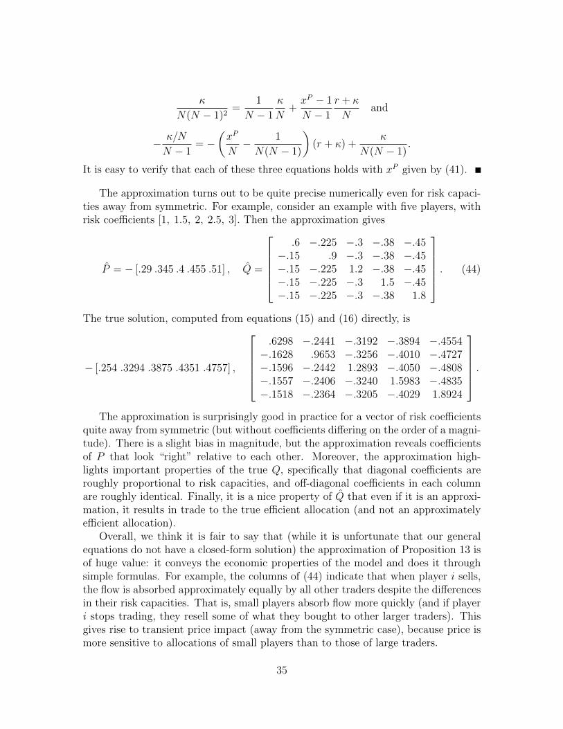
κ
N(N − 1)2=
1
N − 1
κ
N+xP − 1
N − 1
r + κ
Nand
− κ/N
N − 1= −
(xP
N− 1
N(N − 1)
)(r + κ) +
κ
N(N − 1).
It is easy to verify that each of these three equations holds with xP given by (41).
The approximation turns out to be quite precise numerically even for risk capaci-ties away from symmetric. For example, consider an example with five players, withrisk coefficients [1, 1.5, 2, 2.5, 3]. Then the approximation gives
P = − [.29 .345 .4 .455 .51] , Q =
.6 −.225 −.3 −.38 −.45
−.15 .9 −.3 −.38 −.45−.15 −.225 1.2 −.38 −.45−.15 −.225 −.3 1.5 −.45−.15 −.225 −.3 −.38 1.8
. (44)
The true solution, computed from equations (15) and (16) directly, is
− [.254 .3294 .3875 .4351 .4757] ,
.6298 −.2441 −.3192 −.3894 −.4554−.1628 .9653 −.3256 −.4010 −.4727−.1596 −.2442 1.2893 −.4050 −.4808−.1557 −.2406 −.3240 1.5983 −.4835−.1518 −.2364 −.3205 −.4029 1.8924
.The approximation is surprisingly good in practice for a vector of risk coefficients
quite away from symmetric (but without coefficients differing on the order of a magni-tude). There is a slight bias in magnitude, but the approximation reveals coefficientsof P that look “right” relative to each other. Moreover, the approximation high-lights important properties of the true Q, specifically that diagonal coefficients areroughly proportional to risk capacities, and off-diagonal coefficients in each columnare roughly identical. Finally, it is a nice property of Q that even if it is an approxi-mation, it results in trade to the true efficient allocation (and not an approximatelyefficient allocation).
Overall, we think it is fair to say that (while it is unfortunate that our generalequations do not have a closed-form solution) the approximation of Proposition 13 isof huge value: it conveys the economic properties of the model and does it throughsimple formulas. For example, the columns of (44) indicate that when player i sells,the flow is absorbed approximately equally by all other traders despite the differencesin their risk capacities. That is, small players absorb flow more quickly (and if playeri stops trading, they resell some of what they bought to other larger traders). Thisgives rise to transient price impact (away from the symmetric case), because price ismore sensitive to allocations of small players than to those of large traders.
35

Let us reiterate some of the most important on and off-equilibrium propertiesof our model in light of the approximation. First, let us discuss equilibrium pricemomentum.
From (41) we see that the price is less sensitive to the inventories of large playersthan those of small players (recall the players with the most negative εi are thelargest). As we explained above, the intuition is that large players have marketpower and they control their trading rates better, while the small players competewith each other and pay much less attention to the impact of their trades on theprice. Hence, equilibrium price is skewed in favor of large players, relative to first-best, and it tends to first best over time as the allocation converges. Second, letus discuss the speed of trade. The diagonal elements of Q are proportional to riskcoefficients. Hence, in this approximation the speed of trade of individual players isinversely proportional to their risk capacities. The following proposition characterizeseigenvectors and eigenvalues of the approximating matrix Q.
Proposition 14 Suppose that the coefficients of vector ε are strictly increasing and1+ε1 > 0 (that is, players are ordered from largest to smallest, and the risk coefficientof the largest player is b1 = b(1 + ε1) > 0). Then the eigenvalues of matrix Q =κ(I − S/N)(I +Dε) satisfy
κ1 = 0, κ2 ∈ (κ(1 + ε1), κ(1 + ε2)), . . . κN ∈ (κ(1 + εN−1), κ(1 + εN))
and corresponding eigenvectors take the form (for κ′ = κi)
v = [v1, v2, . . . vN ]T with vi =1
1 + εi − κ′/κ. (45)
The decomposition confirms the curious sign pattern we observed in our example(25). Notice that the first i − 1 coefficients of vector vi are positive, in increasingorder, while the remaining coefficients are negative (also in increasing order). Hence,in each eigenvector, large players are on one side of the market while small playersare on the other side. The fewer players there are in the group of small traders, thelarger the corresponding eigenvalue, which corresponds to the speed of trade. Noticethat the first eigenvector is the efficient allocation.
Proof. Consider a vector v = [v1, v2, . . . vN ]T , and let us normalize∑
i(1 + εi)vi = N.
Then Qv = κ[(1 + ε1)v1− 1, . . . (1 + εN)vN − 1]. If v is an eigenvector with eigenvalueκ′, then the coefficients vi satisfy κ((1 + εi)vi − 1) = κ′vi or (45).
For the normalization to hold, we must have∑i
1 + εi
1 + εi − κ′/κ= N. (46)
36

Equation (46) has solution κ′ = 0. In addition, for each i = 2, . . . N, as κ′/κ goesthrough the interval (1 + εi−1, 1 + εi), the sum
1 + εi−1
1 + εi−1 − κ′/κ+
1 + εi
1 + εi − κ′/κ
goes from −∞ to ∞, while the remaining terms of (46) stay finite. Hence, equation(46) has a root κ′ ∈ κ(1 + εi−1, 1 + εi). Corresponding to each of these roots, thereis an eigenvector with coefficients of the form (45). Since we have found N distincteigenvalues κi, and Q is N ×N, we have found all eigenvalues.
Finally, let us turn to off-equilibrium properties, i.e. price impact. From (42),instantaneous price impact (the sensitivity of price to trading flow) of player i isgiven by
I i =b/r
(N − 1)κ
(1− (N − 2)2
N(N − 1)εi)
+O(|ε|2).
Large players (with small εi) have greater price impact than small players. Thisproperty stems from differences in equilibrium strategies - large players trade slowerand hence their flow signals that they have a larger amount waiting to be traded.
Permanent impact reflects simply with the risk capacity of other traders. Finally,as we discussed earlier, the existence of transient impact has to do with the off-diagonal entries of the matrix Q - smaller players, whose allocations have a greaterimpact on price, initially absorb a greater portion of flow than their risk capacitydictates.
5.6 Application: Technical Front-Running.
In Section 4, we saw a basic example of front-running of large trader’s sales. Fringemembers, who start with first-best inventories, pick up supply from other fringe mem-bers (in an instant) and then sell to the large trader. In this particular pattern indi-vidual fringe members have no price impact and hence do not optimize the timing oftheir buying. We now illustrate the process of technical front-running in more detailusing a model of multiple symmetric large players and a fringe. We also illustratehow properties of prices as well as the speed of trade towards the efficient allocationcan be understood through the eigenvector decomposition of the matrix Q.
Consider a market with N−1 large players with identical risk capacities 1/bL anda competitive fringe with risk capacity 1/bF . In this case trading is characterized bythe matrix Q = UKU−1, where
U =
1/bL 1 . . . 1 11/bL −1 . . . 0 1
......
. . ....
...1/bL 0 . . . −1 11/bF 0 . . . 0 1−N
and K = diag [0, κ, . . . , κ, κ], (47)
37

with κ < κ. The price is given by P = ΠU−1, where
Π =
[−1
r, 0, . . . , 0, πB
], where πB =
(N − 1)bF
r + κ.
The eigenvector decomposition of trading dynamics can be understood as follows.The entries of Π correspond to the prices that result from allocations in the cor-responding columns of U. The first column is the efficient allocation. Columns 2through N are misallocations, with coefficients that add up to 0. These eigenvector-misallocations get traded to efficiency at rates given by the eigenvalues κ and κ. Anyallocation X can be represented as a linear combination of eigenvectors, to see howit is traded as well as the resulting price.
From symmetry, any misallocation among the large traders has no effect on theprice. This is illustrated by the zero coefficients 2 through N − 1 of Π; the corre-sponding columns of U span the space of various misallocations among large players.In contrast, any imbalance between the large traders and the fringe leads to a pricethat is different from first best. When the large traders are net sellers, the price isabove first best, as illustrated by the positive value of πB. That is, the price is πB forthe allocation X that corresponds to the last column of U.
Let us illustrate how front-running can happen in this model. With two largeplayers and a fringe, suppose that player 1 wants to sell one unit, while the fringewants to buy one unit. Player 2 wants neither to buy nor sell, so that X0 = [1 0 −1]T .Because player 1 has market power against the fringe, he sells slowly and charges aprice above first best. This can be seen by the positive last component of Π, whichprices the excess inventory of the large players relative to the fringe. Over time, theprice drifts down and converges to first best.
Knowing this, of course, player 2 does not stay at his bliss point. Rather, hesells short initially to the fringe, and buys back from player 1 later. In other words,player 2 front-runs player 1. The mere presence of player 2 in the market changesthe dynamics between player 1 and the fringe. Player 1 trades much faster knowingthat there is a front runner. The trading speed κ between the two large players andthe fringe is faster than the trading speed κ given by (19), which would have resultedhad player 2 been absent.
In this example, the initial allocation can be decomposed into eigenvectors in thefollowing way 1
0−1
=U2 + U3
2=
1/2−1/2
0
+
1/21/2−1
.That is, the allocation X0 = [1 0 − 1]T consists of an imbalance between the largeplayers, and between large players and the fringe. The former gets traded to efficiencymuch more slowly than the latter, with the corresponding convergence rates κ < κ.Thus, at the beginning player 2 will be primarily selling to the fringe, and buying
38
only a little from player 1. The misallocation between the two large players persistsa lot longer than the misallocation between the large traders and the fringe.
6 Common Values.
Our model has correlated private values. In Section 2 we also provided an extensionof the model to incorporate common values, with payoff flows given by (9). While acomplete analysis of this case is beyond the scope of this paper, we conjecture thatwhen the common value components are not too large, the fully separating linearequilibrium of the conditional double auction still exists. The corresponding directrevelation mechanism asks players to report their private signals ξit, and sets pricesand trade flows according to
pt = P (xt − Fξt︸ ︷︷ ︸Xt
), qt = Q(xt − Fξt),
where holdings xt are computed directly from the past history of trades. If player ireports signal ξit + y rather than ξit, the report affects the entire vector Xt that feedsinto the mechanism, and not only component X i
t . As a result, the first-order conditionfor player i to report truthfully becomes
(PF i)Qi + P (QiF i) = 2(AiQF i)T ,
rather than (15), where F i is the ith column of F. Matrix Ai satisfies the same HJBequation (16), while the coefficient ki of the value function is now
ki =tr [ΣFF TΣTAi]
r.
We use these equations to illustrate how common values affect trade via two examples.First, we extend the symmetric result of Proposition 12 to the case of common values.Second, we explore what happens when one particular player has private informationabout fundamentals.
In the symmetric case with bi = b for all i and matrix F as in (10), we can replicateour calculations from the proof of Proposition 12 to obtain
P = − b
Nr1 and Q = κ(I − S/N), where κ =
(N − 2)(1− φ)− φN2(1− φ) + 2φN
.
If φ = 0, κ = (N − 2)/2, as in (37). As φ goes up, κ goes down. Intuitively, as thecommon value concerns increase, trade slows down.28 As before, κ increases in N , so
28Du and Zhu (2013) present an analogous result.
39

more competition speeds up trade. However, in order for the equilibrium with tradeto exist, we need κ > 0, or
φ <N − 2
2(N − 1).
The common value component of signals cannot be too large. As N →∞ this criticalvalue of φ converges to 1/2.
For the asymmetric case, we extend the numerical example in Section 5.1 toprovide some casual intuition. To that end, suppose that
F =
1 0.2 0 0 00 1 0 0 00 0.2 1 0 00 0.2 0 1 00 0.2 0 0 1
rather than the identity matrix, and the rest of the parameters remain unchanged.According to matrix F, traders 1, 3, 4 and 5 have signals about only their privatevalue, while trader 2’s signal contains information about common value that impactsother traders symmetrically. In this case the (P,Q) change to
P = − [0.276, 0.180, 0.439, 0.500, 0.553] ,
Q =
0.503 −0.089 −0.303 −0.370 −0.433−0.062 0.335 −0.113 −0.134 −0.154−0.151 −0.085 1.018 −0.380 −0.450−0.147 −0.082 −0.303 1.259 −0.451−0.143 −0.079 −0.299 −0.375 1.487
.
Comparison to the example in Section 5.1 reveals the following three effects ofcommon-value information in the signals of trader 2. First, trade gets slower overall.This can be seen by noticing that all entries in Q get closer to 0.29 Second, commonvalue can create a reversal in the speed of trade: trader 2 now trades slower thantrader 1 even though he has higher inventory costs. This is because the common-valueinformation significantly increases player 2’s price impact.30 Finally, the off-diagonalelements of Q change in the following way: when trader 2 sells, his flow is stillabsorbed approximately equally by all other traders. But when others trade, trader 2
29A general pattern we observe when we introduce positive off-diagonal elements in F is that thediagonal entries of Q get smaller; the exact pattern for off-diagonal terms is more complicated.
30If player i changes the announcement of his shock by y, the mechanisms’ perception of the vectorX changes by F iy, and hence player i’s flow changes by QiF iy. At the same time, price changes by
PF iy. Hence player i’s instantaneous price impact with common-value information is −PF i/(QiF i).For player 2 in our example, instantaneous price impact is 2.2 and significantly higher than thosefor other players.
40

absorbs a disproportionately small portion of their flow. Again, trades of 2 are sloweddown by the high price impact. Intuitively, other players may be worried that thewillingness to trade by player 2 is a signal of unfavorable common-value information.
7 Discussion
There is a large literature in financial mathematics that focuses on optimal tradingunder various transaction costs and microstructure frictions. The focus of this lit-erature is largely on optimal behavior of an individual trader given a realistic priceprocess, and a realistic model of how trades affect prices - as in Almgren and Chriss(2001). Prices are often modeled as an arithmetic Brownian motion (so they may benegative) - as Almgren and Li (2016) argue, while geometric Brownian motion is amore realistic representation of prices, arithmetic Brownian motion is an adequateand tractable representation of prices for the time horizons over which trades takeplace (e.g. over a day). Trades have instantaneous and permanent price impact, andpossibly transient price impact characterized by an appropriate decay kernel, as inGatheral, Schied and Slynko (2011). While in practice price impact may not be linearin flow - e.g. Almgren, Thum, Hauptmann, and Li (2005) document that it may beconcave for small trades - linearity is a common assumption. Concavity may reflecttransaction costs due to discreteness of micro-level microstructure, but linearity leadsto greater tractability, and certain results suggest that only linearity is consistent withabsence of arbitrage (e.g. see Gatheral (2010) and Huberman and Stanzl (2004)).
Our paper follows this literature’s focus on realistic price behavior. However, in-stead of assuming that prices are Brownian and that trades have instantaneous andpermanent impact, we derive these properties in equilibrium. That is, we model amarket in which individual participants have objectives similar to those of individualtraders in Bank, Soner and Voß (2016) - they have evolving hedging motives for trad-ing individual assets - but we derive price behavior in these markets, and characterizeprice impact faced by individual participants. We obtain price behavior consistentwith the assumptions of this literature, and because we model the interaction of alltraders, we tie the properties of price impact to market characteristics (i.e. the num-ber of market participants and their market power). Thus, our model can be thoughtof as an explanation for why price impact has a particular form, and how it is tied tomarket characteristics.
In order to characterize equilibrium in a tractable manner, we assume that tradingis not anonymous, but rather players can condition their behavior on who they aretrading against. This assumption is not completely realistic, even though it givesplayers information that traders would like to know, since flow of large investors tendsto be much more persistent than that of small traders. However, with this assumptionwe get important benefits. First, we obtain a stationary characterization of equilibria- market liquidity does not change stochastically depending on the active players inthe market. Second, we get a characterization of price impact that depends only on
41

the allocation of market power among players, and not on trading needs or activity.Finally, in solving the model, we avoid the complex issue of filtering that playerswould otherwise need to perform to infer the source of trades from price behavior.Moreover, our paper makes a methodological contribution – we model trading as aconditional double auction to allow players to take into account who they are tradingagainst.
By modeling the entire market, we are able to answer questions not just aboutoptimal execution of transactions, but also about welfare, determinants of liquidity,and strategic interactions among traders. Of course, we are not the first ones tomodel the whole market - Vayanos (1999), Du and Zhu (2013) and Kyle, Obizhaevaand Wang (2014) model symmetric markets, while Malamud and Rostek (2014) andLambert, Ostrovsky and Panov (2016) model asymmetric markets in a one-shot set-ting - we model dynamics of an asymmetric market. Large traders trade slower, andso their flow is highly persistent, consistently with empirical literature. This leadsto price momentum, which is absent from symmetric models. Momentum from theflow of large traders gives rise to the front-running phenomenon in our model. Forexample, some players may sell short together with a large trader early on, and buyback later after the price drifts down. The front-running phenomenon helps reconcilethe persistence of institutional flow and price momentum with market efficiency - aquestion addressed also in Farmer et al (2006). Our answer is that while flow of largetraders is persistent, market price reacts right away fully to the news of the entiresupply of a large trader, as the front runners trade with the large trader. That is, themarket recognizes the entire quantity that the large player would like to sell. How-ever, momentum still exists, reflecting limits to arbitrage. Front runners recognizemomentum, but they are already exploiting it to the fullest given their risk capacity.Overall, our model suggests that the front-running phenomenon not only improvesefficiency, as prices deviate from efficiency less and converge to efficiency faster inmore competitive markets, but that it can be good for large traders to be front run.That is, while front runners take away large players’ profits, they also make it easierto execute transactions with less price impact.
There are a number of questions that are at the center of the debate about financialmarket regulation, but which cannot be addressed definitively given existing theory.While our model is too simple for many of these questions, with the focus on theentire market and with explicit modeling of players’ utilities, it can be used to thinkabout a subset of them. One question is about opaque versus transparent markets.Our model is transparent, because traders observe flows of other traders, but howwould the equilibrium change if players did not see that? Presumably, large traderswould have lower price impact, and so they could trade faster, as they could hidetheir flow behind that of small traders. If so, then what is the effect of separation offlows of large and small traders, e.g. when some market makers pay retail brokeragesto execute retail flow. Does this improve execution prices of retail traders, as thesemarket makers claim? It seems quite likely, since our model suggests that trades of
42

small players should have lower price impact. However, another implication is that theresidual flow has a greater fraction of trades of institutional investors, and is thereforemore persistent. This leads to lower market liquidity overall, and this equilibriumeffect could harm retail investors who seem to be getting better execution.
Our model approximates flow as continuous, whereas in practice transactions arediscrete. Is there any relationship, then, between our results and bid-ask spreads? Po-tentially there is a useful link. Suppose bid-ask spreads are set by liquidity providerswho take into account tradeoff between risk and profit that they can make from facili-tating transactions. Then the size of the bid-ask spread should depend on competitionamong liquidity providers, as well as properties of the flow, e.g. persistence, and ourmodel speaks to those properties.
8 Conclusions
We would like to summarize the main contribution of the paper. First, the papermakes a methodological contribution. We introduce a linear-quadratic model of con-ditional double auctions in a market where traders have hedging motives to trade.This model provides a tractable way to analyze the market with heterogeneous par-ticipants. Second, we characterize important on and off-equilibrium properties oftrade. On equilibrium players trade slowly to reduce price impact, and flow of largertraders is more persistent than that of small traders. This heterogeneous behaviorleads to price momentum, and creates incentives for players to know the source offlow for technical front-running. Off equilibrium, our characterization of price impactmatches the classical assumptions of financial mathematics literature - trades have in-stantaneous, permanent and transient impact. Our results have welfare implications- for example, we show that market power, characterized as the ability to coordinatethe execution of a large number of trades, may be detrimental to players’ welfare ina fully transparent market, i.e. when large traders cannot hide flow behind those ofsmall traders.
43

ONLINE APPENDIX, NOT FOR PUBLICATION.
A Appendix A: A Microfoundation of Quadratic
Preferences.
In this section we microfound our model with quadratic preferences by laying out amore natural model with exponential utilities, in which players trade to hedge privateshocks that expose them to a common risk factor. We show that the equilibriumequations of the linear-quadratic model match those of the exponential model in thespecial case when the shocks that expose players to the common risk factor becomesmall. In this sense, the exponential model is more general, but the linear-quadraticmodel provides a clean special case as the equilibrium dynamics, characterized by thepair (P,Q), depend only on the players’ risk capacities and not the sizes of shocksthat individual players receive, or the correlation among shocks.
We then extend the model to also allow shocks to carry information about acommon component of value. We confirm the result of Du and Zhu (2013) that insymmetric markets, as the players get more information about common fundamentals,the speed of trade slows down. In general asymmetric markets, equilibrium in thismore general setting is characterized by a system of equations analogous to what wedescribed in the text, with only one extra term.
A.1 The Exponential Model.
Consider a model in which all players i = 1, . . . N have exponential utility
− exp(−αict),
where αi > 0 is the coefficient of absolute risk aversion. Players consume continuouslyand have a common discount rate r, which is also the risk-free rate in the market.
Players have private information about their risk exposure X it to a common Brow-
nian risk factor dWt. Risk exposure changes due to shocks driven by Brownian motionsZ = [Z1
t , . . . ZNt ], independent among each other and of Wt with a vector of volatilities
σ. Risk exposures can be traded in the market. We consider a (linear, stationary)equilibrium, in which players announce their risk exposures, and given a vector ofannouncements Xt, the trading flows are given by QXt, and the market price is givenby PXt. Then the risk exposures follow
dXt = Σ dZt −QXt dt
where Σ is the diagonal matrix with the elements of σ on the diagonal. The wealthof agent i follows
dwit = (rwit − cit) dt+ (PXt)(QiXt) dt+X i
t dWt,
44

where cit is the consumption of player i.Conjecture that the equilibrium value function of player i takes the form
− 1
rexp(−rαi (wit +XT
t AiXt + ki)︸ ︷︷ ︸
vit
). (48)
Thendvit = (rwit − cit) dt+ (PXt)(Q
iXt) dt+X it dWt
+2XTt A
i(Σ dZt −QXt dt) + tr [ΣΣTAi] dt.
In order to write down the HJB equation for player i, we must consider X it of the
form Xt + 1iy, where 1i is the i-th coordinate vector and y is the amount by whichplayer i lies.
Then the HJB equation of player i is
− exp(−rαivi) = maxc, X=X+1iy
− exp(−αic)
+αi exp(−rαivi)(rwi − ci + (PX)(QiX)− 2XTAiQX + tr [ΣΣTAi]
)−r(α
i)2
2exp(−rαivi)
(4XTAiΣΣTAiX + (X i)2
).
The term 4XTAiΣΣTAiX is the incremental variance of vit from the volatility ofthe entire vector Xt.
31
The first-order condition with respect to c is
exp(−αic) = exp(−rαivi) ⇔ −c = −r(wi +XTAiX + ki).
Given this, the HJB equation simplifies to
0 = maxX=X+1iy
−r(XTAiX + ki) + (PX)(QiX)− 2XTAiQX + tr [ΣΣTAi]
− rαi
2
(4XTAiΣΣTAiX + (X i)2
). (49)
Separating the first-order condition, we obtain matrix equations that characterizestationary linear equilibria in this model. We summarize them in the following propo-sition.
31This expression assumes that Ai is symmetric, otherwise the second instance of Ai would needto be replaced with (Ai)T .
45

Proposition 15 Stationary linear equilibria of the exponential model are character-ized by the equations
P iQi +QiiP = 2(AiQi)T , rki = tr [ΣΣTAi], (50)
and rAi + AiQ+QAi =P TQi + (Qi)TP
2− rαi
21ii − 2rαiAiΣΣTAi. (51)
Proof. Equation (49) must hold for all vectors X ∈ RN . To ensure that, the coeffi-cients on the constant term as well as the terms of the form XjXk must match, andthe first-order condition with respect to y must hold at y = 0. From those conditions,we obtain (50) and (51).
The system of (50) and (51) is different from equations (15) and (16) in the linear-quadratic model only in the term 2rαiAiΣΣTAi. Parameter bi in the linear-quadraticmodel corresponds to rαi in the exponential model, i.e. it reflects the players’ ca-pacities to wait and absorb risk waiting for a better price to hedge at. In the limitas σ → 0, the equations in the exponential model become identical to those in thelinear-quadratic model. Thus, the linear-quadratic model is a special case of theexponential model. We summarize this finding in the following proposition.
Proposition 16 Any solution of the linear-quadratic model solves equations (50) and(51) in the limit as |Σ| → 0.
Proof. The conclusion follows immediately, since the term that distinguishes the twosets of equations converges to 0 as |Σ| → 0.
Even though the exponential case is more general, the linear-quadratic modelprovides a much cleaner picture of equilibrium dynamics, as the equilibrium equationsdepend only on the players’ risk capacities and not the distribution of shocks. Thismakes our benchmark case particularly attractive. Nevertheless, in order to providea more complete picture, we present a couple of computed examples for the generalcase at the end of this section.
A.2 Examples.
We return to the example from Section 5 to explore how the extra term in (51) affectsprices and the rates of trading. Recall that the risk coefficients are [b1, b2, b3, b4, b5] =[1, 1.5, 2, 2.5, 3] and r = 1 in that example. Then the coefficients of absolute riskaversion are also [α1, α2, α3, α4, α5] = [1, 1.5, 2, 2.5, 3]. Assume that Σ = 0.1I, i.e.shocks to individual players are uncorrelated and have volatility 0.1.
Then, we have
P = [−.257, −.334, −.394, −.443, −.485].
46

The price sensitivities to the allocations of all players increase slightly. Trading dy-namics are now characterized by
Q =
0.619 −0.243 −0.318 −0.388 −0.454−0.161 0.953 −0.324 −0.400 −0.472−0.157 −0.242 1.278 −0.403 −0.479−0.153 −0.237 −0.320 1.589 −0.481−0.147 −0.231 −0.315 −0.398 1.886
.The speed of trading slows down somewhat, but qualitatively and quantitatively thesolution looks similar to our baseline model.
Now, consider Σ = diag [0.1, 0.3, 0.3, 0.1, 0.1]. We raise the fundamental needs totrade of players 2 and 3, while keeping shocks to everyone else the same. Now, players1, 4 and 5 can provide liquidity to players 2 and 3, and help them share risks. Thenthe trading dynamics are characterized by the price vector
P = [−.265, −.358, −.426, −.463, −.507]
and the trading matrix
Q =
0.572 −0.246 −0.326 −0.374 −0.437−0.146 0.951 −0.322 −0.374 −0.445−0.131 −0.222 1.312 −0.364 −0.439−0.150 −0.244 −0.334 1.500 −0.467−0.145 −0.239 −0.330 −0.387 1.787
.The price impact of shocks rises and trade tends to slow down, especially for playerswho are hit by relatively smaller shocks.
These examples seem to imply that the more general model with exponentialutility does not add much intuition about market dynamics on top of what the baselinelinear-quadratic model already tells us. Of course, there may be interesting effectsthat we are overlooking.
B Appendix B: Omitted proofs
B.1 Mechanisms for Trading.
Proof of Proposition 1. Equations (11) can be represented as
π = p1 + Πq, (52)
where π is a vector of intercepts, 1 is a vector of ones, and Π is a matrix withcoefficients πij and zeros on the diagonal. Equation (52) has a solution for all vectorsπ if and only if the image of the set of all flow vectors (i.e. vectors whose entries
47

add up to 0) q under Π has dimension N − 1 and does not contain vector 1. In thiscase, a unique pair (p, q) corresponds to each vector π, and statements 1 and 2 followimmediately.
Let us show that if either the image of flow vectors under Π has dimension lessthan N − 1, of if the image contains 1, then statements 1 and 2 are both false. If thedimension is less than N − 1, then the pre-image of 0 has dimension of at least 1.Then 1 is false as (0, q) is a solution for any q in the pre-image, and 2 is also false, asthe span of the image together with vector 1 has dimension at most N − 1.
If vector 1 is in the image of flow vectors under Π, e.g. 1 = Πq, then any pair(p,−pq) is a solution to 0 = p1 + Πq, so statement 1 is false. Likewise, statement 2 isfalse since the span of the image (which does not change if we include vector 1) hasdimension at most N − 1.
Proof of Proposition 2. First, let us demonstrate equivalence of the first twostatements. If the mechanism (P,Q) is not acceptable, i.e. there exists a nonzerovector X in the null space of Q such that PX = 0, then QPX = 0, so QP is notinvertible. Conversely, if QP is not invertible, i.e. QPX = 0 for X 6= 0, then QX = 0also since if all flows except for that of player 1 are zero, then the flow of player 1must also be 0. Thus, X is in the null space of Q and PX = 0, so (P,Q) is notacceptable. This shows that the first two statements are equivalent.
Second, let us demonstrate the equivalence of the last two statements. If QP
is invertible, then X = (QP )−1(p, q2, . . . qN), where p = PX and q = QX, so theallocation X can be inferred from the pair (p, q). If QP is not invertible, then the setof (p, q2, . . . qN) that corresponds to all X has dimension of at most N −1. Since q1 isa linear combination of q2, . . . qN , the set of (p, q) has the same dimension. Hence, wecannot infer X from (p, q). This shows that the last two statements are equivalent.
Proof of Theorem 1. Let us first identify the one-to-one map between acceptableprofiles and mechanisms. Consider any acceptable stationary linear revealing profileof strategies of the conditional double auction. Then equation (52) has a uniquesolution. From market clearing, (52) can be written as
1 π12 . . . π1N
1 −π21 . . . π2N − π21
1...
...1 πN2 − πN1 . . . −πN1
︸ ︷︷ ︸
Π
pq2
...qN
=
π1
π2
...πN
, (53)
where matrix Π is obtained by placing 1 in the first column and by subtracting thefirst column of Π from each remaining column. The profile is acceptable if and only ifΠ is invertible and all πi are nonzero. Hence, QP = Π−1 diag(πi), i.e. the pair (P,Q)is uniquely defined from the acceptable profile {πi, πij, i 6= j}. The pair (P,Q)
48

must also be acceptable. Indeed, if X is in the null space of Q and PX = 0, thenΠ−1 diag(1/πi)X = 0 implies that X = 0.
Let us show that the mechanism we just constructed has no stationary allocationsX 6= 0 that have X i = 0 for one of the players. Notice that (QP )−1 = diag(1/πi)Πhas no zeros in column 1. If so, then for any stationary allocation, X 6= 0, thecorresponding price is p 6= 0, so X = (QP )−1(p, 0 . . . 0)T , and all elements of X arenonzero since column 1 of (QP )−1 has no zeros. The converse is also true: if X 6= 0is a stationary allocation of an acceptable mechanism (P,Q), and if X i 6= 0 for all i,then the first column of (QP )−1 equals (1/p)X, and so it has no zeros.
Conversely, the pair (P,Q) is acceptable if and only if QP is invertible by Propo-sition 2. Since the corresponding profile must satisfy diag(πi)(QP )−1 = Π, and sincethe first column of Π must contain ones, we can obtain the corresponding profileas follows. We must set πi to the inverse of the i-th entry in column 1 of (QP )−1,and then divide each row i of (QP )−1 by πi to obtain Π. Then the first column of Πcontains ones, and we can infer the slopes πi1 from the diagonal of Π, and infer theremaining ones from the remaining entries. In order for this procedure to work, it isnecessary (and sufficient) for the first column of (QP )−1 to have no zeros. We knowthat this is the case, because for any stationary allocation X 6= 0 of Q, all elementsX i are nonzero.
Now, let us prove strategic equivalence of the corresponding mechanism and pro-file. In a mechanism, given the allocation X−i of other players, player i has thechoice between flow and price pairs given by (PX,QX | X = X + 1iy). In the cor-responding profile (πi, πij, j 6= i), player i also has the same one-dimensional set ofprice-flow pairs, which he can attain by changing the intercept from πi = πiX i toπi = πi(X i + y). Let us prove that player i does not have any more choices than that(i.e. he cannot achieve any price-flow pair outside this set by also changing the slopesπij of his supply-demand function).
Any price-flow pair (p, q) that can be attained by a deviation of player i mustsatisfy the N −1 equations from (53), with equation i excluded. Since these are inde-pendent equations (when the matrix Π is invertible), they define a set of pairs (p, q) ofdimensions 1. Hence, any price-flow pair that player i can generate, can be attainedby changing only the intercept πi. We conclude that corresponding mechanism andprofile must be strategically equivalent.32
B.2 Equilibrium Characterization.
Proof of Proposition 3. We have to prove that the truth-telling strategy maxi-mizes the utility of any player i. For an arbitrary strategy {yt, t ≥ 0}, which specifies
32Of course, player i may be able to choose a supply-demand function that does not lead to anyallocation at all.
49
the misrepresentation yt of player i’s allocation for any history {Xs, s ∈ [0, t]} ofallocations, consider the process
Gt =
∫ t
0
e−rs(
(PXs + piys)(QiXs + qiiys)−
bi
2(X i
s)2
)ds+ e−rtf i(Xt).
Then the conditions pi < 0 and qii > 0 ensure that yt = 0 maximizes the drift of Gt,and (13) ensures that the maximal drift of Gt equals 0. That is, the process Gt isalways a supermartingale, and a martingale under the truth-telling strategy.
Now, since the process X defined by (12) is nonexplosive, it follows that when allplayers follow the truthtelling strategies
E[e−rtf i(Xt)]→ 0
as t→∞ . Therefore, player i’s expected payoff under the truthtelling strategy is
E
[∫ ∞0
e−rs(
(PXs)(QiXs)−
bi
2(X i
s)2
)ds
]= E[G∞] = G0 = f i(X0).
Consider any alternative strategy {yt, t ≥ 0} that satisfies the no-Ponzi con-dition E[e−rtX2
t ] → 0 as t → ∞. Then for any quadratic value function f i(X),E[e−rtf i(Xt)]→ 0 as t→∞. It follows then that player i’s payoff under this strategyis
E
[∫ ∞0
e−rs(
(PXs + piys)(QiXs + qiiys)−
bi
2(X i
s)2
)ds
]= E[G∞] ≤ G0 = f i(X0).
Thus, truth-telling is optimal. This completes the proof of Proposition 3.
Proof of Proposition 4. Individual fringe members do not have price impact, andan individual may choose to hold allocation x different from that of the rest of thefringe, XN . If x = XN , then individual continuation utility is fN(X) = XTANX+kN
and in general the value function takes the form XTANX + (x−XN)PX + kN , sincetrading x−XN generates the income of (x−XN)PX.
Since there is no price impact, we treat dynamic choice of an individual fringemember simply as choosing x at all times. Then the HJB equation is written as
maxx
−bF
2x2 − r(XTANX + (x−XN)PX + kN) + (PX)(QNX)
−2XTANQX − (x−XN)PQX + tr [ΣΣTAN ] = 0.
The first-order condition
−bFx− P (rX +QX) = 0
must hold at x = XN , so it follows that (17) must hold. Notice also that (kN , AN)must satisfy the same equations as before, (16).
50

B.3 Large Player and Fringe.
Proof of Proposition 5. With one large trader and the fringe, the mechanism isdescribed by the four parameters:
Q =
[qL −qF−qL qF
], P = [pL, pF ]
First, fringe’s optimality condition (17) is
rpL + pLqL − pF qL = 0 and rpF − pLqF + pF qF + bF = 0. (54)
Second, for the large player, equation (16) implies that
ra11 − 2a12qL + 2a11qL = −1
2bL + pLqL (55)
ra12 − a11qF + a12 (qL + qF )− a22qL =pF qL − pLqF
2(56)
ra22 − 2a12qF + 2a22qF = −pF qF (57)
and the first-order conditions (15) are
pLqL = qLa11 − qLa12 and pF qL − pLqF = 2a12qL − 2a22qL. (58)
Using (58), we can transform (55), (56) and (57) to
ra11 = −bL/2− pLqLra12 = pLqF
ra22qL = −pLq2F
and plugging coefficients of large player’s value function into (58), we get
rpLqL = −(bL/2 + pLqL + pLqF )qL and rpF qL − rpLqF = 2(qL + qF )pLqF .
Notice that (54) cannot hold with pL = pF , so
qL =rpL
pF − pLand qF =
rpF + bF
pL − pF.
Plugging these into the first-order conditions for the large player, we obtain (if qL 6=0)33
bL
2bF=
pLpF − pL
and 1/2 =pF + bF/r
pL − pF.
33If qL = 0, then the corresponding solution is the degenerate equilibrium,
pL = 0, pF = −bF
r, qL = qF = 0 and AL =
1
r
[−bL 0
0 0
].
51
This leads to a system of linear equations in pF and pL, which have a unique solution
pL = − bLbF
r(3bF + bL)and pF = −(2bF + bL)bF
r(3bF + bL).
Then
qF =r
2, qL =
r
2
bL
bF, and AL =
bF
2r (3bF + bL)
[−3bL −bL−bL bF
].
The welfare of the fringe can found from equation (16). We have
raF22 − 2aF12qF + 2aF22qF = −1
2bF + pF qF
raF12 − aF22qF + a12 (qL + qF )− a11qL =pLqF − pF qL
2raF11 − 2aF12qL + 2aF11qL = −pLqL,
hence
AF =1
2
bF
r (3bF + bL) (2bF + bL)
[(bL)2 −bLbF−bLbF −
((bL)2 + 5bLbF + 5(bF )2
) ] .
B.4 Welfare Results.
In order to prove Proposition 7, we need to be able to evaluate the welfare of a portionof the fringe when the fringe is heterogeneous. Consider a market with N − 1 largeplayers and the fringe, in which the joint welfare of the fringe is characterized by theN -by-N matrix AN . Consider two parts of the fringe with risk capacities β1/b
N andβ2/b
N , respectively, with β1 + β2 = 1. Let us determine the value function matricesA1 and A2 for the two parts of the fringe (these are (N + 1) × (N + 1) matrices).How would an initial allocation X = (X1, . . . XN−1, X1, X2) get traded? We knowthat part 1 of the fringe instantaneously sells
X1 − β1(X1 + X2) (59)
at price PX, where X = (X1, . . . XN−1, X1 + X2). After the initial trade, conditionalon the absence of future shocks, the two parts of the fringe get utilities β1X
TANXand β2X
TANX, respectively. Thus, prior to the trade, the welfare of the first part ofthe fringe is given by
XT A1X = β1XTANX + (PX)((1− β1)X1 − β1X
2). (60)
52

Proof of Proposition 7. Let us normalize market risk capacity to 1 = β1 + β2,where β1 = 1/bL and β2 = 1/bF are risk capacities of the large player and the fringe,respectively. Then welfare of the large player is given by
AL =1
2r(2β1 + 1)
[−3 −1−1 β1/β2
]. (61)
Let us compare this with the welfare of this group of players under perfect competi-tion. The welfare of a fringe of risk capacity 1 is expressed by the matrix A1 = −1/(2r)and the price is given by P = −1/r, thus the welfare of the first part of the fringe(with risk capacity β1 = βL) by (60) is
−β1(X1 + X2)2
2r− X1 + X2
r((1− β1)X1 − β1X
2),
i.e. it is expressed by the matrix
A1 =1
2r
[β1 − 2 β1 − 1β1 − 1 β1
]Compare with (61). Given shocks of standard deviation (σ1, σ2) with correlation ρ,2r(2β1 + 1) times the difference in welfare between the fringe and the large player inthese two games is
(2β1 + 1)((β1 − 2)σ2
1 + 2(β1 − 1)σ1σ2ρ+ β1σ22
)+ 3σ2
1 + 2σ1σ2ρ−β1
1− β1
σ22 =
(β1 − 1)(2β1 − 1)σ21 + 2(2β1 − 1)β1σ1σ2ρ−
β21(2β1 − 1)
1− β1
σ22 =
2β1 − 1
1− β1
(−(1− β1)2σ2
1 + 2β1(1− β1)σ1σ2ρ− β21σ
22
)︸ ︷︷ ︸≤0
The quantity in parentheses is minus the variance of
(1− β1)σ1 dZ1t − β1σ2 dZ
2t ,
which is always non-positive (zero only if ρ = 1 and σ1/β1 = σ2/(1− β1), i.e. shocksare such that no trade is required to achieve first best).
Therefore, if β1 < 1/2 then the welfare of the fringe before merger is greater thanthe utility of this segment after merger.
Proof of Proposition 8. Denote q = κ/κ(r/2). Then fringe optimality impliesthat
P + bF1F + PQ = 0 ⇒ [pL, pF ] = − [qbL, bF + qbL]
1 + qbL/bF + q. (62)
53
Given this, the large player’s value function can be found by solving (16). We findthat the large player’s value function is characterized by the matrix
AL =1
1 + 2q(1 + bL/bF )
[−bL/2− qbL + qpLb
L/bF −q(bL + pL)−q(bL + pL) qbF/bL(bL + pL)
].
We would like to find the selling rate q that maximizes
[1 − 1]AL[
1−1
]=−bL/2(1 + qbL/bF + q) + q(bL + bF )
(1 + qbL/bF + q)(1 + 2q(1 + bL/bF )),
an expression obtained by plugging in pL from (62). The first-order condition is givenby the quadratic equation
bF + 2qbL − q2(bL − (bL)2/bF + 2bF ) = 0,
For the equilibrium value of q = r/2, the left-hand side is positive, (2bF + bL)(bF +bL)/4 > 0, so the large player would prefer to commit to a faster selling rate. If 2bF >bL (i.e. the large player is more than 1/3 of the market), then bL− (bL)2/bF + 2bF > 0so the left-hand side goes to minus infinity as q →∞. In this case, the optimal sellingrate corresponds to a finite root on [r/2,∞). If 2bF < bL (i.e. the large player is lessthan 1/3 of the market), then the optimal selling rate is infinity.
Proof of Proposition 9. Consider a market in which aggregate shock is σ dZt perunit of risk capacity, and the large player with bL = 1 (without loss of generality)gets shock σL dZt + σ dZt. Then the fringe, with risk coefficient bF , gets the shocks((1 + 1/bF )σ − σL) dZt − σ dZt. Then
AL =bF
2r(3bF + 1)
[−3 −1−1 bF
],
so the large player’s welfare is
bF
2r(3bF + 1)
(−3(σ2
L + σ2)− 2(σL
(bF + 1
bFσ − σL
)+ σ2) + bF (
(bF + 1
bFσ − σL
)2
+ σ2)
)
=(bF )2 − bF
2r(3bF + 1)
(σ2 + (σL − σ)2
)+σ2 − 2σσL
2r.
Differentiating (bF )2−bF3bF+1
with respect to bF , we obtain
(2bF − 1)(3bF + 1)− 3((bF )2 − bF )
(3bF + 1)2=
3(bF )2 + 2bF − 1
(3bF + 1)2=
(3bF − 1)(bF + 1)
(3bF + 1)2,
which is less than 0 if and only if bF < 1/3. Hence, as the size of the fringe increases(i.e. bF falls), the welfare of the large player rises if bF < 1/3, i.e. the large player isless than 1/4 of the market.
54

B.5 General Characterization.
Proof of Lemma 2. First, let us first justify that the coefficients of the matrixAi = UTAi U are given by (23). Multiplying (16) by UT on the left and U on theright, we obtain
rAi + AiK +KAi =(PU)TU iK + (U iK)TPU
2− bi
2(U i)TU i.
In position jk, the left-hand side has (r + κk + κj)aijk and the right-hand side,
((PUk)uijκj + (PU j)uikκk − biuijuik)/2. Hence,
aijk =−biuijuik + (PU j)uikκk + (PUk)uijκj
2(r + κk + κj).
To express the first-order conditions using Ai, notice that
AiQi = (U−1)T Ai U−1U︸ ︷︷ ︸I
K(U−1)i ⇒ (AiQi)TU = ((U−1)i)TKAi.
Multiplying the first-order condition (15) by U on the right-hand side, we obtain
piU iK + (U iK(U−1)i)︸ ︷︷ ︸qii
PU = 2((U−1)i)TKAi.
Entry k of this vector equation is given by
piκkuik︸ ︷︷ ︸
uikκkPUr+κk+K
r+κk+K(U−1)i
+ (U iK(U−1)i)︸ ︷︷ ︸qii, or (U i
K(r+κk+K)
r+κk+K(U−1)i)
PUk =
−uikbiU i K
r + κk +K(U−1)i+uikκkPU
K
r + κk +K(U−1)i+(PUk)U i K2
r + κk +K(U−1)i,
where Kr+κk+K
is the matrix that has entriesκj
r+κk+κj, j = 1 . . . N, on the diagonal.
Performing some cancellations, we obtain
uikκkPUr + κk
r + κk +K(U−1)i + uikbi
(U i K
r + κk +K(U−1)i
)=
−(r + κk)
(U i K
r + κk +K(U−1)i
)(PUk)
or
uik
(bi + κk(r + κk)
PU 1r+κk+K
(U−1)i
U i Kr+κk+K
(U−1)i
)= −(r + κk)PU
k
55

Proof of Proposition 12. From symmetry, equilibrium pair (P,Q) is characterizedby two parameters p and κ, and takes the form
P = p1, Q = κ(I − S/N).
Then, from symmetry player 1’s value function is characterized by the matrix
A1 =
a11 a12 . . . a12
a12 a22 . . . a22...
......
a12 a22 . . . a22
From (16), the coefficients of matrix A1 satisfy the equations
ra11 + 2κN − 1
Na11 − 2κ
N − 1
Na12 = − b
2+ pκ
N − 1
N
ra12 + κa12 − κN − 1
Na22 −
κ
Na11 = pκ
N − 2
2N
ra22 + 2κ
Na22 − 2
κ
Na12 = −p κ
N.
From (15), the first-order conditions are
2κN − 1
Na11 − 2κ
N − 1
Na12 = 2pκ
N − 1
N
2κN − 1
Na12 − 2κ
N − 1
Na22 = pκ
N − 2
N.
Using the first-order conditions to eliminate the differences a11 − a12 and a12 − a22
from the value function equations, we obtain
ra11 = − b2− pκN − 1
N
ra12 =pκ
N
ra22 = − pκ
N(N − 1).
After substitutions, the first-order conditions become
κ
(− b
2− pκ
)= rpκ and pκ2 = rpκ
N − 2
2.
If κ 6= 0, then we obtain34
p = − b
Nrand κ = r
N − 2
2.
34If κ = 0, then the solution is degenerate with a11 = −b/2, a12 = a22 = 0, and p can be anynumber.
56

Notice that for any vector X whose coefficients add up to 0, SX = 0, so QX = κX,and hence any misallocation gets traded to efficiency exponentially at rate κ. Thiscompletes the proof.
57

Bibliography.
Almgren, R. and N. Chriss (2001) “Optimal Execution of Portfolio Transactions,”Journal of Risk. 3(2), 5–39.
Almgren, R. and T. M. Li, (2016) “Option hedging with smooth market impact,”forthcoming in Market Microstructure and Liquidity.
Almgren, R., C. Thum, E. Hauptmann and H. Li (2005) “Equity Market Impact,”Risk July, 57–62.
Back, K. (1992) “Insider Trading in Continuous Time,” Review of Financial Stud-ies, 5, 387–409.
Back, K., C. H. Cao, and G. A. Willard (2000) “Imperfect Competition amongInformed Traders,” Journal of Finance, 55, 2117–2155.
Bank, P., M. Soner, M. Voß (2016) “Hedging with Temporary Price Impact,”Mathematical Finance.
Bouchaud, J.-P. (2010). “Price Impact.” Encyclopedia of Quantitative Finance.DOI: 10.1002/9780470061602.eqf18006
Budish, E., P. Cramton and J. Shim, (2015) “The High-Frequency Trading ArmsRace: Frequent Batch Auctions as a Market Design Response,” Quarterly Journal ofEconomics 130(4), 1547–1621.
Caldentey, R. and E. Stacchetti (2010) “Insider Trading with a Random Deadline,”Econometrica, 78(1), 245–283.
Du, Songzi and Haoxiang Zhu (2013) “Dynamic Ex Post Equilibrium, Welfareand Optimal Trading Frequency in Double Auctions,” working paper, MIT.
Farmer, J. D., A. Gerig, F. Lillo, and S. Mike (2006) “Market Efficiency and theLong-memory of Supply and Demand: is Price Impact Variable and Permanent orFixed and Temporary?” Quantitative Finance 6, 107–112.
Gatheral, J. (2010) “No-Dynamic-Arbitrage and Market Impact.” QuantitativeFinance 10(7), 749–759
Gatheral, J., A. Schied and A. Slynko (2011) “Transient linear price impact andFredholm integral equations,” Mathematical Finance, 22(3), 445–474.
Glosten, L. R. and P. R. Milgrom (1985) “Bid, Ask and Transaction Prices ina Specialist Market with Heterogenously Informed Traders,” Journal of FinancialEconomics, 14, 71–100.
Huberman, Gur, and Werner Stanzl (2004) “Price Manipulation and Quasi-arbitrage,”Econometrica 72, 1247–1275.
Kyle, A. S. (1985) “Continuous Auctions and Insider Trading,” Econometrica, 15,1315–1335.
58

Kyle, A. S. (1989) “Informed Speculation with Imperfect Competition,” Reviewof Economic Studies, 56, 317-355.
Kyle, A. S., A. A. Obizhaeva, and Y. Wang (2014) “Smooth Trading with Over-confidence and Market Power,” working paper.
Lambert, N., M. Ostrovsky and M. Panov (2016) “Strategic Trading in Informa-tionally Complex Environments,” working paper, Stanford GSB.
Leland, Hayne and Pyle, David H, (1977), Informational Asymmetries, FinancialStructure, and Financial Intermediation, Journal of Finance, 32, issue 2, p. 371–87.
Lewis, M. (2014) Flash Boys.
Malamud, S. and M. Rostek (2014) “Decentralized Exchange,” working paper.
Moro, E., Vicente, J., Moyano, L. G., Gerig, A., Farmer, J. D., Vaglica, G., Lillo,F., and Mantegna, R. N. (2009) “Market Impact and Trading Profile of Hidden Ordersin Stock Markets,” Physical Review E, 80(6); DOI: 10.1103/PhysRevE.80.066102.
Myers, Stewart C. and Majluf, Nicholas S., (1984), Corporate financing and in-vestment decisions when firms have information that investors do not have, Journalof Financial Economics, 13, issue 2, p. 187–221.
Patterson, (2012) Dark Pools.
Vayanos, D. (1999) “Strategic Trading and Welfare in a Dynamic Market,” Reviewof Economic Studies, 66 (2), 219–254.
59