dynamical control of matter waves in optical lattices sune … · · 2012-01-27phd thesis...
TRANSCRIPT

Aarhus University
Faculty of Science
Department of Physics and Astronomy
PhD Thesis
Dynamical Control of Matter
Waves in Optical Lattices
by
Sune Schøtt Mai
November 2010

This thesis has been submitted to the Faculty of Science at Aarhus Uni-
versity in order to fulfill the requirements for obtaining a PhD degree in
physics. The work has been carried out under the supervision of profes-
sor Klaus Mølmer and associate professor Jan Arlt at the Department
of Physics and Astronomy.

Contents
Contents i
1 Introduction 3
1.1 Thesis Outline . . . . . . . . . . . . . . . . . . . . . . . . . . 3
1.2 Bose-Einstein Condensation . . . . . . . . . . . . . . . . . . 4
2 Experimental Setup and Methods 9
2.1 Overview . . . . . . . . . . . . . . . . . . . . . . . . . . . . . 9
2.2 Magneto-Optic Trap and Optical Pumping . . . . . . . . . . 9
2.3 Transport with Movable Quadrupole Traps . . . . . . . . . . 13
2.4 Evaporative Cooling . . . . . . . . . . . . . . . . . . . . . . 14
2.5 Absorption Imaging . . . . . . . . . . . . . . . . . . . . . . . 15
3 Optical Lattices 17
3.1 Introduction . . . . . . . . . . . . . . . . . . . . . . . . . . . 17
3.2 AC Stark-shift Induced Potentials . . . . . . . . . . . . . . . 18
3.2.1 Classical and Semi-Classical Approaches . . . . . . . 18
3.2.2 Dressed State Picture . . . . . . . . . . . . . . . . . . 20
3.3 Lattice Band Structure . . . . . . . . . . . . . . . . . . . . . 22
3.3.1 Reciprocal Space Bloch Theorem . . . . . . . . . . . 23
3.3.2 The 1D Lattice Band-Structure . . . . . . . . . . . . 23
4 Lattice Calibration Techniques 27
4.1 Introduction . . . . . . . . . . . . . . . . . . . . . . . . . . . 27
4.2 Kapitza-Dirac Scattering . . . . . . . . . . . . . . . . . . . . 28
4.3 Bloch Oscillation and LZ-Tunneling . . . . . . . . . . . . . . 30
4.3.1 Bloch Oscillation . . . . . . . . . . . . . . . . . . . . 31
4.3.2 Landau-Zener Theory . . . . . . . . . . . . . . . . . . 31
i

ii CONTENTS
4.3.3 Experimental Verification of the Landau-Zener Model 32
4.4 Lattice Modulation . . . . . . . . . . . . . . . . . . . . . . . 35
4.5 Summary . . . . . . . . . . . . . . . . . . . . . . . . . . . . 35
5 Dynamically Controlled Lattices 39
5.1 Introduction . . . . . . . . . . . . . . . . . . . . . . . . . . . 39
5.2 Overview . . . . . . . . . . . . . . . . . . . . . . . . . . . . . 39
5.3 Controlled Matter Wave Beam Splitter . . . . . . . . . . . . 41
5.4 Matter Wave Splitting in Harmonic Trap . . . . . . . . . . . 43
5.4.1 High Order Bragg Reflection . . . . . . . . . . . . . . 45
5.4.2 Recombination of Split Clouds . . . . . . . . . . . . . 46
5.5 Summary . . . . . . . . . . . . . . . . . . . . . . . . . . . . 48
6 Quasi-Continuum Wavepacket Coupling to Localized States 49
6.1 Introduction . . . . . . . . . . . . . . . . . . . . . . . . . . . 49
6.2 Experimental Setup . . . . . . . . . . . . . . . . . . . . . . . 50
6.3 Stationary Localized Atoms . . . . . . . . . . . . . . . . . . 50
6.4 Local Tilted Band-Structure Picture . . . . . . . . . . . . . 53
6.5 RF-Cut of Localized States . . . . . . . . . . . . . . . . . . . 55
6.6 Band-Categorization of the Stationary States . . . . . . . . . 56
6.7 Quasi-Continuum Wavepacket Excitation . . . . . . . . . . . 59
6.8 Controlled Preparation of Localized States . . . . . . . . . . 61
Bibliography 65
A Configurable Digital Ramp Generator and DDS Programmer 73
A.1 Design Constraints . . . . . . . . . . . . . . . . . . . . . . . 73
A.1.1 Digital Ramp Generator . . . . . . . . . . . . . . . . 73
A.1.2 DDS Programmer . . . . . . . . . . . . . . . . . . . . 74
A.2 Implementation of Ramp Generator and DDS Programmer . 76
A.2.1 VHDL and the FPGA design work-flow . . . . . . . . 76
A.2.2 Internal Bus Interconnect and USB I/O . . . . . . . 77
A.2.3 USB/EPP Communication Module . . . . . . . . . . 79
A.2.4 Digital Ramp Generator . . . . . . . . . . . . . . . . 80
A.2.5 DAC Driver Module . . . . . . . . . . . . . . . . . . 80
A.2.6 DDS Programmer . . . . . . . . . . . . . . . . . . . . 81
A.2.7 External Memory FIFO Module . . . . . . . . . . . . 81
A.2.8 Data Redistribution Module . . . . . . . . . . . . . . 82
A.2.9 Timing, Triggering and the System Control Module . 82

Preface
When I joined Michael Budde’s Quantum Gas Laboratory at Aarhus University
as MSc-student in autumn 2005, the sensation of the rapid development that
has taken place in the field of cold quantum gasses over the last decades, was
immediately felt. The 87Rb based BEC-experiment had been designed for future
addition of an additional atomic species (lithium), it provided coils designed for
doing Feshbach physics and had good optical access for multi-axis imaging and
3D optical lattices.
At the time we were working toward observing Bose-Einstein condensation
in our own experimental setup. And though this was in itself not much of a
novelty in the international physics community already back then, the many
ideas of what - hopefully - new and exciting experiments to plan for, made it
an extremely inspiring environment to work in. With successful achievement
of Bose-Einstein condensation in early 2006 the path was thus open for these
experiments. A key feature for these was the addition of 3D optical lattices to
the setup, which Henrik Kjær Andersen implemented within his PhD.
At the time of finishing my MSc thesis early 2007, the status and stability
of the experimental setup was thus quite good. As an example, I remember
giving ”live” demonstrations of Bose-Einstein condensation, and even the 3D
lattice Mott-insulator transition, to visiting high-school classes. There was no
need to be there long time in advance, however, because the system was so
stable that BECs could always be produced within 15 minutes after arriving in
the lab. This experimental consistency is a testimony of both Michael Budde’s
design, as well as both Jesper Fevre Bertelsen’s and Henrik Kjær Andersen’s
careful initial buildup of the experiment.
Continuing as PhD student in the lab, my first project was a restructur-
ing of the laboratory computer control system, which could not practically be
scaled to include the planned addition of a second atomic species. A ”home-
designed” FPGA-based solution was settled for, which I started developing. It
1

2 CONTENTS
was also decided to hire a new post-doc to implement the lithium setup, and
the experimental plans as a whole seemed well underway.
Shortly before the new post-doc Sung Jong Park’s actual arrival, however,
Michael Budde announced that he would be leaving the university in favour
of a private company. Quite obviously, this new situation was unexpected for
everybody, and there was a period of time where it wasn’t really clear what
would happen, at least not to us left in the group. The message that did come
through to Sung Jong and myself was that a new group leader would probably
be hired within half a year (i.e. summer 2008), and that we shouldn’t make any
larger plans or investments in laboratory equipment until then, but simply finish
up some smaller lab projects. As time went on, however, the expected date of
having a new group leader was continuously postponed, and it became clear
to Sung Jong and myself that we had to come up with our own experimental
plans.
Sung Jong and I approached the situation a bit differently. He was quite op-
timistic that publishable results would come out of BEC experiments that would
basically be fully analyzable in a non-interacting, mean-field, scalar model, i.e.
essentially the single particle Schrodinger equation. While I, being less opti-
mistic in this respect, started discussing the possibilities of doing spin-changing
interaction experiments in optical lattices with my official theoretical supervisor
Klaus Mølmer, in addition to the lab activities.
Sung Jong’s experimental approach proved to be extremely fruitful, yielding
large amounts of good and interesting experimental data. Some of this data
we could readily interpret, but needed a good angle of approach to actually get
it published, while other experiments gave interesting, but at the time not fully
understandable results.
With the arrival of the new group leader Jan Arlt and post-doc Jacob Sher-
son in early summer 2010, suitable perspectives for publication were found on
some of our older data. Additionally, some of the previously unexplained obser-
vations have triggered a renewed and still ongoing experimental and theoretical
investigation. I look forward to getting both our older data published, as well
as the very new and exciting results on localized states, which we are now
beginning to understand in more detail.

Chapter 1
Introduction
1.1 Thesis Outline
The field of ultra-cold quantum gases has experienced a tremendous evolution
since the ground-breaking achievement of Bose-Einstein condensation in 1995
[4, 12]. Today many sub-disciplines exist within the cold quantum gas world,
which span a large parameter space: Bosonic or Fermionic particles and their
mixtures, atomic or molecular particles, static or controllable interactions and
scalar or spinor condensates, just to name some of the keywords that distinguish
the many research groups dealing with ultra-cold quantum gases.
In this context, the present thesis is closely tied to the physics of Bose-
Einstein condensates in optical lattices. It is structured closely around 3 up-
coming publications, and the list of chapters covers the following subjects.
• Chapter 1 is a general introduction to the physics underlying Bose-Einstein
condensation.
• Chapter 2 is a brief overview of our experimental setup. Most of this is
covered in detail elsewhere, but included here for completeness.
• Chapter 3 is an introduction to the physics of optical lattices used in the
articles, i.e. the AC Stark shift and the non-interacting single particle
band-structure.
• Chapter 4 presents our experiments on optical lattice calibration tech-
niques.
3

4 CHAPTER 1. INTRODUCTION
• Chapter 5 demonstrates time-dependent optical lattice control as a ver-
satile tool with applications to e.g. matter wave interferometry.
• Chapter 6 presents recent results on wave-packet dynamics and local-
ized states, which have turned out to fit very well with the theoretical
description used in the time-dependent lattice control chapter.
• As a separate appendix, an introduction is given to an FPGA-based lab-
oratory control system, which I have developed as part of my PhD. This
is not connected with the rest of the thesis, but is included as a quick
overview chapter for future group members.
1.2 Bose-Einstein Condensation
Bose-Einstein condensation of Bosonic atoms can be derived as a consequence
of thermodynamics and Bosonic statistics. The current chapter briefly reviews
the basic steps leading to the prediction of the condensation.
If we make the simplifying approximation that the atoms are non-interacting
(and have no spin), we can write the Hamiltonian, H, as a sum over single
particle spatial modes [39, eq. 2.3.8]
H =∑k
~ωknk (1.1)
where nk = a†kak.
Following [39, eqs. 3.4.35, 3.4.41] we define the entropy of the system in
terms of the density operator as
S = −kBtr(ρ ln(ρ)
)(1.2)
Using that ρ is diagonal in the single-particle spatial mode occupation num-
ber basis, n, this is
S = −kB∑n
ρnn ln(ρnn) (1.3)
The basic postulate of thermodynamics is that the entropy in equilibrium is
maximized, subject to the relevant constraints. In our case, these constraints
are the ensemble average of the energy, U = tr(ρH), [39, eq. 3.4.44] and the
number of atoms, N =∑
k nk, in addition to the overall normalization of ρ.
We maximize σ = 1kBS subject to this set of constraints using the method
of Lagrange multipliers [20, 39]. Under a (diagonal) variation δρnn, the first

1.2. BOSE-EINSTEIN CONDENSATION 5
order variation in σ is
δσ = −∑n
δρnn(ln(ρnn) + 1
)(1.4)
The variation in U is similarly
δU =∑n
δρnn
∞∑k=0
~ωknk (1.5)
while the variation in N is
δN =∑n
δρnn
∞∑k=0
nk (1.6)
At last, we need to keep the probability-normalization tr(ρ) = 1 fixed. To this
end we write the variation
δtr(ρ) =∑n
δρnn (1.7)
To carry out the constrained optimization, we introduce the Lagrange mul-
tipliers β for the constraint on U , −βµ for the constraint on N (to comply
with common notation) and γ for the normalization constraint. An extremum
is then given by solutions to
δσ − βδU + βµδN − γδtr(ρ) = 0 (1.8)
Since this must hold for an arbitrary variation δρnn it must hold for each term
in the sum over n separately. Inserting the variations and dividing by δρnn, we
get
−(ln(ρnn) + 1
)− β
∞∑k=0
~ωknk + βµ
∞∑k=0
nk − γ = 0 (1.9)
The solution for ρnn is
ρnn = exp
(−β
∞∑k=0
~ωknk + βµ∞∑k=0
nk − γ − 1
)(1.10)
Defining the grand partition function Z [28, eq. 11.14]
Z =∑n
exp
(−β
∞∑k=0
~ωknk + βµ∞∑k=0
nk
)(1.11)

6 CHAPTER 1. INTRODUCTION
we may, instead of adjusting γ to keep ρ is normalized, write (1.10) as
ρnn =1
Zexp
(−β
∞∑k=0
~ωknk + βµ
∞∑k=0
nk
)(1.12)
Since both E =∑∞
k=0 ~ωknk and N =∑∞
k=0 nk are sums over k, we may
write Z and ρnn as a products. For Z this reads
Z =∑n
∞∏k=0
exp (−β~ωknk + βµnk)
=∞∏k=0
∑nk
exp (−β~ωknk + βµnk)
=∞∏k=0
Zk (1.13)
where we’ve introduced the single state grand partition function Zk (see [28,
eq. 11.19] for a discussion of the last step).
We can thus write ρnn as a product of independent single-state population
probabilities
ρnn =∏k
exp (−β~ωknk + βµnk)
Zk
(1.14)
Writing the energies of the single particle states as ϵk = ~ωk, the form of Zk is
a geometric series [28, eq. 11.21],
Zk =∞∑
nk=0
eβ(µ−ϵk)nk (1.15)
which converges if and only if µ < ϵk (since β > 0). The value is
Zk =1
1− eβ(µ−ϵk)(1.16)
Observe that∂ ln(Zk)
∂µ=
1
Zk
∞∑nk=0
βnkeβ(µ−ϵk)nk (1.17)
Using that the single state population probability is pk(n) =eβ(µ−ϵk)n
Zk, the mean
occupation number, ⟨nk⟩, for the single particle state k can thus be expressed
as
⟨nk⟩ =1
β
∂ ln(Zk)
∂µ(1.18)

1.2. BOSE-EINSTEIN CONDENSATION 7
Inserting (1.16) and carrying out the differentiation, we finally get
⟨nk⟩ =1
eβ(ϵk−µ) − 1(1.19)
This is the Bose-Einstein distribution. The Lagrange multiplier β is related to
the temperature as β = 1kBT
(this is the definition of temperature), while µ is
called the chemical potential.
From the Bose-Einstein distribution, the prediction of Bose-Einstein con-
densation follows trivially. The total (average) number of particles, N , can be
written
N =∑k
⟨nk⟩ (1.20)
For most energies, the energy levels are very closely spaced, and we may ap-
proximate the sum over single particle states by an integral.
The only exception to the integral approximation arises from the possibility
that for the lowest energy state ϵ0, we have ϵ0 ≈ µ. In this case (1.19) is seen
to be divergent, which implies that the ground-state can have a macroscopic
population. This is Bose-Einstein condensation.
In order to estimate at what temperature this might happen, we set ϵ0 = µ
and express the excited state population as an integral over energies. For a
harmonic trap in 3 dimensions with trap frequencies ωx, ωy, ωz, the density of
states is [38, eq. 2.10]
g(ϵ) =ϵ2
2~3ωxωyωz
(1.21)
Choosing the zero level for the energy scale to be at ϵ0, and setting N = Nexcited
to estimate the transition temperature, the integral is then [38, eq. 2.16].
N =
∫ ∞
0
g(ϵ)1
eβcϵ − 1dϵ (1.22)
where βc =1
kBTcand Tc denotes the critical temperature.
Carrying out the integration, Tc is given by [38, eq. 2.20]
kTc =~ωN1/3
ζ(3)1/3≈ 0.94~ωN1/3 (1.23)
where ζ(x) is the Riemann zeta function and ω = (ωxωyωz)1/3 is the geometric
mean of the trap frequencies.
In this chapter we have thus shown that a cloud of non-interacting trapped
Bosonic atoms in a harmonic potential will undergo Bose-Einstein condensation
at sufficiently low temperatures. This macroscopically occupied quantum-state

8 CHAPTER 1. INTRODUCTION
is a quite extraordinary physical phenomenon as it displays the quantum char-
acteristics known from single atoms and elementary particles on a macroscopic
and easily observable scale.
In the laboratory, we can thus take pictures of quantum mechanical wave-
phenomena, that before the realization of Bose-Einstein condensation were well
known, but could not be manipulated or probed experimentally to the extent
that is now possible.

Chapter 2
Experimental Setup and Methods
2.1 Overview
The creation of a BEC involves multiple steps, each of which is an interesting
subject in its own right. In our experimental setup (see Fig. 2.1), we largely fol-
low the approach of [25], and more detailed accounts of our implementation can
be found in [2, 5, 6]. For completeness and to document recent changes, how-
ever, this chapter briefly reviews both the experimental setup and the methods
used to obtain a Bose-Einstein Condensate (BEC).
The vacuum chamber consists of two parts separated by a differential pump-
ing hole: A ”high pressure” part (P ∼ 2 × 10⁻¹⁰ torr) with a cylindrical glass
cell, where we cool and trap 87Rb atoms in a Magneto-Optic Trap (MOT).
And a ”low pressure part” (P < 10−11 torr), where the lifetime due to rest gas
collisions is about 2 min. A sketch of the vacuum chamber and associated fixed
and movable quadrupole-coils is shown in Fig. 2.2.
After the initial accumulation of 87Rb atoms in the MOT, the experimental
sequence leading to the creation and detection of a BEC consists of magnetic
transport into the low pressure part, forced radio-frequency evaporative cool-
ing in the science chamber and, finally, absorption imaging. These steps are
described individually in the following sections.
2.2 Magneto-Optic Trap and Optical Pumping
The MOT setup consists of a cylindrical glass cell with an attached ion-pump
and electrically heatable rubidium dispensers. To produce the cooling and re-
9

10 CHAPTER 2. EXPERIMENTAL SETUP AND METHODS
Figure 2.1: CAD drawing of the essential parts of our experimental setup.Ion-pums, titanium sublimation pumps and windows have been removed inthe drawing.
pumping light for the MOT, we use a standard diode laser setup [25, 26, 47]
placed on a separate laser table. The light is fiber-coupled into 3 polarization
maintaining fibers, and close to the MOT each fiber is split using polarizing
maintaining 50/50 fiber beam-splitters. This provides balanced intensity levels
for the 3 pairs of counter-propagating MOT laser beams, even in case of drifting
fiber-coupling efficiencies. Six telescopes with built-in λ/4-plates collimate the
fiber-outputs and deliver circularly polarized expanded light-beams to the MOT.
For normal operation a sufficient power-level of cooling light in each beam is 18
mW, and the detuning relative to the cyclic |2S1/2, F = 2⟩ → |2P3/2, F = 3⟩cooling-transition is −23 MHz. The |2S1/2, F = 1⟩ → |2P3/2, F = 2⟩ repump
light is primarily present in one of the counter-propagating pairs, and the typical
measured power level here is 2× 1 mW.
One pair of the movable quadrupole trap-coils (detailed in section 2.3) is
used at low current (16 A, radial field gradient 5.76G/cm) to provide the
magnetic field for the MOT. During the last 35 ms of the MOT phase we
compress the MOT by detuning the cooling lasers. This is to minimize heating
when the magnetic trap is turned on [25].
After the compressed MOT phase, the quadrupole field is briefly turned
off, and a separate coil-pair in a Helmholtz-like configuration is pulsed on to
provide a uniform bias-field. Under this field atoms are pumped into the |F =
2,mF = 2⟩ dark-state by a separate σ+ polarized ”pump-laser” beam tuned to
the F = 2 → F ′ = 2 transition. Ramping the current in the quadrupole-coils
up to 250 A catches around 90 % of the atoms (see Fig. 2.3) in the magnetic
QP-trap, and immediately after this the transport into the low-pressure region
begins.

2.2. MAGNETO-OPTIC TRAP AND OPTICAL PUMPING 11
Ø 4 cm
Science chamber
P~2x10 torr-10
P<10 torr-11 Corner
Glass cell MOT
Movable traps
Stationary trap
Figure 2.2: Sketch of our glass-cell MOT and steel vacuum chamber. Thecoils constituting the magnetic traps are symbolized by the dashed circles.The distances from the MOT to the corner and from the corner to thescience chamber are 49 cm and 37 cm, respectively.
After several years of operation under undisrupted vacuum conditions, the
originally installed rubidium dispensers are now running dry. It has thus become
relevant to extend the previous 8-10 sec MOT loading time considerably, so
that a change of dispensers can be postponed to coincide with an upcoming
moving of the lab.
An unexplained experimental observation was, however, that a long MOT
load time, despite reaching a similar MOT-fluorescence level, would lead to
smaller BECs. The problem turned out to be that a load-time dependent hys-
teresis effect in an electro-mechanical shutter delayed the cutoff of cooling light
by more than 1 ms. For now, the issue has been fixed by leaving a larger
time-gap between cooling cutoff and optical pumping, but in the long term
it is expected that the problem will be resolved by replacing the home-built
shutter-drivers with Uniblitz drivers matching the shutters in use.
Another experimental oddity is that the pressure-reading derived from the
ion-pump current (Varian Star-Cell w. Dual Ion Pump Controller) has risen by
two orders of magnitude over the last years. In 2007 the pressure-reading for

12 CHAPTER 2. EXPERIMENTAL SETUP AND METHODS
0 5 10 15 20 25 30 3530
40
50
60
70
80
90
100
Waiting time [s]
Rea
d−ou
t vol
tage
[mV
]
MOT cell lifetime
\.m
Dispenser current: 4.0 A, pressure gauge: 2.1e−8
y = 22.8(16)+70.3(14)*exp(−t/16.9(9))
Figure 2.3: Fluorescence signal at recapture in MOT after variable holdtime in a purely magnetic QP trap in the MOT region. The data showsa MOT-cell lifetime of 17 seconds (due to background gas collisions). Theexperimental sequence is triggered by a 100 mV MOT fluorescence photo-detector signal, and the 22.8 mV offset is due to reflected cooling-light. TheQP-trap capture efficiency is thus 91%.
the MOT section was initially 2× 10⁻¹⁰ torr. Since then it has increased: First
by a factor of 10 in 2008 as noted in [2], and since by another factor of 10,
which initially went unnoticed. The increased reading cannot reflect the real
pressure, however, as the measured lifetime of atoms held in the magnetic trap
has actually increased considerably since 2007. Current lifetime measurements
for magnetically trapped atoms in the MOT-cell region yield 17 seconds (see
Fig. 2.3), which increases to 21 seconds when turning the dispenser heating
current off. This is consistent with a simple rate-equation description of the
MOT fluorescence level, which is observed to rise toward its saturation level on
a similar time-scale. An in depth investigation of the actual pressure would thus
probably reveal the opposite conclusion, namely that the pressure in the MOT
chamber has in fact fallen since 2007.

2.3. TRANSPORT WITH MOVABLE QUADRUPOLE TRAPS 13
2.3 Transport with Movable Quadrupole Traps
The two movable magnetic quadrupole traps are mounted on computer con-
trolled mechanical positioning systems similar to [25]. One QP-trap (the MOT-
QP) moves the atoms from the MOT to the corner of the chamber while the
other (the Conveyor QP) moves them from the corner to the science chamber
(see sketch in Fig. 2.2). Mounted directly on the science chamber is a third
pair of QP-coils and a smaller Ioffe coil, which together provide the trapping
field during evaporative cooling.
The atoms are trapped using the linear Zeeman shift, which for a magnetic
field of magnitude B(r) provides the trapping potential
V (r) = gF mF µB B(r) (2.1)
where gF = −1/2 for the F = 1 hyperfine state and gF = 1/2 for the F=2
hyperfine state of the electronic 2S1/2 groundstate of 87Rb. The ”low-field
seeking” states |F = 1,mF = −1⟩, |F = 2,mF = 1⟩ and |F = 2,mF = 2⟩are thus potentially trappable.
The quadrupole traps can be approximated by two circular current loops
with radius R and separation distance 2A. Around the zero-point in the middle
of the trap the magnetic field increases linearly in all directions with the axial
gradient being twice the radial gradient. Near the minimum the magnitude of
the magnetic field can thus be well approximated by [29]
B(ρ, z) ≈ ∂|B|∂ρ
√ρ2 + 4z2 (2.2)
where ∂|B|/∂ρ is the radial magnetic field gradient.
The magnetic field from our coils can be calculated using a numerical im-
plementation of the Biot-Savart law. These calculations show that for our pur-
poses, the magnetic field from the coils can be very accurately approximated
by the field from two circular windings with axial distance A, radius R and
current-scaling I. Comparing with the numerical code, the best fitting values
for A, R, I, and the associated field gradient and barrier height, are listed in
table 2.1.
The maximum current we can use in our coils is 400 A which is limited by
the current supply, but presently no experimental sequence is using more than
300 A in any coil.
Similarly to the movable coils, the Ioffe and quadrupole coils, mounted
directly on the science chamber, are cast in epoxy for mechanical stability.
Together they form a Quadrupole-Ioffe configuration (QUIC) trap [16], which

14 CHAPTER 2. EXPERIMENTAL SETUP AND METHODS
Coil MOT QP-trap Conveyor QP-trapAfit(cm) 3.941 7.082Rfit(cm) 3.2 4.21Ifit(A/A) 16.0 32.17Radial field gradient (G/(cm A)) 0.36 0.20Field barrier height (G/A) 0.77 0.59
Table 2.1: Quadrupole coil parameters
we transform from QP to QUIC configuration by ramping the Ioffe coil current
from zero (bypassed) up to the full QP current, at which point the Ioffe and
QP-coils form a series circuit.
The measured turn-off time of the QUIC current is 260 µs, but residual
eddy-currents in the chamber walls die out on a slightly longer (millisecond)
time-scale. For BEC imaging with long time-of-flights (TOF), e.g. TOF > 10
ms, there is, however, no sign of residual induced fields.
2.4 Evaporative Cooling
The creation of BECs by standard forced radio-frequency evaporative cooling is
well described in the literature [46]. Basically, an RF frequency magnetic field
couples the magnetic spin states, causing a transfer from a low-field seeking
trapped state to a high-field seeking untrapped state for any atom passing the
shell-like set of points r defined by the resonance condition hνRF = µBgF |B(r)|.By sweeping down the RF frequency, the resonance condition shell gradually
shrinks toward the trap center. This process continuously removes the upper
tail of the motional energy distribution of the atoms. And if the sweep rate
is slow enough to keep the distribution close to equilibrium, this evaporative
cooling of atoms will be very efficient.
Due to the aforementioned lack of rubidium in the heatable dispensers, the
evaporative cooling sequence has recently been re-optimized in order to make
BECs from smaller MOT starting conditions, while making the most of the low
background pressure in the science chamber.
To this end, the RF frequency ramp was changed from an exponential ramp
to linear ramp segments covering the set of RF frequency intervals shown in the
first column of table 2.2. With the frequency intervals fixed, optimization of the
sweep times was carried out on all but the first interval by plotting number of
atoms and fitted phase-space density. Figure 2.4 shows the phase-space density
and atom number scatter for the optimum sweep times given in column 2 of 2.2.

2.5. ABSORPTION IMAGING 15
Frequency interval Sweep time Run numbers55MHz → 15MHz 8 sec N.A.15MHz → 5.5MHz 15 sec 57 → 615.5MHz → 2.2MHz 15 sec 52 → 562.2MHz → 900 kHz 8 sec 47 → 51900 kHz → 600 kHz 1.25 sec 42 → 46600 kHz → 385 kHz 1.5 sec 37 → 41
Table 2.2: RF ramp intervals and optimized time-parameters. Experimentalrun numbers from June 17., 2010.
1000000 1E71E-7
1E-6
1E-5
1E-4
1E-3
0.01
0.1
1
10
100
1E-7
1E-6
1E-5
1E-4
1E-3
0.01
0.1
1
10
100
1000000 1E7
1E-7
1E-6
1E-5
1E-4
1E-3
0.01
0.1
1
10
100
3738 394041
424344
4546 47 48 495051 52
5253545556
57
585960
61
phas
e sp
ace
dens
ity
atom number
Figure 2.4: Phase-space density plot during evaporation. Points are labeledby their run-numbers on June 17., 2010.
Comparing the run-numbers in table 2.2 and figure 2.4, one sees a significant
variation within each group of supposedly identical runs. This is attributed to
unstable initial conditions from the MOT.
2.5 Absorption Imaging
The detection method used for all experiments described is standard absorption
imaging with beams resonantly tuned to the |S1/2, F = 2⟩ → |P3/2, F′ = 3⟩
transition [46, 5, 2]. The resolution varies slightly between the different imaging
axes, but is on the order of 5 microns with 2 microns/pixel (1.94 microns/pixel

16 CHAPTER 2. EXPERIMENTAL SETUP AND METHODS
on the x-axis camera, which is used exclusively for the data presented here).
Chapter 3
Optical Lattices
3.1 Introduction
Optical lattices provide one of the most important tools used in the study of
ultra-cold quantum gases. While being conceptually simple and experimen-
tally accessible, they allow a vast range of interesting and non-trivial physical
phenomena to be studied in fairly ”clean” experiments.
The basic unifying concept of optical lattice physics is that interference
patterns of standing wave laser-fields create a ”potential landscape”, in which
atoms move. For ultra-cold atoms, the thermal de Broglie wavelength is com-
parable to the wavelength of optical lasers. Even the motional dynamics of
ultra-cold atoms in optical lattices are thus within the realm of quantum me-
chanics.
The all important distinguishing feature of optical lattices, as compared
to formally similar systems in e.g. solid state physics, is the extraordinary
controllability of the lattice potential:
• The potential scales with the laser intensity, which is easily controlled
over a large parameter range and with fast and accurate dynamics.
• The potential shape can be controlled both statically and dynamically by
a number of specialized techniques. Transverse shaking of the lattice,
acceleration of the lattice and changing the angle between incident laser
beams to modify the interference pattern are just a few of the many
techniques in common use.
17
18 CHAPTER 3. OPTICAL LATTICES
• For atomic species with hyperfine structure, the potential experienced by
different |F,mF ⟩ states depends on both laser polarization and relative
detuning. Elaborate schemes for e.g. spin-dependent transport make use
of this state-dependence of the potential.
Combining the versatility of optical lattices with RF fields (coupling ⟨F,m′F |HRF |F,mF ⟩
states), MW fields (coupling ⟨F ′,m′F |HMW |F,mF ⟩ states), close to resonance
laser fields (coupling to electronically excited atomic states for e.g. molecule for-
mation) and strong B-fields (for Feschbach physics), gives an almost unlimited
range of interesting experiments based on optical lattices.
The ongoing theoretical and experimental research based on optical lattices
is, however, not solely motivated by its academically appealing nature. One
of the more practical reasons for studying lattice physics is that complex solid
state systems like high-temperature superconductors are very difficult to analyze
theoretically. In this respect optical lattices fulfill two related purposes:
• They provide a well controlled experimental ”test-bed” for many-body
quantum theory developments.
• And they can be used to realize ”quantum simulators”, i.e. to implement
a well controlled physical model of an interesting physical system. This
usage is conceptually similar to the now obsoleted analog computers, but
can be justified because ab initio digital simulation of even moderately
sized many-body quantum systems is not yet possible with contemporary
super-computers.
3.2 AC Stark-shift Induced Potentials
The physical mechanism underlying optical dipole traps and lattices can be
explained both classically, semi-classically and in a ’dressed state’ picture using
second order perturbation theory [21]. Each approach offers a different trade-off
between physical intuition and theoretical rigor.
3.2.1 Classical and Semi-Classical Approaches
Consider a neutral atom at position r. In the (semi-)classical approaches, it is
observed that an oscillating laser field
E(r, t) = e E(r) e−iωt + c.c. (3.1)

3.2. AC STARK-SHIFT INDUCED POTENTIALS 19
gives rise to an induced atomic polarization
p(r, t) = e p(r) e−iωt + c.c. (3.2)
which is approximately linear in the E-field, as described by the frequency de-
pendent complex polarizability α,
p = αE (3.3)
Although related through Kramers-Kronig relations, the real and imagi-
nary parts of α(ω) convey information about different physical mechanisms.
The imaginary ”out-of-phase” response describes the power absorbed (and re-
emitted spontaneously)
Pabs = ⟨pE⟩ (3.4)
=ω
ϵ0cIm(α) I (3.5)
while the real ”in-phase” response describes the dipole-potential arising from
the interaction between induced polarization and E-field,
Udip = −1
2⟨pE⟩ (3.6)
= − 1
2ϵ0cRe(α) I (3.7)
Here both Pabs and Udip are averaged on a full cycle, and
I = 2ϵ0c|E|2 (3.8)
has been substituted to facilitate practical calculations.
A basic property of classical harmonic oscillators is that far below and above
resonance, the phase of the response is close to 0 and π, respectively, i.e. a non-
dissipative reactive response. In the current context, this implies that for large
laser detunings, the dipole interaction can be non-negligible while spontaneous
emission is efficiently suppressed. It also quite intuitively explains why red-
detuned laser fields give rise to negative potentials, which may trap atoms in
intensity peaks, while blue-detuned fields tends to repel atoms from the intensity
peaks.
More quantitatively one may derive the approximate results for a two-level
system,
Udip(r) =3πc2
2ω30
Γ
∆I(r) (3.9)

20 CHAPTER 3. OPTICAL LATTICES
Γsc(r) =3πc2
2~ω30
(Γ
∆
)2
I(r) (3.10)
where Γsc(r) = Pabs/(~ω) is the experimentally relevant scattering rate, while
Γ is the spontaneous decay rate and ∆ is the laser detuning. By letting both
detuning ∆ and intensity I(r) become large, it follows immediately that the
scattering rate can be made arbitrarily low for a given potential depth.
Inserting numbers, one may verify that for e.g. 87Rb, where Γ ≈ 2π · 6MHz [43], it is in principle fully feasible to realize trap depths on the order
of micro Kelvin, with spontaneous scattering rates on the order of 10−3 Hz.
Practical traps are, however, limited by other heating mechanisms on a shorter
timescale [40].
For later reference, it is noted that the spontaneous decay rate, Γ, is related
to the electric dipole operator matrix element through
Γ =ω30
3πϵ0~c3|⟨e|µ|g⟩|2 (3.11)
but it may also be estimated classically.
3.2.2 Dressed State Picture
A quantitative treatment of the induced dipole potential should take into ac-
count both the fine and hyperfine level splittings of the ground and excited
states, instead of the above two-level description. In this case it proves advan-
tageous to do a second order perturbative treatment of the energy shifts of the
combined atom and field system.
The non-degenerate second order perturbative energy shift is
∆Ei =∑j =i
|⟨j|HI |i⟩|2
Ei − Ej
(3.12)
where the interaction Hamiltonian HI = −µE is given in terms of the electric
dipole operator µ.
Starting with a two-level atom with levels |g⟩ and |e⟩, the relevant non-
interacting ’dressed’ states are |g, n⟩ and |e, n − 1⟩, having n and n − 1 field
quanta respectively. The difference between the corresponding dressed state
energies is given by the detuning, Eg − Ee = ~∆. The energy-shift for the

3.2. AC STARK-SHIFT INDUCED POTENTIALS 21
ground state thus becomes∗
∆Eg =|⟨e|µ|g⟩|2
~∆|E|2 (3.13)
=3πϵ0c
3
ω30
Γ
∆|E|2 (3.14)
=3πc2
2ω30
Γ
∆I (3.15)
using (3.11) and (3.8). It is noticed that this perturbative energy-shift of the
dressed atom ground-state is identical to the (semi-)classical dipole interaction
potential given in (3.9).
Extrapolating the very reasonable correspondence between the optical dipole
potential and the dressed state AC Stark-shifts, one may now also calculate the
optical dipole potentials for the plethora of fine and hyperfine levels in real alkali
atoms using dressed-state perturbation theory. While the basic procedure is to
include the additional states and coupling-terms in (3.12), additional simplifi-
cations arise from the fact that all the involved dipole operator matrix-elements
are expressible in a single reduced dipole matrix-element, corresponding to the
spin independent electric dipole coupling of electronic orbital states.
The simplifying sum-rules of the involved Wigner 6-j symbols and Clebsch-
Gordan coefficients are outside the scope of this thesis. The end results may,
however, be classified according to whether the detuning is large or small with
respect to the fine and hyperfine structure splittings.
At intermediate detuning with resolved excited state fine-structure, but un-
resolved excited state hyperfine-structure, |∆| ≫ ∆′HFS, the dipole potential is
found to be
Udip(r) =πc2Γ
2ω30
(2 + PgFmF
∆2,F
+1− PgFmF
∆1,F
)I(r) (3.16)
Here P = 0,±1 corresponds to linearly or circularly polarized light, while
∆2,F , ∆1,F are the detunings corresponding to the transitions between the
relevant F hyperfine groundstate and the centers of the hyperfine-split P3/2
and P1/2 excited states (the D2 and the D1 line).
At large detuning with unresolved fine-structure, ∆ ≫ ∆′FS, the dipole
potential is found to be
Udip(r) =3πc2
2ω30
Γ
∆
(1 +
1
3PgFmF
∆′FS
∆
)I(r) (3.17)
∗Since µ is actually a vector operator, an implicit assumption about the E-fieldpolarization is made here.

22 CHAPTER 3. OPTICAL LATTICES
Here ∆ is the detuning with respect to the center of the D-line doublet (neglect-
ing the hyperfine structure completely). At very large detunings, as used in our
experimental setup, this expression is identical to the semi-classically derived
result (3.9).
There are, however, two important issues to keep in mind with the above
results. Firstly, as pointed out explicitly in [21], the use of non-degenerate
second order perturbation theory is only valid for purely linear π or circular
σ± polarizations, since in this case no coupling exist between the degenerate
ground-states. For mixed polarizations, Raman couplings between the degener-
ate ground-states are present, and the above procedure fails.
Secondly, the rotating wave approximation has been used throughout. In
settings where ∆ ≪ ω0, this is fully justified. In our laboratory setup, however,
the resonant transition is at 780 nm, while the lattice lasers operate at 914 nm.
Since the AC Stark-shift is proportional to 1/∆, the relative strength of the
neglected potential terms are thus expected to be on the order of
|∆co−rotating||∆counter−rotating|
=914− 780
914 + 780(3.18)
≈ 8% (3.19)
which is a quite significant correction.
3.3 Lattice Band Structure
In optical lattices the AC Stark shift is used to create a periodic potential,
and the simplest realization consists of two counter-propagating laser beams of
identical amplitude and linear polarization. The plane-wave laser fields,
E± = e E ei(kx∓ωt) + c.c. (3.20)
gives rise to a standing wave interference pattern,
⟨|E+ + E−|2⟩ = 4|E|2 + 2 E2 ei2kx + 2 E∗2 e−i2kx (3.21)
= 4|E|2(1 + cos(2kx)
)(3.22)
where E is assumed real in the last step. The spatial modulation at 2k is our
prime interest here, since the associated AC Stark shift gives rise to a modulated
atomic dipole potential. By adding more counter-propagating laser beams, the
lattice modulation can be extended from 1 to 2 or 3 dimensions.
In order to analyze the behavior of a BEC in such an optical lattice, we shall
not only make the usual mean-field approximation [38], but also neglect the

3.3. LATTICE BAND STRUCTURE 23
non-linear interaction term in the resulting Gross-Pitaevskii equation. In this
limit, the whole condensate is thus described by the single-particle Schrodinger
equation for each individual atom(−~2
2M∇2 + V (r)
)Ψ(r) = EΨ(r) (3.23)
3.3.1 Reciprocal Space Bloch Theorem
Just as in the theory of crystalline solids, the periodicity of V (r) implies a par-
ticular ”Bloch-Floquet” form of the eigenstate solutions. To see this explicitly,
consider that in reciprocal space multiplication is convolution. The k-space
Schrodinger equation is thus
~2k2
2MΨ(k) +
1√2π
(V ∗ Ψ
)(k) = E Ψ(k) (3.24)
For a general 3D periodic potential V (r + Ri) = V (r), where Ri are the
crystal-vectors spanning a unit cell, the k-space potential takes the form of a
reciprocal lattice
V (k) =∑
ni,nj ,nk
Vninjnkδ(3)(k− niKi − njKj − nkKk) (3.25)
with Ki ·Rj = 2πδij.
We now make the ansatz that the k-space wave-function is defined on a
similar reciprocal lattice with an offset q,
Ψq(k) =∑
ni,nj ,nk
Ψqninjnkδ(3)(k− q− niKi − njKj − nkKk) (3.26)
From (3.24) and (3.25) it follows that the offset reciprocal lattice forms a closed
subspace where (3.24) can be diagonalized. This, in turn, justifies the ansatz.
The offset, q, of the k-space grid corresponds to the phase-factor in the
more common direct-space formulation of the Bloch-theorem,
Ψ(r) = eiq·r u(r) (3.27)
u(r+Ri) = u(r) (3.28)
3.3.2 The 1D Lattice Band-Structure
For the 1D lattice, the numerical diagonalization proceeds as follows. Since
only discrete k-values corresponding to points on the offset reciprocal lattice

24 CHAPTER 3. OPTICAL LATTICES
are of interest, we change free variable from k to the discrete index n. The
Schrodinger equation then reads
~2(q + nK)2
2MΨq(n) +
∑m
V (n−m)Ψq(m) = Eq Ψq(n) (3.29)
where Ψq(n) and V (n) are vectors of discrete Fourier coefficients for u(x) and
the potential V (x). For V (x) = (V0/2) cos(Kx), as in an optical lattice, the
expression simplifies to
~2(q + nK)2
2MΨq(n) +
V0
4
(Ψq(n− 1) + Ψq(n+ 1)
)= Eq Ψq(n) (3.30)
Finally, expressing q in units of the recoil wavenumber kr = K/2 (i.e., the
wavenumber of the lattice light, kr = 2π/λ), and Eq and V0 in units of recoil
energy, Er =~2k2r2M
, the numerical eigenvalue equation reads
(q + 2n)2Ψq(n) +V0
4
(Ψq(n− 1) + Ψq(n+ 1)
)= Eq Ψq(n) (3.31)
which can be solved numerically as a tri-diagonal matrix eigenvalue problem by
truncating at finite n. In figure 3.1 the 3 lowest eigenvalues are plotted for
q ∈ (−kr, kr), i.e. the first Brillouin-zone. The lattice depth used for the figure
is V0 = 2Er, and for comparison the free-particle dispersion curves are also
plotted.

3.3. LATTICE BAND STRUCTURE 25
−1 −0.5 0 0.5 1−2
0
2
4
6
8
10
q/kr
En(q
)/E
r
Figure 3.1: Band-structure (blue) and free particle dispersion curves(green). The lattice depth is V0 = 2Er, and the numerical representation istruncated to 40 discrete Fourier-components.


Chapter 4
Lattice Calibration Techniques
The main results of this chapter are to be published in [37].
4.1 Introduction
The investigation of ultracold atomic samples in optical lattice potentials is of
vast interest, since it allows for a new experimental approach to study strongly
correlated lattice systems. The research field has therefore expanded rapidly over
the past years and both the static [7] and dynamic properties [31] of ultracold
atoms in optical lattices have been investigated in detail. However, the precise
determination of the lattice depth remains a cumbersome and time-consuming
task in most experiments.
A number of common calibration techniques were developed in early work
[13, 10] using 1D lattices and a summary was provided in [31]. These techniques
have been refined in more recent work [18]. Here we demonstrate the use of
Kapitza-Dirac scattering, Landau-Zener tunneling and parametric excitation for
optical lattice depth calibration.
The starting point for the experiments reported in this chapter is a Bose-
Einstein condensate with about 3× 10⁵ rubidium atoms in the F = 2,mF = 2
state, held in a magnetic QUIC trap. The trap frequencies are 12.3 Hz in
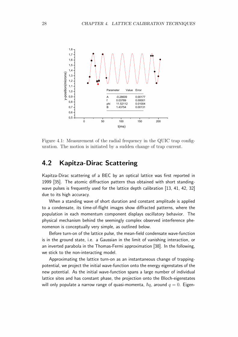
the axial (horizontal) direction, and 37.9 Hz in radial directions (see Fig. 4.1).
Along the vertical direction a lattice is formed by a λ = 914 nm retro-reflected
laser beam with a 1/e2 waist of 120 µm. After a variable interaction time ∆t,
the condensate is released and images are taken after time-of-flight.
27
28 CHAPTER 4. LATTICE CALIBRATION TECHNIQUES
0 50 100 150 2000,5
0,6
0,7
0,8
0,9
1,0
1,1
1,2
1,3
1,4
1,5
1,6
1,7
1,8
Parameter Value Error----------------------------------------A -0.28609 0.00177f 0.03789 0.00001phi 11.52112 0.01004B 1.43754 0.00131----------------------------------------
y-po
sitio
n(microns
)
t(ms)
Figure 4.1: Measurement of the radial frequency in the QUIC trap config-uration. The motion is initiated by a sudden change of trap current.
4.2 Kapitza-Dirac Scattering
Kapitza-Dirac scattering of a BEC by an optical lattice was first reported in
1999 [35]. The atomic diffraction pattern thus obtained with short standing-
wave pulses is frequently used for the lattice depth calibration [13, 41, 42, 32]
due to its high accuracy.
When a standing wave of short duration and constant amplitude is applied
to a condensate, its time-of-flight images show diffracted patterns, where the
population in each momentum component displays oscillatory behavior. The
physical mechanism behind the seemingly complex observed interference phe-
nomenon is conceptually very simple, as outlined below.
Before turn-on of the lattice pulse, the mean-field condensate wave-function
is in the ground state, i.e. a Gaussian in the limit of vanishing interaction, or
an inverted parabola in the Thomas-Fermi approximation [38]. In the following,
we stick to the non-interacting model.
Approximating the lattice turn-on as an instantaneous change of trapping-
potential, we project the initial wave-function onto the energy eigenstates of the
new potential. As the initial wave-function spans a large number of individual
lattice sites and has constant phase, the projection onto the Bloch-eigenstates
will only populate a narrow range of quasi-momenta, ~q, around q = 0. Eigen-

4.2. KAPITZA-DIRAC SCATTERING 29
states from multiple bands will, however, contribute. Since all of these states
have different energy, the time evolution of the system during the pulse-time,
∆t, is given by phase-factors, exp(−iEm(q ≈ 0)∆t/~) for each component.
At the end of the lattice pulse, the resulting state is projected onto plane
waves, i.e. momentum eigenstates. And as the magnetic trapping potential is
turned off at the same time, the amplitude of the projection onto each of these
plane-wave momentum-eigenstates is directly mapped to the real-space position
by the evolution during time-of-flight. It is important to recognize that each
|m, q ≈ 0⟩ state will project onto multiple pn = 2n~kr states. And, vice versa,
each of the observed pn components will in general contain contributions from
multiple bands, and thus display complex oscillatory behavior corresponding to
the relative phase evolution of the bands.
For shallow lattice-depths and short enough pulse durations, the effect of
the periodic lattice potential is just to modify the phase, but not the amplitude,
of the mean-field wave function. The momentum distribution in this ”thin
grating” limit can be expressed by Bessel functions [35].
For longer, but weak pulses, the momentum distribution is found to display
simple oscillations. In the band-structure picture used here, this is because the
initial projection primarily populates states |m = 0, q ≈ 0⟩ and |m = 2, q ≈ 0⟩,i.e. band 0 and 2, while the first band is not populated due to parity.
For deeper lattices the higher bands become important, and the evolution
of each pn(∆t) component must be calculated numerically. The non-periodic
oscillations of pn(∆t) can thus be used for calibration without any lattice depth
limit, provided that a fast numerical 1D band-structure calculation is used within
in the fit routine.
To examine the deep lattice Kapitza-Dirac scattering experimentally, the
lattice pulse is applied to the BEC for a duration ∆t. The lattice and magnetic
trap are then turned off simultaneously, and the BEC is allowed to expand freely
for 14 ms. After the expansion, we take absorption images showing clearly
separated momentum components pn = 2n~kr.For each scattering order n, we measure the atom number Nn. In figure 4.2
we plot Nn/NT vs ∆t (NT is the summed total atom number) and comparing
with the numerically fitted band-structure calculation (solid curves), we find
that all orders give the same value of the lattice depth, here V0 = 40.8Er.
In this way, we can determine the correspondence between the signal from a
photo-detector probing a sample of the lattice beam, and the actual lattice
depth. The Kapitza-Dirac scattering method is thus a fast and reliable tool for
lattice depth calibration, which covers a broad range of lattice depth regimes.

30 CHAPTER 4. LATTICE CALIBRATION TECHNIQUES
0 10 20 30 40 500.0
0.2
0.4
0.6
0.8
1.0
Time HΜsL
Nor
mal
ized
atom
num
ber
Figure 4.2: Time evolution of each momentum component as a function ofKapitza-Dirac pulse duration (∆t). Blue, red, green, and purple correspondto the momentum order n = 0, 1, 2, 3, and 4, respectively. All momentumcomponents give the same result for the optical lattice depth.
4.3 Bloch Oscillation and LZ-Tunneling
Coherent splitting of a condensate by Landau-Zener (LZ) tunneling can occur
when matter waves are accelerated in an optical lattice, and Bloch oscillation of
the non-tunneling fraction even allows multiple consecutive splittings to occur
at regular intervals [3]. Morsch et al. [30] loaded BECs of rubidium atoms
into a shallow optical lattice that was subsequently accelerated by chirping the
frequency difference between the lattice beams. From the resulting interference
pattern, the condensate group velocity in the frame of reference of the lattice
was calculated and plotted against the lattice velocity, clearly showing the Bloch
oscillations. They also demonstrated LZ tunneling as a tool for measuring the
optical lattice depth as well as the effects of the mean-field interaction between
the atoms in the condensate [10]. Recently, Bloch oscillations of condensates in
a vertical lattice are being used in the context of atom interferometry [17, 22].

4.3. BLOCH OSCILLATION AND LZ-TUNNELING 31
4.3.1 Bloch Oscillation
When a matter-wave packet with narrow quasi-momentum distribution around
q(t) is subjected to a constant uniform external force, the quasi-momentum will
increase similarly to the momentum of a free particle. In the case of gravitational
acceleration, g, of an atom with mass m, the quasi-momentum is thus [31]
~q(t) = ~q0 +mgt (4.1)
At the edge of the Brillouin-zone (q = kr), the periodic lattice potential
fulfills the condition for Bragg-reflection of the wave-packet into q = −kr. In
the band-structure picture, one may think of the same physical process as an
adiabatic following at the avoided crossing of the bands. For vanishing lattice
depth, the band-structure is identical to the free-particle dispersion curve, and
there is no energy-gap between any of the bands crossing at q = ±kr (or at
q = 0 for higher bands). For increasing lattice depth, however, avoided crossings
of the energy-bands appear. The lowest band-gap can be seen clearly in figure
3.1, while the higher band-gaps open at increasing lattice depths. For increasing
gap width compared to the acceleration, the probability that the particle will
make an adiabatic ”jump” from one band to another, instead of continuing the
Bloch cycle in the same band, diminishes.
4.3.2 Landau-Zener Theory
To analyze the transition probability between the bands, an approximative time-
dependent Hamiltonian description can be used. One of the few exactly solvable
systems involving time-dependent Hamiltonians is the classic two-level crossing
Landau-Zener problem,
H(t) =~2
(αt Ω
Ω −αt
)(4.2)
where α and Ω are real constants. For small band-gaps, this models the avoided
crossings occurring in the band-structure picture, while for larger gaps, the non-
linearity of the bands becomes significant.
The Hamiltonian (4.2) is defined in the diabatic basis, whose energy eigen-
values cross for Ω = 0, and are given by Ediab = ±~2αt. For Ω = 0, the
time-dependent adiabatic eigenvalues are
Eadiab = ±~2
√Ω2 + α2t2 (4.3)

32 CHAPTER 4. LATTICE CALIBRATION TECHNIQUES
-4 -2 2 4t
-2
-1
1
2
E
Figure 4.3: General form of an avoided two level crossing with adiabaticlevels (solid) and diabatic levels (dashed). Dimensionless, Ω = α = ~ = 1.
The avoided crossing of the adiabatic levels, and the crossing diabatic levels are
shown schematically in figure 4.3.
If Ω2/α ≫ 1, i.e. if the system changes slowly or the coupling is large, the
probability of a ”jump” across the avoided crossing gap, from one adiabatic
level to the other, is vanishing. The system state instead follows the adiabatic
curves. In the other limit, Ω2/α ≪ 1, the system will follow the diabatic levels
and jump across the gap.
The probability, p, that a system prepared in a particular adiabatic state
at t = −∞ will make a non-adiabatic transition and be found in the other
adiabatic state (i.e. the same diabatic state) at t = ∞ is [45, 44]
p(∞,−∞) = e−πΩ2/(2α) (4.4)
This simple result can be derived by means of contour integration, without
actually solving the time-dependent Schrodinger equation explicitly [48].
In the context of optical lattice band-structure, the analytical result from
the Landau-Zener model can be used to describe the dynamics of accelerated
lattices.
4.3.3 Experimental Verification of the Landau-Zener Model
To study the splitting by LZ tunneling, we switch off the magnetic trap and let
the atoms evolve in the combined lattice and gravitational potential. Ideally
this should map a large part of the wave-function onto the q ≈ 0 states of the
lowest band, which would then undergo quasi-momentum evolution as described
above. In reality, some practical problems occur.
While turning off the magnetic QUIC-trap, induced currents in chamber
walls and other nearby metallic objects can have a significant influence on the

4.3. BLOCH OSCILLATION AND LZ-TUNNELING 33
0. 0.5 1. 1.5 2. 2.50.0
0.2
0.4
0.6
0.8
1.0
Lattice depth HEr L
Tun
nelin
gpr
obab
ility
Figure 4.4: Landau-Zener tunneling between the two lowest energy bandsof a condensate in an optical lattice as a function of the lattice depth. Theblue solid line is the curve from Eq. (4.6) and the dots correspond to theexperimental images shown below in (a)-(f)
magnetic field gradient at the trap center. In particular, there may be an
asymmetry between the currents induced in metallic objects near the upper and
lower quadrupole coil, respectively, as witnessed by the following example:
Few cm above the upper QP-coil in the QUIC trap, there is an aluminum
bread-board with a hole for the vertical imaging and lattice light. The board was
installed when implementing the optical lattices, but it soon became apparent
that it would act as a low-resistance inductive circuit with a calculated time-
constant of several milliseconds. Due to its placement close to the upper QP-
coil, the inductive coupling was strong, and experimentally it was found to
impart a large Zeeman-broadening on the optical transition used for imaging,
even in 10 ms time of flight experiments. An easy, and sufficient, solution was

34 CHAPTER 4. LATTICE CALIBRATION TECHNIQUES
to cut a slit in the bread-board to open the loop-circuit.
In the current setup, the temporary field asymmetry during QUIC turnoff
seems to be the opposite: A small but significant upward momentum-kick results
from the trap turnoff. The interpretation is that induced currents in the vicinity
of the lower QP-coil create a gradient in the B-field amplitude, which in turn
accelerate the atoms very briefly in the upward direction. In order to load the
trapped condensate wave-function into the lowest lattice-band, one can thus
either wait until the vertical momentum of the released condensate becomes
zero, before (semi-adiabatically) ramping up the lattice power. Or, alternatively,
turn on the lattice adiabatically while still in the magnetic QUIC trap, and use
a sufficient lattice-depth to suppress any LZ tunneling out of the lowest band
during the QUIC turnoff.
The experiments presented in the next chapter use the former method, while
here the latter approach is used with an initial lattice depth of 2.4 Er. In this
way we initiate well defined Bloch oscillations in the lowest band. The period
of the oscillation is given by
τB =2~krmg
(4.5)
where g is the gravitational acceleration and m is the 87Rb mass, resulting in
τB close to 1 ms.
If the condensate is subjected to the acceleration a and crosses the band gap
∆ at the Brillouin-zone edge, the analytical tunneling probability from LZ-theory
is
r = exp(−ac
a
)= exp
(− λ∆2
8~2a
)(4.6)
where ac is the critical acceleration and a is gravitational acceleration in our
experiment.
During the first Bloch oscillation period, the lattice depth is ramped down,
so that a chosen fraction of the condensate tunnels to the second band when
the quasi-momentum reaches the edge of the Brillouin-zone. Since higher band-
gaps are much narrower, the atoms that tunnel to the second band are essentially
free, and can be seen as the lower components in Fig. 4.4 (a) to (f).
The other fraction is Bragg reflected as described above. During the next
1 ms Bloch period, the lattice is then ramped down completely, releasing also
the reflected fraction. These atoms are visible as the upper components in
figure 4.4 (a) to (f).
The tunneling propability is measured directly from the number-ratio of the
split condensates, rather than measuring the number of atoms that remain
trapped after some multiple of the Bloch period τB [10]. We find that with

4.4. LATTICE MODULATION 35
the lattice depth independently calibrated using Kapitza-Dirac scattering, the
observed splitting ratio is in good agreement with LZ theory, as shown by the
solid curve in figure 4.4.
4.4 Lattice Modulation
A third method of measuring the lattice depth is by direct modulation of the
lattice amplitude. This method is only useful in a regime where the lattice is
deep enough to support atoms against gravity in both band 0 and band 2.
After loading the BEC into the optical lattice, the magnetic trap is turned
off. The lattice amplitude is modulated to excite the atoms from the lowest
band (band 0) to the second excited band (band 2) for a time scale of a few
milliseconds. A set of images are taken in a certain time after the modulation
is finished. Deep lattice depths leads to the regime of 2D pancake shaped
condensates where tunneling between adjacent lattice sites is suppressed. In
this case, the images of the atomic cloud in the optical lattice are taken at
various holding times which show that the atoms are trapped in the lattice
against gravity. Even though the lattice depth is deep enough to hold atoms in
both bands, a small fraction are heated to even higher bands by the modulation,
and fall out of the lattice by tunneling.
For the purpose of detecting the population in the excited band, the mag-
netic and the lattice potential are switched off to perform time-of-flight experi-
ments. By making the lattice turn-off an adiabatic ramp (while still taking less
than τB), the second band population is mapped to the p = ~(q ± 2kr) mo-
mentum components, and can thus be separated from the band 0 population,
which map to p = ~q under time-of-flight. Plotting the relative population in
each band as a function of the modulation frequency gives a narrow resonance
peak, as shown in figure 4.5.
4.5 Summary
Three different methods of lattice depth calibration has been investigated, and
their practical use demonstrated. Each method has both advantages and disad-
vantages, however, and the choice between the three thus depends on several
parameters.
Both the Landau-Zener tunneling method and the lattice modulation method
gives data which can easily be interpreted. For the lattice modulation, the curve
of potential depth versus resonant modulation frequency is sufficient to inter-

36 CHAPTER 4. LATTICE CALIBRATION TECHNIQUES
0 20 40 60 80 1000.0
0.1
0.2
0.3
0.4
Modulation frequency HkHzL
Pop
ulat
ion
inex
cite
dba
ndsHa
.u.L
at 58.4 kHz
0 20 40 60 80 1000
20
40
60
Modulation frequency HkHzL
Pot
entia
ldep
thHE
rL
Figure 4.5: The atoms are excited by modulating the depth of the opticallattice, and the population in the excited band is measured by adiabaticallymapping the atoms in each band to the free particle momentum space (seetext). The narrow resonance at 58.4 kHz comes from the energy differencebetween band 0 and band 2, corresponding to a lattice potential with adepth of 38.7 Er (blue solid curve in the inset). The insert displays the dis-crepancy between the harmonic oscillator level-splitting (red dashed curvein the inset) and the calculated distance at q = 0 between band 0 and 2(blue curve in the inset)
pret the results. One should, however, be cautious that the implementation of
lattice modulation used here assumes that the widths of both band 0 and 2 are
negligible. The method is thus primarily useful for large lattice depths. Another
complication is that it can take a long time to find the resonance to begin with,
if no good initial guess exists.
Lattice calibration by Landau-Zener tunneling also gives a fairly simple anal-
ysis of the experimental data. The critical acceleration ac can be extracted
from the observed splitting ratio r and the known acceleration a, and compared
with tabulated values from a 1D band-structure calculation. When using only
the gravitational acceleration, however, it covers just a narrow range of lattice
depths. This limits its practical usefulness in our current setup.
The Kapitza-Dirac method, with a 1D bandstructure calculation being called

4.5. SUMMARY 37
repeatedly in the loop of a numerical fitting algorithm, is more involved in terms
of data-analysis than the other methods. Once implemented in the lab routines,
however, a clear advantage is that it applies to a much broader range of lattice
depths, and is experimentally straight forward.


Chapter 5
Dynamically Controlled Lattices
The main results of this chapter are to be published in [36].
5.1 Introduction
This chapter reports on the splitting of a BEC in the presence of a time-
dependent optical lattice potential. First we demonstrate that a matter wave
packet can be divided into a set of discrete momentum components, whose
number and fractions can be precisely controlled using a time-dependent lattice
depth. Next we study an atomic Bose-Einstein condensate, which is set in mo-
tion by displacing the magnetic trap, in the presence of time-dependent optical
Bragg mirrors. We demonstrate high-order Bragg reflection of the oscillating
condensate due to multi-photon Raman transitions, and we demonstrate the ini-
tial steps toward realizing a recombination of a split condensate in a harmonic
trap.
5.2 Overview
Two distinct scenarios are investigated. In a first experiment we initiate Bloch
oscillations in a vertical lattice under the constant force of gravity. Time-
dependent control of the Landau-Zener tunneling rate enables us to realize a
controlled matter wave beam splitter and a coherent matter wave source with
controlled output coupler.
In a second experiment we investigate the coherent splitting of a Bose-
Einstein condensate with an optical lattice in the presence of an external mag-
39

40 CHAPTER 5. DYNAMICALLY CONTROLLED LATTICES
netic trapping potential. This allows us to investigate a matter wave splitter
based on high-order Bragg reflection. Finally, time dependent first order Bragg-
mirrors in a harmonic trap demonstrate multiple splittings of a condensate.
The dynamics of a condensate in an optical lattice is governed by the band
structure of the periodic potential. The quadratic energy spectrum of a free
particle splits up into bands which are labeled by the eigenenergies En(q) with
the eigenstates |n, q⟩, where n denotes the band index and q the atomic quasi-
momentum, as described in chapter 3. The bands are separated by energy gaps
whose size depends on the lattice depth as shown in Fig. 5.3. As a consequence
the dynamics of an atom moving in such a potential is dramatically altered.
If an atom is subject to a force along the lattice axis, the band structure
causes the atom to start oscillating instead of being constantly accelerated.
These so-called Bloch oscillations occur, since an atom is Bragg reflected as
it approaches the edge of the Brillouin zone. The Bloch period is given by
τB = 2~kr/(ma), where kr = 2π/λLat, m is the atomic mass, and a is the
acceleration. The Bloch period corresponds to the time it takes for the atoms
to be accelerated from one end of the Brillouin zone to the other. If the lattice
beams are arranged to create a periodic potential along the vertical direction, a
condensate can be held against gravity for several seconds in a sufficiently deep
lattice potential, while the atoms perform Bloch oscillations.
When the lattice potential is reduced and the band gap narrows, Landau-
Zener tunneling between Bloch bands starts to occur. In this regime the tunnel-
ing probability can be calculated from Landau-Zener theory. If the condensate is
moving with acceleration a through the avoided crossing region of the En−1(q)
and En(q) bands, the tunneling probability can be approximated by
Pt(n) = exp(−ac
a
)= exp
(− π∆2
n
4nkra~2
)(5.1)
[13] where we give the generalized expression for tunneling between bands n
and n − 1 for future reference. Here ac is the critical acceleration, ∆n is size
of the band gap at the quasimomentum n~kr, and a is the acceleration of the
atoms with respect to the lattice rest frame. In the experiments described in
Sec. 5.3, the acceleration a is determined by gravity, while in Sec. 5.4 a is
related to the slope of the harmonic potential at the instantaneous position of
the atoms. The generalization to n > 1 follows from section 4.3.2 by noting
that α in equation 4.4 is linear in n.
Since the experiments are carried out with ensembles of particles, their in-
teraction modifies the single particle band structure outlined above. This effect
is most pronounced at the edge of the Brillouin zone and can be described by

5.3. CONTROLLED MATTER WAVE BEAM SPLITTER 41
a mean-field nonlinearity that causes a modification of the tunneling behavior.
The tunneling rates in two directions between the Bloch bands also become
different [24]. This work, however, is restricted to the weak interaction regime,
where the tunneling probability is well approximated by the Landau-Zener for-
mula. Experimentally the tunneling probability is set by controlling the optical
lattice depth and can be suppressed completely when the lattice depth is in-
creased.
5.3 Controlled Matter Wave Beam Splitter
In a first set of experiments we demonstrate that time-dependent control of
the Landau-Zener tunneling rate enables us to realize a controlled matter wave
beam splitter and output coupler.
To initiate the splitting mechanism, the magnetic trap is suddenly switched
off and the atoms evolve in the combined lattice and gravitational potential.
The atoms start to perform Bloch oscillations and each time they reach the
edge of the Brillouin zone a fraction of the atoms can tunnel to a higher band.
If the lattice depth is chosen such that atoms in higher bands with n ≥ 1 are
not bound, these atoms start to fall under the influence of gravity. Thus the
condensate is split each time the edge of the Brillouin zone is encountered and
atoms with n ≥ 1 fall out of the lattice while Bragg reflected atoms remain
trapped. If the tunneling probability Pt(n) is held fixed and the initial atom
number is N0 the number of atom tunneling out of the lattice on the m’th
Bloch period is N0(1 − Pt(1))m−1Pt(1) and N0(1 − Pt(1))
m atoms remain
in the lattice. This mechanism was indeed used within the first experiments
with Bose-Einstein condensates in optical lattices [3] and later investigated in
detail [30, 10, 24].
Alternatively however, the dynamical control available in experiments with
optical lattices can be used to enhance this static situation. If the lattice depth
is controlled synchronously with the Bloch oscillation period, the tunneling rate
can be controlled individually for each tunneling event and thus the fraction of
outcoupled atoms can be determined at will for each Bloch cycle.
Within our experiments the following sequence is used to realize this beam
splitter. After production of a Bose-Einstein condensate the magnetic trap is
switched off to release the atoms. Within this process the atoms receive a small
initial upwards velocity of 9mm/s and hence reach q = 0 after 920µs due to
gravity.
The Bloch oscillations are initiated by turning on the lattice at a depth suf-
42 CHAPTER 5. DYNAMICALLY CONTROLLED LATTICES
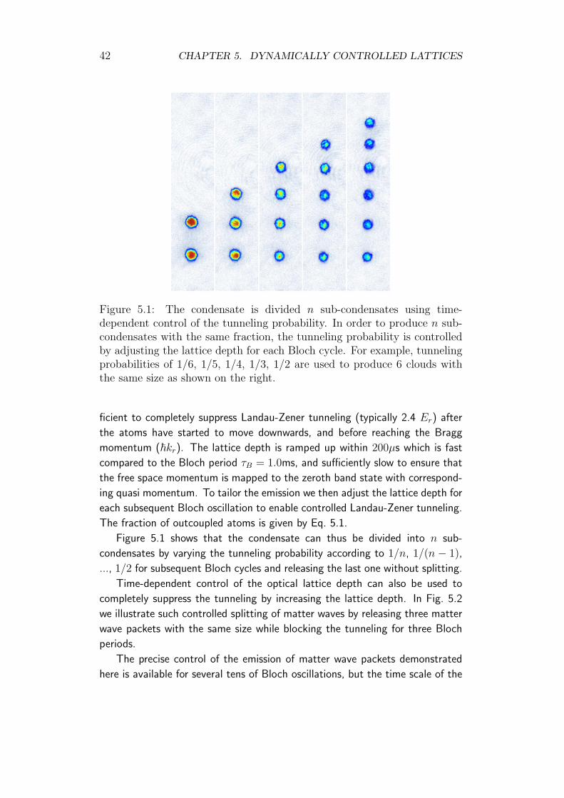
Figure 5.1: The condensate is divided n sub-condensates using time-dependent control of the tunneling probability. In order to produce n sub-condensates with the same fraction, the tunneling probability is controlledby adjusting the lattice depth for each Bloch cycle. For example, tunnelingprobabilities of 1/6, 1/5, 1/4, 1/3, 1/2 are used to produce 6 clouds withthe same size as shown on the right.
ficient to completely suppress Landau-Zener tunneling (typically 2.4 Er) after
the atoms have started to move downwards, and before reaching the Bragg
momentum (~kr). The lattice depth is ramped up within 200µs which is fast
compared to the Bloch period τB = 1.0ms, and sufficiently slow to ensure that
the free space momentum is mapped to the zeroth band state with correspond-
ing quasi momentum. To tailor the emission we then adjust the lattice depth for
each subsequent Bloch oscillation to enable controlled Landau-Zener tunneling.
The fraction of outcoupled atoms is given by Eq. 5.1.
Figure 5.1 shows that the condensate can thus be divided into n sub-
condensates by varying the tunneling probability according to 1/n, 1/(n − 1),
..., 1/2 for subsequent Bloch cycles and releasing the last one without splitting.
Time-dependent control of the optical lattice depth can also be used to
completely suppress the tunneling by increasing the lattice depth. In Fig. 5.2
we illustrate such controlled splitting of matter waves by releasing three matter
wave packets with the same size while blocking the tunneling for three Bloch
periods.
The precise control of the emission of matter wave packets demonstrated
here is available for several tens of Bloch oscillations, but the time scale of the
5.4. MATTER WAVE SPLITTING IN HARMONIC TRAP 43
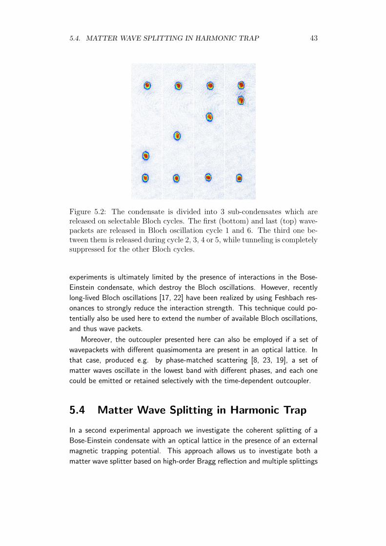
Figure 5.2: The condensate is divided into 3 sub-condensates which arereleased on selectable Bloch cycles. The first (bottom) and last (top) wave-packets are released in Bloch oscillation cycle 1 and 6. The third one be-tween them is released during cycle 2, 3, 4 or 5, while tunneling is completelysuppressed for the other Bloch cycles.
experiments is ultimately limited by the presence of interactions in the Bose-
Einstein condensate, which destroy the Bloch oscillations. However, recently
long-lived Bloch oscillations [17, 22] have been realized by using Feshbach res-
onances to strongly reduce the interaction strength. This technique could po-
tentially also be used here to extend the number of available Bloch oscillations,
and thus wave packets.
Moreover, the outcoupler presented here can also be employed if a set of
wavepackets with different quasimomenta are present in an optical lattice. In
that case, produced e.g. by phase-matched scattering [8, 23, 19], a set of
matter waves oscillate in the lowest band with different phases, and each one
could be emitted or retained selectively with the time-dependent outcoupler.
5.4 Matter Wave Splitting in Harmonic Trap
In a second experimental approach we investigate the coherent splitting of a
Bose-Einstein condensate with an optical lattice in the presence of an external
magnetic trapping potential. This approach allows us to investigate both a
matter wave splitter based on high-order Bragg reflection and multiple splittings

44 CHAPTER 5. DYNAMICALLY CONTROLLED LATTICES
of a matter wave.
To induce motion, the minimum of the combined gravitational and magnetic
potential is suddenly shifted in the y direction (the vertical axis) by increasing
the current to the QUIC coils (from 150 A to 200 A). After this displacement, the
BEC undergoes harmonic motion with an amplitude of 89.6 µm and oscillation
period T = 19.5 ms. For future reference we define the first and second turning
points at t = T/2 and t = T as P1 and P2, respectively. In the experiment,
we focus on the Bragg reflection and Landau-Zener tunneling of a BEC as it
is accelerating and decelerating in the external potential. After triggering the
harmonic motion in the magnetic trap, an optical lattice potential along the
y-axis is briefly applied to the BEC at different times to induce the controlled
splitting.
We have previously discussed the dynamics of a BEC initially at rest as it
is being accelerated across the band edge. If, on the other hand, a conden-
sate with high initial momentum is decelerated while in a lattice, Landau-Zener
tunneling between higher excited bands and higher order Bragg reflection can
happen depending on the lattice depth (see Fig. 5.3). In the harmonic exter-
nal confinement this occurs as the condensate approaches one of the classical
turning points coming from the trap center.
Bragg scattering for atoms can be described as a multi-photon Raman pro-
cess, in which an atom of initial momentum p = n~kr along the lattice axis is
transferred to a superposition of the initial momentum state and the state with
momentum p = −n~kr. The integer n is the order of the Bragg scattering,
and obviously 2n photons are exchanged for each scattered atom.
Let us consider an atom moving from higher to lower bands. Remember
that in the overall harmonic external confinement this means that in position
space the atoms are approaching one of the turning points. As illustrated in
Fig. 5.3, even the higher band-gaps open at sufficiently large lattice depths,
which means that different orders of Bragg reflection can occur at the avoided
crossings.
We denote the partially reflecting Bragg mirror at the transition from band
n to band n − 1 by BMn. For example, for the potential depth of 4.6 Er,
Fig. 5.3 (middle) shows how part of the condensate is Bragg reflected on BM2
in a 4-photon process. If the lattice is kept on, the transmitted (and thus still
decelerating) fraction will subsequently reach BM1, where it is fully reflected. In
real space this corresponds to the second-order Bragg reflected part of the cloud
reversing direction of propagation, whereas the unreflected part continues being
decelerated until it is first-order Bragg reflected without reaching the classical
turning point.
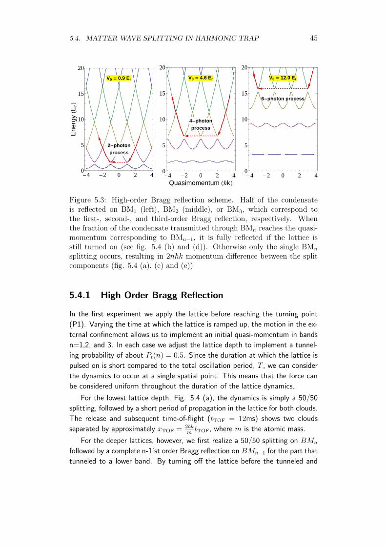
5.4. MATTER WAVE SPLITTING IN HARMONIC TRAP 45
V0 = 0.9 Er
2-photonprocess
-4 -2 0 2 40
5
10
15
20E
nerg
yHE
rLV0 = 4.6 Er
4-photonprocess
-4 -2 0 2 40
5
10
15
20
Quasimomentum HÑkL
V0 = 12.0 Er
6-photon process
-4 -2 0 2 40
5
10
15
20
Figure 5.3: High-order Bragg reflection scheme. Half of the condensateis reflected on BM1 (left), BM2 (middle), or BM3, which correspond tothe first-, second-, and third-order Bragg reflection, respectively. Whenthe fraction of the condensate transmitted through BMn reaches the quasi-momentum corresponding to BMn−1, it is fully reflected if the lattice isstill turned on (see fig. 5.4 (b) and (d)). Otherwise only the single BMn
splitting occurs, resulting in 2n~k momentum difference between the splitcomponents (fig. 5.4 (a), (c) and (e))
5.4.1 High Order Bragg Reflection
In the first experiment we apply the lattice before reaching the turning point
(P1). Varying the time at which the lattice is ramped up, the motion in the ex-
ternal confinement allows us to implement an initial quasi-momentum in bands
n=1,2, and 3. In each case we adjust the lattice depth to implement a tunnel-
ing probability of about Pt(n) = 0.5. Since the duration at which the lattice is
pulsed on is short compared to the total oscillation period, T , we can consider
the dynamics to occur at a single spatial point. This means that the force can
be considered uniform throughout the duration of the lattice dynamics.
For the lowest lattice depth, Fig. 5.4 (a), the dynamics is simply a 50/50
splitting, followed by a short period of propagation in the lattice for both clouds.
The release and subsequent time-of-flight (tTOF = 12ms) shows two clouds
separated by approximately xTOF = 2~kmtTOF, where m is the atomic mass.
For the deeper lattices, however, we first realize a 50/50 splitting on BMn
followed by a complete n-1’st order Bragg reflection on BMn−1 for the part that
tunneled to a lower band. By turning off the lattice before the tunneled and

46 CHAPTER 5. DYNAMICALLY CONTROLLED LATTICES
HaL HbL HcL HdL HeL
Figure 5.4: Time-of-flight images. The condensate is split by the interactionwith optical lattices with the depth of (a) 1.1 Er, (b) and (c) 5.0 Er, (d) and(e) 13.5 Er. The upper cloud in (a), (c), and (e) is the fraction without anyreflection, and the lower cloud in all images is the one reflected from BMn,i.e. BM1 for (a), BM2 for (b) and (c), BM3 for (d) and (e). The upper cloudsof (b) and (d) have been transmitted on BMn and subsequently reflectedon BMn−1.
reflected part comes back to the BMn mirror, we expect two peaks separated
by xTOF but shifted by (n−1)xTOF relative to the BM1 case. This can be seen
in Fig. 5.4 (b) and (d).
The second, full Bragg reflection can be avoided by turning off the lattice
before q = (n− 1)~k is reached. In this case, as illustrated in Fig. 5.4 (c) and
(e), we get a cloud unaffected by the lattice and one shifted by nxTOF.
This series of matter wave splittings demonstrates a large momentum trans-
fer beam splitter [9, 13]. Our experiments thus show that higher-order Bragg
reflections can be manipulated by controlling the lattice depth and pulse timing.
5.4.2 Recombination of Split Clouds
An interesting application of the beam splitting process would be to utilize the
harmonic confinement to recombine parts of the cloud that have been split
earlier. We investigate this by pulsing on Bragg mirrors in the vicinity of both
turning points (P1 and P2) in the harmonic trap (see Fig. 5.5).

5.4. MATTER WAVE SPLITTING IN HARMONIC TRAP 47
0 0.2 0.4 0.6 0.8 1 1.2 1.4−1
−0.8
−0.6
−0.4
−0.2
0
0.2
0.4
0.6
0.8
1
t/T
y po
sitio
n (a
.u.)
Figure 5.5: Principle of the recombination experiment. Blue curves showspatial harmonic oscillation of the condensate in the harmonic confinement,while the red lines schematically indicate the positions where the 50/50BM1 mirrors split the condensate. In the experiment of Fig. 5.6 (b), onlythe first Bragg mirror pulse is used, while in Fig. 5.6 (c), both are used.
Figure 5.6 (a) shows the condensate after the first two turning points (P1
and P2) without an optical lattice. A Bragg mirror (BM1) with tunneling
probability of 0.5 and duration less than one Bloch period is pulsed on briefly
before the condensate reaches the turning point P1 to produce two equally split
condensates with 2~kr initial momentum difference. The split wave-packets are
reflected at the classical turning points P1 and P2, and then the images are
grabbed after turning off the magnetic field and time-of-flight (Fig. 5.6 (b)).
In addition to the intended vertical oscillatory motion, a significant difference
in transverse position between the Bragg-reflected and transmitted clouds is
evident. The origin of this transverse motion is currently being investigated.
In order to recombine the split clouds, we apply a 2nd Bragg pulse in the
vicinity of the second turning point, P2, at the time when the two clouds
are (ideally) spatially overlapped but with opposite momenta (see figure 5.5).
The Bragg reflected part of the first cloud now has the same momentum as the
transmitted part of the second and vice versa. Figure 5.6 (c) is the time-of-flight
image taken when turning off the magnetic field 2 ms after passing the second
turning point P2. As can be seen, unfortunately the transverse movement is so
large that the recombined clouds are not spatially overlapped and therefore no

48 CHAPTER 5. DYNAMICALLY CONTROLLED LATTICES
HaL HbL HcL
Figure 5.6: Images (a), (b), and (c) are taken at t = 48 ms, and trap isturned off at 21.5 ms, i.e. right after the second turning point, where mo-mentum difference is large (see Fig. 5.5). (a) The BEC undergoes harmonicmotion in magnetic trap potential without lattice light. (b) The BEC issplit into two clouds by the Bragg mirror (BM1) at P1. The two clouds arenot on a vertical line (y axis) due to undesired motion along the z direction.(c) The split clouds are split again from the Bragg mirror (BM1) at P2.
interference effects can be observed.
5.5 Summary
In summary, we have demonstrated high contrast coherent matter wave packet
splitting using time-dependent control of the intensity of standing light waves.
In this way the tunneling probability in each Bloch oscillation period was ad-
justed to control the outcoupled fraction dynamically, and even suppress tun-
neling completely.
We have furthermore demonstrated the dynamics of a BEC in a combined
potential consisting of a magnetic trap and an optical lattice. We initiated BEC
motion by suddenly displacing the magnetic trap, and used this to demonstrate
high-order Bragg reflection. Finally, we have used two distinct Bragg-mirror
pulses close to the classical turning points in a harmonic trap to (almost) im-
plement a matter-wave Mach-Zender interferometer, which unfortunately so far
is misaligned due to transverse motion in the trap.

Chapter 6
Quasi-Continuum Wavepacket
Coupling to Localized States
The main results of this chapter are to be published in [27].
6.1 Introduction
In the preceding chapters dealing with single-particle bandstructure dynam-
ics like Kapitza-Dirac scattering, Bloch-oscillation and Landau-Zener tunneling,
the primary experimental detection technique has been time-of-flight imaging.
Some of the described mechanisms, e.g. Bloch-oscillation, also display char-
acteristic behavior in position-space, which could be probed directly. It might
thus seem obvious to also image the condensate dynamics in direct space, rather
than to map the reciprocal space using time-of-flight.
However, it is not obvious that such an approach could also provide useful
results for condensates held in a combined lattice and magnetic trap. The
tight magnetic confinement normally used during the evaporative cooling yields
condensates that are barely resolvable with our imaging setup. And since the
absorption-imaging beams are close to resonance, both the extraordinarily high
in-trap optical density of the condensates, and the Zeeman-shifts due to the
trap B-field, would seem to be prohibitively complicating factors, making time-
of-flight imaging a better option.
By using weak magnetic confinement together with a 1D optical lattice
with the option of amplitude modulation, in-trap imaging of condensates was,
however, found experimentally to give very intriguing results. Both localized
49

50CHAPTER 6. QUASI-CONTINUUM WAVEPACKET COUPLING TO
LOCALIZED STATES
stationary states [34] and states displaying moving wave-packet characteristics
was observed in-trap. This chapter presents some of the recent data and results
that have so far come out of the investigation.
6.2 Experimental Setup
Following the evaporative cooling and BEC creation, the QUIC trap is relaxed
to 12.3 and 37.9 Hz trapping frequencies in the axial and radial directions,
respectively.
An optical lattice with a depth of typically 16Er is adiabatically turned
on to load the BEC into the (mean-field) groundstate of the combined QUIC
and lattice potential. The lattice is intensity-modulated (5-20% peak-to-peak
amplitude) with a frequency ν for a variable time-span, (0.5-10 ms). After a
variable hold-time, absorption images are taken in-trap.
6.3 Stationary Localized Atoms
Using a 10 ms modulation pulse, the in-trap images display patterns of ”outly-
ing” atomic clouds of varying optical density (see Fig. 6.1 and 6.2).
By varying the hold-time between modulation and imaging, the outlying
clouds are found to be stationary, and they survive a complete turn-off of the
magnetic trapping potential (see Fig. 6.3). The QUIC turn-off removes the
diffuse cloud of quasi-continuum atoms visible between the central BEC and
the outlying clouds, but leaves the positions of the peaks unchanged.
Figure 6.4 shows how diagonalization of the 1D Schrodinger equation with
our trap potential leads to both localized and various degrees of delocalized
eigenstates, which can explain the observed stationary states [34]. Figure 6.4
also shows clear similarities with the band-structure of periodic lattices, with
”bands” 0, 1 and 2 below, and bands ≥ 3 in the quasi-continuum.
The numerical diagonalization of the symmetric 1D potential leads to solu-
tions which are ±1 eigenstates of parity. A particular eigenstate thus typically
has a component localized on both the left and right flanks of a particular band.
Moving away from the bottom of the band, however, the P = ±1 eigenstates
form perfectly degenerate pairs. Physically this means that even though an
atom initially localized on one flank is described as a coherent superposition of
two split eigenstates, it will, due to the degeneracy, not tunnel from one side
to the other.

6.3. STATIONARY LOCALIZED ATOMS 51
#26, ν=34
20 40
20
40
60
#27, ν=35 #28, ν=36 #29, ν=37 #30, ν=38 #31, ν=30
#32, ν=30.5 #33, ν=31 #34, ν=31.5 #36, ν=32.5 #37, ν=33 #38, ν=33.5
#39, ν=34 #40, ν=34.5 #41, ν=35 #43, ν=36 #44, ν=36.5 #45, ν=37
#46, ν=37.5 #47, ν=38 #48, ν=38.5 #49, ν=39 #50, ν=39.5 #51, ν=35.5
#52, ν=35.5 #53, ν=35.5 #54, ν=35.5 #55, ν=36 #56, ν=37 #57, ν=37.5
#58, ν=38 #59, ν=38 #60, ν=38.5 #61, ν=39 #62, ν=39.5 #63, ν=40
Figure 6.1: In-trap images of condensate and outlying peaks for differentmodulation frequencies. Image sizes are 40 × 70 pixels (square pixels, size(1.94µm)2).

52CHAPTER 6. QUASI-CONTINUUM WAVEPACKET COUPLING TO
LOCALIZED STATES
#86, ν=42
20 40
20
40
60
80
100
#87, ν=43 #88, ν=44 #89, ν=45 #90, ν=46
#91, ν=47 #92, ν=48 #93, ν=49 #97, ν=50 #98, ν=52
#99, ν=53 #100, ν=54 #101, ν=55 #102, ν=56 #103, ν=57
#104, ν=58 #105, ν=59 #106, ν=60 #107, ν=61 #108, ν=62
#109, ν=63 #110, ν=64 #111, ν=65 #112, ν=66 #113, ν=67
2010\week#43\2010−10−27\026_inSitu\plotallImContinuum.m
Figure 6.2: In-trap images of condensate and outlying peaks for differentmodulation frequencies. Image sizes are 40× 100 pixels (square pixels, size(1.94µm)2).

6.4. LOCAL TILTED BAND-STRUCTURE PICTURE 53
HAL
50 Μm
50 Μm
HBL
Figure 6.3: Outlying stationary clouds and central BEC imaged in super-imposed vertical lattice and magnetic trap (A), and with the magnetic trapturned off during the hold-time (B). Both central BEC and outlying statesare seen to be trapped by the lattice alone in (B).
6.4 Local Tilted Band-Structure Picture
Numerical diagonalization of the 1D Schrodinger equation into localized eigen-
states gives an adequate description of the experimentally observed properties
of the stationary states in the combined potential. The physical mechanisms
involved can, however, be illuminated by a local tilted band-structure picture.
This allows for an intuitive understanding of the transition between figure 6.3
(A) and (B), and connects nicely with the previous chapters. While less rigorous,
this approach also helps in the interpretation of the non-stationary wave packets
described below. Fundamentally, however, it is only a different perspective on
the same physics.
The combination of the magnetic and lattice potentials is not periodic, since
the harmonic confinement destroys the 1D periodicity of the lattice. The con-
cepts of Bloch-oscillation and Landau-Zener tunneling can, however, still be
applied here, due to the scale-difference between the relevant magnetic trap
dynamics and the lattice spacing. A qualitative, if not quantitative, under-
standing of the experiments presented below can thus be gained by considering
the harmonic confinement of the magnetic trap to be a ”locally linear tilt” of
the lattice. Wave-packets of narrow quasi-momentum distribution are thus ac-

54CHAPTER 6. QUASI-CONTINUUM WAVEPACKET COUPLING TO
LOCALIZED STATES
-80 -60 -40 -20 0 20 40 60 800
5
10
15
20
25
y HΛL
Ene
rgyHE
rL
Figure 6.4: Spectrum of the 1D Schrodinger equation with combined co-sine lattice potential VL = s cos(kx)2, s = 18Er, and harmonic confinementVB = 1
2mω2
0x2, ω0 = 2π ·38.4Hz. The lower and upper dotted red lines (and
shading in between) indicates VB and VB + s, while the black to light blueshading of the eigenstate solutions discriminates between localized eigen-states (black) to increasingly delocalized eigenstates (light blue).
celerated and undergo Bloch-oscillation or Landau-Zener tunneling under the
assumption of constant acceleration. To use this picture, the quasi-momentum
distribution cannot be infinitely narrow, however, since the spatial extent of
the wavepacket must also be small compared to the motion in the harmonic
confinement. It is thus a qualitative picture, which should be used with some
care.
Considering the situation in Fig. 6.3 (B) in detail, we see that all 3 peaks are
supported against gravity by the lattice alone. There are at least two mechanism
by which this can occur. One is that the lattice is so deep that site-to-site
tunneling is suppressed on the experimental timescale. The lattice depth used
for Fig. 6.3 is 18Er (in the trap center), which corresponds to a total width of
the zeroth band of ~ω, with ω = 2π ·40Hz. Even in the zeroth band, dynamics
would thus be visible, although quite slow.
The other mechanism is repeated Bragg-reflections on the lattice potential,
i.e. Bloch oscillations. Writing the band-gap, ∆, of equation 5.1 in units of the
recoil energy, the critical acceleration determining if Landau-Zener tunneling

6.5. RF-CUT OF LOCALIZED STATES 55
will occur is
ac =∆
Er
h2π2
8m2λ3(6.1)
i.e. ac = (∆/Er) · 34.3m/sec2. With ∆/Er ≈ 7 for the lowest band-gap and
∆/Er ≈ 4 for the second, LZ-tunneling out of both 0th and 1st band is thus
heavily suppressed, when considering the gravitational acceleration.
If we assume that Bloch-oscillation in some band is the mechanism support-
ing the atoms against gravity at all 3 positions, the Landau-Zener tunneling
(and accompanying loss) out of the given band must be suppressed when the
lattice is tilted due to gravity. And, consequently, the LZ-tunneling will be even
more suppressed for any acceleration smaller than g.
Returning to Fig. 6.3 (A), we can estimate the local acceleration at the
outlier-positions due to the harmonic confinement. With vertical trap frequency
ω = 2π ·37.9Hz, and offset distance d = 50µm, the local acceleration a = ω2d
is 2.8m/s2, which is smaller than the gravitational acceleration. From the
above considerations, the localized stationary states can thus be understood
both in terms of localized eigenstates, and Bloch oscillation. Whether the
Bragg-scattering is a first or higher order Raman-process will depend on the
particular band in which the Bloch-cycle occurs, as described in chapter 5.
6.5 RF-Cut of Localized States
Here we consider the localized states arising with lattice depth s = 16 and
modulation frequency ν = 32 kHz. To confirm experimentally that no tunneling
takes place between the observed stationary states while the magnetic trap is
on, we can apply an ”RF-knife”, which works just like the standard RF forced
evaporative cooling. Sweeping the RF frequency will flip the spin of any atoms
passing through the resonance condition shell defined by hνRF = µBgF |B(r)|.The gravitational sag in the weak magnetic confinement is xsag = g/ω2
0 =
173µm (ω0 = 2π · 37.9Hz). It follows that a downward RF frequency sweep
will flip the spins of the lower localized atoms first, then the central state, until
finally reaching the upper localized state (since even the upper localized state
is below the magnetic minimum in the trap). Figure 6.5 shows this process,
while Fig. 6.6 shows that it is also possible to selectively remove the central
component, while leaving the localized states untouched.
By removing all but the upper localized state, it is possible to do an isolated
lifetime measurement on these atoms while both lattice and harmonic confine-
ment is on. Figure 6.7 shows the result of cutting away all but the upper peak
and waiting for a variable time after the end of the RF-sweep. The initial rapid

56CHAPTER 6. QUASI-CONTINUUM WAVEPACKET COUPLING TO
LOCALIZED STATES
#19, end freq.=0
20 40
10
20
30
40
50
60
70
80
90
100
#28, end freq.=8700 #29, end freq.=8650 #21, end freq.=8600 #30, end freq.=8550
2010\week#44\2010−11−03\021_RF_sweep\plotallImages.m
Figure 6.5: Cutting away lower and central in-trap peak with RF-knife.
decay was initially a surprise. With the approach of section 6.4, however, this
is readily explained by noticing that an (accidentally) spin-flipped fraction of
the upper state will still undergo Bloch-oscillation, and thus be confined in the
vertical lattice direction, provided that the new local acceleration is not too
large. The spin flipped atoms will thus not necessarily be expelled vertically
due to gravity, but may leave the fitted region much slower by ”spilling out”
of the lattice beam sideways. In future RF-cut experiments, it is thus crucial
to check this and, if needed, allow enough time for the atoms to escape before
evaluating if the RF-cut is at the desired depth.
6.6 Band-Categorization of the Stationary States
Although the basic confining mechanism can be understood both from the
localized eigenstates in Fig. 6.4 and from the suppression of LZ-tunneling in
section 6.4, the above experiments have not addressed the question of which
”bands” of Fig. 6.4 are actually involved.
To investigate this, we have mapped out the position of the localized peaks
for a range of modulation frequencies ν. For the pictures in Fig. 6.1, the lattice
depth is set to s = 16, the modulation duration is 10 ms, and the modulation
frequency is varied. Each localized state is observed to move further away for
increasing ν, and for frequencies in the range 36-39 kHz, two distinct localized
peaks are visible on each side. Figure 6.8 shows the fitted distance between the

6.6. BAND-CATEGORIZATION OF THE STATIONARY STATES 57
pic #65
0 50 100 15010
20
30
40
\.m
0 500
50
100
150
Figure 6.6: Cutting away the central peak with RF-knife. All dimensionsin 1.94µm pixels.
central peak and the peaks on the lower side.
The energy of an n’th band localized state with mean distance x to the trap
center will have two distinct components, as can be seen from Fig. 6.4. One is
the potential energy in the harmonic potential at x,
Ev =1
2mω2
0x2 (6.2)
while the other is the mean value of the n’th band-energy, averaged over the
quasimomentum. Choosing E0(q = 0) as the energy reference (it is the initial
state), the 1D bandstructure calculation of chapter 3 gives
E1 = ⟨E1(q)⟩= 18.7 kHz · h
E2 = ⟨E2(q)⟩= 33.4 kHz · h (6.3)
for the chosen lattice depth of 16Er.
To find the expected positions of localized states, we make the assump-
tion that the total energy gained by the localized atoms during the vibrational

58CHAPTER 6. QUASI-CONTINUUM WAVEPACKET COUPLING TO
LOCALIZED STATES
0 50 100 150 200 250 3001000
2000
3000
4000
5000
6000
7000
8000
9000
hold time (ms)
atom
num
ber
Upper peak lifetime
2010\week#27\2010−07−09\36_singlePeakVaryHold\\_.m
nsumnfity
Figure 6.7: Lifetime measurement of the upper localized peak after cuttingaway lower and central states with RF-knife (two different atom number fitmethods ploted). The initial decay is, most likely, the slow escape of spinflipped atoms in the upper peak (see text).
excitation is νh, such that
νh =1
2mω2
0x2 + En (6.4)
for a localized state in band n. This leads to the estimated mean distance from
the trap center
x = 12.7µm ·√
(ν − En/h)/kHz (6.5)
The square-root fits shown along with the points labeled n=1 data (upper
curve) and n=2 data (middle curve) in Fig. 6.8 show very good agreement with
the theoretical estimates from (6.5) and (6.3). We thus conclude that most of
the observed peaks correspond to band 1 and 2 states, while no population has
been detected in the localized band 0 states.
The third curve at the bottom may have an interpretation as classical
turning-points for states in the third band. Since these are not localized
states, the relevant parameter for this interpretation would instead be the energy
E3(q = 0).

6.7. QUASI-CONTINUUM WAVEPACKET EXCITATION 59
28 30 32 34 36 38 40 42 44 46 480
10
20
30
40
50
60
mod. freq (kHz)
low
er p
eak
sepa
ratio
n (u
m)
In situ detection, Vctrl
=1.64, Vmod
=2V
2010\week#43\2010−10−27\026_inSitu\loadData.m
n=1 datay=12.69*sqrt(x+−18.5(2))n=2 datay=12.69*sqrt(x+−33.06(17))continuumy=12.69*sqrt(x+−37.89(13))
Figure 6.8: Fitted positions of the lower outlying peaks as function of latticemodulation frequency ν.
6.7 Quasi-Continuum Wavepacket Excitation
Having identified the stationary states as localized band 1 and 2 eigenstates,
we need investigate the mechanism by which these states are being populated.
Using a large amplitude, short (500µs) lattice modulation at ν = 31 kHz, a set
of non-stationary ”wave-packet” states is observed (see Fig. 6.9). Plotting the
positions of the two wavepackets, shows how they move away from the center
and turn around (Fig. 6.10).
To analyze this behavior in the local tilted bandstructure picture, consider
the 1D bandstructure for the s = 16 lattice, shown in Fig. 6.11. A preliminary
interpretation of the recently observed data is the following: During the 500µs
modulation pulse, a band 4 wave-packet centered around q = 0 (corresponding
to extended quasi-momenta ~q = ±4~kr) is prepared in a two-step excitation.
The transition is clearly off-resonant at the experimentally chosen frequency,
but since the modulation is very strong, power-broadening ensures that the
|n = 4, q ≈ 0⟩ state is populated.
The populated state is interpreted as two counter-propagating wavepackets,
while the 8 photon Raman process, which is the physical origin of the band-

60CHAPTER 6. QUASI-CONTINUUM WAVEPACKET COUPLING TO
LOCALIZED STATES
pic #69
0 10 20 30 40 50 600
50
100
150
2010\week#44\2010−11−02\057_modHoldTime\.m
0 100 2000
20
40
60
80
Figure 6.9: In-trap image showing the two moving ”wavepackets”. Imagetaken at 3ms hold time after a 500µs, ν = 31 kHz vibrational excitationpulse of large amplitude (2.16 V p-p, mean lattice depth set by 1.64 V signalon photo-detectors, corresponding to s = 16).
gap, is neglected. The corresponding ”free particle” initial velocity of the wave-
packets is thus
v =4~krm
(6.6)
= 20.1mm/s
Treating the quasi-momentum ~q as the momentum of a classical particle
moving in a harmonic trap (with ω0 = 2π · 37.9Hz), the times at which the
quasi-momentum passes the avoided crossings at q = nkr, 0 ≤ n < 4 are
tn =arccos
(n4
)ω0
(6.7)
giving t3 = 3.0ms. Subtracting the half the width of the 500µs modula-
tion pulse, the estimated time to observe a (6-photon Raman process) Bragg-
reflection on the avoided crossing between band 3 and 2 in Fig. 6.10, would
thus be at 2.785ms, and at a velocity of 15.1mm/sec. Both of these numbers
agree very well with the data of Fig. 6.10, which cannot be explained by simple
harmonic motion at ω0.

6.8. CONTROLLED PREPARATION OF LOCALIZED STATES 61
1 1.5 2 2.5 3 3.5 4 4.5−30
−20
−10
0
10
20
30
hold time (ms)
peak
pos
ition
(pi
x)
single 500us excitation pulse followed by hold time
2010\week#44\2010−11−02\057_modHoldTime\.m
Figure 6.10: Fitted vertical positions of the two ”wavepackets” (see Fig. 6.9)as a function of hold-time. The turning-point is interpreted as a 6-photonBragg scattering (see text).
6.8 Controlled Preparation of Localized States
The recent results of the preceding section suggests a cleaner way to populate
the localized states, and opens up a wealth of interesting future experimental
possibilities.
Firstly, the range of excitation frequencies that was observed to produce
band 1 localized states in Fig. 6.8 was in the range 30 to 39 kHz. This roughly
corresponds to the range of frequencies in the 2. band, and suggests that the
band 2 states make it possible to populate higher-momentum states in a two
step excitation.
To generate high momentum wave-packets without using excessive ampli-
tude modulation, a possibility is thus to chose a lattice-depth, where the two
steps are both resonant at q = 0. This occurs at approximately s = 14 with an
excitation frequency of 27.6 kHz (for our λ of 914 nm), as shown in Fig. 6.12.
This ensures that both of the two excitation steps will be resonant at q = 0.
However, instead of simply modulating the lattice at the corresponding fre-

62CHAPTER 6. QUASI-CONTINUUM WAVEPACKET COUPLING TO
LOCALIZED STATES
−1 −0.5 0 0.5 1−5
0
5
10
15
20
25
30
q/kr
En(q
)/E
r
Figure 6.11: 1D bandstructure for s = 16Er lattice. Red lines indicateenergies hν and 2hν (relative to E0(q = 0)) for the modulation frequencyν = 31 kHz.
quency, it may also prove interesting to use an adiabatic-following picture for
the vibrational coupling. As is well known from e.g. optical and RF-transitions,
the rotating wave approximation leads to time-independent coupling Hamilto-
nians, which have avoided crossings of the eigenstate levels at zero detuning. A
degenerate two-step excitation thus corresponds to avoided crossings of three
intersecting energy-levels. By sweeping the frequency, adiabatic following can
thus be used to transfer the population from the lower to the upper state.
Returning to the localized states, the created high-momentum wave-packet
now propagate away from the trap center and are decelerated by the confining
potential. In the local band-structure picture, they thus loose energy. In reality,
of course, this loss corresponds exactly to the potential energy gained in the
harmonic confinement potential.
After moving down the band-structure curves of Fig. 6.11 or 6.12, a second
lattice modulation pulse of identical or different frequency can now couple the
third band to e.g. the first band, in which the wave-packet remains station-
ary due to Bloch-oscillations. Since this coupling occurs at a macroscopically
different spatial position, the result is a localized trapped state, according to
section 6.4.

6.8. CONTROLLED PREPARATION OF LOCALIZED STATES 63
−1 −0.5 0 0.5 1−5
0
5
10
15
20
25
30
q/kr
En(q
)/E
r
Figure 6.12: Two-step resonant excitation scheme for wavepackets. Redlines indicate energies hν and 2hν (relative to E0(q = 0)) for 27.6 kHz.
While this scheme describes (in separated, discrete pump/probe steps), how
the current 10 ms long excitation pulse could in principle populate the localized
states, there are many other options. One could, for instance, ramp down the
lattice intensity adiabatically as soon as the initial wavepackets are created, in
order to avoid the Bragg-reflection seen in Fig. 6.10. In this way, the free-
particle wave-packets would decelerate undisturbed down into the first or even
zeroth band, after which the lattice intensity could be ramped adiabatically up
again.
This scheme might seem elaborate, but the results from the previous chap-
ters clearly show that dynamical adiabatic ramping of the lattice power on the
Bloch-oscillation timescale τB is experimentally feasible. And for the wave-
packet motion analyzed here, the accelerations are of the same order as g, or
smaller, making it just as feasible in the current context.


Bibliography
[1] Analog Devices, One Technology Way, P.O. Box 9106, Norwood, MA 02062-
9106, U.S.A. 400 MSPS 14-Bit, 1.8 V CMOS Direct Digital Synthesizer
AD9954, Rev. 0. [cited at p. 74, 75]
[2] Henrik Kjær Andersen. Bose-Einstein condensates in optical lattices. PhD thesis,
Department of Physics and Astronomy University of Aarhus, Denmark, 2008.
[cited at p. 9, 12, 15]
[3] B. P. Anderson and M. A. Kasevich. Macroscopic Quantum Interference from
Atomic Tunnel Arrays. Science, 282(5394):1686–1689, 1998. [cited at p. 30, 41]
[4] M. H. Anderson, J. R. Ensher, M. R. Matthews, C. E. Wieman, and E. A.
Cornell. Observation of bose-einstein condensation in a dilute atomic vapor.
Science, 269(5221):pp. 198–201, 1995. [cited at p. 3]
[5] J. F. Bertelsen. Ultracold Atomic Gases, Mixtures and Molecules. PhD thesis,
Department of Physics and Astronomy, University of Aarhus, 2007. [cited at p. 9,
15]
[6] Jesper Fevre Bertelsen, Henrik Kjaer Andersen, Sune Mai, and Michael Budde.
Mixing of ultracold atomic clouds by merging of two magnetic traps. Phys. Rev.
A, 75(1):013404, Jan 2007. [cited at p. 9]
[7] Immanuel Bloch. Exploring quantum matter with ultracold atoms in optical lat-
tices. Journal of Physics B: Atomic, Molecular and Optical Physics, 38(9):S629,
2005. [cited at p. 27]
[8] Gretchen K. Campbell, Jongchul Mun, Micah Boyd, Erik W. Streed, Wolfgang
Ketterle, and David E. Pritchard. Parametric amplification of scattered atom
pairs. Physical Review Letters, 96(2):020406+, Jan 2006. [cited at p. 43]
[9] Pierre Clade, Saıda G. Khelifa, Francois Nez, and Francois Biraben. Large
momentum beam splitter using bloch oscillations. Physical Review Letters,
102(24):240402+, Jun 2009. [cited at p. 46]
65
66 BIBLIOGRAPHY
[10] M. Cristiani, O. Morsch, J. H. Muller, D. Ciampini, and E. Arimondo. Exper-
imental properties of bose-einstein condensates in one-dimensional optical lat-
tices: Bloch oscillations, landau-zener tunneling, and mean-field effects. Phys.
Rev. A, 65(6):063612, Jun 2002. [cited at p. 27, 30, 34, 41]
[11] Cypress Semiconductor, 3901 North First Street, San Jose, CA 95134. EZ-USB
FX2 Technical Reference Manual, 2.1 edition. [cited at p. 79]
[12] K. B. Davis, M. O. Mewes, M. R. Andrews, N. J. van Druten, D. S. Durfee,
D. M. Kurn, and W. Ketterle. Bose-einstein condensation in a gas of sodium
atoms. Phys. Rev. Lett., 75(22):3969–3973, Nov 1995. [cited at p. 3]
[13] J Hecker Denschlag, J E Simsarian, H Haffner, C McKenzie, A Browaeys, D Cho,
K Helmerson, S L Rolston, and W D Phillips. A bose-einstein condensate in an
optical lattice. Journal of Physics B: Atomic, Molecular and Optical Physics,
35(14):3095, 2002. [cited at p. 27, 28, 40, 46]
[14] Digilent, Inc., 215 E Main SuiteD — Pullman, WA 99163. Digilent Parallel
Interface Model Reference Manual, 08/10/2004 edition. www.digilentinc.com.
[cited at p. 79]
[15] Digilent, Inc., 215 E Main SuiteD — Pullman, WA 99163. Digilent
Port Communications, Programmers Reference Manual, 06/03/05 edition.
www.digilentinc.com. [cited at p. 79]
[16] Tilman Esslinger, Immanuel Bloch, and Theodor W. Hansch. Bose-einstein
condensation in a quadrupole-ioffe-configuration trap. Physical Review A,
58(4):R2664–R2667, Oct 1998. [cited at p. 13]
[17] M. Fattori, C. D’Errico, G. Roati, M. Zaccanti, M. Jona-Lasinio, M. Mod-
ugno, M. Inguscio, and G. Modugno. Atom interferometry with a weakly in-
teracting bose-einstein condensate. Phys. Rev. Lett., 100(8):080405, Feb 2008.
[cited at p. 30, 43]
[18] Bryce Gadway, Daniel Pertot, Rene Reimann, Martin G. Cohen, and Dominik
Schneble. Analysis of kapitza-dirac diffraction patterns beyond the raman-nath
regime. Opt. Express, 17(21):19173–19180, 2009. [cited at p. 27]
[19] N. Gemelke, E. Sarajlic, Y. Bidel, S. Hong, and S. Chu. Parametric amplifica-
tion of matter waves in periodically translated optical lattices. Physical Review
Letters, 95(17):170404+, Oct 2005. [cited at p. 43]
[20] H. Goldstein. Classical Mechanics. Addison-Wesley, 1957. [cited at p. 4]
[21] Rudolf Grimm, Matthias Weidemller, and Yurii B. Ovchinnikov. Optical dipole
traps for neutral atoms. volume 42 of Advances In Atomic, Molecular, and
Optical Physics, pages 95 – 170. Academic Press, 2000. [cited at p. 18, 22]

BIBLIOGRAPHY 67
[22] M. Gustavsson, E. Haller, M. J. Mark, J. G. Danzl, G. Rojas-Kopeinig, and H.-
C. Nagerl. Control of interaction-induced dephasing of bloch oscillations. Phys.
Rev. Lett., 100(8):080404, Feb 2008. [cited at p. 30, 43]
[23] Karen M. Hilligsøe and Klaus Mølmer. Phase-matched four wave mixing and
quantum beam splitting of matter waves in a periodic potential. Physical Review
A, 71(4):041602+, Apr 2005. [cited at p. 43]
[24] M. Jona-Lasinio, O. Morsch, M. Cristiani, N. Malossi, J. H. Muller, E. Courtade,
M. Anderlini, and E. Arimondo. Asymmetric landau-zener tunneling in a periodic
potential. Phys. Rev. Lett., 91(23):230406, Dec 2003. [cited at p. 41]
[25] H. J. Lewandowski, D. M. Harber, D. L. Whitaker, and E. A. Cornell. Simplified
system for creating a bose-einstein condensate. Journal of Low Temperature
Physics, 132:309–367, 2003. 10.1023/A:1024800600621. [cited at p. 9, 10, 13]
[26] K. B. MacAdam, A. Steinbach, and C. Wieman. A narrow-band tunable diode
laser system with grating feedback, and a saturated absorption spectrometer for
cs and rb. American Journal of Physics, 60(12):1098–1111, 1992. [cited at p. 10]
[27] S. Mai, S.J. Park, P. Winter, P. Pedersen, J. Sherson, and J. Arlt. Wavepacket
dynamics and localized states in combined optical lattice and harmonic trap. in
preparation for Phys. Rev. Lett., 2010. [cited at p. 49]
[28] F. Mandl. Statistical Physics. Wiley, second edition, 1988. [cited at p. 5, 6]
[29] H. Metcalf and P. van der Straten. Laser Cooling and Trapping. Springer-Verlag,
Berlin, 1999. [cited at p. 13]
[30] O. Morsch, J. H. Muller, M. Cristiani, D. Ciampini, and E. Arimondo. Bloch
oscillations and mean-field effects of bose-einstein condensates in 1d optical
lattices. Phys. Rev. Lett., 87(14):140402, Sep 2001. [cited at p. 30, 41]
[31] Oliver Morsch and Markus Oberthaler. Dynamics of bose-einstein condensates
in optical lattices. Rev. Mod. Phys., 78(1):179–215, Feb 2006. [cited at p. 27, 31]
[32] Jongchul Mun, Patrick Medley, Gretchen K. Campbell, Luis G. Marcassa,
David E. Pritchard, and Wolfgang Ketterle. Phase diagram for a bose-einstein
condensate moving in an optical lattice. Phys. Rev. Lett., 99(15):150604, Oct
2007. [cited at p. 28]
[33] OpenCores Organization, www.opencores.org. WISHBONE System-on-Chip
(SoC) Interconnection Architecture for Portable IP Cores, Rev. B.3, Septem-
ber 2002. [cited at p. 77, 78]

68 BIBLIOGRAPHY
[34] H. Ott, E. de Mirandes, F. Ferlaino, G. Roati, V. Turck, G. Modugno, and
M. Inguscio. Radio frequency selective addressing of localized atoms in a periodic
potential. Phys. Rev. Lett., 93(12):120407, Sep 2004. [cited at p. 50]
[35] Yu. B. Ovchinnikov, J. H. Muller, M. R. Doery, E. J. D. Vredenbregt, K. Helmer-
son, S. L. Rolston, and W. D. Phillips. Diffraction of a released bose-einstein
condensate by a pulsed standing light wave. Phys. Rev. Lett., 83(2):284–287,
Jul 1999. [cited at p. 28, 29]
[36] S.J. Park, S. Mai, J. Sherson, and J. Arlt. Dynamical control of quantum
matter wave splitting using time-dependent optical lattices. in preparation for
Phys. Rev. A, 2010. [cited at p. 39]
[37] S.J. Park, S. Mai, J. Sherson, and J. Arlt. Precision calibration of optical lattices.
in preparation for Appl. Phys. B, 2010. [cited at p. 27]
[38] C. J. Pethick and H. Smith. Bose-Einstein Condensation in Dilute Gases. Cam-
bridge University Press, 2002. [cited at p. 7, 22, 28]
[39] J. J. Sakurai. Modern Quantum Mechanics. Addison-Wesley, rev. edition, 1994.
[cited at p. 4]
[40] T. A. Savard, K. M. O’Hara, and J. E. Thomas. Laser-noise-induced heating in
far-off resonance optical traps. Phys. Rev. A, 56(2):R1095–R1098, Aug 1997.
[cited at p. 20]
[41] I. B. Spielman, W. D. Phillips, and J. V. Porto. Mott-insulator transition in a
two-dimensional atomic bose gas. Phys. Rev. Lett., 98(8):080404, Feb 2007.
[cited at p. 28]
[42] I. B. Spielman, W. D. Phillips, and J. V. Porto. Condensate fraction in a
2d bose gas measured across the mott-insulator transition. Phys. Rev. Lett.,
100(12):120402, Mar 2008. [cited at p. 28]
[43] Daniel A. Steck. Rubidium 87 d line data. Revision 1.6, 14 October 2003
available at http://www.steck.us/alkalidata. [cited at p. 20]
[44] K.-A. Suominen, E. Tiesinga, and P. S. Julienne. Nonadiabatic dynamics in
evaporative cooling of trapped atoms by a radio-frequency field. PHYSICAL
REVIEW A, 58(5):3983–3992, NOVEMBER 1998. [cited at p. 32]
[45] N. V. Vitanov and K. A. Suominen. Time-dependent control of ultra cold atoms
in magnetic traps. Phys. Rev. A, 56(6), 1997. [cited at p. 32]
[46] D. Durfee W. Ketterle and D. Stamper-Kurn. Making, probing and understand-
ing bose-einstein condensates. In Proceedings of the International School of
Physics-Enrico Fermi, IOS Press, 1999. [cited at p. 14, 15]

BIBLIOGRAPHY 69
[47] Carl E. Wieman and Leo Hollberg. Using diode lasers for atomic physics. Review
of Scientific Instruments, 62(1):1–20, 1991. [cited at p. 10]
[48] Curt Wittig. The landau-zener formula. J. Phys. Chem. B, 109:8428–8430,
2005. [cited at p. 32]
[49] Xilinx. Spartan-3 FPGA Family: Complete Data Sheet, DS099, August 2005.
[cited at p. 77]


Appendices
71


Appendix A
Configurable Digital Ramp
Generator and DDS Programmer
A.1 Design Constraints
The purpose of the Configurable Digital Ramp Generator and DDS Programmer
(from now on, the ”FPGA-board”) is to handle the serial programming of the
DAC and DDS chips that provide analog control-ramps and swept frequency
signals for multiple different purposes in the lab.
The DAC and DDS boards are placed in Euro-Rack modules around the
lab. Previously these were programmed serially from one of the DIO 64 boards
in the main computer, using long coax-cables. To have greater capacity, less
cables filling up the lab, and less worries about impedance matching of cable
terminations, the DIO 64 board driving the DACs will be replaced by multiple
FPGA-board modules, each one placed in the same Euro-Rack as the DAC and
DDS chips, it controls. A set of standard USB-2.0 hubs distributes data from
the main (ECS) computer to the FPGA-boards.
A.1.1 Digital Ramp Generator
To lighten the computational burden on the main computer, the FPGA boards
should handle the generation of linear ramps internally. I.e., to sweep the voltage
of a particular analog channel from v0 to v1, the main computer should only need
to send a short data package containing the essential parameters. Enumerating
the ramp data packages for the channel by i, the parameters would be: start
time t0(i), start value v0(i), end value v1(i) and slope of ramp α(i). The stop
73

74APPENDIX A. CONFIGURABLE DIGITAL RAMP GENERATOR AND
DDS PROGRAMMER
time t1(i) of ramp i is of course given implicitly by
t1(i) = t0(i) +v1(i)− v0(i)
α(i)(A.1)
If a second ramp i + 1 has t0(i + 1) > t0(i), but t0(i + 1) < t1(i), the ramp
generator should jump to the new ramp start value v0(i+1) at time t0(i+1) and
continue on ramp i+1, without waiting to finish the ramp segment i currently
in progress. Alternatively, if t0(i+1) > t1(i), the output value of the generator
should be kept constant on v1(i) in the time interval t1(i) to t0(i + 1), where
the new ramp i+1 would start from value v0(i+ 1). If ramp i is the last ramp
segment, the value v1(i) should be kept until system reset or the start of a new
experimental run. Aditionally, the ramp generator should handle the situation
of α(i) = 0 and/or v0(i) = v1(i) gracefully.
The binary package format used to send the data actually uses vlow = (α >
0) ? v0 : v1 and vhigh = (α > 0) ? v1 : v0 instead of v0 and v1, but this is just a
technical detail chosen to make the implementation of the FPGA-logic slightly
simpler.
The behaviour outlined above ensures that we can use the digital ramp
generator seamlessly with the existing ECS system. We can still use non-linear
ramps (S-curves, exponentials etc.) by using piecewise linear approximation,
but the needed sample rate can be much lower than in the previous system,
where every sample of the many channels were generated individually by the
ECS computer.
A.1.2 DDS Programmer
Direct Digital Synthesis (DDS) constructs analog sine-waves with controllable
frequency, phase and amplitude in the digital domain. We use the Analog
Devices AD9954 DDS-chip for a few different purposes:
• To generate the RF frequency sweeps needed for the evaporative cooling.
• For the moving/accelerated lattice axis (z), two phase-locked AD9954
chips provide the AOM-controlled offset frequencies for the counter-propagating
beams.
• Finally, an AD9954 chip is intended to provide an adjustable-frequency
RF-input to a Mini-Circuits microwave-mixer for sideband generation.
The operation of the AD9954 is controlled by writing a set of internal reg-
isters through a serial port[1]. The settings do not take effect immediately, but

A.1. DESIGN CONSTRAINTS 75
only at the rising edge of the I/O update pin. One can thus load a new con-
figuration into the internal registers and let the settings take effect at a latter
time.
The AD9954 has several different modes of operation, and a few very
counter-intuitive (and un-documented) surprises in store for the unwary. To
cope with this, and to provide maximum flexibility, the DDS programmer mod-
ule should not enforce a particular mode of operation. Instead, it should simply
act as a ”command sequencer”. The i’th data-package written to the DDS
programmer module should thus contain the following information: The time
at which the settings should take effect t0(i), the number of bytes of data to
write and the data-block itself. It is thus the responsibility of the calling appli-
cation, not the DDS programmer, to ensure that the data-block conforms to
the specifications of the AD9954. Only transfer of the data, and the timing of
the subsequent I/O Update signal, is handled by the DDS programmer.
Refering to table 8 of the AD9954 manual[1], an example command block,
setting the high and low frequency tuning words (FTWs) of a linear sweep
to FTW0 = 0x11111111 and FTW1=0x2222FFFF, would be the 10 byte com-
mand: 0x0411111111062222FFFF. Here 0x04 and 0x06 are the addresses of the
FTW0 and FTW1 registers. The linear sweep mode implemented internally in
AD9954 is very similar to the operation of the ramp generator described above,
including the behaviour when two ramps overlap in time. In a normal com-
mand, one would thus, in addition to FTW0 and FTW1, also set the registers
determining the sweep rate.
The full details of the DDS programming modes is beyond the scope of this
appendix. But it should be mentioned that the important linear-sweep mode
of the AD9954 behaves somewhat unexpectedly if the FTW0/1 registers are
reprogrammed while a sweep is in progress. A workaround is to formally always
sweep the frequency upward from FTW0 to FTW1. Sweeps that physically go
downward in frequency are then implemented using Nyquist frequency wrap-
around: The upper half of the possible values of the 32 bit FTWs corresponds
to frequencies above the Nyquist frequency, i.e.:
f = fs × FTW232
for 0 ≤ FTW ≤ 231 (A.2)
f = fs ×(1− FTW
232
)for 231 < FTW ≤ 232 − 1 (A.3)
where fs is the externally supplied sample rate of the DDS, typically 400 MHz.
Because we do not have an absolute synchronization of the clock oscillators
defining the frequency of the DDS chips and the timing of the FPGAs, we
cannot avoid acquiring an arbitrary phase-shift if, at any point in a sequence of
frequency sweeps, the sweep direction is changed. In all other cases (even for

76APPENDIX A. CONFIGURABLE DIGITAL RAMP GENERATOR AND
DDS PROGRAMMER
discontinuous frequency jumps), the phase will be continuous, unless explicitly
programmed to have a discontinuous jump. Physically this means that if we
want to investigate phenomena where the phase development of the quantum-
system is referenced to the RF-field source (e.g. Stuckelberg oscillations) and
need to reverse the sweep direction during the interaction, a different linear-
sweep mode of operation should be used. In other cases the Nyquist wrap-
around technique should suffice.
A.2 Implementation of Ramp Generator and DDS
Programmer
A.2.1 VHDL and the FPGA design work-flow
Internally FPGAs consist of small blocks of digital logic, typically 4-bit Look-
Up Tables (LUTs) that can implement any Boolean function of 4 inputs and
one output. Since this is equivalent to a 16 bit RAM block with individual
addressing of each bit, the boolean function implemented by a LUT depends
on what 16 bits of data it stores. Connecting together a large number of LUTs
(and other, more specialized sub-circuits and RAM-blocks), one can implement
very powerful digital processing in an FPGA.
Working directly with LUTs is not practical, just as few software program-
mers use assembly-code for large projects. Instead the design intent is captured
in a higher-level ”Hardware Description Language”. The two most popular ones
are called Verilog and VHDL, each having different strengths and weaknesses.
VHDL is the language used for the current project, and here, as with most
languages, abstraction is the key to success. Abstraction and hiding of details is
achieved through VHDL ”entities”. Semantically these correspond to the more
well-known ”classes” of object-oriented programming (OOP): Each entity can
be instantiated many times (like objects). But while an OOP object consists of
data with an associated set of imperative function routines, a VHDL ”instance”
becomes a real electronic sub-circuit constructed from LUTs, when the design
is loaded into an FPGA. When its I/O-pins (called ”ports” in VHDL lingo) are
connected, an instance will thus respond to a given stimulus concurrently with
the operation of all the other entity instances.
Larger projects are built as a hierarchy of entities, with each one containing
instances of other (sub-)entities. These are then connected to each other and
the ports of the enclosing entity through the VHDL-equivalent of electric wires,
called ”signals”.

A.2. IMPLEMENTATION OF RAMP GENERATOR AND DDS
PROGRAMMER 77
A finished VHDL design thus consist of an instance of the ”top-level” entity,
depending on many sub-entities. The ports of this top-level entity is mapped
to (a subset of) the physical pins of the FPGA-chip using a ”constraints file”.
An absolutely minimal design example having only a clock-signal input would
thus map the physical clock-input pin of the FPGA to the clock-input port of
the top-level VHDL entity.
Finally, the design is ”synthesized” and ”implemented” by software tools
supplied by the FPGA vendor. This translates the VHDL description of the
design to an explicit representation in terms of LUTs and their interconnec-
tions. Our FPGA boards have a Xilinx Spartan-3, XC3S1000 FPGA[49], and
the integrated development environment used is the ISE Webpack from Xilinx.
To move the design into hardware, a binary configuration file is generated
and loaded into the FPGA. Finally, when obvious design-bugs have been cleared
out, the configuration file can be saved to a flash-ROM included on the FPGA-
board, and a jumper set so that it will automatically be loaded into the FPGA
at power-on. This is the operating mode that will be used in the laboratory.
A.2.2 Internal Bus Interconnect and USB I/O
To avoid unforeseen pitfalls, the top-level design of the VHDL code has been
structured to conform with the well-tested ”Wishbone” bus interconnection
standard[33]. Several topologies are possible within this framework, but we use
a shared bus topology similar to the one shown in figure A.1.
The MASTER #i and SLAVE #j modules shown are instances of VHDL en-
tities that conform to the Wishbone standard. A MASTER modules can initiate
a data transfer on the bus by setting its CYC_O output high. If no other MASTER
modules are transferring data, the ARBITER module will then immediately grant
ownership of the bus to the MASTER module by setting the appropriate GNT()
and GNT# signals. If another MASTER is currently transferring data, the request-
ing MASTER is forced to wait for the current transfer to finish (because it won’t
receive an ACK_I signal from a SLAVE). And if two MASTER modules request
ownership on the same clock cycle, the ARBITER will resolve the conflict using
a round-robbin scheme.
Assuming that no conflicts occur, the data transfer will proceed according
to the Write Enable signal, WE_O, of the active master module. If high, a data
word is transfered from the master to a slave, otherwise a word is read from a
slave by the master. The ADR() signal vector encode both which SLAVE module
and which register internally in the slave is involved.

78APPENDIX A. CONFIGURABLE DIGITAL RAMP GENERATOR AND
DDS PROGRAMMER
WISHBONE SoC Architecture Specification, Revision B.3 130
Figure A-22. WISHBONE shared bus with multiplexor interconnections.
RST_I
WISHBONESHAREDBUSWITH
MULTIPLEXOR
INTERCONNECTIONS
WDPETERSON-AUG06,2001
MASTER#N
N 1 0
ACMPN
ACMP1
ACMP0
ADDRESSCOMPARATOR
ADR_O()
WE_O
STB_O
DAT_O()
DAT_I()
ACK_I
SEL_O()
CYC_O
ADR_I()
WE_I
STB_I
DAT_O()
RST_I
DAT_I()
ERR_O
SEL_I()
CYC_I SLAVE#N
MASTER#1
MASTER#0
ARBITER
CYCN
. . .CYC1
CYC0
CLK
GNT()
SLAVE#1
N 0
ADR()
N 1 0
N 1 0
N 1 0
N 1 0
CLK
CLK
CLK
SLAVE#0
CLK
CLK
CLK
CYC
RST
RST
RST
RST
RST
RST
CYC
STB
WE
SEL()
DWR()
ADR()
ACK
RTY_O
ACK_O
ADR_I()
WE_I
STB_I
DAT_O()
RST_I
DAT_I()
ERR_O
SEL_I()
CYC_I
RTY_O
ACK_O
ADR_I()
WE_I
STB_I
DAT_O()
RST_I
DAT_I()
ERR_O
SEL_I()
CYC_I
RTY_O
ACK_O
ERR_I
RTY_I
1
RST_I
ADR_O()
WE_O
STB_O
DAT_O()
DAT_I()
ACK_I
SEL_O()
CYC_O
ERR_I
RTY_I
RST_I
ADR_O()
WE_O
STB_O
DAT_O()
DAT_I()
ACK_I
SEL_O()
CYC_O
ERR_I
RTY_I
RTY
ERR
. . .
. . .
. . .
SYSCON
CLK
RST
RST_O
CLK_O
GNTN
GNT1
GNT0
DRD()
. . .
Figure A.1: ”Wishbone” shared bus example. Figure from[33].

A.2. IMPLEMENTATION OF RAMP GENERATOR AND DDS
PROGRAMMER 79
In the current project, the Wishbone interconnect (all the signals shown in
figure A.1) has been dimensioned to accommodate up to 4 master modules and
32 slave modules. The with of both the address bus ADR() and data busses
DWR() and DRD() is 8 bit. The most significant 5 bits of ADR() thus determines
which of the 32 SLAVE modules gets a STB_I signal, while the least significant
3 bits determines which of the 8 possible internal registers of each SLAVE is
addressed.
Many of the modules (entities) in the project can be classified as either
Wishbone masters or slaves. To get an overview, the most important ones are:
Wishbone masters: The USB/EPP Communication module and the Data Re-
distribution Module.∗
Wishbone slaves: Digital Ramp Generator, DDS Programmer, External Mem-
ory FIFO Module, System Control Module.
Non-Wishbone modules: DAC Driver Module.
A typical configuration instantiates one USB/EPP Communication module,
one Data Redistribution Module, one System Control Module and one External
Memory FIFO Module. The number of instantiated Digital Ramp Generator
modules correspond to the number of analog channels driven by the FPGA-
board, which is typically 16, 20 or 24. Corresponding to these numbers, there
are resources left to instantiate 2, 1 or 0 DDS Programmer modules on each
FPGA-board. The operation of these modules are described in turn below.
A.2.3 USB/EPP Communication Module
On the FPGA board there is, in addition to the FPGA itself, several other IC
chips. One of them is a Cypress Semiconductor FX2[11]. This small CPU
handles USB-2.0 data-traffic to and from the FPGA-board. The manufacturer
of the FPGA-boards has programmed the FX2 with firmware that translates
USB-2.0 data packages to/from the very simple EPP parallel port protocol[14].
Used together with an accompanying DLL module[15], it is thus quite simple
to read/write single bytes on eight pins of the FX2 chip.
These eight bi-directional data-pins, along with a few handshake lines, are
connected directly to pins of the FPGA. The purpose of the communication
∗An experimental implementation of a 16 bit CPU core, that is not used in the finalsystem, also belongs in the Wishbone masters category.

80APPENDIX A. CONFIGURABLE DIGITAL RAMP GENERATOR AND
DDS PROGRAMMER
module is to connect this external USB/EPP communication interface to the
internal Wishbone bus. By doing so, an application running on a computer
connected via USB, is able to read and write to/from any address in any of the
Wishbone slave modules instantiated in the FPGA.
A.2.4 Digital Ramp Generator
This module implements the requirements of the ramp generator outlined in
section A.1.1. The detailed specification of the data-package format is as fol-
lows: t0 (32 bit), vlow (16 bit), vhigh (16 bit), sign of sweep direction s (1 bit)
and unsigned sweep-rate r (31 bit).
The data-packages are written one byte at a time to the internal address 0
of the relevant ramp generator module. Internally this module has a 2048 byte
FIFO-buffer with an 8 bit wide input port and 32 bit wide output port. Data
written to address 0 is pushed onto this FIFO buffer.
At the other end of the FIFO a state machine compares the timestamp with
a global 32 bit time signal. When there is a match, the rest of the data-package
is read from the FIFO and into counters that produce the actual ramp output.
This loading takes only few clock-cycles (at a clock-rate of fclk = 40 MHz), so
the state machine can handle very closely spaced ramp commands. They must
be sorted according to timestamp, however.
The limiting values of the 16 bit output v is given by vlow and vhigh, and
the sweep-rate between these depend on r as follows:
dv
dt=
s r fclk231
(A.4)
With the maximum value r = (231 − 1), v can thus sweep the full range of
output, from v = 0 to v = (216 − 1), in 1.6 ms. Even though the sweep is
internally in steps of 1, the sweep-rate is thus actually limited by the bandwidth
of the analog circuitry buffering the DAC board outputs. At the other end of
the scale, r = 1 corresponds to one LSB step of the output every 54 seconds,
which should be more than adequate for any experiment.
A.2.5 DAC Driver Module
For every 4 Digital Ramp Generators, there is one DAC Driver Module. These
generate the serial programming data for the connected DAC boards, with each
board having 4 analog outputs.
The serial programming clock rate can be adjusted to avoid transmission
errors in the cables connecting to the DAC boards. The 4×16 bit input signals

A.2. IMPLEMENTATION OF RAMP GENERATOR AND DDS
PROGRAMMER 81
are thus sampled at as high a rate, as the serial clock rate allows for. The
lack of strict synchronization between the digital ramps and the serial output
sampling is not expected to be a problem.
An advantage of the clean separation between the Digital Ramp Generators
and the DAC Driver Modules is that, if the need should arise, it would be easy to
insert a digitally configurable Proportional/Integral/Derivative (PID) feedback
controller in between the two. The ramp generator would thus supply the
target value, while the actual current value would be captured by a connected
ADC. There are enough unused I/O-pins on the FPGA-boards to support a few
external ADCs, but they have not been included in the standard design yet.
A.2.6 DDS Programmer
This module is very similar to the Digital Ramp Generator on the input side.
Command packages are likewise stored into a 2048 byte FIFO buffer, and the
data format is similar: t0 (32 bit), number of bytes in the data-block, N , (8
bit) and data-block (N × 8 bit).
The data in a block is sent serially to the connected DDS as soon as it
becomes available in the FIFO. The state machine then waits for a match
between t0 and the global time. When this happens, the I/O Update pin on
the DDS-chip is pulsed, after which the state-machine starts to load the next
data-block, as it becomes available.
A.2.7 External Memory FIFO Module
A limitation in the above scheme is the limited depth of the 2048 byte FIFO
buffers used in both the Digital Ramp Generators and the DDS Programmers.
These FIFOs can only hold 170 of the 12 byte data-packages used in the ramp
generator, and even less DDS commands. For long, linear sweeps, this is fully
adequate. But using exponential or s-curve sweeps, one might need much more
linear segments.
To accommodate the extra data on the FPGA-board, an on-board 16 MB
RAM chip is used. The external memory FIFO module exposes 8 MB of this
memory space as a FIFO buffer with 8 bit read and write port width.
The module is a Wishbone slave, and writing to its internal address 0 pushes
data onto the FIFO buffer, while reading from 0 pops data off the FIFO. Notice
here, that the Wishbone standard does not imply that reading from an address
should return the data last written. An address can just as well represent each
end of a large FIFO.

82APPENDIX A. CONFIGURABLE DIGITAL RAMP GENERATOR AND
DDS PROGRAMMER
In the standard implementation, the external memory module is assigned
the 5-bit Wishbone slave address 0. Reading and writing to the external FIFO
thus both happens at the absolute address 0.
A.2.8 Data Redistribution Module
This module works in conjunction with the previous one as follows: Instead of
writing the Digital Ramp data-packages and DDS command packages directly
to their destination modules, all the commands are prepended with a header
specifying the destination address (8 bit) and the amount of data in the com-
mand (8 bit). The commands are then sorted according to their time-stamp
and written to the external FIFO buffer located at the absolute address 0.
The redistribution module, which is a Wishbone master, continuously mon-
itors whether the external FIFO is empty. And when it is not, its state machine
reads data from the FIFO and distributes it according to the address and data-
size fields of the headers.
The module also monitors the ”full” signal from the FIFO-buffers in all the
receiving Ramp Generator and DDS Programmer modules, halting its operation
as needed. The complex interplay of having two simultaneously active Wish-
bone masters (the communication and data redistribution modules) is handled
gracefully by the Arbiter module.
A.2.9 Timing, Triggering and the System Control Module
Not all the functionality of this module has been implemented yet, but most
of its intended functionality is already present in the top-level module, and
collecting it into its own sub-entity is thus mostly a matter of making the code
more tidy and readable. Its purpose is to control the overall operation and
global control signals of the FPGA-board.
Presently, all important modules in the system are connected to a global RE-
SET signal, which ensures a well defined starting condition for each sub-system
(e.g. by clearing the many FIFO buffers and resetting state-machines). The
RESET signal is connected to a push-button on the board and is also automati-
cally asserted for a few clock-cycles after power-on. The System Control Module
should, being a Wishbone slave, provide a set of registers that enable e.g. a
global RESET to be initiated by software on the connected host-computer, and
not only by manually pressing a button.
The timing and triggering is another important subject. Since the different
FPGA-boards throughout the lab need to be in perfect synchronization, they

A.2. IMPLEMENTATION OF RAMP GENERATOR AND DDS
PROGRAMMER 83
use a common external time source. Presently the FPGA quadruples a 10 MHz
laboratory reference clock using an internal PLL (Phase Locked Loop). The
resulting 40 MHz clock is then used as the ”logic clock” on each FPGA-board,
to which everything else is synchronized.
When an external trigger-signal (connected on a dedicated BNC-input like
the 10 MHz clock signal) is received, a 32 bit ”current time” signal starts
counting from 0 at a rate of 10 MHz. As described in the above sections, it
is this ”current time” signal that triggers the individual DAC and DDS ramps.
Note however, that if DAC ramps or DDS commands with t0 = 0 are written
to the FPGA-board before triggering, they will execute immediately since the
reset value of the time-counter is zero. This behavior is intended, as it supports
setting startup-values on the analog channels and initial configurations of the
DDS chips.
For added flexibility, future versions of the System Control Module should
complement the hardware-triggered mode with a software trigger register, so
that both experiments depending on a hardware trigger signal (e.g. the MOT
fluorescence-level) and purely software triggered experiments can coexist in the
same setup.
