dynamical models and optimal control - egeaonline.it · 1. salsa-squellati, dynamical systems 1...

.

Dynamical Modelsand Optimal Control

A friendly introduction

Solutions of esercizes

Sandro Salsa

Annamaria Squellati

1. Salsa-Squellati, Dynamical systems 1

Chapter 2. Solutions

1. The (horizontal) straight line x = 3 is a constant solution. Then, it solves the problem with initial conditionx (0) = 3. Assume x 6= 3, we find Z

dx

(x− 3)2=

Ztetdt,

− 1

x− 3 = tet − et + c, c ∈ R.

The Cauchy problem x (0) = 2 is satisfied if c = 2, and the corresponding solution is

x (t) = 3− 1

tet − et + 2.

2. (a) This is a separable equation and x = 0 is a particular solution. Separation of the variables brings to

dx

x=

2t

t2 − 1dt, x 6= 0, t 6= ±1,

and, integrating, we find

ln |x| = ln¯t2 − 1

¯+ c, c ∈ R.

|x| = k¯t2 − 1

¯(k = ec hence, k is a positive constant) .

In order to interpolate the solutions along the intervals (−∞,−1), (−1, 1) and (1,+∞), and to get rid of theabsolute value appearing in the last formula, we let k be also negative or 0, and solutions can be extendedto R. Then, the general solution is

x = k(t2 − 1), k ∈ R.

(b) If t 6= 0 the equation is equivalent to

x0 =3

t(1 + x2).

Separation of the variables, and an integration yield toZ(1 + x2)dx =

Z3

tdt,

x+x3

3= 3 log |t|+ c assuming c = 3 log k as k > 0

x+x3

3= 3 log k|t|

1

kex/3+x

3/9 = |t|.

Let k have any sign; then, the general solution can be written as

t =1

kex/3+x

3/9, k ∈ R \ {0}.

The image of the solutions t = t(x) is (−∞, 0), if k < 0 or (0,+∞), if k > 0.

2 1. Salsa-Squellati, Dynamical systems

(c) This is a linear equation, with continuous coefficients in intervals such as Ik = (kπ, (k + 1)π) (k ∈ Z).Using the formula (2.22) in page 35, we find

x = e− cot tdt

µc+ 2

Zcos te cot tdtdt

¶=

= e− log | sin t|µc+ 2

Zcos telog | sin t|dt

¶=

1

| sin t|

µc+ 2

Zcos t| sin t|dt

¶;

in any interval where sin t is positive, we get:

x =1

sin t

µc+ 2

Zcos t sin tdt

¶;

while, in any interval where sin t is negative, we get:

x = − 1

sin t

µc− 2

Zcos t sin tdt

¶;

hence, the general solution is

x =1

sin t

µc− 1

2cos 2t

¶, c ∈ R

in any Ik.

(d) If t 6= ±1, the equation is equivalent to

x0 =tx

1− t2+

tx2

1− t2(1.1)

and x = 0 is a particular solution.

Furthermore, the function P (t) = Q(t) =t

1− t2is continuous in (−∞,−1) ∪ (−1, 1) ∪ (1,+∞); thus, the

local existence theorem holds.

As x 6= 0, we divide by x2 both sides of equation, obtaining

x0x−2 =t

1− t2x−1 +

t

1− t2.

Substituting z = x−1, the bernoulli equation is transformed into a linear one; we have

z0 = −x0x−2

and (1.1) becomes

z0 = − t

1− t2z − t

1− t2.

Applying the formula in page 37 in each intervals (−∞,−1), (−1, 1), (1,+∞), we obtain

z(t) = e− t

1−t2 dtµc−

Zt

1− t2e

t1−t2 dtdt

¶=

=p|1− t2|

Ãc−

Zt

1− t21p

|1− t2|

!=

=p|1− t2|

Ãc−

Ztp

|1− t2|3sign(1− t2)dt

!=

=p|1− t2|

Ãc− 1p

|1− t2|

!= cp|1− t2|− 1.


On account of the initial substitution x = z−1, finally, we find

x(t) =1

cp|1− t2|− 1

.

(e) Denote f(t, x) =t3 + x3

tx2; f is a continuous function in any quadrant of the plane (axis t and x are

excluded).

The equation can be rewritten as

x0 =1 +

x3

t3

x2

t2

.

The substitution z =x

tgives

z + tz0 =1 + z3

z2,

z2dz =1

tdt

and it can be integrated as a separable equation

z3

3= log |t|+ c, c ∈ R

z = 3plog |t|+ k, k = 3c.

The general solution isx = t 3

plog |t|+ k, k ∈ R.

(f) LetA = {(t, x) ∈ R2 : t 6= 0 and 1 + 3tx2 6= 0}

namely, the subset of the plane (t, x) without the point belonging to the x axis and the points of the linedescribed by the equation 1 + 3tx2 = 0. In A the differential equation can be equivalently rewritten as

(x+ 2tx3)dt+ (t+ 3t2x2)dx = 0.

This is an exact equation, since

∂(x+ 2tx3)

∂x=

∂(t+ 3t2x2)

∂t= 1 + 6tx2.

The general solution is found using formula (2.41) in the page 43. For instance, we choose (t0, x0) = (1, 0)(check that the denominator is not zero), and haveZ x

0

¡t+ 3t2s2

¢ds = c, c ∈ R,

tx+ t2x3 = c.

3. (a) This is a linear differential equation; we solve it using the formula (2.22):

y (x) = e−x−1 2s/(1+s

2)dsZ x

−1

1

r (1 + r2)e

r−1 2s/(1+s

2)dsdr =

=1

1 + x2

Z x

−1

1

rdr =

log(−x)1 + x2

.


(b) This is a separable equation. Separation of the variables leads to

eydy = −xe−xdx;

using formula (2.9), we find Z y

0

etdt =

Z x

0

−te−tdt

ey − 1 = xe−x + e−x − 1,y = −x+ ln (x+ 1) .

4. The general solution of the associated homogeneous equation is

x (t) = ke2t, k ∈ R

(a) Given that f is a second order polynomial, we use the similarity method to search for a particularsolution such as

u (t) = at2 + bt+ c.

Computing u0, and substituting into the equation, we obtain

2at+ b− 2¡at2 + bt+ c

¢= t2 + 3t

that is−2at2 + (2a− 2b) t+ b− 2c = t2 + 3t

The choice of the parameters a, b, c is performed solving the system⎧⎨⎩ −2a = 12a− 2b = 3b− 2c = 0,

leading to ⎧⎪⎨⎪⎩a = −1

2b = −2c = −1.

The particular solution is u (t) = −12t2 − 2t− 1.

(b) We search for a particular solution such as u (t) = a sin t + b cos t. Computing u0 and substituting, weare yield to

a cos t− b sin t− 2 (a sin t+ b cos t) = cos t

that is(a− 2b) cos t+ (−b− 2a) sin t = cos t

Hence, the parameters a and b solve the system½a− 2b = 1−2a− b = 0.

We find ⎧⎪⎨⎪⎩a =

1

5

b = −25

and the particular solution is u (t) =1

5sin t− 2

5cos t.


(c) As a first candidate, we consider the particular solution u (t) = ae2t. Computing u0 and substitutinginto the equation, we find

2ae2t − 2ae2t ≡ e2t

which is false independently on the choice of the parameter a. Indeed, the function x = e2t is a solution ofthe homogeneous equation x0 − 2x = 0. Then, we consider the particular solution u (t) = ate2t. Computingu0, and substituting into the equation, we deduce

ae2t + 2ate2t − 2ate2t ≡ e2t

which is true if a = 1. A particular solution is u (t) = te2t.

5. The elasticity of a function f is

Ef (x) =xf 0 (x)

f (x).

Assuming x > 0 and f(x) > 0, in the first case we have

f 0(x)

f(x)= a+

b

x,

ln f(x) = ax+ b lnx+ c,

f (x) = kxbeax (k > 0) .

In the second case, we have

f 0(x)

f(x)= ax+ b+

c

x,

ln f (x) =ax2

2+ bx+ c lnx,

f (x) = kxceax2/2+bx (k > 0) .

6. Any continuous function on a compact set is bounded; hence, since fx (t, x) is continuous on K, there existsM such that

|fx (t, x)| ≤M

for every (t, x) ∈ K. Fix t, for every (x1, t), (x2, t) ∈ K we apply the Lagrange theorem to the functionf (t, x) in the interval [x1, x2]: we find

f (t, x1)− f (t, x2)

x1 − x2= fx (t, c) , c ∈ (x1, x2)

thus|f (t, x1)− f (t, x2)| = |fx (t, c) (x1 − x2)| ≤M |x1 − x2| .

Then, f is lipschitz with constant M with respect to x, uniformly with respect to t.

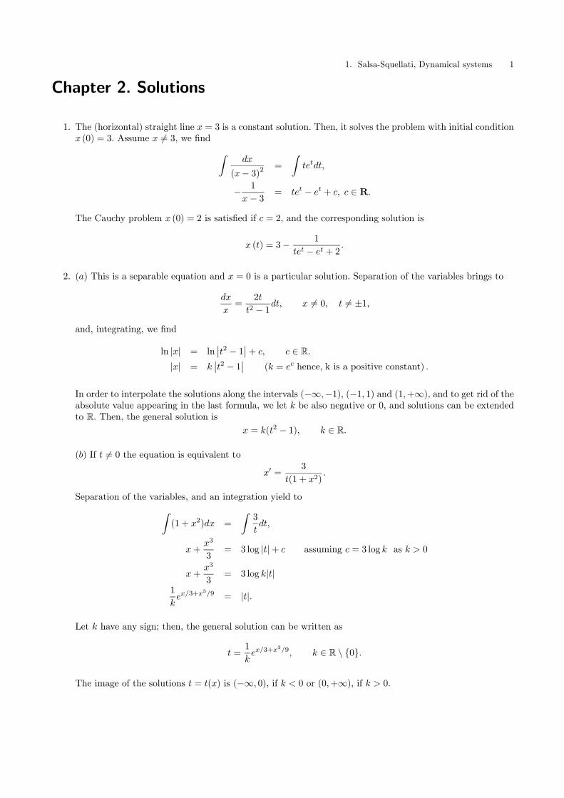
7. Consider s ≤ b, we apply to f in the interval [a, s], the fundamental theorem of integral calculus:

f(s)− f(a) =

Z s

a

f 0(u) du.

We deduce:

|f(s)− f(a)| =

¯Z s

a

f 0(u) du

¯≤

Z s

a

|f 0(u)| du

≤ k(s− a)

≤ k|s|+ k|a|


0 20 2

Figura 1.1.

hence,|f(s)| ≤ |f(a)|+ k|s|+ k|a|.

Consider now any (t, x0) ∈ S. We apply the previous formula in the x direction. We have:

|f(t, x)| ≤ |f(t, x0)|+ k|x|+ k|x0| ≤ c+ k|x|

since f(t, a) is a continuous function over the compact [a, b], and then it is bounded.

8. We have x0 (t) = a [M − x (t)], whose solution is x (t) =M (1− e−at).

9. As shown in the phase diagram Figure 1.1, equilibria are x = 0 (semistable) and x = 2 (unstable).

10. Let ϕ (t) be a T -periodic solution of the equation x0 = f (x) , then

ϕ (T ) = ϕ (0) .

Applying the Rolle theorem, there exists a point t0 where

ϕ0 (t0) = 0.

If x0 = ϕ (t0) , then substituting into the equation, we obtain

f (x0) = 0

and then the solution of the problem ½x0 = f (x)x (t0) = x0

is the constant ψ (t) ≡ x0. The local existence and uniqueness theorem requires that ϕ and ψ coincide, thusϕ is constant.

11. (a) The function f (x) = 3√x is derivable on R\{0}. The local existence and uniqueness theorem hypothesis

are then satisfied for k 6= 0.(b) If k = 0, x = 0 is a solution. We search for the general solution of the equation. Consider x 6= 0,separation of the variables gives

dx3√x

= dt

3

2

3√x2 = t+ c, c ∈ R

x = ±

sµ2

3t+ c

¶3


The functions

x =

⎧⎪⎨⎪⎩0 t ≤ 0sµ2

3t

¶3t > 0

and

x =

⎧⎪⎨⎪⎩0 t ≤ 0

−

sµ2

3t

¶3t > 0

both solve the problem with the initial condition x (0) = 0 but they are locally different functions. We arguethat the (local) uniqueness of the solution does not hold, not even locally.

12. We denotef(t, x) =

2

tx+ 2t

√x,

and deducefx(t, x) =

2

t+

t√x;

then, f is continuous for (t, x) ∈ (0,+∞)× [0,+∞), and fx is continuous for (t, x) ∈ (0,+∞)× (0,+∞).The continuity of f ensures the existence of at least one solution. For x = 0, the sufficient hypothesisguaranteeing uniqueness does not hold.

It is immediate to see that x = 0 is a solution. On the other hand, integration of the Bernoulli equation,when you set z =

√x, gives

z0 =1

tz + t,

z= t(t+ c), c ∈ R,

and we deduce the general solutionx = t2(t+ c)2.

These solutions are defined for t(t+ c) ≥ 0.In particular, for c = −1 we find a solution whose domain is t ≥ 1 (and it can be connected with x = 0 fort < 1).

This problem has, then, multiple local solutions.

The particular solution x = 0 is also known as boundary solution, since it coincide with the boundary ofthe set where the existence and uniqueness theorem holds.

13. The hypothesis (a) and (b) bring to the equation

d

dtI(t) = αIS − βI

recalling that S(t) + I(t) = N , we deduce that the illness evolution model is described by the differentialequation

d

dtI(t) = (αN − β)I(t)− αI(t)2. (1.2)

Denote by N0 (0 < N0 < N) the number of individuals infected at time t = 0. Integrating the separableequation (1.2), for αN − β = 0, we have:

I(t) =N0

αt+ 1

and thenlim

t→+∞I(t) = 0;


meaning that the whole population is due to become healthy.

As αN − β 6= 0, the equation (1.2) can be integrated using the Bernoulli technique or, again, consideringit as a separable equation. Its solution is

I(t) =(αN − β)N0

(αN − αN0 − β)e(β−αN)t + αN0

and we deduce that

limt→+∞

I(t) =

⎧⎪⎨⎪⎩0 0 < N <

β

ααN − β

αN >

β

α.

Then, two kind of longtime behavior might be expected: if 0 < N ≤ β

α, the infection will vanish; instead,

if N >β

αthe number of infected people will reach the endemic level

αN − β

α.

14. We assume that F ∈ C∞(R3). The differential equation of the family is found eliminating c between theequations ½

2y + 2x2 − 4cx+ c2 = 02y0 + 4x− 4c = 0,

(the second equation is obtained by differentiation of the first one). Solve the latter equation with respectto c, and substitute into the former to obtain

2y + 2x2 − (2y0 + 4x)x+µy0 + 2x

2

¶2= 0

that isy02 − 4xy0 − 4x2 + 8y = 0.

15. Equilibria solve the equation f (x) = x3 − 2x2 +mx =¡x2 − 2x+m

¢x = 0. According to the value of m,

we have:

X if m > 1, x = 0;

X if m = 1, x = 0 and x = 1;

X if 0 < m < 1, x = 0 and x = 1±√1−m (both of them are positive).

Since f 0 (x) = 3x2 − 4x+m, we obtainf 0 (0) = m > 0.

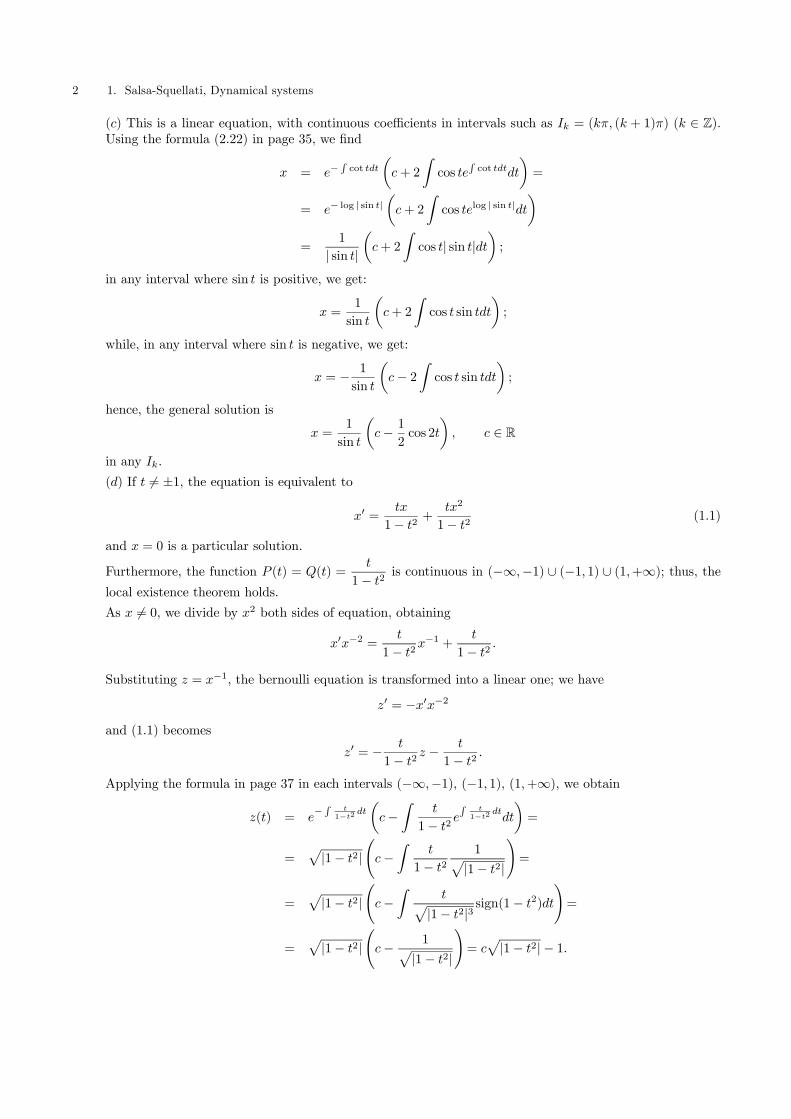
Then, for every m > 0 the point x = 0 is an unstable equilibrium. The phase diagram representing thecases m = 1 and m > 1 is in Figure 1.2.

If m = 1, the point x = 1 is a semistable equilibrium; if 0 < m < 1 the two equilibria x = 1−√1−m and

x = 1 +√1−m are respectively asymptotically stable and unstable equilibrium.


1. The general solution of the first problem is

sn = c

µ−13

¶n, c ∈ R;

as a consequence, for every c ∈ R we have sn → 0.


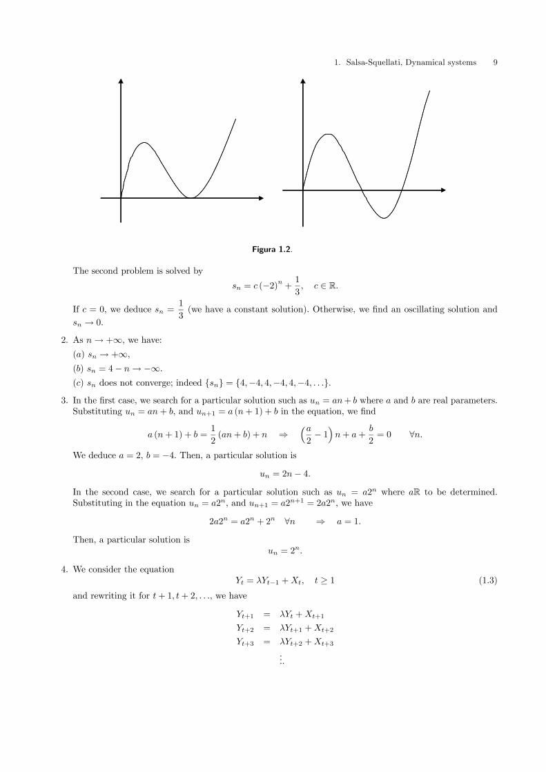
Figura 1.2.

The second problem is solved by

sn = c (−2)n + 13, c ∈ R.

If c = 0, we deduce sn =1

3(we have a constant solution). Otherwise, we find an oscillating solution and

sn → 0.

2. As n→ +∞, we have:(a) sn → +∞,(b) sn = 4− n→ −∞.

(c) sn does not converge; indeed {sn} = {4,−4, 4,−4, 4,−4, . . .}.

3. In the first case, we search for a particular solution such as un = an+ b where a and b are real parameters.Substituting un = an+ b, and un+1 = a (n+ 1) + b in the equation, we find

a (n+ 1) + b =1

2(an+ b) + n ⇒

³a2− 1´n+ a+

b

2= 0 ∀n.

We deduce a = 2, b = −4. Then, a particular solution is

un = 2n− 4.

In the second case, we search for a particular solution such as un = a2n where aR to be determined.Substituting in the equation un = a2n, and un+1 = a2n+1 = 2a2n, we have

2a2n = a2n + 2n ∀n ⇒ a = 1.

Then, a particular solution isun = 2

n.

4. We consider the equationYt = λYt−1 +Xt, t ≥ 1 (1.3)

and rewriting it for t+ 1, t+ 2, . . ., we have

Yt+1 = λYt +Xt+1

Yt+2 = λYt+1 +Xt+2

Yt+3 = λYt+2 +Xt+3

....


Divide the first by λ, the second by λ2, and so on, to deduce

1

λYt+1 = Yt +

1

λXt+1

1

λ2Yt+2 =

1

λYt+1 +

1

λ2Xt+2

1

λ2Yt+3 =

1

λ2Yt+2 +

1

λ2Xt+3

... .

Add side by side; cancelation of the terms like1

λYt+1,

1

λ2Yt+3, . . . yields to

0 = Yt ++∞Xi=1

µ1

λ

¶iXt+i.

Since {Xt} is bounded and λ > 1, we point out that the series+∞Xi=1

µ1

λ

¶iXt+i is convergent. The last

formula gives that

Yt = −+∞Xi=1

µ1

λ

¶iXt+i

is a particular solution of the equation (1.3). Thus, the general solution of the equation is

Yt = cλt −+∞Xi=1

µ1

λ

¶iXt+i, c ∈ R;

they diverge all, but the particular solution.

5. We consider the functiong (x) = f (x)− x;

g is continuous in [a, b]. Furthermore,

g (a) = f (a)− a ≥ 0, g (b) = f (b)− b ≤ 0.

If f (a) = a, then a is a fixed point for f ; if f (b) = b, then b is a fixed point for f . If neither f (a) = a, norf (b) = b, we have

g (a) > 0 and g (b) < 0,

and hence the continuous function g has at least one zero in (a, b), i.e. there exists x∗ ∈ (a, b) and

g (x∗) = f (x∗)− x∗ = 0.

As a consequence x∗ solves the equation f (x) = x, namely, it is a fixed point for f.

6. On account of the continuity of f , we have

limn→+∞

f (xn) = f

µlim

n→+∞xn

¶= f (l)

Using the recurrence equation, the uniqueness of the limit and the fact that xn+1 → l, we deduce

xn+1 = f (xn)↓ ↓l = f (l) ,

thus, l is a fixed point for f


7. First, we consider x1 > x0. We want to prove that for every n > 1,

p (n) : xn > xn−1.

We shall use mathematical induction on the statement p(n). First, we prove that the statement is true forn = 1; then we prove that if the statement is true for n, then it is true for n+ 1.

By hypothesis, p (n) is true for n = 1. We prove that p (n) ⇒ p (n+ 1) . Assuming p (n) is true, since f isincreasing, we deduce

f (xn) > f (xn−1) ,

that isxn+1 > xn

then, p (n+ 1) is true. Induction concludes that p (n) is true for every n ≥ 1; that is, xn is increasing.We can repeat the reasoning for x1 < x0, deducing that xn is decreasing. In any case, xn is monotonic,hence, it is regular.

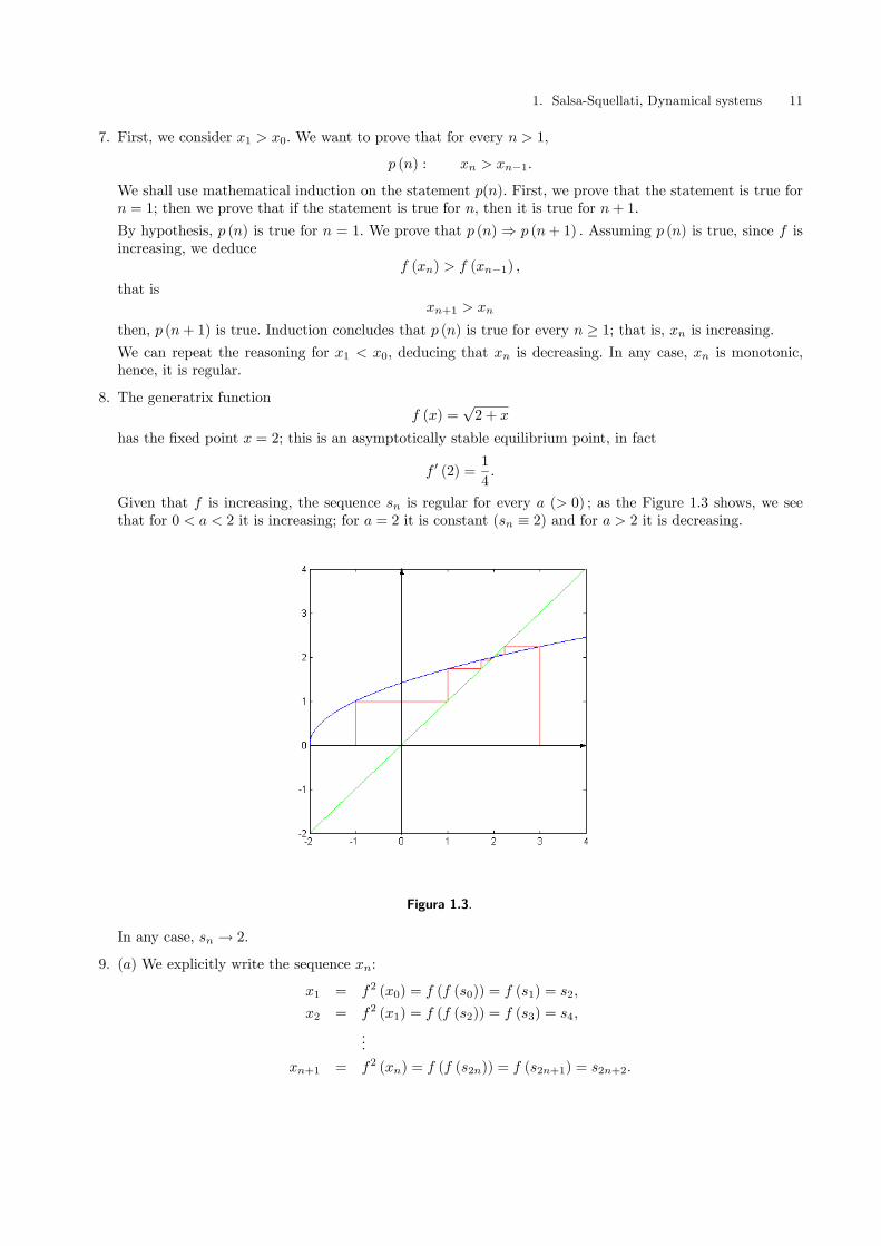
8. The generatrix functionf (x) =

√2 + x

has the fixed point x = 2; this is an asymptotically stable equilibrium point, in fact

f 0 (2) =1

4.

Given that f is increasing, the sequence sn is regular for every a (> 0) ; as the Figure 1.3 shows, we seethat for 0 < a < 2 it is increasing; for a = 2 it is constant (sn ≡ 2) and for a > 2 it is decreasing.

Figura 1.3.

In any case, sn → 2.

9. (a) We explicitly write the sequence xn:

x1 = f2 (x0) = f (f (s0)) = f (s1) = s2,

x2 = f2 (x1) = f (f (s2)) = f (s3) = s4,

...

xn+1 = f2 (xn) = f (f (s2n)) = f (s2n+1) = s2n+2.


The proof for yn is analogous.

(b) Since f2 is increasing1, xn and yn are monotonic. If xn = s2n is increasing, namely if s2n < s2n+2, wededuce that

s2n+1 = f (s2n) > f (s2n+2) = s2n+3

since f is decreasing; thus, yn = s2n+1 is decreasing. The other cases are analogous.

(c) If xn = s2n → x∗ (x∗ is a fixed point for f2), then the continuity of f implies that yn = s2n+1 =f (s2n) → f (x∗). If yn = s2n+1 → y∗ (y∗ is a fixed point for f2), then, the continuity of f implies thatxn = s2n = f (s2n−1) → f (y∗). Thus, the uniqueness of the limit gives x∗ = f (y∗) and y∗ = (x∗) . Inparticular, if f2 has the same fixed points2 of f , we deduce x∗ = y∗.

(d) If x∗ = y∗ = l then s2n → l, s2n+1 → l and hence sn → l. Viceversa, if sn → l then we have alsoxn = s2n → l and yn = s2n+1 → l, thus, x∗ = y∗ = l.

10. Introducing xn+1 = f (xn), the generatrix function is f (x) =1

2

µx+

A

x

¶. The fixed points of f solve

x =1

2

µx+

A

x

¶;

they are x = ±√A. Given that f 0 (x) =

1

2

µ1− A

x2

¶and f 0

³±√A´= 0, both of them are locally

asymptotically stable equilibria.

Consider, for instance, the recurrence sequence defined by the equation⎧⎨⎩ xn+1 =1

2

µxn +

7

xn

¶x0 = 4.

(1.4)

As the phase diagram in Figure 1.4 shows, the solution of the problem (1.4) converges to√7. We find

0 1 2 3 4 5 60

1

2

3

4

5

6

Figura 1.4. Phase diagram for the solution of the problem (1.4)

1We recall that, if f is decreasing, then f ◦ f is increasing.2We remind that any fixed point for f is a fixed point for every iterate fk. The converse is not true.


x1 =1

2

µ4 +

7

4

¶=23

8= 2.875, x2 =

1

2

µ2.875 +

7

2.875

¶' 2. 6549

x3 =1

2

µ2. 6549 +

7

2. 6549

¶' 2. 6458 x4 =

1

2

µ2. 6458 +

7

2. 6458

¶' 2. 6458

After three iteracions, we have three exact decimal digits.

11. The generatrix function is

f (x) =2

1 + x.

In order to determine the fixed points of f, we solve the equation

x =2

1 + x,

that is x2 + x− 2 = 0. The fixed points are x = −2 and x = 1. Since f 0 (x) = − 2

(1 + x)2 , we deduce that

f 0 (−2) = −2 and f 0 (1) = −12.

Given that|f 0 (−2)| > 1 and |f 0 (1)| < 1,

the point x = −2 is an unstable equilibrium, and the point x = 1 is an asymptotically stable equilibrium.For a = 1, the solution is constant. For every a > 0 (a 6= 1), the corresponding solution sn converges to1 with oscillating behavior. We verify this fact considering, for instance, a ∈ (0, 1) . Using the results ofexercise 9, the sequences s2n and s2n+1 are monotone (and regular). In particular, if s0 ∈ (0, 1) , s2n isincreasing and s2n+1 is decreasing. Furthermore, we find that

f2 (x) = f (f (x)) =2

1 + 2/ (1 + x)=2 + 2x

3 + x

has the same fixed points of f, since the equation

2 + 2x

3 + x= x

is equivalent to x2 + x − 2 = 0. Thus, s2n → 1 and s2n+1 → 1 and, as a consequence sn → 1. The casea > 1 can be proved using the same argument.

The behavior of sn is sketched in Figure 1.5.

12. The equilibrium equation is

pt+1 = pt + σ (a− bpt + c− dpt) = [1− σ (b+ d)] pt + σ (a+ c)

And it is solved bypt = [1− σ (b+ d)]

t(p0 − p∗) + p∗,

Where p∗ =a+ c

b+ d. Then pt converges to p∗, if and only if |1− σ (b+ d)| < 1, namely if σ <

2

b+ d.

13. (a) The generatrix function isf (x) = xe1−x

3/3.

We draw its graph in the first quardrant, where the function is non negative. We deduce that

f (0) = 0 and limx→+∞

f (x) = 0+.


0 1 2 3 4 5 60

0 . 5

1

1 . 5

2

2 . 5

3

Figura 1.5.

0 0.5 1 1.5 2 2.5 30

0.5

1

1.5

2

2.5

3

Figura 1.6. Graph of f (x) = xe1−x3/3

Since

f 0 (x) =¡1− x3

¢e1−x

3/3,

f 0 (x) = 0 as x = 1;

henceforth, x = 1 is a maximum. (b) The fixed points of f solve the equation

xe1−x3/3 = x.

They arex = 0 and x =

3√3.

Given thatf 0 (0) = e > 1 and f 0

³3√3´= −2 < −1

both of them are unstable equilibria.


14. (a) The equilibrium points solve the equation

x = f (x) =αx

1 + βx;

they are x = 0 and, when α 6= 1, x = α− 1β

. Since

f 0 (x) =α

(1 + βx)2 ,

we have

f 0 (0) = α, f 0µα− 1β

¶=1

α.

Therefore, if 0 < α < 1, x = 0 is a stable equilibrium, and x =α− 1β

(< 0) is an unstable equilibrium; if

α > 1, x = 0 is an unstable equilibrium and x =α− 1β

is a stable equilibrium.

In the case α = 1, the only fixed point is x = 0 and since f 0 (0) = 1, the linearization criterion cannot beapplied. A deeper analysis would be necessary to determine the stability nature of this point.

The dynamics in a neighborhood of the fixed points is monotonic since f 0 is positive for every x ≥ 0, andthus f is increasing.

(b) When α = β = 1, the phase diagram is represented in the Figure 1.7, and we deduce that, for everyx0 > 0 xn → 0 (indeed, this is the behavior for every β).

-0.5 0 0.5 1 1.5 2 2.5 3 3.5 4 4.5-0 .5

0

0.5

1

1.5

2

2.5

Figura 1.7.

(c) Consider (xn+1 =

xn1 + xn

x0 > 0.

We have

x1 =x0

1 + x0, x2 =

x01 + x0

1 +x0

1 + x0

=x0

1 + 2x0, x3 =

x01 + 2x0

1 +x0

1 + 2x0

=x0

1 + 3x0, . . . ,


and we deducexn =

x01 + nx0

,

converging to zero for every x0 > 0.


1. The linear differential equations are:

(a) x00 (t) = 0;

(b) x00 (t) + x0 (t) = 0,

(b) x00 (t) + 5x0 (t) + 6x (t) = 0.

2. (a) The characteristic equation of the associated homogeneous equation is

λ2 − 1 = 0

whose solutions are λ12 = ±1. A candidate particular solution is u (t) = a sin t, and we deduce a = −12.

The general solution is

x (t) = c1et + c2e

−t − 12sin t c1, c2 ∈ R.

(b) The characteristic equation of the associated homogeneous equation is

λ2 + 1 = 0

whose solutions are λ12 = ±i. A particular solution of the complete equation is u (t) = 2t −3. The generalsolution is

x (t) = c1 cos t+ c2 sin t+ 2t− 3, c1, c2 ∈ R.

(c) The characteristic equation of the associated homogeneous equation is

λ2 − 2λ+ 2 = 0

whose solutions are λ12 = 1 ± i. As a particular solution of the complete equation we use u (t) = at + b,

deriving and substituting into the differential equation we deduce a = 2, b =7

2. The general solution is

x (t) = et (c1 sin t+ c2 cos t) + 2t+7

2, c1, c2 ∈ R.

3. (a) The general solution isx (t) = c1 cos t+ c2 sin t, c1, c2 ∈ R.

The constants c1 and c2 are found solving the system⎧⎨⎩ x³π2

´= c2 = 0

x0³π2

´= −c1 =

π

2.

The solution of the Cauchy problem isx (t) = −π

2cos t.

(b) The general solution of the differential equation is

x (t) = c1e−2t + c2e

2t − 13et.


In order to solve the Cauchy problem, we compute x0

x0 (t) = −2c1e−2t + 2c2e2t −1

3et.

On account of the initial conditions, we deduce the system⎧⎪⎨⎪⎩c1 + c2 −

1

3= 0

−2c1 + 2c2 −1

3= 0;

hence, ⎧⎪⎨⎪⎩c1 =

1

12

c2 =1

4.

The solution of the Cauchy problem is

x (t) =1

12e−2t +

1

4e2t − 1

3et.

4. The solution of the characteristic equation is 1 (with multiplicity 2).

(a) Since 0 is not a solution of the characteristic equation, as a candidate particular solution we choose

u = At3 +Bt2 + Ct+D.

Substituting into the equation, we find A, B, C, D, and have

u = t3 − 6t− 12.

(b) Since 2 is not a solution of the characteristic equation, while 1 is (with double multiplicity), as acandidate particular solution we choose

u = At2et +Be2t.

Substituting into the equation, we obtain

u =1

2t2et + e2t.

(c) Since 1± i are not solutions of the characteristic equation, as a candidate particular solution we choose

u = et(A sin t+B cos t).

Substituting into the equation, we haveu = −et sin t.

5. (a) The roots of the characteristic equation are 1 and −12±√3

2i. The general solution is

y = c1et + e−t/2

Ãc2 cos

Ã√3

2t

!+ c3 sin

Ã√3

2t

!!,

where c1, c2, c3 are arbitrary real constants.

The positive root of the characteristic equation implies that the zero solution is an unstable equilibrium.

(b) The characteristic equation’s root are 0 and ±√2i, both with multiplicity 2.



y = c1 + c2t+ (c3 + c4t) cos³√2t´+ (c5 + c6t) sin

³√2t´,

where ci, i = 1, . . . , 6 are arbitrary constants.

The characteristic equation has roots with zero real part; given that they are not simple, the zero solutionis an unstable equilibrium.

6. (a) The roots of the characteristic equation are ±i, with multiplicity 2. Since 0 is not a solution of thecharacteristic equation, as a particular solution, we choose

u = At2 +Bt+ C.

Substituting into the equation, we are yield to find A = 1, B = 0, C = −4.The general solution is then

y = (c1 + c2t) sin t+ (c3 + c4t) cos t+ t2 − 4,

where ci ∈ R, i = 1, . . . , 4.(b) The roots of the characteristic equation are 1, with multiplicity 2 and −2, simple.Since 1 is a double root of the characteristic equation, as a particular solution we choose

u = et(At2 +Bt+ C).

We find A =1

36, B = − 1

27, C =

1

27.


y = c1e−2t + et

µc2 + c3t+

t2

27− t3

27+

t4

36

¶,

where c1, c2, c3 ∈ R.

(c) The roots of the characteristic equation are −2 and −23.

Since −1 and ±i don’t solve the characteristic equation, as a particular solution we choose

u = Ae−t +B sin t+ C cos t.

We are yield to find A = −1, B =1

65, C = − 8

65.


y = c1e−2t + c2e

−2t/3 − e−t +1

65sin t− 8

65cos t,

with c1, c2 ∈ R.

7. The characteristic equation isλ3 − 2λ2 + λ = 0,

whose solutions are 0 and 1 (double root), corresponding to the following solutions of the differentialequation: 1, et, and tet.

Given that 1 is a double root of the characteristic equation, as a particular solution we choose

u(t) = At2et.

We obtain that

u0(t) = A(t2 + 2t)et, u00(t) = A(t2 + 4t+ 2)et, u000(t) = A(t2 + 6t+ 6)et


and, substituting into the differential equation, we obtain:

A(t2 + 6t+ 6)et − 2A(t2 + 4t+ 2)et +A(t2 + 2t)et = et,

and hence

A =1

2.

Thus, the general solution is

y = c1 + c2et + c3te

t +1

2t2et. (1.5)

The constants c1, c2, c3 are to be determined in order to satisfy the initial conditions.

Deriving (1.5), we obtain:

y0 = c2et + c3 (t+ 1) e

t +1

2

¡t2 + 2t

¢et

y00 = c2et + c3 (t+ 2) e

t +1

2

¡t2 + 4t+ 2

¢et.

On account of the initial conditions, we are yield to the system⎧⎨⎩ c1 + c2 = 0c2 + c3 = 0c2 + 2c3 + 1 = 0,

solved byc1 = −1, c2 = 1, c3 = −1.

The solution of the Cauchy problem is

y = −1 +µ1− t+

1

2t2¶et.

8. The zero solution is stable, thanks to the stability criterion for third order equations (we have positivecoefficients and 6 · 9 > 1).

9. The characteristic equation isλ2 + 2δλ+ ω2 = 0.

We analyze three cases.

If δ > ω the characteristic equation has two (negative) distinct real roots

λ1 = −δ −pδ2 − ω2 and λ2 = −δ +

pδ2 − ω2

and the general solution isy (t) = C1e

λ1t + C2eλ2t, C1, C2 ∈ R.

If δ = ω the characteristic equation has one double root λ12 = −δ and the general solution is

y (t) = (C1 + C2t) e−δt, C1, C2 ∈ R.

If δ < ω the characteristic equation has complex roots λ12 = −δ ± ipω2 − δ2 and the general solution is

y (t) = e−δt (C1 sin νt+ C2 cos νt) , C1, C2 ∈ R,

denoting ν =pω2 − δ2. Anyhow, we have that limt→+∞ y (t) = 0.



1. The characteristic equation isλ2 − 5λ+ 6 = 0

whose solutions are λ1 = 2 and λ2 = 3. Therefore, the general solution is

xn = C12n + C23

n, C1, C2 ∈ R.

In order to satisfy the Cauchy problem x0 = 0 and x1 = 1, we solve the system½C1 + C2 = 02C1 + 3C2 = 1,

and deduceC1 = −1, C2 = 1.

Then, the particular solution isxn = −2n + 3n.

2. (a) The characteristic equation is2λ2 − 3λ+ 1 = 0,

thus, λ1 =1

2, and λ2 = 1. The general solution is

xn = C1

µ1

2

¶n+ C2, C1, C2 ∈ R.

The zero solution is neutrally stable.

(b) The characteristic equation isλ2 + 1 = 0

whose roots are ±i. The general solution is

xn = C1 sinnπ

2+ C2 cosn

π

2,

where C1 and C2 are real, arbitrary constants. The zero solution is neutrally stable.

(c) The characteristic equation isλ2 − 4λ+ 4 = 0,

then, 2 is a 2-multiplicity root. A particular (constant) solution is un = 1. Therefore, the general solutionis

xn = 2n (C1 + C2n) + 1, C1, C2 ∈ R.

The constant solution is unstable.

3. (a) The characteristic equation isλ2 − 3λ+ 2 = 0

whose roots are λ = 1 and λ = 2. We search for a particular solution of the complete equation such asxn = A3n. Substituting into the equation, we find A = 1/2. Then, the general solution is

xn = c1 + c22n +

1

23n, c1, c2 ∈ R.

(b) The characteristic equation isλ3 − λ2 + λ− 1 = 0.


Its roots are λ1 = 1, and λ23 = ±i. We seek for a particular solution such as un = An; we are yield to find

A (n+ 3)−A (n+ 2) +A (n+ 1)−An = −1

and deduce A = −12. The general solution of the equation is

xn = c1 + c2 cosnπ

2+ c3 sinn

π

2, c1, c2, c3 ∈ R.

4. The characteristic equation isλ3 + 1 = 0

with roots λ1 = −1, and λ2,3 =1

2±√3

2i = cos

π

3± i sin

π

3. The general solution of the equation is

xt = c1 (−1)t + c2 sinπt

3+ c3 cos

πt

3c1, c2, c3 ∈ R.

Considering the initial value problem x0 = 1, x1 = 0, x2 = 2, we obtain the system⎧⎪⎪⎪⎨⎪⎪⎪⎩c1 + c3 = 1

−c1 +√3

2c2 +

1

2c3 = 0

c1 +

√3

2c2 −

1

2c3 = 2;

solved by c1 = 1, c2 =2√3

3, and c3 = 0. The solution of the Cauchy problem is

xt = (−1)t +2√3

3sin

πt

3.

We point out that

xt+6 = (−1)t+6 +2√3

3sin

π (t+ 6)

3= xt

then, xt is 6-periodic.

5. We tell two cases: λ1, λ2 ∈ R and λ1, λ2 complex conjugate.

Case 1. Considering real roots, from |λ1| < 1 and |λ2| < 1, we deduce |λ1λ2| < 1.If λ1 and λ2 have the same sign λ1λ2 = |λ1λ2|, hence

λ1λ2 < 1. (1.6)

On the other hand, (1.6) holds if the roots λ1 and λ2have opposite sign or one of them is zero, too.

From −1 < λ1 < 1 and −1 < λ2 < 1, we deduce

(1− λ1) (1− λ2) > 0, (1 + λ1) (1 + λ2) > 0 (1.7)

namely1 + λ1λ2 > λ1 + λ2, 1 + λ1λ2 > −λ1 − λ2

and thus|λ1 + λ2| < 1 + λ1λ2. (1.8)

Viceversa, if (1.8) holds, then (1.7) and (1.6) imply

|λ1| < 1 and |λ2| < 1.


Actually, (1.7) hold if both roots are less than −1 or if both roots are grater than 1, too; but in thesesituations their product would be grater than 1.

Case 2. If the roots are complex and conjugate, i.e. λ12 = α ± iβ, we have |λ1| = |λ2| =pα2 + β2,

λ1λ2 = α2 + β2 and we immediately deduce that

|λ1| < 1 and |λ2| < 1 ⇐⇒ λ1λ2 < 1.

The condition (1.8) is true for every pair of complex and conjugate numbers; in fact λ1+λ2 = 2α and (1.8)becomes

|2α| < 1 + α2 + β2

that is(1− |α|)2 + β2 > 0.

6. (a) The zero solution is asymptotically stable if and only if the roots of the characteristic equation areinside the circumference of radius 1 (i.e. their modulus is less than 1). The characteristic equation is

λ2 − λ− a = 0

its roots have a less than 1 modulus if

−a < 1, 1 < 1− a,

therefore, the zero solution is asymptotically stable if and only if

−1 < a < 0.

(b) The characteristic equation is

λ2 − λ− 18= 0

with roots

λ12 =1

2±r3

8.


xt = c1

Ã1

2+

r3

8

!t

+ c2

Ã1

2−r3

8

!t

, c1, c2 ∈ R.

In order to find the solution satisfying the initial conditions x0 = 0, and x1 = 10, we determine c1 and c2solving the system ⎧⎪⎨⎪⎩

c1 + c2 = 0

c1

Ã1

2+

r3

8

!+ c2

Ã1

2−r3

8

!= 10.

We are led to ⎧⎪⎪⎨⎪⎪⎩c1 = 10

r2

3

c2 = −10r2

3.

The solution is

xt = 10

r2

3

⎡⎣Ã12+

r3

8

!t

−Ã1

2−r3

8

!t⎤⎦ .


7. The model is described by the second order equation

Yt − (1− s− v)Yt−1 + vYt−2 = A0 (1 + g)t . (1.9)

We search for a particular solution such as Y t = kmt where m = 1 + g. Substituting into (1.9), we find

kmt − (1− s− v) kmt−1 + vkmt−2 = A0mt

mt−2 ¡km2 − km (1− s− v) + kv −A0m2¢= 0

thus

k =A0m

2

m2 − (1− s− v)m+ v.

The particular solution is

Y t =A0m

2+t

m2 − (1− s− v)m+ v.

If the solutions of the homogeneous equation tend to 0 as t→ +∞, namely if the roots of the characteristicequation λ2 − (1− s− v)λ+ v = 0 are, in modulus, less than 1 (i.e. when v < 1), then all the solutions ofthe complete equation tend to Y t.

On the other hand, if the solutions of the homogeneous equation don’t tend to 0, the solutions of thecomplete equation will diverge or oscillate, according to the sign of the discriminant of the characteristicequation.


1. The eigenvalues of the coefficients’ matrix are λ1 = −4, λ2 = 1, corresponding, for instance, to the eigen-vectors

u1 =

µ−11

¶and u2 =

µ32

¶.

The general solution is µxy

¶= c1

µ−11

¶e−4t + c2

µ32

¶et

where c1 and c2 are arbitrary constants. The zero solution is not stable.

2. The eigenvalues of the coefficients’ matrix are λ1 = 0, λ2 = −2 corresponding, for instance, to the eigen-vectors

u1 =

µ34

¶and u2 =

µ12

¶.

The general solution is µxy

¶= c1

µ34

¶+ c2

µ12

¶e−2t

where c1 and c2 are arbitrary constants. The initial condition gives½0 = 3c1 + c22 = 4c1 + 2c2,

=⇒½

c1 = −1c2 = 3

and, therefore, the solution if the Cauchy problem isµxy

¶= −

µ34

¶+ 3

µ12

¶e−2t.


3. (a) From the first equation we deduce y = −x0 + x, derivation gives y0 = −x00 + x0. Substitution into thesecond equation gives

−x00 + x0 = x− x0 + x,

namelyx00 − 2x0 + 2x = 0.

The characteristic equationλ2 − 2λ+ 2 = 0

has complex roots λ = 1± i. Thus,x = et (c1 cos t+ c2 sin t)

where c1 and c2 are real constants. Now, we compute

x0 = et (c1 cos t+ c2 sin t) + et (−c1 sin t+ c2 cos t)

andy = −x0 + x = et (c1 sin t− c2 cos t) .

The general solution of the system is ½x = et (c1 cos t+ c2 sin t)y = et (c1 sin t− c2 cos t) .

The solution of the system can also be written asµxy

¶= c1

µcos tsin t

¶et + c2

µsin t− cos t

¶et.

(b) We solve the first equation, obtainingx = c1e

2t.

A substitution into the second equation gives

y0 = 2y + c1e2t

whose general solution isy = c2e

2t + c1te2t.

The system’s general solution is ½x = c1e

2t

y = c2e2t + c1te

2t.

4. (a) The coefficients’ matrix is

A =

µ−1 −21 −1

¶we find

tr A = −2 < 0 and detA = 3 > 0

therefore, the zero solution of the system is asymptotically stable.

(b) The coefficients’ matrix has positive trace (thus, at least one eigenvalue is positive). We argue that thezero solution is unstable.


5. The coefficients’ matrix has eigenvalues λ1 = −1, λ2 = 1, λ3 = 3, corresponding, for instance, to theeigenvectors

u1 =

⎛⎝ 121

⎞⎠ , u2 =

⎛⎝ 101

⎞⎠ and u3 =

⎛⎝ 1−12

⎞⎠ .

The general solution is ⎛⎝ xyz

⎞⎠ = c1

⎛⎝ 121

⎞⎠ e−t + c2

⎛⎝ 101

⎞⎠ et + c3

⎛⎝ 1−12

⎞⎠ e3t

where c1, c2 and c3 are arbitrary constants. The initial condition gives⎧⎨⎩ 3 = c1 + c2 + c31 = 2c1 − c3,4 = c1 + c2 + 2c3

=⇒

⎧⎨⎩ c1 = 1c2 = 1c3 = 1

then, the solution of the Cauchy problem is⎛⎝ xyz

⎞⎠ =

⎛⎝ 121

⎞⎠ e−t +

⎛⎝ 101

⎞⎠ et +

⎛⎝ 1−12

⎞⎠ e3t.

6. The coefficients’ matrix is triangular; then, the elimination method may be suggested. We find⎧⎨⎩ x = c1et

y = c1et + c2e

2t

z = −c1et + c2te2t + c3e

2t.

The initial condition gives ⎧⎨⎩ 1 = c10 = c1 + c2,1 = −c1 + c3

=⇒

⎧⎨⎩ c1 = 1c2 = −1c3 = 2

and, then, the solution of the Cauchy problem is⎧⎨⎩ x = et

y = et − e2t

z = −et − te2t + 2e2t.

7. Both systems have an unstable zero solution.

8. (a) The coefficients’ matrix is

A =

µ−1 12a a

¶.

The origin is asymptotically stable if and only if

detA > 0 and trA < 0;

that is, if and only if−3a > 0 and − 1 + a < 0,

hence, fora < 0.

(b) The coefficients’ matrix is

A =

µ−1 14 2

¶


whose eigenvalues areλ = −2 and λ = 3

corresponding, for instance, to the eigenvectorsµ−11

¶and

µ14

¶.

The general solution is µxu

¶= c1

µ−11

¶e−2t + c2

µ14

¶e3t, c1, c2 ∈ R.


1. (a) The eigenvalues of the coefficients’ matrix are1

2±√3

2i. They are complex and their real part is positive,

hence the origin is an unstable focus.

(b) The coefficients’ matrix has the 2-multiplicity (non regular) eigenvalue −2. Therefore, the origin is animproper node.

2. We have

d

dtE (x, y) = (2x+ y)x0 + (x+ 2y) y0 = (2x+ y) (−x− 2y) + (x+ 2y) (2x+ y) = 0.

The origin is a center.

3. (a) The origin is an isolated critic point. The eigenvalues of the coefficients’ matrix

A =

µ2 10 1

¶

are 2 and 1, and two corresponding eigenvectors are, for instance,µ10

¶and

µ−11

¶.

The steady state (0, 0) is an unstable proper node; the linear manifolds are y = 0 and y = −x.The straight line y = 0 is a particular solution. Since y = 0 if and only if y = 0, the trajectories have nopoints with horizontal slope. The vertical-slope isocline is y = −2x.The (homogeneous) equation of the trajectories is

y0 =dy

dx=

y

2x+ yfor 2x+ y 6= 0.

Introducing y = zx, we obtain:

z + xz0 =z

z + 2, xz0 = −z + z2

z + 2.

We deduce that z = 0 and z = −1 are particular solutions ( corresponding to y = 0 and y = −x).As y 6= 0, and y 6= −x, we have:

− z + 2

z + z2dz =

1

xdx, ln

|z + 1|z2

= ln |x|+ k, k ∈ R.


The equation of the family of trajectories is

y + x = cy2, c ∈ R,

with the straight line y = 0. Then, parabolae with horizontal axis, with vertex on the straight line y = −2xare union of trajectories.

(b) The coefficients’ matrix

A =

µ1 22 1

¶has the eigenvalues −1 and 3, corresponding, for instance, to the eigenvectors

µ−11

¶and

µ11

¶.

The straight line y = −x is a stable linear manifold, the straight line y = x is an unstable linear manifold.

The straight lines y = −2x and y = −12x are horizontal- and vertical-slope isoclines, respectively.

The (homogeneous) trajectories’ equation is

y0 =dy

dx=2x+ y

x+ 2yfor x+ 2y 6= 0.

Introducing y = zx, we obtain:

z + xz0 =2 + z

2z + 1, xz0 =

2−2z22z + 1

.

The straight lines z = 1 and z = −1 are particular solutions corresponding to y = x and y = −x.As y 6= x, and y 6= −x, we have:Z

2z + 1

1− z2dz =

2

xdx, −1

2ln¯(z + 1) (z − 1)3

¯= 2 ln |x|+ k, k ∈ R.

The orbits are represented by the equation

(y − x)3(y + x) = c, c ∈ R.

4. The equivalent system is ½x = yy = −x− ky

with the coefficient matrix

A =

µ0 1−1 −k

¶.

We havetr A = −k < 0, detA = 1 > 0, ∆ = k2 − 4.

We analyze the cases:∆ < 0, ∆ = 0, ∆ > 0.

If 0 < k < 2, the origin is a stable focus: the solutions tend to the steady state with oscillations.

If k = 2 the origin is an improper node.

If k > 2 the origin is a stable proper node. For every k ≥ 2, the solutions are definitively monotone.


5. (a) The steady states solve the system ½x+ y2 − 2 = 0x+ y = 0,

they are(1,−1), (−2, 2).

In order to determine their nature, we use the linearization criterion. The jacobian matrix associated tothe system is

A(x, y) =

µ1 2y1 1

¶.

Considering the point (1,−1), we have

detA = 3, tr A = 2, ∆ = (tr A)2 − 4 detA = −8.

Since A has complex eigenvalues (with positive real part), the point (1,−1) is an unstable focus for thelinearized system.

Considering the point (−2, 2), we find detA = −3. Since the eigenvalues of A are real and have oppositesign, the point (−2, 2) is a saddle for the linearized system.In view of the theorem 3.1, these results can be extended to the original system.

(b) The steady states solving the system ½−x+ x2y = 02− 2y = 0

are (0, 1) and (1, 1). The jacobian matrix associated to the system is

A(x, y) =

µ−1 + 2xy x2

0 −2

¶.

At (0, 1), we deducedetA = 2, tr A = −3, ∆ = 1;

therefore, (0, 1) is a (stable) proper node for the linearized system.

At (1, 1) we deducedetA = −2;

hence, (1, 1) is a saddle point for the linearized system. According to the theorem 3.1, these results can beextended to the original system.

6. The origin is the only steady state. We prove that it is a stable star. Indeed, on account of the theorem3.2, the coefficient matrix of the linearized system is

A =

µ−1 00 −1

¶and

f(x, y) = −x+ o¡ρ1+ε

¢,

given that|2x3y2| = |f(ρ, θ)| = 2ρ5| (cos θ)3 |(sin θ)2 ≤ 2ρ5.

Then, for every m, there exists a trajectory crossing the origin with slope m. More precisely, the axis x andy are union of trajectories (each straight line is made of three trajectories: two half straight line and thesteady state).


In order to find the vertical-slope isoclines, we solve x = 0, that is

x = 0 and 1− 2x2y2 = 0;

we deduce that the line 1−2x2y2 = 0 is a genuine vertical-slope isocline, while x = 0 is a trajectory, indeed.Instead, y is zero if and only if y = 0, that is, the straight line y = 0 is a horizontal-slope isocline and atrajectory of the system.

We find no genuine horizontal-slope isoclines. The figure 1.8 describes the phase diagram in the first quad-rant.

Figura 1.8.

7. (a) The equilibrium, solving the system ⎧⎪⎪⎨⎪⎪⎩−x2+

y

2= 0

− x

1 + x2+

y

2= 0

according to the conditions x > 0, y > 0,, is (1, 1) . The linearization criterion proves that it is a saddle. Infact, the jacobian matrix of the system, at (1, 1) isµ

−1/2 1/20 1/2

¶and it has real eigenvalues, with opposite sign.

(b) The vertical-slope isocline is y = x. The horizontal-slope isocline is y =2x

1 + x2.

(c) We find x > 0 as y > x; and we have y > 0 as y >2x

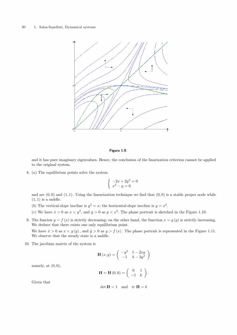
1 + x2. The phase portrait is in figure 1.9.

(d) No. In fact, the origin is a center for the linearized system, since the jacobian matrix at (0, 0) isµ−1/2 1/2−1 1/2

¶


Figura 1.9.

and it has pure imaginary eigenvalues. Hence, the conclusion of the linarization criterion cannot be appliedto the original system.

8. (a) The equilibrium points solve the system½−2x+ 2y2 = 0x2 − y = 0

and are (0, 0) and (1, 1) . Using the linearization technique we find that (0, 0) is a stable proper node while(1, 1) is a saddle.

(b) The vertical-slope isocline is y2 = x; the horizontal-slope isocline is y = x2.

(c) We have x > 0 as x < y2, and y > 0 as y < x2. The phase portrait is sketched in the Figure 1.10.

9. The funcion y = f (x) is strictly decreasing; on the other hand, the function x = g (y) is strictly increasing.We deduce that there exists one only equilibrium point.

We have x > 0 as x < g (y) , and y > 0 as y > f (x) . The phase portrait is represented in the Figure 1.11.We observe that the steady state is a saddle.

10. The jacobian matrix of the system is

H (x, y) =

µ−y2 1− 2xy−1 k − 3y2

¶namely, at (0, 0),

H = H (0, 0) =

µ0 1−1 k

¶.

Given thatdetH = 1 and tr H = k


Figura 1.10.

as k 6= 0 we use the linearization criterion.If k < 0, the zero solution is asymptotically stable for the linearized system and for the original system aswell. As k > 0, the zero solution is unstable both for the linearized and the original system.

As k = 0, we use the Liapunov technique. Consider the function

V (x, y) = x2 + y2,

this is (evidently) positive definite in R2. We have

V (x, y) = 2x¡y − xy2

¢+ 2y

¡−x− y3

¢= −2x2y2 − 2y4 ≤ 0

in R2. Thus, V is a Liapunov function for the system, and therefore the zero solution is asymptoticallystable.


1. (a) The eigenvalues of the coefficients’ matrix are λ1 = 1 and λ2 = 3; two corresponding eigenvectors are,

for instance,µ

1−1

¶and

µ11

¶, respectively. The general solution isµ

xtyt

¶= c1

µ1−1

¶+ c2

µ11

¶3t, c1, c2 ∈ R.

(b) In order to solve the initial value problem we have to solve the system½−2 = c1 + c22 = −c1 + 3c2.

We obtain c1 = −2, c2 = 0, then, the particular solution isµ

xtyt

¶=

µ−22

¶.


Figura 1.11.

2. The coefficients’ matrix is

A =

⎛⎝ 1 3 −20 2 40 1 2

⎞⎠and the associated characteristic equation is

det (A− λI) = (1− λ)h(2− λ)

2 − 4i= 0.

Its eigenvalues are λ0 = 0, λ1 = 1 and λ2 = 4, corresponding for instance, to the eigenvectors

v0 =

⎛⎝ 8−21

⎞⎠ , v1 =

⎛⎝ 100

⎞⎠ , v2 =

⎛⎝ 463

⎞⎠ ,

respectively, solutions of the systems⎧⎨⎩ x+ 3y − 2z = 02y + 4z = 0y + 2z = 0,

⎧⎨⎩ 3y − 2z = 0y + 4z = 0y + z = 0,

⎧⎨⎩ −3x+ 3y − 2z = 0−2y + 4z = 0y − 2z = 0.

The general solution of the system is, then,⎛⎝ xtytzt

⎞⎠ = c0ϕ0 + c1

⎛⎝ 100

⎞⎠+ c24t

⎛⎝ 463

⎞⎠ c0, c1, c2 ∈ R.

where ϕ0 =©v0,0,0,0, . . .

ª.

In order to determine the solution starting from x0 = (1, 1, 1)T, we search for c0, c1, c2 solving⎧⎨⎩ 1 = 8c0 + c1 + 4c2

1 = −2c0 + 6c21 = c0 + 3c2.

We are yield to c0 = 1/4, c1 = −2, c2 = 1/4.


3. (a) The coefficients’ matrix of the system is

A =

µ4 1−1 2

¶whose characteristic equation is

det (A− λI) = (4− λ) (2− λ) + 1 = λ2 − 6λ+ 9 = 0.

We find the eigenvalue λ = 3 with 2-multiplicity. The associated eigenspace solves½x+ y = 0−x− y = 0.

It has dimension 1, and is generated, for instance, by the eigenvectorµ

1−1

¶, associated to the eigenvalue

λ = 3. We search for a generalized eigenvector, solving the system½u+ v = 1−u− v = −1.

We find, for instance,µ10

¶.

The general solution of the system isµxtyt

¶= 3t

µc1

µ1−1

¶+ c2

µ1 + t1− t

¶¶, c1, c2 ∈ R.

The zero solution is unstable.

(b) The coefficients’ matrix of the system is

A =

µ1 1−3 1

¶with characteristic equation

det (A− λI) = (1− λ)2 + 3 = 0

with roots λ12 = 1±√3i = 2

³cos

π

3± i sin

π

3

´. An eigenvector associated to the eigenvalue 1+

√3i solves½

−√3iu+ v = 0

−3u−√3iv = 0.

For instance, we considerµ10

¶+

µ0√3

¶i. The general solution of the system is

µxtyt

¶= 2t

⎛⎝c1

⎛⎝ cosπt

3

−√3 sin

πt

3

⎞⎠+ c2

⎛⎝ sinπt

3√3 cos

πt

3

⎞⎠⎞⎠ , c1, c2 ∈ R.

The zero solution is unstable, since the modulus of the eigenvectors is grater than 1.

4. The coefficients’ matrix of the system is

A =

µ−0.3 0.70.6 −0.2

¶and we deduce

tr (A) = −0.5, det (A) = −0.36, |tr (A)| = 0.5 < 1 + det (A) = 0.64

therefore, using the stability criterion for 2-dimensional system, we deduce that the zero solution is asymp-totically stable.


5. (a) From the first equation, we obtain yt = −xt+1 + xt and then yt+1 = −xt+2 + xt+1; a substitution intothe second equation gives

xt+2 − 2xt+1 + 2xt = 0.The characteristic equation is

λ2 − 2λ+ 2 = 0

with roots 1± i =√2³cos

π

4± i sin

π

4

´; then,

xt = 2t/2

µc1 cos

πt

4+ c2 sin

πt

4

¶, c1, c2 ∈ R.

We deduce that

yt = −2(t+1)/2µc1 cos

π (t+ 1)

4+ c2 sin

π (t+ 1)

4

¶+ 2t/2

µc1 cos

πt

4+ c2 sin

πt

4

¶=

= −2t/2µc1 cos

πt

4− c1 sin

πt

4+ c2 sin

πt

4+ c2 cos

πt

4

¶+ 2t/2

µc1 cos

πt

4+ c2 sin

πt

4

¶=

= 2t/2µ−c2 cos

πt

4+ c1 sin

πt

4

¶;

thus, the general solution of the system is⎧⎪⎪⎨⎪⎪⎩xt = 2

t/2

µc1 cos

πt

4+ c2 sin

πt

4

¶yt = 2

t/2

µ−c2 cos

πt

4+ c1 sin

πt

4

¶,

c1, c2 ∈ R.

(b) From the second equation, we obtain xt = yt+1− 4yt and xt+1 = yt+2− 4yt+1 and substituting into thefirst equation, we have

yt+2 − 6yt+1 + 9yt = 0;therefore,

yt = (c1 + c2t) 3t, c1, c2 ∈ R.

We deducext = (c1 + c2 (t+ 1)) 3

t+1 − 4 (c1 + c2t) 3t = ((−c1 + 3c2)− c2t) 3

t

and, summing up, we find the general solution of the system½xt = ((−c1 + 3c2)− c2t) 3

t

yt = (c1 + c2t) 3t,

c1, c2 ∈ R.

6. We know that ½It = Kt −Kt−1Yt = Ct + It.

Then, we deduce

Yt = Ct + It = Ct +Kt −Kt−1 = 0.6Yt−1 + 0.3Yt−2 + a (Yt−1 − Yt−2)

that isYt − (0.6 + a)Yt−1 + (a− 0.3)Yt−2 = 0.

Considering the characteristic equation

λ2 − (0.6 + a)λ+ a− 0.3 = 0

we find ∆ = (a− a1) (a− a2) with a1 ' 0.77 and a2 ' 2.03. We analyze three cases.


If 1 ≤ a < a2, we have complex roots: λ12 = ρ (cos θ ± sin θ) ,where ρ =√a− 0.3. The solution is

Yt = ρt (c1 cos θt± c2 sin θt) , c1, c2 ∈ R.

If a− 0.3 < 1, namely if a < 1.3, Yt has dumped oscillations and tends to zero;, if a = 1.3, Yt has boundedoscillations (constant in modulus); if a > 1.3, Yt has explosive oscillations.

If a = a2, we have the root λ0 ' 1, 32 with double multiplicity. The (diverging) solution is

Yt = λt0 (c1t+ c2) , c1, c2 ∈ R.

If a2 < a ≤ 3, we find two real roots λ1 and λ2, where λ1λ2 = a− 0.3 > 1. The (diverging) solution is

Yt = c1λt1 + c2λ

t2, c1, c2 ∈ R.

7. The number of graduated students forecasted in 10 years is about 1018.

8. Denoting

x0 =

⎛⎜⎜⎜⎜⎝2500200015001000500

⎞⎟⎟⎟⎟⎠the solution of the problem is3

x5 = L5x0 ≈

⎛⎜⎜⎜⎜⎝2887265522001582533

⎞⎟⎟⎟⎟⎠ .

The population grows exponentially, since the dominant eigenvalue of L is ≈ 1.0474 > 1.

9. The solution of the system isxt = Ttc+ x∗

where c has to be determined using initial number of working, under repair or testing cars, and

x∗ = (I−T)−1 b.

The constant solution xt = x∗ is asymptotically stable, since the eigenvalues of the matrix T have4 modulusless than 1. For any initial condition, the number of the cars in running order, under repair or under testing,respectively, tends to

x∗ = (I−T)−1 b =

⎛⎝ 67.914 64.349 67.73616.043 17. 825 16.1326.0963 6.7736 7.1301

⎞⎠⎛⎝ b00

⎞⎠ = b

⎛⎝ 67. 91416. 0436. 0963

⎞⎠ .

When T is given, we can govern the system with an exogenous choice. For instance, if the expected numberof working cars is f∗ = 1000 per week, we have to buy b (working) cars, that is 1000/67.914 ≈ 15 per week.

10. Denote

T =

⎛⎝ 0.95 0 00.5 0.9 00 0.1 0.85

⎞⎠ , and i =

⎛⎝ γ00

⎞⎠ ,

3We point out that 100 years correspond to 5 time units used in the Leslie model.4With MatLab we easily compute them and find ≈ 0.0325, 0.4786, and 0.9889.


the difference equation describing the population is

xt+1 = Txt + i.

The equilibrium population x∗ is found solving the system x∗ = Tx∗ + i, and we deduce x∗ = (I−T)−1 i,that is

x∗ =

⎛⎝ 1− 0.95 0 0−0.05 1− 0.9 00 −0.1 1− 0.85

⎞⎠−1⎛⎝ γ00

⎞⎠ =

⎛⎝ 20γ10γ

6 .6667γ

⎞⎠ .

The equilibrium is asymptotically stable, since the eigenvalues of T are λ1 = 0.85, λ2 = 0.9, λ3 = 0.95, andthey have modulus less than 1.

11. The steady states solve the system ½x = (1 + a)x− xy − x2

y = 0.5y + xy.

Equilibria are: (0, 0) and p = (0.5, a− 0.5), having positive coordinates if and only if a > 0.5. The jacobianmatrix of the system is

J (x, y) =

µ1 + a− y − 2x −x

y 0.5 + x

¶In the origin, we find

J (0, 0) =

µ1 + a 00 0.5

¶with eigenvalues 1 + a > 1 and 0.5. Since an eigenvalue is greater than 1, the origin is unstable.

In p we have

J (0.5, a− 0.5) =µ

0.5 −0.5a− 0.5 1

¶.

The eigenvalues of J solve the characteristic equation

λ2 − 1.5λ+ 0.5 + 0.5 (a− 0.5) = 0.

They have modulus less than 1 if the conditions

0.25 (a− 0.5) < 1 and 1.5 < 1 + 0.5 + 0.5 (a− 0.5)

are satisfied; that is, if 0.5 < a < 1.5. Therefore, p is an asymptotically stable equilibrium if and only of0.5 < a < 1.5.

2. Salsa-Squellati, An Introduction to Dynamic Optimization 37


1. (a) The extremals of the functional

J (x) =

Z b

a

f (t, x (t) , x (t)) dt

solve the Euler equationd

dtfx (t, x, x)− fx(t, x, x) = 0.

Here, we havef (t, x, x) = x2 + x2 − 2x sin t

and, then,

fx = 2x,d

dtfx = 2x, fx = 2x− 2 sin t.

The Euler equation isx− x = − sin t

whose solutions arex = c1e

t + c2e−t +

1

2sin t, c1, c2 ∈ R.

(b) Given thatf (t, x, x) = x2 − x2 + xet

we deduce

fx = 2x,d

dtfx = 2x, fx = −2x+ et.

The Euler equation is2x+ 2x = et

whose solutions arex = c1 sin t+ c2 cos t+

1

4et, c1, c2 ∈ R.

(c) Since

f (t, x, x) =x2

t3,

the function f does not depend on x; then, the Euler equation becomes

fx (t, x) = c, c ∈ R,

namely2x

t3= c

and we deduce x =c

2t3; the extremals are

x = c1t4 + c2, c1, c2 ∈ R.

2. We havef (t, x, x) = x2 + 2x (x+ t) + 4x2;

and, consequently, we obtain

fx (t, x, x) = 2x+ 2x,d

dtfx (t, x, x) = 2x+ 2x, fx(t, x, x) = 2x+ 2t+ 8x.

38 2. Salsa-Squellati, An Introduction to Dynamic Optimization

The Euler equation is x− 4x = t, whose general solution is

x (t) = c1e2t + c2e

−2t − 14t, c1, c2 ∈ R.

The boundary conditions x (0) = x (1) = 0 yield to

bx (t) = 1

4 (e2 − e−2)e2t − 1

4 (e2 − e−2)e−2t − 1

4t.

The extremal bx is a minimizer since f (t, x (t) , x (t)) = x2 + 2xx + 4x2 + 2xt is convex with respect to xand x. In fact, f is a quadratic function (plus a linear one) and the associated coefficients’ matrix

A =

µ1 11 4

¶is positive definite, since detA > 0, and trA > 0.

3. Given thatf (t, x, x) = x

¡1 + t2x

¢does not depend on x, the Euler equation becomes

fx (t, x) = 1 + 2t2x = c, c ∈ R.

namely

x =c− 12t2

whose solution is represented by the family of functions

x =1− c

2t+ c1, c, c1 ∈ R.

We determine c and c1 using the initial condition x (1) = 1, and the transversality condition

fx (2, x (2) , x (2)) = 0.

We obtainx (t) ≡ 1

2t+1

2.

This is actually a minimizer, since f is convex in x and x (indeed, fxx = 2t2, fxx = fxx = 0, hance thehessian matrix associated to f computed with respect to x and x is positive semidefinite).

4. Sincef (t, x, x) = g (t)

p1 + x2

does not depend on x, the Euler equation is

fx (t, x) =g (t) x√1 + x2

= c, c ∈ R,

thus,x =

cqg (t)

2 − c2.

If g (t) =√t, we deduce

x (t) =

Zc√

t− c2dt+ c1 = 2c

pt− c2 + c1, c, c1 ∈ R.


If g (t) =1

t, we deduce

x (t) = c1, c1 ∈ R,when c = 0 and

x (t) =

Zct√

1− c2t2dt+ c1 = −

1

c

p1− c2t2 + c1, c 6= 0, c1 ∈ R.

The condition x (a) = A gives the minimizer bx (t) = A (constant), in fact, the transversality condition

fx (b, x (b)) = 0

implies c = 0.

5. Fromf (t, x, x) = e2t

¡x2 + 3x2

¢,

we obtain

fx (t, x, x) = 2e2tx,

d

dtfx (t, x, x) = 4e

2tx+ 2e2tx, fx(t, x, x) = 6e2tx,

and we deduce the Euler equationx+ 2x− 3x = 0.

Its general solution isx (t) = c1e

−3t + c2et, c1, c2 ∈ R.

The condition x (0) = 2 givesc1 + c2 = 2.

The transversality conditionlim

t→+∞fx (t, x (t) , x (t)) = 0

giveslim

t→+∞2e2t

¡−3c1e−3t + c2e

t¢= 0

implying c2 = 0. We obtainx (t) = 2e−3t

which is a minimizer given that f is convex in x and x.

6. Considerf (t, x, x) = e−rt

£−x2 + 2xx− x2

¤,

we have

fx (t, x, x) = e−rt (−2x+ 2x) , fx(t, x, x) = e−rt (2x− 2x) ,d

dtfx (t, x, x) = e−rt [−r (−2x+ 2x)− 2x+ 2x] .

The Euler equation isx− rx+ (r − 1)x = 0.

If r 6= 2, the general solution is

x (t) = c1et + c2e

(r−1)t, c1, c2 ∈ R.

The condition x (0) = x0 requiresc1 + c2 = x0;

using the transversality conditionlim

t→+∞fx (t, x (t) , x (t)) = 0,


we deducelim

t→+∞e−rt

³−2c1et − 2 (r − 1) c2e(r−1)t + 2c1et + 2c2e(r−1)t

´= 0,

namelylim

t→+∞c2e−t (−2r + 4) = 0

which is satisfied for every c2.

Then, the functions bxc1 (t) = c1et + (x0 − c1) e

(r−1)t, c1 ∈ Rrepresent the extremals. Since

J (x) = −Z +∞

0

e−rt (x− x)2 dt

we deduce that

J (bxc1) = −Z +∞

0

e(r−2)t (x0 − c1)2 (r − 2)2 dt ≤ 0

and that J (bx0) = 0. Then, the optimal choice is c1 = x0 and the maximizer is

bx0 (t) = x0et.

If r = 2, the general solution of the Euler equation is

x (t) = et (c1 + c2t) , c1, c2 ∈ R.

The condition x (0) = x0 gives c1 = x0. The transversality condition

limt→+∞

¡−2c2e−t

¢= 0

is satisfied for every c2. As extremals, we deduce the functions

bxc2 (t) = et (x0 + c2t) , c2 ∈ R.

Nevertheless,

J (bxc2) = −Z +∞

0

4c22dt

is convergent only with for c2 = 0. Thus, we find again the solution

bx0 (t) = x0et.

7. Given that

fx = 2a (t) x+ 2b (t)x, fx = 2b (t) x+ 2c (t)x,

d

dtfx = 2a (t) x+ 2a0 (t) x+ 2b0 (t)x+ 2b (t) x,

the Euler equation isa (t) x+ a0 (t) x+ (b0 (t)− c (t))x = 0.

(a) With the conditions x (t0) = x0, x (t1) = x1, with t0 fixed and t1 free, the transversality condition is

f (t1, x (t1) , x (t1))− x (t1) fx (t1, x (t1) , x (t1)) = 0

namely

a (t1) x (t1)2+ 2b (t1) x (t1)x (t1) + c (t1)x (t1)

2 − x (t1) (2a (t1) x (t1) + 2b (t1)x (t1)) = 0


that isc (t1)x

21 − a (t1) x (t1)

2 = 0.

(b) With the conditions x (t0) = x0, x (t1) free, with t0 and t1 fixed, the transversality condition is

fx (t1, x (t1) , x (t1)) = 0

that isa (t1) x (t1) + b (t1)x (t1) = 0.

A sufficient condition which guarantees that the extremal is a minimizer is the convexity of f . f is convexif the matrix

H (t) =

µa (t) b (t)b (t) c (t)

¶is positive semidefinite for every t ∈ [t0, t1] . If H (t) is positive definite the minimizer is unique.

8. Let us introduce the multiplier λ and the functional

L (x) =Z 1

0

¡x2 − λx

¢dt.

The Euler equation is then2x+ λ = 0

whose solutions are

x (t) = −λt2

4+ c1t+ c2, c1, c2 ∈ R.

The constants c1, c2 and λ have to be determined using the integral constraint with the final and initialconditions: Z 1

0

xdt =

Z 1

0

µ−λt

2

4+ c1t+ c2

¶dt = B,

x (0) = c2 = 0,

x (1) = −λ4+ c1 + c2 = 2.

We obtainc1 = 6B − 4, c2 = 0, λ = 24 (B − 1) .

9. We consider the maximization case. On account of the theorem 5.1, the transversality condition is

fx0 (t1) δx1 + [f (t1)− x0 (t1) fx0 (t1)]δt1 ≤ 0.

If R (t) is a differentiable function, we have

δx1 = R0 (t1) δt1

and then nf (t1) + [R

0 (t1)− x0 (t1)]fx0 (t1)oδt1 ≤ 0.

Given that δt1 is arbitrary, we deduce

f (t1) + [R0 (t1)− x0 (t1)]fx0 (t1) = 0.


10. We write

J (x) =

Z t∗

t0

f (t, x, x0) dt+

Z t1

t∗f (t, x, x0) dt.

and denote by δx∗ the variation of x (t∗). Using (9.29) in page 228, we have

δJ (x) [v, δx∗, δt∗] =

Z t∗

t0

∙f − d

dtfx0

¸vdt+ fx0 (t

∗−) δx∗ + [f (t∗−)− x0 (t∗−) fx0 (t∗−)]δt∗+

−Z t1

t∗

∙f − d

dtfx0

¸vdt− fx0 (t

∗+) δx∗ − [f (t∗+)− x0 (t∗+) fx0 (t∗+)]δt∗ =

=

Z t1

t0

∙f − d

dtfx0

¸vdt+

hfx0 (t

∗−)− fx0 (t∗+)

iδx∗+

−hf (t∗−)− x0 (t∗−) fx0 (t∗−)− f (t∗+) + x0 (t∗+) fx0 (t

∗+)iδt∗.

The Erdmann-Weierstrass conditions are obtained equating to zero each term of the previous formula andrecalling that v, δx+ and δt∗ are arbitrary.

11. (a) Sincefx = 2x

the first Erdmann-Weierstrass condition at the possible angle t = a is

limt→a−

fx (a) = limt→a+

fx (a)

namelylimt→a−

x (a) = limt→a+

x (a)

hence, the derivative is continuous at a. Thus, extremals with angles cannot exist.

(b) The Erdmann-Weierstrass conditions at the possible angle in t = a require

limt→a−

x (a) (1− x (a)) (1− 2x (a)) = limt→a+

x (a) (1− x (a)) (1− 2x (a))

limt→a−

−x (a)2 (1− x (a)) (1− 3x (a)) = limt→a+

−x (a)2 (1− x (a)) (1− 3x (a))

They are verified in the following situations:

1. limt→a− x (a) = limt→a+ x (a) (there is no angle);

2. limt→a− x (a) = 0, limt→a+ x (a) = 1;

3. limt→a− x (a) = 1, limt→a+ x (a) = 0.

Then, some extremal with angles can exist. Since the functional explicitly only depends on x, the Eulerequation is

fxxx = 0

whose solution isx (t) = c1t+ c2, c1, c2 ∈ R.

The possible extremals with angles are straight lines segments such as

x (t) = k1 and x (t) = x+ k2.


12. By the definition of x and q we have

x (T ) =

Z T

0

q (t) dt

and x = q. Denoting π (x, x) = R (x)− C (x, x), we maximize

J (x) =

Z T

0

e−rtπ (x, x) dt

in the two cases (a) x (0) = 0, x (T ) = s, (b) x (0) = 0, x (T ) < s.

The Euler equation isd

dt[e−rtπx (x, x)] = −e−rtCx (x, x) .

Integration over [t, T ] gives

e−rTπx (x (T ) , x (T ))− e−rtπx (x (t) , x (t)) = −Z T

t

e−rzCx (x, x) dz;

in terms of x and q, after a multiplication by ert, we have

Rq (q (t)) = Cq (x (t) , q (t)) + e−r(T−t)πq (s, q (T )) +

Z T

t

e−r(z−t)Cx (x, q) dz.

Interpreting the last equation, we see that at any time of the optimal path the marginal gross income equalsthe sum of the marginal extraction cost, plus the actual value of the marginal profit, plus the cumulativediscounted additional costs1 .

In the case x (T ) = s, we have the transversality condition

e−rT [π − qπq]t=T = 0

since T is free. Thus, at the final time T , the marginal profit equate the average profit:

πq =π

q(t = T ).

In the case x (T ) < s, we have two transversality conditions:

π − qπq = 0 and πq = 0 (t = T )

implying that π [x (T ) , q (T )] = 0. The goldmine company reaches the breakeven point : the profit vanishesand it is convenient to interrupt the extraction even though some mineral reserve is still unexploited, sincethe extraction costs are too heavy in order to justify the extraction.

13. (a) At any time t, the instantaneous production cost is c1x2 and the total instantaneous costs are c1x2+c2x.Then, we maximize the functional

J (x) =

Z T

0

¡c1x

2 + c2x¢dt, c1, c2 > 0,

subject to the conditions:x (0) = 0, x (T ) = B > 0 x ≥ 0.

The optimality condition is

2c1d

dtx = c2

1They are due to the decrease of the reserve.


namelyx =

c22c1

.

Integrating and taking into account x (0) = 0, and x (T ) = B, we deduce

x (t) =c24c1

t2 + kt

where

k =4c1B − c2T

2

4c1T.

(b) The solution satisfies the constraint x ≥ 0, in fact

x =c22c1

t+ k ≥ 0

for every t ≥ 0 if k ≥ 0, namely for 4c1B − c2T2 ≥ 0. Such solution is the minimizer, since

f (t, x, x) = c1x2 + c2x

is convex.

(c) Consider h > 0; integrating over the interval [t, t+ h] both sides of the Euler equation 2c1x = c2, weobtain Z t+h

t

2c1x (s) ds =

Z t+h

t

c2ds

that is2c1 [x (t+ h)− x (t)] = c2h

namely2c1x (t+ h) = 2c1x (t) + c2h.

Since c1x2 is the instantaneous production cost, 2c1x is the marginal production cost. The marginal produc-tion cost at t+ h equates the marginal cost at t plus a maintenance cost proportional to time h; therefore,in an optimal plan we cannot decrease costs deferring the production.


1. Applying the theorem 2.1, we introduce the hamiltonian function

H (t, x, u, λ) = x+ u+ λ¡1− u2

¢.

The adjoint equation isλ = −Hx (t, x, u, λ) = −1,

and the transversality condition is λ (1) = 0. Then, we deduce that

λ (t) = −t+ 1.

Using the maximum principle, since

Hu (t, x, u, λ) = 1− 2λu = 0

for u =1

2λ, we obtain the candidate optimal control

bu (t) = 1

2 (1− t),


whose corresponding trajectory follows the dynamics

x = 1− 1

4 (1− t)2,

namely, given the initial condition x (0) = 1,

bx (t) = 5

4+ t+

1

4 (t− 1) .

On account of the theorem 2.2, since

f (t, x, u) = x+ u and g (t, x, u) = 1− u2

are concave in x, u and λ ≥ 0 for every t ∈ [0, 1], bu and bx are actually the optimal control and trajectory,respectively.

2. (a) The hamiltonian is

H (t, x, u, λ) =1

2ln¡1 + x2

¢− u2 + λ

³−x2+ u

´.

the adjoint equation is

λ = −Hx (t, x, u, λ) = −x

1 + x2+

λ

2,

with the transversality condition λ (T ) = 0.

(b) From the maximum principleHu (t, x, u, λ) = −2u+ λ = 0,

we deduce u =λ

2. Then, we obtain the system⎧⎪⎪⎪⎨⎪⎪⎪⎩

x = −x2+

λ

2

λ = − x

1 + x2+

λ

2

and study the orbits in the first quadrant (x > 0, λ > 0). We find that (1, 1) is the only positive equilibriumpoint. Using the linearization method, the jacobian matrix of the system at (1, 1) isµ

−1/2 1/20 1/2

¶and has real eigenvalues with opposite sign; thus, the equilibrium point is a saddle.

The vertical-slope isocline isλ = x,

the horizontal-slope isocline is

λ =2x

1 + x2.

We have also x > 0 as λ > x, and λ > 0 as λ >2x

1 + x2.

From the phase portrait (figura 2.1), we argue that the trajectories starting from the points on the straightline x = 1, with 0 < λ (0) < 1, cross the x axis (λ = 0); then the optimal control and trajectory exist andare unique.


Figura 2.1.

3. Given the dynamics x = u2, the trajectories are increasing functions; hence, u = 0 is the only admissiblecontrol which guarantees the existence in the interval [0, T ] satisfying the boundary conditions x(0) =x(T ) = 0. Since the final state is assigned, we introduce the hamiltonian

H (t, x, u, λ, λ0) = λ0 (x+ u) + λu2.

In view of the maximum principle, we have

Hu = λ0 + 2λu = 0

which is satisfied by u = 0 if λ0 = 0.

4. The hamiltonian isH (t, x, u, λ) = 2x− u2 + λ (1− u) .

The adjoint equation isλ = −Hx (t, x, u, λ) = −2,

and we deduce thatλ (t) = −2t+ a, a ∈ R.

The maximum principle givesHu (t, x, u, λ) = −2u− λ = 0

then, we obtain

u (t) = −λ2= t− a

2.

A substitution into the dynamics

x = −t+ 1 + a

2


yields to

x (t) = − t2

2+³1 +

a

2

´t+ b, b ∈ R.

In order to satisfy the initial x (0) = 1 and final x (2) = 0 conditions, we have

b = 1 and a = −1.

The optimal control candidate is bu (t) = t+1

2

corresponding to the trajectory bx (t) = − t22+

t

2+ 1

and the multiplier bλ (t) = −2t− 1.Since f (t, x, u) = 2x− u2 is concave in x, u and the dynamics is linear, the hypothesis of the theorem 2.2are satisfied; hence, bu and bx are the optimal control and trajectory.

5. We consider the -equivalent- maximization of the functional

J (u) = −Z +∞

0

e−tµ2x2 +

1

2u2¶dt.

The current hamiltonian isH (t, x, u, μ) = −2x2 − 1

2u2 + μ (−x+ u) .

and the adjoint equation isμ = 4x+ 2μ.

From the maximum principleHu (t, x, u, μ) = −u+ μ = 0

we deduce μ = u. Then, the dynamics and the adjoint equation describe the linear system of differentialequations with constant coefficients in x and u½

x = −x+ uu = 4x+ 2u

The coefficients’ matrix is

A =

µ−1 14 2

¶and it has eigenvalues

λ = −2 and λ = 3

with corresponding eigenvectors, for instance,µ−11

¶and

µ14

¶.

The general solution is µxu

¶= c1

µ−11

¶e−2t + c2

µ14

¶e3t, c1, c2 ∈ R

namely ½x = −c1e−2t + c2e

3t

u = c1e−2t + 4c2e

3t


On account of the initial condition, we find

−c1 + c2 = 1.

The final conditionlim

t→+∞

¡−c1e−2t + c2e

3t¢= 0

gives c2 = 0; thus, the solution is ½ bx (t) = e−2tbu (t) = −e2t.The theorem 2.2 ensures that bx and bu are the optimal trajectory and control, since

f (t, x, u) = e−tµ2x2 +

1

2u2¶

is convex, andg (t, x, u) = −x+ u

is linear.

6. An admissible control has to bring the solution of the equation

x = u (2.1)

from the initial value 0 to the final value 2, in the unit time. We point out that for every u the trajectorysatisfying (2.1) and x (0) = 0 can be written using the formula

x (t) =

Z t

0

u (s) ds.

Since |u| ≤ 1, we have

|x (t)| =¯Z t

0

u (s) ds

¯≤Z t

0

|u (s)| ds ≤ 1

and x (t) won’t reach the value 2.

7. Considering x(0) = 1 and the dynamics, the trajectories can be written as

x (t) = 1 +

Z t

0

u (s) ds.

Since x(1) = 0, we deduce that an admissible control has to satisfy the conditionR 10u = −1. The class of

admissible control is not empty. For every 0 < ε < 1, we introduce uε as follows½−1/ε 0 ≤ t ≤ ε0 ε < t ≤ 1.

The control uε is admissible and

J (uε) =

Z ε

0

t2

ε2dt =

ε

3.

As a consequence inf J = 0; on the other hand, J (u) = 0 implies u = 0 (but at a finite number of points);u = 0 implies

R 10u = 0 and hence it is not admissible. We conclude that the optimal control does not exist.

8. Every control u such that Z 1

0

³1− u (t)

2´dt = 0

is admissible. Furthermore, if u attains only the values −1 and 1, we have J (u) = 0, being the minimumof the (nonnegative) functional J (u). Consequently, we have infinite optimal controls.


9. Our goal is to maximize the total sale over the fixed period [0, T ], i.e.

J (u) =

Z T

0

(1− u (t))x (t) dt

subject to

x (t) = u (t)x (t) (the dynamics)

x (0) = x0 > 0 (the initial condition)

0 ≤ u (t) ≤ 1 (the control’s constraint) .

Let us write the optimality equations. The hamiltonian function associated to the problem is

H (t, x, u, λ) = (1− u)x+ λux

the adjoint equation isλ = −Hx = u− 1− λu

and the transversality condition λ (T ) = 0.

The transition equation ensures that x ≥ 0; using the initial condition we have that x (t) > 0 for every t;thus, we maximize H with respect to u when u attains 0 if λ < 1 and when u is 1 if λ > 1. The intervalswhere λ = 1 are neglected because they would imply λ = 0, while the adjoint equation requires λ = −1.As a consequence, we have a bang band optimal control, with at most only one instant of commutation.Since λ (T ) = 0, there is one interval (t∗, T ) where λ < 1 and then u = 0. In such interval x = 0, thusx = x (t∗) = constant, and λ (t) = T − t. If T ≥ 1, we have λ (t∗) = 1 and t∗ = T − 1. Instead, if T < 1,then λ (t) does not approach 1 and then t∗ = 0.

Analyzing the case T > 1, for 0 ≤ t ≤ T − 1 we have λ > 1, u = 1, and λ = −λ, with x = x. On account ofthe continuity of x and λ at t∗ = T − 1, and the condition x (0) = x0, we have for t ∈ [0, T − 1]

λ (t) = eT−t−1, x (t) = x0et.

Summing up, if T is smaller than 1, we maximize J if the whole production is sold, otherwise, if T > 1 theoptimal choice requires to reinvest the production up to time T − 1 and then sell it all.

10. (a) The functional J (u) represents the total production costs in order that the production rate attains thedemand, i.e. u = d, and that the inventory level is constant (x). The values c and h are given proportionalityconstants.

(b) We have here a problem described with a quadratic cost function and linear dynamics. Thus, theoptimality conditions of the theorem 2.1 are necessary and sufficient. Minimizing J (u) is equivalent tomaximize −J (u) . The hamiltonian is

H (t, x, u, λ) = −c (u− d)2 − h (x− x)2 + λ (d− u)

and the adjoint equation isλ = −Hx = 2h (x− x) (2.2)

where a transversality condition λ (T ) = 0 is due. The maximum principle gives

Hu = −2c (u− d)− λ = 0. (2.3)

(c) Equation (2.3) gives

u = d− λ

2c

and a substitution into the dynamics yields to

x =λ

2c. (2.4)


The system of linear differential equations with constant coefficients (2.2) and (2.4) in x and λ can be solvedusing the reduction technique. Differentiation of (2.2) gives

λ = 2hx =h

cλ

and, on account of the transversality condition λ (T ) = 0, we have

λ (t) = k sinhα (T − t)

where α =

rh

cand k is to be determined using the condition λ (0) = 2h (x0 − x) . We are yield to

k = −2hα

x0 − x

coshαT.

Summing up, we find bx (t) = x+x0 − x

coshαTcosh (T − t) (2.5)

and bu (t) = d (t) + αx0 − x

coshαTsinhα (T − t) .

Equation (2.5) can be interpreted as follows. When the initial inventory level is equal to the constant valuex0 = x, equilibrium is kept; instead, if the initial inventory level x0 is different from x, we deduce bx (t)→ x,as t→ T.

11. The current hamiltonian isH (t, k, c, μ) = U (c) + μ (f (k)− λk − c) .

and the current co-state equation is

μ = rμ−Hk,= (r + λ− f 0 (k))μ (2.6)

Using the maximum principle, we find

Hc (t, k, c, μ) = U 0 (c)− μ = 0

and we deduce μ = U 0 (c); then μ = U 00 (c) c. A substitution into (2.6) yields to

c = (r + λ− f 0 (k))U 0 (c)

U 00 (c)(2.7)

The state dynamics and the control dynamics (2.7) are a system of differential equations (see pg. 223).

12. We follow the theorem 3.1, in terms of the hamiltonian

H (i, x, u, p) = f (i, x, u) + pg (i, x, u) ,

wheref (i, x, u) = (1− u)x and g (i, x, u) = wux

and terminal payoff ψ (x) = x. The adjoint equations are

pi − pi+1 = −Hx (i, xi, ui, pi+1) = 1− ui + pi+1wui, i = 1, . . . , N − 1

we rewrite them aspi = pi+1 + 1− ui + pi+1wui, i = 1, . . . , N − 1. (2.8)

The transversality condition ispN = ψ0 (x) = 1.


We use the maximum principle

H¡i, x∗i , u

∗i , p∗i+1

¢= max

uH¡i, x∗i , u, p

∗i+1

¢, i = 1, . . . , N − 1,

where

H¡i, x∗i , u, p

∗i+1

¢= (1− u)x∗i + p∗i+1wux

∗i = x∗i + x∗i

¡p∗i+1w − 1

¢u.

Since H is linear in u, the maximum is attained to the boundary; hence,

u∗i = 0 if p∗i+1 <1

w

u∗i = 1 if p∗i+1 >1

w.

X We consider first the case w > 1. From the transversality condition p∗N = 1 we deduce p∗N >1

w, and

then u∗N−1 = 1. Applying the backward recursion described in equation (2.8), we deduce p∗N−1 = 1+w

and so p∗N−1 > 1, and u∗N−2 = 1. Iterating N times this procedure, we obtain the results resumed inthe subsequent table

p∗N = 1 >1

w, u∗N−1 = 1

p∗N−1 = 1 + w > 1, u∗N−2 = 1

p∗N−2 = (1 + w)2 > 1, u∗N−3 = 1

. . . . . .

p∗N−k = (1 + w)k> 1, u∗N−k−1 = 1

. . . . . .

p∗1 = (1 + w)N−1

> 1, u∗0 = 1

The optimal control is the constant sequence u∗i = 1 (i = 0, . . . , N − 1) and the optimal trajectory,deduced from the dynamics xi+1 = xi + wxi with the initial condition x0 is

x∗i = (1 + w)i x0 (i = 0, . . . , N) .

Since u∗i = 1, the optimal strategy suggests to reinvest the whole harvest.

X If w < 1, we distinguish two subcases.

¦ If w <1

N, i.e. w is very small, we have

p∗N = 1 <1

w, u∗N−1 = 0

p∗N−1 = p∗N + 1 = 2 <1

w, u∗N−2 = 0

p∗N−2 = p∗N−2 + 1 = 3 <1

w, u∗N−3 = 0

. . . . . .

p∗1 = N <1

w, u∗0 = 0.

The optimal control is the constant sequence u∗i = 0, with i = 0, . . . , N − 1, and the optimalcorresponding trajectory is the sequence x∗i = x0 (i = 0, . . . , N) . Since u∗i = 0, the optimalstrategy suggests to store the whole harvest.


¦ If 1N≤ 1

h+ 1< w <

1

h, we find

p∗N = 1 <1

w, u∗N−1 = 0

p∗N−1 = 2 <1

w, u∗N−2 = 0

...

p∗N−h+1 = h <1

w, u∗N−h = 0

p∗N−h = h+ 1 >1

w, u∗N−h−1 = 1

p∗N−h−1 = (h+ 1) (1 + w) >1

w, u∗N−h−2 = 1

. . . . . .

p∗1 = (h+ 1) (1 + w)N−h−1 , u∗0 = 1.

Then, the optimal control is

u∗i =

½1 if i = 0, . . . ,N − h− 10 if i = N − h, . . . ,N − 1.

The optimal trajectory is

x∗i =

((1 + w)i x0 if i = 0, . . . , N − h− 1(1 + w)N−h x0 if i = N − h, . . . , N.

The optimal strategy suggests to reinvest the whole harvest until N − h − 1, and then store thewhole harvest.

13. We have to maximize

R =2Xi=0

{(−2ui + 5xi}

subject to the dynamicsxi+1 − xi = −0.5xi + 0.3ui, i = 0, 1, 2

with a given initial condition x0, and the control constraints 0 ≤ ui ≤ xi, (i = 0, 1, 2).

Since the dynamics and the objective function are linear, the conditions expressed by the theorem 3.1 aresufficient in order to guarantee that {u∗i } and {x∗i } are optimal control and trajectory.The hamiltonian of the problem is

H (i, x, u, p) = −2u+ 5x+ p (−0.5x+ 0.3u) = (5− 0.5p)x+ (0.3p− 2)u;

the adjoint equation ispi = 0.5pi+1 + 5, i = 1, 2

and the transversality condition p∗3 = 0. We immediately deduce p∗2 = 5 and p∗1 = 7.5. On account of the

controls’ constraints, the maximum principle

H¡i, x∗i , u

∗i , p∗i+1

¢= max

uH¡i, x∗i , u, p

∗i+1

¢, i = 0, 1, 2

leads to the following conclusions: if p∗i+1 <20

3, then u∗i = 0; while if p

∗i+1 >

20

3, then u∗i = x∗i . Thus, we

obtainu∗0 = x0, u∗1 = 0, u∗2 = 0.

We deduce the optimal trajectory from the dynamics

x∗0 = x0, x∗1 = 0.8x0, x∗2 = 0.4x0, x∗3 = 0.2x0.


14. The hamiltonian isH (t, k, c, p) = δtU (c) +

p

n+ 1[−nk − c+ f (k)].

The adjoint equation is

pt − pt+1 =pt+1n+ 1

[−n+ f 0 (kt)], t = 0, ..., N − 1

and the maximum principle gives

δtU 0 (ct)−pt+1n+ 1

= 0, t = 0, ..., N − 1

namelypt+1 = (n+ 1) δ

tU 0 (ct) .

The formula for the ratio between the consumption’s marginal utilities is

U 0 (ct−1)

U 0 (ct)=1 + f 0 (kt)

n+ 1δ.

The steady solutions (ke, ce) can be found solving the system½f 0 (ke) = (n+ 1− δ) /δce = f (ke)− nke.

c° BY AUTORS - All rights reserved

dynamical models and optimal control - egeaonline.it · 1. salsa-squellati, dynamical systems 1...

Documents