dynamical optimisation of renewable energy flux in...
TRANSCRIPT
Order N° 2011ISAL0130 Year 2011
PhD Dissertation
Dynamical optimisation of renewable energy flux in buildings
Submitted to
Institut National des Sciences Appliquées de Lyon and
Universitatea Tehnică din Cluj-Napoca
For the degree of doctor
Doctorate Schools : Mécanique, Énergétique, Génie Civil, Acoustique (MEGA) and
Școala Doctorală UTCN
Doctorate Course : Génie Civil and Inginerie Electrică
Research laboratory : Centre Thermique de Lyon (CETHIL)
by Ion HAZYUK
Defended on 8 December 2011
Board of examiners
Supervisor Christian GHIAUS INSA Lyon, France
Supervisor Mircea RADULESCU UT Cluj-Napoca, Romania
Referee Adrian BADEA U Politehnica Bucharest, Romania
Referee Stéphane PLOIX INP Grenoble, France
Referee Chris UNDERWOOD University of Northumbria, GB
Examiner Elena PALOMO U Bordeaux, France
Examiner Călin RUSU UT Cluj-Napoca, Romania
Invited member Chris GUERS ELUTIONS Europe, France
Cette thèse est accessible à l'adresse : http://theses.insa-lyon.fr/publication/2011ISAL0130/these.pdf © [I. Hazyuk], [2011], INSA de Lyon, tous droits réservés

Cette thèse est accessible à l'adresse : http://theses.insa-lyon.fr/publication/2011ISAL0130/these.pdf © [I. Hazyuk], [2011], INSA de Lyon, tous droits réservés
i
List of Doctoral Schools 2011-2015 SIGLE ECOLE DOCTORALE NOM ET COORDONNEES
DU RESPONSABLE
CHIMIE
CHIMIE DE LYON http://www.edchimie-lyon.fr Insa : R. GOURDON
M. Jean Marc LANCELIN Université de Lyon – Collège Doctoral Bât ESCPE 43 bd du 11 novembre 1918 69622 VILLEURBANNE Cedex Tél : 04.72.43 13 95 [email protected]
E.E.A.
ELECTRONIQUE, ELECTROTECHNIQUE, AUTOMATIQUE http://edeea.ec-lyon.fr Secrétariat : M.C. HAVGOUDOUKIAN [email protected]
M. Gérard SCORLETTI Ecole Centrale de Lyon 36 avenue Guy de Collongue 69134 ECULLY Tél : 04.72.18 60 97 Fax : 04 78 43 37 17 [email protected]
E2M2
EVOLUTION, ECOSYSTEME, MICROBIOLOGIE, MODELISATION
http://e2m2.universite-lyon.fr
Insa : H. CHARLES
Mme Gudrun BORNETTE CNRS UMR 5023 LEHNA Université Claude Bernard Lyon 1 Bât Forel 43 bd du 11 novembre 1918 69622 VILLEURBANNE Cédex Tél : 04.72.43.12.94 [email protected]
EDISS
INTERDISCIPLINAIRE SCIENCES-SANTE
http://ww2.ibcp.fr/ediss
Sec : Safia AIT CHALAL Insa : M. LAGARDE
M. Didier REVEL Hôpital Louis Pradel Bâtiment Central 28 Avenue Doyen Lépine 69677 BRON Tél : 04.72.68 49 09 Fax :04 72 35 49 16 [email protected]
INFOMATHS
INFORMATIQUE ET MATHEMATIQUES http://infomaths.univ-lyon1.fr
M. Johannes KELLENDONK Université Claude Bernard Lyon 1 INFOMATHS Bâtiment Braconnier 43 bd du 11 novembre 1918 69622 VILLEURBANNE Cedex Tél : 04.72. 44.82.94 Fax 04 72 43 16 87 [email protected]
Matériaux
MATERIAUX DE LYON Secrétariat : M. LABOUNE PM : 71.70 –Fax : 87.12 Bat. Saint Exupéry [email protected]
M. Jean-Yves BUFFIERE INSA de Lyon MATEIS Bâtiment Saint Exupéry 7 avenue Jean Capelle 69621 VILLEURBANNE Cédex Tél : 04.72.43 83 18 Fax 04 72 43 85 28 [email protected]
MEGA
MECANIQUE, ENERGETIQUE, GENIE CIVIL, ACOUSTIQUE Secrétariat : M. LABOUNE PM : 71.70 –Fax : 87.12 Bat. Saint Exupéry [email protected]
M. Philippe BOISSE INSA de Lyon Laboratoire LAMCOS Bâtiment Jacquard 25 bis avenue Jean Capelle 69621 VILLEURBANNE Cedex Tél :04.72.43.71.70 Fax : 04 72 43 72 37 [email protected]
ScSo
ScSo* M. OBADIA Lionel Sec : Viviane POLSINELLI Insa : J.Y. TOUSSAINT
M. OBADIA Lionel Université Lyon 2 86 rue Pasteur 69365 LYON Cedex 07 Tél : 04.78.69.72.76 Fax : 04.37.28.04.48 [email protected]
*ScSo : Histoire, Geographie, Aménagement, Urbanisme, Archéologie, Science politique, Sociologie, Anthropologie
Cette thèse est accessible à l'adresse : http://theses.insa-lyon.fr/publication/2011ISAL0130/these.pdf © [I. Hazyuk], [2011], INSA de Lyon, tous droits réservés

Cette thèse est accessible à l'adresse : http://theses.insa-lyon.fr/publication/2011ISAL0130/these.pdf © [I. Hazyuk], [2011], INSA de Lyon, tous droits réservés
iii
Abstract
Renewable energies have the greatest potential for the reduction of end-use energy consumption by residential and tertiary sectors. The challenge for integrating renewable energies in buildings consists in designing the multisource system (where renewable sources cohabitate with conventional ones), its sizing and its control. The aim is to achieve an optimal system, both economically and energetically. The solutions existing today for system design are based exclusively on human experience supported by calculation tools. The problem is that the utilized aiding tools are often misused and sometimes give wrong results. For example, the controllers used in simulations and/or system control usually are not optimized, and, in certain situations, building-dedicated simulation tools assess wrong heating loads. These have a negative impact on the performance evaluation of the simulated systems and thus lead to non-optimal choice and sizing of the multisource systems. Moreover, the use of a non-optimal controller affects negatively not only the system design and sizing, but also its operation.
This thesis proposes methods and solutions to improve the choice and the optimal use of renewable energies in buildings. We propose optimal model-based control algorithms, which assist the design of multisource systems and their optimal operation.
The heating load assessment, which is necessary for system sizing, is transformed into a control problem where the regulator calculates the optimal heating load of the building. The advantage of the proposed method is that the controller uses realistic evolutions of the indoor temperature and not only the set-point, as it is the case in the currently used methods. This is very important in intermittently heated buildings where the set-point temperature has a step-like waveform. The proposed regulator for this aim is Model Predictive Programming (MPP), which is obtained by modifying Model Predictive Control (MPC). MPP is able to restart the heating system in advance in order to assure the thermal comfort at the beginning of the occupation period in the case of intermittently heated buildings. Also, it makes a trade-off between energy consumption and maximal requested power, making MPP a very useful tool for heating system sizing. The required information by MPP is a low-order building
Cette thèse est accessible à l'adresse : http://theses.insa-lyon.fr/publication/2011ISAL0130/these.pdf © [I. Hazyuk], [2011], INSA de Lyon, tous droits réservés
iv
model and data records of the local weather. Therefore, we propose a modelling method in which the detailed model of the building is projected on a reduced order model having its structure obtained from physical knowledge.
For the control of the multi-source system, we proposed a Building Energy Management System (BEMS) which is divided in two parts: the first for the building temperature control and the second for the source control. For building thermal control, we propose to utilize MPC which uses weather forecast and calculates the optimal command from the minimization of a cost function. By using the classical cost function, MPC does not minimize the energy consumption. Therefore, we propose a new cost function which permits to maintain the thermal comfort with minimal energy consumption. We formulate this function such that it can be optimized by using Linear Programming (LP) algorithm. Because LP is defined only for linear problem formulations, we give a solution to linearization of the building model based on the physical knowledge. The proposed linearization permits to use the model on the entire operating range, and not just around some operating point, as in classical local linearization. For the source control, we propose a solution which takes into account the command given by MPC in order to use the energy resources more effectively. Nevertheless, this is not an optimal controller, which lives room for further improvements.
The proposed control system is evaluated and compared with two PID based BEMS, against comfort and energetic criteria. The evaluation is performed in emulation on a reference detached house. The obtained results show that the proposed control system always maintains the thermal comfort in the building, reduces the energy consumption and the wear and tear of the hydraulic and heat pumps from the heating system.
Thus, our original contributions are: (1) the formulation of the load assessment problem as a control problem, (2) a new cost function for MPC which maintains the thermal comfort with minimal energy consumption, (3) the formulation of the optimization problem in order to be solved by linear programming, (4) the idea of projecting the system model on a structure gathered from physical knowledge, and (5) a linearization method to obtain models which are valid on the entire operating range.
Keywords: Heating load assessment, building model identification, model linearization, optimal building energy management, Model Predictive Control, multi-source multi-consumer system, control performance evaluation.
Cette thèse est accessible à l'adresse : http://theses.insa-lyon.fr/publication/2011ISAL0130/these.pdf © [I. Hazyuk], [2011], INSA de Lyon, tous droits réservés
v
Résumé
Les énergies renouvelables présentent le plus grand potentiel pour la réduction de la consommation de l'énergie finale utilisée dans les secteurs résidentiel et tertiaire. Pour une intégration efficace des énergies renouvelables dans les bâtiments, les verrous principales à lever sont la conception des systèmes multi-sources (où les sources renouvelables cohabitent avec les sources classiques), leur dimensionnement et leur contrôle-commande. L'objectif est d’obtenir un système optimal du point de vue économique et énergétique. Les solutions existantes aujourd'hui pour la conception de ce type de systèmes sont basées exclusivement sur l'expérience humaine. Le problème est que les outils existants sont souvent mal utilisés et parfois ils offrent des résultats erronés. Par exemple, les contrôleurs utilisés dans les simulations et/ou l’automatisme des bâtiments généralement ne sont pas optimisés, et, dans certaines conditions, l’estimation de la charge de chauffage est incorrecte. Ceci a un impact négatif sur l'évaluation de la performance des systèmes simulés et ainsi peut conduire au choix des configurations non optimales et/ou des systèmes mal dimensionnés. Par ailleurs, l'utilisation d'un contrôleur non-optimal nuit non seulement à la conception du système, mais aussi à son fonctionnement.
Par conséquent, cette thèse propose des méthodes et des solutions ayant pour but d’aider au bon choix des systèmes multi-sources et leur utilisation optimale dans les bâtiments. Nous proposons des algorithmes de contrôle-commande optimaux, dont l'utilisation permettra une conception et un fonctionnement corrects des systèmes multi-sources.
L'estimation de la charge de chauffage, qui est nécessaire pour le dimensionnement, est transformée en un problème de contrôle où le régulateur calcule la charge de chauffage optimale du bâtiment. L'avantage de la méthode proposée c’est que le contrôleur utilise des évolutions réalistes de la température intérieure du bâtiment et non uniquement sa consigne, comme c'est le cas dans les méthodes actuellement utilisées. Ceci est particulièrement important dans les bâtiments occupés par intermittence où la température de consigne a une a une variation temporelle de type échelon. Le régulateur proposé pour ce but est de type Model Predictive Programming (MPP), qui est
Cette thèse est accessible à l'adresse : http://theses.insa-lyon.fr/publication/2011ISAL0130/these.pdf © [I. Hazyuk], [2011], INSA de Lyon, tous droits réservés
vi
obtenu en modifiant l’algorithme de type Model Predictive Control (MPC). Dans le cas de bâtiments occupés par intermittence, le MPP est capable de redémarrer le système de chauffage à l'avance afin d'assurer le confort thermique au début de la période d'occupation. Aussi, il établit un compromis entre la consommation d'énergie et la puissance maximale demandée, ce qui rend le MPP très utile pour le dimensionnement des systèmes de chauffage. Les informations requises par le MPP sont un modèle de bâtiment d'ordre réduit et des données de la météo locale. Par conséquent, nous proposons une méthode de modélisation par projection des paramètres du bâtiment sur une structure fixe obtenue à partir des connaissances physiques.
Pour le contrôle du système multi-source, nous proposons un système de gestion technique du bâtiment (GTB) qui est divisé en deux parties : la première partie est dédiée pour le contrôle de la température dans le bâtiment et la seconde pour le contrôle des sources. Pour la régulation thermique, nous proposons le MPC qui utilise les prévisions météorologiques pour calculer la commande optimale à l’issu de la minimisation d'une fonction de coût. En utilisant la fonction de coût classique, l’algorithme MPC ne minimise pas la consommation d'énergie. Par conséquent, nous proposons une nouvelle fonction de coût qui permet de maintenir le confort thermique avec une consommation d'énergie minimale. Cette fonction est formulée pour qu’elle puisse être optimisée en utilisant la Programmation Linéaire (PL). Comme la PL est définie uniquement pour des problèmes linéaires, nous proposons une linéarisation du modèle du bâtiment en utilisant les connaissances physiques. Cette linéarisation permet d'utiliser le modèle sur toute la plage de fonctionnement, et pas seulement autour d’un certain point de fonctionnement, comme c’est le cas avec une linéarisation locale classique. Pour le contrôle des sources, nous présentons une solution qui prend en compte la commande donnée par le MPC afin d'utiliser les ressources d'énergie plus efficacement. Néanmoins, ce n'est pas un contrôleur optimal, ce qui laisse de la place pour des améliorations ultérieures.
Le système de contrôle proposé est évalué et comparé avec deux GTB basés sur des régulateurs PID, à travers des critères de confort et énergétiques. L'évaluation est réalisée en émulation sur une maison individuelle de référence. Les résultats obtenus montrent que le système de contrôle-commande proposé a toujours maintenu le confort thermique dans le bâtiment, a réduit la consommation d'énergie et l'usure des pompes hydrauliques et de la pompe à chaleur présentes dans le système de chauffage.
Ainsi, nos contributions originales sont : (1) la formulation du problème d’estimation de la charge thermique sous la forme d’un problème de contrôle, (2) une nouvelle fonction de coût pour MPC qui assure le confort thermique avec une consommation minimale d'énergie, (3) la formulation du problème d’optimisation dans le cadre de la programmation linéaire, (4) l'idée de projeter le modèle du système sur une structure fixe provenant de la physique, et (5) une méthode de linéarisation qui rende un modèle valide sur toute la plage de fonctionnement.
Cette thèse est accessible à l'adresse : http://theses.insa-lyon.fr/publication/2011ISAL0130/these.pdf © [I. Hazyuk], [2011], INSA de Lyon, tous droits réservés

PhD thesis – Ion HAZYUK
Mots-clés: estimation des charges de chauffage, identification du modèle du bâtiment, linéarisation des modèles, gestion optimale de l'énergie dans les bâtiments, contrôle prédictive, systèmes multi-source multifonction, évaluation des performances de contrôle.
Cette thèse est accessible à l'adresse : http://theses.insa-lyon.fr/publication/2011ISAL0130/these.pdf © [I. Hazyuk], [2011], INSA de Lyon, tous droits réservés

Cette thèse est accessible à l'adresse : http://theses.insa-lyon.fr/publication/2011ISAL0130/these.pdf © [I. Hazyuk], [2011], INSA de Lyon, tous droits réservés
ix
Rezumat
Energiile regenerabile au cel mai mare potenţial de reducere a consumului de energie finală utilizată de către sectoarele rezidenţial şi terţiar. Dificultatea principală pentru o integrare eficientă a energiilor regenerabile în clădiri constă în proiectarea sistemelor multisursă (unde sursele regenerabile coabitează cu cele convenţionale), dimensionarea şi controlul lor. Scopul este de a obține un sistem optim din punct de vedere economic, precum şi energetic eficient. Soluţiile existente astăzi pentru proiectarea acestor sisteme sunt bazate exclusiv pe experienţa umană. Problema este că instrumentele disponibile astăzi sunt deseori utilizate incorect şi uneori oferă rezultate greşite. Și anume, regulatoarele utilizate în simulări de obicei nu sunt optimizate, şi, în anumite condiții, sarcina termică a clădiri este calculată greșit. Acestea au un impact negativ asupra evaluării performanţelor sistemelor simulate, şi, prin urmare, pot să conducă la o alegere non-optimă a configurației şi/sau sisteme dimensionate incorect. În plus, utilizarea unui regulator non-optimal afectează negativ nu doar proiectarea sistemelor, dar, de asemenea și funcţionarea acestora.
În consecinţă, această teză propune metode de abordare si solutii cu obiectivul de a ajuta la alegerea corectă şi utilizarea optimă a energiilor regenerabile în clădiri. Teza propune algoritmi de control optimali, a căror utilizare asigură proiectarea corectă a sistemelor multisursă şi funcţionarea lor optimă.
Estimarea sarcinii termice, care este necesară pentru dimensionarea sistemelor, este transformată într-o problemă de control unde regulatorul calculează sarcina termică optimă a clădirii. Avantajul metodei propuse este că regulatorul foloseşte evoluţiile realiste a temperaturii interioare şi nu doar temperatura de referință, așa cum este cazul în metodele utilizate în prezent. Acest lucru este foarte important în clădirile ocupate în mod intermitent, unde temperatura de referință are formă de undă de tip treaptă. Regulatorul propus pentru acest scop este de Model Predictive Programming (MPP), care este obţinut prin modificarea Algoritmului de Control Predictiv (ACP). MPP este capabil să restarteze sistemul de încălzire în avans astfel încât să asigure confortul termic la începutul perioadei de ocupare în cazul clădirilor ocupate
Cette thèse est accessible à l'adresse : http://theses.insa-lyon.fr/publication/2011ISAL0130/these.pdf © [I. Hazyuk], [2011], INSA de Lyon, tous droits réservés
x
intermitent. De asemenea, MPP realizează un compromis între consumul de energie şi puterea maximă necesară, ceea ce îl face un instrument foarte util pentru dimensionarea sistemelor de încălzire. Informaţiile necesare pentru MPP este modelul clădire de ordin redus şi date despre condițiile meteorologice locale. Prin urmare, teza propune o metodă de modelare care constă în proiecţia parametrilor clădirii pe o structură fixă obținută utilizînd cunoştinţe fizice.
Pentru sistemul de control a surselor, am propus un Sistem de Management Energetic al Clădirii (SMEC), care este constituit din două părţi: prima parte se ocupă de controlul temperaturii în clădire iar a doua – de controlul surselor. Pentru controlul termic al clădirii am propus utilizarea ACP. ACP foloseşte prognoza meteo şi calculează comanda optimală prin minimizarea unei funcţii de cost. Utilizând funcţia clasică de cost, ACP nu minimizează consumul de energie, deoarece această funcţie nu este corect formulată pentru controlul termic în clădiri. Prin urmare, în teză se propune o nouă funcţie de cost, care permite menţinerea confortul termic cu un consum minim de energie. Mai mult de atât, funcția propusă este formulată în așa fel încât acesta să poată fi optimizată utilizând Programarea Liniară (PL). Deoarece PL este definită doar pentru probleme liniare, în teză se propune o soluţie pentru liniarizarea modelului clădirii, utilizând cunoștințele fizice. Liniarizarea propusă permite utilizarea modelului pe întregul domeniu de funcţionare, şi nu doar în jurul unui anumit punct de funcţionare, așa cum este cazul în liniarizarea locală clasică. Pentru controlul surselor am propus o soluţie care să ţină cont de comanda calculată de ACP, cu scopul de a utiliza mai eficient resursele de energie. Cu toate acestea, regulatorul propus nu este unul optimal, ceea ce lasă loc pentru îmbunătăţiri.
Sistemul de control propus este evaluat şi comparat cu alte două SMEC bazate pe regulatoare PID, prin intermediul unor criterii energetice si de confort. Evaluarea sistemului de control este realizată pe o locuință de referinţă emulată, cunoscută în Franţa sub denumirea de casă Mozart. Rezultatele obţinute arată că sistemul de control propus menţine întotdeauna confortul termic în clădire, reduce consumul de energie şi reduce în mod drastic uzura pompelor hidraulice şi de căldură prezente în sistemul de încălzire.
Astfel, contribuţiile originale din această teză sunt: (1) ideea de a folosi controlul pentru evaluarea sarcinii termice, (2) o nouă funcție de cost pentru ACP care menţine confortul termic cu un consum minim de energie, (3) formularea problemei de optimizare în cadrul programării liniare, (4) ideea de proiectare a modelul sistemului pe o structură fixă obținută utilizând cunoştinţe fizice, şi (5) o metodă de liniarizare pentru a obţine modele valide pe întreg domeniul de funcţionare.
Cuvinte cheie: estimarea sarcinii de încălzire, identificarea modelului clădirii, liniarizarea modelelor, managementul energetic al clădirii optimal, control predictiv, sistem multi-sursă multi-consumator, evaluarea performanţelor de control.
Cette thèse est accessible à l'adresse : http://theses.insa-lyon.fr/publication/2011ISAL0130/these.pdf © [I. Hazyuk], [2011], INSA de Lyon, tous droits réservés

PhD thesis – Ion HAZYUK
Cette thèse est accessible à l'adresse : http://theses.insa-lyon.fr/publication/2011ISAL0130/these.pdf © [I. Hazyuk], [2011], INSA de Lyon, tous droits réservés

Cette thèse est accessible à l'adresse : http://theses.insa-lyon.fr/publication/2011ISAL0130/these.pdf © [I. Hazyuk], [2011], INSA de Lyon, tous droits réservés
xiii
Contents
Abstract ............................................................................................................................................................. iii
Résumé ................................................................................................................................................................ v
Rezumat ............................................................................................................................................................ ix
Synthèse en français...................................................................................................................................... 1
Chapter 1 : Introduction 1.1 Global climate situation ...............................................................................................................................13 1.2 Impact of residential and tertiary sectors ...........................................................................................15 1.3 Issues for an efficient consumption reduction in buildings ........................................................16
1.3.1 Renewable energy integration in buildings ...............................................................................16 1.3.2 Building energy consumption reduction ....................................................................................21 1.3.3 Summery ...................................................................................................................................................22
1.4 The proposed approach ..............................................................................................................................23 1.4.1 Thermal load estimation ....................................................................................................................23 1.4.2 A new cost function for MPC ............................................................................................................24
1.5 Outline of the thesis ......................................................................................................................................25 Bibliography ..................................................................................................................................................................27
Chapter 2 : Dynamic modeling of a building 2.1 Introduction ......................................................................................................................................................29 2.2 System definition ............................................................................................................................................31 2.3 State-space modeling ....................................................................................................................................33 2.4 Model analysis .................................................................................................................................................36 2.5 Model inputs .....................................................................................................................................................39
2.5.1 Solar heat flux .........................................................................................................................................40 2.5.2 Radiator heat flux ..................................................................................................................................41
2.6 Model parameter identification ...............................................................................................................45 2.6.1 Identification method choice............................................................................................................45 2.6.2 Parameter identification ....................................................................................................................48
2.7 Conclusions .......................................................................................................................................................50 References ......................................................................................................................................................................52
Chapter 3 : Assessing the optimal heating load for intermittently heated buildings 3.1 Introduction ......................................................................................................................................................55 3.2 Outline of the proposed methodology ..................................................................................................60 3.3 Compensation of weather conditions ...................................................................................................61 3.4 Set-point tracking ...........................................................................................................................................64
3.4.1 Principles of Model Predictive Control (MPC) ..........................................................................64 3.4.2 Principles of Dynamic Matrix Control (DMC) ...........................................................................67 3.4.3 Adapting DMC for command programming ..............................................................................69
3.5 Methodology for load calculation based on model predictive programming .....................72 3.6 Examples and discussions ..........................................................................................................................73 3.7 Conclusions .......................................................................................................................................................76 References ......................................................................................................................................................................78
Cette thèse est accessible à l'adresse : http://theses.insa-lyon.fr/publication/2011ISAL0130/these.pdf © [I. Hazyuk], [2011], INSA de Lyon, tous droits réservés
xiv
Chapter 4 : Temperature control 4.1 Introduction...................................................................................................................................................... 81 4.2 Temperature control in buildings........................................................................................................... 82
4.2.1 Usual requirements in intermittently heated buildings ...................................................... 82 4.2.2 Current practice in building thermal control ............................................................................ 85 4.2.3 MPC in building thermal control .................................................................................................... 86
4.3 MPC formulation for intermittent heating .......................................................................................... 88 4.3.1 Proper energy cost function for thermal systems .................................................................. 88 4.3.2 Solving MPC problem by using linear programming ............................................................ 90
4.4 From theoretical heat flux control toward practical inlet water temperature control .. 93 4.4.1 Solution to the static nonlinear problem using nonlinearity inversion ........................ 93 4.4.2 Nonlinearity effect on the control system performance ...................................................... 96
4.5 Conclusions ....................................................................................................................................................... 97 References ................................................................................................................................................................... 100
Chapter 5 : Performance assessment 5.1 Introduction................................................................................................................................................... 103 5.2 Hydraulic system specification ............................................................................................................. 104 5.3 Reference PID-based building energy management systems ................................................. 107
5.3.1 First reference control system ..................................................................................................... 107 5.3.2 Second reference control system ................................................................................................ 109
5.4 Proposed MPC-based building energy management system .................................................. 110 5.5 Control performance criteria ................................................................................................................. 113
5.5.1 Comfort criteria ................................................................................................................................... 113 5.5.1.1 Excess-weighted PPD (PPD.h)........................................................... 113 5.5.1.2 Optimal start ....................................................................................... 114
5.5.2 Criterion for energy consumption .............................................................................................. 115 5.5.3 Number of on-off cycles criteria .................................................................................................. 116
5.6 Testing and comparison of performance ......................................................................................... 116 5.7 Conclusions .................................................................................................................................................... 122 References ................................................................................................................................................................... 124
Conclusions and outlooks ....................................................................................................................... 125
Cette thèse est accessible à l'adresse : http://theses.insa-lyon.fr/publication/2011ISAL0130/these.pdf © [I. Hazyuk], [2011], INSA de Lyon, tous droits réservés
xv
List of Figures
Figure 1. Représentation du bâtiment par un circuit thermique avec des paramètres concentrés3 Figure 2. Structure de contrôle pour l'estimation de la charge de chauffage ........................................... 6 Figure 3. a) Consigne de la température b) les éléments de la fonction de pondération .................... 7 Figure 4. Compensation de la non-linéarité statique dans une boucle de contrôle ............................ 10 Figure 1-1. Observed changes in (a) global average surface temperature; (b) global average sea
level; and (c) Northern Hemisphere snow cover for March-April (source (Core Writing Team, et al., 2007)) ............................................................................................................................................... 14
Figure 1-2. The distribution of the total energy consumption in residential buildings (source (ADEME, 2011)) ..................................................................................................................................................... 15
Figure 1-3. Example of a multi-source system ..................................................................................................... 17 Figure 1-4. Block diagram of the building and the multi-source system ................................................. 17 Figure 1-5. An optimal system is the one having optimal size and optimal controller ..................... 19 Figure 1-6. Control scheme representations: a) the controller seems to be the source; b) the
controller is a valve .............................................................................................................................................. 21 Figure 2-1. The blueprint of the reference building .......................................................................................... 31 Figure 2-2. Assumptions concerning the building modeling......................................................................... 33 Figure 2-3. Equivalent electrical network representation of a low order thermal model of a
buiuling ...................................................................................................................................................................... 35 Figure 2-4. Equivalent electrical network representation of a low order thermal model of a
building after the ground source omission ................................................................................................ 39 Figure 2-5. Incident solar radiation on a tilted surface ................................................................................... 41 Figure 2-6. (a) Nonlinear relation between the temperature difference and the corresponding
heat flux and (b) the variation of the total conductance depending on the temperature difference .................................................................................................................................................................. 44
Figure 2-7. The principle of least squares identification method ............................................................... 46 Figure 2-8. Comparison between measured and simulated zone temperature; in the fit process
(top), in the validation process (bottom) ................................................................................................... 50 Figure 3-1. Building thermal model .......................................................................................................................... 57 Figure 3-2. Problems in the current procedure of load estimation. The zones represent: 1)
“instant (i.e. one time step) variation of zone temperature; 2) peak load depends on simulation time step; 3) overheating due to non-optimal “control algorithm” ........................ 59
Figure 3-3. Bloc diagram of the load calculation as a control problem .................................................... 60 Figure 3-4. MPC + feed-forward control structure for a system .................................................................. 61 Figure 3-5. Dynamic model of the building obtained by superposition ................................................... 61 Figure 3-6. Weather compensation with feed-forward ................................................................................... 62 Figure 3-7. MPC control principle.............................................................................................................................. 65 Figure 3-8. Block diagram of the MPC connected to the system (Plant). Dotted lines designate
optional signals, only if available. .................................................................................................................. 66 Figure 3-9. a) Set-point (reference) of air temperature; b) elements of the weighting matrix Q . 71 Figure 3-10. Block diagram for the thermal load calculation by using model predictive
programming .......................................................................................................................................................... 71 Figure 3-11. Illustration of the system response for different relaxation time periods ................... 72 Figure 3-12. System response (upper) and optimal command (lower) for two different
relaxation time spans (simulation for two days) .................................................................................... 75 Figure 3-13. Weather conditions. Solar radiation (upper) and outdoor temperature (lower) ..... 76 Figure 4-1. Comfort definition on the psychometric chart ............................................................................. 83 Figure 4-2. Evolution of lower temperature limit and possible scenarios for indoor temperature
....................................................................................................................................................................................... 84 Figure 4-3. Static nonlinearity compensation in a control loop ................................................................... 95
Cette thèse est accessible à l'adresse : http://theses.insa-lyon.fr/publication/2011ISAL0130/these.pdf © [I. Hazyuk], [2011], INSA de Lyon, tous droits réservés
xvi
Figure 4-4. (a) Measured and liniarized characteristic of the heat flux (b) measured, liniarized and inversed characteristic of the heat transfer coefficient .............................................................. 95
Figure 4-5. Simulation results obtained with classical and proposed linearization ........................... 97 Figure 5-1. Hydraulic system of the test building ........................................................................................... 106 Figure 5-2. GRAFCET description of the PID-based BEMS. (a) control of the solar circuit (b)
control of transfer between the tanks (c) control of the heat pump circuit (d) control of the heating circuit. Actuator and sensor numbering corresponds to that from Figure 5-1. .... 108
Figure 5-3. GRAFCET description of the MPC-based BEMS. (a) control of the solar circuit (b) control of the transfer between the tanks (c) control of the heat pump circuit (d) control of the heating circuit (e) control of the electrical heater. Actuator and sensor numbering corresponds to that from Figure 5-1 ......................................................................................................... 111
Figure 5-4. Optimal start test ................................................................................................................................... 115 Figure 5-5. Outdoor air temperature samples for test periods ................................................................. 117 Figure 5-6. Beam and diffuse solar radiation samples for test periods ................................................. 117 Figure 5-7. Comparisons of the indoor temperature evolution obtained with PID, scheduled start
PID and MPC controllers for (a) winter and (b) mid-season Paris weather ........................... 118 Figure 5-8. Optimal start test of PID, scheduled start PID and MPC controllers for Paris weather;
(a) fifth day of winter test sequence (b) fourth day of mid season test sequence ................ 118 Figure 5-9. Comparisons of the indoor temperature evolution obtained with PID, scheduled start
PID and MPC controllers for (a) winter and (b) mid season Marseille weather ................... 121
Cette thèse est accessible à l'adresse : http://theses.insa-lyon.fr/publication/2011ISAL0130/these.pdf © [I. Hazyuk], [2011], INSA de Lyon, tous droits réservés

xvii
List of Tables
Table 3-1. Procedure for load calculation by using model predictive programming ......................... 73 Table 3-2. Characteristics of the test building ..................................................................................................... 74 Table 5-1. Comparison of the test criteria for Paris weather ..................................................................... 120 Table 5-2. Comparison of the test criteria for Marseille weather ............................................................ 121
Cette thèse est accessible à l'adresse : http://theses.insa-lyon.fr/publication/2011ISAL0130/these.pdf © [I. Hazyuk], [2011], INSA de Lyon, tous droits réservés

Cette thèse est accessible à l'adresse : http://theses.insa-lyon.fr/publication/2011ISAL0130/these.pdf © [I. Hazyuk], [2011], INSA de Lyon, tous droits réservés
1
Synthèse en français
Chapitre 1. Introduction L’utilisation des énergies renouvelables est indispensable à la réduction
de la consommation de l'énergie finale utilisée dans les secteurs résidentiel et tertiaire. Pour leur intégration efficace dans les bâtiments, les principaux verrous à lever sont la conception des systèmes multi-sources (où les sources renouvelables cohabitent avec les sources classiques), leur dimensionnement et leur contrôle – commande. L'objectif est d’obtenir un système optimal du point de vue économique et énergétique. Les solutions existantes aujourd'hui pour la conception de ce type de systèmes sont basées exclusivement sur l'expérience humaine. Le concepteur propose des configurations qui sont appropriés selon son point de vue, il évalue leurs performances à l’aide d’outils de simulation et finalement compare les performances obtenues afin de choisir la configuration optimale. Or, les outils de simulation existants sont souvent mal utilisés et ils offrent parfois des résultats erronés. Les contrôleurs utilisés dans les simulations ne sont généralement pas optimisés, et, dans certaines conditions, l’estimation de la charge de chauffage est incorrecte. Ceci a un impact négatif sur l'évaluation de la performance des systèmes simulés et ainsi peut conduire au choix de configurations non optimales et/ou de systèmes mal dimensionnés. Par ailleurs, l'utilisation d'un contrôleur non-optimal nuit non seulement à la conception du système, mais aussi à son fonctionnement. Par conséquent, cette thèse propose des méthodes et des solutions ayant pour but d’aider au bon choix des systèmes multi-sources et leur utilisation optimale dans les bâtiments. Nous proposons des algorithmes de contrôle – commande optimaux, dont l'utilisation permettra une conception correcte et un fonctionnement optimal des systèmes multi-sources. Etant donné que le contrôle optimal est basé sur un modèle du bâtiment, nous allons, dans un premier temps, caractériser ce modèle.
Chapitre 2. Modélisation dynamique du bâtiment Un modèle robuste peut être obtenu par projection des paramètres
du système sur une structure fixe issue de la physique du phénomène.
Cette thèse est accessible à l'adresse : http://theses.insa-lyon.fr/publication/2011ISAL0130/these.pdf © [I. Hazyuk], [2011], INSA de Lyon, tous droits réservés
Synthèse en français
2 PhD thesis – Ion HAZYUK
La difficulté pour modéliser le bâtiment est due au grand nombre d’états, qui peut très facilement atteindre plusieurs centaines. Trois approches se distinguent pour l’obtention d’un modèle d’ordre réduit:
• identification expérimentale d’un modèle de type boîte noire à partir des signaux d’entrée et de sortie ;
• obtention d’un modèle d’ordre réduit à partir d’un modèle complet du bâtiment en utilisant les techniques de réduction de modèle ;
• obtention d’un modèle d’ordre réduit à partir d’une représentation du bâtiment par des paramètres concentrés.
La première approche offre un modèle dans lequel les paramètres identifiés n’ont pas de sens physique et parfois même sont en contradiction avec la réalité. Si les entrées et les états du modèle restent dans le domaine de validité, ceci ne gêne pas le contrôle ; par contre, dès que les entrées ou les états ne correspondent pas au domaine de validité, la sortie des systèmes non-linéaires peut évoluer d’une manière imprévisible, même si les non-linéarités sont petites. L’utilisation des techniques de réduction de modèle demande un modèle complet du système. Dans ce cas, le modèle réduit provient d’un modèle physique mais les paramètres du modèle réduit n’ont pas de signification physique. Comme dans le cas précédent, cette technique est adéquate notamment aux modèles linéaires et des précautions importantes doivent être prises dans le cas non-linéaire. La méthode de modélisation avec des paramètres concentrés estime la forme du modèle mais pas ses paramètres. On peut alors coupler cette méthode avec l’identification expérimentale : on estime la forme du modèle à partir d’une représentation avec des paramètres concentrés et on calcule les valeurs des paramètres du modèle à l’aide de l’identification expérimentale. C’est cette approche que nous avons utilisé dans cette thèse.
Nous avons représenté le bâtiment par un circuit thermique qui représente les phénomènes physiques. En résolvant ce circuit, nous avons obtenu la structure du modèle sur laquelle nous projetons les paramètres du bâtiment, à l’aide de l’identification expérimentale. L’avantage de cette technique est que lorsque la structure du modèle a un sens physique, le modèle identifié reste valide pour des entrées différentes de celles qui ont été utilisé au cours de l’identification des paramètres. Ainsi l’approche proposée offre un modèle du bâtiment plus robuste.
Un modèle de deuxième ordre est en mesure de reproduire fidèlement le comportement thermique du bâtiment, pour le but du contrôle.
Initialement, quatre entrées ont été considérées : la température extérieure et celle du sol, le rayonnement solaire et les gaines internes. Ces entrées peuvent agir sur la sortie : température moyenne du bâtiment. Toutefois, après une analyse du modèle obtenu, nous avons renoncé à considérer la température du sol car, par rapport aux autres entrées, elle avait une influence négligeable sur la dynamique de la température intérieure. La
Cette thèse est accessible à l'adresse : http://theses.insa-lyon.fr/publication/2011ISAL0130/these.pdf © [I. Hazyuk], [2011], INSA de Lyon, tous droits réservés
Synthèse en français
PhD thesis – Ion HAZYUK 3
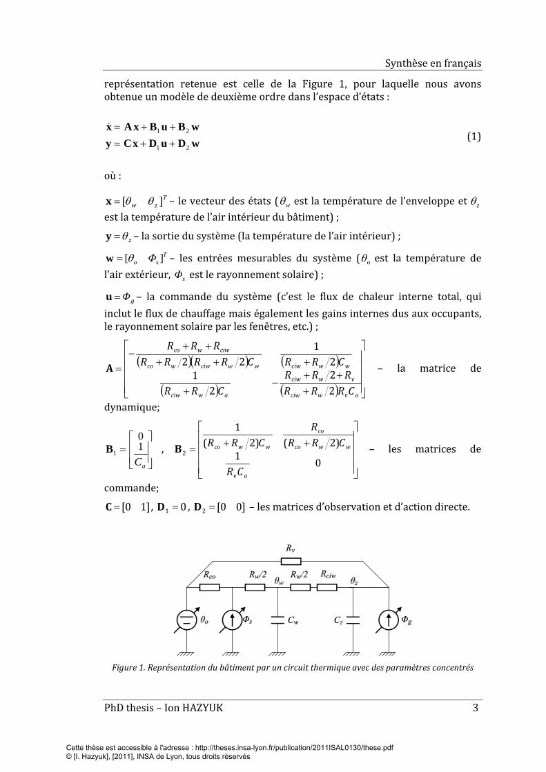
représentation retenue est celle de la Figure 1, pour laquelle nous avons obtenue un modèle de deuxième ordre dans l’espace d’états :
wDuDxCywBuBxAx
21
21
++=++=
(1)
où :
Tzw ][ θθ=x – le vecteur des états ( wθ est la température de l’enveloppe et zθ
est la température de l’air intérieur du bâtiment) ;
zθ=y – la sortie du système (la température de l’air intérieur) ; T
so Φ ][θ=w – les entrées mesurables du système ( oθ est la température de l’air extérieur, sΦ est le rayonnement solaire) ;
gΦ=u – la commande du système (c’est le flux de chaleur interne total, qui inclut le flux de chauffage mais également les gains internes dus aux occupants, le rayonnement solaire par les fenêtres, etc.) ;
( )( ) ( )
( ) ( )
+++
−+
+++++
−=
avwciw
vwciw
awciw
wwciwwwciwwco
ciwwco
CRRRRRR
CRR
CRRCRRRRRRR
22
21
21
22A – la matrice de
dynamique;
=
aC10
1B ,
++=
01)2()2(
1
2
av
wwco
co
wwco
CR
CRRR
CRRB – les matrices de
commande;
]10[=C , 01 =D , ]00[2 =D – les matrices d’observation et d’action directe.
Figure 1. Représentation du bâtiment par un circuit thermique avec des paramètres concentrés
Cette thèse est accessible à l'adresse : http://theses.insa-lyon.fr/publication/2011ISAL0130/these.pdf © [I. Hazyuk], [2011], INSA de Lyon, tous droits réservés
Synthèse en français
4 PhD thesis – Ion HAZYUK
La structure du modèle obtenu convient à une large gamme de bâtiments réels. Les modèles de deux bâtiments différents se distinguent par les valeurs de leurs paramètres. Pour obtenir les valeurs des paramètres, nous avons modélisé sous Simbad (sous l’environnement Matlab/Simulink) une maison d’environ 100 m² et nous avons utilisé la méthode d’identification des moindres carrés. Nous avons simulé le bâtiment sur une période de six mois, en appliquant à l’entré un signal binaire pseudo-aléatoire pour le flux de chaleur est des donnés statistiques pour la météo. Les donnés d’entrées/sortie ont été fragmenté en deux, afin d’avoir des échantillons différents pour l’identification des paramètres et pour leur validation.
Dans le modèle du bâtiment, nous avons utilisé comme entrée le flux de chaleur intérieur. Toutefois, le système de chauffage considéré est basé sur des radiateurs à eau. Dans ce cas, la commande du régulateur se fait sur la température ou le débit d’eau chaude et non pas sur le flux de chaleur. Nous avons exprimé la relation non-linéaire entre le flux et la température de l’eau chaude à l’entrée du radiateur.
Chapitre 3. Estimation de la charge thermique des bâtiments occupés par intermittence
Les méthodes actuelles utilisées pour l’estimation de la charge de chauffage se basent sur une hypothèse qui contredit la physique dans le cas des bâtiments occupés par intermittence.
Actuellement, les méthodes les plus précises estiment la charge de chauffage à l'aide de simulations dynamiques. Pour cela, elles utilisent un modèle dynamique qui décrit la variation de la température dans le bâtiment sous l'effet des flux de chaleur qui le traversent. Autrement dit, les flux de chaleur sont les entrées du modèle et la température est sa sortie. Ainsi, la charge de chauffage est calculée en inversant ce modèle et en imposant une température à l’air intérieur. De cette manière, on obtient la chaleur nécessaire à injecter dans le bâtiment pour que la température de l'air corresponde à celle imposée. L’hypothèse admise est que la température imposée pour le calcul est égale à la température de consigne du bâtiment. Cette hypothèse ne pose pas de problèmes quand la température de consigne est constante dans le temps. Cependant, elle n’est pas valable dans le cas des bâtiments occupés par intermittence, où la température de consigne a une évolution temporelle de type échelon. En effet, ces méthodes d’estimation calculent le flux de chaleur nécessaire à faire basculer la température du bâtiment d’un niveau à l’autre sur un pas de temps de la simulation. Or, lorsque la période d’échantillonnage est plus courte (15 min, 1 min, 30 s…), il est évident que la température de l’air dans le bâtiment n’atteindra pas sa valeur finale en un seul pas de temps. De plus, l’estimation de la charge de pointe varie en fonction de la période d’échantillonnage de la simulation. Par exemple, nous avons obtenue des variations de 22 % sur la charge de pointe lorsque la période d’échantillonnage a changé d’une heure à quinze minutes.
Cette thèse est accessible à l'adresse : http://theses.insa-lyon.fr/publication/2011ISAL0130/these.pdf © [I. Hazyuk], [2011], INSA de Lyon, tous droits réservés
Synthèse en français
PhD thesis – Ion HAZYUK 5
L’estimation de la charge de chauffage est un problème inverse qui peut être vue comme un problème de contrôle – commande.
Le fait d’avoir une température de consigne variable nécessite un contrôleur pour piloter le système de chauffage. A chaque pas de temps, le régulateur calcule le flux thermique nécessaire pour assurer les performances thermiques requises dans le bâtiment. Dans ce cas, le flux de chaleur calculé par la loi de commande représente la charge réelle du bâtiment. Par conséquence, nous proposons de transformer le problème d'estimation de la charge dans un problème de contrôle. On considère le bâtiment comme un processus thermique perturbé par les conditions météorologiques. Le régulateur calcule la commande, c’est-à-dire le flux de chaleur nécessaire, en minimisant la différence entre la consigne et la température intérieure.
Les meilleures performances de contrôle dans le bâtiment sont obtenues en utilisant une commande prédictive.
Comme chaque régulateur calcule des commandes différentes, l’intérêt est de choisir la stratégie de contrôle la plus adapté au type de performances requises. Dans les bâtiments occupés par intermittence les performances visées sont :
• la régulation : on cherche à maintenir constante la température intérieure (ou de limiter sa variation) malgré les variations de la météo et des charges internes ;
• l’asservissement : on essaye à suivre les variations de sa consigne. Il est important de relancer le chauffage à l'avance afin d'assurer le confort thermique au début de la période d'occupation.
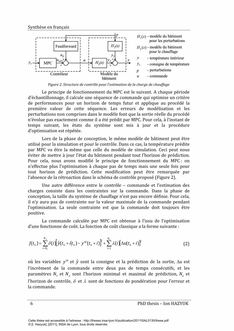
C’est dans ce but que nous avons proposé d’utiliser un schéma de contrôle composé d’un régulateur prédictif (Model Predictive Controller, MPC) et un régulateur feedforward (voir Figure 2). Le MPC est en mesure de prédire la réaction du procédé aux commandes données. En ayant connaissance de la consigne future, il peut agir de manière adéquate afin d'atteindre les meilleures performances. Ceci permet de calculer le temps de relance optimal du chauffage, toute en mettant en valeur les informations détenue au préalable sur le profile d'occupation du bâtiment. D’autre part, la technique feedforward est habituellement utilisée pour la rejection des perturbations présentes dans le système. Pour notre cas, elle permet de neutraliser l’effet de la météo sur la température intérieure. Pour calculer la commande, MPC et feedforward ont besoin d’un modèle d’ordre réduit du bâtiment.
Cette thèse est accessible à l'adresse : http://theses.insa-lyon.fr/publication/2011ISAL0130/these.pdf © [I. Hazyuk], [2011], INSA de Lyon, tous droits réservés
Synthèse en français
6 PhD thesis – Ion HAZYUK
Figure 2. Structure de contrôle pour l'estimation de la charge de chauffage
Le principe de fonctionnement du MPC est le suivant. A chaque période d’échantillonnage, il calcule une séquence de commande qui optimise un critère de performances pour un horizon de temps futur et applique au procédé la première valeur de cette séquence. Les erreurs de modélisation et les perturbations non comprises dans le modèle font que la sortie réelle du procédé n’évolue pas exactement comme il a été prédit par MPC. Pour cela, à l’instant de temps suivant, les états du système sont mis à jour et la procédure d’optimisation est répétée.
Lors de la phase de conception, le même modèle de bâtiment peut être utilisé pour la simulation et pour le contrôle. Dans ce cas, la température prédite par MPC va être la même que celle du modèle de simulation. Ceci peut nous éviter de mettre à jour l’état du bâtiment pendant tout l’horizon de prédiction. Pour cela, nous avons modifié le principe de fonctionnement du MPC : on n’effectue plus l’optimisation à chaque pas de temps mais une seule fois pour tout horizon de prédiction. Cette modification peut être remarquée par l’absence de la rétroaction dans le schéma de contrôle proposé (Figure 2).
Une autre différence entre le contrôle – commande et l’estimation des charges consiste dans les contraintes sur la commande. Dans la phase de conception, la taille du système de chauffage n’est pas encore définie. Pour cela, il n’y aura pas de contrainte sur la valeur maximale de la commande pendant l’optimisation. La seule contrainte est que la commande doit toujours être positive.
La commande calculée par MPC est obtenue à l’issu de l’optimisation d’une fonctionne de coût. La fonction de coût classique a la forme suivante :
[ ] [ ]∑∑==
+∆++−+=uy N
ik
N
Nik
spkkk ituiitytityitJ
1
22 )()()()(ˆ)()(1
λδ (2)
où les variables spy et y sont la consigne et la prédiction de la sortie, u∆ est l’incrément de la commande entre deux pas de temps consécutifs, et les paramètres 1N et yN sont l’horizon minimal et maximal de prédiction, uN et l’horizon de contrôle, δ et λ sont de fonctions de pondération pour l’erreur et la commande.
Cette thèse est accessible à l'adresse : http://theses.insa-lyon.fr/publication/2011ISAL0130/these.pdf © [I. Hazyuk], [2011], INSA de Lyon, tous droits réservés
Synthèse en français
PhD thesis – Ion HAZYUK 7
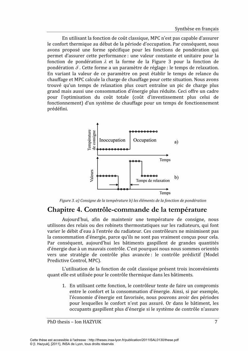
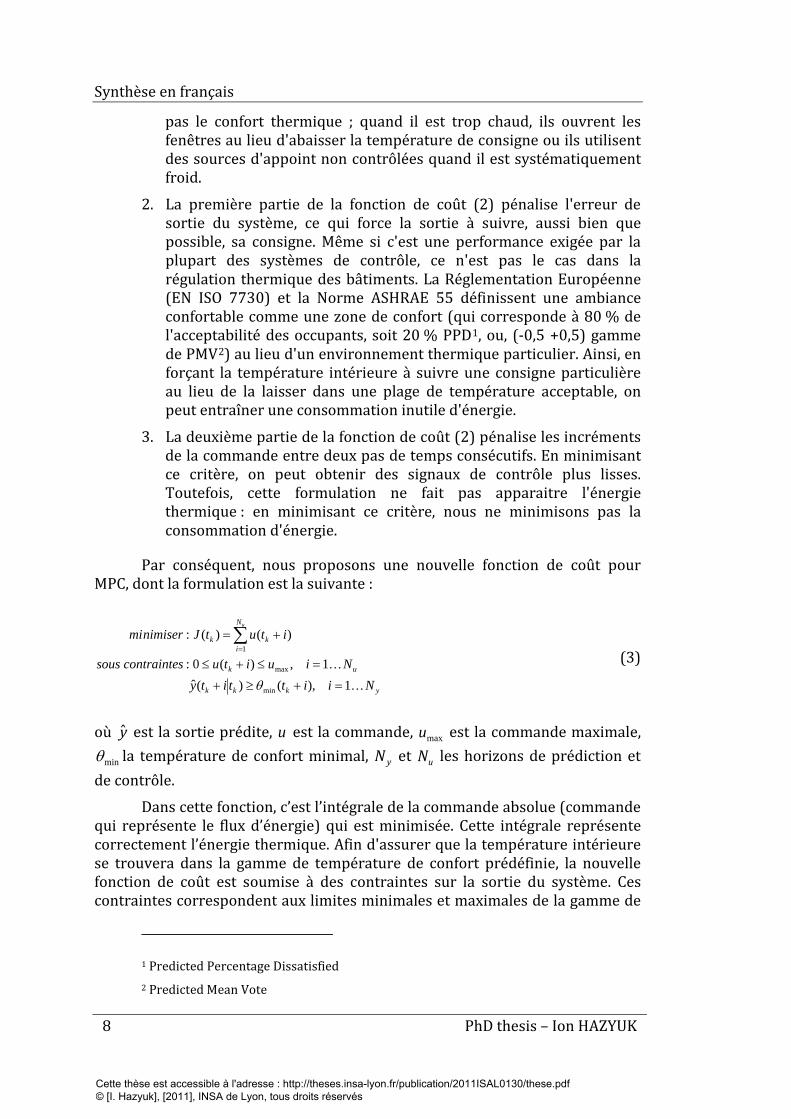
En utilisant la fonction de coût classique, MPC n’est pas capable d’assurer le confort thermique au début de la période d’occupation. Par conséquent, nous avons proposé une forme spécifique pour les fonctions de pondération qui permet d’assurer cette performance : une valeur constante et unitaire pour la fonction de pondération λ et la forme de la Figure 3 pour la fonction de pondération δ . Cette forme a un paramètre de réglage : le temps de relaxation. En variant la valeur de ce paramètre on peut établir le temps de relance du chauffage et MPC calcule la charge de chauffage pour cette situation. Nous avons trouvé qu’un temps de relaxation plus court entraîne un pic de charge plus grand mais aussi une consommation d’énergie plus réduite. Ceci offre un cadre pour l’optimisation du coût totale (coût d’investissement plus celui de fonctionnement) d’un système de chauffage pour un temps de fonctionnement prédéfini.
Figure 3. a) Consigne de la température b) les éléments de la fonction de pondération
Chapitre 4. Contrôle-commande de la température Aujourd'hui, afin de maintenir une température de consigne, nous
utilisons des relais ou des robinets thermostatiques sur les radiateurs, qui font varier le débit d'eau à l’entrée du radiateur. Ces contrôleurs ne minimisent pas la consommation d'énergie, parce qu'ils ne sont pas vraiment conçus pour cela. Par conséquent, aujourd'hui les bâtiments gaspillent de grandes quantités d'énergie due à un mauvais contrôle. C'est pourquoi nous nous sommes orientés vers une stratégie de contrôle plus avancée : le contrôle prédictif (Model Predictive Control, MPC).
L’utilisation de la fonction de coût classique présent trois inconvénients quant elle est utilisée pour le contrôle thermique dans les bâtiments.
1. En utilisant cette fonction, le contrôleur tente de faire un compromis entre le confort et la consommation d'énergie. Ainsi, si par exemple, l’économie d'énergie est favorisée, nous pouvons avoir des périodes pour lesquelles le confort n'est pas assuré. Or dans le bâtiment, les occupants gaspillent plus d'énergie si le système de contrôle n’assure
Cette thèse est accessible à l'adresse : http://theses.insa-lyon.fr/publication/2011ISAL0130/these.pdf © [I. Hazyuk], [2011], INSA de Lyon, tous droits réservés
Synthèse en français
8 PhD thesis – Ion HAZYUK
pas le confort thermique ; quand il est trop chaud, ils ouvrent les fenêtres au lieu d'abaisser la température de consigne ou ils utilisent des sources d'appoint non contrôlées quand il est systématiquement froid.
2. La première partie de la fonction de coût (2) pénalise l'erreur de sortie du système, ce qui force la sortie à suivre, aussi bien que possible, sa consigne. Même si c'est une performance exigée par la plupart des systèmes de contrôle, ce n'est pas le cas dans la régulation thermique des bâtiments. La Réglementation Européenne (EN ISO 7730) et la Norme ASHRAE 55 définissent une ambiance confortable comme une zone de confort (qui corresponde à 80 % de l'acceptabilité des occupants, soit 20 % PPD1, ou, (-0,5 +0,5) gamme de PMV2) au lieu d'un environnement thermique particulier. Ainsi, en forçant la température intérieure à suivre une consigne particulière au lieu de la laisser dans une plage de température acceptable, on peut entraîner une consommation inutile d'énergie.
3. La deuxième partie de la fonction de coût (2) pénalise les incréments de la commande entre deux pas de temps consécutifs. En minimisant ce critère, on peut obtenir des signaux de contrôle plus lisses. Toutefois, cette formulation ne fait pas apparaitre l'énergie thermique : en minimisant ce critère, nous ne minimisons pas la consommation d'énergie.
Par conséquent, nous proposons une nouvelle fonction de coût pour MPC, dont la formulation est la suivante :
ykkk
uk
N
ikk
NiittityNiuituscontraintesous
itutJnimisermiu
1),()(ˆ1,)(0:
)()(:
min
max
1
=+≥+
=≤+≤
+=∑=
θ
(3)
où y est la sortie prédite, u est la commande, maxu est la commande maximale,
minθ la température de confort minimal, yN et uN les horizons de prédiction et de contrôle.
Dans cette fonction, c’est l’intégrale de la commande absolue (commande qui représente le flux d’énergie) qui est minimisée. Cette intégrale représente correctement l’énergie thermique. Afin d'assurer que la température intérieure se trouvera dans la gamme de température de confort prédéfinie, la nouvelle fonction de coût est soumise à des contraintes sur la sortie du système. Ces contraintes correspondent aux limites minimales et maximales de la gamme de
1 Predicted Percentage Dissatisfied 2 Predicted Mean Vote
Cette thèse est accessible à l'adresse : http://theses.insa-lyon.fr/publication/2011ISAL0130/these.pdf © [I. Hazyuk], [2011], INSA de Lyon, tous droits réservés
Synthèse en français
PhD thesis – Ion HAZYUK 9
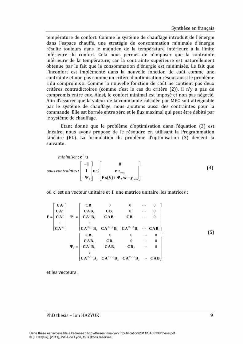
température de confort. Comme le système de chauffage introduit de l'énergie dans l'espace chauffé, une stratégie de consommation minimale d’énergie résulte toujours dans le maintien de la température intérieure à la limite inférieure du confort. Cela nous permet de n'imposer que la contrainte inférieure de la température, car la contrainte supérieure est naturellement obtenue par le fait que la consommation d'énergie est minimisée. Le fait que l’inconfort est implémenté dans la nouvelle fonction de coût comme une contrainte et non pas comme un critère d'optimisation résout aussi le problème « du compromis ». Comme la nouvelle fonction de coût ne contient pas deux critères contradictoires (comme c’est le cas du critère (2)), il n'y a pas de compromis entre eux. Ainsi, le confort minimal est imposé et non pas négocié. Afin d’assurer que la valeur de la commande calculée par MPC soit atteignable par le système de chauffage, nous ajoutons aussi des contraintes pour la commande. Elle est bornée entre zéro et le flux maximal qui peut être débité par le système de chauffage.
Etant donné que le problème d’optimisation dans l’équation (3) est linéaire, nous avons proposé de le résoudre en utilisant la Programmation Linéaire (PL). La formulation du problème d’optimisation (3) devient la suivante :
−+≤
−
−
min2
max
1 )(:
:
ywΨxFc
0u
ΨII
uc
kuscontraintesous
nimisermi T
(4)
où c est un vecteur unitaire et I une matrice unitaire, les matrices :
=
=
=
−−−
−−−
223
22
21
2222
22
2
2
113
12
11
1112
11
1
13
2
000000
000000
BACBACBACBAC
BCBACBACBCBAC
BC
Ψ
BACBACBACBAC
BCBACBACBCBAC
BC
Ψ
AC
ACACAC
F
yyy
yyyy
NNN
NNNN
(5)
et les vecteurs :
Cette thèse est accessible à l'adresse : http://theses.insa-lyon.fr/publication/2011ISAL0130/these.pdf © [I. Hazyuk], [2011], INSA de Lyon, tous droits réservés
Synthèse en français
10 PhD thesis – Ion HAZYUK
[ ][ ][ ][ ])()2()1(
)1()2()1()(
)1()2()1()(
)()3()2()1(
minminminmin y
Ty
TTTT
Ty
Ty
NkkkNkkkk
Nkukukuku
Nkykykyky
+++=
−+++=
−+++=
++++=
θθθ
ywwwww
u
y
(6)
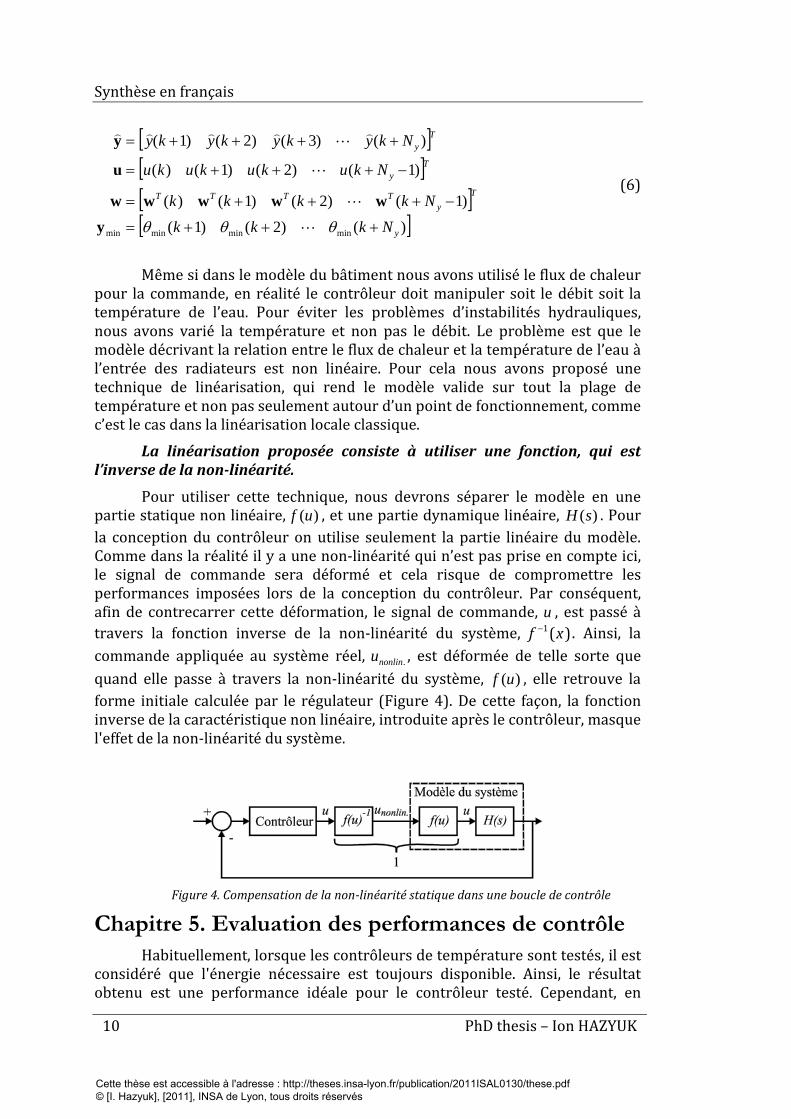
Même si dans le modèle du bâtiment nous avons utilisé le flux de chaleur pour la commande, en réalité le contrôleur doit manipuler soit le débit soit la température de l’eau. Pour éviter les problèmes d’instabilités hydrauliques, nous avons varié la température et non pas le débit. Le problème est que le modèle décrivant la relation entre le flux de chaleur et la température de l’eau à l’entrée des radiateurs est non linéaire. Pour cela nous avons proposé une technique de linéarisation, qui rend le modèle valide sur tout la plage de température et non pas seulement autour d’un point de fonctionnement, comme c’est le cas dans la linéarisation locale classique.
La linéarisation proposée consiste à utiliser une fonction, qui est l’inverse de la non-linéarité.
Pour utiliser cette technique, nous devrons séparer le modèle en une partie statique non linéaire, )(uf , et une partie dynamique linéaire, )(sH . Pour la conception du contrôleur on utilise seulement la partie linéaire du modèle. Comme dans la réalité il y a une non-linéarité qui n’est pas prise en compte ici, le signal de commande sera déformé et cela risque de compromettre les performances imposées lors de la conception du contrôleur. Par conséquent, afin de contrecarrer cette déformation, le signal de commande, u , est passé à travers la fonction inverse de la non-linéarité du système, )(1 xf − . Ainsi, la commande appliquée au système réel, .nonlinu , est déformée de telle sorte que quand elle passe à travers la non-linéarité du système, )(uf , elle retrouve la forme initiale calculée par le régulateur (Figure 4). De cette façon, la fonction inverse de la caractéristique non linéaire, introduite après le contrôleur, masque l'effet de la non-linéarité du système.
Figure 4. Compensation de la non-linéarité statique dans une boucle de contrôle
Chapitre 5. Evaluation des performances de contrôle Habituellement, lorsque les contrôleurs de température sont testés, il est
considéré que l'énergie nécessaire est toujours disponible. Ainsi, le résultat obtenu est une performance idéale pour le contrôleur testé. Cependant, en
Cette thèse est accessible à l'adresse : http://theses.insa-lyon.fr/publication/2011ISAL0130/these.pdf © [I. Hazyuk], [2011], INSA de Lyon, tous droits réservés
Synthèse en français
PhD thesis – Ion HAZYUK 11
réalité, le contrôleur agit comme une vanne: il fait varier le flux d'énergie entre la valeur minimale technologiquement possible et le maximum d'énergie disponible. Si la commande calculée est en dehors de cette plage, le système entre en saturation et la performance obtenue est dégradée. Par conséquent, afin d'obtenir des performances réalistes lors de l'essai, nous avons intégré l’algorithme de contrôle prédictif (MPC) proposé dans le chapitre précédent dans un système de gestion technique du bâtiment (GTB) qui prend en charge la gestion du système multi-sources. Les tests ont été faits en émulation et en temps réel sur un banc d'essai dédié et les performances mesurées ont été le confort thermique, la consommation d'énergie et l'usure du système. Les indices de performance obtenus pour la GTB proposée ont été comparés avec les mêmes indices obtenus pour deux autres GTB classiques basées sur des régulateurs PID. Les systèmes de GTB ont été évalués par émulation, sur le stand expérimental du CSTB dédié aux essaies des régulateurs, pendant deux périodes de cinq jours, une en hiver et une en mi saison, et pour deux zones géographiques différentes, Paris et Marseille.
La comparaison des indices de performance ont montrés que la GTB proposée a réduit l'inconfort jusqu'à 97%, a réduit la consommation d'énergie jusqu'à 18%, et a réduit le nombre de cycles de redémarrage de la pompe à chaleur jusqu'à 78% et des pompes hydrauliques auxiliaires jusqu'à 89%, par rapport aux GTB classiques.
Conclusions et perspectives Un des problèmes principaux pour une conception optimale et gestion
efficace des systèmes multi-sources (renouvelables et classiques) consiste dans l’utilisation des régulateurs non optimaux. Dans cette thèse nous proposons des régulateurs optimaux de type commande prédictive, dédiés à deux tâches différentes, qui sont l’estimation de la charge thermique et le control thermique des bâtiments.
Comme les régulateurs proposés sont basés sur le modèle du processus, nous avons d’abord obtenu un modèle du bâtiment d’ordre réduit en deux étapes. Dans une première étape nous avons modélisé le bâtiment par un circuit linéaire avec des paramètres concentrés, dont la résolution nous a donnée la structure du modèle dans l’espace d’états. Dans la deuxième étape, nous avons identifié les paramètres du modèle en utilisant la méthode des moindres carrés.
Le problème des méthodes d’estimation de la charge de chauffage consiste dans une hypothèse qui contredit la physique dans le cas des bâtiments occupés par intermittence, où la consigne est variable dans le temps. Pour cela nous avons proposé de transformer le problème d’estimation des charges dans un problème de contrôle où le régulateur calcule la charge thermique optimale du bâtiment.
Pour la régulation thermique, nous avons utilisé le contrôle prédictif, pour lequel nous avons proposé une nouvelle fonction de coût qui permet d’assurer le confort thermique avec une consommation minimale d’énergie. La nouvelle fonction de coût est formulée de telle manière qu’elle puisse être
Cette thèse est accessible à l'adresse : http://theses.insa-lyon.fr/publication/2011ISAL0130/these.pdf © [I. Hazyuk], [2011], INSA de Lyon, tous droits réservés

Synthèse en français
12 PhD thesis – Ion HAZYUK
optimisée en utilisant la Programmation Linéaire (PL). Comme la PL n’est dédiée qu’aux problèmes linéaires, nous proposons une linéarisation du modèle du bâtiment en utilisant les connaissances physiques.
Le système de contrôle proposé a été évalué et comparé avec deux GTB basées sur des régulateurs PID, à travers des critères de confort et énergétiques. L'évaluation est réalisée en émulation sur une maison individuelle de référence. Les résultats obtenus montrent que le système de contrôle – commande proposé a toujours maintenu le confort thermique dans le bâtiment, a réduit la consommation d'énergie et a réduit considérablement l'usure des pompes hydrauliques et de la pompe à chaleur présentes dans le système de chauffage.
Ainsi, nos contributions originales sont : (1) la formulation du problème d’estimation de la charge thermique sous la forme d’un problème de contrôle, (2) une nouvelle fonction de coût pour MPC qui assure le confort thermique avec une consommation minimale d'énergie, (3) la formulation du problème d’optimisation dans le cadre de la programmation linéaire, (4) l'idée de projeter le modèle du système sur une structure fixe provenant de la physique, et (5) une méthode de linéarisation qui rende un modèle valide sur toute la plage de fonctionnement.
Cette thèse est accessible à l'adresse : http://theses.insa-lyon.fr/publication/2011ISAL0130/these.pdf © [I. Hazyuk], [2011], INSA de Lyon, tous droits réservés
13
Chapter 1
Introduction
1.1 Global climate situation
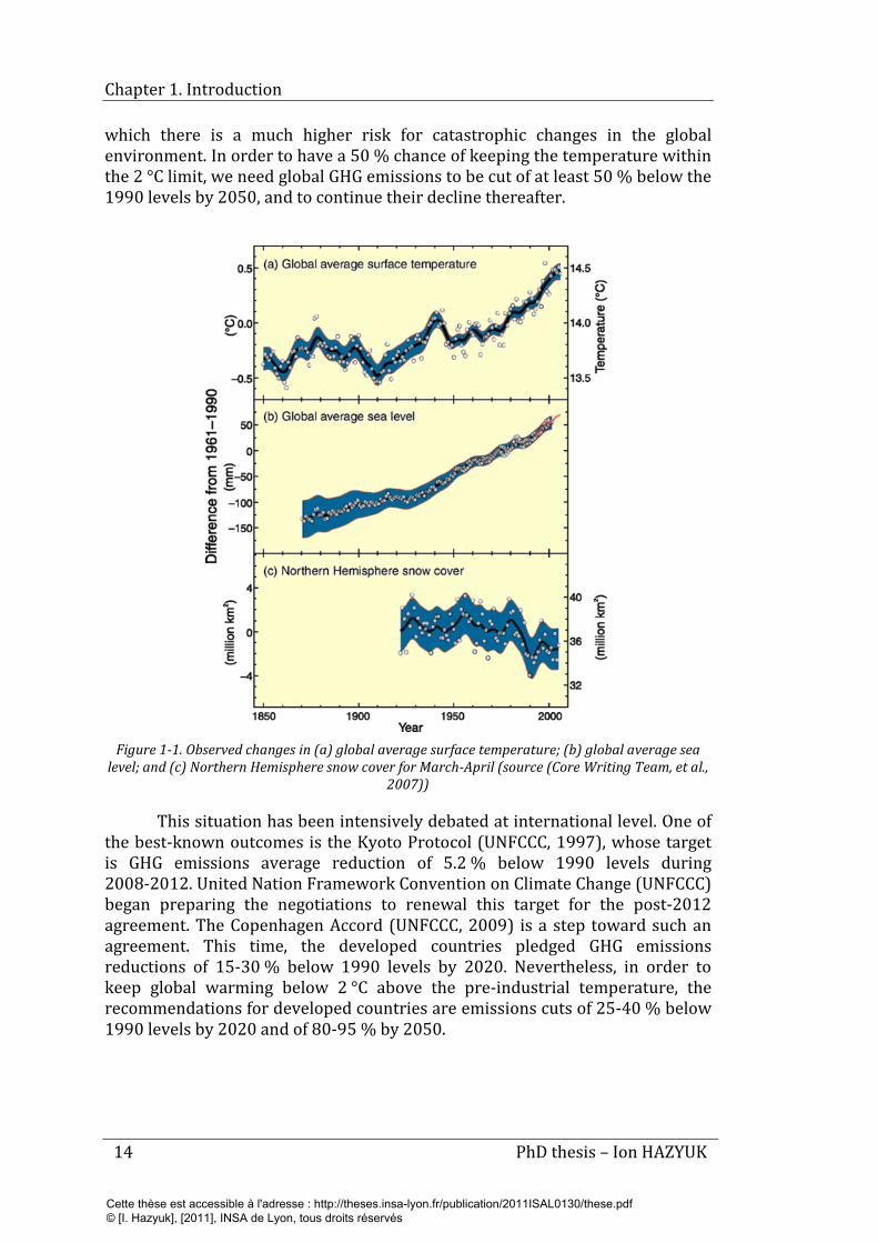
Today, our society is facing major climate changes. According to the Intergovernmental Panel on Climate Change (IPCC) report in 2007 (Core Writing Team, Pachauri & Reisinger, 2007), the alarming observations of climate change are (Figure 1-1):
• the increase of the global average temperature at the earth's surface by 0.74 °C over the past 100 years and its continuous growth since the IPCC’s first report in 1990;
• the rise of the sea level by 3.1 mm per year since 1993;
• the decrease of the arctic sea ice average surface by 2.7 % per decade since 1978.
The report highlights that the main cause of these changes is the increase by 70 % since 1970 of greenhouse gas (GHG) emissions due to human activities. In the absence of additional climate policies, an estimation of the GHG emissions evolution for the next two decades foresees an increase between 25 and 90 %. The effect of such a scenario could be the increase of the average terrestrial temperature by 0.2 °C per decade. Considering GHG emissions at the current rate, the average global temperature is projected to increase anywhere between 1.1 and 6.4 °C by the end of the 21st century and the ocean level between 18 and 59 cm. The consequences of these changes could lead to massive floods, droughts, heavy precipitation events, ocean acidification, increased frequency of heat waves and wildfires, and the list continues. A temperature increase of 2 °C above the pre-industrial times (1850-1899) is seen as the threshold beyond
Cette thèse est accessible à l'adresse : http://theses.insa-lyon.fr/publication/2011ISAL0130/these.pdf © [I. Hazyuk], [2011], INSA de Lyon, tous droits réservés
Chapter 1. Introduction
14 PhD thesis – Ion HAZYUK
which there is a much higher risk for catastrophic changes in the global environment. In order to have a 50 % chance of keeping the temperature within the 2 °C limit, we need global GHG emissions to be cut of at least 50 % below the 1990 levels by 2050, and to continue their decline thereafter.
Figure 1-1. Observed changes in (a) global average surface temperature; (b) global average sea
level; and (c) Northern Hemisphere snow cover for March-April (source (Core Writing Team, et al., 2007))
This situation has been intensively debated at international level. One of the best-known outcomes is the Kyoto Protocol (UNFCCC, 1997), whose target is GHG emissions average reduction of 5.2 % below 1990 levels during 2008-2012. United Nation Framework Convention on Climate Change (UNFCCC) began preparing the negotiations to renewal this target for the post-2012 agreement. The Copenhagen Accord (UNFCCC, 2009) is a step toward such an agreement. This time, the developed countries pledged GHG emissions reductions of 15-30 % below 1990 levels by 2020. Nevertheless, in order to keep global warming below 2 °C above the pre-industrial temperature, the recommendations for developed countries are emissions cuts of 25-40 % below 1990 levels by 2020 and of 80-95 % by 2050.
Cette thèse est accessible à l'adresse : http://theses.insa-lyon.fr/publication/2011ISAL0130/these.pdf © [I. Hazyuk], [2011], INSA de Lyon, tous droits réservés
Chapter 1. Introduction
PhD thesis – Ion HAZYUK 15
Space heating; 64,40%
Hot water preparation;
11,60%
Food preparation; 6,50%
Specific use; 17,50%
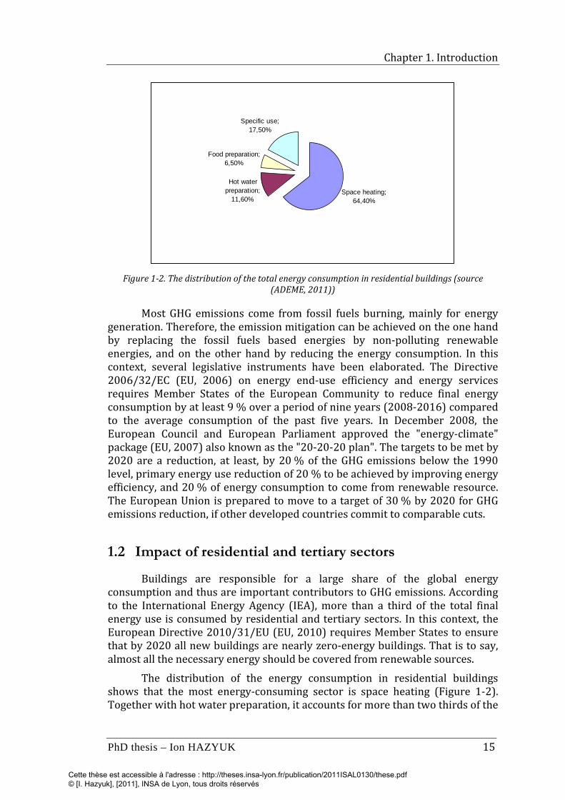
Figure 1-2. The distribution of the total energy consumption in residential buildings (source
(ADEME, 2011))
Most GHG emissions come from fossil fuels burning, mainly for energy generation. Therefore, the emission mitigation can be achieved on the one hand by replacing the fossil fuels based energies by non-polluting renewable energies, and on the other hand by reducing the energy consumption. In this context, several legislative instruments have been elaborated. The Directive 2006/32/EC (EU, 2006) on energy end-use efficiency and energy services requires Member States of the European Community to reduce final energy consumption by at least 9 % over a period of nine years (2008-2016) compared to the average consumption of the past five years. In December 2008, the European Council and European Parliament approved the "energy-climate" package (EU, 2007) also known as the "20-20-20 plan". The targets to be met by 2020 are a reduction, at least, by 20 % of the GHG emissions below the 1990 level, primary energy use reduction of 20 % to be achieved by improving energy efficiency, and 20 % of energy consumption to come from renewable resource. The European Union is prepared to move to a target of 30 % by 2020 for GHG emissions reduction, if other developed countries commit to comparable cuts.
1.2 Impact of residential and tertiary sectors
Buildings are responsible for a large share of the global energy consumption and thus are important contributors to GHG emissions. According to the International Energy Agency (IEA), more than a third of the total final energy use is consumed by residential and tertiary sectors. In this context, the European Directive 2010/31/EU (EU, 2010) requires Member States to ensure that by 2020 all new buildings are nearly zero-energy buildings. That is to say, almost all the necessary energy should be covered from renewable sources.
The distribution of the energy consumption in residential buildings shows that the most energy-consuming sector is space heating (Figure 1-2). Together with hot water preparation, it accounts for more than two thirds of the
Cette thèse est accessible à l'adresse : http://theses.insa-lyon.fr/publication/2011ISAL0130/these.pdf © [I. Hazyuk], [2011], INSA de Lyon, tous droits réservés
Chapter 1. Introduction
16 PhD thesis – Ion HAZYUK
total energy consumed in buildings. Nevertheless, space heating and hot water preparation represents the largest potential for energy savings. As far as 63 % of energy savings are achievable by using nothing but energy-efficient and low/zero-carbon heating and cooling (IEA, 2011). This implies partial replacement of the classical energy resources with renewable ones but in the same time the reduction of the building energy consumption.
1.3 Issues for an efficient consumption reduction in buildings
As building heating and domestic hot water preparation was identified as having the greatest potential for energy savings, here we are analyzing only these two tasks.
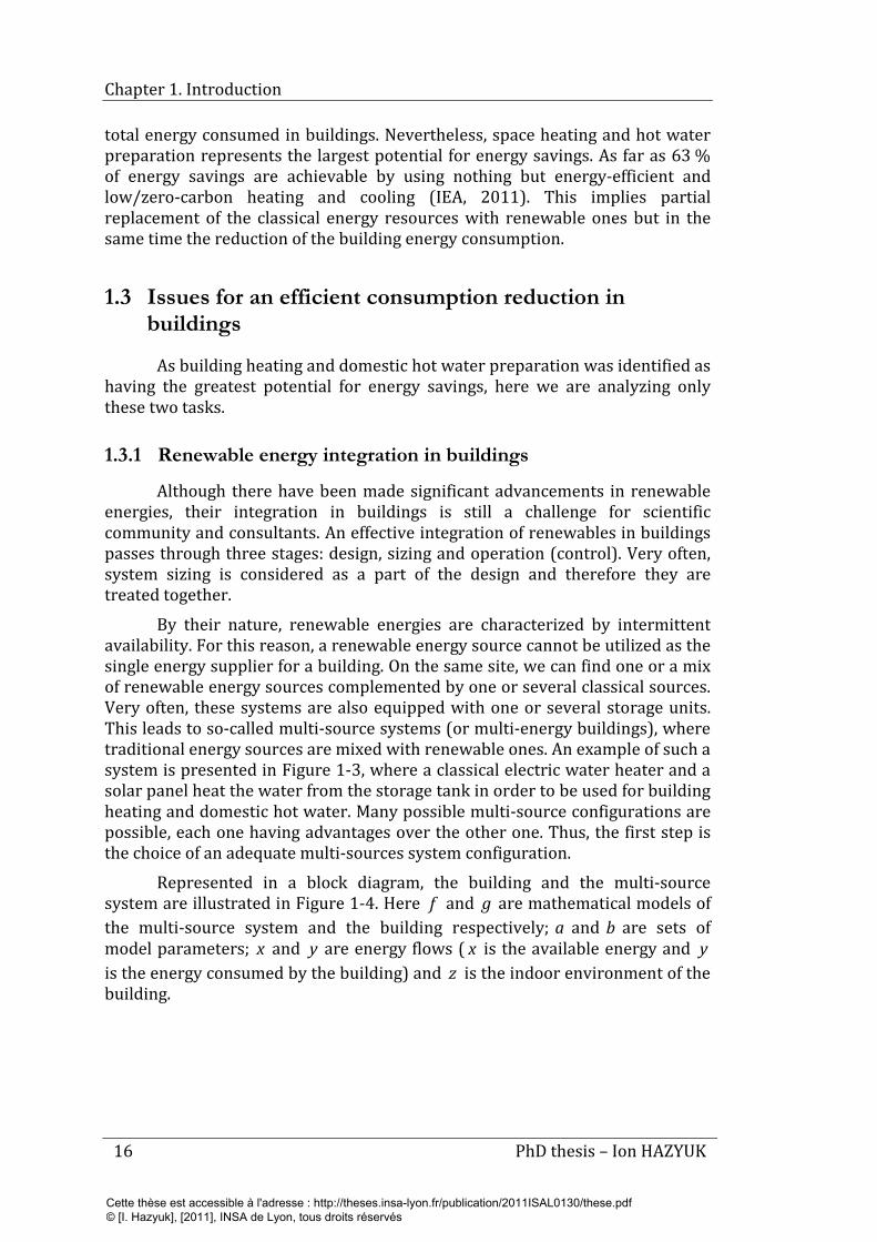
1.3.1 Renewable energy integration in buildings
Although there have been made significant advancements in renewable energies, their integration in buildings is still a challenge for scientific community and consultants. An effective integration of renewables in buildings passes through three stages: design, sizing and operation (control). Very often, system sizing is considered as a part of the design and therefore they are treated together.
By their nature, renewable energies are characterized by intermittent availability. For this reason, a renewable energy source cannot be utilized as the single energy supplier for a building. On the same site, we can find one or a mix of renewable energy sources complemented by one or several classical sources. Very often, these systems are also equipped with one or several storage units. This leads to so-called multi-source systems (or multi-energy buildings), where traditional energy sources are mixed with renewable ones. An example of such a system is presented in Figure 1-3, where a classical electric water heater and a solar panel heat the water from the storage tank in order to be used for building heating and domestic hot water. Many possible multi-source configurations are possible, each one having advantages over the other one. Thus, the first step is the choice of an adequate multi-sources system configuration.
Represented in a block diagram, the building and the multi-source system are illustrated in Figure 1-4. Here f and g are mathematical models of the multi-source system and the building respectively; a and b are sets of model parameters; x and y are energy flows ( x is the available energy and y is the energy consumed by the building) and z is the indoor environment of the building.
Cette thèse est accessible à l'adresse : http://theses.insa-lyon.fr/publication/2011ISAL0130/these.pdf © [I. Hazyuk], [2011], INSA de Lyon, tous droits réservés
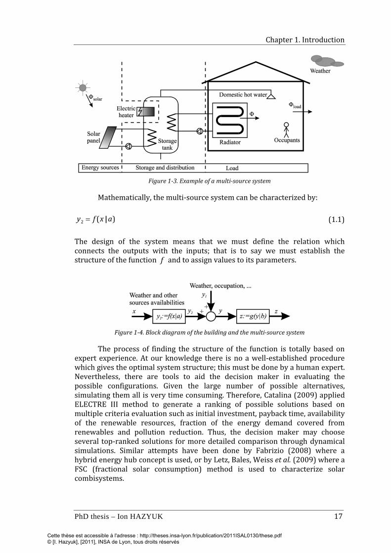
Chapter 1. Introduction
PhD thesis – Ion HAZYUK 17
Figure 1-3. Example of a multi-source system
Mathematically, the multi-source system can be characterized by:
)(2 axfy |= (1.1)
The design of the system means that we must define the relation which connects the outputs with the inputs; that is to say we must establish the structure of the function f and to assign values to its parameters.
Figure 1-4. Block diagram of the building and the multi-source system
The process of finding the structure of the function is totally based on expert experience. At our knowledge there is no a well-established procedure which gives the optimal system structure; this must be done by a human expert. Nevertheless, there are tools to aid the decision maker in evaluating the possible configurations. Given the large number of possible alternatives, simulating them all is very time consuming. Therefore, Catalina (2009) applied ELECTRE III method to generate a ranking of possible solutions based on multiple criteria evaluation such as initial investment, payback time, availability of the renewable resources, fraction of the energy demand covered from renewables and pollution reduction. Thus, the decision maker may choose several top-ranked solutions for more detailed comparison through dynamical simulations. Similar attempts have been done by Fabrizio (2008) where a hybrid energy hub concept is used, or by Letz, Bales, Weiss et al. (2009) where a FSC (fractional solar consumption) method is used to characterize solar combisystems.
Cette thèse est accessible à l'adresse : http://theses.insa-lyon.fr/publication/2011ISAL0130/these.pdf © [I. Hazyuk], [2011], INSA de Lyon, tous droits réservés
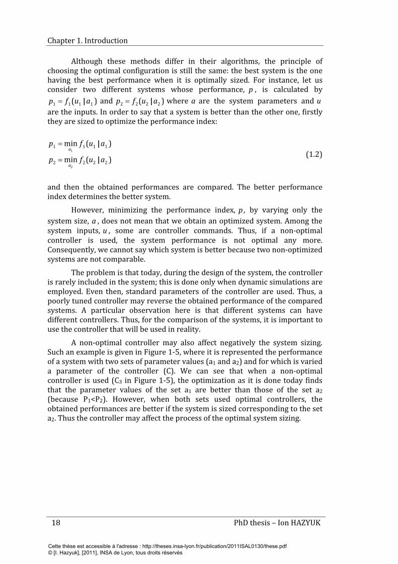
Chapter 1. Introduction
18 PhD thesis – Ion HAZYUK
Although these methods differ in their algorithms, the principle of choosing the optimal configuration is still the same: the best system is the one having the best performance when it is optimally sized. For instance, let us consider two different systems whose performance, p , is calculated by
)( 1111 aufp |= and )( 2222 aufp |= where a are the system parameters and u are the inputs. In order to say that a system is better than the other one, firstly they are sized to optimize the performance index:
)(min
)(min
2222
1111
2
1
aufp
aufp
a
a
|
|
=
= (1.2)
and then the obtained performances are compared. The better performance index determines the better system.
However, minimizing the performance index, p , by varying only the system size, a , does not mean that we obtain an optimized system. Among the system inputs, u , some are controller commands. Thus, if a non-optimal controller is used, the system performance is not optimal any more. Consequently, we cannot say which system is better because two non-optimized systems are not comparable.
The problem is that today, during the design of the system, the controller is rarely included in the system; this is done only when dynamic simulations are employed. Even then, standard parameters of the controller are used. Thus, a poorly tuned controller may reverse the obtained performance of the compared systems. A particular observation here is that different systems can have different controllers. Thus, for the comparison of the systems, it is important to use the controller that will be used in reality.
A non-optimal controller may also affect negatively the system sizing. Such an example is given in Figure 1-5, where it is represented the performance of a system with two sets of parameter values (a1 and a2) and for which is varied a parameter of the controller (C). We can see that when a non-optimal controller is used (C3 in Figure 1-5), the optimization as it is done today finds that the parameter values of the set a1 are better than those of the set a2 (because P1<P2). However, when both sets used optimal controllers, the obtained performances are better if the system is sized corresponding to the set a2. Thus the controller may affect the process of the optimal system sizing.
Cette thèse est accessible à l'adresse : http://theses.insa-lyon.fr/publication/2011ISAL0130/these.pdf © [I. Hazyuk], [2011], INSA de Lyon, tous droits réservés
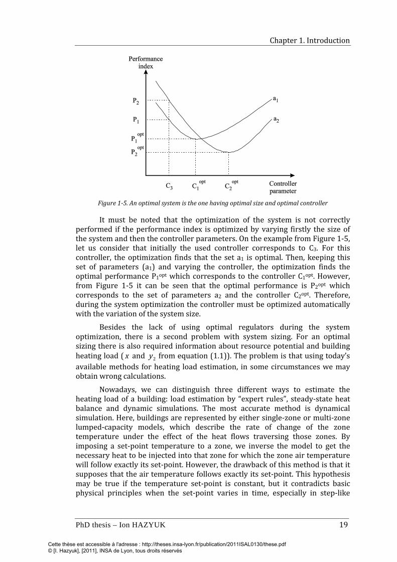
Chapter 1. Introduction
PhD thesis – Ion HAZYUK 19
Figure 1-5. An optimal system is the one having optimal size and optimal controller
It must be noted that the optimization of the system is not correctly performed if the performance index is optimized by varying firstly the size of the system and then the controller parameters. On the example from Figure 1-5, let us consider that initially the used controller corresponds to C3. For this controller, the optimization finds that the set a1 is optimal. Then, keeping this set of parameters (a1) and varying the controller, the optimization finds the optimal performance P1opt which corresponds to the controller C1opt. However, from Figure 1-5 it can be seen that the optimal performance is P2opt which corresponds to the set of parameters a2 and the controller C2opt. Therefore, during the system optimization the controller must be optimized automatically with the variation of the system size.
Besides the lack of using optimal regulators during the system optimization, there is a second problem with system sizing. For an optimal sizing there is also required information about resource potential and building heating load ( x and 2y from equation (1.1)). The problem is that using today’s available methods for heating load estimation, in some circumstances we may obtain wrong calculations.
Nowadays, we can distinguish three different ways to estimate the heating load of a building: load estimation by “expert rules”, steady-state heat balance and dynamic simulations. The most accurate method is dynamical simulation. Here, buildings are represented by either single-zone or multi-zone lumped-capacity models, which describe the rate of change of the zone temperature under the effect of the heat flows traversing those zones. By imposing a set-point temperature to a zone, we inverse the model to get the necessary heat to be injected into that zone for which the zone air temperature will follow exactly its set-point. However, the drawback of this method is that it supposes that the air temperature follows exactly its set-point. This hypothesis may be true if the temperature set-point is constant, but it contradicts basic physical principles when the set-point varies in time, especially in step-like
Cette thèse est accessible à l'adresse : http://theses.insa-lyon.fr/publication/2011ISAL0130/these.pdf © [I. Hazyuk], [2011], INSA de Lyon, tous droits réservés
Chapter 1. Introduction
20 PhD thesis – Ion HAZYUK
variations. Due to the inertia of the thermal process, the indoor temperature has a continuous evolution and not a discontinuous one, as the set-point usually has. As the simulation software generally uses discrete building models, the heating load estimated by this method strongly depends on the simulation sampling time. Thus, by using an inaccurate heating load during the evaluation of the multi-source configurations, we may loose a solution that potentially may be optimal.
The next stage of renewables integration in buildings concerns the optimal management of the sources (renewable and classical) in order to match the energy production to users’ requirements. Referring to the system description from equation (1.1), we can see that the control is an inverse problem. We need to determine which is the optimal set of inputs x , that applied for the system f with the parameters a , would give the desired output
2y :
),( 21 yafx −= (1.3)
We can see that the controller also needs information about the heating load, 2y . It must be noted, however, that the heating load, 2y , during the control is
not the same that during the system sizing. For system sizing, the heating load is computed as an optimization between the system size (that is initial investments) and corresponding energy consumption (that is operating costs). For the control, the heating load depends on the actual weather and the maximal power of the sources, which are already fixed. Therefore, for the control, we must include constraints in the calculation of the heating load.
The detail that does not resort from a classical control block-diagram is the availability of the necessary energy or power needed to control the system. The weak point of this representation is that the controller is also the energy source (Figure 1-6 a). This is not true; controllers act like a valve, regulating the energy flow between the source(s) and the consumer(s). A more explicit representation would be that from Figure 1-6 (b). When we have a source, which is able to offer anytime a constant power (though limited), in classical block-diagram (Figure 1-6 a) this limitation is highlighted by a saturation block placed between the controller and the system. In our case, however, the available energy and power varies in time and we need a controller for the sources to generate it. Thus, in order to have optimal operations, there must be some exchange of information between the controller of the sources and the controller responsible for the building thermal control. That is why in Figure 1-4 we represented separately the building and the sources and we have not embedded them together in the same “system” block, as in classical representation.
Today, the control strategies employed for the sources are relays, usually based on differential control (Suter, Letz, Weiss & Inäbnit, 2000). There is a lack of optimal controllers for the sources, which would take into account prediction of the heating load, meteorological forecast and wear and tear of the equipment.
Cette thèse est accessible à l'adresse : http://theses.insa-lyon.fr/publication/2011ISAL0130/these.pdf © [I. Hazyuk], [2011], INSA de Lyon, tous droits réservés

Chapter 1. Introduction
PhD thesis – Ion HAZYUK 21
Figure 1-6. Control scheme representations: a) the controller seems to be the source; b) the
controller is a valve
1.3.2 Building energy consumption reduction
A maximal reduction of fossil fuels energy use is not achievable only through optimal management of the renewable sources. The management of energy consumers is at least as much important. The control system of the sources will mainly react to the energy demand. Therefore, if the energy demand is not optimal, i.e. it is not controlled by an optimal regulator, the control system of the sources will not be able to reduce the energy consumption at its maximal potential.
In order to maintain a comfortable thermal environment, today the most common solution is to use relays or thermostatic valves on radiators (TVR) (Peeters, Van der Veken, Hens, Helsen & D'Haeseleer, 2008). They vary the inlet water flow rate according to an on-off scenario in the case of thermostats, or continuously in the case of TVR. However, these controllers waste much energy and wear the elements.
Obviously, the best performance can be achieved only when we completely understand how the system works (i.e. have its model) and know in advance which will be the requirements and environmental conditions (i.e. future set-point and weather forecast). These characteristics turn by default the optimal control into predictive control. Model Predictive Control (MPC) is one of the best solutions for building thermal control in intermittently heated buildings, because:
1. It is able to use the occupancy schedule and weather forecasts for optimal temperature control.
2. It optimizes both comfort and energetic criteria.
3. It is able to handle implicitly the constraints in Multi-Input Multi-Output (MIMO) systems.
4. It is able to predict the heating restart time in order to reach the thermal comfort just before the occupation period begins.
In order to calculate the command, MPC minimizes a cost function, which is usually defined as:
Cette thèse est accessible à l'adresse : http://theses.insa-lyon.fr/publication/2011ISAL0130/these.pdf © [I. Hazyuk], [2011], INSA de Lyon, tous droits réservés
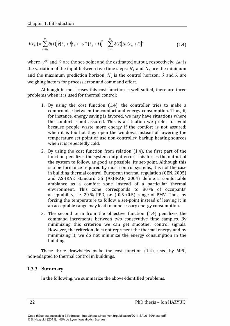
Chapter 1. Introduction
22 PhD thesis – Ion HAZYUK
[ ] [ ]∑∑==
+∆++−+=uN
ik
N
Nik
spkkk ituiitytityitJ
1
22 )()()()(ˆ)()(2
1
λδ (1.4)
where spy and y are the set-point and the estimated output, respectively; u∆ is the variation of the input between two time steps; 1N and 2N are the minimum and the maximum prediction horizon; uN is the control horizon; δ and λ are weighing factors for process error and command effort.
Although in most cases this cost function is well suited, there are three problems when it is used for thermal control:
1. By using the cost function (1.4), the controller tries to make a compromise between the comfort and energy consumption. Thus, if, for instance, energy saving is favored, we may have situations where the comfort is not assured. This is a situation we prefer to avoid because people waste more energy if the comfort is not assured; when it is too hot they open the windows instead of lowering the temperature set-point or use non-controlled backup heating sources when it is repeatedly cold.
2. By using the cost function from relation (1.4), the first part of the function penalizes the system output error. This forces the output of the system to follow, as good as possible, its set-point. Although this is a performance required by most control systems, it is not the case in building thermal control. European thermal regulation (CEN, 2005) and ASHRAE Standard 55 (ASHRAE, 2004) define a comfortable ambiance as a comfort zone instead of a particular thermal environment. This zone corresponds to 80 % of occupants’ acceptability, i.e. 20 % PPD, or, (-0.5 +0.5) range of PMV. Thus, by forcing the temperature to follow a set-point instead of leaving it in an acceptable range may lead to unnecessary energy consumption.
3. The second term from the objective function (1.4) penalizes the command increments between two consecutive time samples. By minimizing this criterion we can get smoother control signals. However, the criterion does not represent the thermal energy and by minimizing it, we do not minimize the energy consumption in the building.
These three drawbacks make the cost function (1.4), used by MPC, non-adapted to thermal control in buildings.
1.3.3 Summary
In the following, we summarize the above-identified problems.
Cette thèse est accessible à l'adresse : http://theses.insa-lyon.fr/publication/2011ISAL0130/these.pdf © [I. Hazyuk], [2011], INSA de Lyon, tous droits réservés
Chapter 1. Introduction
PhD thesis – Ion HAZYUK 23
1. The comparison of two different multisource configurations is not performed correctly. The system is rarely optimally sized and the controller is not always included in the performance estimation. Even when it is included, its parameters are not optimized. Thus, the two systems cannot be correctly compared.
2. In the dynamic simulation methods used nowadays, the heating load of the building is wrongly estimated if intermittent heating is employed. Its calculation is done by considering that the indoor temperature is equal to its set-point, which is a non-physical assumption.
3. There is not an optimal control strategy for the multisource system control, which would consider prediction of the heating load, meteorological, forecast and wear and tear of the equipment.
4. The cost function used in MPC is inadequately formulated for thermal control. It makes a trade-off between comfort and energy savings, it consumes more energy to maintain the temperature at the set-point instead of maintaining it in a comfort range and it does not minimize the energy consumption.
1.4 The proposed approach
In §1.3 we identified four problems for an efficient reduction of fossil energy consumption in buildings by optimizing the control. In this section, we briefly outline the proposed solutions for some of these problems.
1.4.1 Thermal load estimation
In buildings, heating systems are generally driven by controllers. At each sampling time, the controller calculates the power at which the heating system operates. Thus, during the operation, that power represents actually the real heating load of the building. Hence the idea to transform the heating load estimation problem into a control problem. We consider the building as a thermal process, disturbed by weather conditions and occupants, where we have to control the indoor temperature by introducing a heat flow into the building. By simulating a control algorithm on this process, we get the evolution of the necessary heat flow that will assure in the building the thermal performances imposed during the controller design. The resulted heat flow represents the heating load of the building. Thus, the problem of heating load estimation becomes a problem of choice of the control algorithm and finding the command given by this algorithm.
Our approach is to divide the heating load estimation in two parts. First, we calculate the heating load that would totally neutralize the effect of the weather (outdoor temperature and solar radiation). For this purpose, we will use feed-forward algorithm; its role is to calculate when and how much heat is needed to be introduced in the building in order to reject the disturbance effect.
Cette thèse est accessible à l'adresse : http://theses.insa-lyon.fr/publication/2011ISAL0130/these.pdf © [I. Hazyuk], [2011], INSA de Lyon, tous droits réservés
Chapter 1. Introduction
24 PhD thesis – Ion HAZYUK
Then we calculate the load that would force the indoor temperature to follow as close as possible the set-point. For this task we will employ MPC, but without constraints on the maximal power.
Besides the fact that it must be realistic, it is preferable to have an optimal heating load, i.e. a wise ratio between the maximal load and energy consumption. Thus, the employed controller has to be optimal. Given the fact that we are in design stage, we have in advance information about the building occupation schedule. This permits us to use a predictive control strategy, which is in fact an open loop optimisation procedure.
Both MPC and feed-forward are model-based algorithms; therefore, we need the dynamic model of the process, which is the building. A rigorous thermal dynamic model of a building has an elevated order and depends on plenty of building elements. However, that complicated model can be significantly reduced while maintaining an accurate reproduction of the indoor temperature behavior. Our approach is to determine the model structure using a lumped capacity representation and identify the model parameters using least squares identification method.
1.4.2 A new cost function for MPC
The cost function optimized within MPC has to reflect the desired performances of the thermal controller. The performance we are looking for is to keep the indoor temperature within the comfort temperature limits and in the same time to minimize the energy consumption.
Thus, for the energy consumption minimization we propose the cost function, J , (equation (1.5)). Here the command, u , represents the heat flux, and in this case the cost function, J , is a correct formulation of the consumed thermal energy. In order to satisfy the comfort temperature, we add constraints on the system output, (1.6). As the output of the system is the indoor temperature, the constraints means that the output temperature is forced to vary between the imposed bounds. However, as we are dealing only with a heating system, we do not take into account the upper bound of the comfort temperature. Therefore, the constraint from (1.6) is defined only for the lower temperature bound. In addition to this constraint, we impose another one on the command signal, equation (1.7). This constraint will limit the command to achievable values by the heating system.
Thus, the proposed cost function for thermal control in buildings minimizes the heat flux subject to constraints on the indoor temperature and the heat flux itself:
∑= uJ (1.5)
Cette thèse est accessible à l'adresse : http://theses.insa-lyon.fr/publication/2011ISAL0130/these.pdf © [I. Hazyuk], [2011], INSA de Lyon, tous droits réservés
Chapter 1. Introduction
PhD thesis – Ion HAZYUK 25
minˆ θ≥y (1.6)
max0 uu ≤≤ (1.7)
1.5 Outline of the thesis
In this introductive chapter, we presented the climate change problem, which is related to energy consumption. Along with this, we highlighted the solutions proposed by scientists, which in their opinion can ameliorate the climate situation. We identified four issues that are impeding the path to the proposed solutions and, for some of them, we described briefly the proposed approach.
Chapter 2 proposes a possible solution for building thermal behaviour modelling. This model is needed for thermal controller and heating load assessment. The model is obtained in two steps: first, the model structure is identified from a linear circuit with lumped parameters representation of the building and then, model parameters are identified by experimental identification using least squares algorithm. Some model characteristics are nonlinear due to convective and radiative transfer. Therefore, we show a way to identify and represent the model as a split of two blocks – linear and nonlinear, which will be used later for the control. This information, based on the physical knowledge, will be used to linearize the system model, which will ameliorate the control performance compared to classical model linearization. Here the building is represented by its white-box model and implemented in dedicated simulation software (Husaunndee, Lahrech, Vaezi-Nejad & Visier, 1997). Therefore the experimental identification is done for this simulated building and not a real one.
In chapter 3, we present the proposed solution for heating load assessment. We show an example of the heating load calculation for intermittent building occupation and indicate the issues in the assessed load using actual algorithms. Then, we show that the heat load assessment can be treated as a control problem and split the problem in two parts. In the first part, we calculate the heating load that would neutralize the effect of the meteorological conditions, i.e. outdoor temperature and solar radiation, by using a feed-forward control algorithm. In the second part, we calculate the heating load necessary to force the indoor temperature to follow the set-point temperature. This is done by using Dynamic Matrix Control, which is a variation of the Model Predictive Control.
Chapter 4 treats the problem of the optimal thermal control in buildings. Here we highlight the drawbacks of the current control algorithms and especially of the cost function currently used in MPC. Then we propose a new cost function which is adapted for thermal control and which assures the
Cette thèse est accessible à l'adresse : http://theses.insa-lyon.fr/publication/2011ISAL0130/these.pdf © [I. Hazyuk], [2011], INSA de Lyon, tous droits réservés
Chapter 1. Introduction
26 PhD thesis – Ion HAZYUK
minimal thermal comfort with minimal energy consumption. We show how to formulate the optimization problem in order to use Linear Programming for solving efficiently the optimization problem. Here, we also show how we can liniarize the building model by using the nonlinear characteristic, identified in chapter 2.
In chapter 5, we propose a Building Energy Management System, based on the proposed MPC for temperature control. Here we present the multi-source heating system and two reference PID-based management systems, which are the most advanced control systems that can be found today in practice. We compare the simulation results of the three management systems using different comfort and consumption indicators. Another aspect that we are regarding is the wear and tear of some sensitive elements of the multisource.
Finally, the manuscript is concluded by resuming the identified issues and the proposed solutions treated in the thesis, along with a critical view of the proposed solutions.
Cette thèse est accessible à l'adresse : http://theses.insa-lyon.fr/publication/2011ISAL0130/these.pdf © [I. Hazyuk], [2011], INSA de Lyon, tous droits réservés
Chapter 1. Introduction
PhD thesis – Ion HAZYUK 27
Bibliography
ADEME (2011). Chiffres clés du bâtiment – énergie – environnement (2010 ed.): Agence de l'Environnement et de la Maîtrise de l'Energie.
ASHRAE (2004). ASHRAE Standard 55-2004: Thermal environmental conditions for human occupancy. Atlanta, GA: American Society of Heating, Refrigerating, and Air-Conditioning Engineers.
Catalina, T. (2009). Estimation of residential buildings energy consumptions and analysis of renewable energy systems using a multicriteria decision methodology. Ph.D. thesis, INSA-Lyon, Lyon.
CEN (2005). EN ISO 7730:2005: Ergonomics of the thermal environment - Analytical determination and interpretation of thermal comfort using calculation of the PMV and PPD indices and local thermal comfort criteria. Brussels, Belgium: European Committee for Standardization.
Core Writing Team, Pachauri, R. K. & Reisinger, A. (2007). Climate Change 2007: Synthesis Report. Contribution of Working Groups I, II and III to the Fourth Assessment Report of the Intergovernmental Panel on Climate Change. Geneva, Switzerland: Intergovernmental Panel on Climate Change.
EU (2006). Directive 2006/32/EC on energy end-use efficiency and energy services. Official Journal of the European Union, L 114, 27.4.2006, pp. 64-85.
EU (2007). Communication from the commission to the European Council and European Parlament. An energy policy for Europe. Brussels, com(2007) 1 final.
EU (2010). Directive 2010/31/UE on the energy performance of buildings. Official Journal of the European Union, L 153, 18.6.2010, pp. 13-35.
Fabrizio, E. (2008). Modelling of multi-energy systems in buildings. Ph.D. thesis, INSA-Lyon, Lyon.
Husaunndee, A., Lahrech, R., Vaezi-Nejad, H. & Visier, J. C. (1997). SIMBAD: A simulation toolbox for the design and test of HVAC control systems. In: 5th international IBPSA conference, September 8-10, 1997, Prague, Czech Republic.
IEA (2011). Technology roadmap. Energy-efficient buildings: Heating and cooling equipment: International Energy Agency.
Letz, T., Bales, C. & Perers, B. (2009). A new concept for combisystems characterisation: The FSC method. Solar Energy, 83, 1540-1549.
Peeters, L., Van der Veken, J., Hens, H., Helsen, L. & D'Haeseleer, W. (2008). Control of heating systems in residential buildings: Current practice. Energy and Buildings, 40(8), 1446-1455.
Cette thèse est accessible à l'adresse : http://theses.insa-lyon.fr/publication/2011ISAL0130/these.pdf © [I. Hazyuk], [2011], INSA de Lyon, tous droits réservés

Chapter 1. Introduction
28 PhD thesis – Ion HAZYUK
Suter, J.-M., Letz, T., Weiss, W. & Inäbnit, J. (Eds.). (2000). Solar Combisystems in Austria, Denmark, Finland, France, Germany, Sweden, Switzerland, the Netherlands and the USA, Overview 2000. IEA SHC – TASK 26. Bern.
UNFCCC (1997). Kyoto Protocol to the United Nations Framework Convention on Climate Change. Kyoto, Japan.
UNFCCC (2009). Copenhagen Accord. Copenhage, Denmark.
Cette thèse est accessible à l'adresse : http://theses.insa-lyon.fr/publication/2011ISAL0130/these.pdf © [I. Hazyuk], [2011], INSA de Lyon, tous droits réservés
29
Chapter 2
Dynamic modeling of a building
Optimal control algorithms are model based techniques. Therefore, an optimal thermal controller needs the dynamic model of the building. The building model is of particular importance for Model Predictive Control (MPC), which is one of the best solutions available. MPC is able to use the occupancy schedule and weather forecasts for optimal temperature control. Therefore, in this chapter, we treat the problems related to building modeling and model parameters identification. In order to provide a robust model, we proceed in two stages. First, we use physical knowledge to determine the structure of low-order thermal network model of a mono-zone building. Then, we apply least squares method to experimental identification of the model parameters. During the physical analysis, we reveal some model nonlinearity and show how to identify experimentally the model parameters, without resorting to the nonlinear system theory. Later in the thesis, we use the identified model for MPC.
2.1 Introduction
Today, the role of the simulation in engineering is becoming increasingly important. Basically, before creating a new system, engineers simulate its behavior to assess its performance or detect possible faults in the system design. Therefore, on the market there are many dedicated software to simulate building systems, e.g. CODYBA (Noël, Roux & Schneider, 2001), TRNSYS (Klein et al., 2004), Comfie (Peuportier & Sommereux, 1994), ESP-R (Clarke, 2001), ENERGY + (EnergyPlus, 2009) or Simbad (Husaunndee, Lahrech, Vaezi-Nejad & Visier, 1997).
In order to simulate the thermal behavior of a building, the software uses models based on first principles and constitutive laws of thermodynamics. These models aggregate all the physical components of a building in a system of
Cette thèse est accessible à l'adresse : http://theses.insa-lyon.fr/publication/2011ISAL0130/these.pdf © [I. Hazyuk], [2011], INSA de Lyon, tous droits réservés
Chapter 2. Dynamic modeling of a building
30 PhD thesis – Ion HAZYUK
algebraic and differential equations of a very high order. Due to their high order, these models are not appropriate to develop control algorithms. For the purpose of control, it is preferable to have linear and low-order dynamic models that can approximate the system behavior in the frequency domain of interest. These low order models can be achieved by black-box identification, model reduction, or by lumped parameter representations.
A way to get a low-order model of the building is to apply black-box identification on the real system (Ríos-Moreno, Trejo-Perea, Castañeda-Miranda, Hernández-Guzmán & Herrera-Ruiz, 2007). This technique, which requires very few information about the system to be modeled, consists of analyzing the input-output data of the process. It finds the model structure and its parameter values. However, even if we get acceptable performances of the estimated models, the model parameters do not have any physical meaning and, very often, their values contradict physical phenomena; for example, we can have complex conjugated poles though, a physical analysis shows that they do not exist in thermal model of a building (Mejri, Palomo Del Barrio & Ghrab-Morcos, 2011). Moreover, when the system has some nonlinear behavior, black-box identification yields a model valid only around the operating point where it was identified. For other operating points, the model will be invalid and consequently the control performances will not be as expected; this was the reason of using online recursive identification in conjunction with adaptive controllers (Boaventura Cunha, Couto & Ruano, 1997).
Another way to obtain a low-order approximation of the building is by using model size reduction methods (Palomo Del Barrio, Lefebvre, Behar & Bailly, 2000). These techniques drastically reduce the order of a model obtained by spatial discretization of the heat transfer equations. It gives us the reduced number of equations and the parameter values by purely mathematical manipulations. Usually, in buildings, the initial (high-order) model can have hundreds or thousands of differential equations and by applying this technique, we can reduce their number to less than ten (Sempey, Inard, Ghiaus & Allery, 2009). However, in order to apply this technique we need the initial detailed model of the system. This one is obtained by applying physical knowledge to the detailed description of the building, which is not a trivial task. Moreover, for existing buildings we do not even have all the details needed to express the initial model.
A third possibility to obtain low-order models is to use lumped parameters, which can be seen as a combination between the two previous methods. Here we find directly the low order model structure by applying basic physical principles and the parameter values are estimated by using identification techniques on the defined model structure (Coley & Penman, 1996; Jiménez, Madsen & Andersen, 2008; Madsen & Holst, 1995). In literature, it is also known as gray-box model. The advantage of this approach is that by using basic physical knowledge we can represent a class of nonlinear systems using only the linear system theory (Ghiaus, Chicinas & Inard, 2007) and we can get a robust parameter identification by bounding some parameters to keep
Cette thèse est accessible à l'adresse : http://theses.insa-lyon.fr/publication/2011ISAL0130/these.pdf © [I. Hazyuk], [2011], INSA de Lyon, tous droits réservés
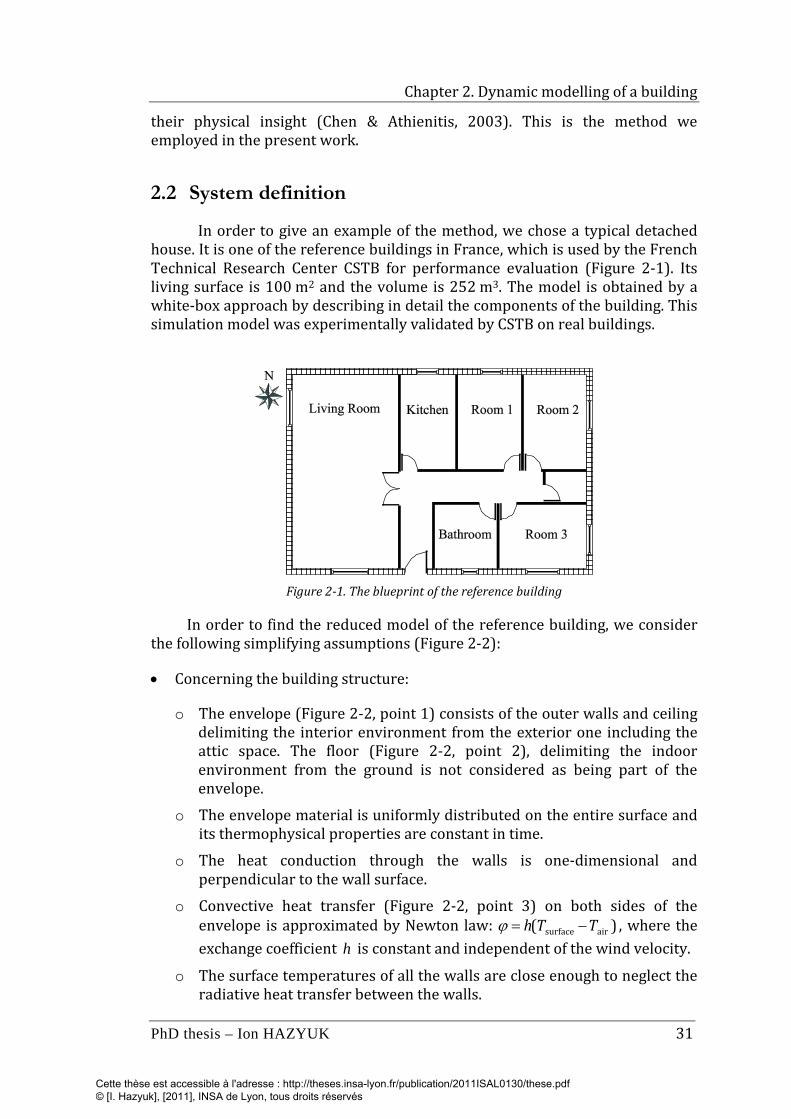
Chapter 2. Dynamic modelling of a building
PhD thesis – Ion HAZYUK 31
their physical insight (Chen & Athienitis, 2003). This is the method we employed in the present work.
2.2 System definition
In order to give an example of the method, we chose a typical detached house. It is one of the reference buildings in France, which is used by the French Technical Research Center CSTB for performance evaluation (Figure 2-1). Its living surface is 100 m2 and the volume is 252 m3. The model is obtained by a white-box approach by describing in detail the components of the building. This simulation model was experimentally validated by CSTB on real buildings.
Figure 2-1. The blueprint of the reference building
In order to find the reduced model of the reference building, we consider the following simplifying assumptions (Figure 2-2):
• Concerning the building structure:
o The envelope (Figure 2-2, point 1) consists of the outer walls and ceiling delimiting the interior environment from the exterior one including the attic space. The floor (Figure 2-2, point 2), delimiting the indoor environment from the ground is not considered as being part of the envelope.
o The envelope material is uniformly distributed on the entire surface and its thermophysical properties are constant in time.
o The heat conduction through the walls is one-dimensional and perpendicular to the wall surface.
o Convective heat transfer (Figure 2-2, point 3) on both sides of the envelope is approximated by Newton law: )( airsurface TTh −=ϕ , where the exchange coefficient h is constant and independent of the wind velocity.
o The surface temperatures of all the walls are close enough to neglect the radiative heat transfer between the walls.
Cette thèse est accessible à l'adresse : http://theses.insa-lyon.fr/publication/2011ISAL0130/these.pdf © [I. Hazyuk], [2011], INSA de Lyon, tous droits réservés
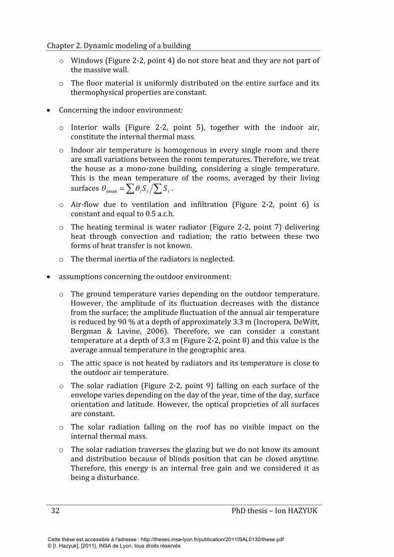
Chapter 2. Dynamic modeling of a building
32 PhD thesis – Ion HAZYUK
o Windows (Figure 2-2, point 4) do not store heat and they are not part of the massive wall.
o The floor material is uniformly distributed on the entire surface and its thermophysical properties are constant.
• Concerning the indoor environment:
o Interior walls (Figure 2-2, point 5), together with the indoor air, constitute the internal thermal mass.
o Indoor air temperature is homogenous in every single room and there are small variations between the room temperatures. Therefore, we treat the house as a mono-zone building, considering a single temperature. This is the mean temperature of the rooms, averaged by their living surfaces ∑∑= iii SSθθmean .
o Air-flow due to ventilation and infiltration (Figure 2-2, point 6) is constant and equal to 0.5 a.c.h.
o The heating terminal is water radiator (Figure 2-2, point 7) delivering heat through convection and radiation; the ratio between these two forms of heat transfer is not known.
o The thermal inertia of the radiators is neglected.
• assumptions concerning the outdoor environment:
o The ground temperature varies depending on the outdoor temperature. However, the amplitude of its fluctuation decreases with the distance from the surface; the amplitude fluctuation of the annual air temperature is reduced by 90 % at a depth of approximately 3.3 m (Incropera, DeWitt, Bergman & Lavine, 2006). Therefore, we can consider a constant temperature at a depth of 3.3 m (Figure 2-2, point 8) and this value is the average annual temperature in the geographic area.
o The attic space is not heated by radiators and its temperature is close to the outdoor air temperature.
o The solar radiation (Figure 2-2, point 9) falling on each surface of the envelope varies depending on the day of the year, time of the day, surface orientation and latitude. However, the optical proprieties of all surfaces are constant.
o The solar radiation falling on the roof has no visible impact on the internal thermal mass.
o The solar radiation traverses the glazing but we do not know its amount and distribution because of blinds position that can be closed anytime. Therefore, this energy is an internal free gain and we considered it as being a disturbance.
Cette thèse est accessible à l'adresse : http://theses.insa-lyon.fr/publication/2011ISAL0130/these.pdf © [I. Hazyuk], [2011], INSA de Lyon, tous droits réservés
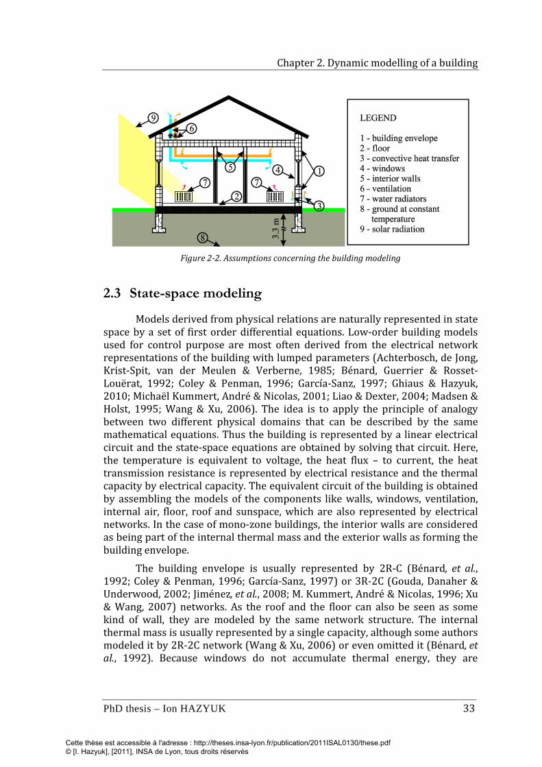
Chapter 2. Dynamic modelling of a building
PhD thesis – Ion HAZYUK 33
Figure 2-2. Assumptions concerning the building modeling
2.3 State-space modeling
Models derived from physical relations are naturally represented in state space by a set of first order differential equations. Low-order building models used for control purpose are most often derived from the electrical network representations of the building with lumped parameters (Achterbosch, de Jong, Krist-Spit, van der Meulen & Verberne, 1985; Bénard, Guerrier & Rosset-Louërat, 1992; Coley & Penman, 1996; García-Sanz, 1997; Ghiaus & Hazyuk, 2010; Michaël Kummert, André & Nicolas, 2001; Liao & Dexter, 2004; Madsen & Holst, 1995; Wang & Xu, 2006). The idea is to apply the principle of analogy between two different physical domains that can be described by the same mathematical equations. Thus the building is represented by a linear electrical circuit and the state-space equations are obtained by solving that circuit. Here, the temperature is equivalent to voltage, the heat flux – to current, the heat transmission resistance is represented by electrical resistance and the thermal capacity by electrical capacity. The equivalent circuit of the building is obtained by assembling the models of the components like walls, windows, ventilation, internal air, floor, roof and sunspace, which are also represented by electrical networks. In the case of mono-zone buildings, the interior walls are considered as being part of the internal thermal mass and the exterior walls as forming the building envelope.
The building envelope is usually represented by 2R-C (Bénard, et al., 1992; Coley & Penman, 1996; García-Sanz, 1997) or 3R-2C (Gouda, Danaher & Underwood, 2002; Jiménez, et al., 2008; M. Kummert, André & Nicolas, 1996; Xu & Wang, 2007) networks. As the roof and the floor can also be seen as some kind of wall, they are modeled by the same network structure. The internal thermal mass is usually represented by a single capacity, although some authors modeled it by 2R-2C network (Wang & Xu, 2006) or even omitted it (Bénard, et al., 1992). Because windows do not accumulate thermal energy, they are
Cette thèse est accessible à l'adresse : http://theses.insa-lyon.fr/publication/2011ISAL0130/these.pdf © [I. Hazyuk], [2011], INSA de Lyon, tous droits réservés
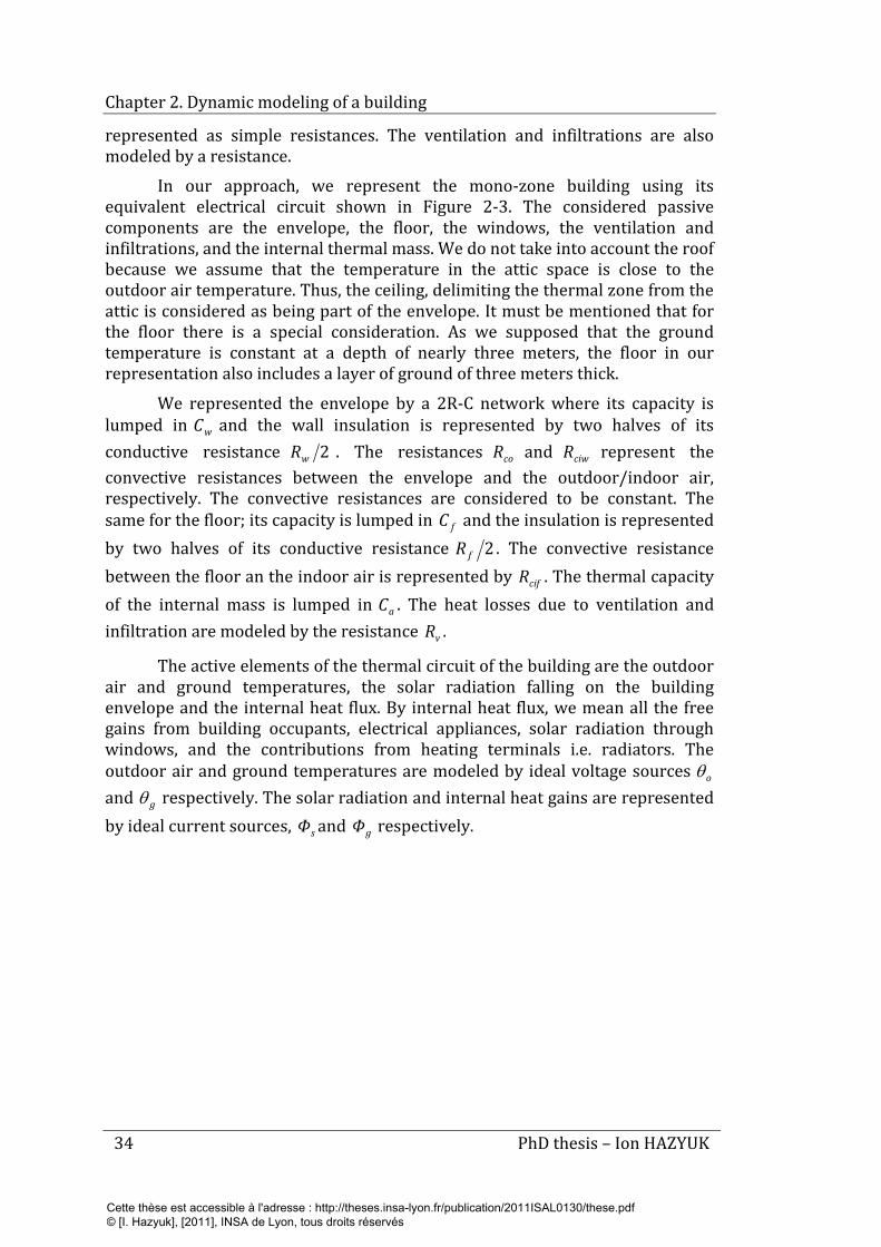
Chapter 2. Dynamic modeling of a building
34 PhD thesis – Ion HAZYUK
represented as simple resistances. The ventilation and infiltrations are also modeled by a resistance.
In our approach, we represent the mono-zone building using its equivalent electrical circuit shown in Figure 2-3. The considered passive components are the envelope, the floor, the windows, the ventilation and infiltrations, and the internal thermal mass. We do not take into account the roof because we assume that the temperature in the attic space is close to the outdoor air temperature. Thus, the ceiling, delimiting the thermal zone from the attic is considered as being part of the envelope. It must be mentioned that for the floor there is a special consideration. As we supposed that the ground temperature is constant at a depth of nearly three meters, the floor in our representation also includes a layer of ground of three meters thick.
We represented the envelope by a 2R-C network where its capacity is lumped in wC and the wall insulation is represented by two halves of its conductive resistance 2wR . The resistances coR and ciwR represent the convective resistances between the envelope and the outdoor/indoor air, respectively. The convective resistances are considered to be constant. The same for the floor; its capacity is lumped in fC and the insulation is represented by two halves of its conductive resistance 2fR . The convective resistance between the floor an the indoor air is represented by cifR . The thermal capacity of the internal mass is lumped in aC . The heat losses due to ventilation and infiltration are modeled by the resistance vR .
The active elements of the thermal circuit of the building are the outdoor air and ground temperatures, the solar radiation falling on the building envelope and the internal heat flux. By internal heat flux, we mean all the free gains from building occupants, electrical appliances, solar radiation through windows, and the contributions from heating terminals i.e. radiators. The outdoor air and ground temperatures are modeled by ideal voltage sources oθ and gθ respectively. The solar radiation and internal heat gains are represented by ideal current sources, sΦ and gΦ respectively.
Cette thèse est accessible à l'adresse : http://theses.insa-lyon.fr/publication/2011ISAL0130/these.pdf © [I. Hazyuk], [2011], INSA de Lyon, tous droits réservés
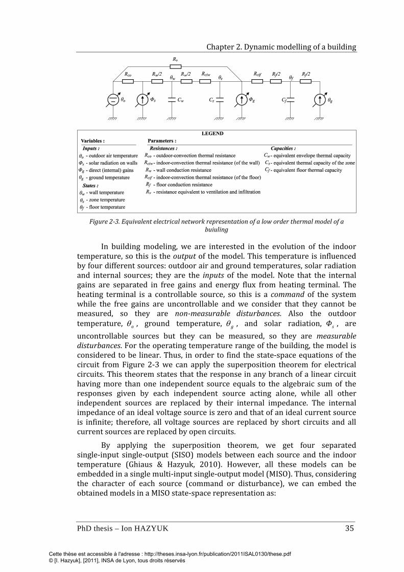
Chapter 2. Dynamic modelling of a building
PhD thesis – Ion HAZYUK 35
Figure 2-3. Equivalent electrical network representation of a low order thermal model of a
buiuling
In building modeling, we are interested in the evolution of the indoor temperature, so this is the output of the model. This temperature is influenced by four different sources: outdoor air and ground temperatures, solar radiation and internal sources; they are the inputs of the model. Note that the internal gains are separated in free gains and energy flux from heating terminal. The heating terminal is a controllable source, so this is a command of the system while the free gains are uncontrollable and we consider that they cannot be measured, so they are non-measurable disturbances. Also the outdoor temperature, oθ , ground temperature, gθ , and solar radiation, sΦ , are uncontrollable sources but they can be measured, so they are measurable disturbances. For the operating temperature range of the building, the model is considered to be linear. Thus, in order to find the state-space equations of the circuit from Figure 2-3 we can apply the superposition theorem for electrical circuits. This theorem states that the response in any branch of a linear circuit having more than one independent source equals to the algebraic sum of the responses given by each independent source acting alone, while all other independent sources are replaced by their internal impedance. The internal impedance of an ideal voltage source is zero and that of an ideal current source is infinite; therefore, all voltage sources are replaced by short circuits and all current sources are replaced by open circuits.
By applying the superposition theorem, we get four separated single-input single-output (SISO) models between each source and the indoor temperature (Ghiaus & Hazyuk, 2010). However, all these models can be embedded in a single multi-input single-output model (MISO). Thus, considering the character of each source (command or disturbance), we can embed the obtained models in a MISO state-space representation as:
Cette thèse est accessible à l'adresse : http://theses.insa-lyon.fr/publication/2011ISAL0130/these.pdf © [I. Hazyuk], [2011], INSA de Lyon, tous droits réservés
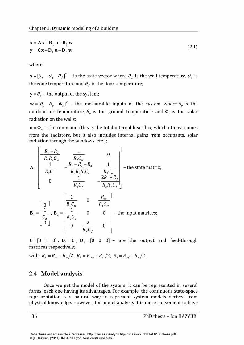
Chapter 2. Dynamic modeling of a building
36 PhD thesis – Ion HAZYUK
wDuDxCywBuBxAx
21
21
++=++=
(2.1)
where:
Tfzw ][ θθθ=x – is the state vector where wθ is the wall temperature, zθ is
the zone temperature and fθ is the floor temperature;
zθ=y – the output of the system; T
sgo Φ ][ θθ=w – the measurable inputs of the system where oθ is the outdoor air temperature, gθ is the ground temperature and sΦ is the solar radiation on the walls;
gΦ=u – the command (this is the total internal heat flux, which utmost comes from the radiators, but it also includes internal gains from occupants, solar radiation through the windows, etc.);
+−
++−
+−
=
ff
f
f
aav
v
a
ww
CRRRR
CR
CRCRRRRRR
CR
CRCRRRR
3
3
3
332
32
2
221
21
210
11
01
A – the state matrix;
=
0
10
1aC
B ,
=
020
001
0111
2
ff
av
w
co
w
CR
CR
CRR
CR
B – the input matrices;
]010[=C , 01 =D , ]000[2 =D – are the output and feed-through matrices respectively;
with: 21 wco RRR += , 22 wciw RRR += , 23 fcif RRR += .
2.4 Model analysis
Once we get the model of the system, it can be represented in several forms, each one having its advantages. For example, the continuous state-space representation is a natural way to represent system models derived from physical knowledge. However, for model analysis it is more convenient to have
Cette thèse est accessible à l'adresse : http://theses.insa-lyon.fr/publication/2011ISAL0130/these.pdf © [I. Hazyuk], [2011], INSA de Lyon, tous droits réservés
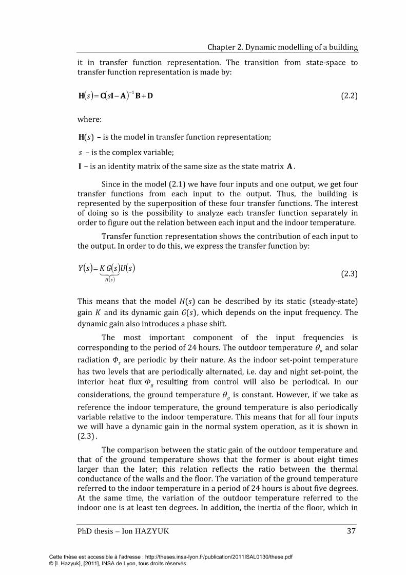
Chapter 2. Dynamic modelling of a building
PhD thesis – Ion HAZYUK 37
it in transfer function representation. The transition from state-space to transfer function representation is made by:
( ) ( ) DBAICH +−= −1ss (2.2)
where:
)(sH – is the model in transfer function representation;
s – is the complex variable;
I – is an identity matrix of the same size as the state matrix A .
Since in the model (2.1) we have four inputs and one output, we get four transfer functions from each input to the output. Thus, the building is represented by the superposition of these four transfer functions. The interest of doing so is the possibility to analyze each transfer function separately in order to figure out the relation between each input and the indoor temperature.
Transfer function representation shows the contribution of each input to the output. In order to do this, we express the transfer function by:
( ) ( )( )
( )sUsGKsYsH
= (2.3)
This means that the model )(sH can be described by its static (steady-state) gain K and its dynamic gain )(sG , which depends on the input frequency. The dynamic gain also introduces a phase shift.
The most important component of the input frequencies is corresponding to the period of 24 hours. The outdoor temperature oθ and solar radiation sΦ are periodic by their nature. As the indoor set-point temperature has two levels that are periodically alternated, i.e. day and night set-point, the interior heat flux gΦ resulting from control will also be periodical. In our considerations, the ground temperature gθ is constant. However, if we take as reference the indoor temperature, the ground temperature is also periodically variable relative to the indoor temperature. This means that for all four inputs we will have a dynamic gain in the normal system operation, as it is shown in (2.3) .
The comparison between the static gain of the outdoor temperature and that of the ground temperature shows that the former is about eight times larger than the later; this relation reflects the ratio between the thermal conductance of the walls and the floor. The variation of the ground temperature referred to the indoor temperature in a period of 24 hours is about five degrees. At the same time, the variation of the outdoor temperature referred to the indoor one is at least ten degrees. In addition, the inertia of the floor, which in
Cette thèse est accessible à l'adresse : http://theses.insa-lyon.fr/publication/2011ISAL0130/these.pdf © [I. Hazyuk], [2011], INSA de Lyon, tous droits réservés
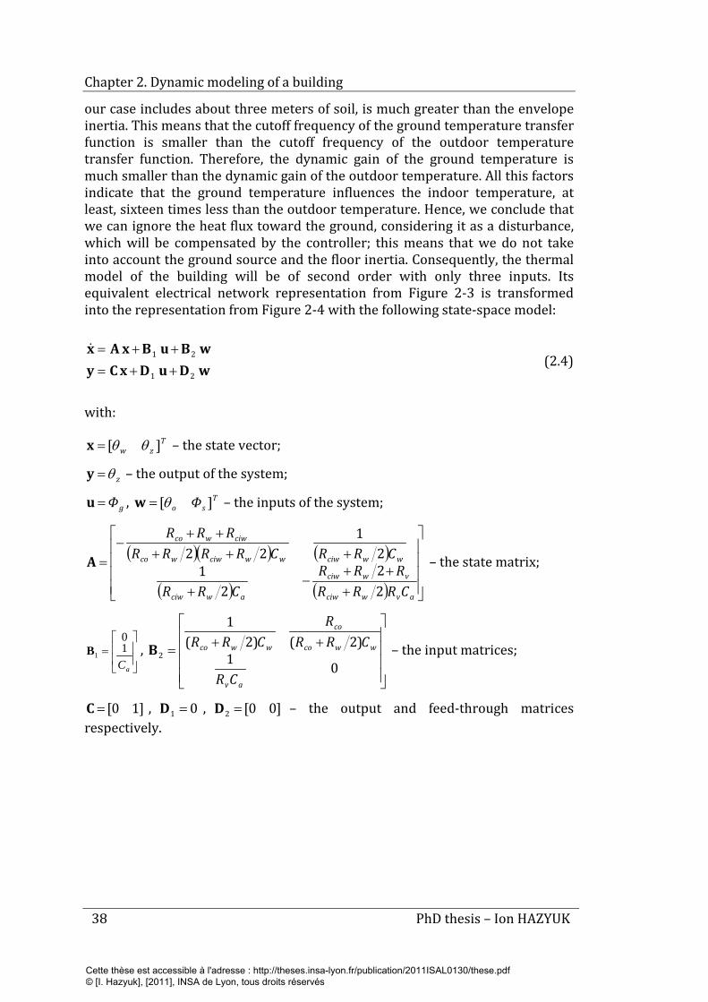
Chapter 2. Dynamic modeling of a building
38 PhD thesis – Ion HAZYUK
our case includes about three meters of soil, is much greater than the envelope inertia. This means that the cutoff frequency of the ground temperature transfer function is smaller than the cutoff frequency of the outdoor temperature transfer function. Therefore, the dynamic gain of the ground temperature is much smaller than the dynamic gain of the outdoor temperature. All this factors indicate that the ground temperature influences the indoor temperature, at least, sixteen times less than the outdoor temperature. Hence, we conclude that we can ignore the heat flux toward the ground, considering it as a disturbance, which will be compensated by the controller; this means that we do not take into account the ground source and the floor inertia. Consequently, the thermal model of the building will be of second order with only three inputs. Its equivalent electrical network representation from Figure 2-3 is transformed into the representation from Figure 2-4 with the following state-space model:
wDuDxCywBuBxAx
21
21
++=++=
(2.4)
with:
Tzw ][ θθ=x – the state vector;
zθ=y – the output of the system;
gΦ=u , Tso Φ ][θ=w – the inputs of the system;
( )( ) ( )
( ) ( )
+++
−+
+++++
−=
avwciw
vwciw
awciw
wwciwwwciwwco
ciwwco
CRRRRRR
CRR
CRRCRRRRRRR
22
21
21
22A – the state matrix;
=
aC10
1B ,
++=
01)2()2(
1
2
av
wwco
co
wwco
CR
CRRR
CRRB – the input matrices;
]10[=C , 01 =D , ]00[2 =D – the output and feed-through matrices respectively.
Cette thèse est accessible à l'adresse : http://theses.insa-lyon.fr/publication/2011ISAL0130/these.pdf © [I. Hazyuk], [2011], INSA de Lyon, tous droits réservés
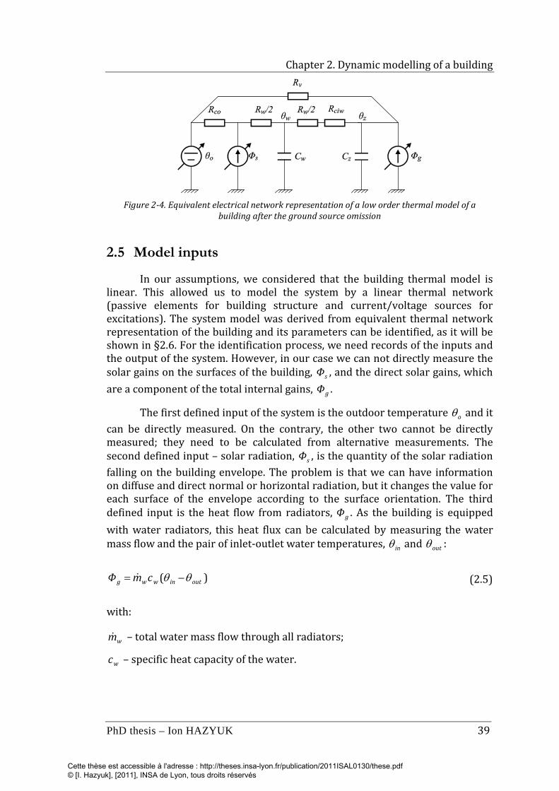
Chapter 2. Dynamic modelling of a building
PhD thesis – Ion HAZYUK 39
Figure 2-4. Equivalent electrical network representation of a low order thermal model of a
building after the ground source omission
2.5 Model inputs
In our assumptions, we considered that the building thermal model is linear. This allowed us to model the system by a linear thermal network (passive elements for building structure and current/voltage sources for excitations). The system model was derived from equivalent thermal network representation of the building and its parameters can be identified, as it will be shown in §2.6. For the identification process, we need records of the inputs and the output of the system. However, in our case we can not directly measure the solar gains on the surfaces of the building, sΦ , and the direct solar gains, which are a component of the total internal gains, gΦ .
The first defined input of the system is the outdoor temperature oθ and it can be directly measured. On the contrary, the other two cannot be directly measured; they need to be calculated from alternative measurements. The second defined input – solar radiation, sΦ , is the quantity of the solar radiation falling on the building envelope. The problem is that we can have information on diffuse and direct normal or horizontal radiation, but it changes the value for each surface of the envelope according to the surface orientation. The third defined input is the heat flow from radiators, gΦ . As the building is equipped with water radiators, this heat flux can be calculated by measuring the water mass flow and the pair of inlet-outlet water temperatures, inθ and outθ :
)( outinwwg cmΦ θθ −= (2.5)
with:
wm – total water mass flow through all radiators;
wc – specific heat capacity of the water.
Cette thèse est accessible à l'adresse : http://theses.insa-lyon.fr/publication/2011ISAL0130/these.pdf © [I. Hazyuk], [2011], INSA de Lyon, tous droits réservés
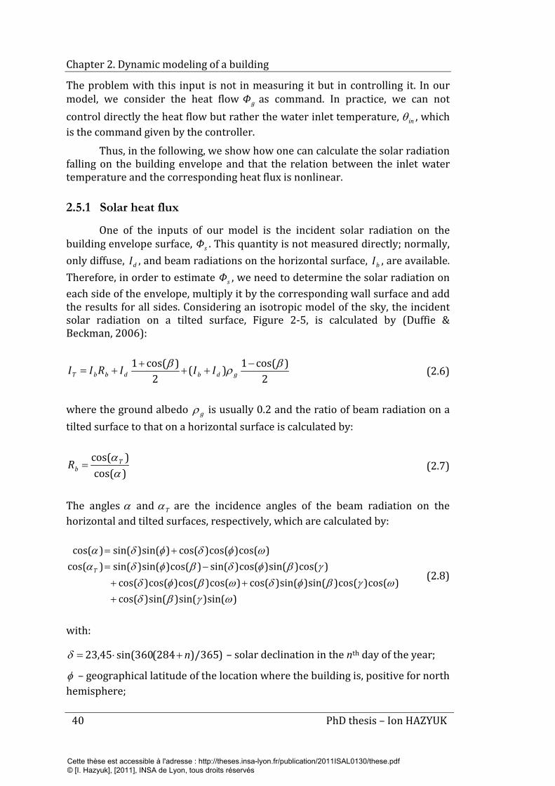
Chapter 2. Dynamic modeling of a building
40 PhD thesis – Ion HAZYUK
The problem with this input is not in measuring it but in controlling it. In our model, we consider the heat flow gΦ as command. In practice, we can not control directly the heat flow but rather the water inlet temperature, inθ , which is the command given by the controller.
Thus, in the following, we show how one can calculate the solar radiation falling on the building envelope and that the relation between the inlet water temperature and the corresponding heat flux is nonlinear.
2.5.1 Solar heat flux
One of the inputs of our model is the incident solar radiation on the building envelope surface, sΦ . This quantity is not measured directly; normally, only diffuse, dI , and beam radiations on the horizontal surface, bI , are available. Therefore, in order to estimate sΦ , we need to determine the solar radiation on each side of the envelope, multiply it by the corresponding wall surface and add the results for all sides. Considering an isotropic model of the sky, the incident solar radiation on a tilted surface, Figure 2-5, is calculated by (Duffie & Beckman, 2006):
2)cos(1)(
2)cos(1 βρβ −
+++
+= gdbdbbT IIIRII (2.6)
where the ground albedo gρ is usually 0.2 and the ratio of beam radiation on a tilted surface to that on a horizontal surface is calculated by:
)cos()cos(
ααT
bR = (2.7)
The angles α and Tα are the incidence angles of the beam radiation on the horizontal and tilted surfaces, respectively, which are calculated by:
)sin()sin()sin()cos()cos()cos()sin()sin()cos()cos()cos()cos()cos(
)cos()sin()cos()sin()cos()sin()sin()cos()cos()cos()cos()sin()sin()cos(
ωγβδωγβφδωβφδ
γβφδβφδαωφδφδα
+++
−=+=
T (2.8)
with:
)365/)284(360sin(45,23 n+⋅=δ – solar declination in the nth day of the year;
φ – geographical latitude of the location where the building is, positive for north hemisphere;
Cette thèse est accessible à l'adresse : http://theses.insa-lyon.fr/publication/2011ISAL0130/these.pdf © [I. Hazyuk], [2011], INSA de Lyon, tous droits réservés
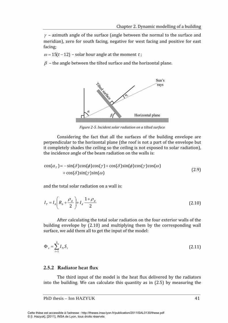
Chapter 2. Dynamic modelling of a building
PhD thesis – Ion HAZYUK 41
γ – azimuth angle of the surface (angle between the normal to the surface and meridian), zero for south facing, negative for west facing and positive for east facing;
)12(15 −= tω – solar hour angle at the moment t ;
β – the angle between the tilted surface and the horizontal plane.
Figure 2-5. Incident solar radiation on a tilted surface
Considering the fact that all the surfaces of the building envelope are perpendicular to the horizontal plane (the roof is not a part of the envelope but it completely shades the ceiling so the ceiling is not exposed to solar radiation), the incidence angle of the beam radiation on the walls is:
)sin()sin()cos()cos()cos()sin()cos()cos()cos()sin()cos(
ωγδωγφδγφδα
++−=T (2.9)
and the total solar radiation on a wall is:
21
2g
dg
bbT IRIIρρ +
+
+= (2.10)
After calculating the total solar radiation on the four exterior walls of the building envelope by (2.10) and multiplying them by the corresponding wall surface, we add them all to get the input of the model:
∑=
=Φ4
1iiTis SI (2.11)
2.5.2 Radiator heat flux
The third input of the model is the heat flux delivered by the radiators into the building. We can calculate this quantity as in (2.5) by measuring the
Cette thèse est accessible à l'adresse : http://theses.insa-lyon.fr/publication/2011ISAL0130/these.pdf © [I. Hazyuk], [2011], INSA de Lyon, tous droits réservés
Chapter 2. Dynamic modeling of a building
42 PhD thesis – Ion HAZYUK
inlet and outlet water temperatures. However, if we determine the model between the indoor air temperature, zθ , and the heat flux, gΦ , we could not use it for control because we cannot control directly the heat flux. This energy flow depends on several parameters like indoor air temperature, mean radiator temperature, interior walls surface temperature and water mass flow through radiators. In practice, we can control only the water inlet temperature or the water flow; acting on water flow may induce hydraulic instabilities. Thus, the question that naturally arises is why not to determine a model between the indoor air temperature and the inlet water temperature. Here we give an explanation why it is preferable not to do so and how to overcome this problem.
The thermal energy coming from the radiators, gΦ , is transmitted to the indoor environment via convection and radiation. Generally, the ratio between these two is considered to be 50 %, although it may vary depending on many factors. The heat transferred through convection depends on the difference between the mean radiator temperature and indoor air temperature while the heat transferred through radiation depends on the difference between the mean radiator temperature and the temperature of the surfaces inside the building. However, all the indoor surfaces except the interior surfaces of the envelope are part of the internal mass. Therefore, for simplicity we will consider that the radiative heat transfer depends on the difference between the radiators surface temperature and the indoor heat capacity temperature.
In most papers, the radiative heat transfer is neglected or it is approximated by a linear law (Liao & Dexter, 2004). If the difference between the temperatures of the surfaces is not too large, the radiative heat flux density transferred from a hot surface to the colder one is calculated by:
)( 44coldhotr TT −= εσϕ (2.12)
where:
ε – surface emissivity;
σ – Stefan-Boltzmann constant;
T – surface temperature in Kelvin degrees.
The relation (2.12) can also be represented in the following form:
)())(( 22coldhot
h
coldhotcoldhotr TTTTTTr
−++=
εσϕ (2.13)
The linearization of this relation is based on the following consideration: in the building, the hot surface is always the radiator and its temperature varies between 20 and 60 °C. The cold surfaces are all the surfaces inside the building and their temperature varies roughly between 15 and 20 °C. As in relation (2.13) the temperature is represented on the absolute scale,
Cette thèse est accessible à l'adresse : http://theses.insa-lyon.fr/publication/2011ISAL0130/these.pdf © [I. Hazyuk], [2011], INSA de Lyon, tous droits réservés
Chapter 2. Dynamic modelling of a building
PhD thesis – Ion HAZYUK 43
][273][ CKT surface °+= θ , the usual temperature variations in the building are relatively small compared to their absolute value. Therefore they do not have a significant impact on the first two parentheses, which are approximated by a constant heat transfer coefficient, rh , by taking the mean temperature of the surfaces.
Concerning the convective heat transfer, the heat flux density for a vertical surface, taller than 30 cm is described by the following law (Incropera, et al., 2006) :
( ) ( )airsurf
h
airsurfc TTTTc
−−= 4178.1
ϕ (2.14)
Here also the first parenthesis is considered to be approximately constant so together with its coefficient they form the convective heat transfer coefficient, ch . Thus, making the hypothesis that the radiative and convective heat transfer coefficients are constant, the total heat flux density is obtained by adding relations (2.13) and (2.14) so we get the following linear law:
( )( )coldhot
h
rcrcT TThhT
−+=+=
ϕϕϕ (2.15)
The total heat flux delivered by the radiator is obtained by multiplying the total heat flux density, Tϕ , by the radiators surface radS :
Tradg SΦ ϕ= (2.16)
The problem is that the temperature difference between the radiators and the thermal mass varies usually between zero and forty to fifty degrees. This variation is large enough in order to violate the hypothesis that the total heat transfer coefficient, Th , is constant on the entire operating temperature range. By using a simulation software (Husaunndee, Lahrech, Vaezi-Nejad & Visier, 1997), we varied the inlet water temperature of radiators and recorded the indoor mean temperature, zθ , and the heat flux delivered by the radiators using the relation (2.5). As expected, we obtained a nonlinear dependence between the heat flux delivered by the radiators and the temperature difference between inlet water and mean zone temperature, Figure 2-6 (a). The nonlinearity is better illustrated in Figure 2-6 (b) where the total conductance is:
zin
gTrad
ΦhS
θθ −= (2.17)
Cette thèse est accessible à l'adresse : http://theses.insa-lyon.fr/publication/2011ISAL0130/these.pdf © [I. Hazyuk], [2011], INSA de Lyon, tous droits réservés
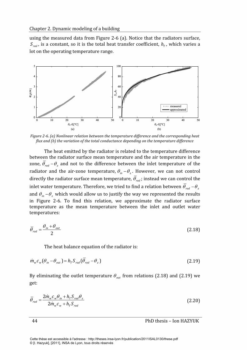
Chapter 2. Dynamic modeling of a building
44 PhD thesis – Ion HAZYUK
using the measured data from Figure 2-6 (a). Notice that the radiators surface, radS , is a constant, so it is the total heat transfer coefficient, Th , which varies a
lot on the operating temperature range.
Figure 2-6. (a) Nonlinear relation between the temperature difference and the corresponding heat
flux and (b) the variation of the total conductance depending on the temperature difference
The heat emitted by the radiator is related to the temperature difference between the radiator surface mean temperature and the air temperature in the zone, zrad θθ − and not to the difference between the inlet temperature of the radiator and the air-zone temperature, zin θθ − . However, we can not control directly the radiator surface mean temperature, radθ ; instead we can control the inlet water temperature. Therefore, we tried to find a relation between zrad θθ − and zin θθ − which would allow us to justify the way we represented the results in Figure 2-6. To find this relation, we approximate the radiator surface temperature as the mean temperature between the inlet and outlet water temperatures:
2outin
radθθ
θ+
= (2.18)
The heat balance equation of the radiator is:
)()( zradradToutinww Shcm θθθθ −=− (2.19)
By eliminating the outlet temperature outθ from relations (2.18) and (2.19) we get:
radTww
zradTinwwrad Shcm
Shcm++
=
22 θθ
θ (2.20)
Cette thèse est accessible à l'adresse : http://theses.insa-lyon.fr/publication/2011ISAL0130/these.pdf © [I. Hazyuk], [2011], INSA de Lyon, tous droits réservés
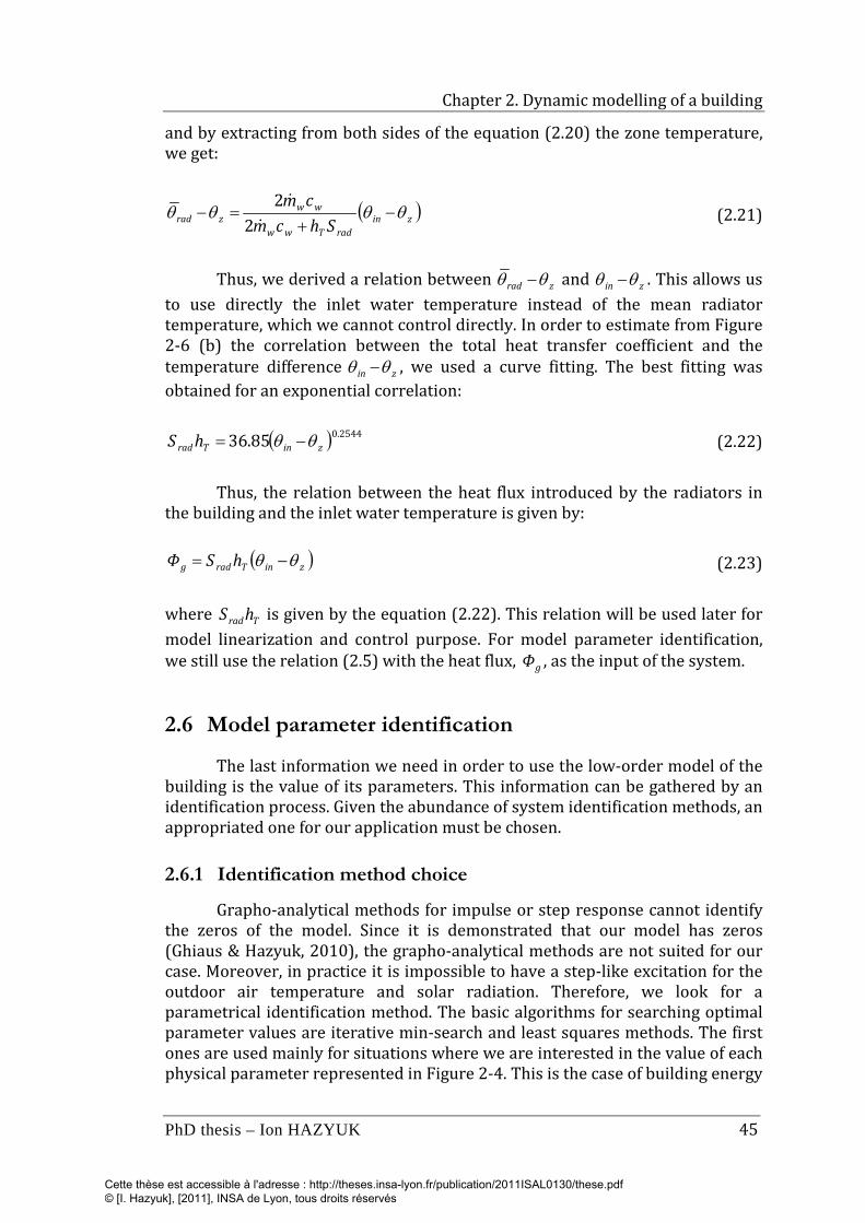
Chapter 2. Dynamic modelling of a building
PhD thesis – Ion HAZYUK 45
and by extracting from both sides of the equation (2.20) the zone temperature, we get:
( )zinradTww
wwzrad Shcm
cmθθθθ −
+=−
22
(2.21)
Thus, we derived a relation between zrad θθ − and zin θθ − . This allows us to use directly the inlet water temperature instead of the mean radiator temperature, which we cannot control directly. In order to estimate from Figure 2-6 (b) the correlation between the total heat transfer coefficient and the temperature difference zin θθ − , we used a curve fitting. The best fitting was obtained for an exponential correlation:
( ) 2544.085.36 zinTrad hS θθ −= (2.22)
Thus, the relation between the heat flux introduced by the radiators in the building and the inlet water temperature is given by:
( )zinTradg hSΦ θθ −= (2.23)
where TradhS is given by the equation (2.22). This relation will be used later for model linearization and control purpose. For model parameter identification, we still use the relation (2.5) with the heat flux, gΦ , as the input of the system.
2.6 Model parameter identification
The last information we need in order to use the low-order model of the building is the value of its parameters. This information can be gathered by an identification process. Given the abundance of system identification methods, an appropriated one for our application must be chosen.
2.6.1 Identification method choice
Grapho-analytical methods for impulse or step response cannot identify the zeros of the model. Since it is demonstrated that our model has zeros (Ghiaus & Hazyuk, 2010), the grapho-analytical methods are not suited for our case. Moreover, in practice it is impossible to have a step-like excitation for the outdoor air temperature and solar radiation. Therefore, we look for a parametrical identification method. The basic algorithms for searching optimal parameter values are iterative min-search and least squares methods. The first ones are used mainly for situations where we are interested in the value of each physical parameter represented in Figure 2-4. This is the case of building energy
Cette thèse est accessible à l'adresse : http://theses.insa-lyon.fr/publication/2011ISAL0130/these.pdf © [I. Hazyuk], [2011], INSA de Lyon, tous droits réservés
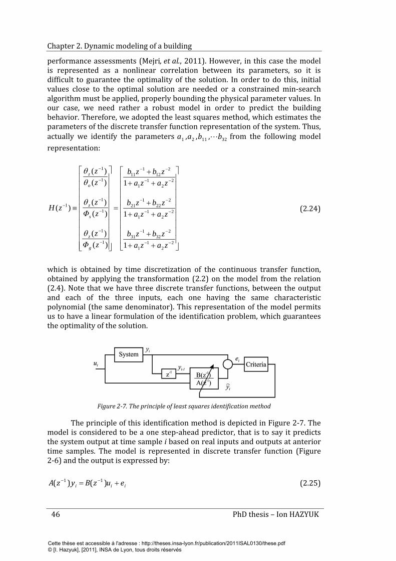
Chapter 2. Dynamic modeling of a building
46 PhD thesis – Ion HAZYUK
performance assessments (Mejri, et al., 2011). However, in this case the model is represented as a nonlinear correlation between its parameters, so it is difficult to guarantee the optimality of the solution. In order to do this, initial values close to the optimal solution are needed or a constrained min-search algorithm must be applied, properly bounding the physical parameter values. In our case, we need rather a robust model in order to predict the building behavior. Therefore, we adopted the least squares method, which estimates the parameters of the discrete transfer function representation of the system. Thus, actually we identify the parameters 321121 ,,, bbaa from the following model representation:
+++
+++
+++
=
≡
−−
−−
−−
−−
−−
−−
−
−
−
−
−
−
−
22
11
232
131
22
11
222
121
22
11
212
111
1
1
1
1
1
1
1
1
1
1
)()(
)()(
)()(
)(
zazazbzb
zazazbzb
zazazbzb
zΦz
zΦz
zz
zH
g
z
s
z
o
z
θ
θ
θθ
(2.24)
which is obtained by time discretization of the continuous transfer function, obtained by applying the transformation (2.2) on the model from the relation (2.4). Note that we have three discrete transfer functions, between the output and each of the three inputs, each one having the same characteristic polynomial (the same denominator). This representation of the model permits us to have a linear formulation of the identification problem, which guarantees the optimality of the solution.
Figure 2-7. The principle of least squares identification method
The principle of this identification method is depicted in Figure 2-7. The model is considered to be a one step-ahead predictor, that is to say it predicts the system output at time sample i based on real inputs and outputs at anterior time samples. The model is represented in discrete transfer function (Figure 2-6) and the output is expressed by:
iii euzByzA += −− )()( 11 (2.25)
Cette thèse est accessible à l'adresse : http://theses.insa-lyon.fr/publication/2011ISAL0130/these.pdf © [I. Hazyuk], [2011], INSA de Lyon, tous droits réservés
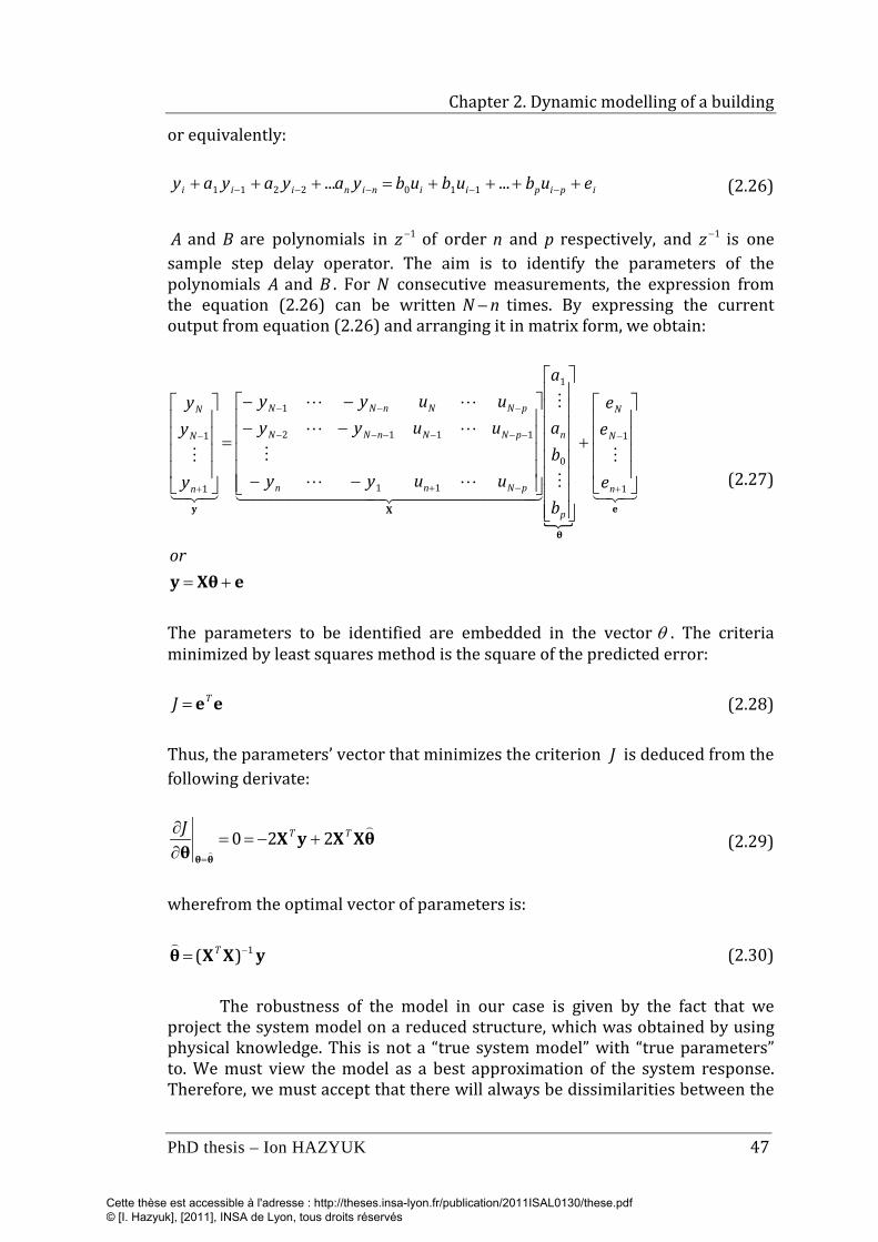
Chapter 2. Dynamic modelling of a building
PhD thesis – Ion HAZYUK 47
or equivalently:
ipipiininiii eubububyayayay ++++=+++ −−−−− ...... 1102211 (2.26)
A and B are polynomials in 1−z of order n and p respectively, and 1−z is one sample step delay operator. The aim is to identify the parameters of the polynomials A and B . For N consecutive measurements, the expression from the equation (2.26) can be written nN − times. By expressing the current output from equation (2.26) and arranging it in matrix form, we obtain:
eXθy
e
θ
Xy
+=
+
−−
−−−−
=
+
−
−+
−−−−−−
−−−
+
−
or
e
ee
b
ba
a
uuyy
uuyyuuyy
y
yy
n
N
N
p
n
pNnn
pNNnNN
pNNnNN
n
N
N
1
1
0
1
11
1112
1
1
1
(2.27)
The parameters to be identified are embedded in the vector θ . The criteria minimized by least squares method is the square of the predicted error:
eeTJ = (2.28)
Thus, the parameters’ vector that minimizes the criterion J is deduced from the following derivate:
θXXyXθ θθ
TTJ 220 +−==∂∂
=
(2.29)
wherefrom the optimal vector of parameters is:
yXXθ 1)( −= T
(2.30)
The robustness of the model in our case is given by the fact that we project the system model on a reduced structure, which was obtained by using physical knowledge. This is not a “true system model” with “true parameters” to. We must view the model as a best approximation of the system response. Therefore, we must accept that there will always be dissimilarities between the
Cette thèse est accessible à l'adresse : http://theses.insa-lyon.fr/publication/2011ISAL0130/these.pdf © [I. Hazyuk], [2011], INSA de Lyon, tous droits réservés

Chapter 2. Dynamic modeling of a building
48 PhD thesis – Ion HAZYUK
model and the building response. If we searched to reduce this error by varying the model parameters and the system structure, we would risk over fitting: we get a good similarity between the model and system response in the identification process, but when we test the identified model on a different excitation signal, we get important differences between the responses. On the contrary, the physical phenomena will not change when the excitations are varying in the operating range. Thus, by remaining in the framework of this imposed structure, we have the certainty of identifying a robust system model. This is the motivation to have the structure of the model derived from basic physical knowledge.
2.6.2 Parameter identification
For the model parameters identification, we must record the inputs and the output of the system, and, then, apply the chosen identification method. The question is which kind of input signals must be applied to find good quality parameters. In practice, we are very limited in this choice because the circumstances do not allow all types of inputs. First, we cannot act in any way on the outdoor temperature and solar radiation. Then, even for the internal heat flux, we are limited in imposing a form to the input because usually the building is inhabited and we can not move beyond the accepted comfort norms. On the other hand, it costs enormous to test an uninhabited building. As the parameter identification on a real building is difficult, an alternative is to identify the parameters of a low order model that fits the white-box model of the building. In simulation, we can apply any input signal as well as other handy manipulations. Therefore we make the identification using data records obtained from simulation of the reference building.
Before starting the identification, several theoretical details must be recalled. First, we have to choose the adequate excitation signal. Its role is to excite the system modes. Even if we are in simulation, we have not imposed an atypical form for the outdoor temperature and solar radiation; we used the statistical whether records offered by the simulation program. On the contrary, for the internal heat flux, we act on the inlet water temperature and we imposed a pseudo-random binary sequence (PRBS). This sequence must be long enough in order to generate the frequencies which would excite even the most inert modes of the system.
Secondly, when we start the identification of a model in transfer function representation, the system must be in initial zero conditions. In our case, the system states are the zone and wall temperatures, it means that they all must be zero. In practice, it is impossible to guarantee this condition; assuring initial zero conditions is another benefit of using white-box simulation model. We switched the inlet water temperature between 20 and 60 °C according to a PRBS for a period of four months. Standard weather records for December, January, February and March in Lyon, France, were used for outdoor temperature and solar radiation. With these inputs, we simulated the reference building for a period of four months with a sampling time of one minute. We computed the
Cette thèse est accessible à l'adresse : http://theses.insa-lyon.fr/publication/2011ISAL0130/these.pdf © [I. Hazyuk], [2011], INSA de Lyon, tous droits réservés
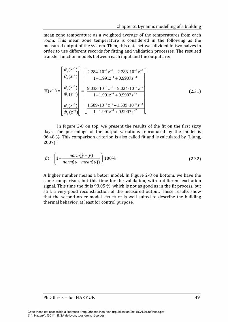
Chapter 2. Dynamic modelling of a building
PhD thesis – Ion HAZYUK 49
mean zone temperature as a weighted average of the temperatures from each room. This mean zone temperature is considered in the following as the measured output of the system. Then, this data set was divided in two halves in order to use different records for fitting and validation processes. The resulted transfer function models between each input and the output are:
+−⋅−⋅
+−⋅−⋅
+−⋅−⋅
=
≡
−−
−−−−
−−
−−−−
−−
−−−−
−
−
−
−
−
−
−
21
2515
21
2717
21
2313
1
1
1
1
1
1
1
9907.0991.1110589.110589.1
9907.0991.1110024.910033.9
9907.0991.1110283.210284.2
)()(
)()(
)()(
)(
zzzz
zzzz
zzzz
zΦz
zΦz
zz
z
g
z
s
z
o
z
θ
θ
θθ
H (2.31)
In Figure 2-8 on top, we present the results of the fit on the first sixty days. The percentage of the output variations reproduced by the model is 96.48 %. This comparison criterion is also called fit and is calculated by (Ljung, 2007):
%100))((
)ˆ(1 ⋅
−
−−=
ymeanynormyynormfit (2.32)
A higher number means a better model. In Figure 2-8 on bottom, we have the same comparison, but this time for the validation, with a different excitation signal. This time the fit is 93.05 %, which is not as good as in the fit process, but still, a very good reconstruction of the measured output. These results show that the second order model structure is well suited to describe the building thermal behavior, at least for control purpose.
Cette thèse est accessible à l'adresse : http://theses.insa-lyon.fr/publication/2011ISAL0130/these.pdf © [I. Hazyuk], [2011], INSA de Lyon, tous droits réservés
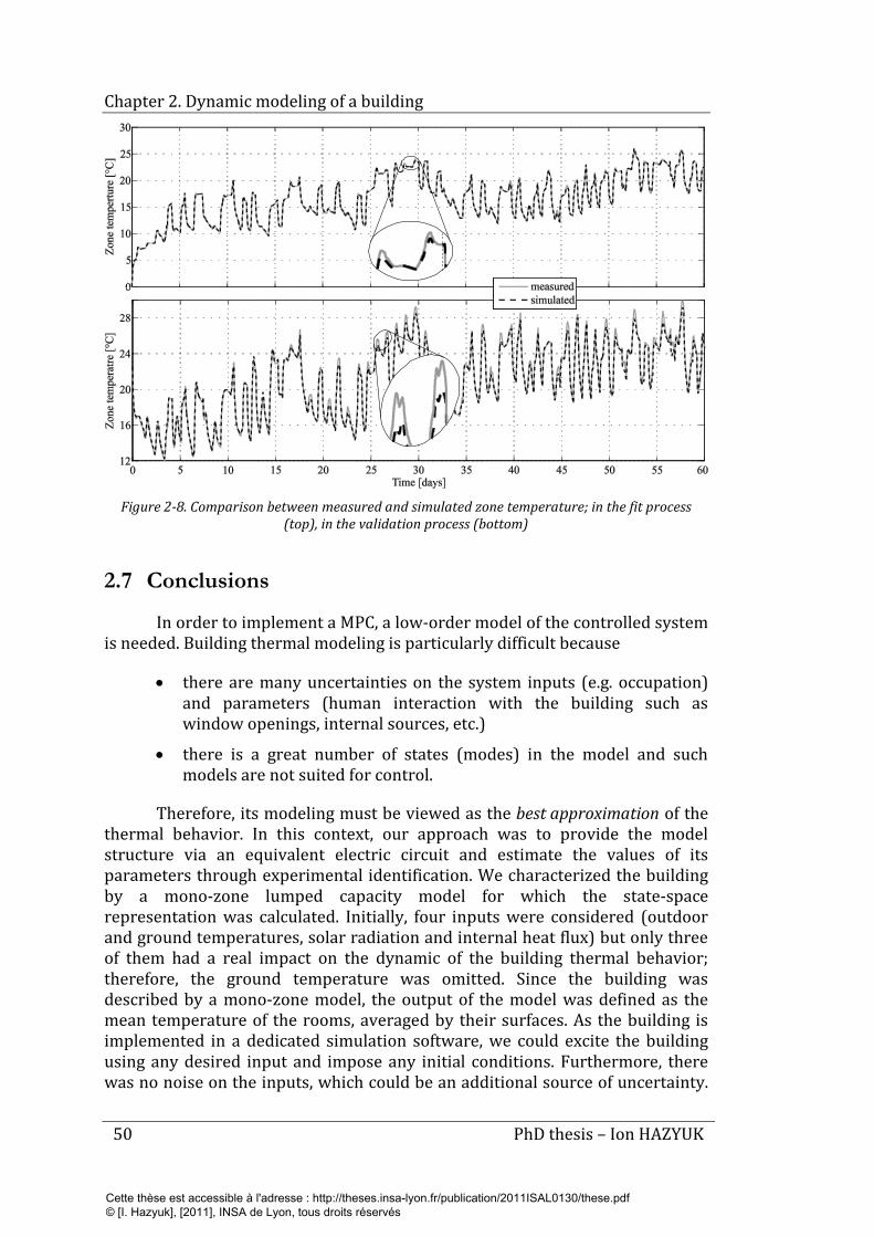
Chapter 2. Dynamic modeling of a building
50 PhD thesis – Ion HAZYUK
Figure 2-8. Comparison between measured and simulated zone temperature; in the fit process
(top), in the validation process (bottom)
2.7 Conclusions
In order to implement a MPC, a low-order model of the controlled system is needed. Building thermal modeling is particularly difficult because
• there are many uncertainties on the system inputs (e.g. occupation) and parameters (human interaction with the building such as window openings, internal sources, etc.)
• there is a great number of states (modes) in the model and such models are not suited for control.
Therefore, its modeling must be viewed as the best approximation of the thermal behavior. In this context, our approach was to provide the model structure via an equivalent electric circuit and estimate the values of its parameters through experimental identification. We characterized the building by a mono-zone lumped capacity model for which the state-space representation was calculated. Initially, four inputs were considered (outdoor and ground temperatures, solar radiation and internal heat flux) but only three of them had a real impact on the dynamic of the building thermal behavior; therefore, the ground temperature was omitted. Since the building was described by a mono-zone model, the output of the model was defined as the mean temperature of the rooms, averaged by their surfaces. As the building is implemented in a dedicated simulation software, we could excite the building using any desired input and impose any initial conditions. Furthermore, there was no noise on the inputs, which could be an additional source of uncertainty.
Cette thèse est accessible à l'adresse : http://theses.insa-lyon.fr/publication/2011ISAL0130/these.pdf © [I. Hazyuk], [2011], INSA de Lyon, tous droits réservés
Chapter 2. Dynamic modelling of a building
PhD thesis – Ion HAZYUK 51
This allowed us to use the standard least squares method for parameter identification. Even in these circumstances, we tried to get closer to reality: we excited the building using real solar radiation and outdoor temperature, whose data was gathered from statistical meteorological records. For the third input, we used the heat flux resulted by switching the radiators inlet water temperature between 20 and 60 °C, according to a pseudorandom binary signal. The simulation was carried out for a four months period and the results were divided in two parts. The first data sequence was used for parameter identification and the second one for model validation.
As the handled input is the inlet water temperature and not the heat flux delivered by the radiators, we figured out that the relation between these two is nonlinear. Therefore, we showed how this correlation could be expressed and identified in order to be used for model linearization and control.
The model structure was obtained in continuous state-space representation. However, the identification using least squares method requires a model structure in discrete transfer function representation. Therefore, we determined the discrete transfer-function structure that is equivalent to the continuous state-space structure, which in our case gave a two poles – one zero model structure. The model validation showed that the identified model can reproduce the building thermal behavior with a good fidelity (the fit between the results larger than 90 %).
Nevertheless, building model parameter identification is far to be a solved problem. Even if the theoretical tools are very advanced, their practical application for buildings is still not well handled. It is not acceptable to excite the building as we need while it is occupied and an experimental campaign of an unoccupied building is expensive. Thus, the research in this direction could bring out some real contributions, not only to MPC but generally for all model based control strategies.
Cette thèse est accessible à l'adresse : http://theses.insa-lyon.fr/publication/2011ISAL0130/these.pdf © [I. Hazyuk], [2011], INSA de Lyon, tous droits réservés
Chapter 2. Dynamic modeling of a building
52 PhD thesis – Ion HAZYUK
References
Achterbosch, G. G. J., de Jong, P. P. G., Krist-Spit, C. E., van der Meulen, S. F. & Verberne, J. (1985). The development of a comvenient thermal dynamic building model. Energy and Buildings, 8(3), 183-196.
Bénard, C., Guerrier, B. & Rosset-Louërat, M.-M. (1992). Optimal Building Energy Management: Part I---Modeling. Journal of Solar Energy Engineering, 114, 2-12.
Boaventura Cunha, J., Couto, C. & Ruano, A. E. (1997). Real-time parameter estimation of dynamic temperature models for greenhouse environmental control. Control Engineering Practice, 5(10), 1473-1481.
Chen, T. Y. & Athienitis, A. K. (2003). Investigation of practical issues in building thermal parameter estimation. Building and Environment, 38(8), 1027-1038.
Clarke, J. A. (2001). Energy Simulation in Building Design (2nd ed.). Oxford: Butterworth-Heinemann.
Coley, D. A. & Penman, J. M. (1996). Simplified thermal response modelling in building energy management. Paper III: Demonstration of a working controller. Building and Environment, 31(2), 93-97.
Duffie, J. A. & Beckman, W. A. (2006). Solar Engineering of Thermal Processes (3rd ed.). Hoboken, NJ: John Wiley & Sons.
EnergyPlus (2009). EnergyPlus Engineering Reference: The Reference to EnergyPlus Calculations: Lawrence Berkeley National Laboratory.
García-Sanz, M. (1997). A reduced model of central heating systems as a realistic scenario for analyzing control strategies. Applied Mathematical Modelling, 21(9), 535-545.
Ghiaus, C., Chicinas, A. & Inard, C. (2007). Grey-box identification of air-handling unit elements. Control Engineering Practice, 15(4), 421-433.
Ghiaus, C. & Hazyuk, I. (2010). Calculation of optimal thermal load of intermittently heated buildings. Energy and Buildings, 42(8), 1248-1258.
Gouda, M. M., Danaher, S. & Underwood, C. P. (2002). Building thermal model reduction using nonlinear constrained optimization. Building and Environment, 37(12), 1255-1265.
Husaunndee, A., Lahrech, R., Vaezi-Nejad, H. & Visier, J. C. (1997). SIMBAD: A simulation toolbox for the design and test of HVAC control systems. In: 5th international IBPSA conference, September 8-10, 1997, Prague, Czech Republic.
Incropera, F. P., DeWitt, D. P., Bergman, T. L. & Lavine, A. S. (2006). Fundamentals of Heat and Mass Transfer (6th ed.): John Wiley & Sons.
Cette thèse est accessible à l'adresse : http://theses.insa-lyon.fr/publication/2011ISAL0130/these.pdf © [I. Hazyuk], [2011], INSA de Lyon, tous droits réservés
Chapter 2. Dynamic modelling of a building
PhD thesis – Ion HAZYUK 53
Jiménez, M. J., Madsen, H. & Andersen, K. K. (2008). Identification of the main thermal characteristics of building components using MATLAB. Building and Environment, 43(2), 170-180.
Klein, S. A., Beckman, W. A., Mitchell, J. W., Duffie, J. A., Duffie, N. A., Freeman, T. L., et al. (2004). TRNSYS 16 - Mathematical reference (Vol. 5): Solar Energy Laboratory, University of Wisconsin-Madison.
Kummert, M., André, P. & Nicolas, J. (1996). Development of simplified models for solar buildings optimal control. In: Proceedings of ISES EuroSun 96 Congress, September, 1996, Freiburg, Germany.
Kummert, M., André, P. & Nicolas, J. (2001). Optimal heating control in a passive solar commercial building. Solar Energy, 69(Supplement 6), 103-116.
Liao, Z. & Dexter, A. L. (2004). A simplified physical model for estimating the average air temperature in multi-zone heating systems. Building and Environment, 39(9), 1013-1022.
Ljung, L. (2007). System Identification Toolbox 7 User’s Guide: MathWorks.
Madsen, H. & Holst, J. (1995). Estimation of continuous-time models for the heat dynamics of a building. Energy and Buildings, 22(1), 67-79.
Mejri, O., Palomo Del Barrio, E. & Ghrab-Morcos, N. (2011). Energy performance assessment of occupied buildings using model identification techniques. Energy and Buildings, 43(2-3), 285-299.
Noël, J., Roux, J. J. & Schneider, P. S. (2001). CODYBA, a design tool for buildings performance simulation. In: Proceedings of the 7th International IBPSA Conference "Building Simulation 2001", August 13-15, 2001, Rio de Janeiro, Brazil.
Palomo Del Barrio, E., Lefebvre, G., Behar, P. & Bailly, N. (2000). Using model size reduction techniques for thermal control applications in buildings. Energy and Buildings, 33(1), 1-14.
Peuportier, B. & Sommereux, I. B. (1994). COMFIE: passive solar design tool for multizone buildings - user’s manual: Centre d’énergétique, École des Mines de Paris.
Ríos-Moreno, G. J., Trejo-Perea, M., Castañeda-Miranda, R., Hernández-Guzmán, V. M. & Herrera-Ruiz, G. (2007). Modelling temperature in intelligent buildings by means of autoregressive models. Automation in Construction, 16(5), 713-722.
Sempey, A., Inard, C., Ghiaus, C. & Allery, C. (2009). Fast simulation of temperature distribution in air conditioned rooms by using proper orthogonal decomposition. Building and Environment, 44(2), 280-289.
Wang, S. & Xu, X. (2006). Simplified building model for transient thermal performance estimation using GA-based parameter identification. International Journal of Thermal Sciences, 45(4), 419-432.
Cette thèse est accessible à l'adresse : http://theses.insa-lyon.fr/publication/2011ISAL0130/these.pdf © [I. Hazyuk], [2011], INSA de Lyon, tous droits réservés

Chapter 2. Dynamic modeling of a building
54 PhD thesis – Ion HAZYUK
Xu, X. & Wang, S. (2007). Optimal simplified thermal models of building envelope based on frequency domain regression using genetic algorithm. Energy and Buildings, 39(5), 525-536.
Cette thèse est accessible à l'adresse : http://theses.insa-lyon.fr/publication/2011ISAL0130/these.pdf © [I. Hazyuk], [2011], INSA de Lyon, tous droits réservés
55
Chapter 3
Assessing the optimal heating load for intermittently heated buildings
The building is permanently in thermodynamic non-equilibrium due to changing weather, free gains and indoor temperature set-point. Load calculation in dynamic conditions is an essential goal of building energy simulation. In this chapter, we demonstrate that the load calculation is a control problem. Supposing that the thermal model of the building is linear and that the model of the building, the weather conditions and occupational program are known in the design stage, we propose an unconstrained optimal control algorithm, which uses feed-forward to compensate the weather conditions and model predictive programming, obtained by modifying the dynamic matrix control (DMC) – a variant of model predictive control (MPC), for set-point tracking.
The peak load depends on the setback time of the indoor temperature: smaller the setback time, larger the peak load, but smaller energy consumption. Then, the choice of the weighting coefficients in the model predictive programming may be done on economical considerations.
3.1 Introduction
The instantaneous sensible load is the power needed by the building to obtain the desired indoor temperature in the presence of disturbances such as weather conditions, variable number of occupants and internal sources; the set-point temperature varies also in time as a function of the usage of the building. The calculation of the sensible load and of energy needed by the building, i.e. the time integral of the load, is an essential problem in any building energy simulation (ASHRAE, 2001a). The physical basis of heating load calculation is the non steady-state heat balance, although simplified approaches are used. Practically, empirical methods use statistical estimation of the heating
Cette thèse est accessible à l'adresse : http://theses.insa-lyon.fr/publication/2011ISAL0130/these.pdf © [I. Hazyuk], [2011], INSA de Lyon, tous droits réservés
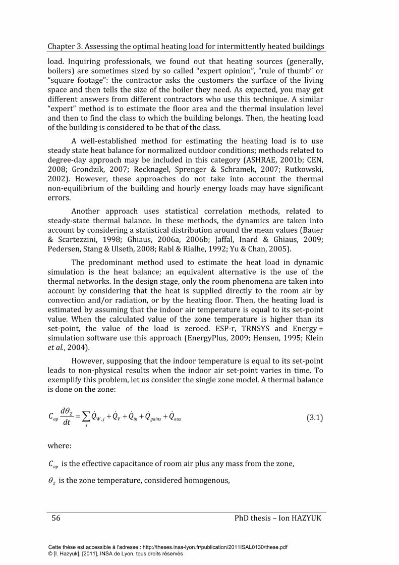
Chapter 3. Assessing the optimal heating load for intermittently heated buildings
56 PhD thesis – Ion HAZYUK
load. Inquiring professionals, we found out that heating sources (generally, boilers) are sometimes sized by so called “expert opinion”, “rule of thumb” or “square footage”: the contractor asks the customers the surface of the living space and then tells the size of the boiler they need. As expected, you may get different answers from different contractors who use this technique. A similar “expert” method is to estimate the floor area and the thermal insulation level and then to find the class to which the building belongs. Then, the heating load of the building is considered to be that of the class.
A well-established method for estimating the heating load is to use steady state heat balance for normalized outdoor conditions; methods related to degree-day approach may be included in this category (ASHRAE, 2001b; CEN, 2008; Grondzik, 2007; Recknagel, Sprenger & Schramek, 2007; Rutkowski, 2002). However, these approaches do not take into account the thermal non-equilibrium of the building and hourly energy loads may have significant errors.
Another approach uses statistical correlation methods, related to steady-state thermal balance. In these methods, the dynamics are taken into account by considering a statistical distribution around the mean values (Bauer & Scartezzini, 1998; Ghiaus, 2006a, 2006b; Jaffal, Inard & Ghiaus, 2009; Pedersen, Stang & Ulseth, 2008; Rabl & Rialhe, 1992; Yu & Chan, 2005).
The predominant method used to estimate the heat load in dynamic simulation is the heat balance; an equivalent alternative is the use of the thermal networks. In the design stage, only the room phenomena are taken into account by considering that the heat is supplied directly to the room air by convection and/or radiation, or by the heating floor. Then, the heating load is estimated by assuming that the indoor air temperature is equal to its set-point value. When the calculated value of the zone temperature is higher than its set-point, the value of the load is zeroed. ESP-r, TRNSYS and Energy + simulation software use this approach (EnergyPlus, 2009; Hensen, 1995; Klein et al., 2004).
However, supposing that the indoor temperature is equal to its set-point leads to non-physical results when the indoor air set-point varies in time. To exemplify this problem, let us consider the single zone model. A thermal balance is done on the zone:
auxgainsinVj
jWZ
ap QQQQQdt
dC ++++=∑ ,θ (3.1)
where:
apC is the effective capacitance of room air plus any mass from the zone,
Zθ is the zone temperature, considered homogenous,
Cette thèse est accessible à l'adresse : http://theses.insa-lyon.fr/publication/2011ISAL0130/these.pdf © [I. Hazyuk], [2011], INSA de Lyon, tous droits réservés
Chapter 3. Assessing the optimal heating load for intermittently heated buildings
PhD thesis – Ion HAZYUK 57
∑j
jWQ , is the sum of the heat fluxes from the interior walls to the room air,
inV QQ + are the heat fluxes from ventilation and infiltration, respectively,
auxgains QQ + are the free gains and the auxiliary gains, respectively,
The right hand side of equation (3.1) is a sum of heat fluxes. The heat flux from the interior walls, ∑
jjWQ ,
, depend on the temperature difference between
the zone, Zθ , and the wall surfaces, js,θ . Wall surface temperatures are function of the outdoor air temperature, oθ , and incident solar gains, SQ , through the transfer function of the walls. The heat fluxes due to ventilation and air infiltration are proportional to the temperature difference between the zone, zθ , and the source of air, Vθ and oθ and the wind velocity, W ; the proportionality constants are the ventilation air mass flow (an input variable) and the infiltration air mass flow (which is dependent on the outdoor air wind speed and building permeability). The free gains, gainsQ , are generally from occupants, electrical devices and direct solar gains. The auxiliary gain, auxQ , is the heat flux that the heating system needs to supply to the zone in order to maintain the indoor temperature at the set-point value. Expressing the right side terms in equation (3.1), we obtain the thermal model of a building (Figure 3-1).
Figure 3-1. Building thermal model
If we assume zero initial conditions, by applying Laplace transform to equation (3.1) we obtain
auxgainsinVj
zjsajWzap QQQQHsC ++++−=∑ )( ,, θθθ (3.2)
where:
Cette thèse est accessible à l'adresse : http://theses.insa-lyon.fr/publication/2011ISAL0130/these.pdf © [I. Hazyuk], [2011], INSA de Lyon, tous droits réservés
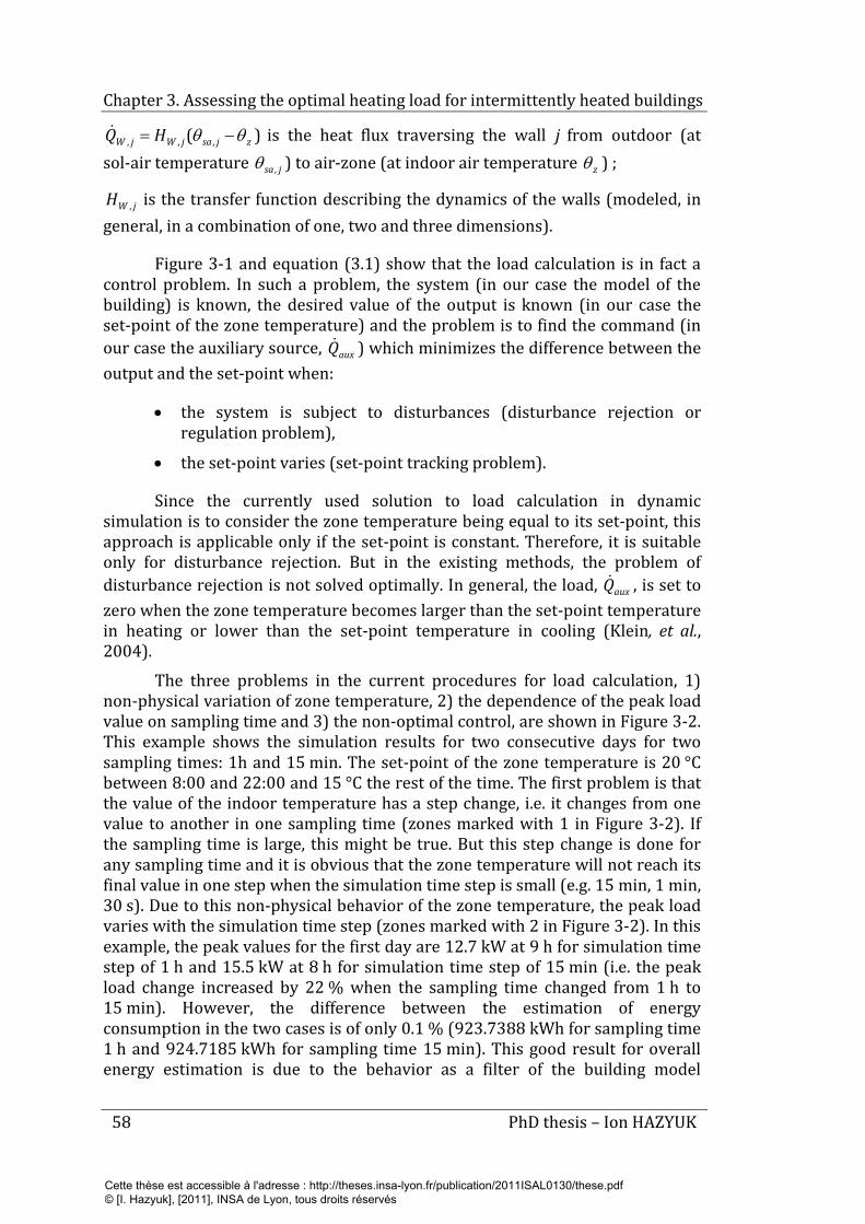
Chapter 3. Assessing the optimal heating load for intermittently heated buildings
58 PhD thesis – Ion HAZYUK
)( ,,, zjsajWjW HQ θθ −= is the heat flux traversing the wall j from outdoor (at sol-air temperature jsa ,θ ) to air-zone (at indoor air temperature zθ ) ;
jWH , is the transfer function describing the dynamics of the walls (modeled, in general, in a combination of one, two and three dimensions).
Figure 3-1 and equation (3.1) show that the load calculation is in fact a control problem. In such a problem, the system (in our case the model of the building) is known, the desired value of the output is known (in our case the set-point of the zone temperature) and the problem is to find the command (in our case the auxiliary source, auxQ ) which minimizes the difference between the output and the set-point when:
• the system is subject to disturbances (disturbance rejection or regulation problem),
• the set-point varies (set-point tracking problem).
Since the currently used solution to load calculation in dynamic simulation is to consider the zone temperature being equal to its set-point, this approach is applicable only if the set-point is constant. Therefore, it is suitable only for disturbance rejection. But in the existing methods, the problem of disturbance rejection is not solved optimally. In general, the load, auxQ , is set to zero when the zone temperature becomes larger than the set-point temperature in heating or lower than the set-point temperature in cooling (Klein, et al., 2004).
The three problems in the current procedures for load calculation, 1) non-physical variation of zone temperature, 2) the dependence of the peak load value on sampling time and 3) the non-optimal control, are shown in Figure 3-2. This example shows the simulation results for two consecutive days for two sampling times: 1h and 15 min. The set-point of the zone temperature is 20 °C between 8:00 and 22:00 and 15 °C the rest of the time. The first problem is that the value of the indoor temperature has a step change, i.e. it changes from one value to another in one sampling time (zones marked with 1 in Figure 3-2). If the sampling time is large, this might be true. But this step change is done for any sampling time and it is obvious that the zone temperature will not reach its final value in one step when the simulation time step is small (e.g. 15 min, 1 min, 30 s). Due to this non-physical behavior of the zone temperature, the peak load varies with the simulation time step (zones marked with 2 in Figure 3-2). In this example, the peak values for the first day are 12.7 kW at 9 h for simulation time step of 1 h and 15.5 kW at 8 h for simulation time step of 15 min (i.e. the peak load change increased by 22 % when the sampling time changed from 1 h to 15 min). However, the difference between the estimation of energy consumption in the two cases is of only 0.1 % (923.7388 kWh for sampling time 1 h and 924.7185 kWh for sampling time 15 min). This good result for overall energy estimation is due to the behavior as a filter of the building model
Cette thèse est accessible à l'adresse : http://theses.insa-lyon.fr/publication/2011ISAL0130/these.pdf © [I. Hazyuk], [2011], INSA de Lyon, tous droits réservés
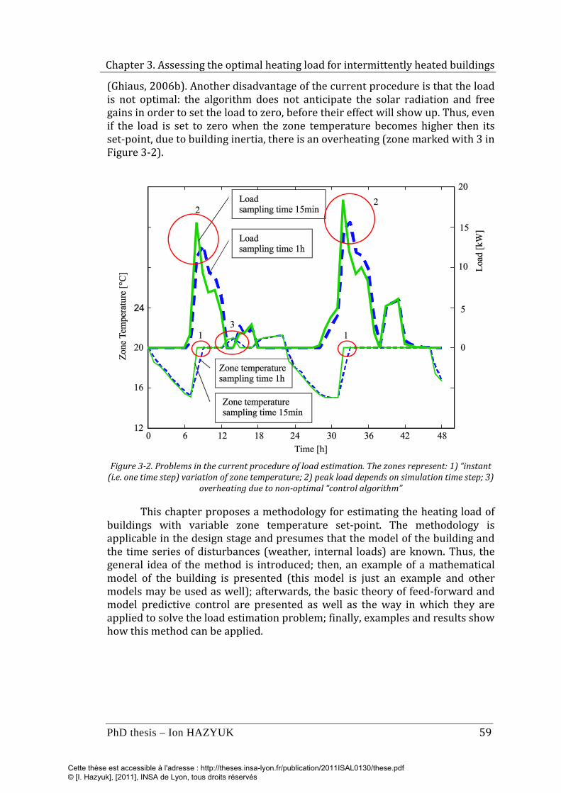
Chapter 3. Assessing the optimal heating load for intermittently heated buildings
PhD thesis – Ion HAZYUK 59
(Ghiaus, 2006b). Another disadvantage of the current procedure is that the load is not optimal: the algorithm does not anticipate the solar radiation and free gains in order to set the load to zero, before their effect will show up. Thus, even if the load is set to zero when the zone temperature becomes higher then its set-point, due to building inertia, there is an overheating (zone marked with 3 in Figure 3-2).
Figure 3-2. Problems in the current procedure of load estimation. The zones represent: 1) “instant
(i.e. one time step) variation of zone temperature; 2) peak load depends on simulation time step; 3) overheating due to non-optimal “control algorithm”
This chapter proposes a methodology for estimating the heating load of buildings with variable zone temperature set-point. The methodology is applicable in the design stage and presumes that the model of the building and the time series of disturbances (weather, internal loads) are known. Thus, the general idea of the method is introduced; then, an example of a mathematical model of the building is presented (this model is just an example and other models may be used as well); afterwards, the basic theory of feed-forward and model predictive control are presented as well as the way in which they are applied to solve the load estimation problem; finally, examples and results show how this method can be applied.
Cette thèse est accessible à l'adresse : http://theses.insa-lyon.fr/publication/2011ISAL0130/these.pdf © [I. Hazyuk], [2011], INSA de Lyon, tous droits réservés
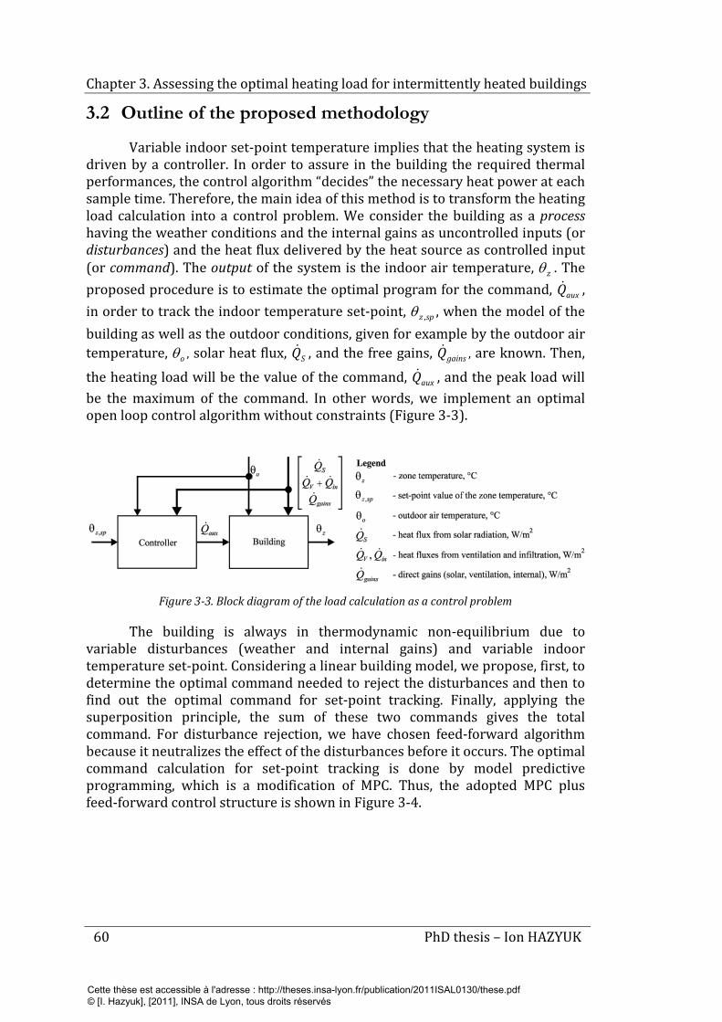
Chapter 3. Assessing the optimal heating load for intermittently heated buildings
60 PhD thesis – Ion HAZYUK
3.2 Outline of the proposed methodology
Variable indoor set-point temperature implies that the heating system is driven by a controller. In order to assure in the building the required thermal performances, the control algorithm “decides” the necessary heat power at each sample time. Therefore, the main idea of this method is to transform the heating load calculation into a control problem. We consider the building as a process having the weather conditions and the internal gains as uncontrolled inputs (or disturbances) and the heat flux delivered by the heat source as controlled input (or command). The output of the system is the indoor air temperature, zθ . The proposed procedure is to estimate the optimal program for the command, auxQ , in order to track the indoor temperature set-point, spz ,θ , when the model of the building as well as the outdoor conditions, given for example by the outdoor air temperature, oθ , solar heat flux, SQ , and the free gains, gainsQ , are known. Then, the heating load will be the value of the command, auxQ , and the peak load will be the maximum of the command. In other words, we implement an optimal open loop control algorithm without constraints (Figure 3-3).
Figure 3-3. Block diagram of the load calculation as a control problem
The building is always in thermodynamic non-equilibrium due to variable disturbances (weather and internal gains) and variable indoor temperature set-point. Considering a linear building model, we propose, first, to determine the optimal command needed to reject the disturbances and then to find out the optimal command for set-point tracking. Finally, applying the superposition principle, the sum of these two commands gives the total command. For disturbance rejection, we have chosen feed-forward algorithm because it neutralizes the effect of the disturbances before it occurs. The optimal command calculation for set-point tracking is done by model predictive programming, which is a modification of MPC. Thus, the adopted MPC plus feed-forward control structure is shown in Figure 3-4.
Cette thèse est accessible à l'adresse : http://theses.insa-lyon.fr/publication/2011ISAL0130/these.pdf © [I. Hazyuk], [2011], INSA de Lyon, tous droits réservés
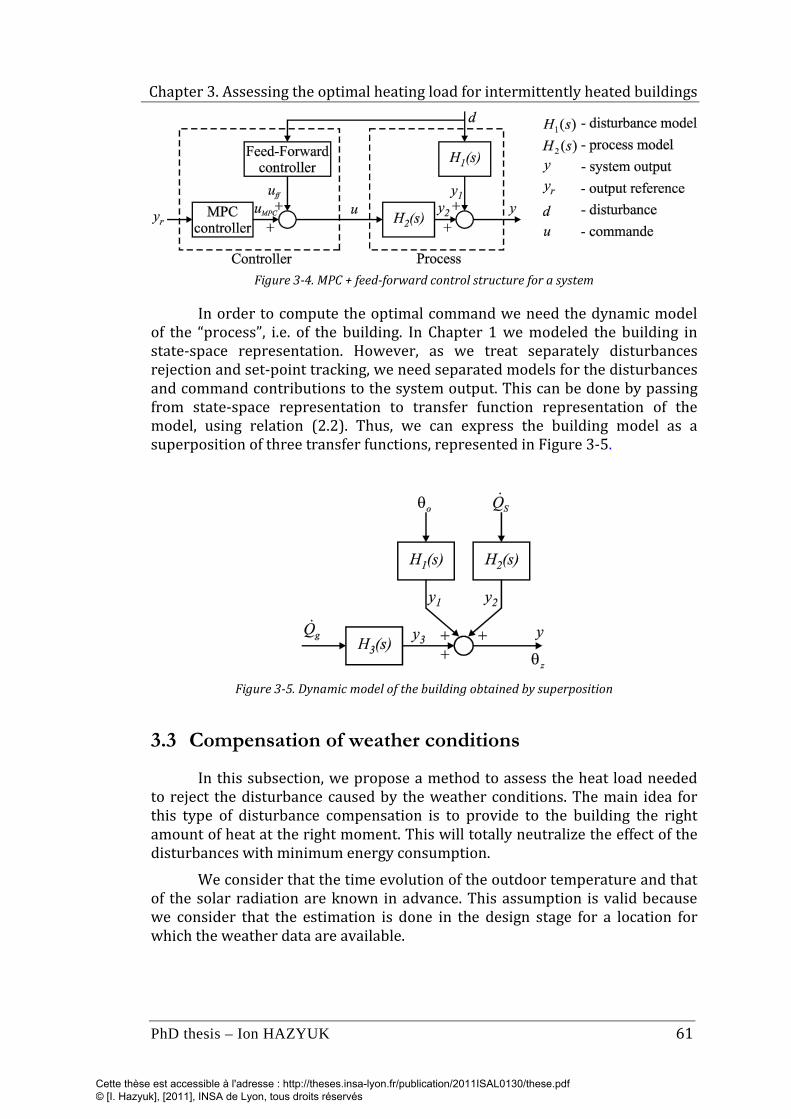
Chapter 3. Assessing the optimal heating load for intermittently heated buildings
PhD thesis – Ion HAZYUK 61
Figure 3-4. MPC + feed-forward control structure for a system
In order to compute the optimal command we need the dynamic model of the “process”, i.e. of the building. In Chapter 1 we modeled the building in state-space representation. However, as we treat separately disturbances rejection and set-point tracking, we need separated models for the disturbances and command contributions to the system output. This can be done by passing from state-space representation to transfer function representation of the model, using relation (2.2). Thus, we can express the building model as a superposition of three transfer functions, represented in Figure 3-5.
Figure 3-5. Dynamic model of the building obtained by superposition
3.3 Compensation of weather conditions
In this subsection, we propose a method to assess the heat load needed to reject the disturbance caused by the weather conditions. The main idea for this type of disturbance compensation is to provide to the building the right amount of heat at the right moment. This will totally neutralize the effect of the disturbances with minimum energy consumption.
We consider that the time evolution of the outdoor temperature and that of the solar radiation are known in advance. This assumption is valid because we consider that the estimation is done in the design stage for a location for which the weather data are available.
Cette thèse est accessible à l'adresse : http://theses.insa-lyon.fr/publication/2011ISAL0130/these.pdf © [I. Hazyuk], [2011], INSA de Lyon, tous droits réservés
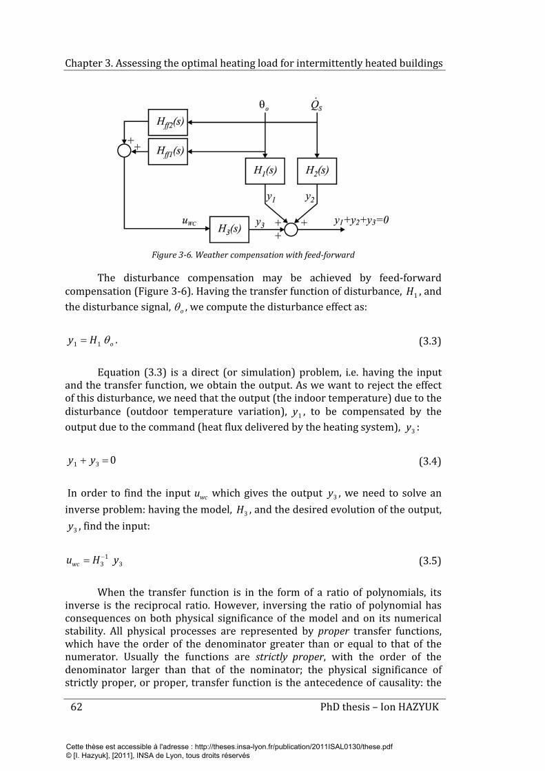
Chapter 3. Assessing the optimal heating load for intermittently heated buildings
62 PhD thesis – Ion HAZYUK
Figure 3-6. Weather compensation with feed-forward
The disturbance compensation may be achieved by feed-forward compensation (Figure 3-6). Having the transfer function of disturbance, 1H , and the disturbance signal, oθ , we compute the disturbance effect as:
oHy θ11 = . (3.3)
Equation (3.3) is a direct (or simulation) problem, i.e. having the input and the transfer function, we obtain the output. As we want to reject the effect of this disturbance, we need that the output (the indoor temperature) due to the disturbance (outdoor temperature variation), 1y , to be compensated by the output due to the command (heat flux delivered by the heating system), 3y :
031 =+ yy (3.4)
In order to find the input wcu which gives the output 3y , we need to solve an inverse problem: having the model, 3H , and the desired evolution of the output,
3y , find the input:
31
3 yHuwc−= (3.5)
When the transfer function is in the form of a ratio of polynomials, its inverse is the reciprocal ratio. However, inversing the ratio of polynomial has consequences on both physical significance of the model and on its numerical stability. All physical processes are represented by proper transfer functions, which have the order of the denominator greater than or equal to that of the numerator. Usually the functions are strictly proper, with the order of the denominator larger than that of the nominator; the physical significance of strictly proper, or proper, transfer function is the antecedence of causality: the
Cette thèse est accessible à l'adresse : http://theses.insa-lyon.fr/publication/2011ISAL0130/these.pdf © [I. Hazyuk], [2011], INSA de Lyon, tous droits réservés
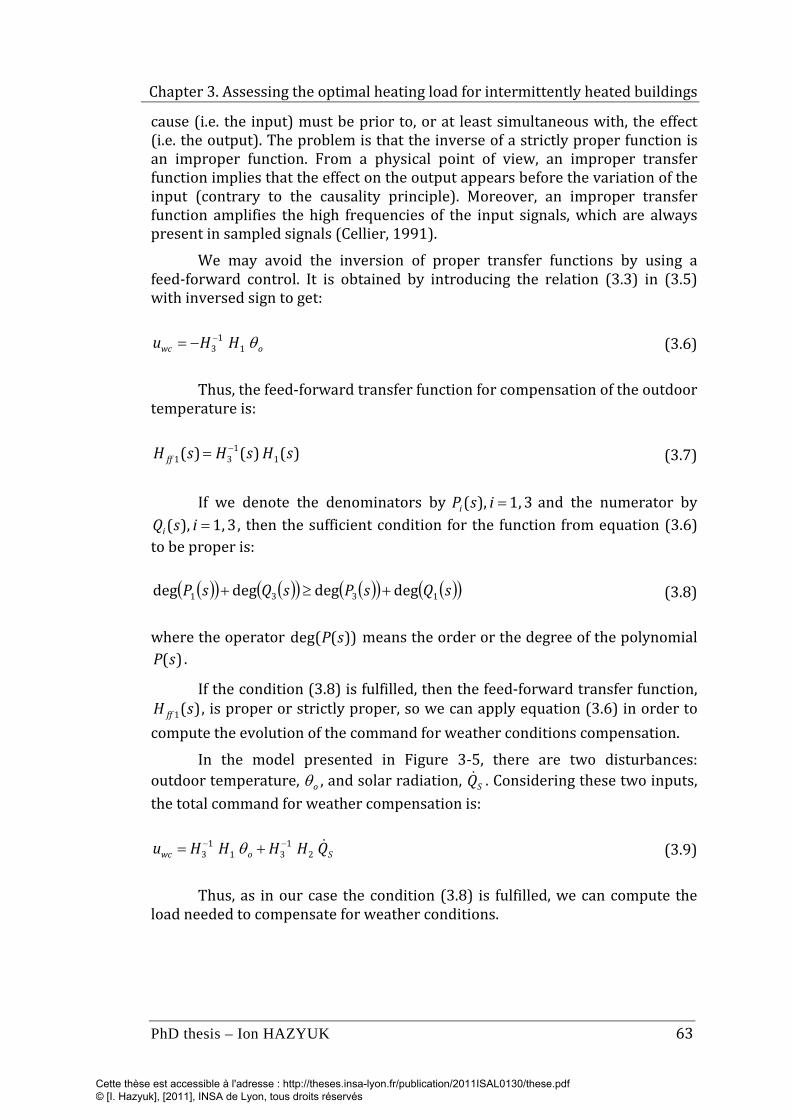
Chapter 3. Assessing the optimal heating load for intermittently heated buildings
PhD thesis – Ion HAZYUK 63
cause (i.e. the input) must be prior to, or at least simultaneous with, the effect (i.e. the output). The problem is that the inverse of a strictly proper function is an improper function. From a physical point of view, an improper transfer function implies that the effect on the output appears before the variation of the input (contrary to the causality principle). Moreover, an improper transfer function amplifies the high frequencies of the input signals, which are always present in sampled signals (Cellier, 1991).
We may avoid the inversion of proper transfer functions by using a feed-forward control. It is obtained by introducing the relation (3.3) in (3.5) with inversed sign to get:
owc HHu θ11
3−−= (3.6)
Thus, the feed-forward transfer function for compensation of the outdoor temperature is:
)()()( 11
31 sHsHsH ff−= (3.7)
If we denote the denominators by 3,1),( =isPi and the numerator by 3,1),( =isQi , then the sufficient condition for the function from equation (3.6)
to be proper is:
( )( ) ( )( ) ( )( ) ( )( )sQsPsQsP 1331 degdegdegdeg +≥+ (3.8)
where the operator ))(deg( sP means the order or the degree of the polynomial )(sP .
If the condition (3.8) is fulfilled, then the feed-forward transfer function, )(1 sH ff , is proper or strictly proper, so we can apply equation (3.6) in order to
compute the evolution of the command for weather conditions compensation.
In the model presented in Figure 3-5, there are two disturbances: outdoor temperature, oθ , and solar radiation, SQ . Considering these two inputs, the total command for weather compensation is:
Sowc QHHHHu
21
311
3−− += θ (3.9)
Thus, as in our case the condition (3.8) is fulfilled, we can compute the load needed to compensate for weather conditions.
Cette thèse est accessible à l'adresse : http://theses.insa-lyon.fr/publication/2011ISAL0130/these.pdf © [I. Hazyuk], [2011], INSA de Lyon, tous droits réservés
Chapter 3. Assessing the optimal heating load for intermittently heated buildings
64 PhD thesis – Ion HAZYUK
3.4 Set-point tracking
Inverting the transfer function for set-point tracking results in an improper transfer function. To avoid the problem of improper transfer function, we propose a solution inspired from Model Predictive Control. This approach is suitable when the program (i.e. the time evolution) of the set-point is known, which is the case when we calculate the thermal load.
3.4.1 Principles of Model Predictive Control (MPC)
We give a brief description of the principles behind MPC. An exhaustive presentation of MPC can be found in literature (Camacho & Bordons, 2004; Maciejowski, 2000; Wang, 2009). A very intuitive description from a practitioner’s point of view is also given in (Prívara, Siroký, Ferkl & Cigler, 2011).
MPC control principle is graphically illustrated in Figure 3-7. There we can find the operations that are performed between two consecutive time steps. On the top graphics there are represented the system set-point and its output, corresponding to each operation. On the bottom graphics it is represented the system command, corresponding to the output from above. Thus, the MPC principle is illustrated in three steps, each step representing a column (a pair of top-bottom graphics) in Figure 3-7.
Let us consider that we have an arbitrary set-point, whose future evolution is known in advance. Suppose that at a given discrete time step kt the system is in a given state, )( ktx , which yields an output which does not correspond to the desired set-point value. By convention, the current moment
*t is always the initial time for the controller. The first operation of MPC is to calculate a command sequence that should be applied to the system in the next
uN steps so that the system output would be forced to follow the set-point at its best in the next yN steps, while using minimal command effort. The future output is estimated using the system model and, if available, future disturbances. This operation is illustrated in Figure 3-7 (a).
The next operation of MPC is to provide the first value of the command sequence computed in the previous stage. Usually, due to modeling errors and disturbances, the output does not follow exactly its predicted evolution. Thus, at time step 1+kt there will be a one-step prediction error (Figure 3-7 b).
Cette thèse est accessible à l'adresse : http://theses.insa-lyon.fr/publication/2011ISAL0130/these.pdf © [I. Hazyuk], [2011], INSA de Lyon, tous droits réservés
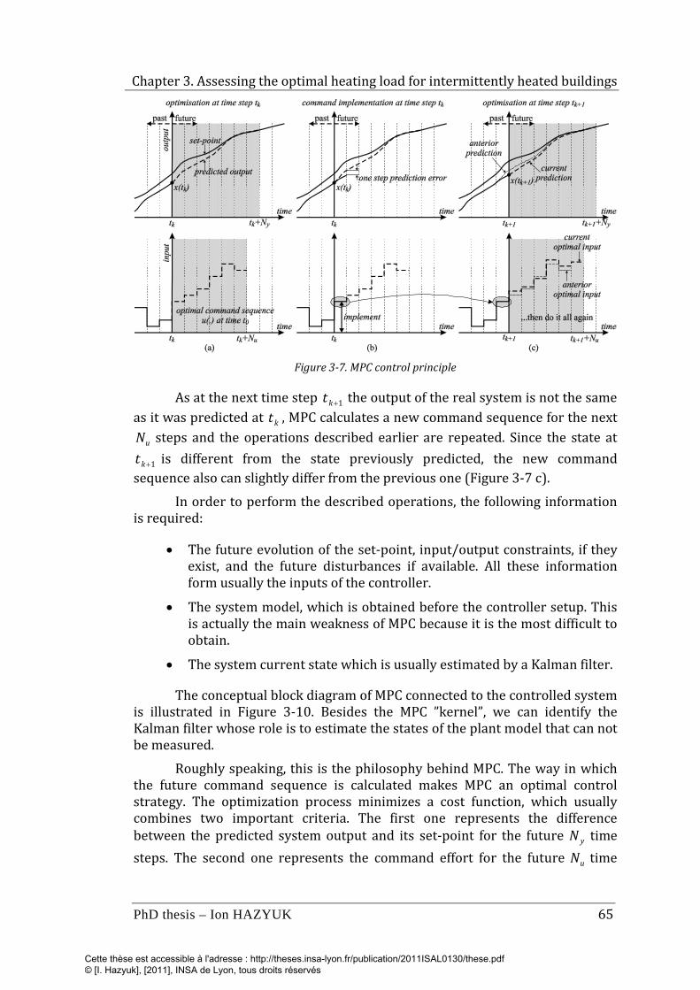
Chapter 3. Assessing the optimal heating load for intermittently heated buildings
PhD thesis – Ion HAZYUK 65
Figure 3-7. MPC control principle
As at the next time step 1+kt the output of the real system is not the same as it was predicted at kt , MPC calculates a new command sequence for the next
uN steps and the operations described earlier are repeated. Since the state at
1+kt is different from the state previously predicted, the new command sequence also can slightly differ from the previous one (Figure 3-7 c).
In order to perform the described operations, the following information is required:
• The future evolution of the set-point, input/output constraints, if they exist, and the future disturbances if available. All these information form usually the inputs of the controller.
• The system model, which is obtained before the controller setup. This is actually the main weakness of MPC because it is the most difficult to obtain.
• The system current state which is usually estimated by a Kalman filter.
The conceptual block diagram of MPC connected to the controlled system is illustrated in Figure 3-10. Besides the MPC ”kernel”, we can identify the Kalman filter whose role is to estimate the states of the plant model that can not be measured.
Roughly speaking, this is the philosophy behind MPC. The way in which the future command sequence is calculated makes MPC an optimal control strategy. The optimization process minimizes a cost function, which usually combines two important criteria. The first one represents the difference between the predicted system output and its set-point for the future yN time steps. The second one represents the command effort for the future uN time
Cette thèse est accessible à l'adresse : http://theses.insa-lyon.fr/publication/2011ISAL0130/these.pdf © [I. Hazyuk], [2011], INSA de Lyon, tous droits réservés
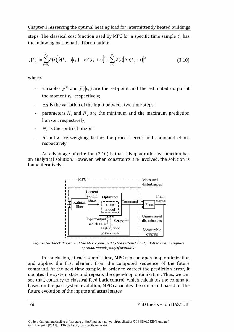
Chapter 3. Assessing the optimal heating load for intermittently heated buildings
66 PhD thesis – Ion HAZYUK
steps. The classical cost function used by MPC for a specific time sample kt has the following mathematical formulation:
[ ] [ ]∑∑==
+∆++−+=uy N
ik
N
Nik
spkkk ituiitytityitJ
1
22 )()()()(ˆ)()(1
λδ (3.10)
where:
- variables spy and )(ˆ kty ⋅ are the set-point and the estimated output at the moment kt , respectively;
- u∆ is the variation of the input between two time steps;
- parameters 1N and yN are the minimum and the maximum prediction horizon, respectively;
- uN is the control horizon;
- δ and λ are weighing factors for process error and command effort, respectively.
An advantage of criterion (3.10) is that this quadratic cost function has an analytical solution. However, when constraints are involved, the solution is found iteratively.
Figure 3-8. Block diagram of the MPC connected to the system (Plant). Dotted lines designate
optional signals, only if available.
In conclusion, at each sample time, MPC runs an open-loop optimization and applies the first element from the computed sequence of the future command. At the next time sample, in order to correct the prediction error, it updates the system state and repeats the open-loop optimization. Thus, we can see that, contrary to classical feed-back control, which calculates the command based on the past system evolution, MPC calculates the command based on the future evolution of the inputs and actual states.
Cette thèse est accessible à l'adresse : http://theses.insa-lyon.fr/publication/2011ISAL0130/these.pdf © [I. Hazyuk], [2011], INSA de Lyon, tous droits réservés
Chapter 3. Assessing the optimal heating load for intermittently heated buildings
PhD thesis – Ion HAZYUK 67
The time variation of the desired output, )(tyr , is known in advance (it is related to the set-point indoor temperature as a function of the occupational schedule of the building). Knowing the model of the system, the aim is to find the input, which minimizes the criteria given by equation (3.10). Depending on the model representation that we chose for our system, we can adopt one of existing algorithms from MPC family. We opted for an algorithm, which uses a convolution model due to several considerations:
1. The cost function from (3.10) uses the increment of the command in order to penalize control effort. Thus, to predict the output of the system, y , one needs to include an integrator in the system model. This means
an extra state in the system model and consequently additional computational time and power. On the contrary, a convolution model is directly defined between the input increment and system output, so we do not have to include the extra integrator in the process model.
2. In order to minimize the cost function (3.10), we have to invert some matrices, whose size depend on the length of the control and prediction horizons. As we want to compute a long sequence for the control, of order of days at sampling time of minutes or tens of minutes, we will have to invert large matrices. And because we have to introduce an integrator in state-space and transfer function models, the conditioning number of these matrices becomes very large (Wang, 2009). However, for convolution models, the conditioning number is smaller.
3. Convolution model can be easily obtained by simulation. Even more, when we do not have any mathematical model, we can obtain the convolution model from step or impulse response of the real system.
A MPC algorithm that uses convolution models is the Dynamic Matrix Control.
3.4.2 Principles of Dynamic Matrix Control (DMC)
Considering the step response of the system given by the following sequence:
{ }...,,,...,,,0 21 nn ssss (3.11)
where n is the number of time samples after which the system settles. We can express the system output for any input sequence by:
( ) ( ) ( )111
−−+−∆=∑=
nkuskusky n
n
ii (3.12)
Cette thèse est accessible à l'adresse : http://theses.insa-lyon.fr/publication/2011ISAL0130/these.pdf © [I. Hazyuk], [2011], INSA de Lyon, tous droits réservés
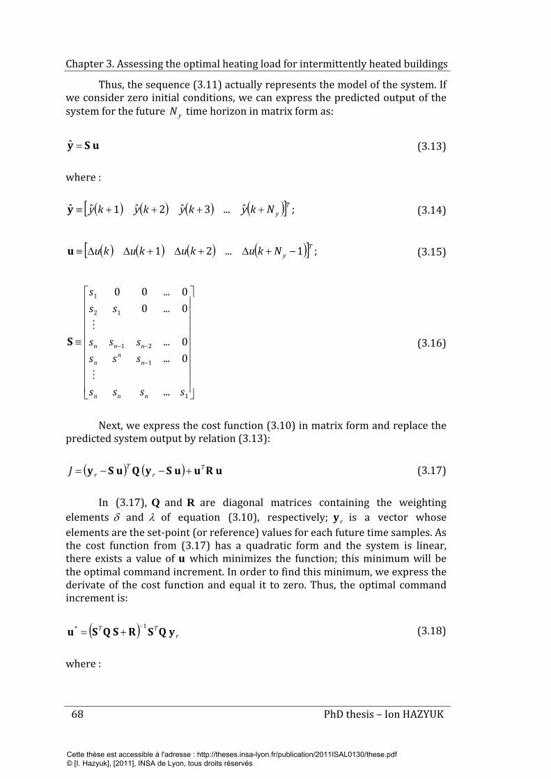
Chapter 3. Assessing the optimal heating load for intermittently heated buildings
68 PhD thesis – Ion HAZYUK
Thus, the sequence (3.11) actually represents the model of the system. If we consider zero initial conditions, we can express the predicted output of the system for the future yN time horizon in matrix form as:
uSy =ˆ (3.13)
where :
( ) ( ) ( ) ( )[ ] ;ˆ...3ˆ2ˆ1ˆˆ TyNkykykyky ++++≡y (3.14)
( ) ( ) ( ) ( )[ ] ;1...21 TyNkukukuku −+∆+∆+∆∆≡u (3.15)
≡
−
−−
1
1
21
12
1
...
0...0...
0...00...00
ssss
ssssss
sss
nnn
nn
n
nnn
S (3.16)
Next, we express the cost function (3.10) in matrix form and replace the predicted system output by relation (3.13):
( ) ( ) uRuuSyQuSy Tr
TrJ +−−= (3.17)
In (3.17), Q and R are diagonal matrices containing the weighting elements δ and λ of equation (3.10), respectively; ry is a vector whose elements are the set-point (or reference) values for each future time samples. As the cost function from (3.17) has a quadratic form and the system is linear, there exists a value of u which minimizes the function; this minimum will be the optimal command increment. In order to find this minimum, we express the derivate of the cost function and equal it to zero. Thus, the optimal command increment is:
( ) rTT yQSRSQSu 1* −
+= (3.18)
where :
Cette thèse est accessible à l'adresse : http://theses.insa-lyon.fr/publication/2011ISAL0130/these.pdf © [I. Hazyuk], [2011], INSA de Lyon, tous droits réservés
Chapter 3. Assessing the optimal heating load for intermittently heated buildings
PhD thesis – Ion HAZYUK 69
( ) ( ) ( ) ( )[ ]TyNkukukuku 1*...21 **** −+∆+∆+∆∆≡u (3.19)
Once we got the optimal incremental command, which optimizes the cost function (3.17), we compute the command sequence by:
( ) ( )∑=
∆=k
iiuku
1
* (3.20)
Thus by applying relations (3.18) and (3.20) we get the optimal command for uN future time horizon which optimizes cost function (3.17).
3.4.3 Adapting DMC for command programming
In the two previous subsections, we presented the principles of MPC and the general DMC method. In this subsection, we present some considerations on how we can apply the DMC algorithm for load calculation and how to choose the tuning parameters in order to obtain desired performances of the process.
The Dynamic Matrix Control algorithm needs measurements of the actual state of the system at each sampling moment, computes the predictive command and sends to the process the first value from the sequence. In addition, in almost all practical situations we have physical constraints on the maximal and minimal value and/or change rate of the command. These constrains also can be included into optimization function using Lagrange multipliers (Wang, 2009). Then, the computation of optimal command becomes an iterative algorithm (not presented in this thesis). However, our aim is the load calculation, not indoor temperature control. Thus, the first and most important difference between control application of MPC and MPC based load calculation is that we do not impose any constraints on the command. We compute the evolution of the command in order to find the maximal needed power for an optimal control of the heating system for a given occupational scenario. Another difference is the control horizon: since in control applications we are interested just in the first element of the computed control sequence, we do not consider large control horizons and retain only the first element of the command sequence (3.20), the rest of the sequence being neglected. On the contrary, for load calculation, we compute the optimal control sequence only once and we keep all the elements of the sequence. This open-loop approach (which does not use the feedback as in MPC) is applicable because for the load calculation we consider that the disturbances (weather conditions and occupancy) and the set-point of the indoor temperature are known and the process is the model of the building, which implies that there is no difference between the process and its model. Finally, in control applications the control horizon is usually shorter then the prediction horizon. In our case, we will consider the control horizon equal to the prediction horizon.
Cette thèse est accessible à l'adresse : http://theses.insa-lyon.fr/publication/2011ISAL0130/these.pdf © [I. Hazyuk], [2011], INSA de Lyon, tous droits réservés
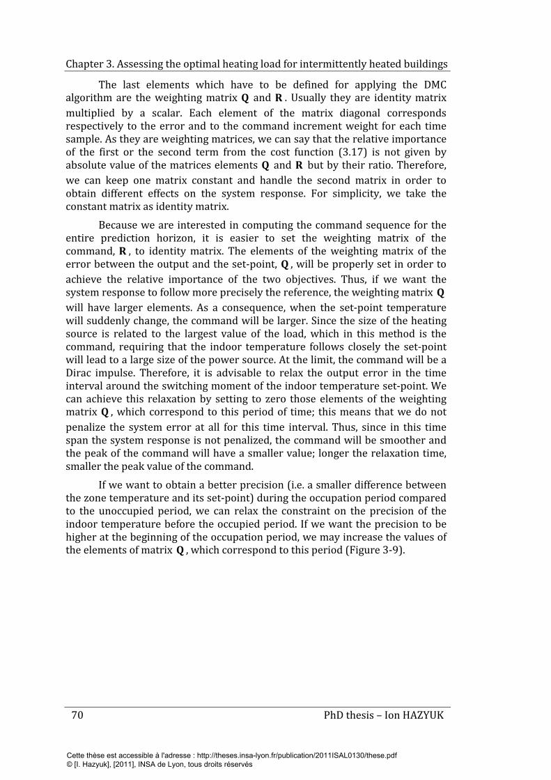
Chapter 3. Assessing the optimal heating load for intermittently heated buildings
70 PhD thesis – Ion HAZYUK
The last elements which have to be defined for applying the DMC algorithm are the weighting matrix Q and R . Usually they are identity matrix multiplied by a scalar. Each element of the matrix diagonal corresponds respectively to the error and to the command increment weight for each time sample. As they are weighting matrices, we can say that the relative importance of the first or the second term from the cost function (3.17) is not given by absolute value of the matrices elements Q and R but by their ratio. Therefore, we can keep one matrix constant and handle the second matrix in order to obtain different effects on the system response. For simplicity, we take the constant matrix as identity matrix.
Because we are interested in computing the command sequence for the entire prediction horizon, it is easier to set the weighting matrix of the command, R , to identity matrix. The elements of the weighting matrix of the error between the output and the set-point, Q , will be properly set in order to achieve the relative importance of the two objectives. Thus, if we want the system response to follow more precisely the reference, the weighting matrix Q will have larger elements. As a consequence, when the set-point temperature will suddenly change, the command will be larger. Since the size of the heating source is related to the largest value of the load, which in this method is the command, requiring that the indoor temperature follows closely the set-point will lead to a large size of the power source. At the limit, the command will be a Dirac impulse. Therefore, it is advisable to relax the output error in the time interval around the switching moment of the indoor temperature set-point. We can achieve this relaxation by setting to zero those elements of the weighting matrix Q , which correspond to this period of time; this means that we do not penalize the system error at all for this time interval. Thus, since in this time span the system response is not penalized, the command will be smoother and the peak of the command will have a smaller value; longer the relaxation time, smaller the peak value of the command.
If we want to obtain a better precision (i.e. a smaller difference between the zone temperature and its set-point) during the occupation period compared to the unoccupied period, we can relax the constraint on the precision of the indoor temperature before the occupied period. If we want the precision to be higher at the beginning of the occupation period, we may increase the values of the elements of matrix Q , which correspond to this period (Figure 3-9).
Cette thèse est accessible à l'adresse : http://theses.insa-lyon.fr/publication/2011ISAL0130/these.pdf © [I. Hazyuk], [2011], INSA de Lyon, tous droits réservés
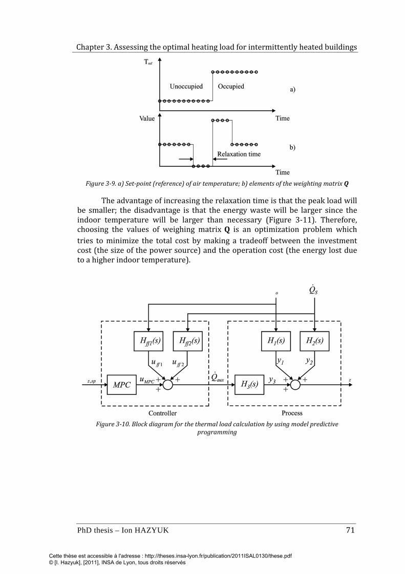
Chapter 3. Assessing the optimal heating load for intermittently heated buildings
PhD thesis – Ion HAZYUK 71
Figure 3-9. a) Set-point (reference) of air temperature; b) elements of the weighting matrix Q
The advantage of increasing the relaxation time is that the peak load will be smaller; the disadvantage is that the energy waste will be larger since the indoor temperature will be larger than necessary (Figure 3-11). Therefore, choosing the values of weighing matrix Q is an optimization problem which tries to minimize the total cost by making a tradeoff between the investment cost (the size of the power source) and the operation cost (the energy lost due to a higher indoor temperature).
Figure 3-10. Block diagram for the thermal load calculation by using model predictive
programming
Cette thèse est accessible à l'adresse : http://theses.insa-lyon.fr/publication/2011ISAL0130/these.pdf © [I. Hazyuk], [2011], INSA de Lyon, tous droits réservés
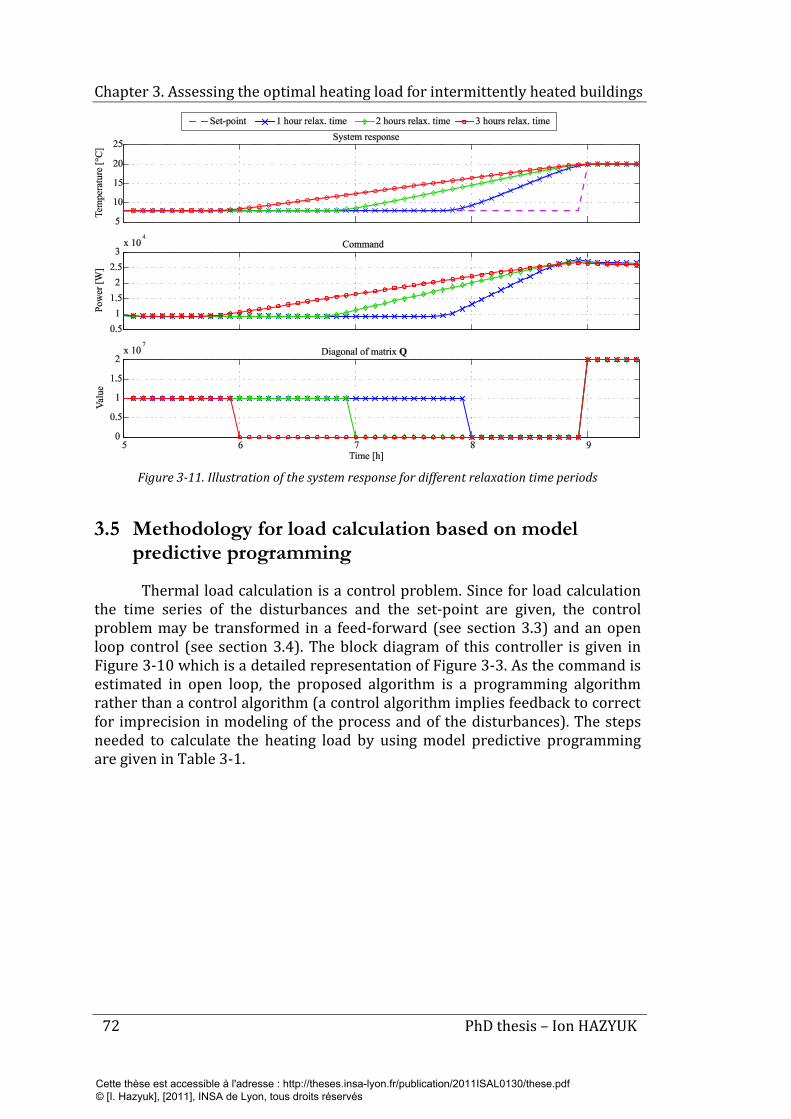
Chapter 3. Assessing the optimal heating load for intermittently heated buildings
72 PhD thesis – Ion HAZYUK
Figure 3-11. Illustration of the system response for different relaxation time periods
3.5 Methodology for load calculation based on model predictive programming
Thermal load calculation is a control problem. Since for load calculation the time series of the disturbances and the set-point are given, the control problem may be transformed in a feed-forward (see section 3.3) and an open loop control (see section 3.4). The block diagram of this controller is given in Figure 3-10 which is a detailed representation of Figure 3-3. As the command is estimated in open loop, the proposed algorithm is a programming algorithm rather than a control algorithm (a control algorithm implies feedback to correct for imprecision in modeling of the process and of the disturbances). The steps needed to calculate the heating load by using model predictive programming are given in Table 3-1.
Cette thèse est accessible à l'adresse : http://theses.insa-lyon.fr/publication/2011ISAL0130/these.pdf © [I. Hazyuk], [2011], INSA de Lyon, tous droits réservés

Chapter 3. Assessing the optimal heating load for intermittently heated buildings
PhD thesis – Ion HAZYUK 73
Table 3-1. Procedure for load calculation by using model predictive programming
Step Action
1 Find the dynamic model of the building in the form of transfer functions (Figure 3-5).
2 Chose representative weather conditions and profile of the indoor temperature set-point:
for total load estimation chose the whole heating season
for maximal load estimation chose the worse period
3 Find the initial conditions by repeating the simulation for the same 24h interval until permanent regime is attained.
4 Compute the evolution of needed power to compensate weather conditions using feed-forward (equation (3.9)).
5 Choose the weighting matrix Q (Figure 3-9).
6 Use model predictive programming to compute the evolution of power needed for tracking the set-point temperature (relations (3.18) and (3.20)).
7 Sum the time series of heat power (i.e. command sequence) for weather compensation with the time series of heat power (i.e. command sequence) for set-point tracking to get the total power.
8 Choose the maximal value of the command to obtain the maximum load.
3.6 Examples and discussions
As an example, let us consider a three-storey building having the footprint area of 100 m². The values of the thermal parameters estimated during the design of the building are given in Table 3-2.
Cette thèse est accessible à l'adresse : http://theses.insa-lyon.fr/publication/2011ISAL0130/these.pdf © [I. Hazyuk], [2011], INSA de Lyon, tous droits réservés
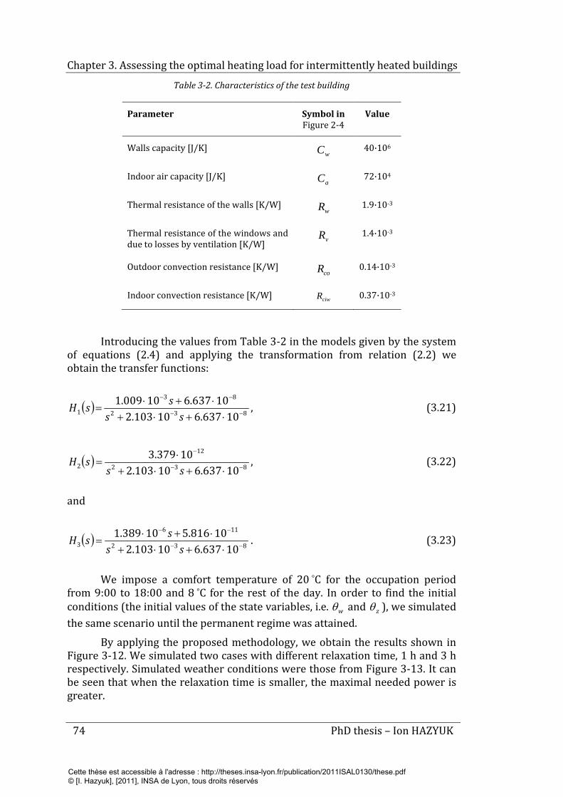
Chapter 3. Assessing the optimal heating load for intermittently heated buildings
74 PhD thesis – Ion HAZYUK
Table 3-2. Characteristics of the test building
Parameter Symbol in Figure 2-4
Value
Walls capacity [J/K] wC 40·106
Indoor air capacity [J/K] aC 72·104
Thermal resistance of the walls [K/W] wR 1.9·10-3
Thermal resistance of the windows and due to losses by ventilation [K/W] vR 1.4·10-3
Outdoor convection resistance [K/W] coR 0.14·10-3
Indoor convection resistance [K/W] ciwR 0.37·10-3
Introducing the values from Table 3-2 in the models given by the system of equations (2.4) and applying the transformation from relation (2.2) we obtain the transfer functions:
( ) 832
83
1 10637.610103.210637.610009.1
−−
−−
⋅+⋅+⋅+⋅
=ss
ssH , (3.21)
( ) 832
12
2 10637.610103.210379.3
−−
−
⋅+⋅+⋅
=ss
sH , (3.22)
and
( ) 832
116
3 10637.610103.210816.510389.1
−−
−−
⋅+⋅+⋅+⋅
=ss
ssH . (3.23)
We impose a comfort temperature of 20 °C for the occupation period from 9:00 to 18:00 and 8 °C for the rest of the day. In order to find the initial conditions (the initial values of the state variables, i.e. wθ and zθ ), we simulated the same scenario until the permanent regime was attained.
By applying the proposed methodology, we obtain the results shown in Figure 3-12. We simulated two cases with different relaxation time, 1 h and 3 h respectively. Simulated weather conditions were those from Figure 3-13. It can be seen that when the relaxation time is smaller, the maximal needed power is greater.
Cette thèse est accessible à l'adresse : http://theses.insa-lyon.fr/publication/2011ISAL0130/these.pdf © [I. Hazyuk], [2011], INSA de Lyon, tous droits réservés
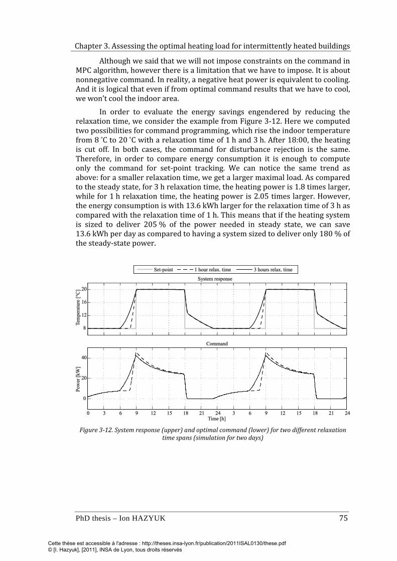
Chapter 3. Assessing the optimal heating load for intermittently heated buildings
PhD thesis – Ion HAZYUK 75
Although we said that we will not impose constraints on the command in MPC algorithm, however there is a limitation that we have to impose. It is about nonnegative command. In reality, a negative heat power is equivalent to cooling. And it is logical that even if from optimal command results that we have to cool, we won’t cool the indoor area.
In order to evaluate the energy savings engendered by reducing the relaxation time, we consider the example from Figure 3-12. Here we computed two possibilities for command programming, which rise the indoor temperature from 8 °C to 20 °C with a relaxation time of 1 h and 3 h. After 18:00, the heating is cut off. In both cases, the command for disturbance rejection is the same. Therefore, in order to compare energy consumption it is enough to compute only the command for set-point tracking. We can notice the same trend as above: for a smaller relaxation time, we get a larger maximal load. As compared to the steady state, for 3 h relaxation time, the heating power is 1.8 times larger, while for 1 h relaxation time, the heating power is 2.05 times larger. However, the energy consumption is with 13.6 kWh larger for the relaxation time of 3 h as compared with the relaxation time of 1 h. This means that if the heating system is sized to deliver 205 % of the power needed in steady state, we can save 13.6 kWh per day as compared to having a system sized to deliver only 180 % of the steady-state power.
Figure 3-12. System response (upper) and optimal command (lower) for two different relaxation
time spans (simulation for two days)
Cette thèse est accessible à l'adresse : http://theses.insa-lyon.fr/publication/2011ISAL0130/these.pdf © [I. Hazyuk], [2011], INSA de Lyon, tous droits réservés
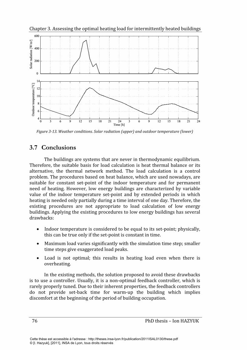
Chapter 3. Assessing the optimal heating load for intermittently heated buildings
76 PhD thesis – Ion HAZYUK
Figure 3-13. Weather conditions. Solar radiation (upper) and outdoor temperature (lower)
3.7 Conclusions
The buildings are systems that are never in thermodynamic equilibrium. Therefore, the suitable basis for load calculation is heat thermal balance or its alternative, the thermal network method. The load calculation is a control problem. The procedures based on heat balance, which are used nowadays, are suitable for constant set-point of the indoor temperature and for permanent need of heating. However, low energy buildings are characterized by variable value of the indoor temperature set-point and by extended periods in which heating is needed only partially during a time interval of one day. Therefore, the existing procedures are not appropriate to load calculation of low energy buildings. Applying the existing procedures to low energy buildings has several drawbacks:
• Indoor temperature is considered to be equal to its set-point; physically, this can be true only if the set-point is constant in time.
• Maximum load varies significantly with the simulation time step; smaller time steps give exaggerated load peaks.
• Load is not optimal; this results in heating load even when there is overheating.
In the existing methods, the solution proposed to avoid these drawbacks is to use a controller. Usually, it is a non-optimal feedback controller, which is rarely properly tuned. Due to their inherent properties, the feedback controllers do not provide set-back time for warm-up the building which implies discomfort at the beginning of the period of building occupation.
Cette thèse est accessible à l'adresse : http://theses.insa-lyon.fr/publication/2011ISAL0130/these.pdf © [I. Hazyuk], [2011], INSA de Lyon, tous droits réservés
Chapter 3. Assessing the optimal heating load for intermittently heated buildings
PhD thesis – Ion HAZYUK 77
During the design stage, a dynamic model of the building is available as well as the time series of the weather conditions and of the set-point indoor temperature. This gives the opportunity to find out an optimal program for the power needed by the building in order to reject the disturbances and to track the set-point. The solution proposed in this section is a combination of feed-forward compensation of weather disturbances and model predictive programming which is obtained by modifying the dynamic matrix control (DMC), a variant of model predictive control (MPC), for set-point tracking. This algorithm rejects the disturbances and gives the keys to unconstrained optimal set-point tracking and control command effort. Solving the problem of optimal set-point tracking needs the specification of the weighting matrix for output error (i.e. the difference between the set-point and the indoor temperature) and for command effort. This chapter proposes to set the weight matrix of the command to unity and to treat only the weighting matrix of the output error. Then, the values of the weighting matrix of the error are obtained by defining the duration of a relaxation time before the set-point change (i.e. the setback time), in which we accept larger values of the output error, and a reinforcing time at the beginning of the occupation period, in which the output error is forced to be low. The choice of these values needs to be done by considering investment and operation costs. Lower output error implies higher peak load, thus higher power of the installed heating system, but lower energy consumption. The tuning of the weighting matrix of the output error, based on these economical considerations, is not treated in this chapter.
Cette thèse est accessible à l'adresse : http://theses.insa-lyon.fr/publication/2011ISAL0130/these.pdf © [I. Hazyuk], [2011], INSA de Lyon, tous droits réservés
Chapter 3. Assessing the optimal heating load for intermittently heated buildings
78 PhD thesis – Ion HAZYUK
References
ASHRAE (2001a). Energy estimating and modeling methods. Chapter 31 in: 2001 ASHRAE Fundamentals Handbook. Atlanta, GA: American Society of Heating, Refrigerating, and Air-Conditioning Engineers.
ASHRAE (2001b). Residential cooling and heating load calculations. Chapter 28 in: 2001 ASHRAE Fundamentals Handbook. Atlanta, GA: American Society of Heating, Refrigerating, and Air-Conditioning Engineers.
Bauer, M. & Scartezzini, J. L. (1998). A simplified correlation method accounting for heating and cooling loads in energy-efficient buildings. Energy and Buildings, 27(2), 147-154.
Camacho, E. F. & Bordons, A. C. (2004). Model Predictive Control (2nd ed.). London: Springer-Verlag.
Cellier, F. E. (1991). Continuous System Modeling. New York, NY: Springer-Verlag.
CEN (2008). EN ISO 13790:2008: Energy performance of buildings - Calculation of energy use for space heating and cooling. Brussels, Belgium: European Committee for Standardization.
EnergyPlus (2009). EnergyPlus Engineering Reference: The Reference to EnergyPlus Calculations: Lawrence Berkeley National Laboratory.
Ghiaus, C. (2006a). Equivalence between the load curve and the free-running temperature in energy estimating methods. Energy and Buildings, 38(5), 429-435.
Ghiaus, C. (2006b). Experimental estimation of building energy performance by robust regression. Energy and Buildings, 38(6), 582-587.
Grondzik, W. T. (Ed.). (2007). Air-Conditioning System Design Manual (2nd ed.). Burlington, MA: Butterworth-Heinemann
Hensen, J. L. M. (1995). On system simulation for building performance evaluation. In: 4th IBPSA World Congress "Building Simulation '95", August 14-16, 1995, Madison, WI, USA.
Jaffal, I., Inard, C. & Ghiaus, C. (2009). Fast method to predict building heating demand based on the design of experiments. Energy and Buildings, 41(6), 669-677.
Klein, S. A., Beckman, W. A., Mitchell, J. W., Duffie, J. A., Duffie, N. A., Freeman, T. L., et al. (2004). TRNSYS 16 - Mathematical reference (Vol. 5): Solar Energy Laboratory, University of Wisconsin-Madison.
Maciejowski, J. M. (2000). Predictive Control with Constraints. London: Prentice Hall.
Cette thèse est accessible à l'adresse : http://theses.insa-lyon.fr/publication/2011ISAL0130/these.pdf © [I. Hazyuk], [2011], INSA de Lyon, tous droits réservés
Chapter 3. Assessing the optimal heating load for intermittently heated buildings
PhD thesis – Ion HAZYUK 79
Pedersen, L., Stang, J. & Ulseth, R. (2008). Load prediction method for heat and electricity demand in buildings for the purpose of planning for mixed energy distribution systems. Energy and Buildings, 40(7), 1124-1134.
Prívara, S., Siroký, J., Ferkl, L. & Cigler, J. (2011). Model predictive control of a building heating system: The first experience. Energy and Buildings, 43(2-3), 564-572.
Rabl, A. & Rialhe, A. (1992). Energy signature models for commercial buildings: test with measured data and interpretation. Energy and Buildings, 19(2), 143-154.
Recknagel, H., Sprenger, E. & Schramek, E.-R. (2007). Calcul et dimensionnement des installations de chauffage. Chapter in: Génie Climatique: Dunod.
Rutkowski, H. (2002). Manual J – Residential Load Calculation (8th ed.). Arlington, VA: Air Conditioning Contractors of America.
Wang, L. (2009). Model Predictive Control System Design and Implementation using MATLAB. London: Springer-Verlag.
Yu, F. W. & Chan, K. T. (2005). Energy signatures for assessing the energy performance of chillers. Energy and Buildings, 37(7), 739-746.
Cette thèse est accessible à l'adresse : http://theses.insa-lyon.fr/publication/2011ISAL0130/these.pdf © [I. Hazyuk], [2011], INSA de Lyon, tous droits réservés

Cette thèse est accessible à l'adresse : http://theses.insa-lyon.fr/publication/2011ISAL0130/these.pdf © [I. Hazyuk], [2011], INSA de Lyon, tous droits réservés
81
Chapter 4
Temperature control
The goal of optimal control is to assure thermal comfort with minimal energy consumption. Of particular interest is the set-point tracking in intermittently heated buildings, and especially the set-back time to warm-up the building when the heating system is shut or slowed down during the night periods. Model Predictive Control (MPC) is considered one of the best candidate for this task due to its ability to use the occupancy schedule and weather forecasts for optimal temperature control. However, the classical formulation of the MPC cost function is not adequately formulated for minimizing thermal energy consumption. Therefore, we introduce a new criterion, which optimizes the energy in thermal systems, and we propose Linear Programming (LP) for solving this optimization problem.
4.1 Introduction
In this chapter, we focus on the development of a Model Predictive Controller (MPC) for hydronic heating systems working intermittently. MPC needs the model of the process and in Chapter 2 we proposed a low order thermal model for which the parameters are obtained by identification. We also have shown that the input-output relation between the temperature of the inlet water of the radiator (controlled input of the model) and the indoor temperature (the output of the model) is nonlinear and we determined the static nonlinearity. In this chapter, we first analyze the performance requirements, current control practices and MPC performances reported in literature for thermal control of building. Then, we suggest a cost function with a true energy meaning for the thermal systems. We give a solution for solving the optimization problem by using Linear Programming (LP). We show how to linearize the thermal model of the building by inverting its static characteristic.
Cette thèse est accessible à l'adresse : http://theses.insa-lyon.fr/publication/2011ISAL0130/these.pdf © [I. Hazyuk], [2011], INSA de Lyon, tous droits réservés
Chapter 4. Temperature control
82 PhD thesis – Ion HAZYUK
At this stage, we consider that the hydronic heating system can deliver immediately water at the temperature calculated by the MPC algorithm. If the heating source (such as boilers, heat pumps, etc) is taken into account, a delay may occur between the request and the delivery of the hot water. This case, where the whole heating system is considered, is treated later, in Chapter 5.
4.2 Temperature control in buildings
Control theory is a vast research area which gives us an important number of controller types to perform automatic control. The choice of a controller must be performed by analyzing several factors, among which is the type of the desired performance. In intermittent heated buildings, temperature stabilization and disturbance rejection is not enough; we need to assure the comfort, i.e. to not have temperatures below the lower accepted limit during heating season, and to consume minimum energy. These particular performances are discussed hereafter.
4.2.1 Usual requirements in intermittently heated buildings
Energy savings can be achieved by adopting an intermittent heating strategy. However, a comfortable environment for the inhabitants must be assured. The thermal comfort is related to occupants’ health and productivity. Usually, if the comfort in the building is not assured, people improvise. When it is too hot they open the windows instead of lowering the temperature set-point or they use non-controlled backup heating sources when it is repeatedly cold. All these actions increase the energy consumption, which contradicts the initial objective – that of energy savings.
Thermal comfort in buildings is influenced by several factors like temperature, relative humidity and velocity of the ambient air, mean radiant temperature, but also by clothing, person activity and metabolic rate. Fanger (1972) defined comfort indexes as PMV (Predicted Mean Vote) and PPD (Predicted Percent of Dissatisfied People), which today are used in European thermal regulations (CEN, 2005). ASHRAE Standard 55 (ASHRAE, 2004) defines a comfortable ambiance as being rather a comfort zone instead of a particular thermal environment. This zone (Figure 4-1), corresponds to 80 % of occupants’ acceptability, i.e. 20 % PPD, or, (-0.5 +0.5) range of PMV.
Cette thèse est accessible à l'adresse : http://theses.insa-lyon.fr/publication/2011ISAL0130/these.pdf © [I. Hazyuk], [2011], INSA de Lyon, tous droits réservés
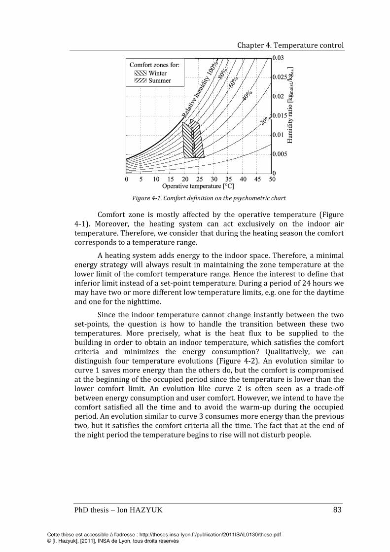
Chapter 4. Temperature control
PhD thesis – Ion HAZYUK 83
Figure 4-1. Comfort definition on the psychometric chart
Comfort zone is mostly affected by the operative temperature (Figure 4-1). Moreover, the heating system can act exclusively on the indoor air temperature. Therefore, we consider that during the heating season the comfort corresponds to a temperature range.
A heating system adds energy to the indoor space. Therefore, a minimal energy strategy will always result in maintaining the zone temperature at the lower limit of the comfort temperature range. Hence the interest to define that inferior limit instead of a set-point temperature. During a period of 24 hours we may have two or more different low temperature limits, e.g. one for the daytime and one for the nighttime.
Since the indoor temperature cannot change instantly between the two set-points, the question is how to handle the transition between these two temperatures. More precisely, what is the heat flux to be supplied to the building in order to obtain an indoor temperature, which satisfies the comfort criteria and minimizes the energy consumption? Qualitatively, we can distinguish four temperature evolutions (Figure 4-2). An evolution similar to curve 1 saves more energy than the others do, but the comfort is compromised at the beginning of the occupied period since the temperature is lower than the lower comfort limit. An evolution like curve 2 is often seen as a trade-off between energy consumption and user comfort. However, we intend to have the comfort satisfied all the time and to avoid the warm-up during the occupied period. An evolution similar to curve 3 consumes more energy than the previous two, but it satisfies the comfort criteria all the time. The fact that at the end of the night period the temperature begins to rise will not disturb people.
Cette thèse est accessible à l'adresse : http://theses.insa-lyon.fr/publication/2011ISAL0130/these.pdf © [I. Hazyuk], [2011], INSA de Lyon, tous droits réservés
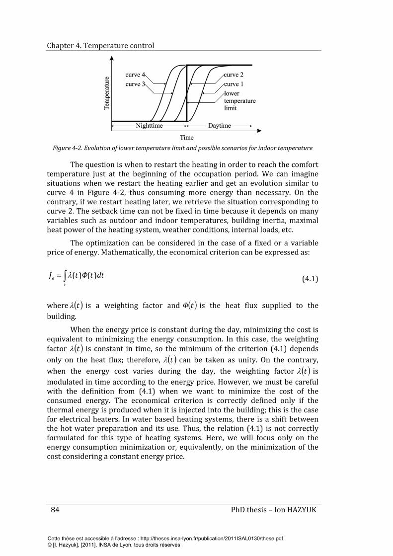
Chapter 4. Temperature control
84 PhD thesis – Ion HAZYUK
Figure 4-2. Evolution of lower temperature limit and possible scenarios for indoor temperature
The question is when to restart the heating in order to reach the comfort temperature just at the beginning of the occupation period. We can imagine situations when we restart the heating earlier and get an evolution similar to curve 4 in Figure 4-2, thus consuming more energy than necessary. On the contrary, if we restart heating later, we retrieve the situation corresponding to curve 2. The setback time can not be fixed in time because it depends on many variables such as outdoor and indoor temperatures, building inertia, maximal heat power of the heating system, weather conditions, internal loads, etc.
The optimization can be considered in the case of a fixed or a variable price of energy. Mathematically, the economical criterion can be expressed as:
dttΦtJt
e ∫= )()(λ (4.1)
where ( )tλ is a weighting factor and ( )tΦ is the heat flux supplied to the building.
When the energy price is constant during the day, minimizing the cost is equivalent to minimizing the energy consumption. In this case, the weighting factor ( )tλ is constant in time, so the minimum of the criterion (4.1) depends only on the heat flux; therefore, ( )tλ can be taken as unity. On the contrary, when the energy cost varies during the day, the weighting factor ( )tλ is modulated in time according to the energy price. However, we must be careful with the definition from (4.1) when we want to minimize the cost of the consumed energy. The economical criterion is correctly defined only if the thermal energy is produced when it is injected into the building; this is the case for electrical heaters. In water based heating systems, there is a shift between the hot water preparation and its use. Thus, the relation (4.1) is not correctly formulated for this type of heating systems. Here, we will focus only on the energy consumption minimization or, equivalently, on the minimization of the cost considering a constant energy price.
Cette thèse est accessible à l'adresse : http://theses.insa-lyon.fr/publication/2011ISAL0130/these.pdf © [I. Hazyuk], [2011], INSA de Lyon, tous droits réservés
Chapter 4. Temperature control
PhD thesis – Ion HAZYUK 85
Summing up, we may retain that:
• When people feel thermal discomfort, they improvise and this leads to increasing of energy consumption, even more than would be necessary to ensure a proper thermal comfort. The cost of discomfort is so high that it is advisable to avoid temperatures below the lower comfort limit.
• An acceptable comfort sensation is not just a set-point temperature but rather a comfort zone, which corresponds to a temperature range. As we are focusing only on the heating season, we retain the lower limit of the comfort temperature.
• The controller needs to maintain the indoor temperature above the lower comfort limit by consuming as less energy as possible. This means that, besides disturbance rejection, the controller must predict the restart time to attain the comfort temperature at the right moment.
4.2.2 Current practice in building thermal control
Our focus is on the emitter control. The strategies to control heat sources are presented in Chapter 5.
Since 2005, several groups of researchers have carried out surveys on the current thermal control strategies in buildings (Dounis & Caraiscos, 2009; Liao, Swainson & Dexter, 2005; Peeters, Van der Veken, Hens, Helsen & D'Haeseleer, 2008). Their surveys show that usually room thermostats and/or thermostatic valves on radiators (TVR) are used. Both controllers act on the radiator inlet water flow rate; room thermostats are on-off controllers and TVR are basically proportional controllers. In order to avoid frequent changes, the thermostats have a dead band. The survey revealed that the majority of the occupants failed to use TVR as they were designed, so they perform very poorly (Meier et al., 2010). Usually the users fail to reduce the emitted heat when it is too hot, resulting in room overheating and thus energy wasting. To solve the overheating problem, PID controllers are used on the radiator valves. These controllers improved the situation, but, in order to perform well, they need to be tuned correctly, which is very rarely made in practice (less than 5 %, according to our personal experience).
Analyzing these types of controllers, we realize that they are more or less suitable for disturbance rejection, but inadequate for set-point tracking. Or in the case of intermittent heating we have set-point change at least two times a day. Moreover, the heating problem is not a simple set-point tracking but rather an anticipative reacting tracking (like curve 3 in Figure 4-2). Also, these strategies do not guarantee minimal energy consumption because they are not really designed for this purpose. Consequently, these types of controllers are inappropriate for the performance discussed in §4.2.1. Since classical on-off and PID control cannot achieve these performances, we must turn toward other, more advanced, control strategies.
Cette thèse est accessible à l'adresse : http://theses.insa-lyon.fr/publication/2011ISAL0130/these.pdf © [I. Hazyuk], [2011], INSA de Lyon, tous droits réservés
Chapter 4. Temperature control
86 PhD thesis – Ion HAZYUK
4.2.3 MPC in building thermal control
The drawbacks of the currently used controllers were noticed by researchers, which led to alternative solutions, especially from optimal control field (Bénard, Guerrier & Rosset-Louërat, 1992; Michaël Kummert, André & Nicolas, 2001; Zhao & Visier, 1991). The main step forward was the use in the optimization of the set-point schedule and weather forecast, which was not possible by using current practices. The use of weather forecast turned, by default, optimal control into predictive control. MPC is able to predict building reaction to control “orders”, and knowing the “path to follow” it can act adequately in order to achieve the required performances.
Initially used in the late ’70s in chemical and petrochemical industries (Morari & Lee, 1999), MPC became widely accepted in other branches of industry. Yet, in the building research area it did not received much attention mainly because of important computational requirements. Some studies were directed to low cost implementation of MPC (Balan, Cooper, Chao, Stan & Donca, 2011; Zhao & Visier, 1991).
However, the development of the computational technology fostered the MPC in this field, especially for its advantages over other control strategies. Its main benefits are the possibility to treat in the same manner SISO (single-input single-output) or MIMO (multi-input multi-output) systems and its ability to explicitly take into account constraints on the input/output signals. These two features are very important in practice and especially in building thermal control. The possibility to treat MIMO systems permit us to include the disturbances in the optimization, thereby benefiting of outdoor temperature and solar gain forecast. The ability to treat the constraints allows us to take into account the command potential and/or to impose indoor temperature limits directly in the optimization process.
Thus, in the last decade many research groups studied different aspects of MPC applied to building thermal control. Simulation-based studies were carried out for different systems like conventional water heating (Duburcq & Guillerminet, 1997), floor heating (Karlsson & Hagentoft, 2011), cooling (Ma, Borrelli, Hencey, Packard & Bortoff, 2009) and ventilation (Yuan & Perez, 2006). All these studies showed that MPC can be adapted for the specific requirements of the studied systems and achieve desired performances. Researches showed through simulations that MPC performs the best, saving the largest amount of energy while maintaining acceptable comfort in the building (Gyalistras & Gwerder, 2010; M. Kummert, André & Nicolas, 1997; Paris, Eynard, Grieu, Talbert & Polit, 2010). These theoretical investigations have been supported by experimental tests on real buildings (Chen, 2001, 2002; Gruber, Gwerder & Tödtli, 2001; Kolokotsa, Pouliezos, Stavrakakis & Lazos, 2009; Michaël Kummert, et al., 2001; Prívara, Siroký, Ferkl & Cigler, 2011). Similar to simulation-based studies, it has been found that MPC really reduces energy consumption and improves thermal comfort. Compared to classical control strategies, MPC saved up to 30 % of energy. This quantity varies depending on building type and weather conditions.
Cette thèse est accessible à l'adresse : http://theses.insa-lyon.fr/publication/2011ISAL0130/these.pdf © [I. Hazyuk], [2011], INSA de Lyon, tous droits réservés
Chapter 4. Temperature control
PhD thesis – Ion HAZYUK 87
Another aspect of MPC, which was extensively studied, is the impact of the trade-off factor between the environmental comfort and energy consumption (M. Kummert, et al., 1997; Morosan, Bourdais, Dumur & Buisson, 2010; Paris, et al., 2010). This factor, α , is used in the minimization of the following objective:
ed JJJ +=α (4.2)
which assembles the economical criterion, eJ , and the discomfort criterion, dJ , in a single cost function, J . Being a tuning parameter of the controller, researchers tried to put in evidence the influence of this factor on the performance. They showed that its effect is quite intuitive, which facilitates its choice.
Usually, MPC uses the optimization objective from equation (4.2). However, various economical and discomfort formulations can be employed within that cost function. Freire, Oliveira and Mendes (2008) showed the expected performances obtained when using different criteria. Although they studied only criteria based on comfort-zone and PMV, other formulations are possible (Kolokotsa, et al., 2009; Morosan, et al., 2010). For the economical criterion, there were used formulations like the one given in equation (4.1) (Chen, 2001; Michaël Kummert, et al., 2001; Morosan, et al., 2010), or the sum of the squared command increment (Freire, et al., 2008), or the second norm of the command (Kolokotsa, et al., 2009).
As the weather prediction is essential for MPC applied to building control, the accuracy of these data can play an important role in the quality of the acquired performances. Therefore, the influence of the prediction uncertainties was also studied; Oldewurtel, Parisio, Jones et al. (2010) have formulated a stochastic MPC, which can handle the nondeterministic character of the weather.
A particular feature, especially useful for intermittent building occupation, is the controller ability to assure comfort at the beginning of the occupied period. It must be mentioned that the use of the standard formulation of the cost function, equations (4.2) and (3.10), results in a temperature evolution like curve 2 in Figure 4-2: the comfort is compromised at the beginning and at the end of the occupied periods. In order to avoid this situation, one must substitute the real set-point signal by an artificial one, calculated by smoothing the real set-point and offsetting it in time (Camacho & Bordons, 2004); or use some zone constraints on the system output, thus penalizing the output only when it is outside of that zone (Maciejowski, 2000). Another approach is to adopt a variable weighting in the comfort criteria (Ghiaus & Hazyuk, 2010; Morosan, et al., 2010).
MPC was adopted as the most adequate control strategy in building thermal control research projects like OptiControl in Switzerland (Gyalistras & The OptiControl Team, 2010), MPC for UC Merced Campus in USA (Ma, et al.,
Cette thèse est accessible à l'adresse : http://theses.insa-lyon.fr/publication/2011ISAL0130/these.pdf © [I. Hazyuk], [2011], INSA de Lyon, tous droits réservés
Chapter 4. Temperature control
88 PhD thesis – Ion HAZYUK
2009) and Intelligent Buildings and Rational Management of Renewable Energy “MIGRER” in France (Ghiaus & Hazyuk, 2010). Also, MPC found applications in different braches of building research area, other than control. One of them is the peak load reduction in intermittent heating (Ghiaus & Hazyuk, 2010) and cooling (Lee & Braun, 2008).
4.3 MPC formulation for intermittent heating
MPC is not a single control algorithm, which accepts a specific system model and can be solved by a single method. MPC is a concept, a large variety of control methods having in common the same principle: find the command that optimizes an imposed performance criterion for a future time horizon, performance that is predicted by means of the system model and future inputs (including set-points and disturbances). The difference between predictive control and classical feedback control is like driving a car looking forward, in the case of predictive control and looking in the rear-view mirror in the case of feedback control (Camacho & Bordons, 2004). The system model being the indispensable part of MPC, its varieties have been built around different types of model representation. Thus we can find predictive control strategies that use artificial neural networks, genetic algorithms, fuzzy logic, etc. or classical formulations using transfer function, state space or convolution models.
In our approach, we represent the building by a discrete state-space model. The state space is a natural representation of a lumped capacity model and discrete models can be easily implemented in numerical equipments. Moreover, discrete-time MPC is easier to understand than the continuous one (Wang, 2009).
4.3.1 Proper energy cost function for thermal systems
The cost function must reflect the desired performances, which are to be optimized by the MPC. The cost function given by equation (3.10), which is used generally in MPC, does not reflect exactly the desired performances for building thermal comfort. The first part in the objective function (3.10) penalizes the system output error, thus forcing the system output to follow as good as possible its set-point. Although this is a performance required by most control systems, it is not needed in this case. Previously we defined that the desired output performance is to keep the indoor temperature above the lower comfort limit. And this does not correspond to the discomfort criterion implemented in (3.10). The second term in the objective function (3.10) penalizes the command increments between two consecutive time samples. This criterion smoothes the control signal; it is useful when a nonaggressive command is needed to reduce wear and tear of actuators. However, this criterion does not minimize the energy consumed by the system. The error made by considering this term for minimizing the energy consumption in thermal systems was reported only in several papers (Chen, 2001; Michaël Kummert, et al., 2001; Morosan, et al., 2010), where a proper criterion for energy is used. They proposed a cost
Cette thèse est accessible à l'adresse : http://theses.insa-lyon.fr/publication/2011ISAL0130/these.pdf © [I. Hazyuk], [2011], INSA de Lyon, tous droits réservés
Chapter 4. Temperature control
PhD thesis – Ion HAZYUK 89
function formulation as a weighted sum between energetic criterion from equation (4.1), which is a correct representation of the consumed thermal energy in buildings, and discomfort criterion based on PPD (Michaël Kummert, et al., 2001) or absolute output error (Morosan, et al., 2010). Thus, they obtained a trade-off between the consumed energy and the comfort. Chen (2001) used only economical criterion subject to command and temperature constraints and used dynamical programming to solve the optimization problem.
We propose a cost function which minimizes energy consumption (given by equation (4.3)) subject to constraints on the input/output (i.e. the inlet water temperature should be in achievable operating range and the indoor temperature should be higher or equal to the lower accepted limit). This formulation allows us to use Linear Programming (LP) for solving this problem.
For thermal systems, the cost criterion for energy is defined like in equation (4.1), taking a unitary weighting factor. From equation (4.1) we can define a proper energy meaning criterion to be used within MPC:
∑=
+=uN
ikke itutJ
1)()( (4.3)
It is not sufficient to minimize only this cost function because the optimization may yield negative commands. And as the command is the heat flux, a negative value means that the building must be cooled. However, cooling needs energy and we do not want to cool the building in the heating season. Moreover, from a mathematical point of view, this cost function is not positive-definite and there is no guarantee to have a robust control law. Thus, in order to turn the objective (4.3) in a positive-definite function, the following constrains on the command are added:
uk Niuitu 1,)(0 max =∀≤+≤ (4.4)
The lower bound inequality turns the function (4.3) into a positive-definite (it avoids negative commands). Then, the lower and upper bound constraints force the command to be in the range of acceptable values.
In order to assure the described output performances, we set the following constraints on the predicted output:
ykkk Niittity 1),()(ˆ min =∀+≥+ θ (4.5)
where minθ is the temperature corresponding to the lower comfort limit. We assume that the maximal value of the command is high enough in order to assure the minimal comfort temperature.
Cette thèse est accessible à l'adresse : http://theses.insa-lyon.fr/publication/2011ISAL0130/these.pdf © [I. Hazyuk], [2011], INSA de Lyon, tous droits réservés
Chapter 4. Temperature control
90 PhD thesis – Ion HAZYUK
Thus, a proper energy meaning objective function for MPC, which will also assure the output performance requirements, has the following mathematical formulation:
ykkk
uk
N
ikk
NiittityNiuitutosubject
itutJnimizemiu
1),()(ˆ1,)(0:
)()(:
min
max
1
=+≥+
=≤+≤
+=∑=
θ
(4.6)
Note that in the classical cost function (3.10), the algorithm optimizes the command increment and not the command itself. Therefore, an integrator must be artificially included in the system model (Wang, 2009). Thus, when the control horizon is smaller than the prediction horizon, yu NN < , in order to estimate the yN steps of the future output, it is considered that the command increment between ykuk NtNt ++ is zero. It means that the absolute value of the command remains constant between ykuk NtNt ++ steps, and its value is the last command from the sequence, )( uk Ntu + . On the contrary, in our case, with the cost function from (4.6), where the absolute value of the command is calculated, if we consider that the control is zero between ykuk NtNt ++ steps, it is impossible to assure the constraints on the output within this interval. Therefore, in the following equations we will use yN to denote the prediction horizons as well as the control horizon.
4.3.2 Solving MPC problem by using linear programming
Having defined a proper cost function, the next problem is how to find the command sequence that minimizes the defined objective. The objective function in equation (4.6) is linear and subject to linear constraints. These features permit us to use linear programming (LP). There are several algorithms for LP problems, each one being adapted to small, medium or large-scale problems.
The problem needs to be formulated so that LP can solve it. We start with the model of the controlled system. As mentioned above, in our approach we use a discrete time model of the system in state space representation:
++=++=+
)()()()()()()()1(
21
21
kkkkkkkk
wDuDxCywBuBxAx
(4.7)
The feed-through matrices, 1D and 2D , from (4.7) are usually null; it is also the case for our application. This means that the current output depends only on the past inputs and not on the current input. Thus, these two matrices can be
Cette thèse est accessible à l'adresse : http://theses.insa-lyon.fr/publication/2011ISAL0130/these.pdf © [I. Hazyuk], [2011], INSA de Lyon, tous droits réservés
Chapter 4. Temperature control
PhD thesis – Ion HAZYUK 91
omitted from the model (4.7). Using this model, we can estimate the future yN state values, )(ˆ)1(ˆ yNkk ++ xx , as in the following:
)1()1()(
)1()1()(
)()(ˆ
)1()()1()()()1()1()1()2(ˆ
)()()()1(ˆ
222
21
112
11
22112
21
21
−++++++
+−++++++
+=+
++++++=
=+++++=+
++=+
−−
−−
yNN
yNN
Ny
Nkkk
Nkkk
kNk
kkkkkkkkk
kkkk
yy
yy
y
wBAwBAwBA
uBAuBAuBA
xAx
wBwBAuBuBAxAwBuBxAx
wBuBxAx
(4.8)
Knowing the estimations of the future state, we can deduce the estimations of the future yN output values:
)1()1()(
)1()1()(
)()(ˆ
)1()()1()()()2(ˆ)()()()1(ˆ
222
21
112
11
22112
21
−++++++
+−++++++
+=+
++++++=+
++=+
−−
−−
yNN
yNN
Ny
Nkkk
Nkkk
kNk
kkkkkkkkkk
yy
yy
y
wBACwBACwBAC
uBACuBACuBAC
xACy
wBCwBACuBCuBACxACywBCuBCxACy
(4.9)
We can see that the future outputs depend only on the current state value, )(kx , and current and future inputs, )1()( −+ yNkk uu and )1()( −+ yNkk ww . If we define the following vectors:
[ ][ ][ ]Ty
TTTT
Ty
TTTT
Ty
TTTT
Nkkkk
Nkkkk
Nkkkk
)1()2()1()(
)1()2()1()(
)(ˆ)3(ˆ)2(ˆ)1(ˆˆ
−+++=
−+++=
++++=
wwwww
uuuuu
yyyyy
(4.10)
the estimations of the future yN output values can be written in matrix form as:
wΨuΨxFy 21)(ˆ ++= k (4.11)
where :
Cette thèse est accessible à l'adresse : http://theses.insa-lyon.fr/publication/2011ISAL0130/these.pdf © [I. Hazyuk], [2011], INSA de Lyon, tous droits réservés
Chapter 4. Temperature control
92 PhD thesis – Ion HAZYUK
=
=
=
−−−
−−−
223
22
21
2222
22
2
2
113
12
11
1112
11
1
13
2
000000
000000
BACBACBACBAC
BCBACBACBCBAC
BC
Ψ
BACBACBACBAC
BCBACBACBCBAC
BC
Ψ
AC
ACACAC
F
yyy
yyyy
NNN
NNNN
(4.12)
The matrices 1ΨF, and 2Ψ are functions only of the model parameters, which are constant. These matrices need to be calculated only once and it can be done offline. Therefore, there is no need of computational and time resources to calculate them during the control.
A LP problem can be expressed in the following canonical form:
bMzzc≤:
:tosubject
nimizemi T
(4.13)
where z represents the vector of variables, c (not to be confused with upper case C , which represents the output matrix of the system) and b are vectors of known coefficients and M is a matrix of known coefficients. Thus, in order to solve our optimization problem (4.6) using LP, we have to formulate it as in (4.13). By defining the lower limit of the temperature in vectorial form:
[ ]TyNkkkk )()3()2()1( minminminminmin ++++= θθθθ y (4.14)
we can define our optimization problem from (4.6) in canonical form as:
−+≤
−
−
min2
max
1 )(:
:
ywΨxFc
0u
ΨII
uc
kutosubject
nimizemi T
(4.15)
The vector c is a unitary vector and the matrix I is the identity matrix of proper size. Note that in order to express the output constraints in (4.15) we replaced the estimated output by the relation (4.11). Here the variables are the elements
Cette thèse est accessible à l'adresse : http://theses.insa-lyon.fr/publication/2011ISAL0130/these.pdf © [I. Hazyuk], [2011], INSA de Lyon, tous droits réservés
Chapter 4. Temperature control
PhD thesis – Ion HAZYUK 93
of the future command sequence, u , and the other vectors and matrices are those from (4.10), (4.12) and (4.14). Thus, by matching the terms between the formulations (4.13) and (4.15), we identify the following definitions for the vectors and matrices of the canonical form of LP:
−+=
−
−=
=
min2
max
1 )(111
ywΨxFc
0b
ΨII
Mck
u
TN y
(4.16)
Supplying Mc, and b from (4.16) to a LP solver, we get the command sequence that minimizes the optimization problem from (4.6). Thus, at each time step we update the current state of the system model, )(kx , shift in time the elements of the disturbance prediction, w , and the output lower limit, miny , recalculate the last element of the vector b from (4.16) and launch again the LP solver for the optimization.
4.4 From theoretical heat flux control toward practical inlet water temperature control
We can use LP to solve our thermal energy optimization problem, defined in (4.6) by a linear cost function. In the previous section, we showed how to formulate the MPC problem in order to fit it into LP framework. However, the above formulation is for a general linear system model. In our case, the system model is not exactly linear (see §2.5). Therefore, in this section we show how we can easily overcome the nonlinearity in our system and keep using the general formulation for LP to solve the optimization problem.
4.4.1 Solution to the static nonlinear problem using nonlinearity inversion
The controllable input of the thermal model of the building is the heat flux. However, as the heating system is based on water radiators, the real controlled input is the inlet water temperature and not the heat flux. We showed in §2.5.2 that there is a nonlinear correlation between the heat flux, gΦ , delivered by the radiators and the temperature difference between the inlet water temperature and zone temperature, zin θθ − . This correlation is illustrated in Figure 4-4 and has the following mathematical form:
( )zinTradg hSΦ θθ −= (4.17)
where :
Cette thèse est accessible à l'adresse : http://theses.insa-lyon.fr/publication/2011ISAL0130/these.pdf © [I. Hazyuk], [2011], INSA de Lyon, tous droits réservés
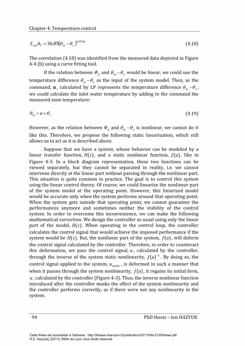
Chapter 4. Temperature control
94 PhD thesis – Ion HAZYUK
( ) 2544.085.36 zinTrad hS θθ −= (4.18)
The correlation (4.18) was identified from the measured data depicted in Figure 4-4 (b) using a curve fitting tool.
If the relation between gΦ and zin θθ − would be linear, we could use the temperature difference zin θθ − as the input of the system model. Then, as the command, u , calculated by LP represents the temperature difference zin θθ − , we could calculate the inlet water temperature by adding to the command the measured zone temperature:
zin u θθ += (4.19)
However, as the relation between gΦ and zin θθ − is nonlinear, we cannot do it like this. Therefore, we propose the following static linearization, which still allows us to act as it is described above.
Suppose that we have a system, whose behavior can be modeled by a linear transfer function, )(sH , and a static nonlinear function, )(uf , like in Figure 4-3. In a block diagram representation, these two functions can be viewed separately, but they cannot be separated in reality, i.e. we cannot intervene directly at the linear part without passing through the nonlinear part. This situation is quite common in practice. The goal is to control this system using the linear control theory. Of course, we could linearize the nonlinear part of the system model at the operating point. However, this liniarized model would be accurate only when the system performs around that operating point. When the system gets outside that operating point, we cannot guarantee the performances anymore and sometimes neither the stability of the control system. In order to overcome this inconvenience, we can make the following mathematical correction. We design the controller as usual using only the linear part of the model, )(sH . When operating in the control loop, the controller calculates the control signal that would achieve the imposed performance if the system would be )(sH . But, the nonlinear part of the system, )(uf , will deform the control signal calculated by the controller. Therefore, in order to counteract this deformation, we pass the control signal, u , calculated by the controller, through the inverse of the system static nonlinearity, 1)( −uf . By doing so, the control signal applied to the system, .nonlinu , is deformed in such a manner that when it passes through the system nonlinearity, )(uf , it regains its initial form, u , calculated by the controller (Figure 4-3). Thus, the inverse nonlinear function introduced after the controller masks the effect of the system nonlinearity and the controller performs correctly, as if there were not any nonlinearity in the system.
Cette thèse est accessible à l'adresse : http://theses.insa-lyon.fr/publication/2011ISAL0130/these.pdf © [I. Hazyuk], [2011], INSA de Lyon, tous droits réservés
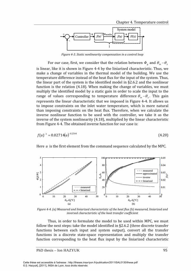
Chapter 4. Temperature control
PhD thesis – Ion HAZYUK 95
Figure 4-3. Static nonlinearity compensation in a control loop
For our case, first, we consider that the relation between gΦ and zin θθ − is linear, like it is shown in Figure 4-4 by the liniarized characteristic. Thus, we make a change of variables in the thermal model of the building. We use the temperature difference instead of the heat flux for the input of the system. Thus, the linear part of the system is the identified model in §2.6.2 and the nonlinear function is the relation (4.18). When making the change of variables, we must multiply the identified model by a static gain in order to scale the input to the range of values corresponding to temperature difference zin θθ − . This gain represents the linear characteristic that we imposed in Figure 4-4. It allows us to impose constraints on the inlet water temperature, which is more natural than imposing constraints on the heat flux. Therefore, when we calculate the inverse nonlinear function to be used with the controller, we take it as the inverse of the system nonlinearity (4.18), multiplied by the linear characteristic from Figure 4-4. The obtained inverse function for our case is:
( ) 2544.01 02714.0)( −− = uuf (4.20)
Here u is the first element from the command sequence calculated by the MPC.
Figure 4-4. (a) Measured and liniarized characteristic of the heat flux (b) measured, liniarized and
inversed characteristic of the heat transfer coefficient
Thus, in order to formulate the model to be used within MPC, we must follow the next steps: take the model identified in §2.6.2 (three discrete transfer functions between each input and system output), convert all the transfer functions in a discrete state-space representation and multiply the transfer function corresponding to the heat flux input by the liniarized characteristic
Cette thèse est accessible à l'adresse : http://theses.insa-lyon.fr/publication/2011ISAL0130/these.pdf © [I. Hazyuk], [2011], INSA de Lyon, tous droits réservés
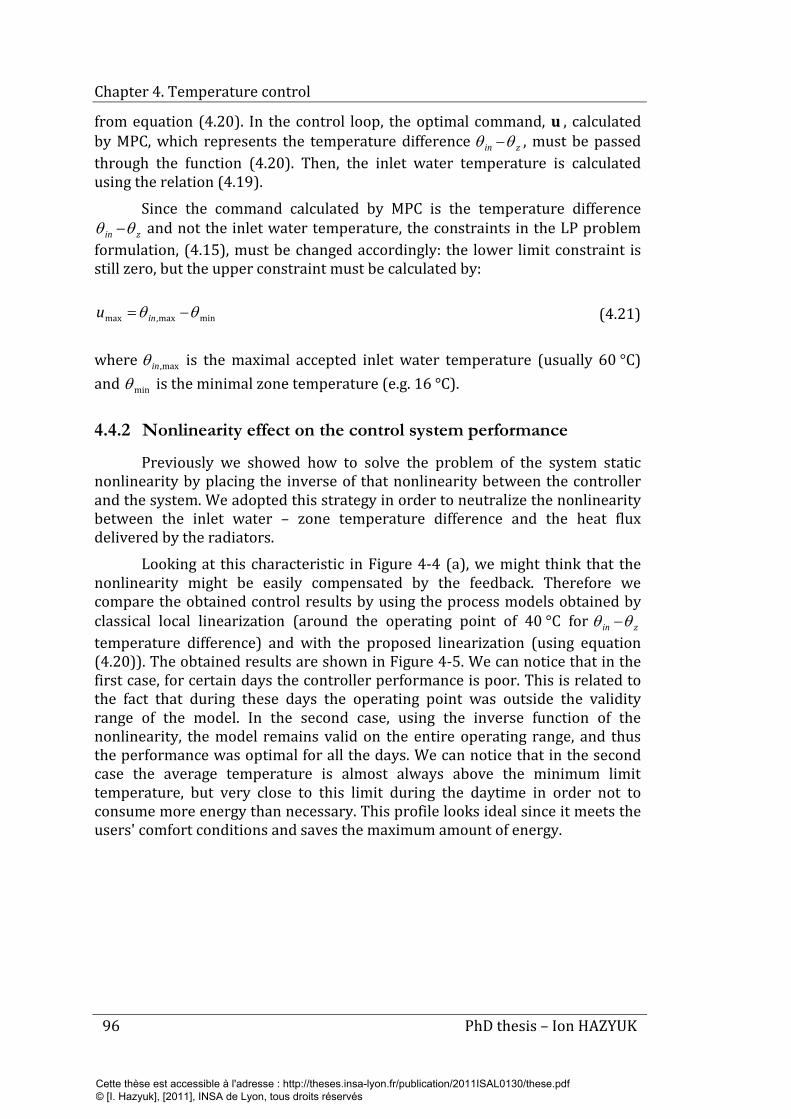
Chapter 4. Temperature control
96 PhD thesis – Ion HAZYUK
from equation (4.20). In the control loop, the optimal command, u , calculated by MPC, which represents the temperature difference zin θθ − , must be passed through the function (4.20). Then, the inlet water temperature is calculated using the relation (4.19).
Since the command calculated by MPC is the temperature difference zin θθ − and not the inlet water temperature, the constraints in the LP problem
formulation, (4.15), must be changed accordingly: the lower limit constraint is still zero, but the upper constraint must be calculated by:
minmax,max θθ −= inu (4.21)
where max,inθ is the maximal accepted inlet water temperature (usually 60 °C) and minθ is the minimal zone temperature (e.g. 16 °C).
4.4.2 Nonlinearity effect on the control system performance
Previously we showed how to solve the problem of the system static nonlinearity by placing the inverse of that nonlinearity between the controller and the system. We adopted this strategy in order to neutralize the nonlinearity between the inlet water – zone temperature difference and the heat flux delivered by the radiators.
Looking at this characteristic in Figure 4-4 (a), we might think that the nonlinearity might be easily compensated by the feedback. Therefore we compare the obtained control results by using the process models obtained by classical local linearization (around the operating point of 40 °C for zin θθ − temperature difference) and with the proposed linearization (using equation (4.20)). The obtained results are shown in Figure 4-5. We can notice that in the first case, for certain days the controller performance is poor. This is related to the fact that during these days the operating point was outside the validity range of the model. In the second case, using the inverse function of the nonlinearity, the model remains valid on the entire operating range, and thus the performance was optimal for all the days. We can notice that in the second case the average temperature is almost always above the minimum limit temperature, but very close to this limit during the daytime in order not to consume more energy than necessary. This profile looks ideal since it meets the users' comfort conditions and saves the maximum amount of energy.
Cette thèse est accessible à l'adresse : http://theses.insa-lyon.fr/publication/2011ISAL0130/these.pdf © [I. Hazyuk], [2011], INSA de Lyon, tous droits réservés
Chapter 4. Temperature control
PhD thesis – Ion HAZYUK 97
Figure 4-5. Simulation results obtained with classical and proposed linearization
4.5 Conclusions
This chapter provides a solution for optimal thermal control of intermittently heated buildings. A comfortable environment influences the user health, satisfaction and productivity. An uncomfortable environment leads to unnecessary energy wasting that would be avoided by assuring a proper comfort. The comfort is mostly affected by the operative temperature. However, usually it is more convenient to measure the indoor temperature instead of operative temperature. Since the comfort standards state that a comfortable ambiance is rather a comfort zone instead of a particular thermal environment, we chose to maintain the temperature within a defined range instead of a certain set-point. As we treat only heating, we defined only the lower temperature bound to be assured. This means that the indoor temperature must be maintained above this bound with lowest energy consumption (which limits in fact the upper comfort temperature level).
Currently, temperature control is done mostly by central room thermostats and/or thermostatic valves on radiators. In the best case, we can find PID controllers on the radiator valve. These strategies cannot guarantee minimal energy consumption because they are not designed for this purpose.
MPC was identified as being one of the best candidates for this task due to its advantages over other control algorithms:
• the ability to use the occupancy schedule and weather forecast for optimal temperature control;
• the possibility to integrate both comfort and energetic criteria in the optimization;
• the ability to handle implicitly the constraints on the system and to operate with multi-input multi-output systems, which is very convenient in building thermal control.
Cette thèse est accessible à l'adresse : http://theses.insa-lyon.fr/publication/2011ISAL0130/these.pdf © [I. Hazyuk], [2011], INSA de Lyon, tous droits réservés
Chapter 4. Temperature control
98 PhD thesis – Ion HAZYUK
MPC acts in two steps: it calculates the command sequence which would optimize the output during a future time horizon and then applies the first value of this sequence to the system. Then, at the next time step, it recalculates the command sequence from the new state of the system. However, the square of the command increment from the classical formulation of the cost function used by MPC is inadequately formulated for the required performances in buildings. First, it does not minimize the energy consumption and second, the use of a trade-off between energy savings and discomfort is subjective. Therefore, in order to overcome these inconveniences we proposed a new formulation of the cost function which minimizes the absolute value of the command.
The principle of the trade-off between energy savings and comfort was also identified as a problem of the current practice in MPC. The drawback is that we can get different performance of the control system depending on what has been privileged – energy savings or comfort. Moreover, there is an additional parameter to be tuned when using trade-off. The problem was solved by changing the principle; we impose the minimal comfort as the lower limit in the optimization algorithm. Thus, MPC calculates a command that assures minimal comfort while using the smallest amount of energy.
By changing the cost function, we were forced to change also the algorithm used to solve the optimization problem. For the cost function we introduced, the proposed solving algorithm is linear programming (LP). Therefore, we formulated the problem so that it fits into the canonical formulation of LP.
The use of MPC requires a dynamical model of the building. During the modeling, we revealed some nonlinearity in the static characteristic of the model. We used this nonlinear characteristic here, in this chapter, for model linearization. This linearization allowed us to use the model on the entire operating range and not just around some operating point, like in classical linearization.
As the nonlinear characteristic between the heat flux and zin θθ − temperature difference seemed not to be so nonlinear, one might believe that the controller in the closed loop can handle very well this situation, eventually poorly degrading the performance. In order to prove the contrary, we provided a simulation example where we compared the results obtained in two situations. In the first situation, we used a local linearized model, while in the second situation, we used the inverse nonlinearity between the controller and the process. The results showed that in the first case, for certain days the control system achieved very low performance, while in the second case, the performance was optimal for every day. Thus, by using the inverse nonlinearity between the controller and the process, we can guarantee the performance on the entire temperature range. On the contrary, we cannot have this certainty if we use just the model linearized around some operating point. For our case, this is very important because, unlike other processes, the buildings operate on the entire temperature range, i.e. the zin θθ − temperature difference always varies between around 0 and 44 °C, and not just around some specific point.
Cette thèse est accessible à l'adresse : http://theses.insa-lyon.fr/publication/2011ISAL0130/these.pdf © [I. Hazyuk], [2011], INSA de Lyon, tous droits réservés
Chapter 4. Temperature control
PhD thesis – Ion HAZYUK 99
Concerning the overall performance, we have shown that MPC has been able to achieve the expected results. The average temperature almost always has been above the minimum comfort temperature, but still very close to this limit during the daytime in order not to consume more energy than necessary.
Although we obtained promising results, advancements in the following directions can be made:
• Here, the thermal control is based on a mono-zone model, even if the tests were performed on a building with several rooms. It would be necessary to investigate multi-zone models. This change will raise many questions: do we develop a MPC by zone or a new distribution function of the heat flux in each zone; how the inter-zone coupling affects the performance; should we define an objective function by zone which takes into account the needs of the adiacent zones? Some investigations in this direction can be found in Morosan et al. (2010).
• In our simulations, we considered that the weather predictions were 100 % reliable. The fact that at each time step the controller re-evaluates the optimization using updated weather forecast fixes the problems but, probably, with a variable performance. Thus, it is necessary to check out weather forecast precision impacts on energy consumption and especially on comfort. Some investigations in this direction can be found in Oldewurtel et al. (2010). Also, as the regulation is based on a mathematical model of the building, it would be very useful a sensitivity analysis of the model parameters’ uncertainties on the control performance.
Cette thèse est accessible à l'adresse : http://theses.insa-lyon.fr/publication/2011ISAL0130/these.pdf © [I. Hazyuk], [2011], INSA de Lyon, tous droits réservés
Chapter 4. Temperature control
100 PhD thesis – Ion HAZYUK
References
ASHRAE (2004). ASHRAE Standard 55-2004: Thermal environmental conditions for human occupancy. Atlanta, GA: American Society of Heating, Refrigerating, and Air-Conditioning Engineers.
Balan, R., Cooper, J., Chao, K.-M., Stan, S. & Donca, R. (2011). Parameter identification and model based predictive control of temperature inside a house. Energy and Buildings, 43(2-3), 748-758.
Bénard, C., Guerrier, B. & Rosset-Louërat, M. M. (1992). Optimal Building Energy Management: Part II---Control. Journal of Solar Energy Engineering, 114, 13-22.
Camacho, E. F. & Bordons, A. C. (2004). Model Predictive Control (2nd ed.). London: Springer-Verlag.
CEN (2005). EN ISO 7730:2005: Ergonomics of the thermal environment - Analytical determination and interpretation of thermal comfort using calculation of the PMV and PPD indices and local thermal comfort criteria. Brussels, Belgium: European Committee for Standardization.
Chen, T. Y. (2001). Real-time predictive supervisory operation of building thermal systems with thermal mass. Energy and Buildings, 33(2), 141-150.
Chen, T. Y. (2002). Application of adaptive predictive control to a floor heating system with a large thermal lag. Energy and Buildings, 34(1), 45-51.
Dounis, A. I. & Caraiscos, C. (2009). Advanced control systems engineering for energy and comfort management in a building environment--A review. Renewable and Sustainable Energy Reviews, 13(6-7), 1246-1261.
Duburcq, S. & Guillerminet, S. (1997). Advanced control for intermittent heating. In: Proceedings of Clima 2000 Conference, August 30 - September 2, 1997, Brussels, Belgium.
Fanger, P. O. (1972). Thermal Comfort Analysis and Application in Environmental Design. New York, NY: McGraw-Hill.
Freire, R. Z., Oliveira, G. H. C. & Mendes, N. (2008). Predictive controllers for thermal comfort optimization and energy savings. Energy and Buildings, 40(7), 1353-1365.
Ghiaus, C. & Hazyuk, I. (2010). Calculation of optimal thermal load of intermittently heated buildings. Energy and Buildings, 42(8), 1248-1258.
Gruber, P., Gwerder, M. & Tödtli, J. (2001). Predictive control for heating applications. In: 7th REHVA World Congress (Clima 2000/Napoli 2001), September 15-18, 2001, Napoli, Italy.
Gyalistras, D. & Gwerder, M. (2010). Use of weather and occupancy forecasts for optimal building climate control (OptiControl): Two years progress
Cette thèse est accessible à l'adresse : http://theses.insa-lyon.fr/publication/2011ISAL0130/these.pdf © [I. Hazyuk], [2011], INSA de Lyon, tous droits réservés
Chapter 4. Temperature control
PhD thesis – Ion HAZYUK 101
report. Zug, Switzerland: Terrestrial Systems Ecology ETH and Building Technologies Division, Siemens Switzerland Ltd.
Gyalistras, D. & The OptiControl Team (2010). Final report: Use of weather and occupancy forecasts for optimal building climate control (OptiControl). Zurich, Switzerland: Terrestrial Systems Ecology ETH.
Karlsson, H. & Hagentoft, C.-E. (2011). Application of model based predictive control for water-based floor heating in low energy residential buildings. Building and Environment, 46(3), 556-569.
Kolokotsa, D., Pouliezos, A., Stavrakakis, G. & Lazos, C. (2009). Predictive control techniques for energy and indoor environmental quality management in buildings. Building and Environment, 44(9), 1850-1863.
Kummert, M., André, P. & Nicolas, J. (1997). Optimised thermal zone controller for integration within a Building Energy Management System. In: Proceedings of CLIMA 2000 conference, August 30 - September 2, 1997, Brussels, Belgium.
Kummert, M., André, P. & Nicolas, J. (2001). Optimal heating control in a passive solar commercial building. Solar Energy, 69(Supplement 6), 103-116.
Lee, K.-h. & Braun, J. E. (2008). Model-based demand-limiting control of building thermal mass. Building and Environment, 43(10), 1633-1646.
Liao, Z., Swainson, M. & Dexter, A. L. (2005). On the control of heating systems in the UK. Building and Environment, 40(3), 343-351.
Ma, Y., Borrelli, F., Hencey, B., Packard, A. & Bortoff, S. (2009). Model predictive control of thermal energy storage in building cooling systems. In: Proceedings of the 48th IEEE Conference on Decision and Control, December 15-18, 2009, Shanghai, China.
Maciejowski, J. M. (2000). Predictive Control with Constraints. London: Prentice Hall.
Meier, A., Aragon, C., Hurwitz, B., Mujumdar, D., Perry, D., Peffer, T., et al. (2010). How people actually use thermostats. In: Proceedings of the 2010 ACEEE Summer Study on Energy Efficiency in Buildings, August 15-20, 2010, Pacific Grove, CA, USA.
Morari, M. & Lee, J. H. (1999). Model predictive control: Past, present and future. Computers & Chemical Engineering, 23(4), 667-682.
Morosan, P.-D., Bourdais, R., Dumur, D. & Buisson, J. (2010). Building temperature regulation using a distributed model predictive control. Energy and Buildings, 42(9), 1445-1452.
Oldewurtel, F., Parisio, A., Jones, C. N., Morari, M., Gyalistras, D., Gwerder, M., et al. (2010). Energy efficient building climate control using Stochastic Model Predictive Control and weather predictions. In: American Control Conference (ACC) 2010, June 30 - July 2, 2010, Baltimore, MD, USA.
Cette thèse est accessible à l'adresse : http://theses.insa-lyon.fr/publication/2011ISAL0130/these.pdf © [I. Hazyuk], [2011], INSA de Lyon, tous droits réservés
Chapter 4. Temperature control
102 PhD thesis – Ion HAZYUK
Paris, B., Eynard, J., Grieu, S., Talbert, T. & Polit, M. (2010). Heating control schemes for energy management in buildings. Energy and Buildings, 42(10), 1908-1917.
Peeters, L., Van der Veken, J., Hens, H., Helsen, L. & D'Haeseleer, W. (2008). Control of heating systems in residential buildings: Current practice. Energy and Buildings, 40(8), 1446-1455.
Prívara, S., Siroký, J., Ferkl, L. & Cigler, J. (2011). Model predictive control of a building heating system: The first experience. Energy and Buildings, 43(2-3), 564-572.
Wang, L. (2009). Model Predictive Control System Design and Implementation using MATLAB. London: Springer-Verlag.
Yuan, S. & Perez, R. (2006). Multiple-zone ventilation and temperature control of a single-duct VAV system using model predictive strategy. Energy and Buildings, 38(10), 1248-1261.
Zhao, H. & Visier, J. C. (1991). Intermittent heating system control based on the quadratic optimization principle. In: Building Simulation, August 20-22, 1991, Nice, France.
Cette thèse est accessible à l'adresse : http://theses.insa-lyon.fr/publication/2011ISAL0130/these.pdf © [I. Hazyuk], [2011], INSA de Lyon, tous droits réservés
103
Chapter 5
Performance assessment
Usually, when temperature controllers are tested, it is considered that the needed energy is always available. Thus, the resulted performances are ideal for the tested controller. However, in reality, the controller acts like a valve: it regulates the energy flow between the minimal value technologically possible and the maximum available energy. If the calculated command is outside this range, it enters in saturation and the obtained performance is degraded. Therefore, in order to obtain realistic performances during the test, we integrated the Model Predictive Control (MPC) algorithm for temperature control of the buildings in a Building Energy Management System (BEMS) and tested by emulation, on a dedicated test bench, its performance concerning the thermal comfort, energy consumption and system wear and tear. As compared to two PID-based classical solutions, the proposed MPC reduces the discomfort up to 97 %, reduces the energy consumption up to 18 %, and reduces the number of on-off cycles of heat pumps up to 78 % and of auxiliary hydraulic pumps up to 89 %.
5.1 Introduction
In Chapter 4, we designed a Model Predictive Controller (MPC) dedicated to temperature control in buildings. This controller calculates the necessary amount of heat to be introduced into the building in order to assure the minimal imposed temperature with minimal energy consumption. In heating system based on hot water, the energy flux of the radiators is manipulated by varying either the inlet water temperature or the water flow. The MPC proposed in Chapter 4 calculates the inlet water temperature considering a constant flow through radiators.
In Chapter 4, we have considered that the energy source can deliver the requested power when necessary, i.e. the hot water is at the temperature
Cette thèse est accessible à l'adresse : http://theses.insa-lyon.fr/publication/2011ISAL0130/these.pdf © [I. Hazyuk], [2011], INSA de Lyon, tous droits réservés
Chapter 5. Performance assessment
104 PhD thesis – Ion HAZYUK
demanded by the controller. The controller acts by reducing the flow of energy from the maximum available down to the technological achievable minima. When thermal energy is provided by a hydraulic heating system, a fully functional controller must handle the mass flow in the system. The difficulty is that the hydraulic heating systems are multipurpose systems, i.e. they are used for building heating but also for Domestic Hot Water (DHW) preparation. The coexistence in the same building of renewable and conventional energy sources transforms the heating hydraulic systems into multisource systems. The MPC proposed in Chapter 4 needs to be integrated in the Building Energy Management Systems (BEMS) of this multi-source multi-consumer system.
BEMS are designed to provide comfort in buildings, to reduce energy consumption but also to manage wisely the hydraulic system itself. The hydraulic system used for our test building contains equipments like valves, hydraulic pumps and a heat pump. The command of most of them is on-off, which wears them if they are frequently switched. This is even more critical in the case of very expensive equipments like the heat pumps. Therefore, an important characteristic we must look at in a BEMS is the number of on-off cycles of the hydraulic heating equipment.
The first point treated in this chapter is the design of a BEMS which integrates the MPC designed in Chapter 4. We present the hydraulic heating system itself and the way to operate it in order to assure hot water and comfortable thermal environment with minimal energy consumption and reduced solicitation of the hydraulic equipment.
The second point treated in this chapter is the test and evaluation of the proposed BEMS against two classical solutions based on PID and scheduled start PID controllers. In order to have reproducible test conditions, we have chosen to test the proposed BEMS through emulation. We implemented the control algorithm on an industrial microcomputer and tested this controller on the test bench for building controllers of CSTB (French Scientific and Technical Construction Center).
The assessment of the proposed BEMS performance is made against several criteria concerning thermal comfort, energy consumption and number of on-off cycles. The results of these indices are then compared with those of the classical solutions in order to determine the benefits of the proposed control algorithm.
5.2 Hydraulic system specification
The analyzed hydronic heating system uses a combination of classical and renewable sources for indoor climate control and for domestic hot water (DHW) preparation (Figure 5-1). Since it has two kind of energy sources (classical and renewable) and two kind of consumers (building heating and DHW preparation), it is a multi-source multi-consumer system.
Cette thèse est accessible à l'adresse : http://theses.insa-lyon.fr/publication/2011ISAL0130/these.pdf © [I. Hazyuk], [2011], INSA de Lyon, tous droits réservés
Chapter 5. Performance assessment
PhD thesis – Ion HAZYUK 105
The hydraulic system from Figure 5-1 has the following main components:
• Two renewable energy sources, i.e. a solar panel of 20 m2 (point 1) and an air-water heat pump (point 7) and a classical energy source, i.e. a 2 kW electrical heater (point 8). The heat pump supplies water at 65 °C, independent of the outdoor temperature.
• Two energy consumers, hot water consumption (point 16) and water radiators for building heating (point 19). Each room contains a radiator.
• Two hot water storage tanks. The first one (point 4) having 300 liters is coupled to the solar panel and the second one (point 10) having 100 liters is dedicated to DHW preparation. Both tanks are well insulated and placed in a heated space. The electrical heater is placed in the upper part of the DHW tank.
• A hydraulic decoupling bottle (point 15) which creates a neutral hydraulic point between the primary and secondary circuits in order to avoid any interactive dynamic pressure induced by their pumps (Ghoul, 1999).
The solar panel (point 1) heats the water from the first storage tank (point 4) through the heat exchanger (point 6) placed at the bottom of the tank. The water between the solar panel and the tank is circulated by a pump (point 2) through a 3-way valve (point 3).
The second storage tank (point 10) is dedicated exclusively for DHW preparation. The water from this tank can be heated in three different ways. First possibility is to heat it using the hot water from the solar tank (point 4). The pump (point 11) can circulate the water between these two tanks thus replacing the water from the DHW tank by the hot water from the solar storage tank. The second possibility is to heat DHW by the heat pump (point 7) through the heat exchanger from the bottom of the tank (point 9). The heat pump supplies hot water at 65 °C which is circulated by the pump (point 13) through the 3-way valve (point 12) directly to the heat exchanger (point 9). The third possibility to heat the DHW is to use the electrical heater (point 8) integrated in the upper part of the DHW tank (point 10).
In each room of the building there is a water radiator (points 19); its hot water can be supplied by two sources: the heat pump (point 7) and the solar storage tank (point 4). A decoupling bottle (point 15) separates the consumer hydraulic circuit, to which the radiators are linked, from the supply circuits. Every time the building is heated, at least two pumps will operate simultaneously: the pump of the consumer circuit (point 18) and one of the pumps of the supply circuits: either the pump (point 14) circulating water between the decoupling bottle and the heat exchanger (point 5) from the solar tank or the pump (point 13) that circulates water from the heating pump to the decoupling bottle through the 3-way valve (point 12). The water temperature
Cette thèse est accessible à l'adresse : http://theses.insa-lyon.fr/publication/2011ISAL0130/these.pdf © [I. Hazyuk], [2011], INSA de Lyon, tous droits réservés
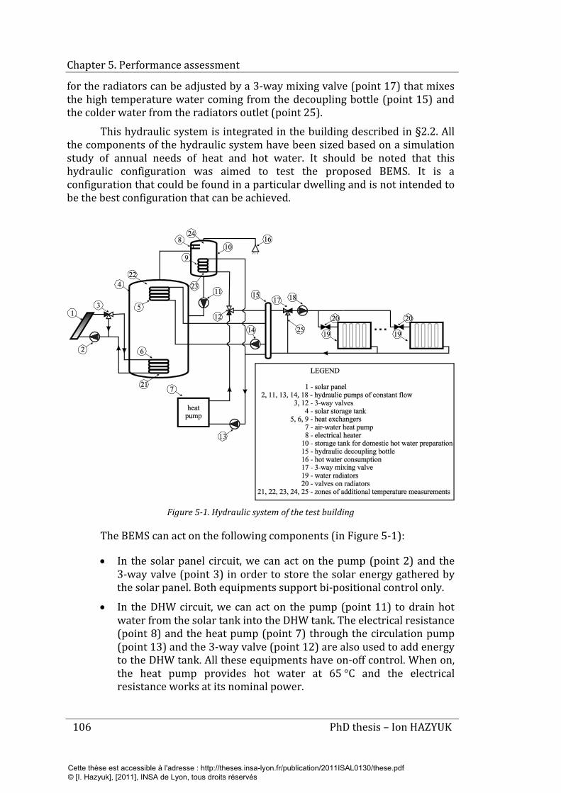
Chapter 5. Performance assessment
106 PhD thesis – Ion HAZYUK
for the radiators can be adjusted by a 3-way mixing valve (point 17) that mixes the high temperature water coming from the decoupling bottle (point 15) and the colder water from the radiators outlet (point 25).
This hydraulic system is integrated in the building described in §2.2. All the components of the hydraulic system have been sized based on a simulation study of annual needs of heat and hot water. It should be noted that this hydraulic configuration was aimed to test the proposed BEMS. It is a configuration that could be found in a particular dwelling and is not intended to be the best configuration that can be achieved.
Figure 5-1. Hydraulic system of the test building
The BEMS can act on the following components (in Figure 5-1):
• In the solar panel circuit, we can act on the pump (point 2) and the 3-way valve (point 3) in order to store the solar energy gathered by the solar panel. Both equipments support bi-positional control only.
• In the DHW circuit, we can act on the pump (point 11) to drain hot water from the solar tank into the DHW tank. The electrical resistance (point 8) and the heat pump (point 7) through the circulation pump (point 13) and the 3-way valve (point 12) are also used to add energy to the DHW tank. All these equipments have on-off control. When on, the heat pump provides hot water at 65 °C and the electrical resistance works at its nominal power.
Cette thèse est accessible à l'adresse : http://theses.insa-lyon.fr/publication/2011ISAL0130/these.pdf © [I. Hazyuk], [2011], INSA de Lyon, tous droits réservés
Chapter 5. Performance assessment
PhD thesis – Ion HAZYUK 107
• In the heating distribution circuit, the heating control system can act in two ways. First way is by acting on each radiator valve (points 20) in order to control the water flow traversing the radiators. Second possibility is to control the radiator inlet water temperature by the 3-way mixing valve (point 17) on the consumer hydraulic circuit. In both cases the control can be either bi-positional or continuous. Also, in both cases the controller drains the water acting on the pump (point 18) from the consumer circuit and on the pumps (point 13 or 14) from the source circuits. The heat flux from the heat pump is directed to the radiators by a 3-way valve (point 12). The pumps and the non-mixing 3-way valve support only bi-positional command.
Several constrains on the hydraulic system operation must be taken into account. The solar tank (point 4) and the heat pump (point 7) cannot supply the radiators simultaneously. Since the 3-way valve (point 12) can direct water in a single direction, the heat pump cannot supply simultaneously the radiators and DHW tank (point 10). On the contrary, the solar tank can supply at the same time water to the DHW tank and to the heating system. The DHW tank can be heated by all three sources simultaneously, i.e. solar tank, heat pump and electrical resistance. It must be reminded that all the hydraulic pumps are constant flow pumps.
5.3 Reference PID-based building energy management systems
In order to asses the performance of the proposed BEMS, first, we define two reference systems based on PID and PID plus scheduled start controllers, which are among the most advanced systems that can be found today in dwellings (Dounis & Caraiscos, 2009; Liao, Swainson & Dexter, 2005; Peeters, Van der Veken, Hens, Helsen & D'Haeseleer, 2008). The role of the BEMS is to act on every pump and valve of the hydraulic system in order to assure the users comfort, i.e. proper indoor temperature and hot water, while using less possible energy. As stated in §4.2.1, proper indoor temperature means that the indoor air temperature must be above a minimal limit, which is defined by the users. In our case, the minimal temperature was set to 19 °C for the daytime, i.e. between 07:00am and 10:00pm, and 16 °C for the nighttime, i.e. between 10:00pm and 07:00am.
5.3.1 First reference control system
The PID-base BEMS is described in Figure 5-2 by GRAFCET, which is a standardized language for discrete event processes (David & Alla, 1992).
Cette thèse est accessible à l'adresse : http://theses.insa-lyon.fr/publication/2011ISAL0130/these.pdf © [I. Hazyuk], [2011], INSA de Lyon, tous droits réservés
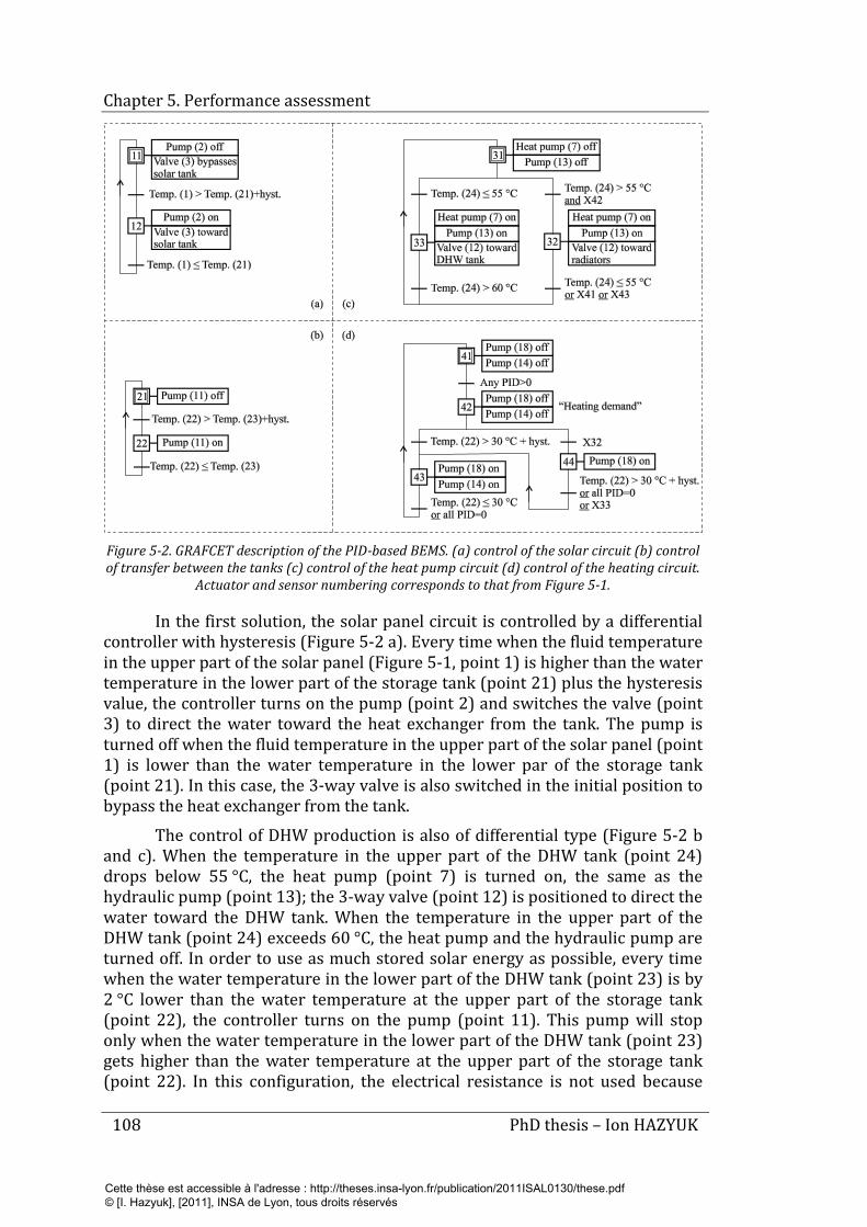
Chapter 5. Performance assessment
108 PhD thesis – Ion HAZYUK
Figure 5-2. GRAFCET description of the PID-based BEMS. (a) control of the solar circuit (b) control of transfer between the tanks (c) control of the heat pump circuit (d) control of the heating circuit.
Actuator and sensor numbering corresponds to that from Figure 5-1.
In the first solution, the solar panel circuit is controlled by a differential controller with hysteresis (Figure 5-2 a). Every time when the fluid temperature in the upper part of the solar panel (Figure 5-1, point 1) is higher than the water temperature in the lower part of the storage tank (point 21) plus the hysteresis value, the controller turns on the pump (point 2) and switches the valve (point 3) to direct the water toward the heat exchanger from the tank. The pump is turned off when the fluid temperature in the upper part of the solar panel (point 1) is lower than the water temperature in the lower par of the storage tank (point 21). In this case, the 3-way valve is also switched in the initial position to bypass the heat exchanger from the tank.
The control of DHW production is also of differential type (Figure 5-2 b and c). When the temperature in the upper part of the DHW tank (point 24) drops below 55 °C, the heat pump (point 7) is turned on, the same as the hydraulic pump (point 13); the 3-way valve (point 12) is positioned to direct the water toward the DHW tank. When the temperature in the upper part of the DHW tank (point 24) exceeds 60 °C, the heat pump and the hydraulic pump are turned off. In order to use as much stored solar energy as possible, every time when the water temperature in the lower part of the DHW tank (point 23) is by 2 °C lower than the water temperature at the upper part of the storage tank (point 22), the controller turns on the pump (point 11). This pump will stop only when the water temperature in the lower part of the DHW tank (point 23) gets higher than the water temperature at the upper part of the storage tank (point 22). In this configuration, the electrical resistance is not used because
Cette thèse est accessible à l'adresse : http://theses.insa-lyon.fr/publication/2011ISAL0130/these.pdf © [I. Hazyuk], [2011], INSA de Lyon, tous droits réservés
Chapter 5. Performance assessment
PhD thesis – Ion HAZYUK 109
DHW preparation is the priority task for the heat pump, which is able to assure anytime the availability of DHW.
For the thermal environment control, a PID controller is used on each radiator valve (points 20). Thus, the valve positions are controlled continuously between wide opened and closed positions and the effect is a varying flow rate through the radiators. The input of the PID controller is the error between the indoor set-point temperature and the air temperature of the room, which is given by a temperature sensor from the concerned room. The set-point temperature considered for PID controller will be the minimal temperature limit given above, i.e. 19 °C between 07:00am and 10:00pm, and 16 °C between 10:00pm and 07:00am. The controller output is the position of the valve on the radiator. The controller parameters were tuned using Ziegler-Nichols method (Ziegler & Nichols, 1942), and for our test building they are: 2=P and sI 1600= ; the derivative component is not used, thus 0=D . If at least one of the PID controllers gives a nonzero command, i.e. a valve is being opened, the management system starts up the pump of the consumer circuit (point 18). The 3-way mixing valve (point 17) is always positioned to drain hot water from the decoupling bottle. When there is a demand for heating, the solar storage tank is the priority hot water supplier (Figure 5-2 d). If the water temperature in the upper part of the storage tank (point 22) is higher than 30 °C, water is drained from the tank by turning on the pump (point 14). If the water temperature in the upper part of the storage tank (point 22) is lower than 30 °C, we check if the heat pump is not used for DHW preparation. If it is not used, we turn on the heat pump (point 7) and the hydraulic pump (point 13) in order to supply hot water for the heating (Figure 5-2 c). But, if the heat pump is already used and the water in the upper part of the storage tank is lower than 30 °C, we cut down the pump (point 18) of the consumer circuit and wait until one of the sources will be available.
We can notice that this configuration gives a higher priority to DHW preparation then to building heating. In the simulation tests, we realized over a year, we practically never had intervals where there was a heating demand and both sources were not available. Yet, it does not mean that we are exempted of this situations for other occupation scenarios or/and meteorological conditions.
5.3.2 Second reference control system
The second configuration of the BEMS is very similar to the first one. The only difference between these two is the PID controller for the valves on radiators. As stated before, the indoor set-point temperature changes form 16 to 19 °C at 07:00am and from 19 to 16 °C at 10:00pm. Also, in order to assure the comfort, it is required to maintain the indoor air mean temperature above the minimal limit. A PID controller, like the one used in the first BEMS configuration, can not satisfy this requirement. The set-point will change at 07:00am and only then the controller will open up the valves on the radiators. Thus, due to the thermal inertia, the indoor temperature will not reach immediately 19 °C so the comfort will be compromised at the beginning of the daytime.
Cette thèse est accessible à l'adresse : http://theses.insa-lyon.fr/publication/2011ISAL0130/these.pdf © [I. Hazyuk], [2011], INSA de Lyon, tous droits réservés

Chapter 5. Performance assessment
110 PhD thesis – Ion HAZYUK
A solution to this problem is implemented in the second reference BEMS. Practically, we keep the same PID controller on the terminal valves, with the same parameters of the controller, and shift two hours ahead the set-point change moment in the morning. Now the set-point will change at 05:00am instead of 07:00am and this set-back time allows the increasing of the indoor temperature. This technique is also called PID with scheduled start. The period of two hours ahead was obtained from trial and error by searching the maximum time for heating up the building in winter period. By using a PID with scheduled start instead of a simple PID controller, we will get better comfort. However, because the PID with scheduled start will start earlier, the building will consume more energy.
5.4 Proposed MPC-based building energy management system
The thermal control part of the proposed BEMS is principally based on the MPC controller that is described in Chapter 4. The control strategy of the sources (Figure 5-3) resembles that of the reference BEMS: it is also based on differential control. Thus, the solar panel circuit is controlled by a differential controller with hysteresis (Figure 5-3 a), exactly as in the reference BEMS. The hydraulic pump starts up when the fluid temperature in the upper part of the solar panel is higher than the water temperature in the lower part of the storage tank and stops down when this condition is no more satisfied. In order to avoid frequent pump switching, a hysteresis is used.
The control of domestic hot water (DHW) production is also of differential type but slightly different from that of the reference configuration. Here, also as in the reference configuration, the solar storage tank and the heat pump are used for DHW preparation. However, if in the reference case the heat pump priority was to prepare DHW, in this case the priority of the heat pump is the building heating. Therefore, in order to assure at any time the availability of the hot water, we use an electrical resistance dedicated uniquely for hot water preparation. This resistance is placed in the upper part of the DHW tank so it heats almost instantly the water for use. Thus, the control strategy for the DHW preparation is the following: when the temperature in the upper part of the DHW tank drops below 55 °C and the heat pump is not used for building heating at that moment, the control system will turn on the heat pump and the hydraulic pump (Figure 5-1, points 7 and 13) and position the 3-way valve (point 12) to direct the water toward the DHW tank. When the temperature in the upper part of the DHW tank (point 24) exceeds 60 °C, the heat pump and the hydraulic pump are turned off (Figure 5-3 c). If the heat pump is not available, then we turn on the electrical resistance (point 8) at nominal power (Figure 5-3 e).
Cette thèse est accessible à l'adresse : http://theses.insa-lyon.fr/publication/2011ISAL0130/these.pdf © [I. Hazyuk], [2011], INSA de Lyon, tous droits réservés
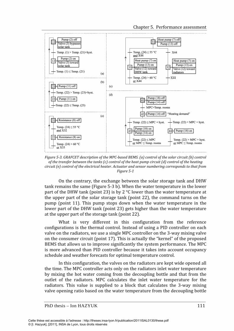
Chapter 5. Performance assessment
PhD thesis – Ion HAZYUK 111
Figure 5-3. GRAFCET description of the MPC-based BEMS. (a) control of the solar circuit (b) control
of the transfer between the tanks (c) control of the heat pump circuit (d) control of the heating circuit (e) control of the electrical heater. Actuator and sensor numbering corresponds to that from
Figure 5-1
On the contrary, the exchange between the solar storage tank and DHW tank remains the same (Figure 5-3 b). When the water temperature in the lower part of the DHW tank (point 23) is by 2 °C lower than the water temperature at the upper part of the solar storage tank (point 22), the command turns on the pump (point 11). This pump stops down when the water temperature in the lower part of the DHW tank (point 23) gets higher than the water temperature at the upper part of the storage tank (point 22).
What is very different in this configuration from the reference configurations is the thermal control. Instead of using a PID controller on each valve on the radiators, we use a single MPC controller on the 3-way mixing valve on the consumer circuit (point 17). This is actually the “kernel” of the proposed BEMS that allows us to improve significantly the system performance. The MPC is more advanced than PID controller because it takes into account occupancy schedule and weather forecasts for optimal temperature control.
In this configuration, the valves on the radiators are kept wide opened all the time. The MPC controller acts only on the radiators inlet water temperature by mixing the hot water coming from the decoupling bottle and that from the outlet of the radiators. MPC calculates the inlet water temperature for the radiators. This value is supplied to a block that calculates the 3-way mixing valve opening ratio based on the water temperature from the decoupling bottle
Cette thèse est accessible à l'adresse : http://theses.insa-lyon.fr/publication/2011ISAL0130/these.pdf © [I. Hazyuk], [2011], INSA de Lyon, tous droits réservés
Chapter 5. Performance assessment
112 PhD thesis – Ion HAZYUK
(point 15) and radiators outlet water temperature (point 25) measurements. The 3-way mixing valve opening ratio is calculated by:
coldhot
MPChot
TTTT
r−−
= (5.1)
where:
r is the 3-way mixing valve opening ratio (zero corresponds to completely pass the hot water from the decoupling bottle and one corresponds to inject the outlet water again into radiators)
hotT – water temperature from the decoupling bottle (point 15)
coldT – water temperature of the outlet water (point 25)
MPCT – water temperature calculated by MPC.
The opening rate of the 3-way mixing valve must vary between zero and one. Therefore, in order to relation (5.1) be valid, the following constraint must be imposed:
MPChot TT ≥ (5.2)
When there is a demand for heating from MPC, the controller will automatically start the pump (point 18) of the consumer circuit (Figure 5-3 d). The solar storage tank has priority for hot water supplier for the heating. First, we check if the water temperature of the upper part in the tank (point 22) satisfies the condition (5.2), where hotT is the water temperature of the upper part of the solar tank. If the condition (5.2) is satisfied, than the controller starts the hydraulic pump (point 14), and if not, the controller automatically starts the heat pump and the affiliated hydraulic pump (points 7 and 13) and turn the 3-way valve (point 12) toward the decoupling bottle (Figure 5-3 b). When the heating controller decides to use the heat pump for indoor heating, the 3-way valve (point 12) will always be switched toward the decoupling bottle because heating is the priority task of the heat pump. So if the heat pump is in the middle of the DHW preparation, this action will be interrupted and the task is taken by the electrical resistance (point 8). Also when the building is heated by the heat pump, the constraint (5.2) will always be satisfied because the heat pump provides always water at 65 °C and we set a constraint in MPC for the maximal command, i.e. inlet water temperature, to 60 °C. Thus, the water temperature supplied by the heat pump will always be higher than that demanded by the MPC.
Cette thèse est accessible à l'adresse : http://theses.insa-lyon.fr/publication/2011ISAL0130/these.pdf © [I. Hazyuk], [2011], INSA de Lyon, tous droits réservés
Chapter 5. Performance assessment
PhD thesis – Ion HAZYUK 113
5.5 Control performance criteria
In order to asses the performance of the proposed BEMS, we compare the obtained control results with those of two reference systems. In order to do this, we need to have performance criteria calculated for the entire test period. These criteria must reflect in a single value the specific performance we are looking for. Hereafter we present the performances that we are interested in and the criteria that are usually used to reflect these performances.
As the aim of the BEMS is to assure the thermal comfort with minimal energy consumption, the performances we are looking for are the respect of the required comfort condition and the consumed energy. A particular feature of a control system is the aggressiveness of the calculated command. This feature plays a decisive role for the wear and tear of the actuators, so it becomes important in situations where we have expensive actuators like here, i.e. heat and hydraulic pumps.
5.5.1 Comfort criteria
As the system we treat is a multi-source multi-consumer and we have two consumers, i.e. building heating and DHW preparation, the comfort is related to both tasks. For DHW preparation, the comfort is considered as being assured if the water temperature at the upper part of the DHW tank is always higher than 55 °C. This will prevent the development of the Legionella.
For the thermal comfort, in §5.3 we defined the lower limit temperature of 19 °C between 07:00am and 10:00pm, and 16 °C between 10:00pm and 07:00am (CSTB, 2005). Thus, the comfort is assured if the indoor air temperature is always above this minimal limit. Here, we will use two criteria: one concerning only the thermal comfort, which is the excess-weighted PPD, and one concerning a combination between comfort and energy consumption, which is optimal start of the heating system. These criteria are described hereafter.
5.5.1.1 Excess-weighted PPD (PPD.h)
Fanger (1972) developed Predictive Mean Vote (PMV) and Predicted Percentage of Dissatisfied people (PPD) indices, which are used by numerous national and international regulations, and especially by the international norm ISO 7730 (CEN, 2005). Yet, PMV and PPD are indices describing the instantaneous comfort, while we need a criterion to appreciate the thermal comfort on the entire test period. Therefore, in our comparisons we use the excess-weighted PPD which is described in the European norm EN 15251 (CEN, 2007) and applied in the following.
Lets consider that the comfort zone (i.e. the temperature domain in which the comfort is satisfied) corresponds to a PMV index that varies between -0.5 and +0.5 (category 2 in EN 15121), which corresponds to the minimal temperature limit and to the maximal one, respectively. A minimal energy
Cette thèse est accessible à l'adresse : http://theses.insa-lyon.fr/publication/2011ISAL0130/these.pdf © [I. Hazyuk], [2011], INSA de Lyon, tous droits réservés
Chapter 5. Performance assessment
114 PhD thesis – Ion HAZYUK
strategy will always result in maintaining the zone temperature at the lower limit of the comfort temperature range. Therefore, the upper limit of the temperature is automatically implemented by the use of this strategy. This is why we do not consider de upper limit of temperature for discomfort evaluation.
It is defined a weighting function, wf , for the time while the PMV exceeds the comfort zone, which is a function of PPD. This weighting function is zero when the PMV is above the inferior limit:
5.0,0 −>= PMVwhenwf (5.3)
and is calculated by the following relation when PMV is below the inferior limit:
5.0,min
−<= PMVwhenPPD
PPDwf (5.4)
where minPPD is the PPD corresponding to 5.0−=PMV , that is %10min =PPD . Once we get the distribution of the weighting function, we calculate the excess-weighted PPD by summing up the values of the weighting function multiplied by the time interval for which we had each particular value of the weighting function:
∑=
⋅=n
iwfi i
twfhPPD1
. (5.5)
where n is the number of distinct weighting function values and iwft is the time
interval for which we had the ith value of the weighting function. Thus, we have an evaluation of the people dissatisfaction over a time period, integrated in a single value representation. In our case, we calculate this index only for the daytime, between 07:00am and 10:00pm, and we did not take into account the nighttime.
5.5.1.2 Optimal start
One of the crucial points of a BEMS is its ability to restart the heating at the right moment in order to recover the building from night setback. The lack of such a functionality leads to either discomfort at the beginning of the daytime period, if the heating is restarted too late, or energy wasted, if the heating is restarted too early. The procedure for the optimal start test is given in the European norm EN 12098-2 (CEN, 2001). The appreciation of a good performance according to the norm is illustrated in Figure 5-4. At the moment when the set-point temperature changes in the morning from 16 °C to 19 °C, we draw a check window around the point corresponding to 07:00am and 19 °C (Figure 5-4). The check window has a width of 30 minutes (15 minutes before
Cette thèse est accessible à l'adresse : http://theses.insa-lyon.fr/publication/2011ISAL0130/these.pdf © [I. Hazyuk], [2011], INSA de Lyon, tous droits réservés
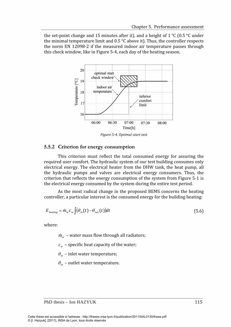
Chapter 5. Performance assessment
PhD thesis – Ion HAZYUK 115
the set-point change and 15 minutes after it), and a height of 1 °C (0.5 °C under the minimal temperature limit and 0.5 °C above it). Thus, the controller respects the norm EN 12098-2 if the measured indoor air temperature passes through this check window, like in Figure 5-4, each day of the heating season.
Figure 5-4. Optimal start test
5.5.2 Criterion for energy consumption
This criterion must reflect the total consumed energy for assuring the required user comfort. The hydraulic system of our test building consumes only electrical energy. The electrical heater from the DHW tank, the heat pump, all the hydraulic pumps and valves are electrical energy consumers. Thus, the criterion that reflects the energy consumption of the system from Figure 5-1 is the electrical energy consumed by the system during the entire test period.
As the most radical change in the proposed BEMS concerns the heating controller, a particular interest is the consumed energy for the building heating:
( )∫ −= dtttcmE outinwwheating )()( θθ (5.6)
where:
wm – water mass flow through all radiators;
wc – specific heat capacity of the water;
inθ – inlet water temperature;
inθ – outlet water temperature.
Cette thèse est accessible à l'adresse : http://theses.insa-lyon.fr/publication/2011ISAL0130/these.pdf © [I. Hazyuk], [2011], INSA de Lyon, tous droits réservés
Chapter 5. Performance assessment
116 PhD thesis – Ion HAZYUK
5.5.3 Number of on-off cycles criteria
The hydraulic system from Figure 5-1 contains some equipment, like hydraulic and heat pumps, which are very sensitive to multiple restart cycles. Therefore, an additional performance that we are looking at is the number of on-off cycles of the hydraulic and heat pumps. A smaller number of restart cycles is considered as a better performance because it reduces the wear and tear of the actuators.
5.6 Testing and comparison of performance
A control system may be tested in different ways:
• Simulation – both the process and the controller are represented by models implemented in the same or in different simulation tools. This option gives reproducible and rapid results because simulation usually takes much less time than real time tests.
• Emulation – the process is represented by its model and the controller is a physical equipment. Since the real controller is tested, the test is done in real time, i.e. one simulation second is equal to one real second. The advantage is that the real controller is tested in reproducible conditions, which allows us to compare the performance of different controllers.
• In-situ – both the process and the controller are real. The test is done in real time. The advantage here is to have all the plant uncertainties that cannot be modeled in the simulation software. But, in this case, the testing is much more expensive and usually it is almost impossible to have reproducible test conditions.
Since we want to compare three different BEMS, the primordial condition is to have reproducible test conditions, while keeping conditions close to real operation.
The building described in §2.2 and the hydraulic system from Figure 5-1 was implemented in Simbad software (Husaunndee, Lahrech, Vaezi-Nejad & Visier, 1997), which is a dedicated building simulation toolbox in Matlab/Simulink developed by the CSTB and used to emulate buildings and systems in order to assess the performance of real controllers.
As the tests were going to be done in real time, it was impossible for us to test all three BEMS for the entire heating season. Therefore we have chosen to run the test for six days periods representative for winter and mid season weather. The choice was motivated by the fact that in winter we have low outdoor temperatures but with low variation amplitudes between two days; in mid season the variation amplitudes between two days are large enough in order to have time periods when the heating system must be turned on and off in the same day. Also, we have chosen to do the tests for two different
Cette thèse est accessible à l'adresse : http://theses.insa-lyon.fr/publication/2011ISAL0130/these.pdf © [I. Hazyuk], [2011], INSA de Lyon, tous droits réservés
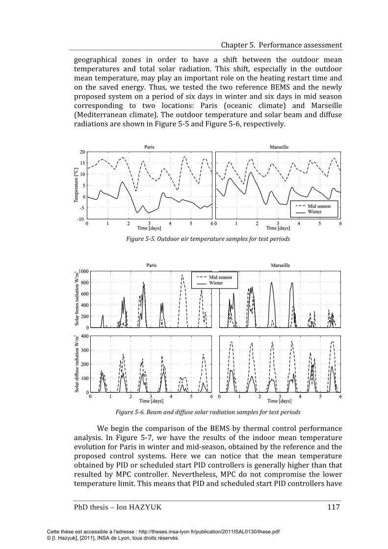
Chapter 5. Performance assessment
PhD thesis – Ion HAZYUK 117
geographical zones in order to have a shift between the outdoor mean temperatures and total solar radiation. This shift, especially in the outdoor mean temperature, may play an important role on the heating restart time and on the saved energy. Thus, we tested the two reference BEMS and the newly proposed system on a period of six days in winter and six days in mid season corresponding to two locations: Paris (oceanic climate) and Marseille (Mediterranean climate). The outdoor temperature and solar beam and diffuse radiations are shown in Figure 5-5 and Figure 5-6, respectively.
Figure 5-5. Outdoor air temperature samples for test periods
Figure 5-6. Beam and diffuse solar radiation samples for test periods
We begin the comparison of the BEMS by thermal control performance analysis. In Figure 5-7, we have the results of the indoor mean temperature evolution for Paris in winter and mid-season, obtained by the reference and the proposed control systems. Here we can notice that the mean temperature obtained by PID or scheduled start PID controllers is generally higher than that resulted by MPC controller. Nevertheless, MPC do not compromise the lower temperature limit. This means that PID and scheduled start PID controllers have
Cette thèse est accessible à l'adresse : http://theses.insa-lyon.fr/publication/2011ISAL0130/these.pdf © [I. Hazyuk], [2011], INSA de Lyon, tous droits réservés
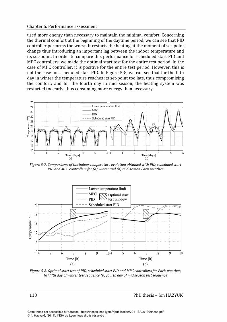
Chapter 5. Performance assessment
118 PhD thesis – Ion HAZYUK
used more energy than necessary to maintain the minimal comfort. Concerning the thermal comfort at the beginning of the daytime period, we can see that PID controller performs the worst. It restarts the heating at the moment of set-point change thus introducing an important lag between the indoor temperature and its set-point. In order to compare this performance for scheduled start PID and MPC controllers, we made the optimal start test for the entire test period. In the case of MPC controller, it is positive for the entire test period. However, this is not the case for scheduled start PID. In Figure 5-8, we can see that for the fifth day in winter the temperature reaches its set-point too late, thus compromising the comfort; and for the fourth day in mid season, the heating system was restarted too early, thus consuming more energy than necessary.
Figure 5-7. Comparisons of the indoor temperature evolution obtained with PID, scheduled start
PID and MPC controllers for (a) winter and (b) mid-season Paris weather
Figure 5-8. Optimal start test of PID, scheduled start PID and MPC controllers for Paris weather;
(a) fifth day of winter test sequence (b) fourth day of mid season test sequence
Cette thèse est accessible à l'adresse : http://theses.insa-lyon.fr/publication/2011ISAL0130/these.pdf © [I. Hazyuk], [2011], INSA de Lyon, tous droits réservés
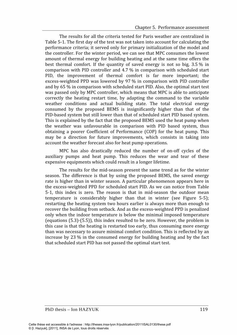
Chapter 5. Performance assessment
PhD thesis – Ion HAZYUK 119
The results for all the criteria tested for Paris weather are centralized in Table 5-1. The first day of the test was not taken into account for calculating the performance criteria; it served only for primary initialization of the model and the controller. For the winter period, we can see that MPC consumes the lowest amount of thermal energy for building heating and at the same time offers the best thermal comfort. If the quantity of saved energy is not so big, 3.5 % in comparison with PID controller and 4.7 % in comparison with scheduled start PID, the improvement of thermal comfort is far more important; the excess-weighted PPD was lowered by 97 % in comparison with PID controller and by 65 % in comparison with scheduled start PID. Also, the optimal start test was passed only by MPC controller, which means that MPC is able to anticipate correctly the heating restart time, by adapting the command to the variable weather conditions and actual building state. The total electrical energy consumed by the proposed BEMS is insignificantly higher than that of the PID-based system but still lower than that of scheduled start PID based system. This is explained by the fact that the proposed BEMS used the heat pump when the weather was unfavourable in comparison with PID based system, thus obtaining a poorer Coefficient of Performance (COP) for the heat pump. This may be a direction for future improvements, which consists in taking into account the weather forecast also for heat pump operations.
MPC has also drastically reduced the number of on-off cycles of the auxiliary pumps and heat pump. This reduces the wear and tear of these expensive equipments which could result in a longer lifetime.
The results for the mid-season present the same trend as for the winter season. The difference is that by using the proposed BEMS, the saved energy rate is higher than in winter season. A particular phenomenon appears here in the excess-weighted PPD for scheduled start PID. As we can notice from Table 5-1, this index is zero. The reason is that in mid-season the outdoor mean temperature is considerably higher than that in winter (see Figure 5-5); restarting the heating system two hours earlier is always more than enough to recover the building from setback. And as the excess-weighted PPD is penalized only when the indoor temperature is below the minimal imposed temperature (equations (5.3)-(5.5)), this index resulted to be zero. However, the problem in this case is that the heating is restarted too early, thus consuming more energy than was necessary to assure minimal comfort condition. This is reflected by an increase by 23 % in the consumed energy for building heating and by the fact that scheduled start PID has not passed the optimal start test.
Cette thèse est accessible à l'adresse : http://theses.insa-lyon.fr/publication/2011ISAL0130/these.pdf © [I. Hazyuk], [2011], INSA de Lyon, tous droits réservés
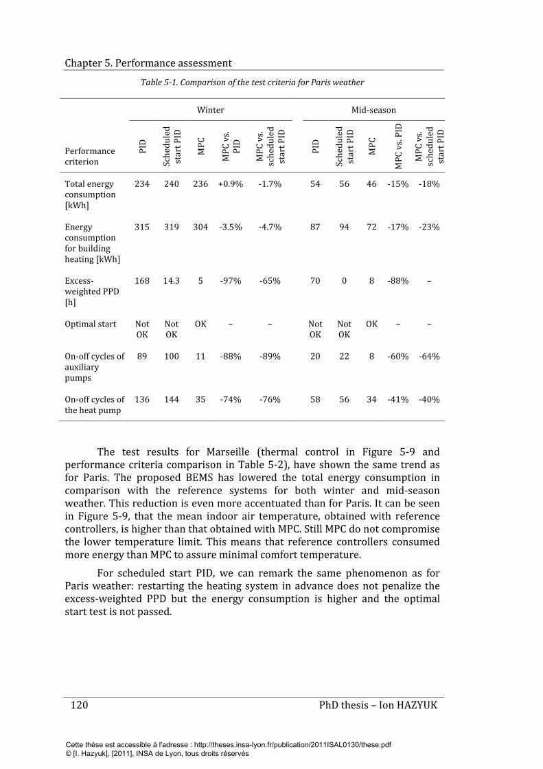
Chapter 5. Performance assessment
120 PhD thesis – Ion HAZYUK
Table 5-1. Comparison of the test criteria for Paris weather
Performance criterion
Winter Mid-season
PID
Sche
dule
d st
art P
ID
MPC
MPC
vs.
PID
MPC
vs.
sche
dule
d st
art P
ID
PI
D
Sche
dule
d st
art P
ID
MPC
MPC
vs.
PID
MPC
vs.
sche
dule
d st
art P
ID
Total energy consumption [kWh]
234 240 236 +0.9%
-1.7% 54 56 46 -15% -18%
Energy consumption for building heating [kWh]
315 319 304 -3.5% -4.7% 87 94 72 -17% -23%
Excess-weighted PPD [h]
168 14.3 5 -97% -65% 70 0 8 -88% –
Optimal start Not OK
Not OK
OK – – Not OK
Not OK
OK – –
On-off cycles of auxiliary pumps
89 100 11 -88% -89% 20 22 8 -60% -64%
On-off cycles of the heat pump
136 144 35 -74% -76% 58 56 34 -41% -40%
The test results for Marseille (thermal control in Figure 5-9 and performance criteria comparison in Table 5-2), have shown the same trend as for Paris. The proposed BEMS has lowered the total energy consumption in comparison with the reference systems for both winter and mid-season weather. This reduction is even more accentuated than for Paris. It can be seen in Figure 5-9, that the mean indoor air temperature, obtained with reference controllers, is higher than that obtained with MPC. Still MPC do not compromise the lower temperature limit. This means that reference controllers consumed more energy than MPC to assure minimal comfort temperature.
For scheduled start PID, we can remark the same phenomenon as for Paris weather: restarting the heating system in advance does not penalize the excess-weighted PPD but the energy consumption is higher and the optimal start test is not passed.
Cette thèse est accessible à l'adresse : http://theses.insa-lyon.fr/publication/2011ISAL0130/these.pdf © [I. Hazyuk], [2011], INSA de Lyon, tous droits réservés

Chapter 5. Performance assessment
PhD thesis – Ion HAZYUK 121
Figure 5-9. Comparisons of the indoor temperature evolution obtained with PID, scheduled start
PID and MPC controllers for (a) winter and (b) mid season Marseille weather
Table 5-2. Comparison of the test criteria for Marseille weather
Performance criterion
Winter Mid-season
PID
Sche
dule
d st
art P
ID
MPC
MPC
Vs
. PID
MPC
vs.
sche
dule
d st
art P
ID
PI
D
Sche
dule
d st
art P
ID
MPC
MPC
vs.
PID
MPC
vs.
sche
dule
d st
art P
ID
Total energy consumption [kWh]
138 142 116 -15.9%
-18.3% 22 22 18 -18.2% -18.2%
Energy consumption for building heating [kWh]
214 222 192 -10.3% -13.5% 36 36 30 -16.7% -16.7%
Excess-weighted PPD [h]
95 0 10 -89.5% – 15 0 13 -13.3% –
Optimal start Not OK
Not OK
OK – – OK Not OK
OK – –
On-off cycles of auxiliary pumps
90 96 10 -88.9% -89.6% 11 8 6 -45.5% -25%
On-off cycles of the heat pump
118 123 27 -77.1% -78% 45 42 36 -20% -14.3%
The conclusion that can be drawn after analysing the test results is that MPC always outperforms PID and scheduled start PID controllers regarding
Cette thèse est accessible à l'adresse : http://theses.insa-lyon.fr/publication/2011ISAL0130/these.pdf © [I. Hazyuk], [2011], INSA de Lyon, tous droits réservés
Chapter 5. Performance assessment
122 PhD thesis – Ion HAZYUK
comfort versus energy consumption. If the building model, occupation schedule and weather forecast are correct, MPC assures the comfort with minimal energy consumption, i.e. it is not possible to assure the same comfort consuming less energy. MPC is able to adapt the command to the whether, occupation type and current system state, with the condition that we have in advance information about future evolution of the weather and the occupation. Scheduled start PID restarts the heating before, but this is a fix time interval; it is calculated for a particular situation, which can be the worst or the most frequent case. Contrary to MPC, it cannot adapt to the exterior conditions (e.g. weather) to calculate the optimal command for the entire heating season. In other words, MPC guarantees optimal command that assures the comfort with minimal energy consumption for the entire heating season, and PID or scheduled start PID cannot guarantee this performance. Therefore, the BEMS based on MPC can achieve optimal comfort with minimal energy consumption.
5.7 Conclusions
The designed controller in Chapter 4 calculates the radiator inlet water temperature that satisfies the thermal comfort and minimizes the energy consumption. However, the hydraulic heating system that assures the availability of the hot water needs a BEMS. Therefore, in order to evaluate the real impact of the proposed MPC controller on the building, we needed to integrate it in a BEMS.
We proposed a BEMS and tested its performance for five day periods in winter and mid season weather for oceanic (Paris) and Mediterranean (Marseille) climates. The BEMS, including the proposed MPC, was implemented in a controller prototype and the tests were done in real time. The building and the hydraulic heating system were emulated and the communication with the controller was done via a data acquisition system. The performance assessment consisted in the comparison of the obtained performance with those of two classical solutions, against some standard performance criteria. The classical solutions were BEMS based on PID and scheduled start PID controllers and the regarded performance concerned the thermal comfort, the total energy consumption and the number of on-off cycles of the elements of the hydraulic heating system. The performance comparison has shown that MPC has drastically reduced the thermal discomfort, significantly reduced the number of on-off cycles of the hydraulic and heating pumps, and almost always reduced the energy consumption. For a period of five days, we managed to reduce the excess-weighted PPD up to 97 % compared to PID controller and up to 65 % compared to scheduled start PID controller while still reducing the energy consumption for building heating in this period by 3.5 % compared to PID controller and by 4.7 % compared to scheduled start PID controller. Also, by using the MPC, the number of on-off cycles of the heat pump was reduced from 144 (corresponding to scheduled start PID) to 35 cycles, for winter season in Paris while the number of on-off cycles of the auxiliary hydraulic pumps was reduced from 100 (corresponding to scheduled start PID) to 11 cycles, for the
Cette thèse est accessible à l'adresse : http://theses.insa-lyon.fr/publication/2011ISAL0130/these.pdf © [I. Hazyuk], [2011], INSA de Lyon, tous droits réservés

Chapter 5. Performance assessment
PhD thesis – Ion HAZYUK 123
same period. The number of on-off cycles of heat pump and auxiliary hydraulic pumps was reduced for all the performed tests in comparison with both classical solutions. The optimal start test was passed for all the test periods only by the MPC controller, which means that MPC is able to adapt to the actual meteorological conditions, while the other two tested controllers cannot do this.
Cette thèse est accessible à l'adresse : http://theses.insa-lyon.fr/publication/2011ISAL0130/these.pdf © [I. Hazyuk], [2011], INSA de Lyon, tous droits réservés
Chapter 5. Performance assessment
124 PhD thesis – Ion HAZYUK
References
CEN (2001). EN 12098-2:2001: Controls for heating systems - Part 2: Optimum start-stop control equipment for hot water heating systems. Brussels, Belgium: European Committee for Standardization.
CEN (2005). EN ISO 7730:2005: Ergonomics of the thermal environment - Analytical determination and interpretation of thermal comfort using calculation of the PMV and PPD indices and local thermal comfort criteria. Brussels, Belgium: European Committee for Standardization.
CEN (2007). EN 15251:2007: Indoor environmental input parameters for design and assessment of energy performance of buildings addressing indoor air quality, thermal environment, lighting and acoustics. Brussels, Belgium: European Committee for Standardization.
CSTB (2005). RT-2005: Réglementation Thermique 2005. Paris, France: Centre Scientifique et Technique du Bâtiment.
David, R. & Alla, H. (1992). Petri Nets and Grafcet: Tools for Modeling Discrete Event Systems. New York, NY: Prentice Hall.
Dounis, A. I. & Caraiscos, C. (2009). Advanced control systems engineering for energy and comfort management in a building environment--A review. Renewable and Sustainable Energy Reviews, 13(6-7), 1246-1261.
Fanger, P. O. (1972). Thermal Comfort Analysis and Application in Environmental Design. New York, NY: McGraw-Hill.
Ghoul, E. (1999). Retrofit in hydraulic matching: Behaviour of water flowrate of decoupling bottles in a distribution meshed network. Chauffage, Ventilation, Conditionnement d'Air, 7(8), 36-41.
Husaunndee, A., Lahrech, R., Vaezi-Nejad, H. & Visier, J. C. (1997). SIMBAD: A simulation toolbox for the design and test of HVAC control systems. In: 5th international IBPSA conference, September 8-10, 1997, Prague, Czech Republic.
Liao, Z., Swainson, M. & Dexter, A. L. (2005). On the control of heating systems in the UK. Building and Environment, 40(3), 343-351.
Peeters, L., Van der Veken, J., Hens, H., Helsen, L. & D'Haeseleer, W. (2008). Control of heating systems in residential buildings: Current practice. Energy and Buildings, 40(8), 1446-1455.
Ziegler, J. G. & Nichols, N. B. (1942). Optimum settings for automatic controllers. Tsaction of the ASME, 64, 759-768.
Cette thèse est accessible à l'adresse : http://theses.insa-lyon.fr/publication/2011ISAL0130/these.pdf © [I. Hazyuk], [2011], INSA de Lyon, tous droits réservés
125
Conclusions and outlooks
An effective integration of renewable energies in buildings passes through three essential stages. These are the system design, its sizing and control. Today, the design of building energetic systems is based exclusively on expert’s experience. The expert proposes several system configurations, which in his opinion fit better for the given building, and then evaluates the proposed alternatives through dynamic simulations. Thought dynamic simulation gives the most realistic results for system evaluation, the current practices of using this tool do not guarantee the optimal choice of the system.
The first problem occurs in the case of intermittently occupied buildings, where there are at least two set-point temperatures. In order to assess the heating load of the building, to use it for system sizing, today it is considered that the indoor temperature follows exactly its set-point. This hypothesis makes the peak load depend on the simulation sampling time. This is not desirable because it may lead to ill-sized equipment.
Another problem arises when there is a comparison of two different system configurations. In order to be able to say that a system performs better that the other one, both systems must be optimized (optimally sized and optimally controlled). Unfortunately, today during the simulation process, the controllers are not optimized; this may be the main cause of the poor performance of the system. When speaking of the control system, there can be distinguished two such systems. The first controller handles the multi-source system and the second one regulates the indoor temperature. Both control systems have an important impact on the multisource system performance. Concerning the control system that regulates the indoor temperature, today the most promising solution is Model Predictive Control. Nevertheless, the use of the classical cost function, actually used in temperature control, does not minimize the energy consumption.
To avoid the drawbacks resulting from the assumption that the indoor temperature follows exactly its set-point, we proposed to transform the heating load assessment problem into a control problem. The building is considered as a thermal system disturbed by the weather, where the regulator calculates the necessary heat to control the indoor temperature. The heat flux, calculated by
Cette thèse est accessible à l'adresse : http://theses.insa-lyon.fr/publication/2011ISAL0130/these.pdf © [I. Hazyuk], [2011], INSA de Lyon, tous droits réservés
Conclusions and outlooks
126 PhD thesis – Ion HAZYUK
the regulator, actually represents the heating load of the building. Its calculation is based on the real evolution of the indoor temperature and not on its set-point. Therefore, the simulation sampling time will not influence the resulted heating load, even if the set-point temperature changes in step-like waveform.
In intermittently occupied buildings, usually there are at least two set-point temperatures within 24 hours. In this case, the ability of the heating system to recover the building from setback is very important. Therefore, for heating load calculation, we proposed a Model Predictive Programming (MPP) strategy, which is a modification of Model Predictive Control (MPC). The main differences between MPP and MPC is that MPP is an optimization without constraints (except the one of positive command) and the command is calculated only once, without state feedback. The proposed MPP is able to restart the heating system in advance in order to assure the thermal comfort at the very beginning of the occupation period. Used together with the feed-forward control technique, it is able to use weather forecast for the optimization of the energy consumption. We also have found, through MPP, that there is a trade-off between the peak load and the consumed energy for heating; the larger the peak load the smaller the energy consumption. The optimization must be done for a time horizon (ex. 10 years) for which is minimized the investment and the operating costs. Thus, MPP gives a framework for this optimization, where the user must tune a parameter, called “relaxation time”.
The information required by MPP is the building model, the free gains, variation of ventilation rate and data records of the local weather. As this tool is intended to be used mainly in the design stage of the building, the building model can be identified using input/output data records obtained by simulation. Records of local weather are also available in dedicated simulation tools as Trnsys, Simbad, etc.
The limits of our contribution consists in the choice of the optimal relaxation time, which would optimize the total cost of the system for a given time period. Thus, future developments in this direction present potential interest. Also, in the optimized cost function, it is minimized the square of the command increment (i.e. heat flux). This criterion does not represent thermal energy and therefore MPP does not assure minimal energy consumption.
Concerning the control system, we proposed a thermal controller which assures thermal comfort with minimal energy consumption. The proposed controller is a MPC which uses weather forecast for optimal temperature control. Here, our contribution is the new proposed cost function for MPC, along with the suggested solving algorithm for the optimization problem.
Unlike the classical cost function, the proposed one minimizes the future command subject to constraints on the heat flux and indoor temperature. The minimization of the command, instead of its squared increment, assures minimal energy consumption. The constraints on the heat flux (or equivalently on the radiator inlet water temperature) take into consideration the maximal potential of the heating system in order to assure the required performance.
Cette thèse est accessible à l'adresse : http://theses.insa-lyon.fr/publication/2011ISAL0130/these.pdf © [I. Hazyuk], [2011], INSA de Lyon, tous droits réservés
Conclusions and outlooks
PhD thesis – Ion HAZYUK 127
The constraints on the indoor temperature assure the thermal comfort in the building.
The proposed cost function also eliminates the drawbacks of the trade-off principle and of the use of the set-point temperature instead of temperature range, which are present when using the classical cost function. When trade-off principle is used, we may obtain different results, depending on what was preferred (comfort or energy savings). Also, there is an additional tuning parameter, which must be chosen. By forcing the indoor temperature to follow a set-point instead of letting it float in an accepted temperature range results in consuming more energy than it is necessary. The proposed cost function lets the temperature float in a predefined temperature range and does not sacrifice the comfort in the detriment of energy savings. By using the proposed cost function, the heating system will take into account the building inertia and weather forecast to maintain the minimal comfort with minimal energy consumption.
Another contribution is the idea to use physical knowledge in order to improve the control performance. The first place where this technique is used is the parameter identification of the building model. Optimal control is a model-based technique and therefore a system model is required. In this thesis, the building model is obtained in two steps. Firstly, a low order model structure is obtained from physical considerations, and then, its parameters are obtained by least squares identification. This combination gives actually a projection of the complex and high-order building model on a low order structure gathered from physical representation of the building thermal behavior. By doing so, we obtain a robust model. The second place where physical knowledge is used is to overcome the nonlinearity in the building model. We firstly identified the nonlinear characteristic and then we proposed a method to use this characteristic for model linearization. The proposed linearization made the system model valid on the entire operating range, not just around some operating point, as in classical local linearization.
For the multisource system, we proposed a Building Energy Management System (BEMS), which considers information from the MPC command. This permits the BEMS to use the energy resources more effectively. Yet, the proposed BEMS is not an optimal controller, so additional improvements are achievable.
We tested the proposed MPC and compared the obtained results with those of well tuned PID controllers, which today are state of the art on the market. The comparison was done against criteria suggested by European regulation. In all the tests, MPC performed the best, assuring the thermal comfort and consuming less energy. Moreover, the command calculated by MPC was less aggressive, which extends the life span of expensive equipments such as hydraulic pumps and heat pumps.
Nevertheless, these good results were obtained mostly because we owned an accurate model of the building. In real life, the building model identification is not as simple as for other systems. Many constraints do not
Cette thèse est accessible à l'adresse : http://theses.insa-lyon.fr/publication/2011ISAL0130/these.pdf © [I. Hazyuk], [2011], INSA de Lyon, tous droits réservés

Conclusions and outlooks
128 PhD thesis – Ion HAZYUK
permit to excite the building modes as it would be necessary, so the accuracy of the identified model can diminish. This can degrade the obtained results of the control performances. Therefore, this is a direction for further researches, and the present thesis provides evidences for its benefits.
Thus, the theses of this manuscript are the following:
I) In order to control a system, we need to comprehend that system (have a model adapted for control). It is desirable to have a physical model (based on the physics of the phenomenon – white-box or grey-box models)
II) The control is an inverse problem, which also can be used for system sizing.
III) In the case of thermal systems, the quadratic criterion is incorrect when the command signal is the heat flux. A linear criterion minimizes the energy.
IV) A robust model is obtained when the identification is a projection on a structure based on physical knowledge.
V) Using physical knowledge for model linearization, we can obtain a linearized model which is valid on the entire operating range
Cette thèse est accessible à l'adresse : http://theses.insa-lyon.fr/publication/2011ISAL0130/these.pdf © [I. Hazyuk], [2011], INSA de Lyon, tous droits réservés

Cette thèse est accessible à l'adresse : http://theses.insa-lyon.fr/publication/2011ISAL0130/these.pdf © [I. Hazyuk], [2011], INSA de Lyon, tous droits réservés
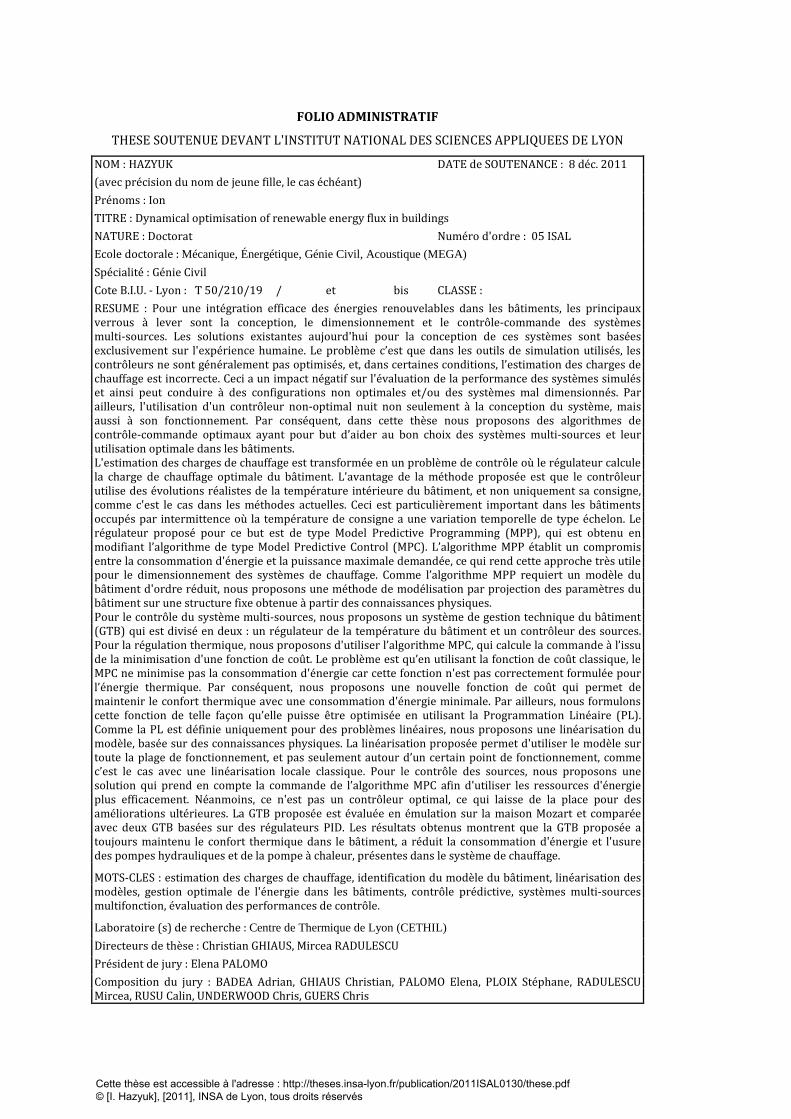
FOLIO ADMINISTRATIF
THESE SOUTENUE DEVANT L'INSTITUT NATIONAL DES SCIENCES APPLIQUEES DE LYON
NOM : HAZYUK DATE de SOUTENANCE : 8 déc. 2011 (avec précision du nom de jeune fille, le cas échéant) Prénoms : Ion TITRE : Dynamical optimisation of renewable energy flux in buildings NATURE : Doctorat Numéro d'ordre : 05 ISAL Ecole doctorale : Mécanique, Énergétique, Génie Civil, Acoustique (MEGA) Spécialité : Génie Civil Cote B.I.U. - Lyon : T 50/210/19 / et bis CLASSE : RESUME : Pour une intégration efficace des énergies renouvelables dans les bâtiments, les principaux verrous à lever sont la conception, le dimensionnement et le contrôle-commande des systèmes multi-sources. Les solutions existantes aujourd'hui pour la conception de ces systèmes sont basées exclusivement sur l'expérience humaine. Le problème c’est que dans les outils de simulation utilisés, les contrôleurs ne sont généralement pas optimisés, et, dans certaines conditions, l’estimation des charges de chauffage est incorrecte. Ceci a un impact négatif sur l'évaluation de la performance des systèmes simulés et ainsi peut conduire à des configurations non optimales et/ou des systèmes mal dimensionnés. Par ailleurs, l'utilisation d'un contrôleur non-optimal nuit non seulement à la conception du système, mais aussi à son fonctionnement. Par conséquent, dans cette thèse nous proposons des algorithmes de contrôle-commande optimaux ayant pour but d’aider au bon choix des systèmes multi-sources et leur utilisation optimale dans les bâtiments. L'estimation des charges de chauffage est transformée en un problème de contrôle où le régulateur calcule la charge de chauffage optimale du bâtiment. L'avantage de la méthode proposée est que le contrôleur utilise des évolutions réalistes de la température intérieure du bâtiment, et non uniquement sa consigne, comme c'est le cas dans les méthodes actuelles. Ceci est particulièrement important dans les bâtiments occupés par intermittence où la température de consigne a une variation temporelle de type échelon. Le régulateur proposé pour ce but est de type Model Predictive Programming (MPP), qui est obtenu en modifiant l’algorithme de type Model Predictive Control (MPC). L’algorithme MPP établit un compromis entre la consommation d'énergie et la puissance maximale demandée, ce qui rend cette approche très utile pour le dimensionnement des systèmes de chauffage. Comme l’algorithme MPP requiert un modèle du bâtiment d'ordre réduit, nous proposons une méthode de modélisation par projection des paramètres du bâtiment sur une structure fixe obtenue à partir des connaissances physiques. Pour le contrôle du système multi-sources, nous proposons un système de gestion technique du bâtiment (GTB) qui est divisé en deux : un régulateur de la température du bâtiment et un contrôleur des sources. Pour la régulation thermique, nous proposons d'utiliser l’algorithme MPC, qui calcule la commande à l’issu de la minimisation d'une fonction de coût. Le problème est qu’en utilisant la fonction de coût classique, le MPC ne minimise pas la consommation d'énergie car cette fonction n'est pas correctement formulée pour l’énergie thermique. Par conséquent, nous proposons une nouvelle fonction de coût qui permet de maintenir le confort thermique avec une consommation d'énergie minimale. Par ailleurs, nous formulons cette fonction de telle façon qu’elle puisse être optimisée en utilisant la Programmation Linéaire (PL). Comme la PL est définie uniquement pour des problèmes linéaires, nous proposons une linéarisation du modèle, basée sur des connaissances physiques. La linéarisation proposée permet d'utiliser le modèle sur toute la plage de fonctionnement, et pas seulement autour d’un certain point de fonctionnement, comme c’est le cas avec une linéarisation locale classique. Pour le contrôle des sources, nous proposons une solution qui prend en compte la commande de l’algorithme MPC afin d'utiliser les ressources d'énergie plus efficacement. Néanmoins, ce n'est pas un contrôleur optimal, ce qui laisse de la place pour des améliorations ultérieures. La GTB proposée est évaluée en émulation sur la maison Mozart et comparée avec deux GTB basées sur des régulateurs PID. Les résultats obtenus montrent que la GTB proposée a toujours maintenu le confort thermique dans le bâtiment, a réduit la consommation d'énergie et l'usure des pompes hydrauliques et de la pompe à chaleur, présentes dans le système de chauffage.
MOTS-CLES : estimation des charges de chauffage, identification du modèle du bâtiment, linéarisation des modèles, gestion optimale de l'énergie dans les bâtiments, contrôle prédictive, systèmes multi-sources multifonction, évaluation des performances de contrôle.
Laboratoire (s) de recherche : Centre de Thermique de Lyon (CETHIL) Directeurs de thèse : Christian GHIAUS, Mircea RADULESCU Président de jury : Elena PALOMO Composition du jury : BADEA Adrian, GHIAUS Christian, PALOMO Elena, PLOIX Stéphane, RADULESCU Mircea, RUSU Calin, UNDERWOOD Chris, GUERS Chris
Cette thèse est accessible à l'adresse : http://theses.insa-lyon.fr/publication/2011ISAL0130/these.pdf © [I. Hazyuk], [2011], INSA de Lyon, tous droits réservés