dynamical systems associated to separated graphs, graph algebras, and paradoxical decompositions
TRANSCRIPT

Available online at www.sciencedirect.com
ScienceDirect
Advances in Mathematics 252 (2014) 748–804www.elsevier.com/locate/aim
Dynamical systems associated to separated graphs,graph algebras, and paradoxical decompositions ✩
Pere Ara a,∗, Ruy Exel b
a Departament de Matemàtiques, Universitat Autònoma de Barcelona, 08193 Bellaterra (Barcelona), Spainb Departamento de Matemática, Universidade Federal de Santa Catarina, 88010-970 Florianópolis, SC, Brazil
Received 29 October 2012; accepted 3 November 2013
Communicated by Dan Voiculescu
Abstract
We attach to each finite bipartite separated graph (E,C) a partial dynamical system (Ω(E,C),F, θ),where Ω(E,C) is a zero-dimensional metrizable compact space, F is a finitely generated free group,and θ is a continuous partial action of F on Ω(E,C). The full crossed product C∗-algebra O(E,C) =C(Ω(E,C)) �θ∗ F is shown to be a canonical quotient of the graph C∗-algebra C∗(E,C) of the sepa-rated graph (E,C). Similarly, we prove that, for any ∗-field K , the algebraic crossed product Lab
K(E,C) =
CK(Ω(E,C))�algθ∗ F is a canonical quotient of the Leavitt path algebra LK(E,C) of (E,C). The monoid
V(LabK
(E,C)) of isomorphism classes of finitely generated projective modules over LabK
(E,C) is explicitlycomputed in terms of monoids associated to a canonical sequence of separated graphs. Using this, we areable to construct an action of a finitely generated free group F on a zero-dimensional metrizable compactspace Z such that the type semigroup S(Z,F,K) is not almost unperforated, where K denotes the algebraof clopen subsets of Z. Finally we obtain a characterization of the separated graphs (E,C) such that thecanonical partial action of F on Ω(E,C) is topologically free.© 2013 Elsevier Inc. All rights reserved.
MSC: primary 16D70, 46L35; secondary 06A12, 06F05, 46L80
✩ The first named author was partially supported by DGI MICIIN–FEDER MTM2011-28992-C02-01, and by theComissionat per Universitats i Recerca de la Generalitat de Catalunya. The second named author was partially supportedby CNPq.
* Corresponding author.E-mail addresses: [email protected] (P. Ara), [email protected] (R. Exel).
0001-8708/$ – see front matter © 2013 Elsevier Inc. All rights reserved.http://dx.doi.org/10.1016/j.aim.2013.11.009

P. Ara, R. Exel / Advances in Mathematics 252 (2014) 748–804 749
Keywords: Graph algebra; Dynamical system; Refinement monoid; Nonstable K-theory; Partial representation; Partialaction; Crossed product; Condition (L)
Contents
1. Introduction . . . . . . . . . . . . . . . . . . . . . . . . . . . . . . . . . . . . . . . . . . . . . . . . . . . . . . . . 7492. Preliminary definitions . . . . . . . . . . . . . . . . . . . . . . . . . . . . . . . . . . . . . . . . . . . . . . . . . 7533. Multiresolutions . . . . . . . . . . . . . . . . . . . . . . . . . . . . . . . . . . . . . . . . . . . . . . . . . . . . . . 7544. Bipartite separated graphs . . . . . . . . . . . . . . . . . . . . . . . . . . . . . . . . . . . . . . . . . . . . . . . 7575. The main construction . . . . . . . . . . . . . . . . . . . . . . . . . . . . . . . . . . . . . . . . . . . . . . . . . . 7616. Dynamical systems . . . . . . . . . . . . . . . . . . . . . . . . . . . . . . . . . . . . . . . . . . . . . . . . . . . . 7697. The type semigroup . . . . . . . . . . . . . . . . . . . . . . . . . . . . . . . . . . . . . . . . . . . . . . . . . . . 7748. Descriptions of the space Ω(E,C) . . . . . . . . . . . . . . . . . . . . . . . . . . . . . . . . . . . . . . . . . 7829. Examples . . . . . . . . . . . . . . . . . . . . . . . . . . . . . . . . . . . . . . . . . . . . . . . . . . . . . . . . . . 790
10. Topologically free actions . . . . . . . . . . . . . . . . . . . . . . . . . . . . . . . . . . . . . . . . . . . . . . . 796Acknowledgments . . . . . . . . . . . . . . . . . . . . . . . . . . . . . . . . . . . . . . . . . . . . . . . . . . . . . . . . . 802References . . . . . . . . . . . . . . . . . . . . . . . . . . . . . . . . . . . . . . . . . . . . . . . . . . . . . . . . . . . . . . 802
1. Introduction
In their seminal paper [18], J. Cuntz and W. Krieger gave a dynamical interpretation of theCuntz–Krieger algebras associated to square {0,1}-matrices in terms of the corresponding sub-shifts of finite type. Since then, there has been a long and fruitful interaction between the theoryof combinatorially defined C∗-algebras and dynamics, see [21,40,39,26,38,12,29,11,46,55,49,50,48,28,25].
In [22, Section 5], the second named author describes any Cuntz–Krieger C∗-algebra as acrossed product of a commutative C∗-algebra by a partial action of a non-abelian free group.The same applies to graph C∗-algebras, which are generalizations of Cuntz–Krieger algebras.
A wider class of graph algebras has been introduced in [8] and [7]. These algebras are attachedto separated graphs, where a separated graph is a pair (E,C) consisting of a directed graph E
and a set C =⊔v∈E0 Cv , where each Cv is a partition of the set of edges whose terminal ver-tex is v. Their associated graph C∗-algebras C∗(E,C) and Leavitt path algebras LK(E,C) (foran arbitrary field K) provide generalizations of the usual graph C∗-algebras [47] and Leavittpath algebras [2,10] associated to directed graphs, although these algebras behave quite differ-ently from the usual graph algebras because the range projections associated to different edgesneed not commute. One motivation for their introduction was to provide graph-algebraic modelsfor the Leavitt algebras LK(m,n) of [41], and the C∗-algebras Unc
m,n studied by L. Brown [17]and McClanahan [42–44]. Another motivation was to obtain graph algebras whose structure ofprojections is as general as possible. Thanks to deep results due to G.M. Bergman [13,14], itis possible to show that the natural map M(E,C) → V(LK(E,C)) from a monoid M(E,C)
naturally associated to (E,C) to the monoid V(LK(E,C)) of isomorphism classes of finitelygenerated projective right modules over LK(E,C) is an isomorphism, see [8, Theorem 4.3].Since each conical abelian monoid M is isomorphic to a monoid of the form M(E,C) for asuitable separated graph (E,C) [8, Proposition 4.4], we conclude that Leavitt path algebras ofseparated graphs realize all the conical abelian monoids. (By the results of [10], this is not true forthe class of Leavitt path algebras of non-separated graphs.) The first author and Ken Goodearl

750 P. Ara, R. Exel / Advances in Mathematics 252 (2014) 748–804
raised in [7] the problem of whether the natural map M(E,C) → V(C∗(E,C)) is an isomor-phism (see also [4, Section 6] for a brief discussion on this problem).
Recall that a set S of partial isometries in a ∗-algebra A is said to be tame [24, Proposition 5.4]if every element of U = 〈S ∪ S∗〉, the multiplicative semigroup generated by S ∪ S∗, is a partialisometry, and the set {e(u) | u ∈ U} of final projections of the elements of U is a commutingset of projections of A. A main difficulty in working with C∗(E,C) and LK(E,C) is that, ingeneral, the generating set of partial isometries of these algebras is not tame. This is not thecase for the usual graph algebras, where it can be easily shown that the generating set of partialisometries is tame.
The main objective of the present paper is to associate a partial dynamical system to any fi-nite bipartite separated graph (E,C), and to uncover some of the fundamental properties of thecrossed products corresponding to it. To a large extent, this task can be made simultaneouslyin the purely algebraic category and in the C∗-algebraic category. However, several analyticaspects, such as the study of exactness, nuclearity and reduced crossed products will needmore specific tools. This dynamical system is described by the action θ of a finitely generatedfree non-abelian group F, whose rank coincides with the number of edges of E, on a zero-dimensional metrizable compact space Ω(E,C). The corresponding C∗-algebra full crossedproduct O(E,C) := C(Ω(E,C)) �θ∗ F is shown to coincide with a canonical quotient of thegraph C∗-algebra C∗(E,C) of the separated graph (E,C) (Corollary 6.12). Namely we obtainan isomorphism
C(Ω(E,C)
)�θ∗ F ∼= C∗(E,C)/J
where J is the closed ideal of C∗(E,C) generated by all the commutators [e(γ ), e(μ)], whereγ,μ belong to the multiplicative semigroup U of C∗(E,C) generated by the canonical par-tial isometries, corresponding to E1 ∪ (E1)∗. Note that E1 ∪ (E1)∗ becomes a tame set ofpartial isometries in O(E,C). The ideal J is the closure of an increasing union of ideals Jn,with Jn the ideal generated by all the commutators [e(γ ), e(μ)], where γ,μ can be expressedas products of � n canonical generators. We show in Section 5 that there is a canonical se-quence {(En,C
n)} of finite bipartite separated graphs such that C∗(E,C)/Jn∼= C∗(En,C
n)
for all n. Consequently the C∗-algebra O(E;C) = C∗(E,C)/J is isomorphic to an inductivelimit lim−→n
C∗(En,Cn) with surjective transition maps. This gives an approximation result of
the dynamical C∗-algebra O(E,C) by graph C∗-algebras of separated graphs. We also con-sider in Section 10 a reduced C∗-algebra Or (E,C), which is defined in terms of the reducedcrossed product of C(Ω(E,C)) by F. These C∗-algebras have been studied in detail in [5] inthe case where (E,C) = (E(m,n),C(m,n)) is the separated graph whose graph C∗-algebra isMorita-equivalent to MacClanahan’s algebras Unc
m,n (see Example 9.3 for the definition), underthe notations Om,n and Or
m,n. They are attached to the so-called universal (m,n)-dynamical sys-tem, see [5, Theorem 3.8]. It is shown in [5] that the natural map Om,n → Or
m,n is not injective.A similar result holds when we work in the category of ∗-algebras, obtaining a corresponding
isomorphism
CK
(Ω(E,C)
)�alg
θ∗ F∼= LK(E,C)/J ∼= lim−→LK
(En,C
n),
where CK(Ω(E,C)) is the ∗-algebra of continuous functions from Ω(E,C) to the ∗-field K
endowed with the discrete topology, and the crossed product is taken in the algebraic cate-gory. We denote this quotient ∗-algebra LK(E,C)/J by Lab
K (E,C). (Here, of course, J meansthe algebraic ideal generated by the commutators [e(γ ), e(μ)], for γ,μ ∈ U .) This leads to amonoid isomorphism V(Lab(E,C)) ∼= lim V(LK(En,C
n)) ∼= lim M(En,Cn). Conjecturally,
K −→n −→n
P. Ara, R. Exel / Advances in Mathematics 252 (2014) 748–804 751
the same monoid lim−→nM(En,C
n) would compute the nonstable K-theory of O(E,C). The
monoid R(E,C) := lim−→M(En,Cn) is a refinement monoid (see Section 2 for the definition) and
the natural map M(E,C) → R(E,C) gives a canonical refinement of M(E,C) (Lemma 4.5).This condition implies in particular that the map M(E,C) →R(E,C) is an order-embedding.
We remark that there is no loss of generality in assuming that our separated graphs arebipartite, as we show in Proposition 9.1 that every graph algebra of a separated graph is Morita-equivalent to a graph algebra of a bipartite separated graph.
As a biproduct of our results, we are able to answer a question raised in recent papers byKerr [36], Kerr and Nowak [37], and Rørdam and Sierakowski [52]. The statement of this ques-tion is unrelated to graph algebras but, using our new theory, we can give a complete answer toit. The classical Tarski’s Theorem [57, Corollary 9.2] asserts that, for an action of a group G on aset X, a subset E of X is not G-paradoxical if and only if there is a finitely additive G-invariantmeasure μ :P(X) → [0,∞] such that μ(E) = 1. This result follows from special properties ofthe type semigroup S(X,G) of the action. Observe that the set of finitely additive G-invariantmeasures μ as above is precisely the state space of (S(X,G), [E]).
If G is a discrete group acting by continuous transformations on a topological space X andD is a G-invariant subalgebra of subsets of X, one may restrict the equidecomposability relationto subsets in D, obtaining a “relative” type semigroup S(X,G,D), as in [36,37,52]. Of partic-ular interest is the case where X is a zero-dimensional metrizable compact space and D is thesubalgebra K of clopen subsets of X. It has been asked in the above-mentioned papers (cf. [52,page 285], [36, Question 3.10]) whether the analogue of Tarski’s Theorem holds in this moregeneral context, that is, whether for E ∈ K we have that 2[E] � [E] in S(X,G,K) if and onlyif the state space of (S(X,G,K), [E]) is non-empty. We show in Corollary 7.12 that the answerto this question is negative. Indeed, our Theorem 7.11 implies that S(X,G,K) does not satisfyin general any cancellation or order-cancellation law, since, given any finitely generated conicalabelian monoid M we can find a triple (X,G,K), with X a 0-dimensional metrizable compactspace, such that there is an order-embedding of M into S(X,G,K). Our methods give in a nat-ural way partial actions of discrete groups on totally disconnected spaces. We use globalizationresults from [1] to reach the desired goal with global actions.
We also obtain a characterization of the finite bipartite separated graphs (E,C) such that thecanonical action of the free group F on the space Ω(E,C) is topologically free. It turns out thatthis is equivalent to a version, adapted to separated graphs, of the well-known condition (L) forgraphs, which is the condition that every cycle has an entry ([39], [26, Definition 12.1]), see The-orem 10.5. Using this result and known facts on crossed products by partial actions from [27]we show that, if (E,C) satisfies condition (L), then the reduced crossed product C∗-algebraOr (E,C) = C(Ω(E,C)) �r F satisfies condition (SP), that is, every nonzero hereditary subal-gebra contains a nonzero projection, see Theorem 10.9. A corresponding result is also shown forthe algebra Lab
K (E,C) (Theorem 10.10 and Remark 10.11).Many properties of these new classes of algebras remain to be investigated. We mention the
computation of K-theoretic invariants in terms of the separated graph (E,C), the study of thestructure of ideals, and the study of exactness and nuclearity. Topologically free minimal orbits ofthe topological space Ω(E,C) with respect to the canonical action of the free group will surelyprovide examples of simple C∗-algebras with exotic properties. In a different direction, the al-gebras constructed in the present paper represent a further step in the strategy initiated in [8] toconstruct von Neumann regular rings and exchange rings with prescribed V-monoids (see [3]for a survey on this problem). This will be discussed in more detail in [9], where the refine-ment monoid R(E,C) = limM(En,C
n) associated to the separated graph (E,C) described in
−→
752 P. Ara, R. Exel / Advances in Mathematics 252 (2014) 748–804
Example 9.6 will be realized as the V-monoid of an exchange K-algebra obtained as a universallocalization of the corresponding algebra Lab
K (E,C). The latter algebra is Morita equivalent tothe algebra of the free monogenic inverse semigroup (see Example 9.6).
1.1. Contents
We now explain in more detail the contents of this paper. In Section 2 we recall the basicdefinitions needed for our work, coming from the papers [7] and [8]. Section 3 contains somepreparatory material concerning graph theory and semigroup theory. In particular we introducethe crucial concept of a multiresolution of a separated graph (E,C) at a set of vertices V of E.This is a modification of the concept of resolution of a separated graph at a set of vertices, whichhas been introduced in [8, Section 8]. As in [8], the aim to introduce this concept is to giveembeddings of the monoid M(E,C) associated to a separated graph (E,C) into a refinementmonoid corresponding to another separated graph (F,D), given in general as the limit of an infi-nite sequence of separated graphs obtained by successive applications of the resolution process.The multiresolution process differs from the resolution process in that it involves at once all thesets in the corresponding partitions Cv , v ∈ V , and so it does not depend on the particular choiceof pairs X,Y ∈ Cv , for v ∈ V . In Section 4, we define, for a given finite bipartite separated graph(E,C), a canonical sequence of finite separated graphs (Fn,D
n), obtained by successive appli-cations of the multiresolution process, in such a way that the union (F∞,D∞) =⋃∞
n=0(Fn,Dn)
satisfies that M(F∞,D∞) is a refinement of M(E,C). The canonical sequence {(En,Cn)} of
finite bipartite separated graphs obtained as the sections of (F∞,D∞) is of special importance.On one hand, it is shown in Lemma 4.5 that there are natural connecting homomorphismsιn :M(En,C
n) → M(En+1,Cn+1) such that M(F∞,D∞) ∼= lim−→n
(M(En,Cn), ιn), so that the
map M(E,C) → lim−→n(M(En,C
n), ιn) is a refinement of M(E,C). On the other hand, it is
shown in Theorem 5.7 that there is a natural isomorphism LK(E,C)/Jn∼= LK(En,C
n), whereJn is the ideal of LK(E,C) generated by all the commutators [e(γ ), e(μ)], where γ,μ are prod-ucts of � n canonical generators from E1 ∪ (E1)∗. A similar result holds for the correspondinggraph C∗-algebras. The notations Lab(E,C) and O(E,C) are introduced in Notation 5.8. Thetopological space Ω(E,C) is also introduced in Section 5 as the spectrum of the canonical com-mutative AF-subalgebra B0 of O(E,C).
We develop in Section 6 the crossed product structure of the algebras LabK (E,C) and O(E,C).
This is done in a soft way, using the universal properties of the involved objects. The topologicalspace Ω(E,C) is shown in Corollary 6.11 to be the universal (E,C)-dynamical system. Thisgives a different proof of [5, Theorem 3.8], where the particular case of (m,n)-dynamical sys-tems is considered. Moreover the natural partial action of the free group F = F〈E1〉 on Ω(E,C)
induces ∗-isomorphisms LabK (E,C) ∼= CK(Ω(E,C)) �α F and O(E,C) ∼= C(Ω(E,C)) �α F
(Corollary 6.12). Section 7 is devoted to the study of the type semigroups. Our main resultis Theorem 7.11, where it is shown that, given any finitely generated abelian conical monoidM there exists a 0-dimensional metrizable compact space Z and an action of a finitely gener-ated free group F on it so that M order-embeds in the type semigroup S(Z,F,K). This uses themachinery from Sections 3–6 plus Abadie’s globalization results [1]. In Section 8 we develop de-scriptions of the space Ω(E,C) and the canonical partial action of the free group F on it. Thereare two different descriptions, one in terms of configurations and another in terms of certain“choice functions”, called here E-functions. We show in Theorem 8.3 that the basic clopen setscorresponding to the vertices in the odd layers of the graph F∞ (introduced in Construction 4.4)correspond precisely to the partial E-functions. Several examples are presented in Section 9.

P. Ara, R. Exel / Advances in Mathematics 252 (2014) 748–804 753
Apart from the motivational example leading to the (m,n)-dynamical system (Example 9.3), weconsider various interesting examples which are connected with constructions already investi-gated in disparate contexts. So for example we recover Truss example from [56] of a G-spaceX with failure of the 2-cancellation law 2x = 2y ⇒ x = y in the type semigroup (Example 9.5),a separated graph (E,C) such that the algebra O(E,C) is Morita-equivalent to the C∗-algebra ofthe free monogenic inverse semigroup [34] (Example 9.6), and another separated graph (F,D)
such that O(F,D) (respectively LabK (F,D)) is Morita-equivalent to the group C∗-algebra of the
lamplighter group C∗(Z2 �Z) (respectively the group algebra K[Z2 �Z]). Finally, Section 10 con-tains our characterization of the finite bipartite separated graphs (E,C) such that the canonicalaction of the free group F on the space Ω(E,C) is topologically free and the consequences forthe algebraic structure of O(E,C) and Lab
K (E,C).After the first version of this paper was posted at arXiv, we have been informed by Fred
Wehrung that, by using results of H. Dobbertin, he has obtained a proof of the fact that anycountable conical refinement monoid with order-unit is isomorphic to a type semigroup of theform S(Z,F,K), where F is a countably generated free group.
2. Preliminary definitions
The concept of separated graph, introduced in [8], plays a vital role in our construction. In thissection, we will recall this concept and we will also recall the definitions of the monoid associatedto a separated graph, the Leavitt path algebra and the graph C∗-algebra of a separated graph.
We will use the reverse notation as in [8] and [7], but in agreement with the one used in [5],and in the book [47].
Definition 2.1. (See [8].) A separated graph is a pair (E,C) where E is a graph, C =⊔v∈E0 Cv ,and Cv is a partition of r−1(v) (into pairwise disjoint non-empty subsets) for every vertex v. (Incase v is a source, we take Cv to be the empty family of subsets of r−1(v).)
If all the sets in C are finite, we say that (E,C) is a finitely separated graph. This necessarilyholds if E is column-finite (that is, if r−1(v) is a finite set for every v ∈ E0).
The set C is a trivial separation of E in case Cv = {r−1(v)} for each v ∈ E0 \ Source(E). Inthat case, (E,C) is called a trivially separated graph or a non-separated graph.
The following definition gives the Leavitt path algebra LK(E,C) as a universal object in thecategory of ∗-algebras over a fixed field with involution K . The underlying algebra is naturallyisomorphic to the algebra defined in [8, Definition 2.2] in case every vertex is either the rangevertex or the source vertex of some edge in E.
Definition 2.2. Let (K,∗) be a field with involution. The Leavitt path algebra of the separatedgraph (E,C) with coefficients in the field K , is the ∗-algebra LK(E,C) with generators {v, e |v ∈ E0, e ∈ E1}, subject to the following relations:
(V) vv′ = δv,v′v and v = v∗ for all v, v′ ∈ E0,(E) r(e)e = es(e) = e for all e ∈ E1,
(SCK1) e∗e′ = δe,e′s(e) for all e, e′ ∈ X, X ∈ C, and(SCK2) v =∑e∈X ee∗ for every finite set X ∈ Cv , v ∈ E0.
The Leavitt path algebra LK(E) is just LK(E,C) where Cv = {r−1(v)} if r−1(v) = ∅ andCv = ∅ if r−1(v) = ∅. An arbitrary field can be considered as a field with involution by taking

754 P. Ara, R. Exel / Advances in Mathematics 252 (2014) 748–804
the identity as the involution. However, our “default” involution over the complex numbers Cwill be the complex conjugation.
We now recall the definition of the graph C∗-algebra C∗(E,C), introduced in [7].
Definition 2.3. The graph C∗-algebra of a separated graph (E,C) is the C∗-algebra C∗(E,C)
with generators {v, e | v ∈ E0, e ∈ E1}, subject to the relations (V), (E), (SCK1), (SCK2). Inother words, C∗(E,C) is the enveloping C∗-algebra of L(E,C).
In case (E,C) is trivially separated, C∗(E,C) is just the classical graph C∗-algebra C∗(E).There is a unique ∗-homomorphism LC(E,C) → C∗(E,C) sending the generators of L(E,C)
to their canonical images in C∗(E,C). This map is injective by [7, Theorem 3.8(1)].If no confusion can arise, we will suppress the field K from our notation.Since both LK(E,C) and C∗(E,C) are universal objects with respect to the same sets
of generators and relations, many of the constructions of this paper apply in the same wayto either class. A remarkable difference is that we know exactly what is the structure of themonoid V(LK(E,C)) for any separated graph (E,C), but we still do not know the structure ofthe monoid V(C∗(E,C)), although it is conjectured in [7] that the natural map LC(E,C) →C∗(E,C) induces an isomorphism V(LC(E,C)) → V(C∗(E,C)). See [4, Section 6] for a shortdiscussion on this problem.
Recall that for a unital ring R, the monoid V(R) is usually defined as the set of isomorphismclasses [P ] of finitely generated projective (left, say) R-modules P , with an addition operationgiven by [P ] + [Q] = [P ⊕ Q]. For a nonunital version, see [8, Definition 10.8].
For arbitrary rings, V(R) can also be described in terms of equivalence classes of idempotentsfrom the ring M∞(R) of ω × ω matrices over R with finitely many nonzero entries. The equiva-lence relation is Murray–von Neumann equivalence: idempotents e,f ∈ M∞(R) satisfy e ∼ f ifand only if there exist x, y ∈ M∞(R) such that xy = e and yx = f . Write [e] for the equivalenceclass of e; then V(R) can be identified with the set of these classes. Addition in V(R) is givenby the rule [e] + [f ] = [e ⊕ f ], where e ⊕ f denotes the block diagonal matrix (
e 00 f
). Withthis operation, V(R) is an abelian monoid, and it is conical, meaning that a + b = 0 in V(R)
only when a = b = 0. Whenever A is a C∗-algebra, the monoid V(A) agrees with the monoid ofequivalence classes of projections in M∞(A) with respect to the equivalence relation given bye ∼ f if and only if there is a partial isometry w in M∞(A) such that e = ww∗ and f = w∗w;see [15, 4.6.2 and 4.6.4] or [51, Exercise 3.11].
We will need the definition of M(E,C) only for finitely separated graphs. The readercan consult [8] for the definition in the general case. Let (E,C) be a finitely separatedgraph, and let M(E,C) be the abelian monoid given by generators av , v ∈ E0, and rela-tions av =∑e∈X as(e), for X ∈ Cv , v ∈ E0. Then there is a canonical monoid homomorphismM(E,C) → V(LK(E,C)), which is shown to be an isomorphism in [8, Theorem 4.3]. Themap V(LC(E,C)) → V(C∗(E,C)) induced by the natural ∗-homomorphism LK(E,C) →C∗(E,C) is conjectured to be an isomorphism for all finitely separated graphs (E,C) (see [7]and [4, Section 6]).
3. Multiresolutions
In this section, we will introduce the concept of mutiresolution of a finitely separated graph(E,C) at a vertex v ∈ E0, which is closely related to the notion of resolution, studied in [8].These computations will be heavily used in the forthcoming sections.

P. Ara, R. Exel / Advances in Mathematics 252 (2014) 748–804 755
An (abelian) monoid M is said to be a refinement monoid if whenever a + b = c + d in M ,there exist x, y, z, t in M such that a = x + y and b = z + t while c = x + z and d = y + t .
We recall the following definitions from [8]. For X ∈ C, we write s(X) :=∑e∈X s(e).
Definition 3.1. Let F be the free abelian monoid on E0. For α,β ∈ F , write α �1 β to denotethe following situation:
α =∑ki=1 ui +∑m
i=k+1 ui and β =∑ki=1 s(Xi) +∑m
i=k+1 ui for some ui ∈ E0 and someXi ∈ Cui
, where u1, . . . , uk ∈ E0 \ Source(E).
We view α = 0 as an empty sum of the above form (i.e., k = m = 0), so that 0 �1 0. Note also,taking k = 0, that α �1 α for all α ∈ F .
Definition 3.2. Assumption (∗): Let v ∈ E0. Then (E,C) satisfies (∗) at v if for all X,Y ∈ Cv ,there exists γ ∈ F such that s(X)�1 γ and s(Y ) �1 γ .
This assumption only needs to be imposed when X and Y are disjoint, since otherwise X = Y
and the conclusion is trivially satisfied.The separated graph (E,C) satisfies Assumption (∗) in case it satisfies (∗) at every vertex
v ∈ E0.
Assumption (∗) guarantees the refinement property in the monoid M(E,C):
Proposition 3.3. (See [8, Proposition 5.9].) Let (E,C) be a finitely separated graph. If Assump-tion (∗) holds, then the monoid M(E,C) is a refinement monoid.
In fact [8] contains a version of the above result which holds for arbitrary separated graphs(E,C).
The multiresolution of a separated graph (E,C) at a vertex v (with |r−1(v)| < ∞) is thesimultaneous resolution (by refinement) of all the subsets X ∈ Cv at once. We describe thisprocess here. This should be compared with the resolution process of [8], where only pairsX,Y ∈ Cv are refined.
Definition 3.4. Let Cv = {X1, . . . ,Xk} with each Xi a finite subset of r−1(v). Put M =∏ki=1 |Xi |. Then the multiresolution of (E,C) at v is the separated graph (Ev,C
v) with
E0v = E0 � {v(x1, . . . , xk)
∣∣ xi ∈ Xi, i = 1, . . . , k},
and with E1v = E1 � Λ, where Λ is a new set of arrows defined as follows. For each xi ∈ Xi , we
put M/|Xi | new arrows αxi (x1, . . . , xi−1, xi+1, . . . , xk), xj ∈ Xj , j = i, with
r(αxi (x1, . . . , xi−1, xi+1, . . . , xk)
)= s(xi), and
s(αxi (x1, . . . , xi−1, xi+1, . . . , xk)
)= v(x1, . . . , xk).
For a vertex w ∈ E0, define the new groups at w as follows. These groups are indexed by theedges xi ∈ Xi , i = 1, . . . , k, such that s(xi) = w. For one such xi , set
X(xi) = {αxi (x1, . . . , xi−1, xi+1, . . . , xk)∣∣ xj ∈ Xj , j = i
}.
Then

756 P. Ara, R. Exel / Advances in Mathematics 252 (2014) 748–804
(Cv)w
= Cw � {X(xi)∣∣ xi ∈ Xi, s(xi) = w, i = 1, . . . , k
}.
The new vertices v(x1, . . . , xk) are sources in Ev .
Definition 3.5. Let V ⊆ E0 be a set of vertices such that, for each u ∈ V , Cu = {Xu1 , . . . ,Xu
ku},
with each Xui a finite subset of r−1(u). Then the multiresolution of E at V is the separated graph
(EV ,CV ) obtained by applying the above process to all vertices u in V .Hence
E0V = E0 �
(⊔u∈V
{v(xu
1 , . . . , xuku
) ∣∣ xui ∈ Xu
i , i = 1, . . . , ku
}),
and E1V = E1 �(
⊔u∈V Λu), where Λu is the corresponding set of arrows αxu
i (xu1 , . . . , xu
i−1, xui+1,
. . . , xuku
) defined as in Definition 3.4, for each u ∈ V . The sets (CV )w , for w ∈ E0V , are defined
just as in Definition 3.4:(CV)w
= Cw � {X(xui
) ∣∣ xui ∈ Xu
i , s(xui
)= w, i = 1, . . . , ku, u ∈ V}.
The new vertices v(xu1 , . . . , xu
ku) are sources in EV .
Lemma 3.6. Let V ⊆ E0 be a set of vertices such that, for each u ∈ V , Cu = {Xu1 , . . . ,Xu
ku},
with each Xui a finite subset of r−1(u). Then the separated graph (EV ,CV ) satisfies (∗) at u for
all u ∈ V .
Proof. Observe that, for xui ∈ Xu
i , we have s(xui ) →1
∑xuj ∈Xu
j ,j =i v(xu1 , . . . , xu
i−1, xui , xu
i+1,
. . . , xuku
), so that
s(Xu
i
)�1
∑(xu
1 ,...,xuku
)∈Xu1 ×···×Xu
ku
v(xu
1 , . . . , xuku
)=: γ.
This clearly shows the result, indeed we have s(Xui ) �1 γ , for all i = 1, . . . , ku. �
Let us recall the definition of unitary embedding:
Definition 3.7. Following [58], a monoid homomorphism ψ : M → F is a unitary embeddingprovided
(1) ψ is injective;(2) ψ(M) is cofinal in F , that is, for each u ∈ F there is some v ∈ M with u � ψ(v);(3) whenever u,u′ ∈ M and v ∈ F with ψ(u) + v = ψ(u′), we have v ∈ ψ(M).
Lemma 3.8. Let (E,C) be a separated graph and let V ⊆ E0 be a set of vertices such that|r−1(u)| < ∞ for all u ∈ V . Let ι : (E,C) → (EV ,CV ) denote the inclusion morphism, where(EV ,CV ) is the multiresolution of (E,C) at V . Then M(ι) : M(E,C) → M(EV ,CV ) is a uni-tary embedding.
Proof. The proof follows the steps of the proof of [8, Lemma 8.6].We will sketch some of the details.
P. Ara, R. Exel / Advances in Mathematics 252 (2014) 748–804 757
Set μ = M(ι). For u ∈ V , set Cu = {Xu1 , . . . ,Xu
ku}. Let F be the free monoid on generators
a(xu1 , . . . , xu
ku), for xu
i ∈ Xui , i = 1, . . . , ku, u ∈ V . Let M be the monoid given by generators
{b(xui ) | xu
i ∈ Xui , i = 1, . . . , ku, u ∈ V } with the relations
∑xui ∈Xu
ib(xu
i ) =∑xuj ∈Xu
jb(xu
j ) for
all 1 � i < j � ku, for all u ∈ V . There is a natural homomorphism ψ : M → F sending b(xui )
to ∑j =i
∑xuj ∈Xu
j
a(xu
1 , . . . , xui−1, x
ui , xu
i+1, . . . , xuk
)for xu
i ∈ Xui , i = 1, . . . , ku, u ∈ V . Arguments similar to the ones used in the proof of [8,
Lemma 8.2] give that ψ is a unitary embedding.There is a unique homomorphism η : M → M(E,C) sending b(xu
i ) to [s(xui )] for xu
i ∈ Xui ,
1 � i � ku, u ∈ V , and there is a unique homomorphism η′ : F → M(EV ,CV ) sendinga(xu
1 , . . . , xuku
) �→ [v(xu1 , . . . , xu
ku)] for xu
i ∈ Xui , i = 1, . . . , ku, u ∈ V . There is a commutative
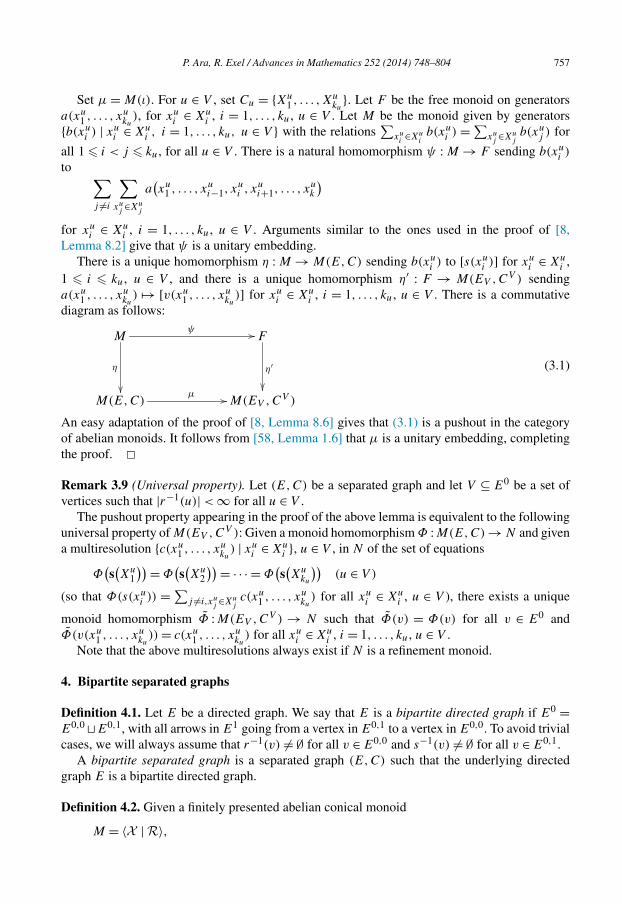
diagram as follows:
Mψ
η
F
η′
M(E,C)μ
M(EV ,CV )
(3.1)
An easy adaptation of the proof of [8, Lemma 8.6] gives that (3.1) is a pushout in the categoryof abelian monoids. It follows from [58, Lemma 1.6] that μ is a unitary embedding, completingthe proof. �Remark 3.9 (Universal property). Let (E,C) be a separated graph and let V ⊆ E0 be a set ofvertices such that |r−1(u)| < ∞ for all u ∈ V .
The pushout property appearing in the proof of the above lemma is equivalent to the followinguniversal property of M(EV ,CV ): Given a monoid homomorphism Φ :M(E,C) → N and givena multiresolution {c(xu
1 , . . . , xuku
) | xui ∈ Xu
i }, u ∈ V , in N of the set of equations
Φ(s(Xu
1
))= Φ(s(Xu
2
))= · · · = Φ(s(Xu
ku
))(u ∈ V )
(so that Φ(s(xui )) =∑j =i,xu
j ∈Xujc(xu
1 , . . . , xuku
) for all xui ∈ Xu
i , u ∈ V ), there exists a unique
monoid homomorphism Φ :M(EV ,CV ) → N such that Φ(v) = Φ(v) for all v ∈ E0 andΦ(v(xu
1 , . . . , xuku
)) = c(xu1 , . . . , xu
ku) for all xu
i ∈ Xui , i = 1, . . . , ku, u ∈ V .
Note that the above multiresolutions always exist if N is a refinement monoid.
4. Bipartite separated graphs
Definition 4.1. Let E be a directed graph. We say that E is a bipartite directed graph if E0 =E0,0 �E0,1, with all arrows in E1 going from a vertex in E0,1 to a vertex in E0,0. To avoid trivialcases, we will always assume that r−1(v) = ∅ for all v ∈ E0,0 and s−1(v) = ∅ for all v ∈ E0,1.
A bipartite separated graph is a separated graph (E,C) such that the underlying directedgraph E is a bipartite directed graph.
Definition 4.2. Given a finitely presented abelian conical monoid
M = 〈X | R〉,
758 P. Ara, R. Exel / Advances in Mathematics 252 (2014) 748–804
where X is a finite set of generators a1, . . . , an and R is a finite set of relations r1, . . . , rm of theform
rj :n∑
i=1
rjiai =n∑
i=1
sjiai, (4.1)
where rji and sji are non-negative integers satisfying∑n
i=1 rji > 0 and∑n
i=1 sji > 0 for all j ,and∑m
j=1(rji + sji) > 0 for all i, we may associate to it a finite bipartite separated graph (E,C)
such that s−1(v) = ∅ for all v ∈ E0,0 and r−1(v) = ∅ for all v ∈ E0,1, as follows (cf. [8, Propo-sition 4.4]):
E0 = E0,0 � E0,1, with E0,0 =R, E0,1 =X .
For rj ∈ R given by (4.1), we set Crj= {Xj ,Yj }, where Xj has exactly rji arrows from ai
to rj , for i = 1, . . . , n, and Yj has exactly sji arrows from ai to rj , for i = 1, . . . , n, so thatr−1(rj ) = Xj � Yj . Then E1 =⊔m
j=1 r−1(rj ). We have an isomorphism M(E,C) ∼= M [8,Proposition 4.4].
Note that there is a bijective correspondence between the finite bipartite separated graphs(E,C) satisfying the conditions in Definition 4.1 such that |Cv| = 2 for all v ∈ E0,0 and thefinite presentations of abelian conical monoids as above. Also, recall that every finitely generatedabelian semigroup is finitely presented, by Redei’s Theorem (see [30] for a very simple proof),so that we can apply the above process to any finitely generated abelian conical monoid. (Ofcourse, the finite bipartite separated graph will depend on the finite presentation, not just on themonoid.)
It is useful to introduce the following terminology:
Definition 4.3. Let M be an abelian conical monoid. A refinement of M is an abelian conicalmonoid N , together with a monoid homomorphism ι :M → N such that:
(a) ι is a unitary embedding.(b) N is a refinement monoid.(c) For each refinement monoid P and each monoid homomorphism ψ :M → P there is a
monoid homomorphism ψ :N → P such that ψ = ψ ◦ ι.
Construction 4.4. (a) Let (E,C) be a finite bipartite separated graph. We define a nested se-quence of finite separated graphs (Fn,D
n) as follows. Set (F0,D0) = (E,C). Assume that a
nested sequence(F0,D
0)⊂ (F1,D1)⊂ · · · ⊂ (Fn,D
n)
has been constructed in such a way that for i = 1, . . . , n, we have F 0i =⊔i+1
j=0 F 0,j for some finite
sets F 0,j and F 1i =⊔i
j=0 F 1,,j , with s(F 1,j ) = F 0,j+1 and r(F 1,j ) = F 0,j for j = 1, . . . , i. Wecan think of (Fn,D
n) as a union of n bipartite separated graphs. Assume that condition (∗)
for (Fn,Dn) holds at all vertices in
⊔n−1j=0 F 0,j . Set Vn = F 0,n, and let (Fn+1,D
n+1) be the
multiresolution of (Fn,Dn) at Vn. Then F 0
n+1 = F 0n � F 0,n+2 =⊔n+2
j=1 F 0,j and F 1n+1 = F 1
n �F
1,n+1n+1 =⊔n+1
j=0 F 1,j , with s(F 1,n+1) = F 0,n+2 and r(F 1,n+1) = s(F 1,n) = F 0,n+1. Moreover,
by Lemma 3.6, the separated graph (Fn+1,Dn+1) satisfies condition (∗) at all the vertices in⊔n
F 0,j .
j=0
P. Ara, R. Exel / Advances in Mathematics 252 (2014) 748–804 759
(b) Let
(F∞,D∞)= ∞⋃
n=0
(Fn,D
n).
Observe that (F∞,D∞) is the direct limit of the sequence {(Fn,Dn)} in the category FSGr de-
fined in [8, Definition 8.4]. Since the functor M : FSGr → Mon is continuous (see [8, 8.4, 4.1]),it follows that M(F∞,D∞) = lim−→M(Fn,D
n). Since (F∞,D∞) clearly satisfies condition (∗)
at all its vertices, it follows from [8, Proposition 5.9] that M(F∞,D∞) is a refinement monoid.Moreover, since all maps M(Fn,D
n) → M(Fn+1,Dn+1) are unitary embeddings by Lemma 3.6,
it follows that the map M(E,C) → M(F∞,D∞) is a unitary embedding. Finally, condition (c)in Definition 4.3 follows from Remark 3.9. Hence, we have that M(E,C) → M(F∞,D∞) is arefinement of M(E,C). We call (F∞,D∞) the complete multiresolution of (E,C).
(c) We define a canonical sequence (En,Cn) of finite bipartite separated graphs as follows:
(1) Set (E0,C0) = (E,C).
(2) E0,0n = F 0,n, E
0,1n = F 0,n+1, and E1
n = F 1,n. Moreover Cnv = Dn
v for all v ∈ E0,0n and
Cnv = ∅ for all v ∈ E
0,1n .
We call the sequence {(En,Cn)}n�0 the canonical sequence of bipartite separated graphs asso-
ciated to (E,C).
Lemma 4.5. Let (E,C) be a finite bipartite separated graph, let (En,Cn) be the canonical
sequence of bipartite separated graphs associated to (E,C), and let (F∞,D∞) be the completemultiresolution of (E,C). Then the following properties hold:
(a) For each n� 0, there is a natural isomorphism
ϕn :M(En+1,C
n+1)→ M((En)Vn,
(Cn)Vn),
where Vn = E0,0n = F 0,n.
(b) For each n� 0, there is a canonical unitary embedding
ιn :M(En,C
n)→ M
(En+1,C
n+1).(c) The canonical inclusion jn : (En,C
n) → (Fn,Dn) induces an isomorphism
M(jn) :M(En,C
n)→ M
(Fn,D
n).
(d) We have M(F∞,D∞) ∼= lim−→(M(En,Cn), ιn). Consequently, the natural map M(E,C) →
lim−→(M(En,Cn), ιn) is a refinement of M(E,C).
Proof. To simplify the notation, write EVn := (En)Vn and CVn = (Cn)Vn .(a) Define ϕn :M(En+1,C
n+1) → M(EVn,CVn) by ϕn(av) = av for v ∈ E0
n+1. Conversely,define ψn :M(EVn,C
Vn) → M(En+1,Cn+1) by ψn(av) = av for v ∈ E0
n+1 ⊂ E0Vn
and ψn(av) =s(X) for X ∈ Cv if v ∈ E
0,0n . We have to show that ψn is a well-defined monoid homomorphism.
There are no relations at the vertices at E0,1n+1, both in M(En+1,C
n+1) and in M(EVn,CVn),
because these vertices are sources in both graphs. It is clear that the relations at vertices v in

760 P. Ara, R. Exel / Advances in Mathematics 252 (2014) 748–804
E0,0n+1 are preserved by ψn, because Cn+1
v = CVnv for these vertices. For a vertex v ∈ E
0,0n , take
X,Y ∈ Cv . Setting Cv = {X1, . . . ,Xs}, there are 1 � p,q � s such that X = Xp and Y = Xq . InM(En+1,C
n+1), we have
s(Xp) =∑
xp∈Xp
s(xp) =∑
(x1,...,xs )∈∏si=1 Xi
v(x1, . . . , xs) =∑
xq∈Xq
s(xq) = s(Xq). (4.2)
Hence s(X) = s(Y ) for all X,Y ∈ Cv , which shows that ψn is well-defined. Clearly ϕn and ψn
are mutually inverse, so we get that ϕn is an isomorphism.(b) By Lemma 3.8, the natural map M(ιVn) :M(En,C
n) → M(EVn,CVn) is a unitary embed-
ding. Hence the map ιn = ϕ−1n ◦M(ιVn) :M(En,C
n) → M(En+1,Cn+1) is a unitary embedding.
(c) We use induction on n. For n = 0, we have (E0,C0) = (F0,D
0). Assume that, for somen� 0, the natural map jn : (En,C
n) → (Fn,Dn) induces an isomorphism M(jn) :M(En,C
n) →M(Fn,D
n). Since (Fn+1,Dn+1) = ((Fn)Vn, (D
n)Vn), we get an isomorphism M(EVn,CVn) →
M(Fn+1,Dn+1) extending M(jn). Now we have the following commutative diagram:
M(En,Cn)
M(ιVn )−−−−→ M(EVn,CVn)
ϕn←−−−− M(En+1,Cn+1)
M(jn)
⏐⏐� ∼=⏐⏐� ⏐⏐�M(jn+1)
M(Fn,Dn) −−−−→ M(Fn+1,D
n+1)id−−−−→ M(Fn+1,D
n+1)
(4.3)
Since ϕn is an isomorphism by (a), we get that M(jn+1) is also an isomorphism.(d) Write R = lim−→(M(ιn), ιn). We have from (c) a commutative diagram
M(E0,C0)
ι0
id
M(E1,C1)
ι1
M(j1) ∼=
M(E2,C2)
M(j2) ∼=
R
M(F0,D0) M(F1,D
1) M(F2,D2) M(F∞,D∞)
such that all the vertical maps M(jn) :M(En,Cn) → M(Fn,D
n) are isomorphisms, so we getan isomorphism R → M(F∞,D∞). This shows the result. �
Given a finite presentation 〈X | R〉 of a finitely presented abelian conical monoid M as inDefinition 4.2, we can associate to it the refinement monoid
R(X |R) = M(F∞,D∞),
where (F∞,D∞) is the complete multiresolution of the bipartite separated graph associated tothe presentation 〈X | R〉. Observe that this construction depends strongly on the presentation,not just the monoid M . For instance, we may consider two different presentations 〈a, b | a = a,
b = b〉 and 〈a, b | a + b = a + b〉 of the free abelian monoid on two generators F . In the firstpresentation the resulting R is just F . For the second presentation, the corresponding refinementmonoid R is atomless, and is isomorphic to the monoid V(K[G]), where G is the lamplightergroup, see Example 9.7.

P. Ara, R. Exel / Advances in Mathematics 252 (2014) 748–804 761
If we consider the standard presentation
M(E) =⟨av
∣∣∣ av =∑
e∈r−1(v)
as(e)
(v ∈ E0)⟩
of a graph monoid M(E) associated to a non-separated finite graph E, then it can be shown thatR = M(E). Since R is a refinement monoid, we obtain an alternative proof of [10, Proposi-tion 4.4] for finite graphs.
5. The main construction
This section contains our main construction on algebras. Let (E,C) be a finite bipartite sepa-rated graph, with r(E1) = E0,0 and s(E1) = E0,1. Let {(En,C
n)}n�0 be the canonical sequenceof bipartite separated graphs associated to it (see Definition 4.4(c)), and let Bn be the commuta-tive, finite dimensional subalgebra of L(En,C
n) generated by E0n . Here L(En,C
n) stands for theLeavitt path ∗-algebra of the separated graph (En,C
n) over a fixed field with involution (K,∗).
Theorem 5.1. With the above notation, for each n� 0, there exists a surjective ∗-algebra homo-morphism
φn :L(En,C
n)� L(En+1,C
n+1).Moreover, the following properties hold:
(a) ker(φn) is the ideal In of L(En,Cn) generated by all the commutators [ee∗, ff ∗], with
e,f ∈ E1n , so that L(En+1,C
n+1) ∼= L(En,Cn)/In.
(b) The restriction of φn to Bn defines an injective homomorphism from Bn into Bn+1.(c) There is a commutative diagram
M(En,Cn)
ιn−−−−→ M(En+1,Cn+1)
∼=⏐⏐� ⏐⏐�∼=
V(L(En,Cn))
V(φn)−−−−→ V(L(En+1,Cn+1))
(5.1)
where the vertical maps are the canonical maps, which are isomorphisms by [8, Theo-rem 4.3].
Proof. Set An = L(En,Cn). Define φn :An → An+1 on vertices u ∈ E
0,0n by the formula
φn(u) =∑
(x1,...,xku )∈∏kui=1 Xu
i
v(x1, . . . , xku),
where Cu = {Xu1 , . . . ,Xu
ku}, and by φn(w) = w for all w ∈ E
0,1n . For an arrow xi ∈ Xu
i , define
φn(xi) =∑
xj ∈Xuj ,j =i
(αxi (x1, . . . , xi , . . . , xku)
)∗,
where αxi (x1, . . . , xi , . . . , xku) = αxi (x1, . . . , xi−1, xi+1, . . . , xku). We have to show that thedefining relations of L(En,C
n) are preserved by φn. It is easily checked that (V) and (E) are

762 P. Ara, R. Exel / Advances in Mathematics 252 (2014) 748–804
preserved by φn. To see that (SCK1) is preserved by φn, take u ∈ E0,0n and xi, x
′i ∈ Xu
i forsome i. Observe that
φn(xi)∗φn
(x′i
)= ∑xj ,yj ∈Xu
j ,j =i
αxi (x1, . . . , xi , . . . , xku)αx′i(y1, . . . , x
′i , . . . , yku
)∗.
If xi = x′i , then v(x1, . . . , xi, . . . , xku)v(y1, . . . , x
′i , . . . , yku) = 0 for all xj , yj ∈ Xu
j , j = i, and soφn(xi)
∗φn(x′i ) = 0. If xi = x′
i then v(x1, . . . , xi, . . . , xku)v(y1, . . . , xi, . . . , yku) = 0 except whenxj = yj for all j = i, and, hence recalling that X(xi) ∈ Cn+1
s(xi ), we get
φn(xi)∗φn
(x′i
)= ∑xj ∈Xu
j ,j =i
αxi (x1, . . . , xi , . . . , xku)αxi (x1, . . . , xi , . . . , xku)
∗
=∑
z∈X(xi)
zz∗ = s(xi),
as desired. Finally we check that (SCK2) is also preserved by φn. Take u ∈ E0,0n and Xu
i ∈ Cnu .
Then ∑xi∈Xu
i
φn(xi)φn(xi)∗ =∑
xi∈Xui
∑xj ∈Xu
j ,j =i
αxi (x1, . . . , xi , . . . , xku)∗αxi (x1, . . . , xi , . . . , xku)
=∑
(x1,...,xku )∈∏kuj=1 Xu
j
v(x1, . . . , xku) = φn(u),
as wanted.To check surjectivity, it is enough to check that all vertices and edges in En+1 belong to the
image of φn. Clearly, w ∈ φn(An) for all w ∈ E0,0n+1. Now take xi ∈ Xu
i , for i = 1,2, . . . , ku. Wehave
φn(xi)φn(xi)∗ =
∑yj ∈Xu
j ,j =i
v(y1, . . . , xi, . . . , yku). (5.2)
Therefore, we get
v(x1, x2, . . . , xku) = φn
((x1x
∗1
)(x2x
∗2
) · · · (xkux∗ku
)), (5.3)
showing that v(x1, x2, . . . , xn) ∈ φn(An). Moreover, we get
αxi (x1, . . . , xi , . . . , xku)∗ = v(x1, . . . , xku)φn(xi), (5.4)
which, together with (5.3) gives that αxi (x1, . . . , xi , . . . , xku) ∈ φn(An). This concludes the proofthat φn is surjective.
We now proceed to show (a), (b), (c).(a) It follows from (5.2) that {φn(ee
∗) | e ∈ E1n} is a family of commuting projections in
L(En+1,Cn+1). Therefore all commutators [ee∗, ff ∗] are contained in the kernel of φn, and we
obtain an induced surjective map φn :An/In → An+1. We define a map γn :An+1 → An/In byγn(w) = w for w ∈ E
0,0n+1, and
γn
(v(x1, . . . , xku)
)= (x1x∗1
)(x2x
∗2
) · · · (xkux∗ku
),
γn
(αxi (x1, . . . , xi , . . . , xku)
)= x∗(x1x∗)(x2x
∗) · · · (xkux∗ )
i 1 2 ku
P. Ara, R. Exel / Advances in Mathematics 252 (2014) 748–804 763
for (xj ) ∈∏ku
j=1 Xj . Using the commutativity in An/In of the set of projections {ee∗ | e ∈ E1n},
and the defining relations of L(En,Cn), it is easy to check that the defining relations of
An+1 = L(En+1,Cn+1) are preserved by γn. Clearly, γn is the inverse of φn, and so we get
that ker(φn) = In.(b) This follows from the definition of φn.(c) Denote by τn :M(En,C
n) → V(An) the natural map sending av to [v], for v ∈ E0n . This
map is an isomorphism by [8, Theorem 4.3]. Recall that ιn = ϕ−1n ◦ M(ιVn) = ψn ◦ M(ιVn) has
been defined in the proof of Lemma 4.5(b).If w ∈ E
0,1n then (τn+1 ◦ ιn)(aw) = [w] = (V(φn) ◦ τn)(aw). If u ∈ E
0,0n , then it follows from
the definition of ψn, formula (4.2) and the definition of φn that
(τn+1 ◦ ιn)(au) =∑
(xj )∈∏kuj=1 Xu
j
[v(x1, . . . , xku)
]= (V(φn) ◦ τn
)(au),
so that we get the commutativity of the diagram (5.1). �We now study in more detail the relationship between the different layers. To simplify the
notation, we will write Dn = F 0,n = E0,0n for all n� 0.
Note that, for n� 2 we have a surjective map rn :Dn → Dn−2 given by rn(v(x1, . . . , xku))=u,where u ∈ Dn−2 and xi ∈ Xu
i , and where, as usual, Cu = {Xu1 , . . . ,Xu
ku}. For n = 2m, we
thus obtain a surjective map r2m = r2 ◦ r4 ◦ · · · ◦ r2m :D2m → D0. Similarly, we have a mapr2m+1 = r3 ◦ r5 ◦ · · · ◦ r2m+1 :D2m+1 → D1. We call r(v) the root of v. Observe that we have
D2n =⊔
v∈D0
r−12n (v); D2n+1 =
⊔v∈D1
r−12n+1(v). (5.5)
Lemma 5.2.
(1) For all n� 1 and v ∈ D2n we have |s−1(v)| = |Cv| = |Cr2n(v)|.(2) For all n� 0 and w ∈ D2n+1 we have |s−1(w)| = |Cw| = |Cr2n+1(w)|.
Proof. (1) By induction, it suffices to show that |s−1(v)| = |Cv| = |Cr2n(v)| for every v ∈ D2n,n� 1. Let v ∈ D2n, n� 1, and write v = v(x1, . . . , xku), where xi ∈ Xu
i and Cu = {Xu1 , . . . ,Xu
ku}.
Note that s−1(v) has exactly ku elements, namely
αx1(x2, . . . , xku), . . . , αxku (x1, . . . , xku−1).
Thus |s−1(v)| = ku = |Cu| = |Cr2n(v)|. On the other hand, by definition Cv = {X(y) | y ∈s−1E2n−1
(v)}, so that |Cv| = |s−1(v)| = |Cu|, as desired.(2) This is proved exactly as in (1). �
Remark 5.3. Fix an enumeration {Xu1 , . . . ,Xu
ku} for the elements of Cu, where u ∈ D0 = E0,0.
This gives an enumeration of the elements in s−1(v) for v ∈ r−12 (u). Indeed, for such an ele-
ment v we have v = v(x1, . . . , xkn), with xi ∈ Xui , and we can set zi = αxi (x1, . . . , xi , . . . , xku),
so that we obtain the enumeration {z1, . . . , zku} of s−1(v). This in turn gives an enumerationof the elements of the set Cv , namely Cv = {Xv
1 , . . . ,Xvku
}, where Xvi = X(zi) for all i. Obvi-
ously this translates to all the vertices v ∈ D2n, so that we obtain canonical enumerations of theelements of s−1(v) and of the elements of Cv .

764 P. Ara, R. Exel / Advances in Mathematics 252 (2014) 748–804
Define Φn = φn−1 ◦ · · · ◦ φ0 :L(E,C) → L(En,Cn).
Lemma 5.4. Let u ∈ D0 and set Cu = {Xu1 , . . . ,Xu
ku}. For each n� 1 and each i with 1 � i � ku,
there exists a partition
r−12n (u) =
⊔xi∈Xu
i
Z2n(xi),
such that, for each xi ∈ Xui , we have
Φ2n(xi) =∑
v∈Z2n(xi )
∑x∈Xv
i
x, (5.6)
where the enumeration of the elements in Cv , v ∈ D2n, is the canonical one described in Re-mark 5.3.
Proof. We first prove the case n = 1. Observe that φ0(xi) =∑y∈X(xi)y∗. The elements y ∈
X(xi) are of the form αxi (x1, . . . , xi , . . . , xku), and we set
Z2(xi) = {s(y)∣∣ y ∈ X(xi)
}= {v(x1, . . . , xi, . . . , xku)∣∣ xj ∈ Xu
j , j = i}.
Note that s(y) = s(y′) for y, y′ ∈ X(xi) with y = y′. Observe that we get a partition
r−12 (u) =
⊔xi∈Xu
i
Z2(xi).
Let v = v(x1, . . . , xi, . . . , xku) ∈ Z2(xi). Then in the canonical enumeration of the elements ofs−1(v), say {z1, . . . , zku}, the element αxi (x1, . . . , xi , . . . , xku) corresponds to zi , and there is noother element of X(xi) having source equal to v. The corresponding element X(y) = X(zi) ofCv is the element labeled as Xv
i (see Remark 5.3). Therefore we get
Φ2(xi) = φ1
( ∑y∈X(xi)
y∗)
=∑
y∈X(xi)
∑x∈X(y)
x =∑
v∈Z2(xi )
∑x∈Xv
i
x.
Assume now that n� 1 and that (5.6) holds. Note that
φ2n
(Φ2n(xi)
)= ∑v∈Z2n(xi )
∑x′i∈Xv
i
∑y∈X(x′
i )
y∗. (5.7)
Observe that⊔
x′i∈Xv
i{s(y) | y ∈ X(x′
i )} = r−12n+2(v), and that s(y) = s(y′) for y = y′ and y, y′ ∈⋃
v∈Z2n(xi )
⋃x′i∈Xv
iX(x′
i ). Set
Z2n+2(xi) =⊔
v∈Z2n(xi )
r−12n+2(v) = r−1
2n+2
(Z2n(xi)
).
Clearly we get a partition r−12n+2(u) =⊔xi∈Xu
iZ2n+2(xi). Moreover, arguing as in the case n = 1
we get
Φ2n+2(xi) = φ2n+1
( ∑v∈Z2n(xi )
∑x′i∈Xv
i
∑y∈X(x′
i )
y∗)
=∑
v∈Z2n(xi )
∑x′i∈Xv
i
∑y∈X(x′
i )
∑x∈X(y)
x =∑
v′∈Z2n+2(xi )
∑x∈Xv′
i
x,
completing the induction step. �
P. Ara, R. Exel / Advances in Mathematics 252 (2014) 748–804 765
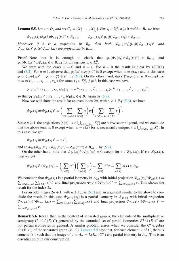
Lemma 5.5. Let u ∈ D0 and set Cu = {Xu1 , . . . ,Xu
ku}. For xi ∈ Xu
i , n� 0 and b ∈ Bn we have
Φn+1(xi)φn(b)Φn+1(xi)∗ ∈ Bn+1, Φn+1(xi)
∗φn(b)Φn+1(xi) ∈ Bn+1.
Moreover, if b is a projection in Bn, then both Φn+1(xi)φn(b)Φn+1(xi)∗ and
Φn+1(xi)∗φn(b)Φn+1(xi) are projections in Bn+1.
Proof. Note that it is enough to check that φn(Φn(xi)wΦn(xi)∗) ∈ Bn+1 and
φn(Φn(xi)∗wΦn(xi)) ∈ Bn+1 for all vertices w ∈ E0
n .We start with the cases n = 0 and n = 1. For n = 0 the result is clear by (SCK1)
and (5.2). For n = 1, observe that φ0(xi)wφ0(xi)∗ is 0 except when w = s(xi) and in this case
φ0(xi)wφ(xi)∗ = φ0(xix
∗i ) ∈ B1 by (5.2). On the other hand, φ0(xi)
∗wφ0(xi) is 0 except forw = v(x1, . . . , xi, . . . , xku) for some xj ∈ Xu
j , j = i. In this case we have
φ0(xi)∗v(x1, . . . , xku)φ0(xi) = αxi (x1, . . . , xi , . . . , xku)α
xi (x1, . . . , xi , . . . , xku)∗,
so that φ1(φ0(xi)∗v(x1, . . . , xku)φ0(xi)) ∈ B2 again by (5.2).
Now we will show the result for an even index 2n, with n� 1. By (5.6), we have
Φ2n(xi)wΦ2n(xi)∗ =( ∑
v∈Z2n(xi )
∑x∈Xv
i
x
)w
( ∑v∈Z2n(xi )
∑x∈Xv
i
x
)∗.
Since n� 1, the projections {s(x) | x ∈⋃v∈Z2n(xi )Xv
i } are pairwise orthogonal, and we concludethat the above term is 0 except when w = s(x) for a, necessarily unique, x ∈⋃v∈Z2n(xi )
Xvi . In
this case, we get
Φ2n(xi)wΦ2n(xi)∗ = xx∗,
and so φ2n(Φ2n(xi)wΦ2n(xi)∗) = φ2n(xx∗) ∈ B2n+1 by (5.2).
On the other hand, note that Φ2n(xi)∗vΦ2n(xi) = 0 except for v ∈ Z2n(xi). If v ∈ Z2n(xi),
then we get
Φ2n(xi)∗vΦ2n(xi) =
( ∑x∈Xv
i
x∗)( ∑
y∈Xvi
y
)=∑x∈Xv
i
x∗x =∑x∈Xv
i
s(x) ∈ B2n.
We conclude that Φ2n(xi) is a partial isometry in A2n with initial projection Φ2n(xi)∗Φ2n(xi) =∑
v∈Z2n(xi )
∑x∈Xv
is(x) and final projection Φ2n(xi)Φ2n(xi)
∗ =∑v∈Z2n(xi )v. This shows the
result for the index 2n.For an odd integer 2n + 1, with n� 1, use (5.7) and an argument similar to the above to con-
clude the result. In this case Φ2n+1(xi) is a partial isometry in A2n+1 with initial projectionΦ2n+1(xi)
∗Φ2n+1(xi) =∑v∈Z2n(xi )
∑x∈Xv
is(x) and final projection Φ2n+1(xi)Φ2n+1(xi)
∗ =∑v∈Z2n+2(xi )
v. �Remark 5.6. Recall that, in the context of separated graphs, the elements of the multiplicativesemigroup U of L(E,C) generated by the canonical set of partial isometries E1 ∪ (E1)∗ arenot partial isometries in general. A similar problem arises when we consider the C∗-algebraC∗(E,C) of the separated graph (E,C). Lemma 5.5 says that, for each element u of U , there issome m� 1 such that the image of u in Am = L(Em,Cm) is a partial isometry in Am. This is anessential point in our construction.
766 P. Ara, R. Exel / Advances in Mathematics 252 (2014) 748–804
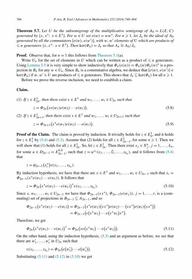
Theorem 5.7. Let U be the subsemigroup of the multiplicative semigroup of A0 = L(E,C)
generated by {x, x∗: x ∈ E1}. For w ∈ U set e(w) = ww∗. For n � 1, let Jn be the ideal of A0generated by all the commutators [e(w), e(w′)], with w,w′ elements of U which are products of� n generators {x, x∗: x ∈ E1}. Then ker(Φn) = Jn so that An
∼= A0/Jn.
Proof. Observe that, for n = 1 this follows from Theorem 5.1(a).Write Un for the set of elements in U which can be written as a product of � n generators.
Using Lemma 5.5 it is very simple to show inductively that Φn(e(w)) = Φn(w)Φn(w)∗ is a pro-jection in Bn for any w ∈ Un. Since Bn is a commutative algebra, we deduce that [e(w), e(w′)] ∈ker(Φn) if w,w′ ∈ U are products of � n generators. This shows that Jn ⊆ ker(Φn) for all n� 1.
Before we prove the reverse inclusion, we need to establish a claim.
Claim.
(1) If z ∈ E12n, then there exist x ∈ E1 and w1, . . . ,wt ∈ U2n such that
z = Φ2n
(xe(w1)e(w2) · · · e(wt )
). (5.8)
(2) If z ∈ E12n+1, then there exist x ∈ E1 and w1, . . . ,wt ∈ U2n+1 such that
z = Φ2n+1(x∗e(w1)e(w2) · · · e(wt )
). (5.9)
Proof of the Claim. The claim is proved by induction. It trivially holds for z ∈ E10 , and it holds
for z ∈ E11 by (5.4) and (5.3). Assume that (2) holds for all z ∈ E1
2n−1, for some n � 1. Then wewill show that (1) holds for all z ∈ E1
2n. So, let z ∈ E12n. Then there exist xj ∈ Xu
j , j = 1, . . . , ku,
for some u ∈ D2n−1 = E0,02n−1, such that z = αxi (x1, . . . , xi , . . . , xku), and it follows from (5.4)
that
z = φ2n−1(x∗i
)v(x1, . . . , xku).
By induction hypothesis, we have that there are x ∈ E1 and w1, . . . ,wt ∈ U2n−1 such that xi =Φ2n−1(x
∗e(w1) · · · e(wt )). It follows that
z = Φ2n
(x∗e(w1) · · · e(wt )
)∗v(x1, . . . , xku). (5.10)
Since x,w1, . . . ,wt ∈ U2n−1 we have that Φ2n−1(xx∗), Φ2n−1(e(wj )), j = 1, . . . , t , is a (com-muting) set of projections in B2n−1 ⊆ A2n−1, and so
Φ2n−1(x∗e(w1) · · · e(wt )
)= Φ2n−1(x∗e(w1)
(xx∗)e(w2) · · · (xx∗)e(wt )
(xx∗))
= Φ2n−1(e(x∗w1) · · · e(x∗wt
)x∗).
Therefore, we get
Φ2n
(x∗e(w1) · · · e(wt )
)∗ = Φ2n
(xe(x∗wt
) · · · e(x∗w1))
. (5.11)
On the other hand, using the induction hypothesis, (5.3) and an argument as before, we see thatthere are w′
1, . . . ,w′s in U2n such that
v(x1, . . . , xku) = Φ2n
(e(w′
1
) · · · e(w′s
)). (5.12)
Substituting (5.11) and (5.12) in (5.10) we get

P. Ara, R. Exel / Advances in Mathematics 252 (2014) 748–804 767
z = Φ2n
(xe(x∗wt
) · · · e(x∗w1)e(w′
1
) · · · e(w′s
)),
showing (5.8). A similar argument shows that (1) implies (2) for the index 2n+1. This concludesthe proof of the Claim. �
Now we follow with the proof of the theorem. We show the reverse inclusion ker(Φm) ⊆ Jm byinduction on m. For m = 1, the result follows from Theorem 5.1(a). Assume that the result holdsfor some m � 1 and let us show that it also holds for m + 1. Observe that, by Theorem 5.1(a),kerΦm+1/kerΦm is the ideal of Am generated by [zz∗, (z′)(z′)∗], where z, z′ ∈ E1
m. Assume firstthat m = 2n for some n � 0 and that z, z′ ∈ E1
2n. By the first part of the Claim, there exist thenx, x′ ∈ E1 and w1, . . . ,wt ,w
′1, . . . ,w
′t ′ ∈ U2n such that
z = Φ2n
(xe(w1)e(w2) · · · e(wt )
), z′ = Φ2n
(x′e(w′
1
)e(w′
2
) · · · e(w′t ′))
.
Since kerΦ2n = J2n by induction hypothesis, and J2n ⊆ J2n+1, it is enough to check that[xe(w1) · · · e(wt )e(wt )
∗ · · · e(w1)∗x∗, x′e
(w′
1
) · · · e(w′t ′)e(w′
t ′)∗ · · · e(w′
1
)∗(x′)∗] ∈ J2n+1.
We have[xe(w1) · · · e(wt )e(wt )
∗ · · · e(w1)∗x∗ + J2n,
x′e(w′
1
) · · · e(w′t ′)e(w′
t ′)∗ · · · e(w′
1
)∗(x′)∗ + J2n
]= [xe(w1) · · · e(wt )x
∗ + J2n, x′e(w′
1
) · · · e(w′t ′)(
x′)∗ + J2n
]= [xe(w1)
(x∗x)e(w2) · · · (x∗x
)e(wt )x
∗ + J2n,
x′e(w′
1
)(x′)∗x′e
(w′
2
) · · · (x′)∗x′e(w′
t ′)(
x′)∗ + J2n
]= [e(xw1)e(xw2) · · · e(xwt ) + J2n, e
(x′w′
1
)e(x′w′
2
) · · · e(x′w′t ′)+ J2n
]⊆∑i,j
A0[e(xwi), e
(x′w′
j
)]A0 + J2n ⊆ J2n+1,
where we have used the Leibnitz rule (i.e. [xy, z] = [x, z]y + x[y, z]) for the first containment.A similar argument, using part (2) of the Claim instead of part (1), gives the proof of the inductivestep for m = 2n + 1. This completes the proof of the theorem. �
Write A∞ = lim−→An, and B∞ = lim−→Bn. We have a commutative diagram as follows:
B0 B1 B2 B∞
A0φ0
A1φ1
A2 A∞All the maps Bn → Bn+1 are injective and all the maps An → An+1 are surjective.
Notation 5.8. We write Lab(E,C) = A∞. Observe that, by Theorem 5.7, Lab(E,C) ∼=L(E,C)/J , where J =⋃∞
Jn is the ideal generated by all the commutators [e(w), e(w′)],
n=1
768 P. Ara, R. Exel / Advances in Mathematics 252 (2014) 748–804
with w,w′ ∈ U . If we use in the above construction the full graph C∗-algebras C∗(En,Cn) in-
stead of the Leavitt path algebras L(En,Cn), we obtain in the limit a certain C∗-algebra, that we
denote by O(E,C), in analogy with the notation introduced in [5].
Corollary 5.9. We have V(Lab(E,C)) ∼= lim−→(M(En,Cn), ιn) ∼= M(F∞,D∞). Consequently the
natural map M(E,C) → V(Lab(E,C)) is a refinement of M(E,C).
Proof. This follows immediately from the continuity of the functor V , Theorem 5.1(c) andLemma 4.5(d). �Remark 5.10. Assume that K = C, the complex field. Then the commutative ∗-algebra B∞is an algebraic direct limit of finite-dimensional commutative C∗-algebras Bn, with injectivemaps φn|Bn :Bn → Bn+1. Since each Bn sits as a C∗-subalgebra of C∗(En,C
n) (cf. [7, Theo-rem 3.8(1)]), it follows that the C∗-completion B0 of B∞ sits as a C∗-subalgebra of O(E,C).
Recall the following definition from [24]. (The definition has been conveniently modified towork in the purely algebraic situation as well as in the C∗-context.)
Definition 5.11. A set S of partial isometries in a ∗-algebra A is said to be tame if every elementof U = 〈S ∪ S∗〉, the multiplicative semigroup generated by S ∪ S∗, is a partial isometry, andthe set {e(u) | u ∈ U} of final projections of the elements of U is a commuting set of projectionsof A.
We are now ready to show that Lab(E,C) is the universal algebra generated by a tame set ofpartial isometries x, for x ∈ E1 satisfying the defining relations of L(E,C), which can be restatedcompletely in terms of the elements in E1 ∪ (E1)∗, indeed in terms of the final projections e(u)
of these elements, as follows:
(PI1) e(x)e(y) = δx,ye(x), for x, y ∈ X, X ∈ C.(PI2) e(x∗) = e(y∗) if x, y ∈ E1 and s(x) = s(y).(PI3)
∑x∈X e(x) =∑y∈Y e(y) for all X,Y ∈ Cv , v ∈ E0,0.
For w ∈ E0,1 and x ∈ E1 with s(x) = w, denote the projection e(x∗) by pw . Similarly, forv ∈ E0,0, denote by pv the projection corresponding to
∑x∈X e(x), for X ∈ Cv . (Note that these
projections are well-defined by (PI1)–(PI3).)
(PI4) pvpv′ = 0 for every pair v, v′ of different vertices in E0, and∑
v∈E0 pv = 1.
Note that the condition∑
v∈E0 pv = 1 can be deduced from the other conditions, because E
is a finite graph. It is easily seen that for a finite bipartite separated graph satisfying our standingassumptions that s(E1) = E0,1 and r(E1) = E0,0, the algebra L(E,C) is just the universal al-gebra generated by a set of partial isometries x ∈ E1 subject to the above relations (PI1)–(PI4).A similar statement holds for the full graph C∗-algebra C∗(E,C).
Theorem 5.12. The algebra Lab(E,C) (respectively, the C∗-algebra O(E,C)) is the universal∗-algebra (respectively, universal C∗-algebra) generated by a tame set of partial isometries {x |x ∈ E1} satisfying the relations (PI1)–(PI4).

P. Ara, R. Exel / Advances in Mathematics 252 (2014) 748–804 769
Proof. Let U be the multiplicative semigroup of L(E,C) generated by E1 ∪ (E1)∗, and let Un
be the set of those elements of U which can be written as a product of � n generators. ThenLab(E,C) = L(E,C)/J , where J =⋃∞
n=1 Jn and Jn is the ideal generated by the commutators[e(w), e(w′)], with w,w′ ∈ Un (Theorem 5.7). If w ∈ Un then it was observed in the proof ofTheorem 5.7 that e(w) is a projection in An = L(E,C)/Jn. It is rather easy to show, by inductionon n, that this implies that every element of Un is a partial isometry in L(E,C)/Jn. Denotingby u the image of u ∈ U through the canonical projection L(E,C) → Lab(E,C), we thus havethat all elements u are partial isometries and the final projections of these elements commutewith each other. It follows that {x | x ∈ E1} is a tame set of partial isometries in Lab(E,C).Since J is the ideal generated by all the commutators [e(w), e(w′)], with w,w′ ∈ U , it is clearthat Lab(E,C) is the universal algebra generated by a tame set of partial isometries satisfyingconditions (PI1)–(PI4), as claimed.
The same proof works for O(E,C). �By Stone duality [53], there is a zero-dimensional metrizable compact space Ω(E,C) such
that the Boolean algebra of projections in B∞ is isomorphic to the Boolean algebra of clopensubsets of Ω(E,C). A convenient way of describing this space is as follows. Consider thecommutative AF -algebra B0, which is the C∗-completion of the locally matricial algebra B∞(taking K = C). Then there is a unique zero-dimensional metrizable compact topological spaceΩ(E,C) such that B0 ∼= C(Ω(E,C)). Observe that we have a basis of clopen sets for thetopology of Ω(E,C) which is in bijective correspondence with the vertices of the graph F∞.Note that for any field K , the algebra B∞ is the algebra CK(Ω(E,C)) of continuous functionsf :Ω(E,C) → K , where K is endowed with the discrete topology, see [35, Corollaire 1].
We record for later use a fundamental property of the algebra B∞.
Proposition 5.13. The algebra B∞ is generated by all the projections e(w), for w ∈ U .
Proof. The algebra B∞ is generated by the images under the limit maps of the projectionsv ∈ Dn, for n � 0. Now if v ∈ D0 then it follows from (SCK2) that v is a sum of projec-tions e(x), for x ∈ X, X ∈ Cv . Similarly, (SCK1) gives that the projections in D1 are of theform e(x∗). Suppose now that v ∈ Dn+1 with n � 1. Then v = v(x1, . . . , xku), where xi ∈ Xu
i ,Cu = {Xu
1 , . . . ,Xuku
} and u ∈ Dn−1. Then it follows from either (5.8) or (5.9), and Eq. (5.3) thatv(x1, . . . , xku) is a product of projections of the form Φn(e(w)), where w ∈ Un. �6. Dynamical systems
Definition 6.1. Let G be a group with identity element 1. A partial representation of G on aunital K-algebra A is a map π :G → A such that π(1) = 1A and
π(g)π(h)π(h−1)= π(gh)π
(h−1), π
(g−1)π(g)π(h) = π
(g−1)π(gh)
for all g,h ∈ G. If G is a free group on a set X and |g| denotes the length of g ∈ G withrespect to X, we say that a partial representation π is semi-saturated in case π(ts) = π(t)π(s)
for all t, s ∈ G with |ts| = |t | + |s|.
Definition 6.2. Let G be a group and let B be an associative K-algebra (possibly without unit).A partial action of G on B consists of a family of two-sided ideals Dg of B (g ∈ G) and algebraisomorphisms αg :Dg−1 → Dg such that

770 P. Ara, R. Exel / Advances in Mathematics 252 (2014) 748–804
(i) D1 = B and α1 is the identity map on B;(ii) αh(Dh−1 ∩Dg) =Dh ∩Dhg ;
(iii) αg ◦ αh(x) = αgh(x) for each x ∈ α−1h (Dh ∩Dg−1).
Let (E,C) be a finite bipartite separated graph, with r(E1) = E0,0 and s(E1) = E0,1, as inDefinition 4.1. Throughout this section, we will denote by F the free group on the set E1 of edgesof E.
Proposition 6.3. The algebra Lab(E,C) is the universal ∗-algebra for semi-saturated partialrepresentations of F satisfying the relations (PI1)–(PI4). That is, there is a semi-saturated partialrepresentation π :F → Lab(E,C) sending each x ∈ E1 to the element x of Lab(E,C), and,moreover given any semi-saturated partial representation ρ of F on a unital ∗-algebra B suchthat the partial isometries ρ(x), x ∈ E1 � (E1)∗, satisfy relations (PI1)–(PI4), there is a unique∗-algebra homomorphism ϕ :Lab(E,C) → B such that ρ = ϕ ◦ π .
Proof. Since {x | x ∈ E1} is a tame set of partial isometries in Lab(E,C), it follows from[24, Proposition 5.4] that there exists a (unique) semi-saturated partial representation π :F →Lab(E,C) such that π(x) = x for all x ∈ E1.
The universality follows from Theorem 5.12, just as in [5, 2.4]. �Let π :G → A be a partial representation of a group G on a unital K-algebra A. Then the
elements εg = π(g)π(g−1) (g ∈ G) are commuting idempotents such that
π(g)εh = εghπ(g), εhπ(g) = π(g)εg−1h, (6.1)
see [20, page 1944]. Let B be the subalgebra of A generated by all the εg (g ∈ G), and for g ∈ G
set Dg = εgB. By [20, Lemma 6.5], the maps απg :Dg−1 →Dg (g ∈ G) given by
απg (b) = π(g)bπ(g)∗
are isomorphisms of K-algebras which determine a partial action απ of G on B.In the case where A = Lab(E,C) and π :F → Lab(E,C) is the partial representation de-
scribed in Proposition 6.3, we set εw = e(w) ∈ B∞, and we observe that, by Proposition 5.13,the algebra B generated by all the projections e(w) (w ∈ F) is precisely the commutative alge-bra B∞. It follows that Dw = B∞e(w), the ideal of B∞ generated by e(w).
As noted above, it follows that the maps
φw :B∞e(w∗)→ B∞e(w)
defined by φw(b) = π(w)bπ(w)∗, give a partial action of F on B∞, namely φ = απ .We now recall the notion of a crossed product by a partial action, see e.g. [20, Definition 1.2].
Definition 6.4. Given a partial action α of a group G on a K-algebra B, the crossed prod-uct B �α G is the set of all finite formal sums {∑g∈G agδg | ag ∈ Dg}, where δg are symbols.Addition is defined in the obvious way, and multiplication is determined by (agδg) · (bhδh) =αg(αg−1(ag)bh)δgh.
Note that, given a partial action of G on a unital K-algebra B, we have a partial representationG → B�α G, defined by g �→ 1gδg (see [20, Lemma 6.2]).
We need a further definition.

P. Ara, R. Exel / Advances in Mathematics 252 (2014) 748–804 771
Definition 6.5. A partial (E,C)-action on a unital commutative ∗-algebra B consists of a collec-tion of projections {e(u) | u ∈ E1 ∪ (E1)∗} satisfying the conditions (PI1)–(PI4), together with acollection of ∗-algebra isomorphisms αx : e(x∗)B → e(x)B for every x ∈ E1.
If B1 and B2 are two unital commutative ∗-algebras with partial (E,C) actions α and β
respectively, then an equivariant homomorphism from B1 to B2 is a ∗-algebra homomorphismψ :B1 → B2 such that ψ(eα(u)) = eβ(u) for all u ∈ (E1) ∪ (E1)∗ and such that the followingdiagram
eα(x∗)B1ψ |−−−−→ eβ(x∗)B2
αx
⏐⏐� βx
⏐⏐�eα(x)B1
ψ |−−−−→ eβ(x)B2
(6.2)
commutes for all x ∈ E1.A commutative ∗-algebra B with a partial (E,C)-action α is universal for partial (E,C)-ac-
tions if given any commutative ∗-algebra C with a partial (E,C)-action β , there is a uniqueequivariant homomorphism ψ :B → C.
Lemma 6.6. Any partial (E,C)-action on a unital commutative ∗-algebra B can be extended toa partial action α of F on B such that Dg = e(g)B, with e(g) a projection in B for all g ∈ F.Moreover, the corresponding partial representation π :F → B �α F, defined by π(g) = e(g)δg
is semi-saturated.
Proof. Let α be a partial (E,C)-action on a unital commutative ∗-algebra B. Let B be theBoolean algebra of projections of B, and let I(B) be the inverse semigroup of partially defined∗-algebra isomorphisms with domain and range of the form bB, with b ∈ B. Then α can beextended to a map (also denoted by α) from F to I(B) by the rule
αg1g2···gk= αg1 · αg2 · · · · · αgk
,
where g1g2 · · ·gk is the reduced form of an element of F and αx−1 = α−1x for all x ∈ E1. It is
easily checked that this extension provides a partial action on B. See also [45, Example 2.4].Finally we show that the representation π :F → B�α F is semi-saturated. Let g,h ∈ F be such
that |gh| = |g| + |h|. The identity e(gh)δgh = (e(g)δg)(e(h)δh) is equivalent to e(gh) � e(g).Since |gh| = |g||h|, it is evident from the definition that e(gh) � e(g), because αgh = αg · αh inI(B). �
Now we can obtain the basic relation between universality for partial representation obeying(PI1)–(PI4) and universality for partial (E,C) actions.
Theorem 6.7. A partial representation π of F on A is universal for semi-saturated partial rep-resentations satisfying (PI1)–(PI4) if and only if A∼= B�α F, where (B, α) is a universal partial(E,C)-action on the commutative ∗-algebra B.
Proof. Let π be a semi-saturated partial representation of F on the unital ∗-algebra A satisfying(PI1)–(PI4), and assume that (A,π) is universal for semi-saturated partial representations of Fsatisfying (PI1)–(PI4). Let B be the commutative subalgebra of A generated by the projectionse(g) = π(g)π(g)∗. Then (B, απ ) is a partial (E,C)-action on B, and A ∼= B �απ F by [20,
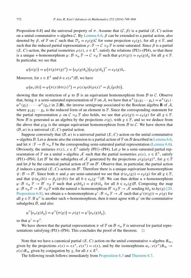
772 P. Ara, R. Exel / Advances in Mathematics 252 (2014) 748–804
Proposition 6.8] and the universal property of π . Assume that (C, β) is a partial (E,C)-actionon a unital commutative ∗-algebra C. By Lemma 6.6, β can be extended to a partial action, alsodenoted by β , of F on C such that Dg = eβ(g)C for some projection eβ(g), for all g ∈ F, andsuch that the induced partial representation ρ :F → C�β F is semi-saturated. Since β is a partial(E,C)-action, the partial isometries ρ(x), x ∈ E1, satisfy the relations (PI1)–(PI4), so that thereis a unique ∗-homomorphism ϕ :B �α F → C �β F such that ϕ(π(g)) = eβ(g)δg for all g ∈ F.In particular, we see that
ϕ(e(g))= ϕ(π(g)π(g)∗
)= (eβ(g)δg
)(eβ(g)δg
)∗ = eβ(g)δe.
Moreover, for x ∈ E1 and b ∈ e(x∗)B, we have
ϕ(αx(b)
)= ϕ(π(x)bπ(x)∗
)= ρ(x)ϕ(b)ρ(x)∗ = βx
(ϕ(b)),
showing that the restriction of ϕ to B is an equivariant homomorphism from B to C. Observethat, being π a semi-saturated representation of F on A, we have that απ(g1g2 · · ·gn) = απ(g1) ·απ(g2) · · · · · απ(gn) in I(B), the inverse semigroup associated to the Boolean algebra B of A,where g1g2 · · ·gn is the reduced form of an element in F. Since the corresponding statement forthe partial representation ρ on C �β F also holds, we see that ϕ(e(g)) = eβ(g) for all g ∈ F.Now B is generated as an algebra by the projections e(g), with g ∈ F, and so we deduce fromthe above that ϕ|B is the unique equivariant homomorphism from B to C. We have shown that(B, α) is a universal (E,C)-partial action.
Suppose conversely that (B, α) is a universal partial (E,C)-action on the unital commutative∗-algebra B. Let α denote also the extension to a partial action of F on B described in Lemma 6.6,and let π :F→ B�α F be the corresponding semi-saturated partial representation (Lemma 6.6).Obviously, the unitaries π(x), x ∈ E1 satisfy (PI1)–(PI4). Let ρ be a semi-saturated partial rep-resentation of F on a unital ∗-algebra A′ such that the partial isometries ρ(x), x ∈ E1, satisfy(PI1)–(PI4). Let B′ be the subalgebra of A′ generated by the projections ρ(g)ρ(g)∗, for g ∈ Fand let β be the canonical partial action of F on B′. Observe that, in particular, the partial actionβ induces a partial (E,C)-action on B′. Therefore there is a unique equivariant homomorphismψ :B → B′. Since both π and ρ are semi-saturated we see that ψ(eα(g)) = eβ(g) for all g ∈ F,and that ψ(αg(b)) = βg(ψ(b)) for all b ∈ eα(g−1)B. We can thus define a ∗-homomorphismϕ :B �α F → B′ �β F such that ϕ(bδg) = ψ(b)δg for all b ∈ eα(g)B. Composing the mapϕ :B�αF→ B′�β F with the natural ∗-homomorphism B′�β F→ A′ sending bδg to bρ(g) [20,Proposition 6.8], we obtain a ∗-homomorphism ϕ′ :B�α F →A′ such that ϕ′(π(g)) = ρ(g) forall g ∈ F. If ϕ′′ is another such ∗-homomorphism, then it must agree with ϕ′ on the commutativesubalgebra B, and also
ϕ′′(eα(g)δg
)= ϕ′′(π(g))= ρ(g) = ϕ′(eα(g)δg
),
so that ϕ′ = ϕ′′.We have shown that the partial representation π of F on B�α F is universal for partial repre-
sentations satisfying (PI1)–(PI4). This concludes the proof of the theorem. �Note that we have a canonical partial (E,C) action on the unital commutative ∗-algebra B∞,
given by the projections e(x) = xx∗, e(x∗) = s(x), and by the isomorphisms αx : e(x∗)B∞ →e(x)B∞ given by conjugation by x, for all x ∈ E1.
The following result follows immediately from Proposition 6.3 and Theorem 6.7.
P. Ara, R. Exel / Advances in Mathematics 252 (2014) 748–804 773
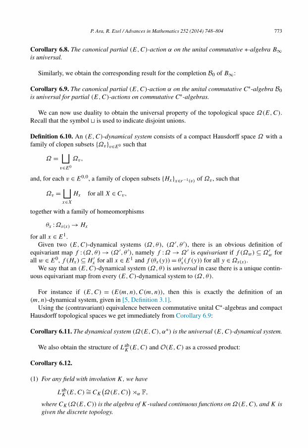
Corollary 6.8. The canonical partial (E,C)-action α on the unital commutative ∗-algebra B∞is universal.
Similarly, we obtain the corresponding result for the completion B0 of B∞:
Corollary 6.9. The canonical partial (E,C)-action α on the unital commutative C∗-algebra B0is universal for partial (E,C)-actions on commutative C∗-algebras.
We can now use duality to obtain the universal property of the topological space Ω(E,C).Recall that the symbol � is used to indicate disjoint unions.
Definition 6.10. An (E,C)-dynamical system consists of a compact Hausdorff space Ω with afamily of clopen subsets {Ωv}v∈E0 such that
Ω =⊔
v∈E0
Ωv,
and, for each v ∈ E0,0, a family of clopen subsets {Hx}x∈r−1(v) of Ωv , such that
Ωv =⊔x∈X
Hx for all X ∈ Cv,
together with a family of homeomorphisms
θx :Ωs(x) → Hx
for all x ∈ E1.Given two (E,C)-dynamical systems (Ω, θ), (Ω ′, θ ′), there is an obvious definition of
equivariant map f : (Ω, θ) → (Ω ′, θ ′), namely f :Ω → Ω ′ is equivariant if f (Ωw) ⊆ Ω ′w for
all w ∈ E0, f (Hx) ⊆ H ′x for all x ∈ E1 and f (θx(y)) = θ ′
x(f (y)) for all y ∈ Ωs(x).We say that an (E,C)-dynamical system (Ω, θ) is universal in case there is a unique contin-
uous equivariant map from every (E,C)-dynamical system to (Ω, θ).
For instance if (E,C) = (E(m,n),C(m,n)), then this is exactly the definition of an(m,n)-dynamical system, given in [5, Definition 3.1].
Using the (contravariant) equivalence between commutative unital C∗-algebras and compactHausdorff topological spaces we get immediately from Corollary 6.9:
Corollary 6.11. The dynamical system (Ω(E,C),α∗) is the universal (E,C)-dynamical system.
We also obtain the structure of LabK (E,C) and O(E,C) as a crossed product:
Corollary 6.12.
(1) For any field with involution K , we have
LabK (E,C) ∼= CK
(Ω(E,C)
)�α F,
where CK(Ω(E,C)) is the algebra of K-valued continuous functions on Ω(E,C), and K isgiven the discrete topology.

774 P. Ara, R. Exel / Advances in Mathematics 252 (2014) 748–804
(2) We have
O(E,C) ∼= C(Ω(E,C)
)�α F,
where C(Ω(E,C)) is the C∗-algebra of continuous functions on Ω(E,C) (here C has theusual topology), and C(Ω(E,C))�α F denotes the full C∗-algebra crossed product.
7. The type semigroup
Let G be a group acting on a set X. Tarski’s Theorem can be expressed as a result on thetype semigroup S(X,G), see [57, Theorem 9.1 and Corollary 9.2]. As Tarski shows in [54, The-orem 16.12], his result holds also if we replace total actions with partial actions. If G acts bycontinuous transformations on a topological space X, and D is a G-invariant subalgebra of sub-sets of X, then we may consider the corresponding type semigroup S(X,G,D) as in [36,37,52].As we will notice in this section, we may as well consider this semigroup for invariant subalge-bras under a partial G-action. An important case, considered in the above references for globalactions, is the case where X is a zero-dimensional metrizable compact space and D is the sub-algebra of P(X) consisting of all the clopen subsets of X. It is an open question in this casewhether the analogue of Tarski’s Theorem holds. The proof of Tarski’s Theorem is based on twospecial properties of the type semigroup S(X,G): the Schröder–Bernstein axiom (also namedCantor–Schröder–Bernstein property) x � y and y � x imply x = y, and the cancellation prop-erty nx = ny ⇒ x = y. The Schröder–Bernstein axiom is known to hold for countably completesubalgebras. However the cancellation law is known to fail even for complete subalgebras [56].
Here we will show that for global actions of free groups on zero-dimensional metrizablecompact spaces, the type semigroup S(X,G,K), where K denotes the subalgebra of all clopensubsets of X, do not satisfy in general any cancellation condition (see Theorem 7.11). In partic-ular we show in Corollary 7.12 the existence, for each pair of positive numbers (m,n) such that1 < m < n, of a global action of a finitely generated free group F on a zero-dimensional metriz-able compact space Ω , such that Ω contains a non-paradoxical but (n,m)-paradoxical clopensubset. This is the first example of the failure of Tarski’s Theorem in this setting.
Our main construction gives in a natural way partial actions on zero-dimensional metrizablecompact spaces. Using globalization results from [1] we get corresponding global actions, al-though on a locally compact, non-compact, Hausdorff space. Passing finally to the one-pointcompactifications of these spaces, we obtain the desired global actions on zero-dimensionalmetrizable compact spaces.
Definition 7.1. Let ({Xt }t∈G, {θt }t∈G) be a partial action of a group G on a set X. Let D be aG-invariant subalgebra of P(X), with Xt ∈D for all t ∈ G. Let S(X,G,D) be the set{
n⋃i=1
Ai × {i}∣∣∣Ai ∈D, n ∈ N
}/ ∼S,
where the equivalence relation ∼S is defined as follows: two sets A =⋃ni=1 Ai × {i} and B =⋃m
j=1 Bj × {j} are equivalent, denoted by A ∼S B , if there exist l ∈ N, Ck ∈ D, tk ∈ G, andnatural numbers nk,mk , k = 1, . . . , l, such that Ck ⊆ X
t−1k
, and
A =l⊔
Ck × {nk}, B =l⊔
θtk (Ck) × {mk}.
k=1 k=1
P. Ara, R. Exel / Advances in Mathematics 252 (2014) 748–804 775
The equivalence class containing A is denoted by [A], and addition is defined by[n⋃
i=1
Ai × {i}]
+[
m⋃j=1
Bj × {j}]
=[
n⋃i=1
Ai × {i} ∪m⋃
j=1
Bj × {n + j}].
Note that S(X,G,D) is a conical refinement monoid, with 0 = [∅]. When D=P(X), S(X,G,D)
is denoted by S(X,G).
A subset E in D is said to be G-paradoxical (with respect to D) in case the element [E] ofS(X,G,D) is properly infinite, that is, 2[E] � [E]. With these definitions we can state Tarski’sTheorem ([57, Corollary 9.2], [54, Theorem 16.12]) as follows:
Theorem 7.2. Let ({Xt }t∈G, {θt }t∈G) be a partial action of a group G on a set X, and let E bea subset of X. Then E is G-non-paradoxical if and only if there exists a monoid homomorphismμ :S(X,G) →R+ ∪ {∞} such that μ([E]) = 1.
The proof of Tarski’s Theorem is based on the following properties of S(X,G) (see [57,Theorem 3.5 and Theorem 8.7]):
(a) Schröder–Bernstein: Let x, y ∈ S(X,G). If x � y and y � x then x = y.(b) n-cancellation: Let n� 1 and x, y ∈ S(X,G). If nx = ny then x = y.
For any semigroup satisfying these two properties, the two conditions stated in Tarski’s Theo-rem are equivalent, that is, if e is a nonzero element in an abelian monoid S satisfying (a) and (b)above, then 2e � e in S if and only if there is a monoid homomorphism μ :S → R+ ∪ {∞} suchthat μ(e) = 1. This is a consequence of a purely semigroup theoretic result [57, Theorem 9.1]. Asobserved in [52, Theorem 5.4], the two conditions stated in Tarski’s Theorem are also equivalentif the abelian semigroup S satisfies the following condition:
(c) almost unperforation: (n + 1)x � ny ⇒ x � y for every n� 1 and x, y ∈ S.
We are interested in the following concrete setting. Let X be a zero-dimensional metrizablecompact Hausdorff space, and let K = K(X) be the subalgebra of P(X) consisting of all theclopen subsets of X. Let ({Xt }t∈G, {θt }t∈G) be a partial action of a group G by continuous trans-formations on X such that Xt ∈ K for all t ∈ G. Observe that K is then automatically G-invariant.Then we want to know to what extent properties (a), (b) or (c) hold in S(X,G,K). In particularwe want to know whether Tarski’s Theorem holds in this context.
We have the following general result in this setting:
Lemma 7.3. Let X be a totally disconnected compact Hausdorff topological space, and let Kbe the subalgebra of P(X) consisting of the clopen subsets of X. Let ({Xt }t∈G, {θt }t∈G) be acontinuous partial action of a group G on X, such that Xt ∈ K for all t ∈ G. Let K be a field,and let CK(X) be the K-algebra of K-valued continuous functions on X, where K is given thediscrete topology. Then there exists a canonical monoid homomorphism
Φ :S(X,G,K) → V(CK(X)�θ∗ G
)sending [⋃n
Ai × {i}] to∑n [1A δe], for Ai ∈K, i = 1, . . . , n.
i=1 i=1 i
776 P. Ara, R. Exel / Advances in Mathematics 252 (2014) 748–804
Proof. Since additivity is clear, we only have to prove that the map is compatible with the equiv-alence ∼S of Definition 7.1. For this it is enough to show that if C ∈ K and C ⊆ Xt−1 for somet ∈ G, then the projections 1Cδe and 1θt (C)δe are equivalent. Set x = 1θt (C)δt , and note thatx∗ = 1Cδt−1 . Then one computes that xx∗ = 1θt (C)δe and x∗x = 1Cδe, showing the result. �
We do not know whether the map defined in the lemma is injective or surjective in general, butwe can show it is bijective for the actions of F on the spaces Ω(E,C) introduced in Section 6.
Theorem 7.4. Let (E,C) be a finite bipartite separated graph such that s(E1) = E0,1 andr(E1) = E0,0, and let (Ω(E,C),α∗) be the universal (E,C)-dynamical system (see Corol-lary 6.11). Then the map
Φ :S(Ω(E,C),F,K
)→ V(CK
(Ω(E,C)
)�α F)
is an isomorphism for any field K .
Proof. By Corollary 6.12(1) and Corollary 5.9, we have
V(CK
(Ω(E,C)
)�α F)∼= V
(Lab(E,C)
)∼= lim−→(M(En,C
n), ιn)∼= M
(F∞,D∞).
Let Φ ′ be the composition of the map Φ with the isomorphism V(CK(Ω(E,C)) �α F) ∼=lim−→(M(En,C
n), ιn). It will suffice to show that Φ ′ is an isomorphism.Observe that there is a basis of clopen subsets of Ω(E,C) which is in bijective correspon-
dence with the vertices in F∞. Indeed, if v ∈ Dn is a vertex in the n-th level, then it representsa minimal projection in the commutative algebra Bn. The image of this projection through thecanonical limit map Bn → B∞ is a projection in B∞, and so corresponds to a clopen subsetof Ω(E,C). Each clopen subset of Ω(E,C) is a finite (disjoint) union of clopen subsets com-ing from the vertices of En for some n. (Note that E0
n = Dn � Dn+1.) The map Φ ′ sends theclass [Av] of the clopen set corresponding to a vertex v ∈ Dn � Dn+1 to the class in the limitlim−→(M(En,C
n), ιn) of the corresponding element av of M(En,Cn).
Put S = S(Ω(E,C),F,K). We are going to build an inverse monoid homomorphismΨ : lim−→(M(En,C
n), ιn) → S. To this end we need to define compatible monoid homomorphisms
Ψn :M(En,Cn) → S. For v ∈ E0
n define Ψn(av) = [Av], where, as before, Av is the clopen sub-set of Ω(E,C) corresponding to v. If X ∈ Cv , with v ∈ E
0,0n , then we have to show that the
relation av =∑z∈X as(z) is preserved by Ψn. Now, it follows from either (5.8) or (5.9) that,for z ∈ X, there is an element uz ∈ E1 ∪ (E1)∗ such that the image of the projection zz∗ inLab(E,C) = A∞ is a projection in B∞ which is of the form αuz(1As(z)
), where the clopen setAs(z) is contained in the domain of α∗
uz. We will show this in the case where n = 2m, and leave
to the reader the verification in the case where n is odd. If n = 0, then z = uz and, using (5.2),the result is clear. Assume that n = 2m > 0. By (5.8) there is uz ∈ E1 and w1, . . . ,wt ∈ Un suchthat z = Φn(uze(w1) · · · e(wt )). As observed at the beginning of the proof of Theorem 5.7, theelements
Φn
(u∗
zuz
),Φn
(e(w1)
), . . . ,Φn
(e(wt )
)are projections in Bn, so that in particular they are mutually commuting projections in An. Thisimplies that
s(z) = z∗z = Φn
(e(u∗)e(w1) · · · e(wt )
),
z
P. Ara, R. Exel / Advances in Mathematics 252 (2014) 748–804 777
and
zz∗ = Φn(uz)(Φn
(e(u∗
z
)e(w1) · · · e(wt )
))Φn(uz)
∗.
Let Φi,∞ :Ai → A∞ be the canonical map into the direct limit. Note that, by (5.2), the ele-ment φn(zz
∗) is a projection in Bn+1, so that Φn,∞(zz∗) = Φn+1,∞(φn(zz∗)) is a projection
in B∞. Now, we have that αuz is given by conjugation by Φ0,∞(uz) = Φn,∞(Φn(uz)) onΦn,∞(Φn(e(u
∗z)))B∞, which shows our claim.
Since v =∑z∈X zz∗ in L(En,Cn), we conclude that
[Av] =∑z∈X
[α∗
uz(As(z))
]=∑z∈X
[As(z)], (7.1)
showing that Ψn preserves the relation av =∑z∈X as(z). To show compatibility with respect to
ιn :M(En,Cn) → M(En+1,C
n+1), observe that, for v ∈ E0,1n , we have
Ψn+1(ιn(av)
)= Ψn+1(av) = [Av] = Ψn(av).
If v ∈ E0,0n then, by the proof of Lemma 4.5(a), (b), we have ιn(av) =∑z∈X as(z), where X is
any element in Cv , so that using (7.1), we get
Ψn+1(ιn(av)
)= Ψn+1
(∑z∈X
as(z)
)=∑z∈X
[As(z)] = [Av] = Ψn(av),
as desired.The homomorphism Ψ : lim−→(M(En,C
n), ιn) → S just defined is clearly a two-sided inverse
of Φ ′. This shows the result. �We can now show our first main result on the type semigroup.
Theorem 7.5. Let M be a finitely generated abelian conical monoid. Then there exist a zero-dimensional metrizable compact Hausdorff space Ω and a partial action of a finitely generatedfree group F on Ω such that there is a map ι :M → S(Ω,F,K) which is a refinement of M . Inparticular, the map ι :M → S(Ω,F,K) is a unitary embedding.
Proof. By Redei’s Theorem [30], M is finitely presented. Let 〈X | R〉 be a finite presentationof M , as in Definition 4.2, and let (E,C) be the associated finite bipartite separated graph, sothat M ∼= M(E,C) (see Definition 4.2).
Let F be the free group on E1, and let (Ω(E,C),α∗) be the universal (E,C)-dynamicalsystem (see Corollary 6.11). By Theorem 7.4, we have that the canonical map
Φ :S(Ω(E,C),F,K
)→ V(CK
(Ω(E,C)
)�α F)
is an isomorphism, and by Corollary 6.12(1) we have
V(CK
(Ω(E,C)
)�α F)∼= V
(Lab(E,C)
).
Since the natural map M(E,C) → V(Lab(E,C)) is a refinement of M(E,C) (Corollary 5.9),and M ∼= M(E,C), we obtain the result. �
In particular, we obtain the following:

778 P. Ara, R. Exel / Advances in Mathematics 252 (2014) 748–804
Corollary 7.6. There exist a partial action of a finitely generated free group F on a zero-dimensional metrizable compact space Ω , and a non-F-paradoxical (with respect to K) clopensubset A of Ω such that μ(A) = ∞ for every nonzero F-invariant finitely additive measureμ :K→ [0,∞].
Proof. Take positive integers m,n such that 1 < m < n, and set (E,C) = (E(m,n),C(m,n)).Set Ω := Ω(E,C). Then there is a canonical partial action of the free group F on m + n
generators on the zero-dimensional metrizable compact space Ω . Moreover, it follows from The-orem 7.5 that there is a unitary embedding
ι : 〈a | ma = na〉 → S(Ω,F,K).
Let A = Aw be the clopen subset corresponding to the vertex w of the graph E (see e.g. Exam-ple 9.3). Then [A] is an order-unit in S(Ω,F,K), and m[A] = n[A]. Since m < n this impliesthat μ(A) = ∞ for every nonzero finitely additive F-invariant measure μ defined on K. Sinceι(a) = [A] and 2a � a in 〈a | ma = na〉, we deduce that 2[A] � [A] in S(Ω,F,K) (use proper-ties (3) and (1) in Definition 3.7). It follows that A is not F-paradoxical (with respect to K). �
We proceed now to extend the above results to the setting of global actions. This is accom-plished by the use of the globalization techniques of [1].
Recall from [1, Example 1.1], that if
β : G × Y → Y
is an action of a given group G on a set Y , and if X ⊆ Y is any subset, one may always restrictβ to X, regardless of whether or not X is β-invariant, obtaining a partial action, as follows: foreach g ∈ G, set Xg = X ∩ βg(X), and observe that
βg(Xg−1) = βg
(X ∩ βg−1(X)
)= βg(X) ∩ X = Xg.
We may then define
αg : Xg−1 → Xg
to be the restriction of βg to Xg−1 , and it may be easily proven that α is a partial action of G
on X, henceforth referred to as the restriction of β to X.Conversely, if we start with a partial action α of G on X, a global (as opposed to partial)
action β on a set Y ⊇ X is called a globalization, or an enveloping action for α [1, Section 1], ifα is the restriction of β to X, and moreover
Y =⋃g∈G
βg(X).
Working in the category of topological spaces, as opposed to the category of sets, we alwaysassume that the transformations αg and βg are continuous and that X is open in Y , in which casewe will clearly have that each Xg is open in X.
It is our next goal to study the relationship between the type semigroup of a partial action α
and that of its globalization or, more generally, any global action extending α.For this let us assume we are given a set Y equipped with a fixed non-empty collection E of
subsets of Y , which is closed under finite intersections, finite unions and relative complements.In other words, E is a ring of subsets of Y . From now on we will refer to the members of E asadmissible subsets.

P. Ara, R. Exel / Advances in Mathematics 252 (2014) 748–804 779
Let us assume that we are also given a fixed admissible subset X ⊆ Y , and let
E|X = {E ∩ X: E ∈ E} = {D ∈ E: D ⊆ X}.It is readily verified that E|X is a subalgebra of subsets of X.
Let us now consider a global action β of a given group G on Y , which we will suppose tobe admissible in the sense that βg(E) is admissible for every admissible subset E ⊆ Y . We maythen consider the corresponding type semigroup S(Y,G,E).
Denoting by α the restriction of β to X, it is clear that each Xg is admissible (relative to E|X)and that α is an admissible partial action in the sense that, if D is an admissible subset of someXg−1 , then αg(D) is admissible.
Given any D ∈ E|X , we shall denote the class of D in S(X,G,E|X) by [D]X . Likewise, theclass in S(Y,G,E) of any E ∈ E will be denoted by [E]Y .
Proposition 7.7. The correspondence
φ : [D]X �→ [D]Y (D ∈ E|X),
gives a well-defined injective map from S(X,G,E|X) to S(Y,G,E).
Proof. We leave the easy verification of the well definedness of φ for the reader. In order to showthat φ is injective, assume that D,D′ ∈ E|X are such that
[D]Y = [D′]Y.
Then there are sets D1, . . . ,Dn ∈ E, such that D =⊔ni=1 Di and, for suitable group elements
g1, . . . , gn, one has that D′ =⊔ni=1 βgi
(Di).Since the Di are subsets of D, and hence also of X, it is evident that Di ∈ E|X . Moreover
notice that
βgi(Di) ⊆ D′ ∩ βgi
(X) ⊆ X ∩ βgi(X) = Xgi
,
so Di ⊆ Xg−1i
, and it thus makes sense to speak of αgi(Di). It is also clear that
D′ =n⊔
i=1
αgi(Di),
so [D]X = [D′]X . The general case, that is, when D and D′ are of the form⋃n
i=1 Di × {i}, maybe treated similarly. �
A case of interest occurs when Y is a Hausdorff topological space and
E = K(Y ) := {E ⊆ Y : E is compact and open}.Given a compact–open subset X ⊆ Y , notice that
K(Y )|X = K(X).
Proposition 7.8. Suppose we are given a continuous global action β of a discrete group G on aHausdorff space Y . Also let X ⊆ Y be a compact–open subset such that
Y =⋃
βg(X).
g∈G
780 P. Ara, R. Exel / Advances in Mathematics 252 (2014) 748–804
Letting α be the restriction of β to X, one has that the map
φ : S(X,G,K(X))→ S
(Y,G,K(Y )
)described above is bijective.
Proof. Given E ∈ K(Y ), we may view {βg(X)}g∈G as an open covering of E. Observing thatE is compact, there are finitely many group elements g1, . . . , gn, such that E ⊆⋃n
i=1 βgi(X).
Setting
E1 = E ∩ βg1(X),
E2 = (E ∩ βg2(X)) \ E1,
E3 = (E ∩ βg3(X)) \ (E1 ∪ E2),
...
En = (E ∩ βgn(X)) \ (E1 ∪ · · · ∪ En−1)
one has that E =⊔ni=1 Ei . Observing that each Ei ⊆ βgi
(X), we have that
Di := βg−1i
(Ei) ⊆ X.
Moreover, φ([Di]X) = [Di]Y = [Ei]Y , so
φ
(n∑
i=1
[Di]X)
=n∑
i=1
φ([Di]X
)= n∑i=1
[Ei]Y = [E]Y .
Since S(Y,G,K(Y )) is generated by the collection of all elements of the form [E]Y , as above,we deduce that φ is surjective. The fact that φ is injective follows from Proposition 7.7. �Corollary 7.9. Let X be a compact Hausdorff topological space which is totally disconnectedin the sense that its topology admits a basis of compact–open sets. Also let α be a continuouspartial action of the group G on X. Then α admits a unique globalization β on a totally dis-connected, locally compact Hausdorff space Y , and moreover S(X,G,K(X)) is isomorphic toS(Y,G,K(Y )).
Proof. By [1, Theorem 1.1] we know that α admits a unique globalization β acting on a topo-logical space Y . Using [1, Proposition 1.2] we may easily show that Y is Hausdorff. Since X isopen in Y , and Y =⋃g∈G βg(X), it is clear that Y is locally compact and totally disconnected.
Finally, observing that X is a compact–open subset of Y , we may use Proposition 7.8 toconclude that S(X,G,K(X)) and S(Y,G,K(Y )) are isomorphic. �
We can now extend Theorem 7.4 to the globalized actions. For a totally disconnected locallycompact Hausdorff space Y and a field K , we denote by Cc,K(Y ) the algebra of continuousfunctions with compact support from Y to K , where K is given the discrete topology. If θ is aglobal action of G on Y we get as in Lemma 7.3 a monoid homomorphism Φ :S(Y,G,K(Y )) →V(Cc,K(Y )�θ∗ G).
Theorem 7.10. Let (E,C) be a finite bipartite separated graph such that s(E1) = E0,1 andr(E1) = E0,0, and let (Ω(E,C),α∗) be the universal (E,C)-dynamical system. Let ΩG(E,C)
P. Ara, R. Exel / Advances in Mathematics 252 (2014) 748–804 781
denote the totally disconnected, locally compact Hausdorff space obtained from the globalizationof the action of F on Ω(E,C) (Corollary 7.9), and let β∗ be the corresponding global action ofF on it.
Then the map
Φ :S(ΩG(E,C),F,K
(ΩG(E,C)
))→ V(Cc,K
(ΩG(E,C)
)�β F)
is an isomorphism for any field K .
Proof. Set X = Ω(E,C) and Y = ΩG(E,C). Let e = 1X ∈ Cc,K(Y ). Then it is easily seen thate is a full projection in Cc,K(Y )�β F such that
e(Cc,K(Y )�β F
)e ∼= CK(X)�α F.
It follows from the first paragraph of the proof of [6, Lemma 7.3] that the map
V(ι) :V(CK(X)�α F
)→ V(Cc,K(Y )�β F
)induced by the inclusion ι :CK(X) �α F → Cc,K(Y ) �β F is an isomorphism. (See also [32,Corollary 5.6] for a more general statement.)
We have a commutative diagram:
S(X,F,K(X))ΦX−−−−→ V(CK(X)�α F)
∼=⏐⏐� V(ι)
⏐⏐�∼=S(Y,F,K(Y ))
ΦY−−−−→ V(Cc,K(Y )�β F)
We observed before that V(ι) is an isomorphism. The map ΦX is an isomorphism by Theo-rem 7.4, and the left vertical map is an isomorphism by Proposition 7.8. Therefore we concludethat ΦY is also an isomorphism. �
We finally can reach our goal of presenting global actions on zero-dimensional metrizablecompact spaces with arbitrary failure of cancellation laws.
Theorem 7.11. Let M be a finitely generated abelian conical monoid. Then there exist a zero-dimensional metrizable compact space Z and a global action of a finitely generated free groupF on Z such that there is an order-embedding ι :M → S(Z,F,K(Z)).
Proof. Let (E,C) be the finite bipartite separated graph considered in the proof of Theo-rem 7.5, and let F be the free group on E1. Let ΩG,�(E,C) = ΩG(E,C) ∪ {�} be the one-pointcompactification of the locally compact Hausdorff space ΩG(E,C), with the action β∗ ex-tended to ΩG,�(E,C) by β∗
t (�) = � for all t ∈ F. Set X = Ω(E,C), Y = ΩG(E,C) andZ = ΩG,�(E,C).
By the proof of Theorem 7.5, there is an order-embedding M ↪→ S(X,F,K(X)), and, byCorollary 7.9, Y is a totally disconnected locally compact Hausdorff space such that the naturalmap
S(X,F,K(X)
)→ S(Y,F,K(Y )
)is an isomorphism. It is easily seen that the natural map S(Y,F,K(Y )) → S(Z,F,K(Z)) isan order-embedding. Combining all these facts we get that Z is a zero-dimensional metrizablecompact space and there is an order-embedding M ↪→ S(Z,F,K(Z)). �
782 P. Ara, R. Exel / Advances in Mathematics 252 (2014) 748–804
Corollary 7.12. There exist a global action of a finitely generated free group F on a zero-dimensional metrizable compact space Z, and a non-F-paradoxical (with respect to K) clopensubset A of Z such that μ(A) = ∞ for every finitely additive F-invariant measure μ :K →[0,∞] such that μ(A) > 0.
Proof. Consider the space X = Ω(E,C) and the clopen subset A appearing in the proof ofCorollary 7.6, and set Z = ΩG,�(E,C) as in the proof of Theorem 7.5. Then A is a clopensubset of Z satisfying the desired conditions. �8. Descriptions of the space Ω(E,C)
We follow with the general hypothesis of Sections 4–6, so that (E,C) is a finite bipartite sep-arated graph with s(E1) = E0,1 and r(E1) = E0,0. In this section we will provide descriptions ofthe zero-dimensional metrizable compact space Ω(E,C) and the partial action of the free groupon E1, F, on the space Ω(E,C). These descriptions generalize the descriptions obtained in [5]for the universal (m,n)-dynamical system.
We will use the notation established in Definition 6.10, so that Ω(E,C) =⊔v∈E0 Ω(E,C)v ,Ω(E,C)v =⊔x∈X Hx for all X ∈ Cv (v ∈ E0,0), and θx :Ω(E,C)s(x) → Hx are the structuralclopen sets and homeomorphisms of the universal (E,C)-dynamical system.
The main point to understand the structure of the space Ω(E,C) is the following: Points inΩ(E,C) are completely determined by their dynamics. Namely, suppose that we have a pointξ in Ω(E,C)w , where w ∈ E0,1. Then we can apply the maps θx to ξ , for all x ∈ E1 suchthat s(x) = w. Given one such arrow x, the point θx(ξ) belongs to Hx ⊆ Ω(E,C)r(x). For eachX ∈ Cr(x) with x /∈ X, we have a decomposition Ω(E,C)r(x) =⊔y∈X Hy , and the point θx(ξ)
belongs to exactly one of these sets Hy , say θx(ξ) ∈ Hy(ξ,x) for a unique y(ξ, x) ∈ X. Then wecan apply the map θ−1
y(ξ,x) to θx(ξ) and obtain a new point in Ω(E,C)s(y(ξ,x)), and again we canrestart the process. The point ξ is determined by the information provided by this infinite process,and conversely any coherent set of data determines a point in the space Ω(E,C).
It is easy to see that Proposition 6.3 generalizes to O(E,C), meaning that the latter is the uni-versal C∗-algebra for semi-saturated partial representations of F satisfying relations (PI1)–(PI4).
We may thus apply [27, Theorem 4.4] to obtain a characterization of Ω(E,C), the spectrumof relations (PI1)–(PI4), as a subset of 2F. The first step is to translate our relations in terms offunctions on 2F. Relative to (PI1) we have the functions:
(F1) f 1x,y(ξ) = [x ∈ ξ ][y ∈ ξ ] − δx,y[x ∈ ξ ], ∀ξ ∈ 2F,
for x, y ∈ X, X ∈ C, where the brackets correspond to boolean value. Speaking of (PI2), we havefunctions of the form:
(F2) f 2x,y(ξ) = [x−1 ∈ ξ
]− [y−1 ∈ ξ],
for all x, y ∈ E1 such that s(x) = s(y). As for (PI3), the functions we consider are:
(F3) f 3X,Y (ξ) =
∑[x ∈ ξ ] −
∑[y ∈ ξ ],
x∈X y∈Y

P. Ara, R. Exel / Advances in Mathematics 252 (2014) 748–804 783
for all X,Y ∈ Cv , v ∈ E0,0. In order to account for (PI4), we must consider a single function,namely:
(F4) f 4(ξ) = −1 +∑
w∈E0,1
[x−1w ∈ ξ
]+ ∑v∈E0,0
∑x∈Xv
[x ∈ ξ ],
where we choose some xw in s−1(w), for each w ∈ E0,1, and some Xv in Cv , for each v ∈ E0,0.Finally, since O(E,C) is the universal C∗-algebra for a collection of partial representations
which are semi-saturated, we must include the functions
f 5g,h(ξ) = [h ∈ ξ ][g ∈ ξ ] − [gh ∈ ξ ],
for all g,h ∈ F, such that |gh| = |g| + |h|. See [22, Proposition 5.4] for more details.Considering the set R formed by all of the above functions, we have by [27, Proposition 4.1],
that
Ω(E,C) = ΩR = {ξ ∈ 2F: 1 ∈ ξ, f(g−1ξ)= 0, for all f ∈R, and all g ∈ ξ
}.
In order to give a more explicit description for this space, let us first introduce some terminol-ogy. Given ξ in 2F, and given g in ξ , we will let ξg be the local configuration of ξ at g, meaningthe set of all elements
x ∈ E1 ∪ (E1)−1
(recall that F is the free group generated by E1), such that gx ∈ ξ . Thus the set gξg consistsprecisely of the elements in ξ whose distance to g equals 1 relative to the Cayley graph metric.
One may then check that Ω(E,C) consists precisely of all ξ ∈ 2F such that:
(a) 1 ∈ ξ ,(b) ξ is convex1 [26, Definition 4.4] and [26, Proposition 4.5],(c) for every g ∈ ξ , there is some v ∈ E0 such that:
(c.1) in the case v ∈ E0,1, the local configuration ξg consists of the elements of the forme−1, for all e ∈ E1 such that s(e) = v (and nothing more),
(c.2) in the case v ∈ E0,0, the local configuration ξg consists of exactly one element of eachgroup X ∈ Cv (and nothing more).
Having completed the description of Ω(E,C), the partial action of F is now easy to describe:for each g ∈ F we put
Ωg = {ξ ∈ Ω(E,C): g ∈ ξ},
and we let
θg : Ωg−1 → Ωg
be given by θg(ξ) = gξ = {gh: h ∈ ξ}.We now start the description of the space Ω(E,C) in terms of certain “choice functions”.To avoid cumbersome considerations, we will from now on assume the following:
1 A subset ξ ⊆ F is said to be convex if, whenever g,h, k ∈ F are such that g,h ∈ ξ and |g−1h| = |g−1k| + |k−1h|,then k ∈ ξ .
784 P. Ara, R. Exel / Advances in Mathematics 252 (2014) 748–804
Hypothesis 8.1. (E,C) is a finite bipartite separated graph such that |Cv| � 2 for all v ∈ E0,0
and s(E1) = E0,1.
This is justified by Proposition 9.2.Given e ∈ E1, there is a unique X ∈ C such that e ∈ X. This unique X will be denoted by Xe.Let v ∈ E0,0. For X ∈ Cv , define
ZX =∏
Y∈Cv,Y =X
Y.
For each Y0 ∈ Cv , Y0 = X, we denote by πY0 the canonical projection map ZX → Y0.We now provide a description of the points belonging to Ω(E,C)w for w ∈ E0,1.
Definition 8.2. A partial E-function for (E,C) is a finite sequence
(Ω1, f1), (Ω2, f2), . . . , (Ωr, fr),
where each Ωi is a certain finite subset of F, and each fi is a function from Ωi to⊔
X∈C ZX
satisfying the following rules:
(1) Ω1 = s−1(w) for some w ∈ E0,1 and f1(e) ∈ ZXe for all e ∈ s−1(w).(2) For each j = 2, . . . , r , Ωj is the set of all the elements of F of the form
e2j−1e−12j−2e2j−3 · · · e−1
4 e3e−12 e1
where
e2j−3 · · · e−14 e3e
−12 e1 ∈ Ωj−1,
e2j−2 = (πY ◦ fj−1)(e2j−3 · · · e−14 e3e
−12 e1) for some Y ∈ C which is a factor of ZX , where
fj−1(e2j−3 · · · e−14 e3e
−12 e1) ∈ ZX , and where e2j−1 ∈ E1 satisfies that s(e2j−1) = s(e2j−2)
and e2j−1 = e2j−2.(3) The function fj :Ωj →⊔X∈C ZX satisfies
fj
(e2j−1e
−12j−2e2j−3 · · · e−1
4 e3e−12 e1) ∈ ZXe2j−1
for all e2j−1e−12j−2e2j−3 · · · e−1
4 e3e−12 e1 ∈ Ωj . Note that, by Hypothesis 8.1, there is always
at least one such function fj .
An E-function is an infinite sequence (Ω1, f1), (Ω2, f2), . . . satisfying the above conditions forall j = 1,2,3, . . . .
Note that it might happen that for some E-function (Ω1, f1), (Ω2, f2), . . . we have Ωr = ∅for some r � 2. In this case the E-function will be of the form
(Ω1, f1), (Ω2, f2), . . . , (Ωr−1, fr−1), (∅,∅), (∅,∅), . . . .
This case occurs for instance for the separated graph (E,C) with E0,0 = {v}, E0,1 = {w1,w2},and C = Cv = {X,Y } with X = {α}, Y = {β}, s(α) = s(β) = v and r(α) = w1, r(β) = w2.
Note that every partial E-function (Ω1, f1), . . . , (Ωr, fr) can be extended to an E-function(Ω1, f1), . . . , (Ωr, fr), (Ωr+1, fr+1), . . . , although possibly Ωi = ∅ for all sufficiently large i.
P. Ara, R. Exel / Advances in Mathematics 252 (2014) 748–804 785
Another degenerate case is the case where there is only one extension of (Ω1, f1), . . . , (Ωr, fr)
to an E-function (Ω1, f1), . . . , (Ωr, fr), (Ωr+1, fr+1), . . . , but Ωi = ∅ for all i. Note thatthis happens for instance for the unique partial E-function (Ω1, f1) of the separated graph(E(1,1),C(1,1)).
Theorem 8.3. Let Ω(E,C) be the universal space associated to the separated graph (E,C),and let w be a vertex in E0,1. Then the points of Ω(E,C)w are in one-to-one correspondencewith the E-functions (Ω1, f1), (Ω2, f2), . . . such that Ω1 = s−1(w). Moreover, given a pointξ in Ω(E,C)w , represented by the E-function (Ω1, f1), (Ω2, f2), . . . , the partial E-functions(Ω1, f1), (Ω2, f2), . . . , (Ωr, fr), r � 1, represent a fundamental system of clopen subsets of ξ inΩ(E,C). The clopen set represented by the partial E-function (Ω1, f1), (Ω2, f2), . . . , (Ωr, fr)
corresponds to a vertex in F∞ lying in the 2r + 1 level D2r+1 of F 0∞ =⊔∞i=0 Di .
Proof. One can show, using arguments similar to those in [5, proof of Theorem 4.1] that theset of E-functions (Ω1, f1), (Ω2, f2), . . . , such that Ω1 = s−1(w) for w ∈ E0,1, is in bijectivecorrespondence with the set of configurations ξ ∈ ΩR such that the local configuration ξ1 of ξ
at 1 consists of elements of the form e−1 for all e ∈ s−1(w) (form (c.1)).We now proceed to show the statement about the relation between partial E-functions and
vertices in the graph F∞. First, we show that the partial E-functions (Ω1, f1) such that Ω1 =s−1(w) (for w ∈ D1), correspond to vertices v in D3 such that r3(v) = w, where rn :Dn → Dn−2is the map defined just before Lemma 5.2. Suppose that Ω1 = s−1(w) = {x1, . . . , xr}. For i =1, . . . , r , consider
yi := αxi(f1(xi)
) ∈ E11 . (8.1)
This has sense because f1(xi) ∈∏Y∈Cr(xi ),Y =Xxi
Y . Note that there are exactly r distinct ele-
ments in Cw , namely X(x1), . . . ,X(xr), and that yi ∈ X(xi) for all i. We can therefore build theelements
zi = αyi (y1, . . . , yi , . . . , yr ) ∈ E12
for i = 1, . . . , r , and the vertex v := v(y1, . . . , yr ) ∈ D3. Note that s−1(v) = {z1, . . . , zr}, so thereis a canonical bijection xi ↔ zi between s−1(w) and s−1(v). The vertex v just constructed is thevertex associated to the partial E-function (Ω1, f1). Conversely, the vertex v = v(y1, . . . , yr )
determines y1, . . . , yr , which in turn determine the function f1 by using (8.1).We will show that a partial E-function
(Ω1, f1), . . . , (Ωr, fr),
with r � 1, for (E,C), such that Ω1 = s−1(w), corresponds to a partial E-function(Ω ′
1, f′1
), . . . ,(Ω ′
r−1, f′r−1
)for the separated graph (E2,C
2), such that Ω ′1 = s−1(v), where v is the vertex in D3 = E
0,12
corresponding to (Ω1, f1) (under the correspondence defined above). By induction hypothesis,this determines (and is determined by) a vertex v′ in (F ′∞)0,2r−1, where F ′∞ is the F -graphassociated to (E2,C
2) (see Construction 4.4). Since F ′∞ is the separated graph obtained fromF∞ by eliminating its two first levels, we see that the original partial E-function corresponds tothe vertex v′ in F
0,2r+1∞ = D2r+1.

786 P. Ara, R. Exel / Advances in Mathematics 252 (2014) 748–804
So we only need to prove the desired correspondence between partial E-functions for (E,C)
and (E2,C2). Observe that, given a vertex v′ in D3 such that r3(v
′) = v ∈ D1, there is a canonicalbijective map between s−1(v) and s−1(v′). We will denote this bijection by e ↔ e′, for e ∈s−1(v). Now take e in s−1(v). Then the corresponding arrow e′ has an end vertex r(e′) and weare going to check that r2(r(e
′)) = r(e).We have s(e′) = v(y1, . . . , yl) and e′ = αyt (y1, . . . , yt , . . . , yl) for some t , where s−1(s(e)) =
{x1, . . . , xl} and xt = e. Now set
Cr(xt ) = Cr(e) = {X1, . . . ,Xs}and write xt = xp ∈ Xp for a unique p ∈ {1, . . . , s}. Then there are xi ∈ Xi for i = p such that
yt = αxp (x1, . . . , xp, . . . , xs).
Note that e ∈ Xp , so that Xe = Xp . On the other hand
r(e′)= r
(αyt (y1, . . . , yt , . . . , yl)
)= s(yt ) = v(x1, . . . , xs),
so that r2(r(e′)) = r(e). It follows that there is a canonical bijective correspondence between
Cr(e) and Cr(e′) (see Lemma 5.2 and Remark 5.3), and we will denote this correspondence byX ↔ X′ for X ∈ Cr(e). Note that Xe′ = X′
e.Let (Ω1, f1), . . . , (Ωr, fr) be a partial E-function for (E,C), where r > 1. Let w ∈ E0,1
be such that Ω1 = s−1(w), and let w′ be the vertex in D3 corresponding to (Ω1, f1). We firstdefine (Ω ′
1, f′1). Let Ω ′
1 = {e′ | e ∈ Ω1}. Then f ′1 is determined as follows. Given e′ ∈ Ω ′
1, thereis a unique e ∈ Ω1 = s−1(w) corresponding to it through the bijection between s−1(w′) ands−1(w). Now we are going to define f ′
1(e′) ∈ ZXe′ . Adopt the notation of the above paragraph,
so that e′ = αyt (y1, . . . , yt , . . . , yl) for some t , where s−1(s(e)) = {x1, . . . , xl} and xt = e. Nowset Cr(xt ) = Cr(e) = {X1, . . . ,Xs} and write e = xp ∈ Xp for a unique p ∈ {1, . . . , s}. Then thereare xi ∈ Xi for i = p such that
yt = αxp (x1, . . . , xp, . . . , xs).
For i = p, we have X′i ∈ Cr(e′), and X′
i = X′p = X′
e = Xe′ , and we aim to define πX′i(f ′
1(e′)).
First set
yi = αxi (x1, . . . , xi, . . . , xs).
Observe that r(yi) = s(xi). Moreover, note that it follows from (8.1) that xi = πXi(f1(e)). The
elements in Cr(yi ) are in bijective correspondence with the elements in s−1(s(xi)). Write S =s−1(s(xi)) \ {xi}. Observe that, since xi = πXi
(f1(e)), the element xx−1i e belongs to Ω2 for
all x ∈ S . Define πX′i(f ′
1(e′)) = αyi ((yi,x)x∈S), where
yi,x = αx(f2(xx−1
i e))
.
Note that, for Xi as above, with i = p, we have
r3(s(πX′
i
(f ′
1
(e′))))= s(xi) = s
(πXi
(f1(e)))
,
so that given any element e′3(πX′
i(f ′
1(e′)))−1e′ in Ω ′
2 we can form a corresponding element
e3(πXi(f1(e)))
−1e in Ω2.Assume that for some r > j > 1, we have defined a partial E-function (Ω ′
1, f′1), . . . ,
(Ω ′ , f ′ ) on (E2,C2) satisfying the following conditions:
j−1 j−1
P. Ara, R. Exel / Advances in Mathematics 252 (2014) 748–804 787
(1) For all 1 � j0 < j and all e′2j0+1(e
′2j0
)−1 · · · e′3(e
′2)
−1e′1 in Ω ′
j0+1 we have r3(s(e′2j0
)) =s(e2j0), where e2j0 is inductively defined by e2j0 = πY (fj0(e2j0−1e
−12j0−2 · · · e3e
−12 e1)) if
e′2j0
= πY ′(f ′j0
(e′2j0−1(e
′2j0−2)
−1 · · · e′3(e
′2)
−1e′1)) for some Y ∈ Cr(e2j0−1) \ {Xe2j0−1}.
Therefore we have a well-defined element e2j0+1(e2j0)−1 · · · e3e
−12 e1 in Ωj0+1 for each ele-
ment e′2j0+1(e
′2j0
)−1 · · · e′3(e
′2)
−1e′1 in Ω ′
j0+1.
(2) For all 1 � j0 < j , all e′2j0−1(e
′2j0−2)
−1 · · · e′3(e
′2)
−1e′1 ∈ Ω ′
j0, all X ∈ Cr(e2j0−1) \ {Xe2j0−1},
and all x ∈ s−1(s(πXfj0(e2j0−1e−12j0−2 · · · e3e
−12 e1))) \ {πXfj0(e2j0−1e
−12j0−2 · · · e3e
−12 e1)},
we have
πx
(πX′f ′
j0
(e′
2j0−1
(e′
2j0−2
)−1 · · · e′3
(e′
2
)−1e′
1
))= αx(fj0+1
(x(πXfj0
(e2j0−1 · · · e−1
2 e1))−1
e2j0−1 · · · e3e−12 e1))
,
where πx denotes the projection πX(x), being X(x) the element in Cs(x) corresponding to x.
Note that indeed condition (2) implies condition (1), but we found useful to state condition (1).As we have seen before, both conditions hold when j0 = 1.
To complete the induction step, we have to define the map f ′j . This is done essentially as in
the case j = 1, only the notation is a little bit worse.Let e′
2j−1(e′2j−2)
−1 · · · (e′2)
−1e′1 be an element in Ω ′
j , and let e2j−1e−12j−2 · · · e−1
2 e1 be the
corresponding element in Ωj (see condition (1)). We want to define f ′j (e
′2j−1(e
′2j−2)
−1 · · ·(e′
2)−1e′
1) ∈ ZX′e2j−1
.
We have s(e′2j−1) = v(y1, . . . , yl) and e′
2j−1 = αyt (y1, . . . , yt , . . . , yl) for some t , where
s−1(s(e2j−1)) = {x1, . . . , xl} and xt = e2j−1. Now set
Cr(xt ) = Cr(e2j−1) = {X1, . . . ,Xk}and write xt = xp ∈ Xp for a unique p ∈ {1, . . . , k}. Then there are xi ∈ Xi for i = p such that
yt = αxp (x1, . . . , xp, . . . , xk).
We have to check that xi = πXi(fj (e2j−1 · · · e−1
2 e1)) for i = p. For this we need condition (2).Indeed, observe that there is s = t such that
e′2j−2 = αys (y1, . . . , ys , . . . , yl).
Observe that
e′2j−2 = πXe′2j−2
(f ′
j−1
(e′
2j−3 · · · (e′2
)−1e′
1
)).
On the other hand
πxt
(e′
2j−2
)= πxt
(αys (y1, . . . , ys , . . . , yl)
)= yt ,
so that, putting everything together and using (2), we get
yt = πxt πXe′2j−2
(f ′
j−1
(e′
2j−3 · · · (e′2
)−1e′
1
))= αxt
(fj
(e2j−1e
−1 e2j−3 · · · e−1e1))
2j−2 2

788 P. Ara, R. Exel / Advances in Mathematics 252 (2014) 748–804
because e2j−2 = πXe2j−2(fj−1(e2j−3 · · · e−1
2 e1)) and e2j−1 = xt . This shows that, for i = p, we
have xi = πXi(fj (e2j−1 · · · e−1
2 e1)), as desired.For i = p, we have X′
i ∈ Cr(e′2j−1)
, and X′i = X′
p = Xe′2j−1
, and we aim to define
πX′i(f ′
j (e′2j−1 · · · (e′
2)−1e′
1)). First set
yi = αxi (x1, . . . , xi, . . . , xk).
Observe that r(yi) = s(xi).The elements in Cr(yi ) are in bijective correspondence with the elements in s−1(s(xi)).
Write S = s−1(s(xi)) \ {xi}. Observe that, since xi = πXi(fj (e2j−1 · · · e−1
2 e1)), the elementxx−1
i e2j−1 · · · e−12 e1 belongs to Ωj+1 for all x ∈ S . Define
πX′i
(f ′
j
(e′
2j−1 · · · (e′2
)−1e′
1
))= αyi((yi,x)x∈S
),
where
yi,x = αx(fj+1(xx−1
i e2j−1 · · · e−12 e1))
.
Note that, for Xi as above, with i = p, we have
r3(s(πX′
i
(f ′
j
(e′
2j−1 · · · (e′2
)−1e′
1
))))= s(xi) = s(πXi
(fj
(e2j−1 · · · e−1
2 e1)))
,
so that given any element e′2j+1(e
′2j )
−1 · · · (e′2)
−1e′1 in Ω ′
j+1 we can form a corresponding el-
ement e2j+1e−12j · · · e−1
2 e1 in Ωj+1. This shows (1) for j , while (2) for j follows from theconstruction.
It follows from (2) that the partial E-function (Ω1, f1), . . . , (Ωr, fr) is completely determinedby (Ω ′
1, f′1), . . . , (Ω
′r−1, f
′r−1). (Notice that knowledge of the latter provides knowledge of the
initial vertex w′ in D3 = E0,12 .)
Now observe that the points in F∞ are in bijective correspondence with a basis of clopensubsets for the topology of Ω(E,C). Given an E-function (Ω1, f1), (Ω2, f2), . . . we have adescending chain of clopen subsets U1 ⊇ U2 ⊇ · · · , where Ur is the clopen set corresponding to(Ω1, f1), . . . , (Ωr, fr). The intersection
⋂∞i=1 Ui will be non-empty, and using that Ω(E,C) is
Hausdorff, it is easy to check that it consists of a single point ξ in Ω(E,C). This completes theproof of the theorem. �Remarks 8.4. (1) In certain applications of [26, Theorem 4.4], notably to the case of the freegroup, the elements ξ in the space ΩR may be more or less completely described by meansof their intersections with the positive cone in the free group. Moreover, this intersection oftenconsists of the prefixes of a certain infinite word (in the positive generators), called the “stem”of ξ , which therefore completely determines the configuration ξ . However, due to the zig-zagnature of the configurations present in Ω(E,C), no such easy description is available. Our useof partial E-functions is therefore an attempt at giving a concrete description of these highlyintricated configurations.
(2) We now give the intuitive idea behind the concept of an E-function. Let ξ ∈ Ω(E,C)w ,where w ∈ E0,1. Consider the picture of ξ as a subset of vertices in the Cayley graph Γ of the freegroup F generated by E1. The intersection ξ ∩ B1 of ξ with the ball of radius 1 (centered at 1)does not involve any choice, since it is given by 1 and all vertices e−1, where e ∈ s−1(w) (becausethe local configuration ξ1 of ξ at 1 is of type (c.1)). The intersection ξ ∩B2 with the ball of radius

P. Ara, R. Exel / Advances in Mathematics 252 (2014) 748–804 789
2 involves the choices which are codified by the function f1 : s−1(w) →⊔X∈C ZX , because, fore ∈ s−1(w), the local configuration ξe−1 of ξ at e−1 must be of type (c.2). In particular the verticesat distance 2 from the origin are the elements of the form e−1πX(f1(e)), for all e ∈ s−1(w) andall X ∈ Cr(e) with X = Xe. In general, the vertices which are at distance 2r − 1 of the originare completely determined by the vertices which are at distance 2r − 2, and the choice functionfr determines the vertices which are at distance 2r from the vertices at distance 2r − 1. Inconclusion knowing the partial E-function (Ω1, f1), . . . , (Ωr, fr) of ξ is equivalent to knowingthe intersection of ξ with the ball B2r . Of course, this can be identified with the set of paths inthe Cayley graph connecting 1 to a vertex in ξ at distance 2r from 1. Obviously, the element ξ isdetermined by the intersections ξ ∩ B2r for all r � 1.
(3) The hardest part of the proof of Theorem 8.3 consists in showing the deep fact that knowl-edge of the intersection ξ ∩ B2r is equivalent to knowledge of a vertex in the 2r + 1 layer D2r+1of the graph F∞ associated to (E,C) in Construction 4.4. �
The action of F on (partial) E-functions is described in our next result.
Lemma 8.5. Let
g = z−1r xrz
−1r−1xr−1 · · · z−1
1 x1
be a reduced word in F, where x1, . . . , xr , z1, . . . , zr ∈ E1. Then Dom(θg) = ∅ unless zi ∈ Yi forsome Yi ∈ Cr(xi) with Yi = Xxi
for all i = 1, . . . , r , and s(xi+1) = s(zi) for i = 1, . . . , r − 1. As-sume that the latter conditions hold. Then the domain of θg is precisely the set of all E-functionsf= ((Ω1, f1), (Ω2, f2), . . .) such that Ω1 = s−1(s(x1)) and
πYifi
(xi · · · z−1
2 x2z−11 x1)= zi
for all i = 1, . . . , r , and the range of θg is the set of those E-functions f′ = (f ′1, f
′2, . . . , ) such
that πXxr−i+1f ′
i (zr−i+1 · · · zr−1x−1r zr ) = xr−i+1 for all i = 1, . . . , r . Moreover for f ∈ Dom(θg)
let f′ = gf denote the image of f under the action of g. Then f′ = ((Ω ′1, f
′1), (Ω
′2, f
′2), . . .) with
f ′r+t
(y2t−1 · · ·y−1
2 y1x−11 z1 · · · zr−1x
−1r zr
)= ft
(y2t−1 · · ·y−1
2 y1)
if y2t−1 · · ·y−12 y1 ∈ Ωt and y1 = x1.
Moreover, for i = 2,3, . . . , r and y2t−1 · · ·y−12 y1z
−1i−1xi−1 · · · z−1
1 x1 ∈ Ωt+i−1 with y1 = xi ,
f ′r−i+1+t
(y2t−1 · · ·y−1
2 y1x−1i zi · · · zr−1x
−1r zr
)= fi−1+t
(y2t−1 · · ·y−1
2 y1z−1i−1xi−1 · · · z−1
1 x1),
and for y2t−1 · · ·y−12 y1z
−1r xr · · · z−1
2 x2z−11 x1 ∈ Ωt+r we have
f ′t
(y2t−1 · · ·y−1
2 y1)= fr+t
(y2t−1 · · ·y−1
2 y1z−1r xr · · · z−1
2 x2z−11 x1).
Proof. The result is clear once we realize that the action of g on a point ξ in Ω(E,C)s(x1)
consists in moving ξ using the composition θ−1zr
θxr · · · θ−1z1
θx1 , in case this is possible. �Notice that, for g as in Lemma 8.5, the condition that Dom(θg) = ∅ is precisely the condition
that the path z∗r xr · · · z∗
1x1 is an admissible path in the double E of E (see Section 10 below forthe definition of admissible path). For such an element g ∈ F and ξ ∈ Dom(θg), we have that theconfiguration θg(ξ) is just a translation of the configuration ξ .

790 P. Ara, R. Exel / Advances in Mathematics 252 (2014) 748–804
9. Examples
Our first example is of a generic type. At first sight, it looks restrictive to concentrate at-tention to bipartite separated graphs. However, the following result shows that (modulo Moritaequivalence) all graph C∗-algebras (or Leavitt path algebras) can be studied that way. For ageneral separated graph (E,C) we define Lab(E,C) (respectively O(E,C)) as the quotient ofL(E,C) (respectively C∗(E,C)) by the ideal (resp. closed ideal) generated by the commutators[e(u), e(u′)], for all u,u′ ∈ U , where U is the multiplicative semigroup generated by E1 � (E1)∗,and e(u) = uu∗.
Proposition 9.1. Let (E,C) be a separated graph. Then there exists a bipartite separated graph(E, C) such that
LK(E, C) ∼= M2(LK(E,C)
), C∗(E, C) ∼= M2
(C∗(E,C)
).
Moreover we have
LabK (E, C) ∼= M2
(Lab
K (E,C)), O(E, C) ∼= M2
(O(E,C)
).
Proof. Let V0 and V1 be two disjoint copies of E0, and denote the canonical maps E0 → Vi byv �→ vi for i = 0,1. Write E0,0 = V0 and E0,1 = V1. Now E1 will be the disjoint union of a copyof E0 and a copy of E1:
E1 = {hv
∣∣ v ∈ E0} � {e0∣∣ e ∈ E1},
with
r(hv) = v0, s(hv) = v1, r(e0) = r(e)0, s(e0) = s(e)1(v ∈ E0, e ∈ E1).
Denote by eij , 0 � i, j � 1 the standard matrix units of M2(K). We define maps ϕ :L(E, C) →M2(L(E,C)) and ψ :M2(L(E,C)) → L(E, C) by the rules
ϕ(vi) = v ⊗ eii , ϕ(hv) = v ⊗ e01, ϕ(e0) = e ⊗ e01(v ∈ E0, e ∈ E1, i = 0,1
),
and
ψ(v ⊗ eii) = vi, ψ(v ⊗ e01) = hv
(v ∈ E0, i = 0,1
),
ψ(e ⊗ e00) = e0h∗s(e), ψ(e ⊗ e11) = h∗
r(e)e0,
ψ(e ⊗ e01) = e0, ψ(e ⊗ e10) = h∗r(e)e0h
∗s(e)
(e ∈ E1).
It is straightforward (though somewhat tedious) to check that ϕ and ψ give well-defined∗-homomorphisms which are mutually inverse. Let U and U denote the multiplicative semi-groups of the algebras L(E,C) and L(E, C) generated by E1 � (E1)∗ and E1 � (E1)∗ respec-tively. Let J denote the ideal of L(E,C) generated by all elements of the form [e(u), e(u′)],with u,u′ ∈ U , and let J denote the corresponding ideal of L(E, C). Then it is easy to checkthat, for u ∈ U , ϕ(e(u)) is a matrix consisting of an element of the form e(u), for some u ∈ U ,in one of the two main diagonal positions and 0s in the rest of positions. This clearly impliesthat ϕ(J ) ⊆ M2(J ). Since the image by ψ of an element of the form u ⊗ e00, for u ∈ U , belongsclearly to U , we see that the reverse containment M2(J ) ⊆ ϕ(J ) also holds. Thus ϕ(J ) = M2(J )
and we conclude that ϕ defines an isomorphism from Lab(E, C) onto M2(Lab(E,C)), as desired.

P. Ara, R. Exel / Advances in Mathematics 252 (2014) 748–804 791
The same proof applies (thanks to the universal properties of the involved C∗-algebras) toshow the corresponding result for the graph C∗-algebras. �
In particular, since any classical graph C∗-algebra C∗(E) satisfies that the final projections[e(u), e(u′)] = 0 for all u,u′ ∈ U , we see that O(E) = C∗(E) can always be interpreted (througha very concrete Morita equivalence) as a graph C∗-algebra of a bipartite separated graph. A sim-ilar statement applies to Leavitt path algebras. The description of a Leavitt path algebra in termsof a crossed product by a partial action has been recently achieved by Gonçalves and Royerin [31].
We are now going to show that we can always reduce our study of the graph algebras of finitebipartite separated graphs, up to Morita equivalence and finite-dimensional summands, to thestudy of finite bipartite separated graphs satisfying Hypothesis 8.1.
Proposition 9.2. Let (E,C) be a finite bipartite separated graph. Then there exists a finite bipar-tite separated graph (E′,C′) satisfying Hypothesis 8.1 such that LK(E,C) is Morita equivalentto LK(E′,C′) ⊕ Kn for some n � 0. Similar statements hold for C∗(E,C), Lab(E,C) andO(E,C).
Proof. Suppose that there is v ∈ E0,0 such that |Cv| = 1. Let (F,D) be the bipartite separatedgraph such that F 0,0 = E0,0 \ {v}, F 0,1 = E0,1, and F 1 = E1 \ r−1(v). Set p =∑w∈E0\{v} w.Then p is a full projection in LK(E,C) such that
LK(F,D) ∼= pLK(E,C)p.
Therefore LK(E,C) is Morita equivalent to LK(F,D). We can apply this process to suppressall the vertices v′ in E0,0 such that |Cv′ | = 1, and thus we arrive at a bipartite separated graph(E, C) such that LK(E,C) is Morita equivalent to LK(E, C) and |Cw| = 1 for all w ∈ E0,0.
Now let (E′,C′) be the bipartite separated graph obtained from (E, C) by deleting all thevertices in E0,0 \ r(E1) and all the vertices in E0,1 \ s(E1). Then clearly (E′,C′) satisfies Hy-pothesis 8.1, and LK(E, C) ∼= LK(E′,C′) ⊕ Kn, where n = |E0| − |r(E1)| − |s(E1)|. Thisshows the result. �
We start our description of concrete examples with a motivational example for the entiretheory of separated graphs, see [8,7,4,5].
Example 9.3.For integers 1 � m� n, define the separated graph (E(m,n),C(m,n)), where
(1) E(m,n)0 := {v,w} (with v = w).(2) E(m,n)1 := {α1, . . . , αn,β1, . . . , βm} (with n + m distinct edges).(3) s(αi) = s(βj ) = v and r(αi) = r(βj ) = w for all i, j .(4) C(m,n) = C(m,n)v := {X,Y }, where X := {α1, . . . , αn} and Y := {β1, . . . , βm}.
See Fig. 1 for a picture in the case m = 2, n = 3. By [8, Proposition 2.12],
L(E(m,n),C(m,n)
)∼= Mn+1(L(m,n)
)∼= Mm+1(L(m,n)
),
where L(m,n) is the classical Leavitt algebra of type (m,n). The same argument (by way ofuniversal properties) shows that

792 P. Ara, R. Exel / Advances in Mathematics 252 (2014) 748–804
Fig. 1. The separated graph (E(2,3),C(2,3)).
Fig. 2. The separated graph of pure refinement.
C∗(E(m,n),C(m,n))∼= Mn+1
(Unc
m,n
)∼= Mm+1(Unc
m,n
),
where Uncm,n denotes the C∗-algebra generated by the entries of a universal unitary m × n matrix,
as studied by Brown and McClanahan in [17,42–44].The C∗-algebras Om,n and Or
m,n studied in [5] are precisely the C∗-algebras O(E(m,n),
C(m,n)) and Or (E(m,n),C(m,n)) in the notation of the present paper. (See Definition 10.7for the definition of the reduced C∗-algebra Or (E,C).) It was shown in [5] that these twoC∗-algebras are not isomorphic.
The algebras Labm,n(K) := Lab
K (E(m,n),C(m,n)) have not appeared before in the literature.They provide natural examples (indeed universal examples) of actions on a compact Hausdorffspace supporting (m,n)-paradoxical decompositions (Corollary 7.6).
We now proceed to describe several concrete examples of separated graphs and their asso-ciated algebras. Curiously enough, these algebras (or the dynamical systems underlying them)have appeared before in the literature in different contexts. In many cases, one has to look at anappropriate full corner of the algebras to find the significant construction.
Example 9.4. Our first example is the “pure refinement” example, given in Fig. 2. Let (E,C) bethe separated graph described by that picture, with Cv = {X,Y } and X = {α1, α2}, Y = {β1, β2}.The corner vLK(E,C)v is isomorphic to a free product K2 ∗K K2. The corner of the abelianizedLeavitt algebra Lab
K (E,C) is isomorphic to K4. We thus see a drastic reduction of the complex-ity in the transition from L(E,C) to Lab(E,C). A similar statement holds for the C∗-algebrasC∗(E,C) and O(E,C).
Example 9.5. Let (E,C) be the separated graph described in Fig. 3, with Cv = {X,Y } andX = {α0, α1} and Y = {β0, β1}.
The Leavitt path algebra LK(E,C) is Morita equivalent to the corner vL(E,C)v, which isisomorphic to M2(K) ∗K M2(K).

P. Ara, R. Exel / Advances in Mathematics 252 (2014) 748–804 793
Fig. 3. The separated graph corresponding to Truss example.
By Corollary 6.12, LabK (E,C) ∼= CK(Ω(E,C))�F4, where Ω := Ω(E,C) is a 0-dimensional
compact space admitting a decomposition Ω = X � Y � Z into clopen subsets, such that Z de-composes in two different ways as a disjoint union of clopen subsets Z = H0 � H1 = V0 � V1,together with homeomorphisms hi :X → Hi for i = 0,1, and vj :Y → Vj for j = 0,1. Thisconstruction is closely related to Truss example in [56], which we briefly describe now. Let E bethe non-directed graph with vertices {vi | i ∈ Z} and with an edge connecting a vertex vi withvi+1, for all i ∈ Z. Let T be the set of all the “labelings” of the edges and vertices of E satisfyingthe following conditions:
(i) the vertices are labeled 0 or 1, and adjacent vertices have different labels,(ii) the edges are labeled by pairs (i, j) where i, j ∈ {0,1},
(iii) if (i, j), (k, l) are the labels on the edges incident with a vertex labeled 0 then i = k.(iv) if (i, j), (k, l) are the labels on the edges incident with a vertex labeled 1 then j = l.
Let
X = {t ∈ T∣∣ v0 is labeled 0 and (v0, v1) is labeled (0,∗)
},
Y = {t ∈ T∣∣ v0 is labeled 1 and (v0, v1) is labeled (∗,1)
}.
Observe that (v−1, v0) is labeled (1,∗) (respectively (∗,0)) for every t in X (respectively Y ).Let T ′ be a disjoint copy of T , with vertices v′
i and with the same conditions on the labels ofvertices and edges. Let ι :T → T ′ be the canonical map. Set
Z = {t ′ ∈ T ′ ∣∣ v′0 is labeled 0
}.
Consider the shift map S :T → T defined by the following conditions: S(t) is the labeledgraph such that the label of S(t) at vi is the label of t at vi−1, and the label of S(t) at (vi, vi+1) isthe same as the label of t at (vi−1, vi). Let S′ = ι ◦ S ◦ ι−1 be the corresponding bijection of T ′.
We also need the involution φ :T → T , which sends any t ∈ T to the labeled graph φ(t)
defined by the condition that the bijection vi → v−i on the set of vertices {vi | i ∈ Z} is anisomorphism of labeled graphs between t and φ(t).
We first indicate the connection between the definition using E-functions (see Theo-rem 8.3) and the description above. Consider an E-function (Ω1, f1), (Ω2, f2), . . . , whereΩ1 = s−1(w0) = {α0, α1}. This E-function will correspond, upon identification of the la-bels (i, j) with the labels (αi, βj ), to an element t of X, as follows. The function f1 takesvalues on {β0, β1} so we define the label at the edge (v0, v1) as (α0, f1(α0)) and the la-bel at the edge (v−1, v0) as (α1, f1(α1)). Now the label at the edge (v1, v2) is defined by(f2(f1(α0)f1(α0)
−1α0), f1(α0)), where we set αi = α1−i and βj = β1−j . Similarly, the labelat the edge (v−2, v−1) is defined by (f2(f1(α1)f1(α1)
−1α1), f1(α1)). Continuing in this way,we define the labels at all the edges (vi, vi+1). The labels at vertices are defined so as to maket an element of X. It is easy to see that this procedure establishes a bijection between the set of

794 P. Ara, R. Exel / Advances in Mathematics 252 (2014) 748–804
Fig. 4. The separated graph of a partial isometry.
E-functions (Ω1, f1), (Ω2, f2), . . . with Ω1 = s−1(w0) and X. Similarly there is a bijection be-tween the set of E-functions (Ω1, f1), (Ω2, f2), . . . with Ω1 = s−1(w1) and Y . For each r � 1,the intersection of an element ξ ∈ X with the ball B2r in the Cayley graph of F4 has exactly twovertices: the one obtained by going in the “positive direction”, and the one obtained by going inthe “negative direction”.
We are now in a position to describe the maps hi ,vj in our picture of Ω . Set
H0 = {t ′ ∈ Z∣∣ (v′
0, v′1
)is labeled (0,∗)
}, H1 = {t ′ ∈ Z
∣∣ (v′0, v
′1
)is labeled (1,∗)
},
V0 = {t ′ ∈ Z∣∣ (v′
0, v′1
)is labeled (∗,0)
}, V1 = {t ′ ∈ Z
∣∣ (v′0, v
′1
)is labeled (∗,1)
}.
Then Z = H0 � H1 = V0 � V1. Define homeomorphisms h0 :X → H0 and h1 :X → H1 by
h0 = ι|X, and h1 = (ι ◦ φ)|X.
Define homeomorphisms v0 :Y → V0 and v1 :Y → V1 by
v0 = (S′ ◦ ι)∣∣
Y, and v1 = (S′ ◦ ι ◦ φ
)∣∣Y.
Observe that
2[X] = [h0(X)]+ [h1(X)
]= [Z] = [v0(Y )]+ [v1(Y )
]= 2[Y ]in S(Ω,F4,E). Truss showed in [56] that [X] = [Y ] even in the semigroup S(Ω,F4,B), whereB denotes the subalgebra of P(Ω) consisting of the Borel subsets of Ω . Since M(E,C) = 〈a, b |2a = 2b〉, the proof of Theorem 7.5 gives that [X] = [Y ] in S(Ω,F4,E).
Example 9.6. Let (E,C) be the separated graph described in Fig. 4, with Cv = {X,Y } and X ={α1, α2} and Y = {β1, β2}. By [4, Lemma 5.5(a)], the corner vC∗(E,C)v is the unital universalC∗-algebra generated by a partial isometry. See [16] for a recent study of the nonunital universalC∗-algebra generated by a partial isometry (of which vC∗(E,C)v is the unitization).
The C∗-algebra vO(E,C)v is the C∗-algebra of the free monogenic inverse semigroup, whichwas studied, among other places, in [34]. The 0-dimensional compact space Ω(E,C) decom-poses as Ω(E,C) = Xv �⊔3
i=1 Ywi, and we have two decompositions Xv = Hβ1 � Hβ2 =
Hα1 � Hα2 in clopen sets, with a universal homeomorphism α := θα1 ◦ θ−1β1
:Hβ1 → Hα1 , in thesense that given any other homeomorphism β :X′
1 → Z′1, where X′
1 and Z′1 are clopen subsets of
a compact Hausdorff space X′, there exists a unique equivariant continuous map from X′ to Xv
(cf. Corollary 6.11). The picture of the space Xv , together with the action of α on it is shown inFig. 5. Observe that the sets Hβ2 and Hα2 are precisely the sets of points at the bottom row andright-most column, respectively. The unique fixed point of α is sited at the top left corner.
It is not hard to show, using the universal properties of C(Xv)�α∗ Z and O(E,C), that thereis a canonical isomorphism
C(Xv)�α∗ Z∼=−→ vO(E,C)v

P. Ara, R. Exel / Advances in Mathematics 252 (2014) 748–804 795
Fig. 5. The compact space Xv .
Fig. 6. The separated graph underlying the lamplighter group.
which is the identity on C(Xv) and sends the canonical partial isometry u1 to the partial isom-etry u
α1β−11
in vO(E,C)v. It can be shown that this partial crossed product description of the
C∗-algebra of the free monogenic inverse semigroup coincides with the one obtained by apply-ing [23, Theorem 6.5] to the group G = Z.
Example 9.7. Let (F,D) be the separated graph described in Fig. 6, with Cv = {X,Y } andX = {α1, α2} and Y = {β1, β2}. By [4, Lemma 5.5(b)], we have
vC∗(E,C)v ∼= C∗((∗ZZ2)�Z)
where Z acts on ∗ZZ2 by shifting the factors of the free product. Similar computations give thatvLK(E,C)v is isomorphic to the group algebra K[(∗ZZ2)�Z].
It is easy to show that
vO(F,D)v ∼= C∗(Z2 �Z), vLabK (F,D)v ∼= K[Z2 �Z],
where Z2 � Z is the wreath product (⊕
ZZ2)�Z. This is a well-known group, called the lamp-
lighter group. This group provided the first counter-example to the Strong Atiyah’s Conjecture,see [19,33]. Observe that Ω(E,C) = Xv � Yw1 � Yw2 , with Xv
∼=∏ZZ2 being the Pontrjagin
dual of⊕
ZZ2. Here we have two decompositions Xv = Hβ1 � Hβ2 = Hα1 � Hα2 in clopen
sets, and a universal homeomorphism α of Xv sending Hβito Hαi
, for i = 1,2. The action ofα on Xv is essentially the dual action of the action of Z on
⊕ZZ2. We obtain the well-known
representation of the group algebra of the lamplighter group:
796 P. Ara, R. Exel / Advances in Mathematics 252 (2014) 748–804
K[Z2 �Z] ∼= vLabK (F,D)v ∼= CK
(∏Z
Z2
)�Z.
The group algebras K[Zp � Z], p � 3, can be similarly represented, using a bipartite separatedgraph with p + 1 vertices v,w1, . . . ,wp , with E0,0 = {v}, E0,1 = {w1, . . . ,wp}, and 2p arrows{αi,βi | i = 1, . . . , p}, with s(αi) = s(βi) = wi and Cv = {X,Y }, for X = {α1, . . . , αp}, Y ={β1, . . . , βp}.
10. Topologically free actions
In this final section we characterize the finite bipartite separated graphs (E,C) such that thecanonical action of the free group F on the universal space Ω(E,C) is topologically free, andwe obtain consequences for the algebraic structure of the reduced C∗-algebra Or (E,C) (seeDefinition 10.7) and of the abelianized Leavitt algebra Lab(E,C).
Recall the following definition from [27].
Definition 10.1. Let θ be a partial action of a group G on a compact Hausdorff space X. Thepartial action θ is topologically free if for every t ∈ G \ {1}, the set Ft := {x ∈ Ut−1 | θt (x) = x}has empty interior.
We now give our particular version of condition (L).We will use paths in the double of E, that is, the graph E obtained from E by adjoining, for
each e ∈ E1, an edge e∗ going in the reverse direction of e, that is s(e∗) = r(e) and r(e∗) = s(e).Given a path
γ = e∗2re2r−1 · · · e∗
4e3e∗2e1,
in E, we say that γ is an admissible path in case Xe2i−1 = Xe2ifor i = 1,2, . . . , r , that is, the
edges e2i−1 and e2i belong to different elements of Cr(e2i−1) = Cr(e2i ) for all i = 1,2, . . . , r ,and e2i+1 = e2i for i = 1, . . . , r − 1. The same definition applies to paths of the formse2r−1 · · · e∗
4e3e∗2e1, or e∗
2re2r−1 · · · e∗4e3e
∗2 , or e2r−1 · · · e∗
4e3e∗2 .
Definition 10.2. Let (E,C) be a finite bipartite separated graph, with s(E1) = E0,1 and r(E1) =E0,0. A closed path in (E,C) is a non-trivial admissible path γ = e∗
2re2r−1 · · · e∗2e1 such that
s(e1) = s(e2r ).A cycle in (E,C) is a closed path γ = e∗
2re2r−1 · · · e∗2e1 in (E,C) such that e1 = e2r and
s(e2i−1) = s(e2j ) for all 1 � i � j < r .Let γ be a closed path in (E,C). An entry of γ is a non-trivial admissible path of the form
x2t−1x∗2t−2 · · ·x∗
4x3x∗2x1 such that s(x1) = s(e1), and |X| � 2 for some X ∈ Cr(x2t−1) such that
X = Xx2t−1 .We say that (E,C) satisfies condition (L) if every cycle has an entry.
Note that condition (L) is very common. Indeed, for the separated graphs (E,C) associatedto one-relator monoids⟨
a1, a2, . . . , an
∣∣∣ n∑riai =
n∑siai
⟩
i=1 i=1
P. Ara, R. Exel / Advances in Mathematics 252 (2014) 748–804 797
with ri, si non-negative integers such that ri + si > 0 for all i,∑
i ri > 0, and∑
i si > 0 (see [4]),the only one that does not satisfy condition (L) is the one corresponding to the presentation〈a | a = a〉. Its separated graph is the (E(1,1),C(1,1)). Obviously, the cycle β∗α does not haveentries.
We need a couple of preparatory lemmas.
Lemma 10.3. Let γ = e∗2re2r−1 · · · e∗
2e1 be a closed path in (E,C), and assume that, for some1 � i < r there exists an admissible path ν = x2t−1x
∗2t · · ·x∗
4x3x∗2x1 such that s(x1) = s(e2i ) and
|X|� 2 for some X ∈ Cr(x2t−1) such that X = Xx2t−1 . Then there exists an entry for γ .
Proof. If x1 = e2i then νe∗2ie2i−1 · · · e∗
2e1 is an entry for γ .If t � i + 1 and x1 = e2i , x2 = e2i−1, . . . , x2i = e1, then x2t−1x
∗2t−2 · · ·x∗
2i+2x2i+1 is an entryfor γ .
Suppose that x1 = e2i , x2 = e2i−1, . . . , x2k = e2i−2k+1, but x2k+1 = e2i−2k for some k < i.Then
x2t−1x∗2t−2 · · ·x2k+1e
∗2i−2ke2i−2k−1 · · · e∗
2e1
is an entry for γ .Suppose that x1 = e2i , x2 = e2i−1, . . . , x2k = e2i−2k+1, x2k+1 = e2i−2k , for some k < i, and
that either 2t − 1 = 2k + 1 or x2k+2 = e2i−2k−1.If 2k + 1 = 2t − 1 then
ν = x2k+1x∗2k · · ·x∗
2x1 = e2i−2ke∗2i−2k+1 · · · e∗
2i−1e2i .
There exists X ∈ Cr(e2i−2k−1) such that |X| � 2 and e2i−2k /∈ X. We distinguish two cases:
(a) If e2i−2k−1 /∈ X, then e2i−2k−1e∗2i−2k−2 · · · e∗
2e1 is an entry for γ .(b) If e2i−2k−1 ∈ X, then e2i−2ke
∗2i−2k+1 · · · e∗
2r−1e2r is an entry for γ .
Assume now that x2k+2 = e2i−2k−1, and write
ν = ν′x2k+1x∗2k · · ·x∗
2x1
with ν′ of positive length. Again we distinguish two cases:
(a) x2k+2 and e2i−2k−1 belong to different sets of Cr(e2i−2k−1). In this case the admissible path
ν′x∗2k+2e2i−2k−1e
∗2i−2k−2 · · · e∗
2e1
is an entry for γ .(b) x2k+2 and e2i−2k−1 belong to X ∈ Cr(e2i−2k−1). In particular, we have |X| � 2, because we
are assuming that x2k+2 = e2i−2k−1. It follows that
e2i−2ke∗2i−2k+1 · · · e∗
2r−1e2r
is an entry for γ . �Lemma 10.4. Let γ = e∗
2re2r−1 · · · e∗2e1 be a closed path in (E,C), and suppose that (E,C)
satisfies condition (L). Then the path γ has an entry.

798 P. Ara, R. Exel / Advances in Mathematics 252 (2014) 748–804
Proof. Suppose that there are 1 � i � j < r such that s(e2i−1) = s(e2j ). Taking such a pair(i, j) with j − i minimal, we have that s(e2k−1) = s(e2l ) for all k, l such that i � k � l < j .Using Lemma 10.3, and changing notation, we can thus assume that s(e2i−1) = s(e2j ) for 1 �i � j < r .
If in addition e1 = e2r , then γ is a cycle and so there is an entry for γ by condition (L).Suppose that e1 = e2r . Note that this implies r > 1 because γ is an admissible path. We claim
that e2r−1 = e2. If r = 2 then e2 = e3 = e2r−1. If r � 3, then
s(e2) = s(e3) = s(e2(r−1)) = s(e2r−1)
and consequently e2 = e2r−1. Therefore e2 = e2r−1 in any case. Write X = Xe2r−1 , Y = Xe1 =Xe2r
, Z = Xe2 . Then X = Y and Y = Z, and X,Y,Z ∈ Cr(e1). There are two cases: X = Z andX = Z. If X = Z, then since e2, e2r−1 ∈ X and e2 = e2r−1 we have |X| � 2, and thus e1 is anentry for γ . If X = Z, then
e∗2e2r−1e
∗2r−2e2r−3 · · · e∗
6e5e∗4e3
is a cycle, and consequently it has an entry η, because (E,C) has condition (L). It follows fromLemma 10.3 that γ has an entry. �Theorem 10.5. Let (E,C) be a finite bipartite separated graph, with s(E1) = E0,1 and r(E1) =E0,0. Then the partial action of F on Ω(E,C) is topologically free if and only if (E,C) satisfiescondition (L).
Proof. Suppose first that (E,C) does not satisfy condition (L), and let
γ = e∗2re2r−1 · · · e∗
2e1
by a cycle without entries in (E,C). Write
g = e−12r e2r−1 · · · e−1
2 e1 ∈ F.
Note that g = 1, because the defining expression of g is the reduced form of g (with respect tothe canonical generating set E1). Observe that it follows from the condition that the cycle γ doesnot have entries that there is a unique E-function (Ω1, f1), (Ω2, f2), . . . such that Ω1 = s(e1).Let ξ be the point of Ω(E,C) represented by this E-function (see Theorem 8.3). Then we haveΩ(E,C)s(e1) = {ξ}.
Since γ is a cycle, it follows that θg(ξ) = ξ . Therefore Ω(E,C)s(e1) = {ξ} is a clopen subsetof Ω(E,C), fixed by the non-trivial element g of F.
Therefore Ω(E,C)s(e1) = {ξ} is a clopen subset of Ω(E,C), fixed by the non-trivial elementg of F.
Conversely, suppose that (E,C) satisfies condition (L). Assume first that
g = z−1r xrz
−1r−1xr−1 · · · z−1
1 x1
is a reduced word in F \ {1}. We may assume that Dom(θg) = ∅, and this implies by Lemma 8.5that
γ = z∗r xrz
∗r−1xr−1 · · · z∗
1x1
is an admissible path in (E,C). We may also assume that θg has some fixed point. So let ξ
be a fixed point of θg , with associated E-function f = (Ω1, f1), (Ω2, f2), . . . . By Lemma 8.5,

P. Ara, R. Exel / Advances in Mathematics 252 (2014) 748–804 799
we have Ω1 = s−1(s(x1)). Let f′ = ((Ω ′1, f
′1), (Ω
′2, f
′2), . . .) be the E-function corresponding
to θg(ξ). Since θg(ξ) = ξ , we must have Ω ′i = Ωi and f ′
i = fi for all i. In particular, sinceΩ ′
1 = s−1(s(zr )), we must have s(x1) = s(zr ). It follows that γ is a closed path in (E,C).Suppose first that x1 = zr . Note that then for every i � 1,
γ i = z∗r xr · · · z∗
1x1z∗r xr · · · z∗
2x2z∗1x1
is a closed path in (E,C). Let W be an open neighborhood of ξ . By Theorem 8.3, there existsa positive integer k � r such that W contains the clopen neighborhood U of ξ defined by thepartial E-function (Ω1, f1), . . . , (Ωk,fk). We will show that U contains a point ξ ′ such thatθg(ξ
′) = ξ ′. By Lemma 10.4, there exists an entry
η = y2t−1y∗2t−2y2t−1 · · ·y∗
2y1
for γ . By definition, this means that η is an admissible path such that s(y1) = s(x1) and suchthat there is X ∈ Cr(y2t−1) such that |X| � 2 and y2t−1 /∈ X. We may assume that t is minimalwith this property, so that for every 1 � t ′ < t , we have |X′| = 1 for all X′ ∈ Cr(y2t ′−1)
such thaty2t ′−1 /∈ X′. Observe that this implies that η ∈ Ωt , because for every X′ ∈ Cr(y2t ′−1)
such that
Xy2t ′−1 = X′ we have that πX′ft ′(y2t ′−1y
−12t ′−2 · · ·y−1
2 y1) is the unique element of X′, and so inparticular we have that
y2t ′ = πXy2t ′ ft ′(y2t ′−1y
−12t ′−2 · · ·y−1
2 y1).
Write g1 = y2t−1y−12t−2 · · ·y−1
2 y1 ∈ F.Now let i be a positive integer such that ir + t > k. If x1 = y1, then
η(γ ∗)i = y2t−1y
∗2t−2 · · ·y∗
2y1x∗1z1 · · ·x∗
r zrx∗1z1 · · · · · ·x∗
r zr
is an admissible path. Now observe that, by Lemma 8.5, we have g1g−i ∈ Ω ′
ir+t = Ωir+t and
fir+t
(g1g
−i)= f ′
ir+t
(g1g
−i)= ft (g1).
Now let ξ ′ be the E-function (Ω ′′1 , f ′′
1 ), (Ω ′′2 , f ′′
2 ), . . . defined as follows. For 1 � j � ir + t − 1,set Ω ′′
j = Ωj and f ′′j = fj . Now let X ∈ Cr(y2t−1) be such that |X| � 2 and y2t−1 /∈ X. This
means that there is x ∈ X such that
x = ft
(y2t−1y
−12t−2 · · ·y−1
2 y1)= ft (g1).
We define
πXf ′′ir+t
(g1g
−i)= x,
and we complete the definition of f ′′ir+t arbitrarily, so that we get a partial E-function
(Ω ′′1 , f ′′
1 ), . . . , (Ω ′′ir+t , f
′′ir+t ). Extend this partial E-function to an E-function (Ω ′′
1 , f ′′1 ),
(Ω ′′2 , f ′′
2 ), . . . and let ξ ′ be the point in Ω(E,C) determined by this E-function. Then ξ ′ ∈U ⊆ W , because (Ω ′′
j , f ′′j ) = (Ωj ,fj ) for 1 � j � ir + t − 1 and ir + t − 1 � k. On the other
hand, if θg(ξ′) = ξ ′, then it follows from Lemma 8.5 that
x = f ′′ir+t
(g1g
−i)= f ′′
t (g1) = ft (g1)
which is a contradiction. Therefore θg(ξ′) = ξ ′.
Now assume that x1 = y1. Then, since we are assuming that x1 = zr , we have that y1 = zr
and consequently
800 P. Ara, R. Exel / Advances in Mathematics 252 (2014) 748–804
ηγ i = y2t−1y∗2t−2 · · ·y∗
2y1z∗r xr · · · z∗
1x1z∗r xr · · · · · · z∗
1x1
is an admissible path. By Lemma 8.5, we have fir+t (g1gi) = f ′
t (g1) = ft (g1). So, proceedingas above, but now using the element g1g
i instead of g1g−i , we obtain an element ξ ′ in U such
that θg(ξ′) = ξ ′.
We now consider the case where x1 = zr . In this case we have, since θg(ξ) = ξ ,
z1 = f1(x1) = f1(zr ) = f ′1(zr ) = xr .
Analogously, if in addition x2 = zr−1, then z2 = xr−1. Proceeding in this way, we see that thereis an admissible path ν = z∗
i xi · · · z∗1x1 such that
γ = ν∗γ ′νand γ ′ = z∗
r−ixr−i · · · z∗i+1xi+1 is a closed path in (E,C) such that xi+1 = zr−i . Write g′ =
z−1r−ixr−i · · · z−1
i+1xi+1 and h = z−1i xi · · · z−1
1 x1, and observe that θh(ξ) is a fixed point of θg′ .Let W be an open neighborhood of ξ , which we may assume to be contained in the domain
of θh. By the above, there is a point ξ ′ in the open neighborhood θh(W) of θh(ξ) such thatθg′(ξ ′) = ξ ′. Then θh−1(ξ ′) ∈ W and θg(θh−1(ξ ′)) = θh−1(ξ ′).
This completes the proof of the result in the case where g is a reduced word of the formz−1r xrz
−1r−1xr−1 · · · z−1
1 x1. Now assume that
g = xrz−1r−1xr−1 · · · z−1
1 x1z−10
is a reduced word in F, with x1, . . . , xr , z0, . . . , zr−1 ∈ E1 and r � 1. Assume that θg(ξ) = ξ forall ξ ∈ V , where V is a non-empty open subset of Ω(E,C) such that V ⊆ Dom(θg). In particularthis implies that Dom(θg) = ∅, so that s(z0) = s(x1), z∗
r−1xr−1 · · · z∗1x1 is an admissible path,
and s(xr ) = s(zr−1). Since θg has fixed points we have r(z0) = r(xr ). By the same reason, eitherxr = z0 or xr and z0 belong to different elements of Cr(xr ). Indeed, if zr = z0, and xr and z0belong to X ∈ Cr(z0), then
V ⊆ θxr
(Ω(E,C)s(xr )
)∩ θz0
(Ω(E,C)s(z0)
)= Hxr ∩ Hz0 = ∅,
which is a contradiction.Assume first that xr = z0. Then for g′ = z∗
r−1xr−1 · · · z∗1x1, we have that g′ = 1 and that the
set of fixed points of θg′ contains the non-empty open set θz−1
0(V ). So we arrive to a contradiction
by the first part of the proof.If z0 and xr belong to different elements of Cr(z0), then set
g′′ := z−10 xrz
−1r−1xr−1 · · · z−1
1 x1.
Then the set of fixed points of θg′′ contains the non-empty open set θz−1
0(V ), and we arrive again
to a contradiction. This concludes the proof of the theorem. �Remark 10.6. Let w ∈ E0,1. We may define an entry based on w as a non-trivial admissible pathof the form x2t−1x
∗2t−2 · · ·x∗
4x3x∗2x1 such that s(x1) = w, and |X| � 2 for some X ∈ Cr(x2t−1)
such that X = Xx2t−1 . Every vertex w ∈ E0,1 such that there is no entry based on w determines anisolated point in Ω(E,C). As another possible source of isolated points in Ω(E,C) we mentionvertices w ∈ E0,1 such that |s−1(w)| = 1. For instance, in Example 9.6 there is a dense set ofisolated points in the space Xv , namely all the points (in the representation provided by Fig. 5)out of the union of the top row and the left-most column. Observe that however all three vertices

P. Ara, R. Exel / Advances in Mathematics 252 (2014) 748–804 801
in E0,1 have entries based on them in that example. In many cases, Ω(E,C) is a Cantor set, thatis, a metrizable, zero-dimensional compact set without isolated points.
We can now prove an analogue to the uniqueness theorem for graph C∗-algebras with prop-erty (L). It applies to a reduced version of O(E,C), defined as follows:
Definition 10.7. Let (E,C) be a finite bipartite separated graph. Then we denote by Or (E,C)
the C∗-algebra defined by the reduced crossed product of C(Ω(E,C)) by F:
Or (E,C) = (C(Ω(E,C)))
�rα F.
There exists a canonical faithful conditional expectation E :Or (E,C) → C(Ω(E,C)), see [22,Section 2].
Recall the following standard definition.
Definition 10.8. A C∗-algebra satisfies property (SP) (for small projections) in case everynonzero hereditary C∗-subalgebra contains a nonzero projection. Equivalently, for every nonzeropositive element a in A there is x ∈ A such that x∗ax is a nonzero projection.
Theorem 10.9. Let (E,C) be a finite bipartite separated graph satisfying condition (L). Then theC∗-algebra Or (E,C) satisfies property (SP). More precisely, given a nonzero positive elementc in Or (E,C), there is an element x ∈ Or (E,C) such that x∗cx is a nonzero projection inC(Ω(E,C)). In particular every nonzero ideal of Or (E,C) contains a nonzero projection ofC(Ω(E,C)).
Proof. Since Ω(E,C) is topologically free when (E,C) satisfies condition (L) (Theorem 10.5),the same proof used in [5, Theorem 4.9] (which is based on [27, Proposition 2.4]) applieshere. �
We can also derive a purely algebraic consequence. Note that the consideration of crossedproducts enables us to give a basically unified treatment of the purely algebraic case and theC∗-case.
Recall that for a given field with involution K and a compact zero-dimensional topologicalspace X, we denote by CK(X) the ∗-algebra of continuous functions f :X → K , where K isgiven the discrete topology. Note that CC(X) is a dense ∗-subalgebra of C(X).
Theorem 10.10. Let (E,C) be a finite bipartite separated graph satisfying condition (L). Thenthe ∗-algebra Lab(E,C) = CK(Ω(E,C)) �α F satisfies property (SP). More precisely, givena nonzero element a in Lab(E,C), there is a projection h in CK(Ω(E,C)), a nonzero elementλ ∈ K and an element g ∈ F such that
ha(e(g)δg
)h = λhδe.
In particular every nonzero ideal of Lab(E,C) contains a nonzero projection of CK(Ω(E,C)).
Proof. It is sufficient to show the result for any crossed product A = CK(X) �θ∗ G, whereG is a discrete group, X is a zero-dimensional compact space, and θ is a topologically free

802 P. Ara, R. Exel / Advances in Mathematics 252 (2014) 748–804
partial action of G on X such that Ut is a clopen subset of X for all t ∈ G. For g ∈ G, wedenote by e(g) the characteristic function of Ug , so that the ideals Dg associated to the inducedaction θ∗ of G on CK(X) are given by Dg = e(g)CK(X). Recall that, setting α = θ∗, we haveαg(e(g
−1)f )(ξ) = (e(g−1)f )(θg−1(ξ)) = f (θg−1(ξ)) for ξ ∈ Ut and f ∈ CK(X).We will show the statement for A = CK(X) �θ∗ G as above by using a slight modifica-
tion of the arguments presented in [27, Proposition 2.4]. Let a be a nonzero element of A.Multiplying a on the right by a suitable element of the form e(g)δg , for g ∈ G, we obtain anelement c := a(e(g)δg) with ce = 0, where c =∑t∈T ct δt for a finite subset T of G. Note thatce =∑n
i=1 λiχWi, for some nonzero scalars λi ∈ K and pairwise disjoint non-empty clopen sub-
sets Wi of X. Setting λ := λ1, and using the fact that X is zero-dimensional, we obtain as in theproof of [27, Proposition 2.4] a clopen subset V contained in W1 such that, putting h := χV , wehave
h(ct δt )h = 0, for all t ∈ T \ {e}.Since V ⊆ W1 we thus get hch = hceh = λhδe, so that we obtain
ha(e(g)δg
)h = hch = λhδe,
as desired. �Remark 10.11. Observe that, in the conditions of Theorem 10.10, we also have that everynonzero one-sided ideal of Lab(E,C) contains a nonzero idempotent. Indeed if a is a nonzeroelement of Lab(E,C), and ha(e(g)δg)h = λhδe for some nonzero projection h in CK(X), someg ∈ G and some λ ∈ K \ {0}, then a[λ−1(e(g)δg)h] is a nonzero idempotent belonging to theright ideal generated by a, and analogously [λ−1(e(g)δg)h]a is a nonzero idempotent in the leftideal generated by a.
Acknowledgments
It is a pleasure to thank Ken Goodearl and Takeshi Katsura for their useful comments. Wealso thank the anonymous referee for carefully reading the paper and for providing many helpfulsuggestions.
References
[1] F. Abadie, Enveloping actions and Takai duality for partial actions, J. Funct. Anal. 197 (2003) 14–67.[2] G. Abrams, G. Aranda Pino, The Leavitt path algebra of a graph, J. Algebra 293 (2005) 319–334.[3] P. Ara, The realization problem for von Neumann regular rings, in: H. Marubayashi, K. Masaike, K. Oshiro,
M. Sato (Eds.), Ring Theory 2007, Proceedings of the Fifth China–Japan–Korea Conference, World Scientific,2009, pp. 21–37.
[4] P. Ara, Purely infinite simple reduced C∗-algebras of one-relator separated graphs, J. Math. Anal. Appl. 393 (2012)493–508.
[5] P. Ara, R. Exel, T. Katsura, Dynamical systems of type (m,n) and their C∗-algebras, Ergodic Theory Dynam.Systems 33 (2013) 1291–1325.
[6] P. Ara, A. Facchini, Direct sum decompositions of modules, almost trace ideals, and pullbacks of monoids, ForumMath. 18 (2006) 365–389.
[7] P. Ara, K.R. Goodearl, C∗-algebras of separated graphs, J. Funct. Anal. 261 (2011) 2540–2568.[8] P. Ara, K.R. Goodearl, Leavitt path algebras of separated graphs, J. Reine Angew. Math. 669 (2012) 165–224.[9] P. Ara, K.R. Goodearl, A wild refinement monoid, in preparation.
[10] P. Ara, M.A. Moreno, E. Pardo, Nonstable K-theory for graph algebras, Algebr. Represent. Theory 10 (2007)157–178.

P. Ara, R. Exel / Advances in Mathematics 252 (2014) 748–804 803
[11] T. Bates, J. Hong, I. Raeburn, W. Szymanski, The ideal structure of the C∗-algebras of infinite graphs, Illinois J.Math. 46 (2002) 1159–1176.
[12] T. Bates, D. Pask, I. Raeburn, W. Szymanski, The C∗-algebras of row-finite graphs, New York J. Math. 6 (2000)307–324 (electronic).
[13] G.M. Bergman, Modules over coproducts of rings, Trans. Amer. Math. Soc. 200 (1974) 1–32.[14] G.M. Bergman, Coproducts and some universal ring constructions, Trans. Amer. Math. Soc. 200 (1974) 33–88.[15] B. Blackadar, K-Theory for Operator Algebras, second edition, Math. Sci. Res. Inst. Publ., vol. 5, Cambridge Univ.
Press, Cambridge, 1998.[16] B. Brenken, Z. Niu, The C∗-algebra of a partial isometry, Proc. Amer. Math. Soc. 140 (2012) 199–206.[17] L.G. Brown, Ext of certain free product C∗-algebras, J. Operator Theory 6 (1981) 135–141.[18] J. Cuntz, W. Krieger, A class of C∗-algebras and topological Markov chains, Invent. Math. 56 (1980) 251–268.[19] W. Dicks, T. Schick, The spectral measure of certain elements of the complex group ring of a wreath product, Geom.
Dedicata 93 (2002) 121–137.[20] M. Dokuchaev, R. Exel, Associativity of crossed products by partial actions, enveloping actions and partial repre-
sentations, Trans. Amer. Math. Soc. 357 (2005) 1931–1952.[21] M. Enomoto, Y. Watatani, A graph theory for C∗-algebras, Math. Jpn. 25 (1980) 435–442.[22] R. Exel, Amenability for Fell bundles, J. Reine Angew. Math. 492 (1997) 41–73, arXiv:funct-an/9604009.[23] R. Exel, Partial actions of groups and actions of inverse semigroups, Proc. Amer. Math. Soc. 126 (1998) 3481–3494,
arXiv:funct-an/9511003.[24] R. Exel, Partial representations and amenable Fell bundles over free groups, Pacific J. Math. 192 (2000) 39–63.[25] R. Exel, Inverse semigroups and combinatorial C∗-algebras, Bull. Braz. Math. Soc. (N.S.) 39 (2008) 191–313.[26] R. Exel, M. Laca, Cuntz–Krieger algebras for infinite matrices, J. Reine Angew. Math. 512 (1999) 119–172,
arXiv:funct-an/9712008.[27] R. Exel, M. Laca, J. Quigg, Partial dynamical systems and C∗-algebras generated by partial isometries, J. Operator
Theory 47 (2002) 169–186.[28] C. Farthing, P. Muhly, T. Yeend, Higher-rank graph C∗-algebras: an inverse semigroup and groupoid approach,
Semigroup Forum 71 (2005) 159–187.[29] N. Fowler, M. Laca, I. Raeburn, The C∗-algebras of infinite graphs, Proc. Amer. Math. Soc. 128 (2000) 2319–2327.[30] P. Freyd, Redei’s finiteness theorem for commutative semigroups, Proc. Amer. Math. Soc. 19 (1968) 1003.[31] D. Gonçalves, D. Royer, Leavitt path algebras as partial skew group rings, arXiv:1202.2704v1 [math.RA].[32] K.R. Goodearl, Leavitt path algebras and direct limits, in: Rings, Modules and Representations, in: Contemp. Math.,
vol. 480, Amer. Math. Soc., Providence, RI, 2009, pp. 165–187.[33] R.I. Grigorchuk, P. Linnell, T. Schick, A. Zuk, On a question of Atiyah, C. R. Acad. Sci. Paris Sér. I Math. 331
(2000) 663–668.[34] R. Hancock, I. Raeburn, The C∗-algebras of some inverse semigroups, Bull. Aust. Math. Soc. 42 (1990) 335–348.[35] K. Keimel, Algèbres commutatives engendrées par leurs éléments idempotents, Canad. J. Math. 22 (1970)
1071–1078.[36] D. Kerr, C∗-Algebras and Topological Dynamics: Finite Approximation and Paradoxicality, CRM Adv. Course
Books, Birkhäuser, 2013, in press, http://www.math.tamu.edu/~kerr/.[37] D. Kerr, P.W. Nowak, Residually finite actions and crossed products, Ergodic Theory Dynam. Systems 32 (2012)
1585–1614.[38] A. Kumjian, D. Pask, C∗-algebras of directed graphs and group actions, Ergodic Theory Dynam. Systems 19 (1999)
1503–1519.[39] A. Kumjian, D. Pask, I. Raeburn, Cuntz–Krieger algebras of directed graphs, Pacific J. Math. 184 (1998) 161–174.[40] A. Kumjian, D. Pask, I. Raeburn, J. Renault, Graphs, groupoids, and Cuntz–Krieger algebras, J. Funct. Anal. 144
(1997) 505–541.[41] W.G. Leavitt, The module type of a ring, Trans. Amer. Math. Soc. 103 (1962) 113–130.[42] K. McClanahan, C∗-algebras generated by elements of a unitary matrix, J. Funct. Anal. 107 (1992) 439–457.[43] K. McClanahan, K-theory and Ext-theory for rectangular unitary C∗-algebras, Rocky Mountain J. Math. 23 (1993)
1063–1080.[44] K. McClanahan, Simplicity of reduced amalgamated products of C∗-algebras, Canad. J. Math. 46 (1994) 793–807.[45] K. McClanahan, K-theory for partial crossed products by discrete groups, J. Funct. Anal. 130 (1995) 77–117.[46] A.L.T. Paterson, Graph inverse semigroups, groupoids and their C∗-algebras, J. Operator Theory 48 (2002)
645–662.[47] I. Raeburn, Graph Algebras, CBMS Reg. Conf. Ser. Math., vol. 103, American Mathematical Society, Providence,
RI, 2005, published for the Conference Board of the Mathematical Sciences, Washington, DC.

804 P. Ara, R. Exel / Advances in Mathematics 252 (2014) 748–804
[48] I. Raeburn, A. Sims, T. Yeend, The C∗-algebras of finitely aligned higher-rank graphs, J. Funct. Anal. 213 (2004)206–240.
[49] I. Raeburn, W. Szymanski, Cuntz–Krieger algebras of infinite graphs and matrices, Trans. Amer. Math. Soc. 356(2004) 39–59 (electronic).
[50] I. Raeburn, M. Tomforde, D.P. Williams, Classification theorems for the C∗-algebras of graphs with sinks, Bull.Aust. Math. Soc. 70 (2004) 143–161.
[51] M. Rørdam, F. Larsen, N.J. Laustsen, An Introduction to K-Theory for C∗-Algebras, London Math. Soc. Stud.Texts, vol. 49, Cambridge University Press, 2000.
[52] M. Rørdam, A. Sierakowski, Purely infinite C∗-algebras arising from crossed products, Ergodic Theory Dynam.Systems 32 (2012) 273–293.
[53] M.H. Stone, Applications of the theory of Boolean rings to general topology, Trans. Amer. Math. Soc. 41 (1937)375–481.
[54] A. Tarski, Cardinal Algebras. With an Appendix: Cardinal Products of Isomorphism Types, by Bjarni Jónsson andAlfred Tarski, Oxford University Press, New York, NY, 1949.
[55] M. Tomforde, A unified approach to Exel–Laca algebras and C∗-algebras associated to graphs, J. Operator Theory50 (2003) 345–368.
[56] J.K. Truss, The failure of cancellation laws for equidecomposability types, Canad. J. Math. 42 (1990) 590–606.[57] S. Wagon, The Banach–Tarski Paradox, Cambridge University Press, Cambridge, 1993, with a foreword by Jan
Mycielski; corrected reprint of the 1985 original.[58] F. Wehrung, Embedding simple commutative monoids into simple refinement monoids, Semigroup Forum 56 (1998)
104–129.