dynamics and uncertainties of global warming … · circulation is robust across models as the sst...
TRANSCRIPT

DYNAMICS AND UNCERTAINTIES OF GLOBAL
WARMING PATTERNS: SEA SURFACE
TEMPERATURE, PRECIPITATION, AND
ATMOSPHERIC CIRCULATION
A DISSERTATION SUBMITTED TO THE GRADUATE DIVISION OF THE UNIVERSITY OF HAWAI‘I AT MĀNOA IN PARTIAL FULFILLMENT OF THE
REQUIREMENTS FOR THE DEGREE OF
DOCTOR OF PHILOSOPHY
IN
METEOROLOGY
DECEMBER 2012
By
Jian Ma
Dissertation Committee:
Shang-Ping Xie, Chairperson Kevin P. Hamilton
Fei-Fei Jin Axel Timmermann Niklas Schneider

ii

iii
Acknowledgments
I would like to express my gratitude to my academic advisor, Dr. S.-P. Xie, for his
generous support and careful guidance throughout my Ph.D. program. I would also
thank my dissertation committee members for their constructive comments and
suggestions. Professors and researchers of the Department of Meteorology,
Oceanography, and International Pacific Research Center, University of Hawaii are
highly appreciated for their skillful teaching and helpful discussion. My fellow
students and postdocs are also gratefully acknowledged. Finally, I would like to thank
my parents, my wife and my son for their continuous care and warm encouragements
during my Ph.D. study.
I acknowledge various modeling groups (listed in Tables 1.1 and 1.2) for
producing and providing their output, the Program for Climate Model Diagnostics and
Intercomparison (PCMDI) for collecting and archiving the CMIP3 and CMIP5
(CFMIP2) multi-model data, the WCRP’s Working Group on Coupled Modeling
(WGCM) for organizing the analysis activity, and the Office of Science, U.S.
Department of Energy for supporting these datasets in partnership with the Global
Organization for Earth System Science Portals. I wish to thank M. Webb and M.
Ringer for sharing CFMIP SUSI simulations, and NCAR for the CAM3.1 codes and
related data. I thank GFDL for providing outputs of their ensemble integrations, and
M. Watanabe for releasing the LBM codes. Also acknowledged are Y. Kosaka for
providing her AMIP simulations with GFDL AM2.1, and H. Tokinaga for releasing

iv
the WASWind dataset. The Ferret program was used for analysis and graphics. This
work is supported by NSF, NOAA, NASA, and JAMSTEC.

v
Abstract
Precipitation and atmospheric circulation changes in response to global warming
have profound impacts on the environment for life but are highly uncertain. This
study investigates fundamental mechanisms controlling these changes and relates
them to the effects of sea surface temperature (SST) change, using Coupled Model
Intercomparison Project simulations. The SST warming is decomposed into a
spatially uniform SST increase (SUSI) and deviations from it.
The SST pattern effect is found important in explaining both the multi-model
ensemble mean distribution and inter-model variability of rainfall change over
tropical oceans. In ensemble mean, the annual rainfall change follows a “warmer-get-
wetter” pattern, increasing where the SST warming exceeds the tropical mean, and
vice versa. Two SST patterns stand out: an equatorial peak that anchors a local
precipitation increase, and a meridional dipole mode with increased rainfall and
weakened trade winds over the warmer hemisphere. These two modes of inter-model
variability in SST account for up to one third of inter-model spread in rainfall
projection.
Tropospheric warming follows the moist adiabat in the tropics, and static
stability increases globally. A diagnostic framework is developed based on a linear
baroclinic model (LBM) of the atmosphere. The mean advection of stratification
change (MASC) by climatological vertical motion, often neglected in interannual
variability, is an important thermodynamic term for global warming. MASC and SST-

vi
pattern effects are on the same order of magnitude in LBM simulations. Once MASC
effect is included, LBM shows skills in reproducing general circulation model (GCM)
results by prescribing latent heating diagnosed from the GCMs.
Common to all GCMs, MASC causes both the Hadley and Walker circulation to
slow down as articulated by previous studies. The weakening of the Walker
circulation is robust across models as the SST pattern effect is weak. The Hadley
circulation change, by contrast, is significantly affected by SST warming patterns. As
a result, near and south of the equator, the Hadley circulation change is weak in the
multi-model ensemble mean and subject to large inter-model variability due to the
differences in SST warming patterns, explaining up to four fifth of the inter-model
variability in changes of the overturning circulation.

vii
Table of Contents
Acknowledgments ……………………………………………………………… iii
Abstract ………………………………………………………………………… v
List of Tables ……………………………………………………………………. x
List of Figures …………………………………………………………………… xi
Chapter 1: Introduction …………………………………………………………. 1
Chapter 2: Data and methods …………………………………………………… 14
2.1 CMIP3 models ……………………………………………………… 14
2.2 CMIP5 data ………………………………………………………… 15
2.3 GFDL CM2.1 diagnostics …………………………………………… 16
2.4 Atmosphere GCM (AGCM) simulations …………………………… 17
2.5 LBM ………………………………………………………………… 18
2.6 Moisture budget analysis …………………………………………… 19
2.7 Statistical methods …………………………………………………… 19
Chapter 3: Regional patterns of SST change and uncertainty in future rainfall
projection ……………………………………………………………. 21
3.1 CMIP3 ensemble mean change patterns …………………………… 21
3.1.1 SST, rainfall, and surface winds …………………………… 21
3.1.2 Moisture budget analysis …………………………………… 24
3.1.3 AGCM experiments ………………………………………… 25
3.2 Inter-model variations in CMIP3 precipitation change ……………… 27

viii
3.3 Comparison with CMIP5 …………………………………………… 29
3.4 Summary …………………………………………………………… 31
Chapter 4: Atmospheric circulation change: A linear model study ……………… 49
4.1 Diagnostic framework with LBM …………………………………… 50
4.1.1 LBM for global warming studies ………………………… 50
4.1.2 MASC mechanism ………………………………………… 53
4.1.3 Forcing distributions ……………………………………… 54
4.1.4 Experimental designs ……………………………………… 55
4.2 General survey of tropospheric temperature and wind shear changes … 56
4.3 Overturning circulations in LBM …………………………………… 59
4.3.1 Walker circulation ………………………………………… 59
4.3.2 Hadley circulation ………………………………………… 61
4.4 Summary …………………………………………………………… 63
Chapter 5: Tropical overturning circulation change: CMIP multi-model results … 77
5.1 AGCM sensitivity experiments ……………………………………… 77
5.2 CMIP5-CFMIP2 simulations ………………………………………… 78
5.3 CMIP3 inter-model variability ……………………………………… 79
5.4 Summary …………………………………………………………… 81
Chapter 6: Conclusions ………………………………………………………… 89
Chapter 7: Discussion and outlook ……………………………………………… 94
7.1 Impact of mean SST biases ………………………………………… 94
7.1.1 Effect of SST biases on precipitation change ……………… 94
7.1.2 Influence of SST biases on MASC effect ………………… 95
7.2 MASC in observations (AMIP) ……………………………………… 96
7.3 Feedback processes stabilizing SST warming ……………………… 98

ix
7.4 Changes of sea level and ocean circulation ………………………… 98
References ……………………………………………………………………… 105

x
List of Tables
1.1. The WCRP CMIP3 A1B models used in this study. Monthly output is directly adopted except for the listed variables converted from daily data, including zonal wind (U), meridional wind (V), and surface winds (Usfc, Vsfc). All changes are scaled by tropical mean (20°S-20°N) SST changes for the specific models. …………………………………………………… 8
1.2. The CMIP5 models and scenarios adopted in this study. All changes are scaled by tropical mean (20°S-20°N) SST changes for the specific models. …………………………………………………………………… 9
1.3. Annual mean spatial correlation coefficient (r, 40°S-40°N) of various variables in GFDL CM2.1 simulation under SUSI and A1B scenarios. … 10
3.1. Ensemble-means of spatial mean (Mx,y) and variability (σx,y) of changes in air temperature at 2 m and precipitation in the 22 CMIP3 models. Changes are defined as the annual mean of 2091-2100 minus that of 2001-2010, normalized by the tropical mean SST warming. The calculations are limited to nearly ice-free regions (60°S-60°N). ………… 33
3.2. Inter-model variance explained by the two leading EOF modes of SST variability (20°S-20°N). ………………………………………………… 34
3.3. Inter-model correlation of SST and rainfall feature indices. …………… 35
4.1. Descriptions of the LBM experiments. …………………………………. 67
4.2. Spatial correlation coefficient (r, 40°S-40°N) of annual mean 300-850 hPa averaged air temperature warming patterns/absolute zonal wind shear (ash) change among LBM and GFDL models. ………………………… 68
4.3. Spatial correlation coefficient (r, 40°S-40°N) of annual mean changes of 250 hPa velocity potential (χ) and meridional stream function (ψ) among LBM and GFDL models. ………………………………………………… 69

xi
List of Figures
1.1. Comparison of annual mean rainfall changes (color shading, in mm month-1) between (a) GFDL CM2.0 and (b) HadCM3 in the CMIP3 ensemble under the SRES A1B emission scenario. (c) Their difference along SST difference in contours [contour interval (CI): 0.2 K; the zero contour omitted]. ………………………………………………………… 11
1.2. Annual mean 300-850 hPa averaged climatological mean pressure velocity [contour interval (CI) 0.02 Pa s-1; zero omitted], air temperature warming deviations (color shading, K) from the tropical (40°S-40°N) mean, and 300-850 hPa wind shear change (vectors, m s-1) simulated with GFDL AM/CM2.1 under (a) SUSI and (b) SRES A1B scenarios, respectively. ……………………………………………………………… 12
1.3. Latitude-height section of annual and zonal mean tropospheric air temperature change (color shading, K), and climatological meridional stream function (black contours, CI 2×10¹⁰ kg s-1; zero omitted) simulated with GFDL AM/CM2.1 under (a) SUSI and (b) SRES A1B scenarios, respectively. ……………………………………………………………… 13
3.1. Comparison of annual and zonal mean oceanic rainfall changes between A1B and SUSI simulations, in relation to the climatological precipitation and relative SST warming. The ensemble means are shown in (a) for A1B (solid) and SUSI (dashed) rainfall changes (δP, in mm day-1) normalized by tropical (20°S-20°N)-mean SST warming, and in (b) for normalized A1B SST warming patterns (T*, in K, solid) and rainfall climatology (P, in 20 mm day-1, dashed), with inter-model spreads (ensemble mean ± 1 standard deviation) marked by the shaded ranges. The model ensemble includes GFDL CM2.1, MPI ECHAM5, and NCAR CCSM3. ………… 36
3.2. Relationship between annual mean rainfall and SST change patterns projected by the 22 CMIP3 models under the SRES A1B emission scenario. The ensemble means (color shading) of (a) relative SST warming (T* in K) and (b) percentage rainfall change (δP/P in %), along with robustness defined as the ratio of the ensemble mean (absolute value) to inter-model spread (values > 0.75 mapped with grid). (c) The ensemble-mean change in surface wind (vectors in m s-1) and divergence (color shading in 10-7 s-1). ………………………………………………… 37

xii
3.3. Scatter plot between the percentage change of tropical (20°S-20°N) rainfall and relative SST warming in the ensemble mean of CMIP3 models under A1B scenario. Also marked are the spatial correlation (r), standard deviation (σ) of rainfall changes, growth rate (α) and intercept (β) of the linear fit. ……………………………………………………… 38
3.4. Histogram of (a) α, (b) β, and (c) r for individual models. Dashed lines mark the ensemble mean values. (d) Scatterplot between r and α. α and β are defined in Eq. (3.1), and r denotes correlation between δP/P and T*. 39
3.5. Annual-mean moisture budget terms (Eq. 2.2, in mm month-1) in CMIP3 ensemble mean. The vertical integration is performed in the troposphere (200 - 1000 hPa). The eddy term is calculated as the residual. …………. 40
3.6. Percentage rainfall change (δP/P, shading, in %) and surface winds (vectors, in m s-1) simulated by the AGCM experiments with the NCAR CAM3.1. SST forcing for each experiment is shown in contours (CI: 0.1 K and 0.05 K adjacent to 0; the zero contour omitted). (a) The total response forced by CMIP3 A1B ensemble mean SST change is illustrated with the component SST effects including (b) SUSI, (c) result of (a) minus (b) to be compared with (d) relative SST warming, and SST patterns (e) without the equatorial peak and (f) with the equatorial peak only. ……………………………………………………………………… 41
3.7. Leading EOF modes of inter-model SST variability [color shading in (a), (b)] in CMIP3 A1B projections, normalized by tropical mean SST warming. The SST EOF analysis is done within each ocean basin and the explained variance for each mode is marked on a neighboring continent. Regressions on these modes are conducted for [(a), (b)] surface winds (vectors); [(c), (d)] tropospheric (300-850 hPa) temperature (color shading) and vertical wind shear (vectors); [(e), (f)] δP/P (color shading; variance explained by each SST mode marked for each basin) and 700-1000 hPa moisture divergence (contours). ……………………………… 42
3.8. PCs of the leading EOF modes for each tropical ocean basin. ………… 43
3.9. Inter-model EOF modes of zonal-mean SST changes and regression of zonal-mean δP/P in CMIP3 A1B ensemble. …………………………… 44
3.10. Global warming feature indices devised for major patterns of SST change in CMIP3 A1B and CMIP5 RCP4.5 ensembles. Purple cross marks the outlier models. Circle shows the ensemble mean and error bar means ±1 standard deviation. Statistical variables are calculated after removal of the outliers. …………………………………………………………………… 45
3.11. Annual mean rainfall and SST change patterns projected by the 19 CMIP5 models along the RCP4.5. The ensemble means (color shading) of (a) relative SST warming (T* in K) and (b) percentage rainfall change

xiii
(δP/P in %), along with robustness defined as the ratio of the ensemble mean (absolute value) to inter-model spread (values > 0.75 mapped with grid). ……………………………………………………………………… 46
3.12. Leading EOF modes of inter-model SST variability [(a), (b)] in CMIP5 RCP4.5 projections, normalized by tropical mean SST warming. The SST EOF analysis is done within each ocean basin and the explained variance for each mode is marked on a neighboring continent. Regressions of δP/P [(c), (d)] on these modes (variance explained by each SST mode marked for each basin). …………………………………………………………… 47
3.13. Inter-model EOF modes of zonal-mean SST changes and regression of zonal-mean δP/P in CMIP5 RCP4.5 ensemble. ………………………… 48
4.1. Annual mean distributions (a-f) of 300-850 hPa averaged terms in Eq. (4.3) in 0.1 K day-1 (CI 0.05 K day-1; zero omitted), along with their equatorial means (g, h, 5˚S-5˚N) and zonal means (i, j) in SUSI and A1B runs. In (c) and (d), T* and CC denote the warming patterns and circulation change terms, respectively. In (f), SH* is unavailable in CM2.1 output, so instead, LWC* is plotted to show the relation between QR* and LH*. In (h), (j), and hereinafter, LH* represents the combined effect of LH* and QR* in A1B run. In (g)-(j), Sum means the summation of MASC, LH* and CC to show their approximate balance (Eq. 4.4). … 70
4.2. 300-850 hPa averaged air temperature warming patterns (color shading, K), wind shear (vectors, m s-1), and absolute zonal wind shear (contours, CI 0.5 m s-1; zero omitted) changes in LBM forced by annual mean (a) MASC, (b) LH*SUSI, and (c) MASC+LH*SUSI, compared with (d) AM2.1. (e), (f) are the zonal means of the warming patterns and absolute shear change, respectively. ……………………………………………………… 71
4.3. 300-850 hPa averaged air temperature warming patterns (color shading, K), wind shear (vectors, m s-1), and absolute zonal wind shear (contours, CI 0.5 m s-1; zero omitted) changes in (a) RAD, LBM forced by annual mean (b) LH*SST, and (c) MASC+LH*A1B, compared with (d) CM2.1. (e), (f) are the zonal means of the warming patterns and absolute shear change, respectively. ……………………………………………………… 72
4.4. Annual mean changes of 250 hPa velocity potential (105 m2 s-1) distribution (a-h, color shading) with the equatorial means (i, j) and zonal means (k, l). In (a)-(h), vectors are the changes of divergent wind (m s-1), and contours (CI 20×105 m2 s-1; zero omitted) show the mean velocity potential for reference. …………………………………………………… 73
4.5. Annual mean changes of the Hadley circulation presented by the zonal-integrated meridional stream function (color shading, 1010 kg s-1) with the contours (CI 2×10¹⁰ kg s-1; zero omitted) showing the mean circulation for reference. ……………………………………………………………… 74

xiv
4.6. Same as Fig. 4.5, but for JJA mean changes (CI 4×10¹⁰ kg s-1). ………… 75
4.7. Same as Fig. 4.6, but for DJF mean changes. …………………………… 76
5.1. Annual mean changes of the Hadley circulation in (a) the CMIP3 ensemble mean and (b-f) various CAM simulations. The Hadley circulation is represented by the zonal-integrated meridional streamfunction (color shading, in 1010 kg s-1), with the contours (CI: 2 × 10¹⁰ kg s-1; the zero contour omitted) showing the mean circulation for reference. ………………………………………………………………… 83
5.2. Annual mean changes of the 500-hPa zonal-integrated meridional streamfunction (1010 kg s-1) in CMIP5-CFMIP2 simulations. The shading marks the uncertainty (ensemble mean ± standard deviation) among the five models. ……………………………………………………………… 84
5.3. Same as Fig. 5.2, but for the 15°S-15°N averaged 250-hPa velocity potential (105 m2 s-1). …………………………………………………… 85
5.4. Annual mean climatology and changes of the (a) 500-hPa zonal-integrated meridional streamfunction (in 1010 kg s-1), and (b) 15°S-15°N averaged 250-hPa velocity potential (in 105 m2 s-1) in CMIP3 A1B simulations. Gray/light red shading marks the uncertainty (ensemble mean ± standard deviation) of the 22 GCMs in climatology/change. The dark red shading marks the reduced uncertainty by removing the first two SVD modes on SST. The figure is scaled by the climatology so that one can compare the Hadley and Walker circulations. ……………………… 86
5.5. First two modes of the inter-model SVD analysis between the annual mean changes of zonal mean SST patterns and 500-hPa zonal-integrated meridional streamfunction among the 22 CMIP3 GCMs under the A1B scenario. Reproduced from Ma et al. (2012). …………………………… 87
5.6. Same as Fig. 5.5, but for SST and 250-hPa velocity potential along the equator, averaged in 5°S-5°N and 15°S-15°N, respectively. …………… 88
7.1. Ensemble-mean biases of climatological SST (contours, CI 0.5 K; zero omitted) and precipitation (color shading, mm day-1) between 1pctCO2 and AMIP experiments in CMIP5. ………………………………………. 100
7.2. Comparison between ensemble-mean precipitation change based on observational SST and biases in the coupled models in CMIP5. (a) Rainfall change in AMIPFuture run. (b) Biases in rainfall change predicted by the linear regression (Eq. 7.1). (c) Difference of rainfall change between 1pctCO2 and AMIPFuture experiments. ……………… 101

xv
7.3. (a) Horizontal distribution of the difference in 300-850 hPa averaged MASC forcing term (Eq. 4.3, in 0.1 K day-1) between SUSI and A1B runs with AM/CM2.1, along with the (b) zonal mean, and (c) equatorial mean (5˚S-5˚N). ………………………………………………………………… 102
7.4. Difference in atmospheric response to the MASC forcing between SUSI and A1B calculated in LBM. (a) 300-850 hPa averaged air temperature warming patterns (color shading, K), wind shear (vectors, m s-1), and absolute zonal wind shear (contours, CI 0.5 m s-1; zero omitted). (b) 250-hPa velocity potential (color shading, 105 m2 s-1) with divergent wind (vectors, m s-1). Contours (CI 20×105 m2 s-1; zero omitted) show the mean velocity potential for reference. (c) Zonal-integrated meridional stream function (color shading, 1010 kg s-1) with the contours (CI 2×10¹⁰ kg s-1; zero omitted) showing the mean circulation for reference. ……………… 103
7.5. EOF (a) and PC (b; black) of the MASC forcing in AMIP experiment with GFDL AM2.1. The PC is compared with the Walker circulation index in the AMIP experiment (blue) and observations (red) with 9 years running mean. …………………………………………………………… 104

1
Chapter 1
Introduction
Human societies formed where freshwater was readily available. In many parts of
the world, population increase and economic development have stretched water
resources to near the breaking point, rendering societies ever more vulnerable to
rainfall variability and change. The looming global warming is almost certain to
change the distribution of water resources (Zhang et al. 2007; Held et al. 2005; Seager
et al. 2007), posing serious socioeconomic and security challenges that have profound
impacts on the environment for life on Earth. Whereas the effects of the slow changes
in precipitation patterns are obvious, their causes are illusively uncertain and poorly
understood, because of short observations and large natural variability.
The large-scale atmospheric circulation interacts with precipitation and is essential
for moisture and energy transports, tropical cyclone (TC) development, and
ocean/land-atmosphere interactions. In the tropics, where the synoptic eddy effects are
weak, the tropospheric circulation is primarily generated by the uneven distribution of
diabatic heating/cooling, e.g., convective latent heating in convergence zones.
Climatologically, these forcing terms are nearly in balance with vertical advection
(e.g., Rodwell and Hoskins 1996). In global warming, vertical advection and diabatic
forcing change, and the large-scale circulation must alter accordingly to regain the
thermodynamic balance.

2
The enormity of the problem in the hydrological cycle calls for investigations into
fundamental dynamics governing such changes, especially those in response to
increasing greenhouse gases (GHG). For that this study analyzes general circulation
model (GCM) simulations (Tables 1.1 and 1.2) in the World Climate Research
Program’s (WCRP’s) Coupled Model Intercomparison Project (CMIP) phase 3 and
phase 5 (Meehl et al. 2007). In model projections for climate change during the 21st
century, global-mean rainfall increases at a much slower rate (2-3% per degree
surface warming) (Held and Soden 2006) than atmospheric moisture content (7% K-1).
Meanwhile, dry static stability increases as the tropospheric warming follows the
moist adiabatic profile (Knutson and Manabe 1995). These differences imply a slow-
down of tropical circulation (Vecchi and Soden 2007a), a prediction confirmed for the
Walker cell (Vecchi et al. 2006), though satellite-based microwave measurements
question this slower increase rate (Wentz et al. 2007).
These thermodynamic constraints do not explain why the Walker cell is preferably
weakened rather than the Hadley cell. Observations (Hu and Fu 2007) and general
circulation model (GCM) simulations (Lu et al. 2007; Frierson et al. 2007; Johanson
and Fu 2009) show a robust poleward expansion of the Hadley circulation. The
intensity change of the Hadley circulation (Ma et al. 2012), however, is not as robust
across models as that of the Walker cell (Vecchi and Soden 2007a). The difference in
shape and robustness of these two overturning circulation responses has not been
thoroughly examined in the literature, calling for research on the source of uncertainty.
Precipitation change is highly uneven in space. Its spatial variability is greater
than the global mean by a factor of four (Table 3.1). Research into patterns of
precipitation change starts from a “wet-get-wetter” view. It predicts that rainfall
increases in the core of existing rainy regions and decreases in current dry areas,

3
based on an argument of intensified moisture advection due to atmospheric warming
(Neelin et al. 2003; Chou and Neelin 2004; Chou et al. 2009; Held and Soden 2006;
Seager et al. 2010). An “upped-ante” mechanism is raised to explain the reductions in
precipitation at the convective margins (Neelin et al. 2003; Chou and Neelin 2004;
Chou et al. 2009). In this mechanism, “a warm troposphere increases the value of
surface boundary layer moisture required for convection to occur. In regions of
plentiful moisture supply, moisture simply rises to maintain precipitation, but this
increases the moisture gradient relative to neighboring subsidence regions. Reductions
in rainfall then result for those margins of convection zones that have strong inflow of
air from the subsidence regions and less frequently meet the increased ‘ante’ for
convection.” The destabilizing effects of increased low-level moisture were once
suggested to enhance tropical convection (Lindzen 1990) but not supported by
simulations with one-dimensional radiative convective models (Betts and Ridgway
1989; Betts 1998) and GCMs (Knutson and Manabe 1995; Held and Soden 2006).
In the “wet-get-wetter” view, a spatial-uniform sea surface temperature (SST)
increase (SUSI) is implicitly assumed, neglecting spatial variations in surface
warming and the associated wind change. SST warming, however, displays
considerable variations in space (Xie et al. 2010) with robust and coherent seasonal
variability (Sobel and Camargo 2011). A “warmer-get-wetter” paradigm emerges,
casting the relative SST warming (T*), defined as deviations from the tropical mean
SST increase, as important for regional changes in TC activity (Vecchi and Soden
2007b; Knutson et al. 2008; Vecchi et al. 2008; Zhao and Held 2012), precipitation
(Xie et al. 2010; Sobel and Camargo 2011), and atmospheric circulation (Ma et al.
2012; Gastineau et al. 2009). Upper tropospheric warming is nearly spatially uniform

4
in the tropics due to fast wave actions, so convective instability is largely determined
by spatial variations in SST warming (Johnson and Xie 2010).
This SST-pattern control on rainfall reorganization can be illustrated by a
comparison of two CMIP3 model simulations (Table 1.1) forced with the
Intergovernmental Panel on Climate Change (IPCC) Special Report on Emissions
Scenarios (SRES) A1B. Figure 1.1 shows that oceanic rainfall changes are quite
different between the GFDL CM2.0 and UKMO HadCM3. Over the tropical Pacific,
the CM2.0 features a pronounced increase in rainfall on the equator (especially the
western side) and drastic reduction on the sides. By contrast, the HadCM3 rainfall
change is characterized by an inter-hemispheric asymmetry with increased rainfall
north of the equator.
Spatial correlation (r) in tropical (20°S-20°N) rainfall change between the two
models is only -0.03. Remarkably, the disparity in rainfall response to the A1B
scenario can be explained by the inter-model difference in SST warming (Fig. 1.1c).
Positive SST differences (CM minus HadCM) are found collocated with enhanced
rainfall in all three tropical oceans. Indeed, the spatial correlation between SST and
rainfall differences reaches 0.56, illustrating the importance of SST warming patterns.
The ensemble-mean SST warming in CMIP3 simulations features an equatorial
peak (Liu et al. 2005), which was attributed to several processes. Liu et al. (2005)
suggests that equatorial wind reduction prohibits evaporation, favoring the enhanced
warming there. Xie et al. (2010) proposes that weak Newtonian cooling rate in latent
heating due to low wind speed and high relative humidity on the equator plays an
important role, which is consistent with the model study of Seager and Murtugudde
(1997). Anomalous oceanic advection from the warm pool region is also suggested to
warm the western equatorial Pacific (Xie et al. 2010).

5
This equatorial peak warming is often characterized as El Nino-like. However, the
zonal mean tropospheric warming patterns, changes in zonal wind shear, and Hadley
cell are all quite different from El Nino (Lu et al. 2008). This appears due to the
difference in the tropical mean SST warming relative to the spatial patterns between
El Nino and global warming. In a 10-member ensemble simulation with the National
Oceanic and Atmospheric Administration (NOAA) Geophysical Fluid Dynamics
Laboratory (GFDL) climate model (CM2.1) for 1996-2050 under SRES A1B (Xie et
al. 2010), the tropical (20°S-20°N) mean SST warming is 1.12 K with a spatial
standard deviation of 0.21 K (19% of the tropical mean). By contrast, El Nino events
in the same model feature an SST spatial standard deviation of 0.76 K, 140% of the
tropical mean warming of 0.55 K (not shown). Thus, El Nino-Southern Oscillation
(ENSO) is dominated by SST patterns while global warming by the tropical mean.
Figure 1.2 illustrates the relative importance of tropical mean SST warming vs. its
patterns for tropospheric circulation change by comparing the annual mean results of
the GFDL CM2.1 A1B simulation with its atmospheric model (AM2.1) forced by a
SUSI of 2 K. Tropospheric warming patterns, defined as deviations from the tropical
mean, are similar between two runs, with a spatial correlation coefficient (r) of 0.59
(Table 1.3). Both cases feature maxima in the subtropics and a minimum in the Indo-
Pacific warm pool that extends to the Intertropical Convergence Zone (ITCZ) and
South Pacific Convergence Zone (SPCZ). Fu et al. (2006) showed the enhanced
subtropical warming from satellite observations and suggested that it pushes the
tropospheric jet streams poleward, contributing to the Hadley cell expansion. The
zonal mean warming patterns (Fig. 1.3) are very similar between SUSI and A1B (r =
0.91), both featuring an elevated maximum warming at 300 hPa, a result of moist
adiabatic adjustment (Knutson and Manabe 1995). In thermal-wind balance with

6
temperature, the 300-850 hPa wind shear decreases with anomalous easterly shear in
the tropical Pacific (Fig. 1.2). The shear response is similar between SUSI and A1B (r
= 0.57 for zonal wind shear).
Apparent differences from the SUSI run include the development of meridional
asymmetry in the A1B run over the eastern tropical Pacific (Figs. 1.2b and 1.3b), with
southerly cross-equatorial wind shear. Besides, wind shear changes in the tropical
Indian Ocean are opposite between the two runs. These differences are primarily
induced by SST patterns.
While previous studies (e.g. Held and Soden 2006) about hydrological cycle
change focus on global mean budget, the spatial patterns are mainly concerned here. It
appears that the SST patterns play a key role in shaping regional precipitation
response to global warming, while the SUSI is important for tropospheric circulation
change. The present study investigates the effects of SST warming patterns on
changes in tropical precipitation and circulation. It extends previous studies by
analyzing a large number of coupled model simulations in the CMIP databases and by
using atmospheric SUSI simulations to isolate SST pattern effects. The “warmer-get-
wetter” mechanism is shown to account for much of the spatial variations in tropical
rainfall response to GHG forcing as represented by the multi-model ensemble mean.
As Figure 1.1 illustrates, rainfall projection varies greatly among models, and the
causes of this uncertainty have not been fully explored. The differences in spatial
patterns of SST warming are an important source of inter-model diversity in tropical
rainfall projection, highlighting the need to study SST warming patterns as an ocean-
atmosphere interaction problem.
As for the tropical tropospheric circulation response to global warming, a
diagnostic framework is designed to identify robust dynamical balance and simulate

7
major features of circulation change. The effect of increased static stability is shown
important for the slow-down of tropical circulation in SUSI. This mechanism is robust
among models and can enable a linear baroclinic model (LBM) to simulate global
warming patterns. Finally, the response of atmospheric overturning circulation to
global warming is examined and again SST patterns are identified as an important
cause of variability among models, especially for the Hadley circulation change.
The rest of the dissertation is arranged as follows. Chapter 2 describes the data
and methods. Chapter 3 examines the relationship between change patterns of SST
and precipitation in the CMIP3 ensemble mean and inter-model variations, and
compares them with CMIP5 results. Chapter 4 diagnoses the mechanisms for
tropospheric circulation change. Response of atmospheric overturning circulation to
global warming is discussed in Chapter 5. Chapter 6 gives conclusions with
discussion.

8
Table 1.1. The WCRP CMIP3 A1B models used in this study. Monthly output is
directly adopted except for the listed variables converted from daily data, including
zonal wind (U), meridional wind (V), and surface winds (Usfc, Vsfc). All changes are
scaled by tropical mean (20°S-20°N) SST changes for the specific models.
Model name Country Atmospheric
resolution Oceanic resolution
Converted variables
1 BCCR BCM2.0 Norway T63 L31 2.4° × 2.4° (0.8°) σ24 2 CGCM3.1 T47 Canada T47 L31 1.85° × 1.85° L29 3 CGCM3.1 T63 Canada T63 L31 1.4° × 0.94° L29 4 CNRM CM3 France T63 L45 2° × 0.5° L31 5 CSIRO Mk3.0 Australia T63 L18 1.875° × 0.84° L31 Usfc, Vsfc 6 CSIRO Mk3.5 Australia T63 L18 1.875° × 0.84° L31 7 GFDL CM2.0 United States 2.5° × 2° L24 1° × 1° (1/3°) L50 8 GFDL CM2.1 United States 2.5° × 2° L24 1° × 1° (1/3°) L50 9 GISS AOM United States 4° × 3° L12 4° × 3° L16 10 GISS EH United States 5° × 4° L20 2° × 2° L16 11 GISS ER United States 5° × 4° L20 5° × 4° L13 12 IAP FGOALS China T42 L26 1° × 1° L33 13 INGV SXG Italy T106 L19 2° × 2° (1°) L31 Usfc, Vsfc 14 INM CM3.0 Russia 5° × 4° L21 2.5° × 2° L33 15 IPSL CM4 France 2.5° × 3.75° L19 2° × 1° L31 16 MIROC3.1 Hi Japan T106 L56 0.28° × 0.19° L47 17 MIROC3.1 Med Japan T42 L20 1.4° × 0.5° L43 18 MIUB ECHO-G Germany/Korea T30 L19 2.8° × 2.8° L20 Ta, U, V, q 19 MPI ECHAM5 Germany T63 L31 1.5° × 1.5° L40 20 MRI CGCM2.3 Japan T42 L30 2.5° × 0.5° L23 21 UKMO HadCM3 United Kingdom 3.75° × 2.5° L19 1.25° × 1.25° L30 22 UKMO HadGem1 United Kingdom 1.875° × 1.25° L38 1° × 1° (1/3°) L40

9
Table 1.2. The CMIP5 models and scenarios adopted in this study. All changes are
scaled by tropical mean (20°S-20°N) SST changes for the specific models.
Model name Modeling center Country Scenarios 1 ACCESS1.0 CSIRO-BOM Australia RCP4.5 2 BCC-CSM1.1 BCC China RCP4.5
3 CanESM2/AM4* CCCMA Canada RCP4.5, 1pctCO2, AMIP, AMIP4K, AMIP4xCO2
4 CCSM4 NCAR United States RCP4.5
5 CNRM-CM5* CNRM-CERFACS France RCP4.5, 1pctCO2, AMIP, AMIP4K, AMIP4xCO2
6 CSIRO-Mk3.6.0# CSIRO-QCCCE Australia RCP4.5 7 FGOALS-g2+ LASG-CESS China RCP4.5 8 GFDL-CM3 NOAA GFDL United States RCP4.5 9 GFDL-ESM2G NOAA GFDL United States RCP4.5 10 GFDL-ESM2M# NOAA GFDL United States RCP4.5 11 GISS-E2-R NASA GISS United States RCP4.5 12 HadGEM2-CC MOHC United Kingdom RCP4.5
13 HadGEM2-ES/-A* MOHC United Kingdom RCP4.5, 1pctCO2, AMIP, AMIP4K, AMIP4xCO2
14 INM-CM4 INM Russia RCP4.5
15 IPSL-CM5A-LR* IPSL France RCP4.5, 1pctCO2, AMIP, AMIP4K, AMIP4xCO2
16 IPSL-CM5A-MR IPSL France RCP4.5
17 MIROC5* MIROC Japan RCP4.5, 1pctCO2, AMIP, AMIP4K, AMIP4xCO2
18 MIROC-ESM-CHEM MIROC Japan RCP4.5 19 MIROC-ESM MIROC Japan RCP4.5 20 MPI-ESM-LR MPI-M Germany RCP4.5 21 MRI-CGCM3 MRI Japan RCP4.5 22 NorESM1-M NCC Norway RCP4.5
*Models available for CMIP5-CFMIP2 analysis on atmospheric overturning
circulation.
#Outliers for TPZI.
+Outlier for TEPI.

10
Table 1.3. Annual mean spatial correlation coefficient (r, 40°S-40°N) of various
variables in GFDL CM2.1 simulation under SUSI and A1B scenarios.
Tva*|SUSI, Tva
*|A1B Ush’|SUSI, Ush’|A1B Tzm*|SUSI, Tzm
*|A1B ωva, Tva*|SUSI
r 0.59 0.57 0.91 0.38
T* is atmospheric warming patterns, U’ is the change of zonal wind, and ω is
climatological pressure velocity. Subscripts va denotes vertical (300-850 hPa) average,
zm for zonal mean, and sh for 300-850 hPa wind shear.

11
Fig. 1.1. Comparison of annual mean rainfall changes (color shading, in mm month-1)
between (a) GFDL CM2.0 and (b) HadCM3 in the CMIP3 ensemble under the SRES
A1B emission scenario. (c) Their difference along SST difference in contours
[contour interval (CI): 0.2 K; the zero contour omitted].

12
Fig. 1.2. Annual mean 300-850 hPa averaged climatological mean pressure velocity
[contour interval (CI) 0.02 Pa s-1; zero omitted], air temperature warming deviations
(color shading, K) from the tropical (40°S-40°N) mean, and 300-850 hPa wind shear
change (vectors, m s-1) simulated with GFDL AM/CM2.1 under (a) SUSI and (b)
SRES A1B scenarios, respectively.

13
Fig. 1.3. Latitude-height section of annual and zonal mean tropospheric air
temperature change (color shading, K), and climatological meridional stream function
(black contours, CI 2×10¹⁰ kg s-1; zero omitted) simulated with GFDL AM/CM2.1
under (a) SUSI and (b) SRES A1B scenarios, respectively.

14
Chapter 2
Data and methods
2.1 CMIP3 models
This study analyzes CMIP3 model simulations (Table 1.1) forced with the IPCC
SRES A1B scenario representing the emission of a few climatically important trace
gases (e.g., carbon dioxide and ozone). Based on certain socioeconomic development
paths for the twenty-first century, this scenario projects a rough doubling of
atmospheric CO2 for the century as well as a recovery of the Southern Hemisphere
“ozone hole” by approximately 2050. Details of the models can be found at
www.pcmdi.llnl.gov/ipcc/model_documentation/ipcc_model_documentation.php, and
the output at https://esg.llnl.gov:8443/index.jsp. A total of 22 models are included
with one realization for each model. Monthly output is used. When monthly-means
are unavailable, the data are either computed from daily output or converted from
other variables. See details in Table 1.1.
To extract robust anthropogenic global warming signals, changes are computed
for the twenty-first century between two 10-year periods: 2001-10 and 2091-2100.
Then, they are normalized by the tropical (20°S-20°N) mean SST warming in each
model before calculating the ensemble averages and the deviations from the ensemble
mean.

15
The SUSI experiments advocated by the Cloud Feedback Model Intercomparison
Project (CFMIP) (Ringer et al. 2006) are used for zonal mean comparisons with the
A1B simulations (only GFDL AM2.1, MPI ECHAM5, and NCAR CAM3.1
available).
2.2 CMIP5 data
The CMIP5 output under the representative concentration pathway 4.5 (RCP4.5)
is available for 22 models (Table 1.2). RCP4.5 is a scenario stabilizing radiative
forcing at 4.5 W m-2 in 2100 without ever overshooting by employing technologies
and strategies for reducing GHG emissions (Thomson et al. 2011). It includes long-
term, global emissions of GHG, aerosols, and land-use-land-cover. Anthropogenic
aerosol forcing peaks at the beginning of the 21st century at -1.6 W m-2 and reduces to
-0.5 W m-2 by 2100 for the sum of direct and first indirect effects, concentrating in the
Northern Hemisphere (Bellouin et al. 2011). The changes here are calculated between
2006-15 and 2089-98. The preliminary analyses of RCP4.5 data generally support the
CMIP3 A1B results.
The CFMIP2 suite of the CMIP5 simulations is used to isolate the mechanisms for
changes of the overturning circulations:
• Coupled models: CO2 concentration increases at 1 percent per year until
quadrupling (~140 years);
• RAD (CFMIP2): Quadrupling CO2 concentration while holding SST at the
current climatology;
• SUSI (CFMIP2): SST is spatial-uniformly warmed by 4 K (Cess et al. 1990);
• SST: Effect of SST warming patterns is calculated as residual [Coupled models
– (RAD+SUSI)].

16
Here all results are normalized by their tropical (20°S-20°N) mean SST increases.
Currently, five models are available (Table 1.2).
2.3 GFDL CM2.1 diagnostics
To simulate features of tropospheric circulation change, an LBM is adopted with
forcing terms diagnosed from global warming simulations by NOAA GFDL models
under SUSI and A1B scenarios. The CM2.1 uses the Flexible Modeling System to
couple the GFDL AM2.1 with the Modular Ocean Model version 4. The AM2.1
builds on a finite volume atmospheric dynamical core and includes atmospheric
physical packages and a land surface model. Its resolution is 2° latitude x 2.5°
longitude with 24 vertical levels, nine of which are located in the lowest 1.5 km to
represent the planetary boundary layer. The ocean model uses a finite difference
approach to solve the primitive equations. The resolution is 1° longitude by 1° latitude,
with meridional grid spacing decreasing to 1/3° toward the equator. The model has 50
vertical levels, 22 of which are in the upper 220 m. A detailed description of CM2.1
can be found in GFDL Global Atmospheric Model Development Team (2004) and
Delworth et al. (2006). Long integrations (~2000 years) have been performed under
current climate forcing without flux correction, reaching statistically steady states
similar to observations, including the annual-mean state, seasonal cycle and major
modes of interannual variability (Wittenberg et al. 2006).
The SUSI experiment was performed with AM2.1 for the period of 1983-1991, by
adding a uniform SST increase of 2 K. Another set of doubling CO2 experiments by
AM2.1 during 1981-2000 is also used to isolate the atmospheric response to radiative
forcing (noted as RAD). Both of the SUSI and RAD experiments employ interannual-
variable monthly mean observed SST.

17
For the SRES A1B, a 10-member ensemble simulation has been completed at
GFDL with CM2.1 from 1996 to 2050, during which CO2 concentration increases
from 369 to 532 ppm. This study analyzes ensemble-mean, 50-year difference fields:
2046-50 minus 1996-2000. The use of ensemble means helps reduce natural
variability and isolate the response to the greenhouse gas (GHG) increase. The
annual-mean SST rise averaged in the tropics (20˚S-20˚N) is 1.12 K in CM2.1.
Changes for SUSI and A1B are normalized by the tropical mean SST warming
(20˚S-20˚N). The RAD run is scaled by
€
δlnCO2 2100δlnCO2 2050
=1.91, since CO2 radiative forcing
is proportional to the logarithm of its concentration, and then by the tropical mean
SST warming of CM A1B (1.12 K).
2.4 Atmosphere GCM (AGCM) simulations
In order to test the atmospheric response to multiple components of the SST
warming, a sensitivity study is performed with the National Center for Atmospheric
Research (NCAR) Community Atmosphere Model (CAM), version 3.1. CAM is a
global AGCM developed by the climate research communities in collaboration with
NCAR (Collins et al. 2006). Integrated with a land model and a thermodynamic sea
ice model, it is suitable for examining the response of the atmospheric circulation and
rainfall to changes in SST.
The model runs for 20 years with triangular truncation at T42 (equivalent grid
spacing of 2.88°) and 26 vertical levels. The CAM experiments are forced with the
observed monthly mean SST climatology plus changes (except the control run)
derived from the CMIP3 ensemble and annual mean SST warming, which is
decomposed into SUSI and patterns. Specifically, they include the following cases.

18
• CAM_A1B: SST increases as the CMIP3 ensemble mean;
• CAM_SUSI: SST is spatial-uniformly warmed by 2 K;
• CAM_T*: Only spatial patterns of SST change (T*) are applied, defined as the
deviations of the CMIP3 warming from the tropical (20°S-20°N) mean,
equivalent to CAM_A1B minus CAM_SUSI;
• CAM_NEP: The equatorial peak of T* (Fig. 3.1) is eliminated by applying a
Gaussian weight in the meridional direction;
• CAM_EP: Calculated as CAM_T* minus CAM_NEP.
Again, results are normalized by their own tropical mean SST warming accordingly
before post-calculations.
2.5 LBM
This study adopts an LBM to study mechanisms for tropospheric circulation
change. It is the dry version of a global, time-dependent, primitive equation
atmospheric model based on a set of linearized equations for vorticity, divergence,
temperature, and the logarithm of surface pressure (Watanabe and Kimoto 2000, 2001;
Watanabe and Jin 2004). The model variables are expressed horizontally in the
spherical harmonics at T42 while finite difference is used for the vertical
discretization with 20 σ-levels. The model includes biharmonic horizontal diffusion
with an e-folding time of 3 hours for the highest wave number. It also employs
Rayleigh friction and Newtonian cooling, whose e-folding time scales are set to be 20
days in most of the free troposphere, but 0.5 and 1 day for the three lowest (σ > 0.9)
and two upper-most (σ < 0.03) levels, respectively.

19
LBM is widely used to study atmospheric variability, but its utility for global
warming research has not been investigated. Here the LBM is adapted for the latter
purpose by a reformulation that accounts for the effect of global increase in static
stability (Fig. 1.3).
2.6 Moisture budget analysis
A moisture budget analysis is performed to decompose the atmospheric dynamic
and thermodynamic contributions to rainfall change over ocean (Seager et al. 2010).
Once the atmospheric moisture equation is vertically integrated, one obtains
P −E = − ∇• V q( ) +Eddy , (2.1)
where P is precipitation, E is evaporation, < > represents column mass integration
throughout the troposphere (approximated as 200-1000 hPa), and the over-bar denotes
the monthly average. V denotes three-dimensional atmospheric velocity, but here two-
dimensional fields are used to include more models, by assuming that pressure
velocity can be neglected at the tropopause and ocean surface. The eddy term is due to
sub-monthly variability and calculated as residual.
In global warming, the perturbation of P – E can be linearly decomposed as
δ P −E( ) = − ∇• δV q( ) − ∇• V δq( ) +δEddy , (2.2)
where the first term on the right-hand-side represents the contribution of circulation
change (dynamic effect), and the second term moisture content change
(thermodynamic effect).
2.7 Statistical methods

20
Empirical orthogonal function (EOF) and singular value decomposition (SVD)
analyses are applied to the CMIP3 and CMIP5 ensembles to investigate the inter-
model variations in SST change patterns and its contributions to changes in other
variables.

21
Chapter 3
Regional patterns of SST change and
uncertainty in future rainfall projection
This chapter investigates the effects of SST warming patterns on changes in
tropical precipitation. The “warmer-get-wetter” mechanism is examined for the spatial
variations in tropical rainfall response to GHG forcing as represented by the CMIP3
multi-model ensemble mean. Then, the SST pattern effect is shown important for the
inter-model variations in tropical precipitation change, highlighting the need to study
SST warming patterns as an ocean-atmosphere interaction problem. Finally a
comparison is made between the CMIP3 A1B and CMIP5 RCP4.5 results.
3.1 CMIP3 ensemble mean change patterns
This section examines tropical rainfall change under global warming and relates it
to SST warming patterns. It starts with an analysis of the CMIP3 ensemble mean,
followed with a water vapor budget and AGCM experiments.
3.1.1 SST, rainfall, and surface winds

22
To highlight the effect of spatial variations in SST warming, the CMIP3 models
projections under the SRES A1B emission scenario is compared with simulations
with their atmospheric components in response to a SUSI of 2 K, the latter available
through the CFMIP (Ringer et al. 2006). Figure 3.1 presents the zonal mean rainfall
changes over ocean in these model ensembles, with climatological precipitation and
SST change for reference. Rainfall change in SUSI runs (Fig. 3.1a) resembles the
climatology (Fig. 3.1b). They share an equatorial minimum sandwiched by double
peaks on either side, with r = 0.67 in 20°S-20°N. A maximum of inter-model
variations anchoring the Northern Hemispheric peak appears consistently in both
fields. This relationship in SUSI is consistent with the “wet-get-wetter” mechanism
(Xie et al. 2010).
The SST change develops patterns in space, here measured by T*, the deviations
of SST warming from its tropical (20°S-20°N) mean increase. In zonal mean (Fig.
3.1b), major features of these patterns include an equatorial peak (Liu et al. 2005) and
south-to-north gradients (Xie et al. 2010). The mean rainfall change of the A1B
ensemble (Fig. 3.1a) shows little correlation with SUSI (r = 0.18). Instead of an
equatorial minimum in SUSI, A1B precipitation features a broad equatorial increase
with large inter-model spread, apparently forced by the equatorial maximum in T*,
which also shows considerable spread. The subtropical reduction in A1B precipitation
seems to fit the “dry-get-drier” pattern but is actually associated with reduced SST
warming (T* < 0) especially in the Southern Hemisphere. In A1B simulations, the
ensemble mean precipitation change and relative SST warming are highly correlated
at r = 0.80. This illustrates the dominance of the “warmer-get-wetter” mechanism in
the coupled models.

23
Figures 3.2a and b compare percentage precipitation change with relative SST
warming in the 22 CMIP3 models under A1B scenario (Table 1.1). A clear correlation
(r = 0.68) in space emerges in the ensemble mean, with increasing δP/P generally
collocated with positive T*, and vice versa. In particular, the equatorial maximum in
T* anchors a large precipitation increase in the equatorial Pacific, while precipitation
generally decreases in the subtropical Southern Hemisphere where SST warming is
subdued (T* < 0). The reduced SST warming is associated with the intensified
southeasterly trade winds (Fig. 3.2c), suggestive of wind-evaporation-SST (WES)
feedback (Xie and Philander 1994). Reduced warming and suppressed rainfall are also
found over the subtropical North Atlantic, a result of enhanced evaporative damping
rate (Leloup and Clement 2009) and ocean circulation change (Xie et al. 2010).
SST change patterns are robust for the equatorial peak and Southern Hemispheric
minima (Fig. 3.2a). The robustness of rainfall change there (Fig. 3.2b) is an SST
effect. Moderate uncertainty in rainfall change for the central equatorial Pacific may
be due to differences in model physics/coupling scheme (e.g. the intensity of the
climatological equatorial cold tongue).
Strong spatial correlation between δP/P and T* in the A1B ensemble mean
suggests an empirical relation (Fig. 3.3)
δP P =α T * +β T , (3.1)
where α = 44% K−1, β = 2% K−1, and T = 1 K K-1 (the tropical mean warming
normalized by itself). In SUSI, T* = 0 and δP is proportional to P, representing the
“wet-get-wetter” mechanism. β measures the percentage increase in the tropical
average rainfall due to SUSI and direct radiative effects. In A1B, T* is only a fraction
of the tropical mean SST warming (Table 3.1), but its effect on rainfall change [the
first term on the right hand side of Eq. (3.1)] is an order of magnitude greater than the

24
second term (Fig. 3.3). In Table 3.1, a common rule stands out for both ocean and
land. The standard deviation of 2-m air temperature warming is only a fraction of its
global mean, whereas the spatial variability in rainfall change is four times larger than
the mean. The mean land warming is 1.5 times of the ocean warming, but the spatial
variability is similar in magnitude. For precipitation, the mean and variability are both
smaller over land than over ocean.
The Clausius-Clapeyron equation predicts that the atmospheric moisture content
increases at a rate of α0 = 7% K-1 (Held and Soden 2006). The fact that α >> α0
indicates that circulation change is important for regional precipitation change. Figure
3.2c shows that the SST patterns dominate the sea surface wind change and moisture
convergence. Indeed, convergence is generally found where precipitation increases
and T* > 0, indicative of the strong positive feedback between circulation and
convection that is commonly seen in the tropics. Because of this interaction, α is
much larger than β, which is determined by global mean water vapor content increase
at α0 deducted by reduction of convective mass flux.
For individual models (Fig. 3.4), α varies in the range of 10-70% K-1 with a right-
skewed distribution, and β in the range of -1-5% K-1. Not surprisingly, models with
large α feature a high correlation (r) between δP/P and T* (Fig. 3.4d). The inter-
model correlation is 0.62 between r and α.
3.1.2 Moisture budget analysis
A moisture budget analysis (Eq. 2.2) helps identify whether the SST pattern
control on regional precipitation is through spatial variations in water vapor increase
or associated with atmospheric circulation change by quantifying the relative
importance of the atmospheric dynamic and thermodynamic contributions to

25
δ P −E( ) (Seager et al. 2010; Chou et al. 2012). Figure 3.5 illustrates the CMIP3
ensemble-mean results over ocean. The P −E change (Fig. 3.5a) is well correlated in
space with the contribution by circulation change (Fig. 3.5b), with r = 0.73 ± 0.10 in
the multi-model ensemble. Especially, the rainfall enhancement in the equatorial
Pacific and reduction in the southeastern Pacific are due to circulation change induced
by SST patterns. While the moisture increase (Fig. 3.5c) produces the “wet-get-
wetter” pattern, its correlation with P – E is quite low (r = 0.30 ± 0.17). This confirms
that over ocean, although T* is only a fraction of the tropical mean SST warming
(Table 3.1), near surface atmospheric circulation changes induced by SST patterns
dominates regional precipitation response to global warming. The eddy contribution
(Fig. 3.5d) shows a clear poleward expansion of the Hadley cell in the Pacific and
Atlantic Oceans.
3.1.3 AGCM experiments
AGCM experiments are performed to test how different components of SST
warming, including the SUSI and spatial patterns, influence the atmospheric
circulation and regional rainfall. Figure 3.6 evaluates the ability of CAM3.1 to
simulate the ensemble mean change in the CMIP3 models. With r = 0.62 in 20°S-
20°N, the CAM_A1B experiment can reproduce the regional precipitation change in
Figure 3.2b quite well, including the strong equatorial enhancement and the reduction
in the southeastern Pacific, subtropical Atlantic and Indian Oceans. Surface wind
change is also well simulated, with the enhanced southeasterly trades in the
southeastern Pacific and weakening of the Walker circulation.

26
The CAM_SUSI experiment (Fig. 3.6b) shows that the tropical mean SST
warming contributes to the rainfall reduction in the northeastern Pacific and the
Mediterranean Sea. Besides, the SUSI causes cyclonic circulation in major subtropical
ocean basins, which corresponds to the slow-down of surface winds. Specifically, this
is consistent with the weakening of the Walker circulation.
Figures 3.6c and d compare the effect of T* evaluated with different methods as
the difference between the CAM_A1B and CAM_SUSI runs, and the atmospheric
response to T*. Basically, the rainfall and surface wind change patterns are very
similar between the two methods. In fact, the major features in Figure 3.6a are largely
reproduced by both methods, illustrating the importance of SST patterns in
reorganizing regional precipitation in a changing climate.
Without the equatorial peak in T* (CAM_NEP), it becomes clear that the south-
to-north gradient of SST warming (Fig. 3.6e) is associated with a basin-scale WES
feedback in the Pacific and Atlantic (Xie and Philander 1994), with enhanced/reduced
trades collocating with weaker/stronger SST warming in the southeastern/northeastern
Pacific. Note that (Figs. 3.6d and e) the high-pressure center is displaced southwest of
the SST minimum in the southeastern Pacific, a feature that needs further
investigation. The similarity between Figures 3.6c and d suggests that the AGCM
experiments are linearly additive. Thus, the CAM_NEP experiment (Fig. 3.6e) is
taken to separate the SST patterns into two modes: The equatorial peak and inter-
hemispheric asymmetry. Calculated as CAM_T* minus CAM_NEP, the equatorial
peak effect (Fig. 3.6f) is accompanied by meridional surface wind convergence,
associated with rainfall increase on the equator and reduction on the sides. It also
contributes to the reduction of the Walker circulation.

27
The above analysis shows that the CMIP3 ensemble-mean SST warming patterns
are composed of two leading modes: the equatorial peak and south-to-north gradient.
SST patterns interact with the atmospheric circulation and dominate rainfall
reorganization.
3.2 Inter-model variations in CMIP3
precipitation change
SST and precipitation changes vary considerably among models, and this section
shows that their inter-model variations are correlated over ocean. An inter-model EOF
analysis is performed on the SST changes among the CMIP3 models in the tropics
(20°S-20°N). Fig. 3.7 shows the leading modes with regressions for multiple variables.
The first mode represents inter-model variability in cross-equatorial SST gradient,
with large SST anomalies in the subtropics. T* (Fig. 3.7a), air temperature (Fig. 3.7c),
and δP/P (consistent with the low-level moisture convergence) (Fig. 3.7e) are all
asymmetric between the hemispheres, with a warmer and wetter Northern
Hemisphere. The surface wind (Fig. 3.7a) and vertical wind shear (Fig. 3.7c) show
consistent baroclinic patterns, suggestive of a basin-scale WES feedback, with
enhanced/reduced trades in the Southern/Northern Hemisphere.
The second modes are more symmetric about the equator (Fig. 3.7b, d, f), with
enhanced rainfall collocated with positive SST anomalies in the equatorial Pacific.
The equatorial peak warming is associated with the slow-down of the Pacific Walker
circulation, which can be seen for both surface wind (Fig. 3.7b) and vertical wind
shear (Fig. 3.7d). It is noteworthy that the equatorial mode of inter-model variability
peaks in the western Pacific. In Xie et al. (2010), anomalous warm oceanic advection

28
due to the weakened south equatorial current is important in this region. Indeed, the
inter-model variability in SST warming over the central equatorial Pacific is
associated with the net surface heat flux that damps the SST signal (not shown),
indicative of an ocean dynamic origin. Thus, the coherence between surface wind and
SST patterns in the western equatorial Pacific may indicate the model dependency of
an air-sea interaction process there.
Fig. 3.8 shows the principle components (PCs) of the leading EOF modes for each
tropical ocean basin. The phase of PCs represents the intensity of each mode in
individual models. The inter-model variations in the Pacific and Atlantic are generally
coherent in phase, with correlation coefficients of 0.52 and 0.32 for PC 1 and PC 2,
respectively. The Indian Ocean, somehow, shows opposing phase to the
Pacific/Atlantic in a number of models (especially for PC 2), which may be related to
the Indian Ocean dipole (IOD) feature and needs further investigation.
Reduced warming in the Southern Hemisphere subtropics and the equatorial-
enhanced warming are dominant patterns of SST response to global warming (Figs.
3.2a and b). The EOF analysis above shows that models display considerable
differences in representing the magnitude of these patterns. Remarkably, the leading
two EOF modes for SST explain about one third of the inter-model spread in
precipitation projection (Table 3.2). The EOF analysis has been repeated for zonal
mean SST, yielding the inter-hemispheric and equatorial patterns as the leading
modes (Fig. 3.9). The SST modes explain 36% of the inter-model variability in zonal-
mean precipitation (Table 3.2). The strong SST regulation of variability in rainfall
change among models indicates that SST patterns are an important source of
uncertainty for regional rainfall projection.

29
3.3 Comparison with CMIP5
This section compares the regional patterns of SST and rainfall projections
between the CMIP3 A1B and CMIP5 RCP4.5 datasets. Several global warming
feature indices are devised to characterize major patterns of SST and δP/P change as
seen in CMIP3 results. They include:
• SST/δP/P meridional gradient index (TMGI/PMGI) =
Variables averaged in 10°-20°N minus those in 10°-20°S;
• SST/δP/P equatorial peak index (TEPI/PEPI) =
Variables averaged in 5°S-5°N minus those in 15°-25°N and 15°-25°S;
• SST/δP/P Pacific zonal index (TPZI/PPZI) =
Variables averaged in 5°S-5°N, 80°-120°W minus those in 5°S-5°N, 140°E-
180°;
• SST/δP/P Indian Ocean zonal index (TIZI/PIZI) =
Variables averaged in 5°S-5°N, 45°-65°E minus those in 5°S-5°N, 80°-100°E.
Figure 3.10 shows the SST indices. Apparently, three outlier models stand out
from the CMIP5 ensemble, with two extremes for TPZI and one lower extreme for
TEPI. These outliers significantly influence the statistical characteristics, especially
for the inter-model variations. Thus, this section introduces results with and without
the outliers, but only the latter is focused on with details shown in tables and figures.
For most indices, the inter-model variance is larger in CMIP5 than in CMIP3 (Fig.
3.10). Consistent with Figs. 3.1b and 3.2a, the ensemble-mean TMGI is positive in
CMIP3. In CMIP5, it is twice as large with enhanced robustness, indicating stronger
south-to-north warming gradient. With outliers removed, the TEPI has similar
ensemble means between two datasets with higher spread in CMIP5. If the outliers are
not removed, the CMIP5 TEPI has a lower ensemble mean and much larger spread,

30
which can make the equatorial peak mode dominate in the inter-model EOFs
(discussed later). The TPZI characterizes the El Nino-like feature among the models.
Without the outliers, CMIP5 shows much more significant and robust El Nino
patterns than CMIP3, though inter-model variations are much larger in CMIP5. With
the outliers, the inter-model spread is even more in CMIP5, making the zonal gradient
one of the leading EOF modes. The IOD-like feature (TIZI), by contrast, is lower in
CMIP5 than in CMIP3.
Figure 3.11 shows the ensemble-mean SST and rainfall change patterns of the 19
CMIP5 RCP4.5 GCMs without the outliers (Table 1.2). As the spatial variance raises
in both SST and rainfall patterns in comparison to CMIP3 (Fig. 3.2), the major
patterns remain similar: meridional gradient and equatorial peak. As pointed out by
the TMGI, the south-to-north gradient of SST warming is enhanced in CMIP5
because of a more warmed Northern Hemisphere than CMIP3. The equatorial peak of
CMIP5 becomes more El Nino-like, with SST warming peak in the eastern equatorial
Pacific and rainfall peak in the mid-equatorial Pacific. This feature is robust as shown
by the robustness and TPZI. The “warmer-get-wetter” view is quite applicable in the
CMIP5 models, with tropical correlation of SST and rainfall patterns at r = 0.69.
As mentioned above, the outlier models significantly influence the inter-model
variations. With all 22 CMIP5 RCP4.5 GCMs (Table 1.2), the first EOF mode
represents inter-model variability in the equatorial peak (see the TEPI in Fig. 3.10 for
a measure of variance). The second mode in the Pacific is a zonal mode, representing
the variance caused by the outliers in the TPZI (Fig. 3.10). Without the outliers,
RCP4.5 results (Figs. 3.12 and 3.13) are qualitatively consistent with CMIP3 (Figs.
3.7 and 3.9). Specifically, the dominant modes remain similar: meridional gradient as
the first mode and the equatorial peak the second. Note that the equatorial peak mode

31
is more ENSO-like in CMIP5 than in CMIP3, with SST peak in the eastern equatorial
Pacific and rainfall peak in the mid-equatorial Pacific (Figs. 3.12b and d).
Coherent rainfall changes are associated with SST modes of inter-model
variability (Figs. 3.12 and 3.13). To represent this coherence, rainfall feature indices
are calculated with the same manner as SST for each model. High inter-model
correlations of the SST and rainfall indices are observed in CMIP5, on a similar order
of magnitude with CMIP3 (Table 3.3). The first two modes of SST inter-model
variability can explain rainfall variation by one fourth for each ocean basin (a bit
lower than in CMIP3) and 39% for zonal mean (Table 3.2), indicating the importance
of SST patterns to uncertainty in rainfall projection.
3.4 Summary
In this chapter, relationships among SST, precipitation, and atmospheric
circulation changes in response to global warming are examined by using a large
ensemble of CMIP simulations. Spatial patterns of SST warming are found to play a
key role in determining regional precipitation change. In the ensemble mean, the
annual mean rainfall change over tropical oceans follows a “warmer-get-wetter”
pattern. The moisture budget analysis shows that this SST control is not simply a
result of spatial variations in water vapor increase (the Clausius-Clapeyron relation),
but through adjustments in atmospheric circulation. The “warmer-get-wetter” pattern
dominates in coupled models and deviates from the “wet-get-wetter” pattern realized
in atmospheric response to uniform SST increase.
Both the ensemble mean and inter-model variability feature two major patterns of
SST change: the equatorial peak and cross-equatorial gradient. The equatorial peak
drives low-level moisture convergence and enhances local convection/precipitation.

32
This pattern is more El Nino-like in CMIP5 than in CMIP3. The south-to-north
gradient pattern is associated with inter-hemispheric WES feedback, with
enhanced/reduced trades and drying/wetting in the Southern/Northern Hemisphere.
These patterns are robust in the CMIP ensemble mean but their magnitude varies
among models. The diversity in representing these two modes among models is an
important source of uncertainty for rainfall projection over tropical oceans.

33
Table 3.1. Ensemble-means of spatial mean (Mx,y) and variability (σx,y) of changes in
air temperature at 2 m and precipitation in the 22 CMIP3 models. Changes are defined
as the annual mean of 2091-2100 minus that of 2001-2010, normalized by the tropical
mean SST warming. The calculations are limited to nearly ice-free regions (60°S-
60°N).
(60°S-60°N) Air temperature at 2 m (K) Precipitation (mm month-1)
Global Ocean Land Global Ocean Land Mx,y 1.16 0.98 1.53 1.43 1.70 0.86 σx,y 0.45 0.34 0.39 6.95 7.43 5.56

34
Table 3.2. Inter-model variance explained by the two leading EOF modes of SST
variability (20°S-20°N).
% Pacific Atlantic Indian Ocean Zonal mean
CMIP3 T* 54 69 60 84 δP/P 33 37 27 36
CMIP5 T* 47 56 56 90 δP/P 23 26 23 39

35
Table 3.3. Inter-model correlation of SST and rainfall feature indices.
r TMGI/PMGI TEPI/PEPI TPZI/PPZI TIZI/PIZI CMIP3 0.91 0.36 0.62 0.68 CMIP5 0.82 0.67 0.68 0.77

36
Fig. 3.1. Comparison of annual and zonal mean oceanic rainfall changes between
A1B and SUSI simulations, in relation to the climatological precipitation and relative
SST warming. The ensemble means are shown in (a) for A1B (solid) and SUSI
(dashed) rainfall changes (δP, in mm day-1) normalized by tropical (20°S-20°N)-mean
SST warming, and in (b) for normalized A1B SST warming patterns (T*, in K, solid)
and rainfall climatology (P, in 20 mm day-1, dashed), with inter-model spreads
(ensemble mean ± 1 standard deviation) marked by the shaded ranges. The model
ensemble includes GFDL CM2.1, MPI ECHAM5, and NCAR CCSM3.

37
Fig. 3.2. Relationship between annual mean rainfall and SST change patterns
projected by the 22 CMIP3 models under the SRES A1B emission scenario. The
ensemble means (color shading) of (a) relative SST warming (T* in K) and (b)
percentage rainfall change (δP/P in %), along with robustness defined as the ratio of
the ensemble mean (absolute value) to inter-model spread (values > 0.75 mapped with
grid). (c) The ensemble-mean change in surface wind (vectors in m s-1) and
divergence (color shading in 10-7 s-1).

38
Fig. 3.3. Scatter plot between the percentage change of tropical (20°S-20°N) rainfall
and relative SST warming in the ensemble mean of CMIP3 models under A1B
scenario. Also marked are the spatial correlation (r), standard deviation (σ) of rainfall
changes, growth rate (α) and intercept (β) of the linear fit.

39
Fig. 3.4. Histogram of (a) α, (b) β, and (c) r for individual models. Dashed lines mark
the ensemble mean values. (d) Scatterplot between r and α. α and β are defined in Eq.
(3.1), and r denotes correlation between δP/P and T*.

40
Fig. 3.5. Annual-mean moisture budget terms (Eq. 2.2, in mm month-1) in CMIP3
ensemble mean. The vertical integration is performed in the troposphere (200 - 1000
hPa). The eddy term is calculated as the residual.

41
Fig. 3.6. Percentage rainfall change (δP/P, shading, in %) and surface winds (vectors,
in m s-1) simulated by the AGCM experiments with the NCAR CAM3.1. SST forcing
for each experiment is shown in contours (CI: 0.1 K and 0.05 K adjacent to 0; the zero
contour omitted). (a) The total response forced by CMIP3 A1B ensemble mean SST
change is illustrated with the component SST effects including (b) SUSI, (c) result of
(a) minus (b) to be compared with (d) relative SST warming, and SST patterns (e)
without the equatorial peak and (f) with the equatorial peak only.

42
Fig. 3.7. Leading EOF modes of inter-model SST variability [color shading in (a), (b)]
in CMIP3 A1B projections, normalized by tropical mean SST warming. The SST
EOF analysis is done within each ocean basin and the explained variance for each
mode is marked on a neighboring continent. Regressions on these modes are
conducted for [(a), (b)] surface winds (vectors); [(c), (d)] tropospheric (300-850 hPa)
temperature (color shading) and vertical wind shear (vectors); [(e), (f)] δP/P (color
shading; variance explained by each SST mode marked for each basin) and 700-1000
hPa moisture divergence (contours).

43
Fig. 3.8. PCs of the leading EOF modes for each tropical ocean basin.

44
Fig. 3.9. Inter-model EOF modes of zonal-mean SST changes and regression of
zonal-mean δP/P in CMIP3 A1B ensemble.

45
Fig. 3.10. Global warming feature indices devised for major patterns of SST change in
CMIP3 A1B and CMIP5 RCP4.5 ensembles. Purple cross marks the outlier models.
Circle shows the ensemble mean and error bar means ±1 standard deviation.
Statistical variables are calculated after removal of the outliers.

46
Fig. 3.11. Annual mean rainfall and SST change patterns projected by the 19 CMIP5
models along the RCP4.5. The ensemble means (color shading) of (a) relative SST
warming (T* in K) and (b) percentage rainfall change (δP/P in %), along with
robustness defined as the ratio of the ensemble mean (absolute value) to inter-model
spread (values > 0.75 mapped with grid).

47
Fig. 3.12. Leading EOF modes of inter-model SST variability [(a), (b)] in CMIP5
RCP4.5 projections, normalized by tropical mean SST warming. The SST EOF
analysis is done within each ocean basin and the explained variance for each mode is
marked on a neighboring continent. Regressions of δP/P [(c), (d)] on these modes
(variance explained by each SST mode marked for each basin).

48
Fig. 3.13. Inter-model EOF modes of zonal-mean SST changes and regression of
zonal-mean δP/P in CMIP5 RCP4.5 ensemble.

49
Chapter 4
Atmospheric circulation change: A
linear model study
The SUSI results in Figures 1.2 and 1.3 illustrate that in the absence of gradients
in SST forcing, considerable changes in atmospheric temperature and circulation
patterns are excited by global warming, and they are similar to those in the A1B
simulation by a coupled model. This chapter investigates mechanisms for these
changes and seeks to address the following specific questions: Why does the
troposphere warm less over convective than subsidence regions? To what extent do
patterns of SST change affect patterns of tropospheric warming and circulation
change? What determines the change in tropical overturning circulations and its
uncertainty? A diagnostic framework is designed to identify robust dynamical balance
and simulate major features of circulation change with an LBM.
Pioneered by Matsuno (1966) and Gill (1980), LBMs forced with SST-induced
diabatic heating are very useful to simulate and understand the mean state and
variability of tropical circulation. Similarity between SUSI and A1B results (Figs. 1.2
and 1.3) shows something is missing in LBMs and adjustments are necessary for such
models to become a useful diagnostic tool for global warming research. The LBM
used in this chapter was originally developed by Watanabe and Kimoto (2000, 2001),

50
and is modified here for global warming studies. It is important to include the effect
of increased static stability. With this modification, the LBM is skillful in reproducing
salient features of circulation change in both GCM runs under the SUSI and A1B
forcing. The LBM proves to be useful in quantifying SST pattern effects.
This chapter first introduces the diagnostic framework utilizing the LBM,
describes the forcing factors, and presents the experimental designs. Then, it reports
results from the LBM simulations and explores effects of various forcing factors.
4.1 Diagnostic framework with LBM
4.1.1 LBM for global warming studies
LBM is a powerful tool to relate circulation change to the geographical
distribution of diabatic heating. This section designs a diagnostic framework that
employs the LBM with necessary modifications, to identify robust dynamical balance
and simulate major features of circulation change. An equation for global warming
pattern formation is derived from the approximate thermodynamic equation of the
atmospheric temperature change, i.e.,
€
∂ # T ∂t
+ B # ω ∂θ∂p
+ Bω ∂ # θ ∂p
= LH + SH + QR
QR = SW + LWC + LWF − LWR # T ( )
'
( )
* )
, (4.1)
where the overbar and prime denote the mean and change terms, respectively. T is air
temperature,
€
θ is potential temperature, p is pressure,
€
B =Tθ
=ppS
#
$ %
&
' (
R / c p
, where pS is
surface pressure, R is the gas constant for air, and cp is the specific heat at constant
pressure. As changes in time mean fields are interested in,
€
∂ # T ∂t
may be omitted. The

51
diabatic forcing includes latent heating (LH), sensible heating (SH) from vertical
diffusion, and radiation (QR). QR is composed of forcing in short wave (SW), long
wave (LW) from cloud (LWC) and clear sky GHG (LWF), and feedback [LWR(T’)].
LWR(T’) is largely due to clear sky LW change in direct response to atmospheric
warming, and is parameterized as the Newtonian damping (
€
εT ') in the LBM.
The global average is denoted as
€
x , the spatial patterns as
€
x * = x − x and
€
x* = " x − " x for the mean and change fields, respectively. After the global average,
Eq. (4.1) becomes
€
B " ω ∂θ∂p
+ B ω∂ " θ ∂p
= LH + SH + QR .
Because of the global mass conservation, i.e.,
€
ω = 0 and
€
" ω = 0,
€
" ω ∂θ∂p
= " ω ∂θ *∂p
, and
€
ω∂ $ θ ∂p
= ω∂θ *∂p
.
Hence,
€
B " ω ∂θ *∂p
+ B ω∂θ *∂p
= LH + SH + QR , (4.2)
where the left hand side represent the contributions of spatial patterns to the global
mean change.
By subtracting Eq. (4.2) from Eq. (4.1), one can derive the equation for pattern
formation, i.e.,
€
B " ω ∂θ∂p
− " ω ∂θ *∂p
'
( )
*
+ , + Bω
∂θ *∂p
+ B ω∂ " θ
∂p− ω
∂θ *∂p
'
( )
*
+ , = LH *+SH *+QR *.
Consistent with the “weak temperature gradient” approximation (Bretherton and
Sobel 2003), the horizontal variations of potential temperature are much less than the

52
tropical mean (Fig. 1.3):
€
∂θ *∂p
<<∂θ∂p
, and
€
∂θ *∂p
<<∂ $ θ ∂p
. Therefore, one can simplify
the above equation into
€
Bω ∂θ *∂p
+ B % ω ∂θ∂p
= −Bω∂ % θ
∂p+ LH *+SH *+QR *. (4.3)
Eq. (4.3) forms a diagnostic framework that solves regional response to imposed
heating patterns in global warming. This framework defines terms solvable with the
LBM as the response and places them on the left hand side. They include the warming
patterns (
€
θ *) and circulation change (vertical motion,
€
" ω ). The imposed forcing terms
are arranged on the right hand side.
The major modification of the LBM is to treat
€
−Bω∂ % θ
∂p as a forcing term. As an
effect of the global mean warming on pattern formation, it represents the mean
advection of stratification change (MASC). It is part of atmospheric response in full
GCMs. The MASC effect is important for circulation change, as illustrated in Fig. 4.1
and the following sections.
Figures 4.1a-f show the relative importance of Eq. (4.3) terms in the GFDL
models. For SUSI, the terms representing warming patterns (Fig. 4.1c), SH*, and QR*
(Fig. 4.1e) are negligible and the circulation change (Fig. 4.1c) is largely in balance
with the MASC and LH* (Fig. 4.1a). For A1B, the QR* effect is also significant (Fig.
4.1f). It features maxima in the western equatorial Pacific and the Tibetan Plateau,
resembling the LH* patterns (r = 0.64). The LBM experiment (not shown) indicates
that the QR* effects are similar to the LH* on changes of temperature, wind shear,
Walker and Hadley circulation, albeit much weaker. Actually, the QR* is dominated
by the LWC* (r = 0.88, Fig. 4.1f), the cloud radiative effect associated with deep
convection that produces LH*. They are combined and still denoted as LH* in Figs.

53
4.1h, j and hereinafter. Unavailable in the data set, the SH*A1B could be important in
the boundary layer but should be weak in the free troposphere. Thus, only the
circulation change, MASC, and LH* terms reach a magnitude of 0.1 K day-1. Their
sums are small for both runs (Figs. 4.1g-j), indicating that they are nearly balanced in
the tropics.
By neglecting small terms (sensible and radiative heating), Eq. (4.3) can be further
simplified as
€
Bω ∂θ *∂p
+ B % ω ∂θ∂p
= −Bω∂ % θ
∂p+ LH *. (4.4)
By imposing MASC and LH* diagnosed from the GCM output, LBM solves for both
temperature patterns and circulation change including vertical motion.
4.1.2 MASC mechanism
Model simulations suggest that tropical tropospheric warming follows the moist
adiabat in the vertical (Fig. 1.3), resulting in an increase in dry static stability
€
−∂ θ
∂p.
With this upward-increasing atmospheric warming, the MASC mechanism refers to
the cold/warm advection in climatological convective/subsidence regions. It is much
smaller than
€
Bω ∂θ *∂p
(Eq. 4.3) for interannual variability but is of great importance
for global warming. This difference is caused by the fact that
€
O SST *SS " T
#
$ %
&
' ( >>1 for the
former but
€
O SST *SS " T
#
$ %
&
' ( <1 for the latter.
The meridional structure of tropospheric warming in Fig. 1.3 suggests the
importance of the MASC effect. In the mid-troposphere (e.g. 600 hPa) in the

54
subtropics (20°-30°), the enhanced warming is anchored by the climatological
subsidence, while the reduced warming over the equator by the mean upward motion.
This feature is quite robust among CMIP3 models (see Fig. S2 of Lu et al. 2007).
Similar collocations of minimum in mid-tropospheric warming with convection and
maximum with subsidence centers can also be found in Fig. 1.2. Correlations between
the annual mean warming patterns and climatological pressure velocity are 0.38
(Table 1.3). This correlation is moderate since the LH* also affects the tropospheric
warming patterns.
4.1.3 Forcing distributions
Besides LH*, MASC is a major forcing mechanism for the circulation response to
global warming in the LBM (Eq. 4.4). This section discusses the annual-mean tropical
distributions of both terms in SUSI (Fig. 4.1a) and A1B (Fig. 4.1b) runs. The MASC
follows the patterns of climatological vertical motion, which is similar but slightly
different between the two runs, due to SST biases of the coupled model (A1B)
compared to observations (SUSI), e.g., the double ITCZ bias (de Szoeke and Xie
2008). The effect of the SST biases on the MASC is discussed in Section 7.1.2. In
both SUSI and A1B, T* features negative centers in the Indo-Pacific warm pool that
extend to the ITCZ and SPCZ, and positive centers over subsidence regions (Fig. 1.2).
The LH* distributions resemble the precipitation patterns and are quite different
between the SUSI and A1B, due to SST patterns in A1B (Xie et al. 2010). In the SUSI
case, it is roughly opposite to the MASC (r = -0.39). This is not coincident since the
LH*SUSI warms the convective region, representing the “wet-get-wetter” pattern of
rainfall change, while the MASC cools the convective region by definition. The so-
called “upped-ante” mechanism calls for reduced rainfall on the convective boundary

55
between the warm pool and the equatorial cold tongue due to inflow of dry air from
the subsidence regions (Chou and Neelin 2004; Chou et al. 2009), reinforcing the
MASC effect. Following rainfall patterns (Xie et al. 2010), the LH*A1B distribution
features maximum on the equator with a peak in the western Pacific. The heating is
greater in the Northern than the Southern Hemisphere. It is worth mentioning that
with SST patterns, spatial variability in LH* (precipitation) is greater in magnitude
than in SUSI, especially clear in the equatorial and zonal means (Figs. 4.1g-j).
The equatorial forcing (Figs. 4.1g, h) is important for the Walker circulation
change. Both the MASC and LH*SUSI (Fig. 4.1g) weaken the Pacific Walker cell, the
latter due to the above-mentioned “upped-ante” mechanism. However, LH*A1B (Fig.
4.1h) tends to accelerate the circulation, especially in the eastern Pacific, with a
maximum effect at 140°W.
The zonal mean forcing is important for the Hadley circulation changes. The
MASC tends to weaken the Hadley circulation (Fig. 4.1i) by definition,
cooling/warming for upward/downward motions. By contrast, LH*SUSI accelerates the
Hadley cell, consistent with the theory of Lindzen (1990). The MASC and LH*SUSI
almost balance each other in the deep tropics (r = -0.77) but the MASC is slightly
greater in the subtropics. The zonal mean LH*A1B (Fig. 4.1j) is strongly influenced by
SST patterns, especially the equatorial warming peak and the inter-hemispheric
asymmetry with a greater SST increase north than south of the equator. LH*A1B has a
negative correlation (r = -0.55) with the MASC effect, but it is weaker than LH*SUSI.
4.1.4 Experimental designs
In Eq. (4.4), MASC and LH* are prescribed in the LBM as follows.
SUSI: MASC + LH*SUSI, and (4.5)
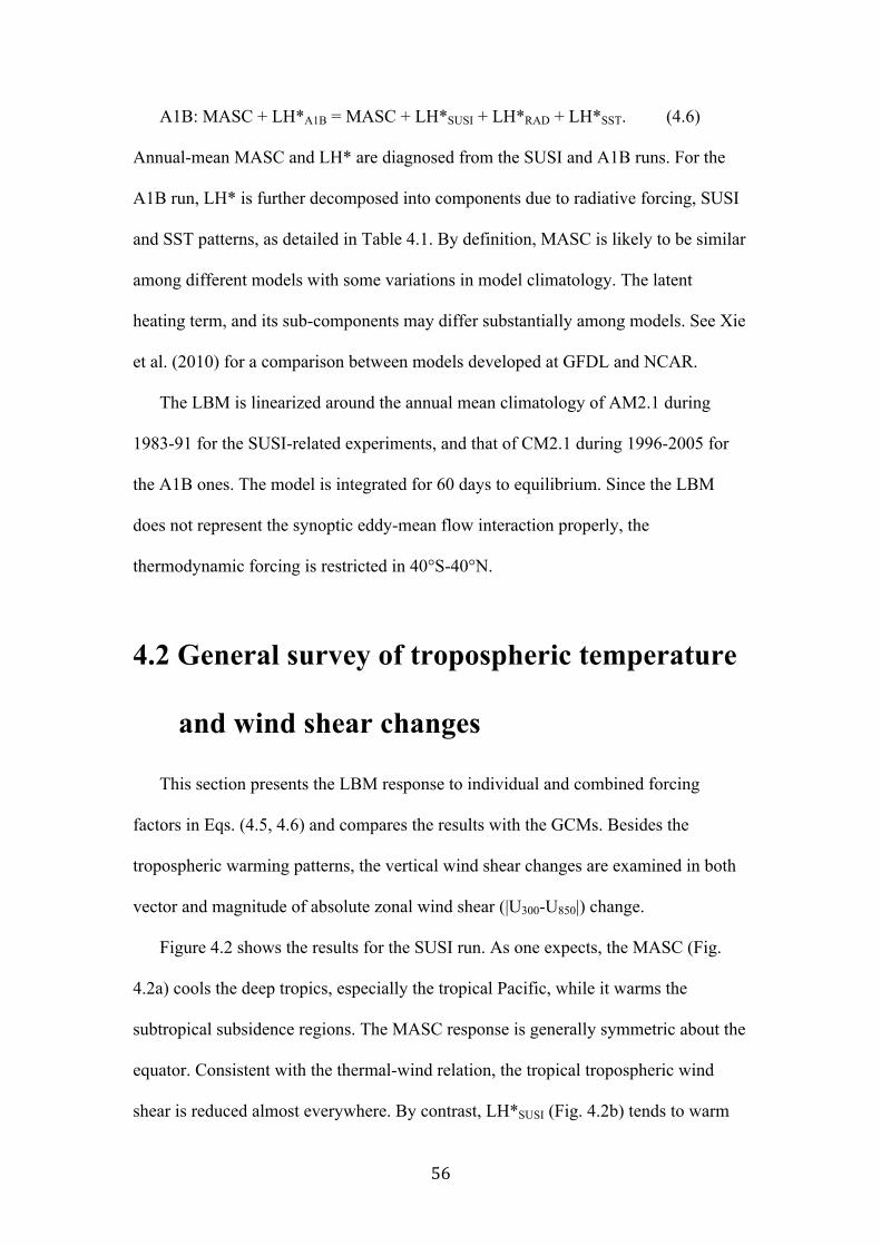
56
A1B: MASC + LH*A1B = MASC + LH*SUSI + LH*RAD + LH*SST. (4.6)
Annual-mean MASC and LH* are diagnosed from the SUSI and A1B runs. For the
A1B run, LH* is further decomposed into components due to radiative forcing, SUSI
and SST patterns, as detailed in Table 4.1. By definition, MASC is likely to be similar
among different models with some variations in model climatology. The latent
heating term, and its sub-components may differ substantially among models. See Xie
et al. (2010) for a comparison between models developed at GFDL and NCAR.
The LBM is linearized around the annual mean climatology of AM2.1 during
1983-91 for the SUSI-related experiments, and that of CM2.1 during 1996-2005 for
the A1B ones. The model is integrated for 60 days to equilibrium. Since the LBM
does not represent the synoptic eddy-mean flow interaction properly, the
thermodynamic forcing is restricted in 40°S-40°N.
4.2 General survey of tropospheric temperature
and wind shear changes
This section presents the LBM response to individual and combined forcing
factors in Eqs. (4.5, 4.6) and compares the results with the GCMs. Besides the
tropospheric warming patterns, the vertical wind shear changes are examined in both
vector and magnitude of absolute zonal wind shear (|U300-U850|) change.
Figure 4.2 shows the results for the SUSI run. As one expects, the MASC (Fig.
4.2a) cools the deep tropics, especially the tropical Pacific, while it warms the
subtropical subsidence regions. The MASC response is generally symmetric about the
equator. Consistent with the thermal-wind relation, the tropical tropospheric wind
shear is reduced almost everywhere. By contrast, LH*SUSI (Fig. 4.2b) tends to warm

57
the tropics and cool the subtropics, especially in the South Pacific, causing wind shear
to increase in the subtropical Pacific and the tropical Atlantic region of frequent
cyclone development (Vecchi and Soden 2007c). The MASC and LH*SUSI responses
oppose each other and the spatial correlation is -0.69 for tropospheric temperature and
-0.4 for wind shear (Table 4.2). In the central and eastern equatorial Pacific, however,
LH*SUSI reduces the wind shear, apparently due to the “upped-ante” cooling to the
west of the climatological equatorial cold tongue (Fig. 4.1a). LBM simulations forced
by observed diabatic heating have been very successful in capturing circulation
change associated with natural variability such as ENSO. If one was to do the same
for global warming as in the SUSI run, he/she would be surprised that the simulated
circulation change is almost opposite to the GCM results. This illustrates the
importance of MASC.
The combined MASC and LH*SUSI response (Fig. 4.2c) resembles the AM2.1
(SUSI) results (Fig. 4.2d), with spatial correlation for tropospheric temperature/wind
shear changes at r = 0.34/0.64. This illustrates the skills of LBM in simulating the
circulation response to global warming. The magnitude of LBM results is slightly
weaker than that of AM2.1, possibly due to the arbitrarily set damping and horizontal
diffusion. The tropospheric cooling in the mid-latitude South Pacific is not strong
enough in the LBM, possibly related to eddy effects. The peaks of subtropical
warming by LH*SUSI (Fig. 4.2b) are slightly shifted to lower latitudes than in AM2.1
(Fig. 4.2d), and the MASC (Fig. 4.2a) helps to adjust them to the right positions (Fig.
4.2c). The cooling over the Tibetan Plateau is due to the MASC (Figs. 4.2a, c, d)
associated with orographic convection anchored by the Himalayas and advected by
the westerly jet stream. The tropical Pacific wind shear is generally reduced (Figs.
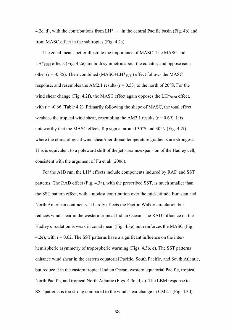
58
4.2c, d), with the contributions from LH*SUSI in the central Pacific basin (Fig. 4b) and
from MASC effect in the subtropics (Fig. 4.2a).
The zonal means better illustrate the importance of MASC. The MASC and
LH*SUSI effects (Fig. 4.2e) are both symmetric about the equator, and oppose each
other (r = -0.85). Their combined (MASC+LH*SUSI) effect follows the MASC
response, and resembles the AM2.1 results (r = 0.53) to the north of 20°S. For the
wind shear change (Fig. 4.2f), the MASC effect again opposes the LH*SUSI effect,
with r = -0.66 (Table 4.2). Primarily following the shape of MASC, the total effect
weakens the tropical wind shear, resembling the AM2.1 results (r = 0.69). It is
noteworthy that the MASC effects flip sign at around 30°S and 30°N (Fig. 4.2f),
where the climatological wind shear/meridional temperature gradients are strongest.
This is equivalent to a poleward shift of the jet streams/expansion of the Hadley cell,
consistent with the argument of Fu et al. (2006).
For the A1B run, the LH* effects include components induced by RAD and SST
patterns. The RAD effect (Fig. 4.3a), with the prescribed SST, is much smaller than
the SST pattern effect, with a modest contribution over the mid-latitude Eurasian and
North American continents. It hardly affects the Pacific Walker circulation but
reduces wind shear in the western tropical Indian Ocean. The RAD influence on the
Hadley circulation is weak in zonal mean (Fig. 4.3e) but reinforces the MASC (Fig.
4.2e), with r = 0.62. The SST patterns have a significant influence on the inter-
hemispheric asymmetry of tropospheric warming (Figs. 4.3b, e). The SST patterns
enhance wind shear in the eastern equatorial Pacific, South Pacific, and South Atlantic,
but reduce it in the eastern tropical Indian Ocean, western equatorial Pacific, tropical
North Pacific, and tropical North Atlantic (Figs. 4.3c, d, e). The LBM response to
SST patterns is too strong compared to the wind shear change in CM2.1 (Fig. 4.3d).

59
The comparison of LBM results with CM2.1 is greatly improved (Table 4.2) from
MASC+LH*SUSI (Fig. 4.2c) to MASC+LH*A1B (Fig. 4.3c). The reduction in wind
shear over the tropical Indian Ocean is a major difference between SUSI (Figs. 1.2a
and 4.2d) and A1B (Figs. 1.2b and 4.3d), due to both RAD and SST effects. Likewise
the increased wind shear in the eastern tropical North Pacific is due to the SST
patterns. The MASC effect is most pronounced in the Northern Hemisphere, helping
maintain the cooling in the deep tropics and the associated wind shear reduction in the
North Pacific (Figs. 4.2c, e and 4.3b, c, e). The combined MASC+LH*A1B effect
increases the correlation with CM2.1 by 0.2 compared to the LH*A1B effect.
The MASC effect is much weaker than LH in interannual variability of the
atmosphere, but the above analyses show that it is important in global warming.
Specifically, the MASC mechanism acts to reduce tropical tropospheric meridional
temperature gradients and zonal wind shear. Along with the “wet-get-wetter”
mechanism (Chou and Neelin 2004), the MASC is an important mechanism of pattern
formation when SST warming is spatially uniform.
4.3 Overturning circulations in LBM
This section examines the forcing factors for overturning circulation changes
based on LBM simulations and comparison with GCMs.
4.3.1 Walker circulation
Upper-tropospheric velocity potential (χ) was used to diagnose the large-scale
atmospheric circulation (Gastineau et al. 2009). χ at the 250 hPa level is calculated to

60
characterize the change of the Walker circulation, by solving the following Poisson
equation on the globe (Tanaka et al. 2004),
€
∇⋅ V = −Δχ,
where
€
V is wind velocity. Figures 4.4a-h show the horizontal distributions of the
changes in 250 hPa χ (color shading) and divergent wind (vectors) in response to
various forcing factors. The climatological mean (contours) features the Pacific
Walker circulation with divergence/convergence (negative/positive χ) on the
western/eastern basins.
The MASC (Fig. 4.4a) tends to reduce the divergence/upward motion over the
Indo-Pacific warm pool, by its adiabatic cooling effect illustrated in Fig. 4.1. By
contrast, LH*SUSI (Fig. 4.4b) induces divergence over the eastern Pacific, due to the
heating peak there (Fig. 4.1a), and weak convergence at 170°E (Fig. 4.4i), due to the
“upped-ante” mechanism. Even without any SST gradient, the MASC and LH*SUSI
act together to slow down the Walker circulation over the vast area of the Pacific
(Figs. 4.4e, f). High spatial correlation (r = 0.78, Table 4.3) appears between
MASC+LH*SUSI and AM2.1. χ on the equator (Fig. 4.4i), representing the Walker
circulation, shows that the MASC reduces the zonal wind between 130°E and 130°W,
while the LH*SUSI reduces it in 130°-90°W. The higher correlation with AM2.1 of
MASC (0.74) than of LH*SUSI (0.55) indicates the MASC effect is key to the success
of LBM simulation of the weakened Walker circulation (r = 0.87 for
MASC+LH*SUSI).
For changes in A1B, the RAD slightly strengthens the Walker circulation (Figs.
4.4c, j). The peak of SST warming in the mid-equatorial Pacific (Fig. 4.1b), contribute
to a divergence center at 175°E in the central Pacific (Fig. 4.4d, j), reducing the
Walker circulation over the western Pacific but accelerating it in the eastern basin.

61
Primarily maintained by the MASC, the zonal wind reduction of MASC+LH*A1B
extends to 140°W (Fig. 4.4g, j) and is almost identical to CM2.1 (Fig. 4.4h, j), with
very high spatial correlation (0.94) especially on the equator (0.97).
Thus, the MASC is very important for the weakening of the Walker circulation,
even more so in the A1B simulation. It has essential effect over the west-to-mid
equatorial Pacific. The SST contribution to χ is strong over the entire Pacific, but its
accelerating effect is opposed by the MASC to the west of 140°W. Considering SST
patterns of CM2.1 are among the strongest (spatial standard deviation is 0.24 K per K
tropical mean warming, as compared to the CMIP3 model ensemble of 0.17 ± 0.05 K
per K), the strong MASC effect explains that the weakening of the Walker cell is very
robust among the CMIP3 models (Vecchi and Soden, 2007a).
4.3.2 Hadley circulation
The Hadley circulation change is represented by the zonal-integrated meridional
mass stream function (ψ, Fig. 4.5), and by the zonal mean 250 hPa χ (Figs. 4.4k, l). ψ
is calculated as follows,
ψ =1g
V dp100 hPa
p∫ , (4.7)
where g is gravity and V is zonal-‐integrated meridional wind velocity. Figure 4.5
shows the climatological annual mean Hadley circulation in contours, which features
a clockwise/anticlockwise tropical cell (positive/negative values of ψ) in the
Northern/Southern Hemisphere, with upward motion over the ITCZ (~5°N) and
subsidence in the subtropics (20°-40°).
The MASC forces a significant weakening of the Hadley circulation (Figs. 4.5a
and 4.4k), while LH*SUSI accelerates it (Figs. 4.5b and 4.4k) at a reduced magnitude.

62
The combined effect follows the MASC patterns (r = 0.43 for ψ and 0.66 for χ) and is
quite similar (r ≥ 0.67) between the LBM (Figs. 4.5e and 4.4k) and AM2.1 (Figs. 4.5f
and 4.4k). Thus, the MASC is the major driver for the Hadley circulation reduction in
the AM2.1 SUSI experiment. Although the LH*SUSI effect is weak here, its sign is
always opposite to the MASC.
In response to GHG increase, the RAD effect causes a weak reduction in the
Hadley cell in the Northern Hemisphere (Figs. 4.5c and 4.4l), with the same sign as
the MASC. The SST patterns (specifically the equatorial peak, Fig. 4.1b) induce an
anomalous cell on either side of the equator (Fig. 4.5d), with a meridional scale of the
equatorial Rossby radius of deformation (~15°). This corresponds to an acceleration
of the Hadley cell near the equator in response to the equatorial peak in SST warming
(Liu et al. 2005; Xie et al. 2010). Because the SST warming is greater in the Northern
than the Southern Hemisphere (Fig. 4.1b), the Northern SST-induced equatorial cell is
weak, especially above 500 hPa, and the Hadley cell is reduced in the Northern off-
equatorial region. As a result, only the southern cell intensification is visible in the
upper troposphere (Fig. 4.4l).
The total effect of the four factors (MASC+LH*A1B, Fig. 4.5g) explains the
CM2.1 changes (Fig. 4.5h) quite well (r = 0.88). The Hadley cell weakens in the
Northern Hemisphere and accelerates in the Southern Hemisphere. For the Northern
Hemispheric cell, the SST-induced acceleration is offset by the LH*SUSI while both
the MASC and RAD effects contribute to the reduction. In the Southern Hemisphere,
the SST-induced cell dominates over the MASC+LH*SUSI effect, accelerating the
Hadley cell.
Figures 4.6 and 4.7 show the seasonal cycle of the Hadley circulation change. The
boreal summer is represented by mean during June-July-August (JJA), and the boreal
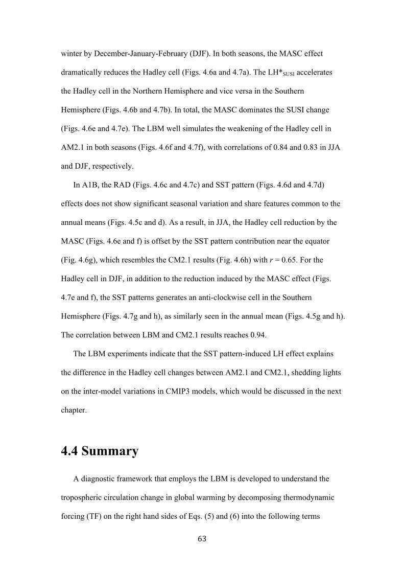
63
winter by December-January-February (DJF). In both seasons, the MASC effect
dramatically reduces the Hadley cell (Figs. 4.6a and 4.7a). The LH*SUSI accelerates
the Hadley cell in the Northern Hemisphere and vice versa in the Southern
Hemisphere (Figs. 4.6b and 4.7b). In total, the MASC dominates the SUSI change
(Figs. 4.6e and 4.7e). The LBM well simulates the weakening of the Hadley cell in
AM2.1 in both seasons (Figs. 4.6f and 4.7f), with correlations of 0.84 and 0.83 in JJA
and DJF, respectively.
In A1B, the RAD (Figs. 4.6c and 4.7c) and SST pattern (Figs. 4.6d and 4.7d)
effects does not show significant seasonal variation and share features common to the
annual means (Figs. 4.5c and d). As a result, in JJA, the Hadley cell reduction by the
MASC (Figs. 4.6e and f) is offset by the SST pattern contribution near the equator
(Fig. 4.6g), which resembles the CM2.1 results (Fig. 4.6h) with r = 0.65. For the
Hadley cell in DJF, in addition to the reduction induced by the MASC effect (Figs.
4.7e and f), the SST patterns generates an anti-clockwise cell in the Southern
Hemisphere (Figs. 4.7g and h), as similarly seen in the annual mean (Figs. 4.5g and h).
The correlation between LBM and CM2.1 results reaches 0.94.
The LBM experiments indicate that the SST pattern-induced LH effect explains
the difference in the Hadley cell changes between AM2.1 and CM2.1, shedding lights
on the inter-model variations in CMIP3 models, which would be discussed in the next
chapter.
4.4 Summary
A diagnostic framework that employs the LBM is developed to understand the
tropospheric circulation change in global warming by decomposing thermodynamic
forcing (TF) on the right hand sides of Eqs. (5) and (6) into the following terms

64
TF = MASC + LH*SUSI + LH*RAD + LH*SST.
The results demonstrate the LBM’s utility in global warming pattern studies to
quantify the relative importance of various forcing factors. Global warming features a
nearly horizontal-uniform increase of tropospheric temperature. The MASC is
important in tropical circulation adjustment, comparable in magnitude to the LH*SUSI
and SST pattern effects, while the RAD effect is much weaker.
Based on the LBM experiments, the questions raised in the beginning of this
chapter can be answered. The MASC warms the subsidence and cools the convective
regions, so that the subtropics are more warmed. The SST patterns also contribute to
the tropospheric warming patterns but this effect is overcome by the MASC in zonal
mean. The MASC weakens both the Hadley and Walker circulation, but the SST
patterns have significant influence, especially on the uncertainty of the Hadley
circulation change, as detailed below.
In response to a uniform SST increase without any gradient, the Walker
circulation weakens due to both the MASC and LH*SUSI effects in the western and
eastern Pacific, respectively. The SST patterns in CM2.1 significantly reduce the
Walker circulation in the western Pacific but accelerate it in the eastern basin.
Because the MASC effect is strong over a vast area of the equatorial Pacific, the
Walker circulation slow down is robust among the CMIP3 models under the A1B
scenario.
In response to a uniform SST warming, the Hadley circulation slow down due to
the MASC effect. In the A1B simulation with CM2.1, however, the slow down is
limited to the Northern Hemispheric cell while the Southern cell accelerates. The
LBM results show that this asymmetric response is due to SST patterns, specifically
an inter-hemispheric asymmetry with greater SST warming in the Northern than the

65
Southern Hemisphere. The meridional variations of SST warming in CM2.1 are
among the strongest of the CMIP3 models. In some coupled models with weak SST
patterns, e.g. the CCCMA CGCM3.1 T63, GISS AOM, MIROC3.2 Hires, and MRI
CGCM2.3 (not shown), the MASC effect to slow down the Hadley circulation in both
hemispheres can be stronger than the SST pattern effect, resulting in a weakened
Hadley circulation in both hemispheres (Fig. 5.4a).
During the seasonal march of the Hadley circulation, the MASC and SST pattern
effects are shown to be the major factors for the intensity change. As the MASC
makes strong contributions to the weakening of the Hadley cell in both seasons, the
SST pattern effect explains the difference between the SUSI and A1B changes seen in
the GCM simulations.
For the tropical wind shear and tropospheric temperature changes, the boreal
summer simulations by the LBM show similar skills to the annual mean ones in
reproducing GCM results. In the boreal winter, LBM’s simulation skills are much
lower. This seasonality appears consistent with the theory of Schneider et al. (2010).
An important parameter for this theory is the local Rossby number,
Ro = -ζ/f,
where ζ is relative vorticity, and f is the Coriolis parameter. When Ro → 1, the
angular momentum conservation degenerates and provides no constraint on the mean
meridional mass flux, and the tropical circulation change responds directly to the
thermal driving. When Ro → 0, circulation is dynamically constrained and change in
the eddy momentum flux divergence plays an important role. Figure 5 of Schneider et
al. (2010) shows that only in boreal summer the local Ro are larger than 0.5 in much
of the upper branch of the Hadley cell in both hemispheres, while in boreal winter, the

66
local Ro is smallest. The eddy effects (Lu et al. 2007; Schneider et al. 2010) are not
considered in this chapter but worth in-depth investigations.

67
Table 4.1. Descriptions of the LBM experiments.
Name Forcing Contribution
MASC MASC diagnosed from AM2.1 (SUSI) only SUSI/A1B
LH*SUSI LH* diagnosed from AM2.1 (SUSI) only SUSI/A1B
MASC+LH*SUSI MASC and LH* diagnosed from AM2.1 (SUSI) SUSI/A1B
LH*SST LH* of CM2.1 (A1B) - AM2.1 (SUSI) - RAD A1B
LH*A1B LH* diagnosed from CM2.1 (A1B) only A1B
MASC+LH*A1B MASC and LH* diagnosed from CM2.1 (A1B) A1B

68
Table 4.2. Spatial correlation coefficient (r, 40°S-40°N) of annual mean 300-850 hPa
averaged air temperature warming patterns/absolute zonal wind shear (ash) change
among LBM and GFDL models.
r (40°S-40°N) x-y / zm MASC LH*SUSI LH*SST MASC+
LH*SUSI MASC+LH*A1B
Tva*|AM2.1
0.14 0.19
0.13 0.09 ---- 0.34
0.53 ----
Uash’|AM2.1 0.21 0.70
0.48 -0.32 ---- 0.64
0.69 ----
Tva*|CM2.1
0.19 0.26
-0.16 -0.23
0.60 0.48
0.01 0.06
0.62 0.76
Uash’|CM2.1 0.11 0.01
0.15 0.08
0.43 0.59
0.24 0.07
0.61 0.55
Tva*|MASC ---- -0.69
-0.85 -0.37 -0.54 ---- ----
Uash’|MASC ---- -0.40 -0.66
-0.23 -0.37 ---- ----

69
Table 4.3. Spatial correlation coefficient (r, 40°S-40°N) of annual mean changes of
250 hPa velocity potential (χ) and meridional stream function (ψ) among LBM and
GFDL models.
r (40°S-40°N) x-y / em / zm MASC LH*SUSI LH*SST MASC+
LH*SUSI MASC+LH*A1B
χ |AM2.1 0.62 0.74 0.66
0.45 0.55 -0.48
---- 0.78 0.87 0.68
----
χ |CM2.1 -0.11 0.03 -0.20
0.68 0.67 0.48
0.57 0.65 0.81
0.54 0.53 -0.09
0.94 0.97 0.94
χ |MASC ---- -0.14 0.05 -0.81
-0.54 -0.48 -0.69
---- ----
ψ |AM2.1 0.43 0.08 ---- 0.67 ----
ψ |CM2.1 -0.25 0.45 0.62 0.14 0.88
ψ |MASC ---- -0.68 -0.65 ---- ----
em denotes equatorial mean (15°S-15°N).

70
Fig. 4.1. Annual mean distributions (a-f) of 300-850 hPa averaged terms in Eq. (4.3)
in 0.1 K day-1 (CI 0.05 K day-1; zero omitted), along with their equatorial means (g, h,
5˚S-5˚N) and zonal means (i, j) in SUSI and A1B runs. In (c) and (d), T* and CC
denote the warming patterns and circulation change terms, respectively. In (f), SH* is
unavailable in CM2.1 output, so instead, LWC* is plotted to show the relation
between QR* and LH*. In (h), (j), and hereinafter, LH* represents the combined effect
of LH* and QR* in A1B run. In (g)-(j), Sum means the summation of MASC, LH*
and CC to show their approximate balance (Eq. 4.4).

71
Fig. 4.2. 300-850 hPa averaged air temperature warming patterns (color shading, K),
wind shear (vectors, m s-1), and absolute zonal wind shear (contours, CI 0.5 m s-1;
zero omitted) changes in LBM forced by annual mean (a) MASC, (b) LH*SUSI, and (c)
MASC+LH*SUSI, compared with (d) AM2.1. (e), (f) are the zonal means of the
warming patterns and absolute shear change, respectively.

72
Fig. 4.3. 300-850 hPa averaged air temperature warming patterns (color shading, K),
wind shear (vectors, m s-1), and absolute zonal wind shear (contours, CI 0.5 m s-1;
zero omitted) changes in (a) RAD, LBM forced by annual mean (b) LH*SST, and (c)
MASC+LH*A1B, compared with (d) CM2.1. (e), (f) are the zonal means of the
warming patterns and absolute shear change, respectively.

73
Fig. 4.4. Annual mean changes of 250 hPa velocity potential (105 m2 s-1) distribution
(a-h, color shading) with the equatorial means (i, j) and zonal means (k, l). In (a)-(h),
vectors are the changes of divergent wind (m s-1), and contours (CI 20×105 m2 s-1;
zero omitted) show the mean velocity potential for reference.

74
Fig. 4.5. Annual mean changes of the Hadley circulation presented by the zonal-
integrated meridional stream function (color shading, 1010 kg s-1) with the contours
(CI 2×10¹⁰ kg s-1; zero omitted) showing the mean circulation for reference.

75
Fig. 4.6. Same as Fig. 4.5, but for JJA mean changes (CI 4×10¹⁰ kg s-1).

76
Fig. 4.7. Same as Fig. 4.6, but for DJF mean changes.

77
Chapter 5
Tropical overturning circulation change:
CMIP multi-model results
As is clear in Chapters 3 and 4, the MASC and SST patterns are both important
for atmospheric circulation change in the coupled model. MASC is responsible for the
slow-down of tropical circulation in SUSI, while SST patterns accounts much for the
inter-model uncertainty, especially for the Hadley circulation. This chapter
investigates what controls the response of tropical overturning circulation to global
warming in a large model ensemble, and the role of SST warming patterns in
particular. The results are presented based on three datasets: AGCM experiments to
understand the CMIP3 ensemble mean response (Section 2.3), CFMIP2 simulations as
part of CMIP5 (Section 2.2), and inter-model variability in CMIP3.
5.1 AGCM sensitivity experiments
Figure 5.1 illustrates the effect of CMIP3 ensemble mean SST patterns on the
Hadley circulation with the CAM experiments. The Hadley circulation is represented
by the zonal-integrated meridional mass streamfunction (Eq. 4.7). The CMIP3
ensemble-mean Hadley circulation change (Fig. 5.1a) features a weakening (slight
strengthening) in the Northern (Southern) Hemisphere. The CAM_A1B simulation

78
(Fig. 5.1b) captures the Northern Hemispheric changes well, but predicts a slight
reduction in the southern branch of the Hadley cell. Consistent with the MASC theory
of Ma et al. (2012), the SUSI effect (Fig. 5.1c) weakens the Hadley circulation in both
hemispheres. Because the southern branch of the Hadley cell is stronger in CAM than
in CMIP3 ensemble mean, the reduction may also be stronger, resulting in the
inconsistency between Figures 5.1a and b.
The T* effect (Fig. 5.1d) consists of two components: the equatorial peak (Fig.
5.1f) and inter-hemispheric asymmetry (Fig. 5.1e). The equatorial peak of the SST
warming enhances the Hadley cell on either side of the equator. The south-to-north
SST warming gradient causes a cross-equatorial circulation with an enhanced
southern Hadley cell and a reduced northern one.
In total, both the SUSI and T* effects contribute to the reduction of the Hadley
circulation in the Northern Hemisphere, but T* is the key factor for the enhancement
of the southern Hadley cell. This is consistent with the finding of Ma et al. (2012) that
the spread of cross-equatorial SST gradient explain much variability in the Southern
Hadley cell change among CMIP3 models, a point to be returned to in Section 5.3.
5.2 CMIP5-CFMIP2 simulations
The CFMIP2 experiments isolate the direct radiative, SUSI, and SST pattern
effects from the CMIP5 coupled models. The Hadley circulation is represented by the
zonal-integrated meridional mass streamfunction (ψ) at 500 hPa, and the Walker
circulation by equatorial (15°S-15°N) upper-tropospheric (250 hPa) velocity potential
(χ).
Figure 5.2 shows the 500-hPa ψ changes due to different factors. The SUSI effect
(Fig. 5.2a) tends to reduce the Hadley cell robustly. Since the MASC effect (Ma et al.

79
2012) is supposed to be identical among models, the inter-model variations come
mainly from LH. The RAD effect (Fig. 5.2c) is slight weakening, reinforcing the
SUSI. The equatorial peak in SST warming (Fig. 5.2b) accelerates the Hadley cell
near the equator. In the subtropics, the south-to-north warming gradient significantly
accelerates the southern cell. The combined effect (Fig. 5.2d) makes a robust slow-
down of the Hadley circulation in the northern subtropics. Whereas in the region near
and south of the equator, the opposing SUSI and SST pattern effects result in weak
and highly uncertain ensemble-mean change, subject to inter-model differences
brought by SST patterns and model physics. This is consistent with the CMIP3 results
(Fig. 5.4a) and CAM experiments (Fig. 5.1).
The 250-hPa χ (Fig. 5.3) shows a robust slow-down of the Pacific Walker
circulation in SUSI (Fig. 5.3a). The RAD (Fig. 5.3c) has a weak enhancing effect.
SST patterns (Fig. 5.3b) bring large uncertainty but do not offset the SUSI effect. As a
result, the Walker circulation slow-down is robust (Fig. 5.3d), similar to the CMIP3
results (Fig. 5.4b).
The MASC effect (Ma et al. 2012) in SUSI slows down both the Hadley (Fig. 5.2a)
and Walker (Fig. 5.3a) circulations. The RAD effect is weak (Figs. 5.2c and 5.3c).
The SST pattern effect (Figs. 5.2b and 5.3b) introduces considerable uncertainty to
both types of overturning circulations. The ensemble-mean effects of SST patterns are
quite different between them. T* contributes little to the Walker circulation (Fig. 5.3b)
so its slow-down remains robust (Figs. 5.3a, d). For the Hadley circulation by contrast,
the ensemble-mean T* counteracts the SUSI effect (Fig. 5.2b) and makes ψ flat and
uncertain in the southern subtropics and near the equator (Fig. 5.2d).
5.3 CMIP3 inter-model variability

80
This section investigates the SST pattern effect on inter-model variations of
overturning circulation changes in CMIP3. Figure 5.4 shows the climatology and
change of 500-hPa ψ (Fig. 5.4a) and 15°S-15°N averaged 250-hPa χ (Fig. 5.4b),
including both the CMIP3 ensemble mean and spread (shading). For the Hadley
stream function, there are large inter-model variations in 15°S-15°N, so large that
they can alter the sign of the Hadley circulation change in the southern subtropics and
equatorial region. In the northern subtropics, the Hadley cell slow-down is robust,
consistent with Figs. 5.1a and 5.2d. This asymmetry is due to the spatial variations in
ensemble mean SST warming as discussed above. The Pacific Walker circulation (Fig.
5.4b) shows a robust reduction, consistent with previous studies (Vecchi et al. 2006;
Vecchi and Soden 2007a). The inter-model variations appear on the same order of
magnitude as those for the Hadley circulation. Below investigates the cause of the
inter-model variability.
In order to examine the SST pattern effect on the inter-model variations of the
overturning circulation changes, two sets of inter-model SVD analyses are performed
among the CMIP3 GCMs. One is between the zonal mean SST and 500-hPa ψ, and
the other is between the equatorial SST and 250-hPa χ. Specifically, a conventional
SVD analysis is applied to 22 pairs of variables simulated by the 22 CMIP3 models.
The meridional SST modes (Fig. 5.5) feature the south-to-north gradient and the
equatorial peak (Ma et al. 2012). Both modes significantly influence ψ in the region
with high inter-model variability (Fig. 5.4a). The first SVD mode (Fig. 5.5a) is anti-
symmetric with positive/negative anomalous SST in the Northern/Southern
Hemisphere. This causes a cross-equatorial anticlockwise circulation between 15°S
and 15°N that represents an enhanced/weakened Hadley cell south/north of the
equator. The second mode (Fig. 5.5b) is symmetric and features an enhanced Hadley

81
circulation on either side of the equator (within 20°S-20°N), driven by the equatorial
peak of SST warming. The leading zonal modes (Fig. 5.6) represents inter-model
variability in zonal SST gradient across the Pacific, associated with changes in the
Walker circulation.
Then, the first two SVD modes of ψ and χ are removed from the inter-model
variability. Inter-model variations of the Hadley and the Pacific Walker circulations
are both dramatically reduced (Fig. 5.4), indicating that the SST warming patterns are
a major source of uncertainty in changes of overturning circulations. This does not
come as a surprise as the leading two modes explain 82% and 69% of the inter-model
variability in the Hadley (Fig. 5.5) and Walker (Fig. 5.6) circulations, respectively.
The residual uncertainty may be due to differences in model physics.
Figure 5.4 sheds light on the reason why the Hadley circulation change is not as
robust as the Walker circulation. Because inter-model variations in SST patterns
induce similar amount of uncertainty, the magnitude of the ensemble mean changes
becomes important. The slow-down of the Walker and northern Hadley cells are
robust because of large ensemble-mean changes. The Hadley circulation change near
and south of the equator is not robust, because of small ensemble-mean change. This
is illustrated more clearly by the CMIP5-CFMIP2 results (Figs. 5.2 and 5.3).
5.4 Summary
This chapter examines the changes of atmospheric overturning circulation in the
CMIP simulations. While the slow-down of the Walker circulation is robust across the
models, the change of the Hadley circulation is highly uncertain near and south of the
equator. As the MASC effect weakens both overturning circulations commonly in the
models, the SST patterns are a major source of the inter-model variability, accounting

82
for four fifth of the total variance. In ensemble mean, the SST pattern effect is weak
for the Walker circulation, so that the slow-down due to MASC is strong enough to
overcome the inter-model variability. The Hadley circulation change, by contrast, is
significantly affected by the SST patterns. In the northern subtropics, the south-to-
north gradient reinforces the MASC effect and results in a robust slow-down.
Whereas near and south of the equator, both the equatorial peak and meridional
gradient accelerate the Hadley cell, counteracting the MASC effect, so that the Hadley
circulation change is weak and subject to large inter-model variability induced by
differences in the SST patterns across the models.

83
Fig. 5.1. Annual mean changes of the Hadley circulation in (a) the CMIP3 ensemble
mean and (b-f) various CAM simulations. The Hadley circulation is represented by
the zonal-integrated meridional streamfunction (color shading, in 1010 kg s-1), with the
contours (CI: 2 × 10¹⁰ kg s-1; the zero contour omitted) showing the mean circulation
for reference.

84
Fig. 5.2. Annual mean changes of the 500-hPa zonal-integrated meridional
streamfunction (1010 kg s-1) in CMIP5-CFMIP2 simulations. The shading marks the
uncertainty (ensemble mean ± standard deviation) among the five models.

85
Fig. 5.3. Same as Fig. 5.2, but for the 15°S-15°N averaged 250-hPa velocity potential
(105 m2 s-1).

86
Fig. 5.4. Annual mean climatology and changes of the (a) 500-hPa zonal-integrated
meridional streamfunction (in 1010 kg s-1), and (b) 15°S-15°N averaged 250-hPa
velocity potential (in 105 m2 s-1) in CMIP3 A1B simulations. Gray/light red shading
marks the uncertainty (ensemble mean ± standard deviation) of the 22 GCMs in
climatology/change. The dark red shading marks the reduced uncertainty by removing
the first two SVD modes on SST. The figure is scaled by the climatology so that one
can compare the Hadley and Walker circulations.

87
Fig. 5.5. First two modes of the inter-model SVD analysis between the annual mean
changes of zonal mean SST patterns and 500-hPa zonal-integrated meridional
streamfunction among the 22 CMIP3 GCMs under the A1B scenario. Reproduced
from Ma et al. (2012).

88
Fig. 5.6. Same as Fig. 5.5, but for SST and 250-hPa velocity potential along the
equator, averaged in 5°S-5°N and 15°S-15°N, respectively.

89
Chapter 6
Conclusions
This study investigates the fundamental mechanisms controlling tropical regional
rainfall and tropospheric circulation changes in response to global warming and points
to the SST patterns as a major source of their inter-model variability. While large
uncertainties exist among the CMIP models, two robust mechanisms are found. One is
the MASC effect associated with tropical mean SST warming, which by definition is
identical among the models, acting to slow down the tropical circulation. And the
other is the “warmer-get-wetter” view among coupled models with SST change
patterns, casting the SST patterns (including two leading modes) as a major control on
regional precipitation change.
While SST increases everywhere in the tropics, precipitation change is to first
order variable in space. The model simulations show that if the SST increases
uniformly in space, the precipitation change follows a “wet-get-wetter” pattern.
However, in coupled models with increased GHG concentration, a “warmer-get-
wetter” pattern dominates. Although the SST patterns are only a fraction of the
tropical mean SST warming, it takes a major control on the regional precipitation
change through atmospheric circulation adjustments. Because equatorial waves flatten
the tropospheric warming to a value determined by tropical-mean SST warming, the
threshold for tropical convection rises and the SST pattern effect dominates the

90
rainfall response. In many parts of tropical oceans, convection is reduced despite an
increase in local SST because the local warming falls below the tropical average. In
other parts of the tropics where relative SST change is positive, precipitation
generally increases.
As illustrated in Figure 1.1, take any two global-warming simulations, and the
differences in projected rainfall change are obvious and substantial. Differences in
patterns of SST warming explains about one third of inter-model variability in tropical
rainfall change among CMIP3 models and one fourth in CMIP5 models.
Two major patterns reside in both ensemble mean and inter-model variations of
the CMIP3 and CMIP5 models. One is a meridional dipole mode, with a warmer
hemisphere anchoring enhanced rainfall and reduced trades. The other is a peak
warming along the equator, which is more ENSO like in CMIP5 than in CMIP3. Note
that the ensemble mean tends to underestimate the spatial variations. For instance, in
individual CMIP3 models, the spatial standard deviations of SST warming in 20°S-
20°N are 0.19 ± 0.04 K for a nominal 1K tropical-mean warming, considerably higher
than the ensemble mean (0.12 K). If nature evolves as one of the model realizations,
the importance of the SST change patterns would be more significant than what is
shown here for the ensemble mean.
Based on a series of LBM simulations, this study shows that the MASC
mechanism is crucial in weakening the tropical atmospheric circulation (including the
Walker, Hadley cells and vertical shear) and reducing the meridional temperature
gradients of the tropical troposphere. The MASC effect arises from adiabatic
cooling/heating due to the vertical advection by climatological upward/downward
motion on a background of global increase in static stability. MASC is an important
mechanism for circulation adjustment to global warming.

91
With the inclusion of MASC, the LBM is able to simulate the effects of various
forcing factors of global warming patterns. The MASC effect is shown to be
important in tropical circulation adjustment, comparable in magnitude to the SST
pattern effect. In interannual variability, the ratio of tropical mean/standard deviation
for SST anomaly drops to ~1/7 (see Introduction), and the MASC and LH*SUSI effects
become much weaker than the SST pattern effect, and the effect of SST pattern-
induced LH dominates the tropical circulation anomalies. This is a fundamental
distinction between interannual variability and global warming.
From the energetic point of view, the increased vertical gradients of potential
temperature in global warming enhance the efficiency of the Hadley cell in
transporting the dry static energy from the equator to the subtropics, assuming the
strength of the Hadley cell does not change. This is equivalent to the MASC
mechanism. Held and Soden (2006) shows that the increase of moisture convergence
(supplying the LH) is insufficient to overcome the dry energy divergence. Therefore,
more energy is transported poleward (Zelinka and Hartmann 2012), flattening the
tropical tropospheric meridional temperature gradients, reducing the tropical wind
shear, pushing the synoptic eddies poleward, expanding and weakening the Hadley
circulation. During the warm phase of the ENSO, enhanced poleward energy transport
is also found because of the wind change associated with enhanced SST gradient (Lu
et al. 2008). In global warming, SST pattern effects on energy transport need further
investigations but SST gradient change is much weaker than global mean warming.
The MASC, instead of being caused by circulation change, drives the winds to
respond differently from the ENSO with same sign of energy transport change.
In the CMIP ensemble simulations, both the MASC and SST pattern effects are
important for the Hadley and Walker circulation response to global warming. If the

92
SST warming were spatially uniform, the Hadley and Walker circulation would both
slow down as articulated in previous studies (Held and Soden 2006; Vecchi et al.
2006; Ma et al. 2012). The equatorial-peaked warming accelerates the Hadley
circulation on either side of the equator while the reduced warming in the Southern
Hemispheric accelerates the southern Hadley cell. As a result, the northern Hadley
cell shows a robust slow down while the Hadley circulation intensity change near and
south of the equator is weak in the ensemble mean and subject to large inter-model
variability. Uncertainty in SST warming patterns, dominated by the equatorial peak
and cross-equatorial gradient modes, accounts for a whopping 82% of inter-model
variability in Hadley circulation change among CMIP3 models. Compared to the
Hadley circulation, the SST pattern effect on Walker circulation is weak, and the
SUSI effect dominates. As a result, the slow-down of the Walker circulation is a
robust feature across the CMIP models.
This study shows that SST patterns are important for future climate change, in the
“warmer-get-wetter” pattern and Hadley circulation response. In addition, the SST
patterns can explain the inter-model variations in TC frequency response to global
warming (Zhao and Held 2012). The tropical SST effect is not limited to the tropics as
shifts in tropical convection and circulation have major remote effects on climate
change elsewhere, via atmospheric teleconnection (Shin and Sardeshmukh 2011) and
by affecting modes of climate variability (Collins et al. 2010; Zheng et al. 2010).
Recent observational studies reveal robust evidence on air-sea coupling associated
with slow-down of the Walker cell and coherent patterns of climate change over
tropical oceans (Tokinaga and Xie 2011a; Tokinaga et al. 2012a, 2012b). Innovative
model experimentations show that ocean-atmospheric interactions, specifically the
WES feedback, are indeed at work in the formation of major SST warming patterns

93
(Lu and Zhao 2012). The Bjerknes feedback might behave differently in CMIP3 and
CMIP5 models. To the extent that changes in surface winds and ocean circulation are
important for SST patterns, this study calls for investigations into ocean-atmosphere
interactions that shape SST and precipitation changes, which is demonstrated to be
important for inter-model variability (an important measure of uncertainty) in a large
model ensemble.

94
Chapter 7
Discussion and outlook
7.1 Impact of mean SST biases
The climatological SST biases in the coupled models from observations may
induce significant error in projections for global warming. This section examines the
impact of these biases on rainfall prediction and the MASC effect.
7.1.1 Effect of SST biases on precipitation change
This section examines the influence of SST biases on precipitation change in the 5
CMIP5 models under 1pctCO2 and AMIPFuture scenarios. The 1pctCO2 means
coupled model forced by CO2 increase at 1% per year until quadrupling. The
AMIPFuture experiment runs with AGCM forced by observational SST plus
ensemble-mean change in CMIP3.
Fig. 7.1 shows the biases of climatological SST and precipitation between coupled
models (1pctCO2) and observations (AMIP). Two errors in the coupled models stand
out, including a stronger equatorial cold tongue with further westward extension and
the double ITCZ with positive SST anomalies in the southeastern Pacific. This forms
a zonal dipole bias in precipitation with an eastward gradient.

95
Two methods can be adopted to estimate the biases of precipitation prediction in
the coupled models. One is based on the linear relationship between percentage
rainfall change and SST patterns, and the other by directly comparing with the AMIP
experiments.
From Eq. 3.1, one could derive the formula for rainfall change bias, i.e.,
∇δP =∇P α T * +β T( ) , (7.1)
where ∇ denotes the difference between coupled models and observations. Here the
AMIPFuture run is used to train the linear model (α = 56% K-1, and β = 6% K-1) and
the mean rainfall error in Fig. 7.1 is applied to calculate the bias in change. However,
this method cannot resolve non-linear processes actually involved (Fig. 3.3).
In addition, difference of rainfall change between 1pctCO2 and AMIPFuture
experiments can be used as an estimation of rainfall change bias. However, the SST
pattern change in these two scenarios is somewhat different (not shown), which may
interfere the bias signals.
Fig. 7.2 shows the rainfall change bias estimation by both methods compared with
AMIPFuture rainfall change. The rainfall change (Fig. 7.2a) features an equatorial
increase and subtropical reduction, as seen in the CMIP3 ensemble mean (Fig. 3.2).
Between Figs. 7.2b and c, robust patterns in rainfall change biases resemble the mean
biases (Fig. 7.1), i.e. the equatorial zonal dipole. However, because neither method is
accurate, the attempt here calls for experimental designs specifically for detecting the
rainfall change biases, e.g., AMIP tests with different SST climatology (coupled
models vs. observations) but same SST pattern change.
7.1.2 Influence of SST biases on MASC effect

96
As illustrated in Figures 4.1a and b, there is slight difference in the MASC forcing
between the SUSI and A1B, due to discrepancy in climatological vertical motion. The
large-scale vertical motion is basically determined by the SST distribution, so the
climatological SST biases have significant effect on this MASC difference.
Figures 7.3 and 7.4 show the influence of the SST biases on the MASC forcing
(Eq. 4.3) in the GFDL models and the atmospheric response to this bias in MASC
effect calculated by the LBM, respectively. The major large-scale pattern of the SST
biases (Fig. 7.3a) includes a westward extension of the equatorial cold tongue and a
2° northward shift of the ITCZ. The former reduces the MASC forcing (Figs. 4.1a and
b) in the western equatorial Pacific (Fig. 7.3c) and results in a slightly weaker slow-
down of the Walker circulation (Fig. 7.4b) in A1B than in SUSI. The latter (Fig. 7.3b)
enhances the Hadley circulation a bit to the north of the equator (Fig. 7.4c). The
tropospheric temperature pattern due to the MASC bias includes a zonal dipole over
the South Pacific, along with wind shear reduction over the southeastern Pacific and
South America and enhancement in the equatorial Atlantic (Fig. 7.4a).
7.2 MASC in observations (AMIP)
Chapters 4 and 5 illustrate the importance of the MASC effect to atmospheric
circulation change in global warming. However, the analyses are limited to models for
future climate prediction. The section will examine the MASC effect in observations
(based on AMIP experiment with GFDL AM2.1 forced with observed SST), taking
the Walker circulation as an example. The MASC effect is calculated according to Eq.
(4.4) with the mean pressure velocity and anomaly of potential temperature in the
AMIP experiment. An EOF analysis is applied to separate the forcing patterns and
temporal trend. The latter is then compared with the Walker circulation change in the

97
AMIP runs and observations, which is represented by an index defined as the anomaly
of the surface zonal wind averaged in 5°S-5°N, 140°E-80°W.
The AMIP experiment with GFDL AM2.1 is forced with monthly SST and sea ice
of HadISST. The experiment consists of 9 members for 1950-2010 and the ensemble
and annual mean is shown here. Greenhouse gases, aerosols, ozone concentration,
land cover and solar radiation are fixed to 1990 climatological values.
The observed surface wind used here is the wave and anemometer-based sea-
surface wind (WASWind) dataset (Tokinaga and Xie 2011b). This new dataset
combines ship observations of surface wind velocity and wind wave height archived
in the International Comprehensive Ocean-Atmosphere Data Set (ICOADS) to correct
the spurious upward trend due to increases in anemometer height. The dataset is at a
monthly resolution of 4° by 4° from 1950 to 2009. It substantially reduces the upward
trend in wind speed through height-correction for anemometer-measured winds,
rejection of spurious Beaufort winds, and use of estimated winds from wind wave
height. It has been utilized for climate trend analysis (Tokinaga et al. 2012a).
Figure 7.5 shows the results. The MASC forcing patterns (Fig. 7.5a) are identical
to those in Figure 4.1a, with cooling in the convective regions and warming in the
subtropics. In temporal evolution (Fig. 7.5b), the long-term weakening of the Walker
circulation is observed in the WASWind, consistent with the MASC forcing.
However, the AMIP wind is much weaker than the WASWind during 1950-1975,
possibly due to the bias in patterns of SST forcing (Tokinaga et al. 2012a, 2012b).
The interannual variability of the two wind data agrees qualitatively and is
inconsistent and much stronger than that in MASC, providing evidence for the scale
analysis in Section 4.1.2 that MASC is much weaker than SST pattern effect in
interannual variability. In both wind datasets, the Walker circulation strengthens

98
during the last two decades, but this is irrelevant to the MASC forcing, indicating the
importance of other mechanisms, such as the decadal variation of the SST patterns.
7.3 Feedback processes stabilizing SST warming
Global warming involves climate feedback processes determining SST and
associated circulation changes. Detailed examination of these feedbacks is necessary
for better understanding the magnitude and form of such changes, in both global mean
and regional patterns. Namely, positive feedbacks include the water vapor feedback
enhancing the global SST warming, the WES feedback contributing to the inter-
hemispheric gradient, and the Bjerknes feedback forming the eastern equatorial
Pacific warming peak. Negative feedbacks include the Newtonian cooling in surface
latent heating and longwave radiation.
Specifically over the equatorial cold tongue and in the subtropics, low-cloud
feedbacks are important. As SST warms, water vapor increases and the atmosphere
stabilizes, which increases the low-cloud amount in these regions. This triggers both
longwave and shortwave feedbacks. The increased downward longwave cloud
radiation enhances SST warming but reduced shortwave radiation cools the surface.
Thus, whether the total low-cloud feedback is positive or negative depends on the
warming/cooling rates in specific regions. This open question needs further
investigation.
7.4 Changes of sea level and ocean circulation
SST patterns and associated surface wind changes may have significant influence
on regional patterns of sea level and ocean circulation changes (Timmermann et al.

99
2010). For instance, reduced SST warming in the South Pacific than on the equator
and in the North Pacific triggers the WES feedback that enhances trades in the South
Pacific. The resulted wind curl generates Ekman pumping/suction in the
southwestern/northeastern South Pacific, and hence anomalous sea level
rising/sinking. The geostrophic flow forced by this pattern of sea level change would
probably be along the wind direction. The regime of coupled response from SST
change patterns to atmospheric feedback and hence dynamical ocean response needs
to be investigated in future study.

100
Fig. 7.1. Ensemble-mean biases of climatological SST (contours, CI 0.5 K; zero
omitted) and precipitation (color shading, mm day-1) between 1pctCO2 and AMIP
experiments in CMIP5.

101
Fig. 7.2. Comparison between ensemble-mean precipitation change based on
observational SST and biases in the coupled models in CMIP5. (a) Rainfall change in
AMIPFuture run. (b) Biases in rainfall change predicted by the linear regression (Eq.
7.1). (c) Difference of rainfall change between 1pctCO2 and AMIPFuture
experiments.

102
Fig. 7.3. (a) Horizontal distribution of the difference in 300-850 hPa averaged MASC
forcing term (Eq. 4.3, in 0.1 K day-1) between SUSI and A1B runs with AM/CM2.1,
along with the (b) zonal mean, and (c) equatorial mean (5˚S-5˚N).

103
Fig. 7.4. Difference in atmospheric response to the MASC forcing between SUSI and
A1B calculated in LBM. (a) 300-850 hPa averaged air temperature warming patterns
(color shading, K), wind shear (vectors, m s-1), and absolute zonal wind shear
(contours, CI 0.5 m s-1; zero omitted). (b) 250-hPa velocity potential (color shading,
105 m2 s-1) with divergent wind (vectors, m s-1). Contours (CI 20×105 m2 s-1; zero
omitted) show the mean velocity potential for reference. (c) Zonal-integrated
meridional stream function (color shading, 1010 kg s-1) with the contours (CI 2×10¹⁰
kg s-1; zero omitted) showing the mean circulation for reference.

104
Fig. 7.5. EOF (a) and PC (b; black) of the MASC forcing in AMIP experiment with
GFDL AM2.1. The PC is compared with the Walker circulation index in the AMIP
experiment (blue) and observations (red) with 9 years running mean.

105
References
Bellouin, N., and Coauthors, 2011: Aerosol forcing in the Climate Model
Intercomparison Project (CMIP5) simulations by HadGEM2-ES and the role of
ammonium nitrate. J. Geophys. Res., 116, D20206, doi:10.1029/2011JD016074.
Betts, A. K., 1998: Climate-convection feedbacks: Some further issues. Climatic
Change, 39, 35-38.
Betts, A. K., and W. Ridgway, 1989: Climatic equilibrium of the atmospheric
convective boundary layer over a tropical ocean. J. Atmos. Sci., 46, 2621-2641.
Bretherton, C., and A. Sobel, 2003: The Gill model and the weak temperature gradient
approximation. J. Atmos. Sci., 60, 451–460.
Cess, R. D., and Coauthors, 1990: Intercomparison and interpretation of cloud-climate
feedback processes in 19 atmospheric general circulation Models. J. Geophys.
Res., 95, 16601-16615.
Chou, C., and J. D. Neelin, 2004: Mechanisms of global warming impacts on regional
tropical precipitation. J. Climate, 17, 2688-2701.
Chou, C., C.-A. Chen, P.-H. Tan, and K. T. Chen, 2012: Mechanisms for global
warming impacts on precipitation frequency and intensity. J. Climate, 25, 3291–
3306.
Chou, C., J. D. Neelin, C.-A. Chen, and J.-Y. Tu, 2009: Evaluating the “rich-get-
richer” mechanism in tropical precipitation change under global warming. J.
Climate, 22, 1982-2005.

106
Collins, M. and coauthors, 2010: The impact of global warming on the tropical Pacific
Ocean and El Niño. Nat. Geosci., 3, 391-397.
Collins, W. D., and Coauthors, 2006: The formulation and atmospheric simulation of
the Community Atmosphere Model: CAM3. J. Climate, 19, 2144–2161.
de Szoeke, and S.-P. Xie, 2008: The tropical eastern Pacific seasonal cycle:
Assessment of errors and mechanisms in IPCC AR4 coupled ocean-atmosphere
general circulation models. J. Climate, 20, 2573–2590.
Delworth, T. L., and Coauthors, 2006: GFDL’s CM2 global coupled climate models.
Part I: Formulation and simulation characteristics. J. Climate, 19, 643–674.
Frierson, D. M. W., J. Lu, and G. Chen, 2007: Width of the Hadley cell in simple and
comprehensive general circulation models. Geophys. Res. Lett., 34, L18804,
doi:10.1029/2007GL031115.
Gastineau, G., L. Li, and H. Le Treut, 2009: The Hadley and Walker circulation
changes in global warming conditions described by idealized atmospheric
simulations. J. Climate, 22, 3993–4013.
GFDL Global Atmospheric Model Development Team, 2004: The new GFDL global
atmosphere and land model AM2/LM2: Evaluation with prescribed SST
simulations. J. Climate, 17, 4641–4673.
Gill, A. E., 1980: Some simple solutions for heat-induced tropical circulation. Quart.
J. Roy. Meteorol. Soc., 106, 447-462.
Held, I. M., and B. J. Soden, 2006: Robust responses of the hydrological cycle to
global warming. J. Climate, 19, 5686–5699.
Held, I. M., T. L. Delworth, J. Lu, K. L. Findell, and T. R. Knutson, 2005: Simulation
of Sahel drought in the 20th and 21st centuries. Proc. Natl. Acad. Sci., 102,
17891-17896.

107
Hu, Y., and Q. Fu, 2007: Observed poleward expansion of the Hadley circulation
since 1979. Atmos. Chem. Phys., 7, 5229-5236, doi:10.5194/acp-7-5229-2007.
Johanson, C. M., and Q. Fu, 2009: Hadley cell widening: Model simulations versus
observations. J. Climate, 22, 2713-2725.
Johnson, N. C., and S.-P. Xie, 2010: Changes in the sea surface temperature threshold
for tropical convection. Nat. Geosci., 3, 842-845, doi:10.1038/ngeo1008.
Knutson, T. R., and S. Manabe, 1995: Time-mean response over the tropical Pacific
to increased CO2 in a coupled ocean-atmosphere model. J. Climate, 8, 2181-2199.
Knutson, T. R., J. J. Sirutis, S. T. Garner, G. A. Vecchi, and I. M. Held, 2008:
Simulated reduction in Atlantic hurricane frequency under twenty-first-century
warming conditions. Nat. Geosci., 1, 359-364.
Leloup, J., and A. Clement, 2009: Why is there a minimum in projected warming in
the tropical North Atlantic Ocean? Geophys. Res. Lett., 36, L14802,
doi:10.1029/2009GL038609.
Lindzen, R. S., 1990: Some coolness concerning global warming. Bull. Amer. Meteor.
Soc., 71, 288-299.
Liu, Z., S. Vavrus, F. He, N. Wen, and Y. Zhong, 2005: Rethinking tropical ocean
response to global warming: The enhanced equatorial warming. J. Climate, 18,
4684–4700.
Lu, J., and B. Zhao, 2012: The oceanic feedback in the climate response to doubling
CO2. J. Climate, in press.
Lu, J., G. Chen, and D. M. W. Frierson, 2008: Response of the zonal mean
atmospheric circulation to El Nino versus global warming. J. Climate, 21, 5835-
5851.

108
Lu, J., G. A. Vecchi, and T. Reichler, 2007: Expansion of the Hadley cell under
global warming. Geophys. Res. Lett., 34, L06805, doi:10.1029/2006GL028443.
Ma, J., S.-P. Xie, and Y. Kosaka, 2012: Mechanisms for tropical tropospheric
circulation change in response to global warming. J. Climate, 25, 2979-2994.
Matsuno, T., 1966: Quasi-geostrophic motions in the equatorial area. J. Met. Soc.
Japan, 44, 25-42.
Meehl, G. A., and Coauthors, 2007: The WCRP CMIP3 multimodel dataset: A new
era in climate change research. Bull. Amer. Meteor. Soc., 88, 1383-1394.
Muller, C. J., and P. A. O’Gorman, 2011: An energetic perspective on the regional
response of precipitation to climate change. Nature Clim. Change, 1, 266-271,
doi:10.1038/nclimate1169.
Neelin, J. D., C. Chou, and H. Su, 2003: Tropical drought regions in global warming
and El Nino teleconnections. Geophys. Res. Lett., 30, 2275,
doi:10.1029/2003GLO018625.
Ringer, M. A., and Coauthors, 2006: Global mean cloud feedbacks in idealized
climate change experiments. Geophys. Res. Lett., 33, L07718,
doi:10.1029/2005GL025370.
Rodwell, M. J., and B. J. Hoskins, 1996: Monsoons and the dynamics of deserts.
Quart. J. Roy. Meteor. Soc., 122, 1385–1404, doi:10.1002/qj.49712253408.
Schneider, T., P. A. O’Gorman, and X. J. Levine, 2010: Water vapor and the
dynamics of climate changes, Rev. Geophys., 48, RG3001,
doi:10.1029/2009RG000302.
Seager, R., and R. Murtugudde, 1997: Ocean dynamics, thermocline adjustment and
regulation of tropical SST. J. Climate, 10, 521–534.

109
Seager, R., and Coauthors, 2007: Model projections of an imminent transition to a
more arid climate in southwestern North America. Science, 316, 1181-1184.
Seager, R., N. Naik, and G. A. Vecchi, 2010: Thermodynamic and dynamic
mechanisms for large-scale changes in the hydrological cycle in response to
global warming. J. Climate, 23, 4651-4668.
Shin, S. I., and P. D. Sardeshmukh, 2011: Critical influence of the pattern of tropical
ocean warming on remote climate trends. Clim. Dyn.. 36, 1577-1591.
Sobel, A., 2010: Raised bar for rain. Nat. Geosci., 3, 821–822, doi:10.1038/ngeo1025.
Sobel, A., and S. Camargo, 2011: Projected future changes in tropical summer climate.
J. Climate, 24, 473-487.
Tanaka, H. L., N. Ishizaki, and A. Kitoh, 2004: Trend and interannual variability of
Walker, monsoon and Hadley circulations defined by velocity potential in the
upper troposphere. Tellus, 56A, 250–269.
Thomson, A. M., and Coauthors, 2011: RCP4.5: a pathway for stabilization of
radiative forcing by 2100. Climatic Change, 109, 77-94, doi:10.1007/s10584-011-
0151-4.
Timmermann, A., S. McGregor, and F.-F. Jin, 2010: Wind effects on past and future
regional sea-level trends in the southern Indo-Pacific, J. Climate, 23, 4429-4437.
Tokinaga, H., and S.-P. Xie, 2011a: Weakening of the equatorial Atlantic cold tongue
over the past six decades. Nat. Geosci., 4, 222-226.
Tokinaga, H., and S.-P. Xie, 2011b: Wave and Anemometer-based Sea Surface Wind
(WASWind) for climate change analysis. J. Climate, 24, 267-285.
Tokinaga, H., S.-P. Xie, A. Timmermann, S. McGregor, T. Ogata, H. Kubota, and Y.
M. Okumura, 2012a: Regional patterns of tropical Indo-Pacific climate change:
Evidence of the Walker Circulation weakening. J. Climate, 25, 1689-1710.

110
Tokinaga, H., S.-P. Xie, C. Deser, Y. Kosaka, and Y. M. Okumura, 2012b: Slowdown
of the Walker circulation driven by tropical Indo-Pacific warming. Nature,
doi:10.1038/nature11576, in press.
Vecchi, G. A., and B. J. Soden, 2007a: Global warming and the weakening of the
tropical circulation. J. Climate, 20, 4316–4340.
Vecchi, G. A., and B. J. Soden, 2007b: Effect of remote sea surface temperature
change on tropical cyclone potential intensity. Nature, 450, 1066-1070.
Vecchi, G. A., and B. J. Soden, 2007c: Increased tropical Atlantic wind shear in
model projections of global warming. Geophys. Res. Lett., 34, L08702,
doi:10.1029/2006GL028905.
Vecchi, G. A., B. J. Soden, A. T. Wittenberg, I. M. Held, A. Leetmaa, and M. J.
Harrison, 2006: Weakening of tropical Pacific atmospheric circulation due to
anthropogenic forcing. Nature, 441, doi:10.1038/nature04744.
Vecchi, G. A., K. L. Swanson, and B. J. Soden, 2008: Whither hurricane activity?
Science, 322, 687-689.
Watanabe, M., and F.-F. Jin, 2004: Dynamical prototype of the Arctic Oscillation as
revealed by a neutral singular vector. J. Climate, 17, 2119-2138.
Watanabe, M., and M. Kimoto, 2000: Atmosphere-ocean thermal coupling in the
North Atlantic: A positive feedback. Quart. J. R. Met. Soc., 126, 3343-3369.
Watanabe, M., and M. Kimoto, 2001: Corrigendum. Quart. J. R. Met. Soc., 127, 733-
734.
Wentz, F. J., L. Ricciardulli, K. Hilburn, and C. Mears, 2007: How much more rain
will global warming bring? Science, 317, 233-235.

111
Wittenberg, A. T., A. Rosati, N.-C. Lau, and J. J. Ploshay, 2006: GFDL’s CM2 global
coupled climate models. Part III: Tropical Pacific climate and ENSO. J. Climate,
19, 698–722.
Xie, S.-P., and S. G. H. Philander, 1994: A coupled ocean-atmosphere model of
relevance to the ITCZ in the eastern Pacific. Tellus, 46A, 340-350.
Xie, S.-P., C. Deser, G. A. Vecchi, J. Ma, H. Teng, and A. T. Wittenberg, 2010:
Global warming pattern formation: Sea surface temperature and rainfall. J.
Climate, 23, 966-986.
Zelinka, M. D., and D. L. Hartmann, 2012: Climate feedbacks and their implications
for poleward energy flux changes in a warming climate. J. Climate, 25, 608–624.
Zhang, X., and Coauthors, 2007: Detection of human influence on twentieth-century
precipitation trends. Nature, 448, 461-465, doi:10.1038/nature06025.
Zhao, M., and I. M. Held, 2012: TC-permitting GCM simulations of hurricane
frequency response to sea surface temperature anomalies projected for the late
21st Century. J. Climate, 25, 2995-3009.
Zheng, X.-T., S.-P. Xie, G. A. Vecchi, Q. Liu, and J. Hafner, 2010: Indian Ocean
dipole response to global warming: Analysis of ocean-atmospheric feedbacks in a
coupled model. J. Climate, 23, 1240-1253.