dynamics of disease transmission networksdynamics of disease transmission networks winfried just...
TRANSCRIPT

Dynamics of Disease Transmission Networks
Winfried JustDepartment of Mathematics
Ohio University
Presented at the workshopTeaching Discrete and Algebraic Mathematical Biology to
UndergraduatesMBI, Columbus, OH, July 31, 2013
Winfried Just at OU Disease Transmission Networks

What processes are we modeling?
We are interested in diseases that are triggered when infectiousagents such as viruses or bacteria (called microparasites) enter theorganism of a host (human, animal, plant).
We are not interested here in the actual changes that the diseasecauses in the organism of the host, or how the infectious agentsmultiply within the host. We only care about how the diseasespreads between hosts of a given population.
In this lecture we will focus on diseases whose transmission requiresdirect contact (of a certain type) between hosts, as opposed todiseases that require a third type of organisms, called vectors fortransmission between hosts (mosquitoes in the case of malaria), ordiseases where the infectious agents are taken up from the sharedenvironment of the hosts (drinking water in the case of cholera).
Ohio University – Since 1804 Department of Mathematics
Winfried Just at OU Disease Transmission Networks

Which questions are we trying to answer?
If some disease agents are introduced into a population ofhosts that have not previously been exposed to the disease,will an epidemic result? That is, should we expect that asignificant fraction of hosts in the population will eventuallyget infected?
If an epidemic does result, what proportion of hosts will beinfected? The proportion of hosts that will be infected atsome (not necessarily the same) time during the epidemic iscalled the final size (of the epidemic).
What control measures are most effective in either preventingan epidemic or reducing the final size as much as possible?
Possible control measures include vaccination, quarantine,culling (for animal and plant diseases), or behaviormodifications (for human diseases).
Ohio University – Since 1804 Department of Mathematics
Winfried Just at OU Disease Transmission Networks

When is a mathematical model good (enough)?
Our goal is to construct mathematical models that give us correctanswers to the questions on the previous slide. For that, we needthe model to:
Give us answers in the first place. Thus the model needs to besimple enough to be tractable either by mathematical analysisor computer simulations.
Be sufficiently realistic. It needs to take into accountsufficiently many biological details that influence the dynamicsso as to make reasonably correct predictions.
Be based on data that we actually can collect.
This may be too much to ask for. In practice, we may not knowwhether a given model is sufficiently realistic. But it is sometimespossible to study the mathematical problem of how more detailed,or finer-grained models relate to simplified coarser-grained models.
Ohio University – Since 1804 Department of Mathematics
Winfried Just at OU Disease Transmission Networks

What happens to a host during a disease?
Since we only aim at modeling the dynamics between hosts, weonly make the following assumptions about the disease that getstransmitted to host number i at time T i
E , which stands for thetime of exposure:
All (potential) hosts start out being susceptible to the disease(at times t < T i
E ).At all times T i
E ≤ t < T iI the host will not (yet) be able to
infect others.At all times t with T i
I ≤ t < T iR ≤ ∞ the host will be
infectious, that is, will transmit the disease with positiveprobability during contacts with susceptible hosts.At all times t ≥ T i
R the host will neither be infectious norsusceptible.
We are not assuming that T iI marks the onset of symptoms of the
disease. Neither does T iR always mark their cessation.
What happens at time T iR? What kind of diseases do not
satisfy the above assumptions?Ohio University – Since 1804 Department of Mathematics
Winfried Just at OU Disease Transmission Networks

The building blocks of disease models: compartments
Let’s summarize:
T iE is time of exposure of host number i .
T iI is time of onset of infectiousness of host number i .
T iR is time of removal of host number i , which means the host
number i either dies from the disease or acquires permanentimmunity at time T i
R .
This suggests a partition of host population at time t into up tofour compartments:S comprises all susceptible hosts (for which T i
E > t),E comprises all exposed hosts with T i
E ≤ t < T iI ),
I comprises all infectious hosts with T iI ≤ t < T i
R , andR comprises all removed hosts with T i
R ≤ t.
Ohio University – Since 1804 Department of Mathematics
Winfried Just at OU Disease Transmission Networks

SEIR-models
If all four compartments are considered, we get an SEIR-model.
Ohio University – Since 1804 Department of MathematicsWinfried Just at OU Disease Transmission Networks

SIR-models
The simplifying assumption T iE = T i
I eliminates theE -compartment and we get an SIR-model.
Ohio University – Since 1804 Department of Mathematics
Winfried Just at OU Disease Transmission Networks

SI -models
If in addition T iR =∞, then the R-compartment becomes
redundant and we get an SI -model.
Ohio University – Since 1804 Department of Mathematics
Winfried Just at OU Disease Transmission Networks

SIS-models
If we assume instead that at time T iR hosts recover and become
susceptible to reinfection instead of acquiring immunity, then weget an SIS-model.
Ohio University – Since 1804 Department of Mathematics
Winfried Just at OU Disease Transmission Networks

Four basic types of compartment models
S comprises all susceptible hosts (for which T iE > t),
E comprises all exposed hosts with T iE ≤ t < T i
I ),I comprises all infectious hosts with T i
I ≤ t < T iR , and
R comprises all removed hosts with T iR ≤ t.
The times T iE ,T
iI ,T
iR are specific to each host. Membership in the
compartments changes over time, and we can think of hostsmoving (but not in space!) from S to E to I to R.
The above is called an SEIR-model.The simplifying assumption T i
E = T iI eliminates the
E -compartment and gives an SIR-model.If in addition T i
R =∞, then the R-compartment becomesredundant and we get an SI -model.If we assume instead that T i
E = T iI and at time T i
R hostssimply recover and become susceptible to reinfection insteadof acquiring immunity, then we get an SIS-model.
Can you think of other types of meaningful compartmentmodels?Ohio University – Since 1804 Department of Mathematics
Winfried Just at OU Disease Transmission Networks

Are compartments good enough for our modeling?
Let us see whether we can translate our guiding questions intocompartmentalese.Assume an SIR-model. Consider a population of N individuals, allinitially in S , and assume K of them become infected from outsidesources at time TE , where K � N. Now let the disease run itscourse, and considerF (K ,N) = limt→∞
N − #S(t)N .
This limit is the final size, i.e. fraction of hosts that eventuallyexperience infection.
There is danger of an epidemic unless for fixed K we havelimN→∞ F (K ,N) = 0, which would mean that the disease willaffect only a negligible fraction of a large population.
How would vaccination at time Tv < TE of a fraction r ofhosts translate into compartmentalese?As moving rN hosts into R at time Tv .Compartmentalese seems to be a convenient language for us.Ohio University – Since 1804 Department of Mathematics
Winfried Just at OU Disease Transmission Networks

Compartment-based ODE models
In the remainder of this talk we will ignore theE -compartment and assume that the onset of infectiousnesscoincides with the time of exposure, that is, T i
I = T iE .
We will moreover assume that the population size N is fixed,which ignores demographics, that is, births, deaths fromunrelated causes, immigration and emigration.
In the resulting ODE models the state of the population isrepresented by three variables S , I , and R. These variablescould either represent the proportions of hosts in therespective compartments, or their numbers.
In order to make the use of derivatives somewhat respectable,one can think of population size being expressed in units of athousand or a million individuals so that at least somefractional values of the variables make sense.
Ohio University – Since 1804 Department of Mathematics
Winfried Just at OU Disease Transmission Networks

Basic ODE versions of the SI -, SIR- and SIS-models
SI -model:
dSdt = −βSIdIdt = βSI
SIS-model:
dSdt = −βIS + αIdIdt = βIS − αI
SIR-model:
dSdt = −βISdIdt = βIS − αIdRdt = αI
The rate of infection β may or may not depend on N; the removalrate α is always independent of N.Ohio University – Since 1804 Department of Mathematics
Winfried Just at OU Disease Transmission Networks

What do the ODE models predict?
These ODE models are easy to study analytically.
If S(0), I (0) > 0, then the SI -model predicts that dIdt > 0 at
all times and limt→∞ S(t) = 0, so the whole population willeventually be infected.
Since S = N − I , the SIS-model simplifies to the logisticgrowth modeldIdt = βI (N − I )− αI = βI (N − α
β − I ),which predicts both a disease-free equilibrium I ∗ = 0 and anendemic equilibrium I ∗∗ = N − α
β .
The SIR-model allows both for predicting whether or not anepidemic will occur and for predicting its final size if it does.
Would the final size be 1 if β is sufficiently large relativeto α?
Ohio University – Since 1804 Department of Mathematics
Winfried Just at OU Disease Transmission Networks

But wait a minute ...
In our definition of final size we assumed that K out of Nindividuals became initially infected and considered
F (K ,N) = limt→∞N − #S(t)
N .
This limit exists all right in each repetition of the “experiment,”but disease transmission is inherently a stochastic process and theoutcome will differ between repeated runs of the “experiment.”To make the above definition of final size meaningful for a givencompartmental model we need to treat both sides as expectedvalues.
Even in this interpretation though, F (K ,N) will not in general bedetermined by K and N alone. Which K individuals are initiallyinfected? Some socially withdrawn loners or highly gregarious oneswith a lot of social interactions?
Ohio University – Since 1804 Department of Mathematics
Winfried Just at OU Disease Transmission Networks

Advantages and disadvantages of compartment models
While compartment-based models, and ODE models in particular,often make fairly realistic predictions, they have certain advantagesand certain disadvantages.
ODE models are relatively easy to study.
They involve few variables and require estimation of very fewparameters.
ODE models ignore the stochastic nature of diseasetransmission.
Compartment models ignore heterogeneities betweenindividual hosts.
Compartment models are based on the often unrealisticassumption of uniform mixing between individual hosts.
We will present a different type of models that can alleviate thesethree disadvantages to some extent. But first let us illustrate thenature of these problems with some examples.Ohio University – Since 1804 Department of Mathematics
Winfried Just at OU Disease Transmission Networks

An example
Consider the spread of flu in a dorm with initially K = 1 studentinfected. If we ignore heterogeneities, then we can estimate theprobability that an epidemic will result if the infected student is“average.” Look at two scenarios:
Scenario 1: The infected student caught it in a bar.
Does the probability estimate based on the assumption of an“average” student appear to apply in this scenario, or does itappear to be too high or too low?
Scenario 2: The infected student caught it from the janitor.
Does the probability estimate based on the assumption of an“average” student appear to apply in this scenario, or does itappear to be too high or too low?
Ohio University – Since 1804 Department of Mathematics
Winfried Just at OU Disease Transmission Networks

How would an epidemic get started anyway? Example 1
A single infected host is introduced into a large population ofsusceptibles.
Ohio University – Since 1804 Department of Mathematics
Winfried Just at OU Disease Transmission Networks

How would an epidemic get started anyway? Example 1
A new infection occurs.
Ohio University – Since 1804 Department of MathematicsWinfried Just at OU Disease Transmission Networks

How would an epidemic get started anyway? Example 1
A new infection occurs.
Ohio University – Since 1804 Department of MathematicsWinfried Just at OU Disease Transmission Networks

How would an epidemic get started anyway? Example 1
A new infection occurs.
Ohio University – Since 1804 Department of MathematicsWinfried Just at OU Disease Transmission Networks

How would an epidemic get started anyway? Example 1
An infectious host is removed.
Ohio University – Since 1804 Department of MathematicsWinfried Just at OU Disease Transmission Networks

How would an epidemic get started anyway? Example 1
An infectious host is removed.
Ohio University – Since 1804 Department of MathematicsWinfried Just at OU Disease Transmission Networks

How would an epidemic get started anyway? Example 1
A new infection occurs.
Ohio University – Since 1804 Department of MathematicsWinfried Just at OU Disease Transmission Networks

How would an epidemic get started anyway? Example 1
An infectious host is removed.
Ohio University – Since 1804 Department of MathematicsWinfried Just at OU Disease Transmission Networks

How would an epidemic get started anyway? Example 1
An infectious host is removed. The infection has died out.No epidemic is observed in this example!
Ohio University – Since 1804 Department of Mathematics
Winfried Just at OU Disease Transmission Networks

The generations of the infection in Example 1
The average number of secondary infections per infectious host inthis example is 2+0+1+1+1+0
6 = 56 .
Ohio University – Since 1804 Department of Mathematics
Winfried Just at OU Disease Transmission Networks
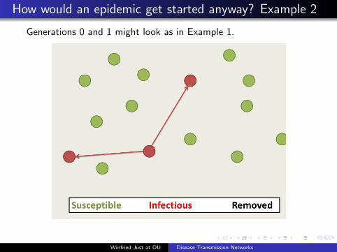
How would an epidemic get started anyway? Example 2
Generations 0 and 1 might look as in Example 1.
Ohio University – Since 1804 Department of MathematicsWinfried Just at OU Disease Transmission Networks

How would an epidemic get started anyway? Example 2
A new infection occurs.
Ohio University – Since 1804 Department of MathematicsWinfried Just at OU Disease Transmission Networks

How would an epidemic get started anyway? Example 2
An infectious host is removed.
Ohio University – Since 1804 Department of MathematicsWinfried Just at OU Disease Transmission Networks

How would an epidemic get started anyway? Example 2
A new infection occurs.
Ohio University – Since 1804 Department of MathematicsWinfried Just at OU Disease Transmission Networks

How would an epidemic get started anyway? Example 2
A new infection occurs.
Ohio University – Since 1804 Department of MathematicsWinfried Just at OU Disease Transmission Networks

How would an epidemic get started anyway? Example 2
A new infection occurs.
Ohio University – Since 1804 Department of MathematicsWinfried Just at OU Disease Transmission Networks

How would an epidemic get started anyway? Example 2
An infectious host is removed.
Ohio University – Since 1804 Department of MathematicsWinfried Just at OU Disease Transmission Networks

How would an epidemic get started anyway? Example 2
A new infection occurs.
Ohio University – Since 1804 Department of MathematicsWinfried Just at OU Disease Transmission Networks

How would an epidemic get started anyway? Example 2
A new infection occurs.
Ohio University – Since 1804 Department of MathematicsWinfried Just at OU Disease Transmission Networks

How would an epidemic get started anyway? Example 2
A new infection occurs.
Ohio University – Since 1804 Department of MathematicsWinfried Just at OU Disease Transmission Networks

How would an epidemic get started anyway? Example 2
An infectious host is removed.
Ohio University – Since 1804 Department of MathematicsWinfried Just at OU Disease Transmission Networks

How would an epidemic get started anyway? Example 2
A new infection occurs.
Ohio University – Since 1804 Department of MathematicsWinfried Just at OU Disease Transmission Networks

How would an epidemic get started anyway? Example 2
A new infection occurs.
Ohio University – Since 1804 Department of MathematicsWinfried Just at OU Disease Transmission Networks

How would an epidemic get started anyway? Example 2
An infectious host is removed.
Ohio University – Since 1804 Department of MathematicsWinfried Just at OU Disease Transmission Networks

How would an epidemic get started anyway? Example 2
An infectious host is removed.
Ohio University – Since 1804 Department of MathematicsWinfried Just at OU Disease Transmission Networks

Some generations of the infection in Example 2
The average number of secondary infections per infectious host ingenerations 0 to 2 in this example is 2+2+0+2+3+2+3+1
8 = 158 .
Ohio University – Since 1804 Department of Mathematics
Winfried Just at OU Disease Transmission Networks

Does Example 2 indicate the start of an epidemic?
Most likely. From generation 0 to generation 3 the number ofinfectious hosts has increased by a factor of 8, and one mightexpect similar increases in subsequent generations.Ohio University – Since 1804 Department of MathematicsWinfried Just at OU Disease Transmission Networks

What makes the difference?
Definition
The expected number of secondary infections that will be causedby a single infectious host that is introduced into a large andentirely susceptible population is denoted by R0 and called thebasic reproductive ratio or basic reproductive number.
If R0 � N and if we assume uniform mixing of the population,then practically contacts of infectious hosts during the first fewgenerations will be with susceptibles, and we might assume, aslong as k is sufficiently small, that R0 ≈ Rk , where Rk denotes themean number of secondary infections caused by a host in the k-thgeneration.
Based on this argument, our best guess at R0 would beR0 ≈ 5
6 < 1 in Example 1 and R0 ≈ 158 > 1 in Example 2.
Ohio University – Since 1804 Department of Mathematics
Winfried Just at OU Disease Transmission Networks

R0 makes the difference
Theorem
Assume uniform mixing and introduction of a single infectedindividual into an entirely susceptible population. Assume,moreover, that R0 does not depend on N.
If R0 < 1, then the expected number of individuals that eventuallybecome infected is bounded by a constant that depends only on R0
but not on N, and the disease is predicted to quickly die out.
If R0 > 1, then with probability > 0 an epidemic whose final size isat least a fraction F (1,N) > 0 that depends only on R0 will occur.
“Proof”: Under the assumption the expected number of infectedsin generation k satisfies E (gk) = R0R1 . . .Rk−1 ≤ Rk
0 , sinceRk ≤ R0. Thus E (limt→∞N − S(t)) ≤
∑∞k=0 Rk
0 = 11−R0
.
If R0 > 1, then E (gk) ≈ Rk0 for small k . More generally, Rk ≥ 1
until a significant fraction of susceptibles move to the I - orR-compartments; an epidemic will occur with positive probability.Ohio University – Since 1804 Department of MathematicsWinfried Just at OU Disease Transmission Networks

Which factors might determine R0 and, more generally, thedisease dynamics?
The pattern of mixing between susceptibles and infectives. Wewould like to know, for a given susceptible host and a giventime interval, the probability distribution of the number andintensity of contacts that this host will have with infectives.
The probability that a given contact between a susceptibleand infective individual at time T i
I + t results in a “successful”(from the point of view of the disease agent) transmission.
The distribution of times T iI − T i
E during which a host residesin E and T i
R − T iI during which a host resides in I .
This may be too much to ask (the biologists) for.
Can you think of a population of real hosts for which itwould be possible to collect all the relevant data?
Even if we could have all the data, the resulting model would likelybe intractable. We need to make simplifying assumptions.Ohio University – Since 1804 Department of Mathematics
Winfried Just at OU Disease Transmission Networks

We have seen extreme simplifications
The compartment-based ODE models that we saw earlier distill allthese features into two parameters α and β. This may be tooextreme. In particular:
ODE models ignore the stochastic nature of diseasetransmission.
Compartment models ignore heterogeneities betweenindividual hosts.
Compartment models are based on the often unrealisticassumption of uniform mixing between individual hosts.
Let us now try to develop a modeling framework that is capable ofincorporating as many potentially relevant details as possible.
Ohio University – Since 1804 Department of Mathematics
Winfried Just at OU Disease Transmission Networks

Stochastic process models: The basics
Examples 1 and 2 suggest that stuff happens at random times T iI
of infection and T iR of removal of host number i .
One can conceptualize disease dynamics as a stochastic processthat moves hosts around between the compartments.
Let us assume a fixed population that consists of hosts that arerepresented by variables xi (t), where i ∈ {1, . . . , n}.
At any given time, a r.v. xi (t) can take values xi (t) ∈ {S , I ,R},depending on the relation of t to T i
I and T iR .
The state of the population at time t is the vector~x(t) = (x1(t), . . . , xN(t)).
Ohio University – Since 1804 Department of Mathematics
Winfried Just at OU Disease Transmission Networks

What have we swept under the rug so far?
We ignore demographics, that is births, deaths from unrelatedcauses, immigration and emigration.
We assumed T iI = T i
E , that is, the time of exposure coincideswith the onset of infectiousness.
Successful transmission is a discrete event that either does ordoes not happen during a given contact between an infectiveand susceptible host. This ignores the possibility of multiplebelow-threshold exposures adding up to an infection.
How distorting are these simplifying assumptions likely to be?
How could we incorporate the ignored details into our model?
Ohio University – Since 1804 Department of Mathematics
Winfried Just at OU Disease Transmission Networks

Independence of transition times
A state can change only by a variable xi changing its state from Sto I (at time T i
I ) or from I to R (at time T iR).
We will assume that for any given state ~x(t) the relevantvariables T i
I and T iR are all independent.
How realistic is this assumption?
Ohio University – Since 1804 Department of Mathematics
Winfried Just at OU Disease Transmission Networks

The Markov Property
We want our stochastic process model to be reasonably tractable;the Markov Property might help. In other words, given a state ~x ,we want the conditional distribution of future states ~x(t + ∆t)given that ~x(t) = ~x to depend only on ~x and ∆t. One advantageof the Markov Property is that it allows in some cases forapproximations of the model by autonomous ODEs.
The Markov Property implies that for a given state ~x each of therelevant variables T i
I = T iI (~x) and T i
R = T iR(~x) is memoryless.
Thus T iI will be exponentially distributed with parameter βi (~x) and
T iR will be exponentially distributed with parameter αi (~x).
Ohio University – Since 1804 Department of Mathematics
Winfried Just at OU Disease Transmission Networks

Surprise: We have built a model!
Now assume you can determine values for the parameters αi (~x)and βi (~x) for all possible states ~x of the population. Then theabove assumptions specify a stochastic model. Let’s show how tosimulate the process on the computer.
Choose an initial state ~x := ~x(0).For all i with xi = I , randomly and independently choosetimes T i
R at which host i will move out of the I -compartmentaccording to an exponential distribution with parameter αi (~x).For all i with xi = S , randomly and independently choosetimes T i
I at which host i would move into the I -compartmentif the state were to remain unchanged, according to anexponential distribution with parameter βi (~x).Determine the smallest time tnext at which the next “event”(movement of a host to a different compartment) happens.Set ~x := ~x(tnext) accordingly.Repeat until stopping criterion.
Ohio University – Since 1804 Department of Mathematics
Winfried Just at OU Disease Transmission Networks

Advantages of the supermodel
We can think of the construction we have just presented as asupermodel. It has a lot of attractive features:
It accounts for the stochastic nature of disease transmission.
It can be easily explored by simulations for moderatelylarge N.
It allows for heterogeneities between individual hosts (think ofαi (~x) as reflecting individual strength of the immune system).
It allows for exploring a variety of mixing patterns betweenindividual hosts (since βi (~x) in general may depend on ~x , thatis, on which other hosts are infectious at a given time).
Can you think of a scenario where we would want αi (~x) toactually depend on ~x?
Ohio University – Since 1804 Department of Mathematics
Winfried Just at OU Disease Transmission Networks

A drawback of the Markov Property
The Markov Property may impose some plainly unrealistic featuresthough.
For example, the assumption that T iR − T i
I is a memoryless r.v. isblatantly wrong for most diseases. Recovery times show usually adistribution that peaks at some modal value. For example, you aremuch more likely to recover during day 7 of a bout of the flu thanduring day 2, while an exponential distribution would predict theopposite.
How can we modify the model so that the distribution ofrecovery times becomes more realistic without sacrificing theMarkov Property of the process?
Ohio University – Since 1804 Department of Mathematics
Winfried Just at OU Disease Transmission Networks

Beware of supermodels!
Supermodels are pleasant to contemplate, but notoriously difficultto work with.
Here are some problems ours suffers from:
There are just too many parameters. For an SIR-model wewould need 2N3N parameters βi (~x) and αi (~x).
Even for relatively small N it is plainly impossible to estimatethat many parameters from any kind of data.
The dimension N of the model is too large to study itanalytically.
Can we reduce the number of parameters that need to beestimated from the data?
Ohio University – Since 1804 Department of Mathematics
Winfried Just at OU Disease Transmission Networks

Let’s make some tough choices
Let us ignore heterogeneities in individual immune responseand set αi (~x) to a fixed α for all i and ~x .There is only one type of contact, and contacts last an instantrather than having a duration. The probability of a“successful” transmission of the disease during a givencontact between an infectious and a susceptible host is a fixedparameter p.The time τi ,j that host number i has to wait for the nextcontact with host number j after time t is a memoryless r.v.and thus has an exponential distribution with someparameter λi ,j that does not depend on ~x .
This still allows us to explore a variety of mixing patterns andreduces the number of parameters from a stratospheric 2N3N to astill lofty but more reasonable
(N2
)+ 2.
What are some potential problems with these assumptionsand how could we address them?Ohio University – Since 1804 Department of Mathematics
Winfried Just at OU Disease Transmission Networks

The new parameters specify a model
αi (~x) = α for a fixed α for all i and ~x .The probability of a “successful” transmission of the diseaseduring a given contact between an infectious and a susceptiblehost is a fixed parameter p.The time τi ,j that host number i has to wait for the nextcontact with host number j has an exponential distributionwith some parameter λi ,j .
We need to convince ourselves that the new parameters p and λi ,jsuffice to specify βi (~x) for all i and ~x .
For sufficiently small ∆t the probability that a successfultransmission from infectious host number j to susceptible hostnumber i occurs in the interval [0,∆t] can be approximated asP(τi ,j ≤ ∆t)p ≈ pλi ,j∆t,and the probability that susceptible host number i will becomeinfected during this time interval can be approximated asP(T i
I (~x) < ∆t) ≈∑{j : x(j)=I} pλi ,j∆t = βi (~x)∆t.
Ohio University – Since 1804 Department of MathematicsWinfried Just at OU Disease Transmission Networks

The uniform mixing assumption
The uniform mixing assumption translates into
λi ,j = λ for some fixed constant λ,
or, equivalently, into
βi (~x) = pλ#{j : x(j) = I} = β#{j : x(j) = I}for the fixed constant β = pλ.
One can also interpret β#{j : x(j) = I} as the rate at whichsusceptible host number i acquires an infection; it is called theforce of infection.
For large N, this allows us to approximate our stochastic processmodels by the ODE models that we encountered earlier.
Ohio University – Since 1804 Department of Mathematics
Winfried Just at OU Disease Transmission Networks

Basic ODE versions of the SI -, SIR- and SIS-models
SI -model:
dSdt = −βSIdIdt = βSI
SIS-model:
dSdt = −βIS + αIdIdt = βIS − αI
SIR-model:
dSdt = −βISdIdt = βIS − αIdRdt = αI
Ohio University – Since 1804 Department of Mathematics
Winfried Just at OU Disease Transmission Networks

The uniform mixing assumption
The uniform mixing assumption translates into
λi ,j = λ for some fixed constant λ,
or, equivalently, into
βi (~x) = pλ#{j : x(j) = I} = β#{j : x(j) = I}for the fixed constant β = pλ.
We get a reduction to only two parameters.
But when would the the uniform mixing assumption berealistic?
Mixing may be nearly uniform if hosts move around a lot relativeto the size of the habitat, encounter each other rarely, and there isno social structure.
Ohio University – Since 1804 Department of Mathematics
Winfried Just at OU Disease Transmission Networks

How to model more realistic mixing patterns?
In populations with a well-defined social or territorial structurethough, some pairs of individuals will have contact relativelyfrequently (think of co-workers or neighbors in humanpopulations), while other pairs of individuals will almost certainlynever encounter each other (think of your likelihood to ever meetthe Supreme Leader of North Korea).
We can approximate the latter situation by assuming the existenceof a contact network which determines whether it is even possiblethat the disease can be transmitted between two given hosts.
The nature of the required contact, and thus the relevant contactnetwork, may depend on the particular disease. Think of the flu vs.a computer virus vs. a sexually transmitted disease.
Ohio University – Since 1804 Department of Mathematics
Winfried Just at OU Disease Transmission Networks

Mathematical structures for modeling contact networks:graphs
A graph is an ordered pair G = (V ,E ), where V denotes the set ofvertices, or nodes, and the set E of edges of G is a subset of theset of unordered pairs of nodes.
A contact network can be modeled as a graph whose vertices arethe individual hosts in the population, and an edge between twohosts signifies an above-threshold probability of a relevant contactbetween these two hosts.
One can then make the simplifying assumption that diseasetransmission can occur only between two hosts that are representedby adjacent nodes, that is, endpoints of a common edge, and studythe possible or likely dynamics of the disease on the network.
Ohio University – Since 1804 Department of Mathematics
Winfried Just at OU Disease Transmission Networks

An example of a contact network
Ohio University – Since 1804 Department of Mathematics
Winfried Just at OU Disease Transmission Networks

Could Example 1 occur on this contact network?
Ohio University – Since 1804 Department of Mathematics
Winfried Just at OU Disease Transmission Networks

Could Example 1 occur on this contact network?
Ohio University – Since 1804 Department of Mathematics
Winfried Just at OU Disease Transmission Networks

Could Example 1 occur on this contact network?
Ohio University – Since 1804 Department of Mathematics
Winfried Just at OU Disease Transmission Networks

Could Example 1 occur on this contact network?
Ohio University – Since 1804 Department of Mathematics
Winfried Just at OU Disease Transmission Networks

Could Example 1 occur on this contact network?
Ohio University – Since 1804 Department of Mathematics
Winfried Just at OU Disease Transmission Networks

Could Example 1 occur on this contact network?
Ohio University – Since 1804 Department of Mathematics
Winfried Just at OU Disease Transmission Networks

Could Example 1 occur on this contact network?
Ohio University – Since 1804 Department of Mathematics
Winfried Just at OU Disease Transmission Networks

Could Example 2 occur on this contact network?
Ohio University – Since 1804 Department of Mathematics
Winfried Just at OU Disease Transmission Networks

Could Example 2 occur on this contact network?
Ohio University – Since 1804 Department of Mathematics
Winfried Just at OU Disease Transmission Networks

Could Example 2 occur on this contact network?
Ohio University – Since 1804 Department of Mathematics
Winfried Just at OU Disease Transmission Networks

Could Example 2 occur on this contact network?
Ohio University – Since 1804 Department of Mathematics
Winfried Just at OU Disease Transmission Networks

Example 2 could not occur on this contact network
Ohio University – Since 1804 Department of Mathematics
Winfried Just at OU Disease Transmission Networks

One last simplifying assumption
Let us assume that for some fixed constant λ we have λi ,j = λwhenever {i , j} is an edge in the contact network, and λ = 0otherwise.
This assumption strictly speaking does not reduce the number ofparameters, but it allows us to define stochastic process modelspurely in terms two real parameters α and β and the contactnetwork, which is a discrete structure.
Ohio University – Since 1804 Department of Mathematics
Winfried Just at OU Disease Transmission Networks

Stochastic process models for disease transmission onnetworks
Ingredients:
Specification of the type of model (SI , SIR, or SIS).
A graph G with N vertices that represents the contactnetwork.
A parameter α that represents the removal rate.
A parameter β = pλ that specifies the rate at which a givensusceptible host acquires infections from a given adjacentinfectious host.
The process will then be modeled as described above, with
βi (~x(t)) = β#{j : xj(t) = I & {i , j} ∈ E}.
Ohio University – Since 1804 Department of Mathematics
Winfried Just at OU Disease Transmission Networks

But how to model the network?
A major problem is that we usually have only very limitedknowledge of the actual contact network. There are basically twoways of building mathematically meaningful models of theunderlying networks.
In some cases the network may have a very special structurethat can be determined from data.Alternatively, we can assume that the network is randomlydrawn from a probability distribution with certain parameters.The values of these parameters should be chosen in such away that they favor networks with properties that conform towhatever data we have about the actual network.Popular choices for the second alternative are Erdos-Renyirandom graphs or scale-free networks that can be randomlygenerated according to the preferential attachment model. Inthe hands-on part we will explore several types of randomgraphs.
Ohio University – Since 1804 Department of Mathematics
Winfried Just at OU Disease Transmission Networks

What is to be gained from network models of diseasetransmission?
While the kind of network models we defined here are morerealistic than compartment models, they still are based on a lot ofsimplifying assumptions. But they can give us important insights:
They can make predictions about the probability of anepidemic that are not available from ODE models.They may point to features of the contact network thatsignificantly influence the outcome of an epidemic. This givessome guidance about what kind of data we need to collect inorder to be able to make reasonably accurate predictions.They may allow us to discern cases when acompartment-based model is inadequate or, alternatively,guide our choice of the parameters for compartment-basedmodels.They can inform the design of effective control measures whenthe uniform mixing assumption is inadequate.
Ohio University – Since 1804 Department of MathematicsWinfried Just at OU Disease Transmission Networks

Exhibit A: the uniform mixing assumption revisited
The uniform mixing assumption corresponds to the case where Gis the complete graph that contains all possible edges.
Assume an SIR model. To estimate R0, consider a state ~x(0) withexactly one infectious host, number j , and all other hosts beingsusceptible.
Then the expected number of transmissions over a small timeinterval of length ∆t from host j to a given host i is ≈ β∆t, thusthe expected overall number of secondary infections caused byhost j over this interval is ≈ β(N − 1)∆t.
This formula applies as long as the interval is contained in (0,T jR).
Expected values add up, so if we partition (0,T jR) into small
subintervals of length ∆t each, we can deduce that the expectedoverall number of secondary infections caused by host j satisfies
R0 ≈ β(N − 1)∆tE(T j
R)∆t = β(N−1)
α .Ohio University – Since 1804 Department of Mathematics
Winfried Just at OU Disease Transmission Networks

When is this approximation valid?
I haven’t been very clear about all the assumptions needed for thisapproximation to be a good one.
We will explore in the hands-on session what extraassumptions are needed here and why.
Ohio University – Since 1804 Department of Mathematics
Winfried Just at OU Disease Transmission Networks

Exhibit A: compare this with the ODE model
dSdt = −βISdIdt = βIS − αI = I (βS − α)dRdt = αI
If one infectious individual is introduced into an otherwisesusceptible population, then S = N − 1. For β < α
N−1 , the modelpredicts a decrease in I ; for β > α
N−1 , an initially exponentialincrease of this variable. Reasoning backwards from the theoremabout R0, we see that R0 = β(N−1)
α , the same as for the stochasticprocess model. This assumes population size expressed by thenumber of individuals; for units of, say, thousands of individuals weget R0 ≈ βN
α . R0 it is often reported in these forms.
But the ODE model predicts that for R0 > 1 an epidemic willalways occur for this initial condition, while the stochastic natureof transmission implies that this happens only with a positiveprobability < 1.
The network model allows us to determine this probability.Ohio University – Since 1804 Department of MathematicsWinfried Just at OU Disease Transmission Networks

Exhibit B: When is R0 a good predictor?
The inequality R0 > 1 is supposed to predict a positive probabilityof an epidemic, with initially exponential increase in the number ofinfected hosts.
This theorem was based on the uniform mixing assumption.
When does this prediction fail?If it fails, what may be a better predictor?
We will explore this issue with random networks and the followingtwo special networks.
Ohio University – Since 1804 Department of Mathematics
Winfried Just at OU Disease Transmission Networks

Special case 1: L×M rectangular grids
Think of a banana plantation where the disease agent can moveonly by a distance of at most 1.Ohio University – Since 1804 Department of Mathematics
Winfried Just at OU Disease Transmission Networks

Special case 2: Rectangular grids with diagonal edges
Think of a banana plantation where the disease agent can moveonly by a distance of at most 1.5.Ohio University – Since 1804 Department of Mathematics
Winfried Just at OU Disease Transmission Networks

Exhibit C: Trees
A tree is a connected graph with exactly one path between eachpair of nodes. The nodes with degree 1 are called leaves.
Think of a river system.Ohio University – Since 1804 Department of MathematicsWinfried Just at OU Disease Transmission Networks

Exhibit C: Protecting rivers
Think of a river system. An invasive species, for example,freshwater mussels, may spread along the river. This seemsdifferent from disease transmission, but think again:
The mussels would be the disease agents here.The hosts would be branching points of the river system.An SI -type network model seems appropriate.The spread of mussels along river segments could be blockedby physical barriers. This is mathematically equivalent tobehavior modification (think “unfriending”).Alternatively, branching points could be protected byintroducing predators in large enclosures. This ismathematically equivalent to immunization.Either control measure is expensive.
Given a limited budget, where should we place the predatorsor barriers?We will explore various strategies with the help of random trees.Ohio University – Since 1804 Department of Mathematics
Winfried Just at OU Disease Transmission Networks